Optimization of snow cover fraction parameterization in the Community Land Model: implementation and preliminary validation over the Tibetan Plateau

Snow cover over the Tibetan Plateau (TP) is not only a key land forcing for the regional and global climate but also an important water resource for surround regions. However, state-of-the-art climate models still exhibit substantial biases in simulating winter snow cover over the TP, which constitutes one of the major sources of uncertainty in climate prediction. Using satellite-based snow cover datasets, this study reveals that the Community Land Model version 5 (CLM5) systematically overestimates the winter snow cover fraction (SCF) over the TP. This bias mainly arises because the original SCF parameterization scheme neglects the spatially varying probability distribution of snowfall accumulation and underestimates snow depletion over barren land during the melting period. By accounting for the effects of non-growing-season low vegetation (i.e., withered grass stems) and topographic relief, we parameterize the snow accumulation probability factor (k_accum) instead of prescribing it as a constant. In addition, a revised factor is introduced to modify the snow depletion curve shape parameter (N_melt), thereby optimizing the SCF parameterization scheme. Preliminary validation indicates that the optimized scheme substantially reduces positive winter SCF biases over the entire TP by 63 %, and improves surface albedo simulations, thereby alleviating cold surface temperature biases by approximately 1–2 °C in snow-affected regions.

1 Introduction

Snow cover is a key parameter on the land surface due to its high albedo and hydrological effects of snowmelt, greatly affecting the surface energy balance and water cycle, plays an important role in climate system (e.g., Wang et al., 2017; Henderson et al., 2018; Yang et al., 2023). Accurate parameterization of snow cover is critical for the performance of numerical models in weather and climate simulations and predictions, particularly in high-latitude and high-altitude regions (Toure et al., 2016). Previous studies have indicated that biases in simulated snow cover over the Tibetan Plateau (TP) are among the primary causes of errors in local near-surface air temperature simulations and contribute substantially to uncertainties in climate simulations over East Asia (Orsolini et al., 2019; Zhou et al., 2023). Therefore, optimizing snow cover parameterizations in land surface models (LSMs) remains essential for improving the capability of numerical models to simulate and predict weather and climate.

Over the past decades, snow cover parameterizations have been substantially developed (e.g., Niu and Yang, 2007; Swenson and Lawrence, 2012; Vionnet et al., 2012; van Kampenhout et al., 2017; Lawrence et al., 2019). In addition, considerable efforts have been made to improve simulations of snow cover and associated surface energy processes over the TP by accounting for blowing snow, complex topography, and snow albedo variations. For example, Xie et al. (2019) coupled a blowing snow model (PIEKTUK) with the Community Land Model version 4.5 (CLM4.5) and improved simulations of snow dynamics over most regions of the TP. Based on station observations and simulations with the SNICAR radiative transfer model, Wang et al. (2020) developed a fresh snow albedo scheme in the Noah-MP land surface model, which effectively reduced excessive snow depth biases over the TP. Liu and Ma (2024) further showed that an improved albedo scheme – by optimizing snow age parameters and explicitly accounting for snow depth in the Noah land surface model – enhanced snow cover simulations in the Weather Research and Forecasting (WRF) model during snow events over the TP. The Community Land Model version 5 (CLM5), the latest LSM developed by the US National Center for Atmospheric Research (NCAR), incorporates substantial improvements in snow cover parameterization compared with its predecessor, CLM4 (Lawrence et al., 2019). These developments include separate calculations of snow cover fraction (SCF) for accumulation and depletion stages, representations of topographic effects on snowmelt, and the influence of wind and air temperature on fresh snow density (van Kampenhout et al., 2017). Nevertheless, pronounced biases in snow cover simulations persist over high-latitude regions and the TP in both CLM4 (Toure et al., 2016) and CLM5 (Ma and Wang, 2022). Moreover, cold surface temperature biases over the TP remain evident in most CMIP6 models (Cui et al., 2021). Thus, further comprehensive improvements to snow cover parameterizations are still required, even in the latest and relatively well-developed LSMs.

In LSMs, one of the largest sources of uncertainty in simulating snow cover and the surface energy budget arises from snow cover fraction (SCF) parameterizations (Niu and Yang, 2007; Swenson and Lawrence, 2012). Traditionally, SCF parameterizations are formulated based on the relationship between SCF and snow depth, with empirical parameters introduced to represent subgrid-scale variability and surface heterogeneity (Liston, 2004). Over the TP, the land surface exhibits pronounced spatial heterogeneity, characterized by large topographic relief and diverse low-stature vegetation. Previous studies have investigated the influence of topography on SCF (e.g., Douville et al., 1995; Lopez-Moreno and Stähli, 2008). Recently, Miao et al. (2022) demonstrated that SCF simulation biases in the Simplified Simple Biosphere Model version 3 (SSiB3) can be reduced by accounting for topographic effects, suggesting that more complex terrain tends to produce a smaller snow-covered extent for a given amount of snow. In contrast, Zhang et al. (2022) showed that incorporating a three-dimensional subgrid terrain radiative effect scheme effectively diminishes the overestimation of surface solar radiation and alleviates warm land surface temperature biases, highlighting the shading and cooling effects of complex terrain. This implies that increased topographic complexity may also retard snowmelt. Therefore, the effects of topography on snow cover appear to be twofold, yet this dual role is not fully represented in current LSMs. In addition, snow cover over most regions of the TP is generally shallow, such that low vegetation – particularly withered grass stems (WGS) and branches over the southern and eastern TP – is not completely buried by snow. Recent studies have suggested that WGS can enhance snowmelt over the TP by altering surface energy exchange processes (Yang et al., 2023; Qi et al., 2024), an effect that is largely neglected in existing LSMs. Consequently, how to explicitly incorporate the influences of pronounced topographic relief and WGS into SCF parameterizations remains a challenging but critical issue.

This study addresses two main objectives. First, it investigates the characteristics of winter snow cover simulation biases over the TP in CLM5 and explores their potential causes from the perspective of deficiencies in the SCF parameterization. Second, it seeks to optimize the SCF parameterization by comprehensively accounting for the effects of topography and WGS. The remainder of this paper is organized as follows. Section 2 describes the data and methodology. Section 3 presents the optimization of the SCF parameterization and the experimental design used to evaluate both the original and optimized schemes. Section 4 reports the model results, including an analysis of winter snow cover biases simulated by CLM5, validation of the optimized scheme, and its impacts on the surface energy budget. Section 5 discusses uncertainties related to snowfall in LSMs, remaining challenges and potential applicability of the optimized scheme. Finally, conclusions are presented in Sect. 6.

2 Data and methods

2.1 Meteorological forcing and validation dataset

To conduct the offline simulation of CLM5 over the TP, the 3-hourly China meteorological forcing dataset v1.6 (CMFD 1.6; https://data.tpdc.ac.cn/zh-hans/data/8028b944-daaa-4511-8769-965612652c49/, last access: 29 June 2026) (Yang et al., 2010; He et al., 2020) with a horizontal resolution of 0.1°×0.1° for the period 1979–2018 was obtained, CMFD 1.6 includes the surface air temperature, surface pressure, specific humidity, wind speed, precipitation, downward shortwave and longwave radiation.

To validate the CLM5 simulations of snow cover over the TP, a daily cloudless Moderate Resolution Imaging Spectroradiometer (MODIS) snow area ratio dataset (2000–2015) with the 500 m spatial resolution (https://data.tpdc.ac.cn/en/data/94a8858b-3ace-488d-9233-75c021a964f0/, last access: 29 June 2026) was obtained, this dataset is obtained by using a cloud removal algorithm based on cubic spline interpolation (Tang et al., 2013). A daily, 0.05° snow depth dataset for TP (2000–2021) (https://data.tpdc.ac.cn/en/data/0515ce19-5a69-4f86-822b-330aa11e2a28/, last access: 29 June 2026) was also used, which is obtained based on the sub-pixel spatio-temporal downscaling algorithm and the fusion of snow cover probability dataset and Long-term snow depth dataset in China (Yan et al., 2022).

To analyze the effects of the optimized SCF parameterization scheme on surface energy budget, the Global Land Surface Satellites (GLASS) albedo products (Liang et al., 2021; https://glass.hku.hk/archive/Albedo/MIX/0.05D/, last accesss: 29 June 2026) with a 0.05°×0.05° spatial resolution and 8 d temporal resolution from 2002 to 2011 was used, and the monthly data was averaged from it. The MODIS monthly land surface temperature product with a 0.05°×0.05° spatial resolution from 2002 to 2011 was also used (https://ladsweb.modaps.eosdis.nasa.gov/missions-and-measurements/products/MOD11C3, last access: 29 June 2026).

The 0.05°×0.05° and 500 m dataset was averaged to the 0.1°×0.1° for the convenient comparison with CLM5 simulations.

2.2 Standard deviation of topography and stem area index (SAI) dataset

In this study, the grid cell standard deviation of topography for the SCF parameterization was calculated based on the elevation data obtained from the USGS HYDRO1K 1 km dataset (https://doi.org/10.5066/F77P8WN0, USGS, 2026). The SAI data which is used as the proxy of WGS area or coverage is derived from a MODIS consistent land surface parameters dataset (Lawrence and Chase, 2007; https://svn-ccsm-inputdata.cgd.ucar.edu/trunk/inputdata/lnd/clm2/mappingdata/grids/, last access: 29 June 2026).

2.3 Validation metrics

The mean bias error (MBE), root mean square error (RMSE) were used to quantify the errors of model simulations, which are calculated as follows:

$$\begin{array}{}\text{(1)}& {\displaystyle }& {\displaystyle }\mathrm{MBE}={\displaystyle \frac{\mathrm{1}}{n}}\sum _{i=\mathrm{1}}^n\left(x_{\mathrm{s},i}-x_{\mathrm{o},i}\right)\text{(2)}& {\displaystyle }& {\displaystyle }\mathrm{RMSE}=\sqrt{{\displaystyle \frac{\mathrm{1}}{n}}\sum _{i=\mathrm{1}}^n{\left(x_{\mathrm{s},i}-x_{\mathrm{o},i}\right)}^{\mathrm{2}}}\end{array}$$

where x_s,i and x_o,i represent the simulated value and observed value, respectively, n represents the sequence length.

The spatial correlation coefficient (R) was also adopted to quantify the capability of model in reproducing the spatial pattern of snow cover and the related variables, which is calculated as follows:

$$\begin{array}{}\text{(3)}& R={\displaystyle \frac{\sum _{i=\mathrm{1}}^n\left(x_{\mathrm{s},i}-\stackrel{\mathrm{‾}}{x_{\mathrm{s},i}}\right)\cdot \left(x_{\mathrm{o},i}-\stackrel{\mathrm{‾}}{x_{\mathrm{o},i}}\right)}{\sqrt{\sum _{i=\mathrm{1}}^n{\left(x_{\mathrm{s},i}-\stackrel{\mathrm{‾}}{x_{\mathrm{s},i}}\right)}^{\mathrm{2}}}\cdot \sqrt{\sum _{i=\mathrm{1}}^n{\left(x_{\mathrm{o},i}-\stackrel{\mathrm{‾}}{x_{\mathrm{o},i}}\right)}^{\mathrm{2}}}}}\end{array}$$

where $\stackrel{\mathrm{‾}}{x_{\mathrm{s},i}}$ and $\stackrel{\mathrm{‾}}{x_{\mathrm{o},i}}$ represent the mean of simulated value and observed value, respectively.

2.4 Selection of daily snowfall events and snowmelt events

In this study, the SCF parameterization is optimized separately for snowfall and snowmelt processes at a daily timescale. Accordingly, daily snowfall and snowmelt events need be identified.

Because direct observations of snowfall are unavailable, daily positive changes in the observed snow depth which is obtained from 0.05° downscaling product over the TP (the detail seen in Sect. 2.1) are used as a proxy to identify the occurrence and approximate magnitude of snowfall. For each year during the period 2003–2012 (10 years), the 10 d with the largest increases in snow depth are selected, yielding a total of 100 snowfall events. These snowfall amounts are then sorted from the smallest to the largest, and the resulting sequence is treated as a continuous snow accumulation process.

Similarly, daily negative changes in the observed snow depth are adopted as a proxy for snowmelt. For each year from 2003–2012, the 10 d with the largest decreases in snow depth are selected, resulting in a total of 100 snowmelt events. These snowmelt amounts are subsequently sorted from the largest to the smallest, and the ordered sequence is regarded as a continuous snow depletion process.

It is acknowledged that daily changes in snow depth do not strictly represent actual snowfall and snowmelt amounts. However, the associated uncertainties are considered acceptable, as these quantities are not directly used in the SCF calculations.

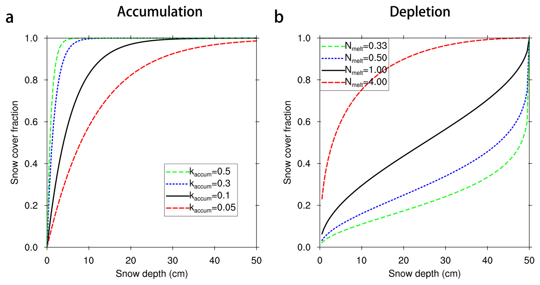
Figure 1 Relationship between snow cover fraction (SCF) and snow depth. (a) Accumulation curves of SCF with increase of snow depth (d_snow; cm) during snowfall under different values of probability distribution factor (k_accum) according to Eq. (4), here, amount of new snow (q_snow⋅Δt; mm) is calculated by multiplying Δd_snow by snow density (ρ_snow; kg m⁻³). (b) Depletion curves of SCF under different values of N_melt according to Eq. (5).

3 SCF parameterization optimization and experimental design

3.1 Current SCF parameterization in CLM5

This study adopted CLM5 which was well developed in descriptions of surface energy fluxes and hydrology processes (Lawrence et al., 2019). In CLM5, the parameterization of SCF (f_snow) is based on the method of Swenson and Lawrence (2012). Because the processes governing snowfall and snowmelt differ, changes in f_snow (%) are calculated separately for accumulation and depletion. When snowfall occurs, f_snow is updated as

$$\begin{array}{}\text{(4)}& f_{\mathrm{snow}}^{n+\mathrm{1}}=\mathrm{1}-\left(\left(\mathrm{1}-\tanh \left(k_{\mathrm{accum}}{q}_{\mathrm{snow}}\mathrm{\Delta }t\right)\right)\left(\mathrm{1}-f_{\mathrm{snow}}^n\right)\right)\end{array}$$

where tanh (k_accumq_snowΔt) is the probability distribution of snow cover during snowfall, k_accum is the probability distribution factor (unitless), whose default value is 0.1, q_snowΔt is the amount of new snow (mm). According to Eq. (4), accumulation curves of SCF with increase of snow depth during snowfall under different values of k_accum are shown in Fig. 1a, which describes the SCF increases rapidly when the snow depth is shallow (i.e., at the onset of snowfall) and subsequently changes more gradually.

When snow melts, f_snow is calculated from the depletion curve:

$$\begin{array}{}\text{(5)}& f_{\mathrm{snow}}=\mathrm{1}-{\left({\displaystyle \frac{{\cos }^{-\mathrm{1}}\left(\mathrm{2}{R}_{\mathrm{snow}}-\mathrm{1}\right)}{\mathit{\pi }}}\right)}^{N_{\mathrm{melt}}}\end{array}$$

where R_snow (unitless) is the ratio of snow water equivalent (W_snow; mm) to the maximum accumulated snow water equivalent (W_max; mm). W_snow is directly calculated in CLM5, and W_max is determined by integrating snowfall amounts into snow water equivalent during snowfall events and is subsequently derived from the snow depletion curve. In other words, W_max is a diagnostic variable introduced to ensure consistency between the updated SCF and the total snow water equivalent. N_melt is the depletion curve shape parameter (unitless), which depends on the topographic variability within the grid cell:

$$\begin{array}{}\text{(6)}& N_{\mathrm{melt}}={\displaystyle \frac{\mathrm{200}}{\min \left(\mathrm{10},{\mathit{\sigma }}_{\mathrm{topo}}\right)}}\end{array}$$

where σ_topo (m) is the standard deviation of topography within a grid cell. Figure 1b shows the SCF depletion curves calculated using Eq. (5), the depletion patterns vary substantially with different values of N_melt, indicating a strong influence of N_melt on the shape of the depletion curves.

3.2 Optimizing SCF parameterization during snowfall by parameterizing the probability distribution coefficient (k_accum)

According to Eq. (4), the value of k_accum determines the accumulation rate of the snow cover fraction (SCF): smaller k_accum values lead to slower accumulation rates and smaller SCF, even under the same snowfall amount (Fig. 1a). However, in the current scheme, k_accum is treated as a constant with a default value of 0.1. In reality, different underlying surface types (e.g. barren, grass, shrub) are expected to influence the probability distribution of snow during snowfall (Sturm et al., 2001). In other words, k_accum should vary spatially rather than remain constant. Therefore, the current scheme likely fails to adequately represent the effects of underlying surface heterogeneity on snow accumulation.

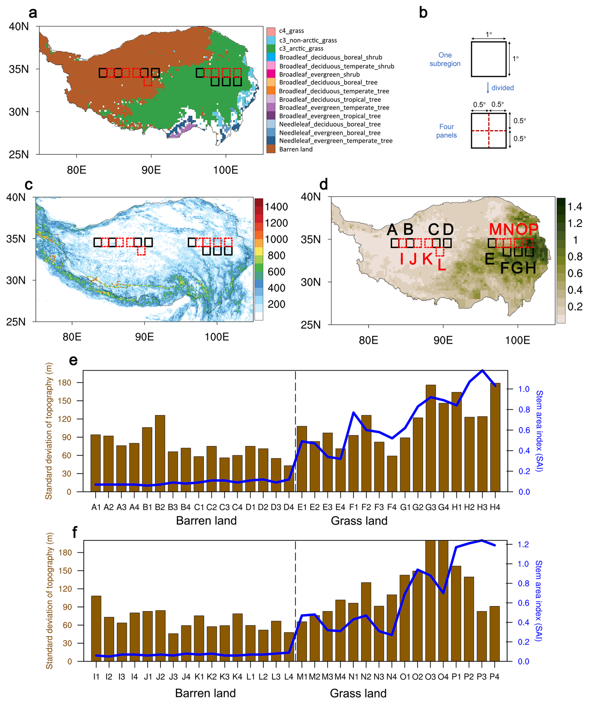
Figure 2 Subregions selected for analysis. (a) Underlying surface type over the TP. (b) Schematic diagram of dividing. Spatial distribution of (c) standard deviation of topography (σ_topo; m) within a grid cell, (d) stem area index (SAI; unitless) in October over the TP. Eight black rectangles (group 1) and eight red rectangles (group 2) represent subregions selected for analysis, one subregion (1°×1°) divided into four panels (0.5°×0.5°) as shown in (b) schematic diagram; thus there are thirty-two panels for both group 1 and group 2. Evolution of σ_topo and SAI across 32 panels for (e) group 1 and (f) group 2.

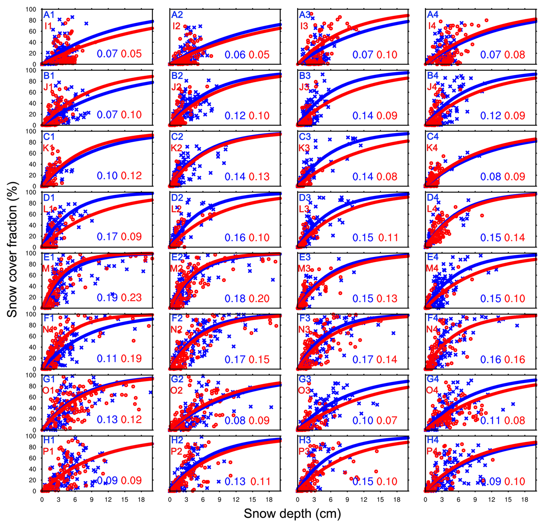
Figure 3 Observed relationship between snow cover fraction (SCF; %) and snow depth (cm) in 0.1×0.1 grid cells of 32 panels of group 1 (blue crosses) and group 2 (red circles) during snowfall over the TP. The fitted lines are computed from Eq. (4) with the optimal values of k_accum (blue and red font numbers are from group 1 and group 2, respectively) which were estimated when RMSE between observed SCF and the fitted value are smallest.

To estimate optimal values of k_accum under different land cover types, topographic relief, and vegetation conditions (Fig. 2), eight subregions were selected across the western, central, and eastern TP. As shown in Fig. 2a, barren land and alpine grassland dominate most areas of the TP. Accordingly, eight 1°×1° subregions (A–D, I–L) located in barren land and another eight subregions of the same size (E–H, M–P) located in alpine grassland were selected. To reduce uncertainties in the analysis, the selected subregions were divided into two independent groups. Group 1 consists of subregions A–D and E–H (black rectangles in Fig. 2d), whereas group 2 consists of subregions I–L and M–P (red rectangles in Fig. 2d). Each 1°×1° subregion was further divided into four 0.5°×0.5° panels (Fig. 2b), yielding a total of 32 panels in each group. These panels exhibit distinct differences in topographic relief (σ_topo) and SAI (Fig. 2c–e). Together, these variations effectively represent the heterogeneity of underlying surface conditions across the TP. It should be noted that, current SCF scheme in CLM5 mainly considered effects of large topographic relief (σ_topo>200 m) on snowmelt (Swenson and Lawrence, 2012), while neglecting the fact that smaller topographic relief can also induce substantial SCF simulation biases (Miao et al., 2022). Therefore, σ_topo values in the selected panels are generally smaller than 200 m, and this study focused on effects of topography at this scale. In addition, these areas exhibit relatively large SCF simulation biases in CLM5 (Ma and Wang, 2022). The 32 panels in each group were subsequently used to optimize the SCF parameterization scheme, with the results from group 1 and group 2 serving as independent datasets for cross-validation.

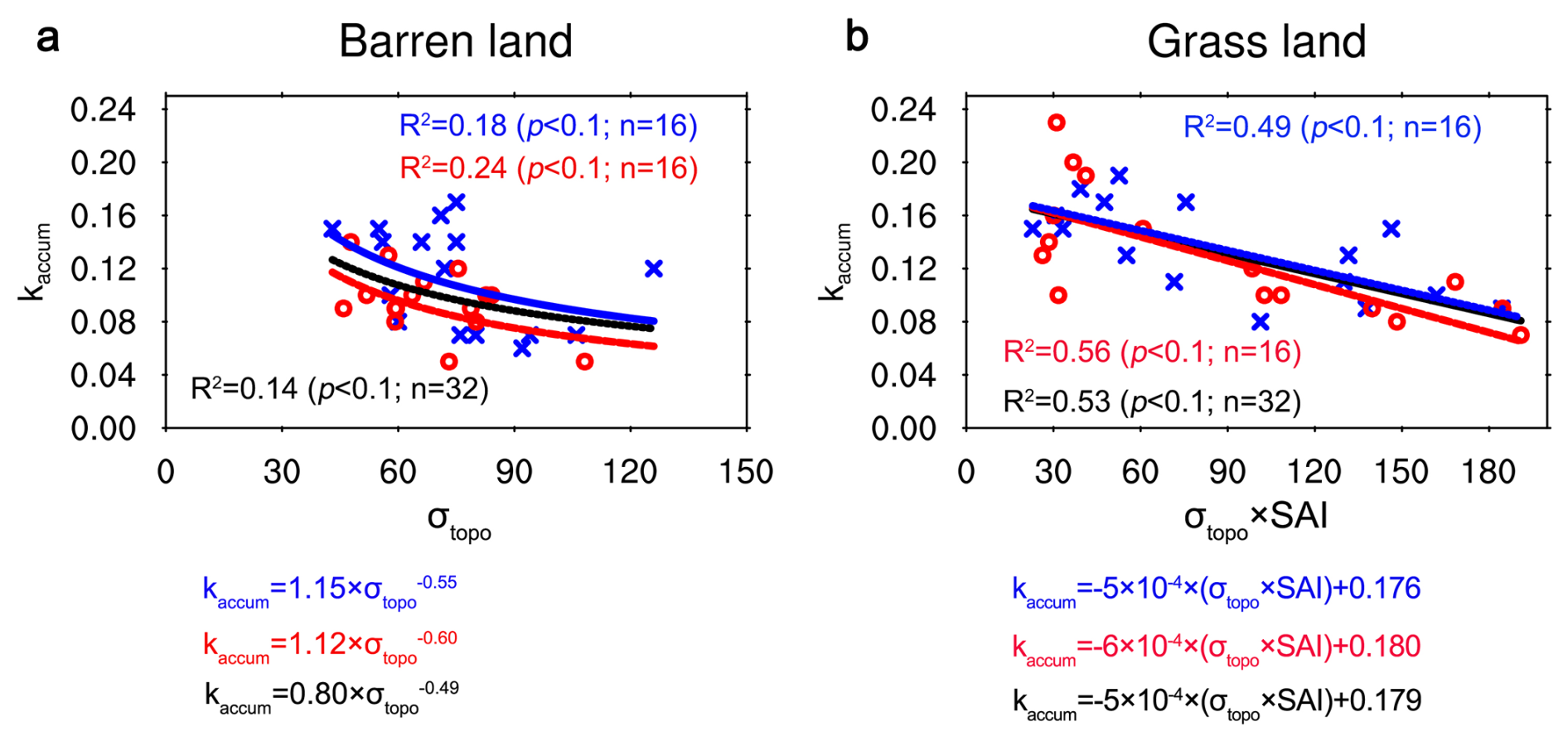
Figure 4 Observed relationship between the optimal value of k_accum (unitless) and σ_topo (m), SAI (unitless) over (a) barren land, (b) grassland based on group 1 (blue crosses) and group 2 (red circles). The blue and red lines represent the fitting results for the samples from group 1 and group 2, respectively, while the black lines represent the fitting results for the combined samples from both groups, with regressed equations marked by the corresponding colour.

Based on a cloud-free MODIS SCF dataset and a snow depth downscaling product (see Sect. 2.1 for details), the observed relationship between SCF and snow depth during snowfall was examined over the selected panels on the TP (Fig. 3). In general, SCF increases with increasing snow depth, consistent with findings from previous studies (e.g., Niu and Yang, 2007; Swenson and Lawrence, 2012). However, the SCF–snow depth relationship varies among panels with different topographic relief (σ_topo) and SAI, highlighting the importance of accounting for underlying surface heterogeneity. To quantify these differences, the optimal values of k_accum were estimated for each of the 32 panels in groups 1 and 2 during snowfall by minimizing the RMSE between the observed and fitted SCF values. The resulting optimal k_accum values are shown in blue and red font in Fig. 3. Over barren land, the optimal k_accum spans from 0.06 to 0.17, k_accum generally decreases with the larger σ_topo, and the averaged optimal k_accum is close to the default value of 0.1. Whereas, over alpine grassland, the optimal k_accum mostly exceeds 0.1, which varies with σ_topo and SAI. Comparison between the optimal k_accum and the default, the original scheme should overestimate the SCF over areas with small σ_topo, while the SCF over the alpine grassland is underestimated. Thus, above results demonstrate the values of k_accum should not be a constant, revealing pronounced spatial differences.

To describe the spatial diversity of k_accum, we further parameterized k_accum through quantifying relationship between the optimal value of k_accum and σ_topo, SAI (Fig. 4). It can be seen that, group 1, group 2 and their combination show similar results, k_accum is represented by a power function depending solely on σ_topo over barren land, while k_accum is calculated by a linear equation that depends on σ_topo×SAI which represents the combined their effects over grass land. The choice of equation for k_accum can also be physically justified. Over barren land, when σ_topo is small (i.e., the ground surface is relatively flat), snowfall is distributed more evenly across the surface, resulting in a relatively high SCF. In contrast, as σ_topo increases (i.e., terrain relief becomes more pronounced), snow tends to accumulate in topographic depressions, leading to a relative decrease in SCF. However, as terrain complexity continues to increase, the suppressing effect of topography on SCF gradually weakens. This is because snow cover over the TP is generally shallow due to limited snowfall, resulting in only minor changes in snow distribution even under highly complex terrain conditions. Over grassland, the probability distribution of snow cover during snowfall is jointly suppressed by both σ_topo and SAI.

The fitted functional forms of the k_accum equations are generally consistent among group 1, group 2, and the combined samples (Fig. 4). Although the estimated coefficients vary somewhat between the fitted relationships, the associated uncertainties in SCF simulations appear to be relatively small and remain within an acceptable range. Finally, we obtained the calculation formula of k_accum over the barren land and grassland as the following equation

$$\begin{array}{}\text{(7)}& k_{\mathrm{accum}}=\left\{\begin{array}{ll}\mathrm{1.15}\times {\mathit{\sigma }}_{\mathrm{topo}}^{-\mathrm{0.55}}& \mathrm{Barren}\mathrm{land}\\ -\mathrm{5}\times {\mathrm{10}}^{-\mathrm{4}}\times \left({\mathit{\sigma }}_{\mathrm{topo}}\times \mathrm{SAI}\right)+\mathrm{0.18}& \mathrm{Grass}\mathrm{land}.\end{array}\right.\end{array}$$

Then, Eq. (7) was combined with Eq. (4) and the optimized SCF parameterization during snowfall was yielded as follows

$$\begin{array}{}\text{(8)}& \begin{array}{rl}& f_{\mathrm{snow}}^{n+\mathrm{1}}=\\ & \left\{\begin{array}{ll}\mathrm{1}-\left(\left(\mathrm{1}-\tanh \left[\left(\mathrm{1.15}\times {\mathit{\sigma }}_{\mathrm{topo}}^{-\mathrm{0.55}}\right)\times q_{\mathrm{snow}}\mathrm{\Delta }t\right]\right)\left(\mathrm{1}-f_{\mathrm{snow}}^n\right)\right)& \mathrm{Barren}\mathrm{land}\\ \mathrm{1}-\left(\left(\mathrm{1}-\tanh \left[\left(-\mathrm{5}\times {\mathrm{10}}^{-\mathrm{4}}\times \left({\mathit{\sigma }}_{\mathrm{topo}}\times \mathrm{SAI}\right)+\mathrm{0.18}\right)\times q_{\mathrm{snow}}\mathrm{\Delta }t\right]\right)\left(\mathrm{1}-f_{\mathrm{snow}}^n\right)\right)& \mathrm{Grass}\mathrm{land}.\end{array}\right.\end{array}\end{array}$$

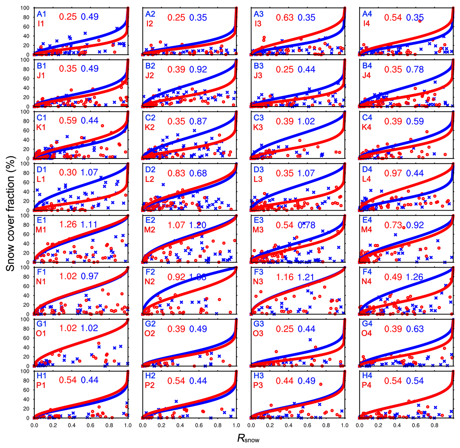
Figure 5 Observed relationship between snow cover fraction (SCF; %) and R_snow (unitless) in 0.1×0.1 grid cells of 32 panels of group 1 (blue crosses) and group 2 (red circles) during snow melt over the TP. The fitted lines are computed from Eq. (5) with the optimal values of N_melt (blue and red font numbers are from group 1 and group 2, respectively) which were estimated when RMSE between observed SCF and fitted value are smallest.

3.3 Revising snow depletion curves by modifying parameterization of the shape parameter (N_melt)

Here, the observed relationship between SCF and R_snow during the snowmelt period was analyzed (Fig. 5). In general, SCF decreases rapidly at the onset of snowmelt (large R_snow). As snowmelt progresses (R_snow becomes small), the rate of SCF depletion gradually slows. The snow depletion curves exhibit distinct shapes across panels with different topographic relief (σ_topo) and SAI, suggesting that both topographic heterogeneity and WGS influence snowmelt processes. The current SCF parameterization scheme (Eqs. 5 and 6) in CLM5 accounts for the effects of topographic relief by assuming that larger σ_topo values lead to faster snow depletion. However, topography can also reduce incoming solar radiation through terrain-shadowing effects over the TP (Zhang et al., 2022), which may act to slow snowmelt in some regions. Furthermore, studies suggested the WGS can warm ground (Domine et al., 2022) and benefit the melting of snow over the TP (Yang et al., 2023; Qi et al., 2024). Therefore, how to explicitly incorporate the influences of pronounced topographic relief and WGS into snow cover parameterizations remains critical.

The shape of snow depletion curve is decided by the parameter N_melt (Fig. 1b). It needs to estimate the optimal value of N_melt over the different underlying surface of TP and revise N_melt parametrization. The optimal value of N_melt was estimated in snowmelt events over each panel of group 1 and group 2 through judging the smallest RMSE between observed SCF and fitted value (blue and red font numbers shown in Fig. 5). We can see that the optimal value of N_melt is obviously smaller than the original value based on the original scheme in CLM5 (Table 1), which means the current scheme should underestimate snow melting rate.

Table 1 Comparison between the optimal N_melt (N_melt,optimal; unitless) and the original N_melt (N_{melt,original} which was calculated from Eq. 6; unitless), and the revised factor (F; unitless) with different σ_topo (m) and SAI (unitless) over barren and grassland.

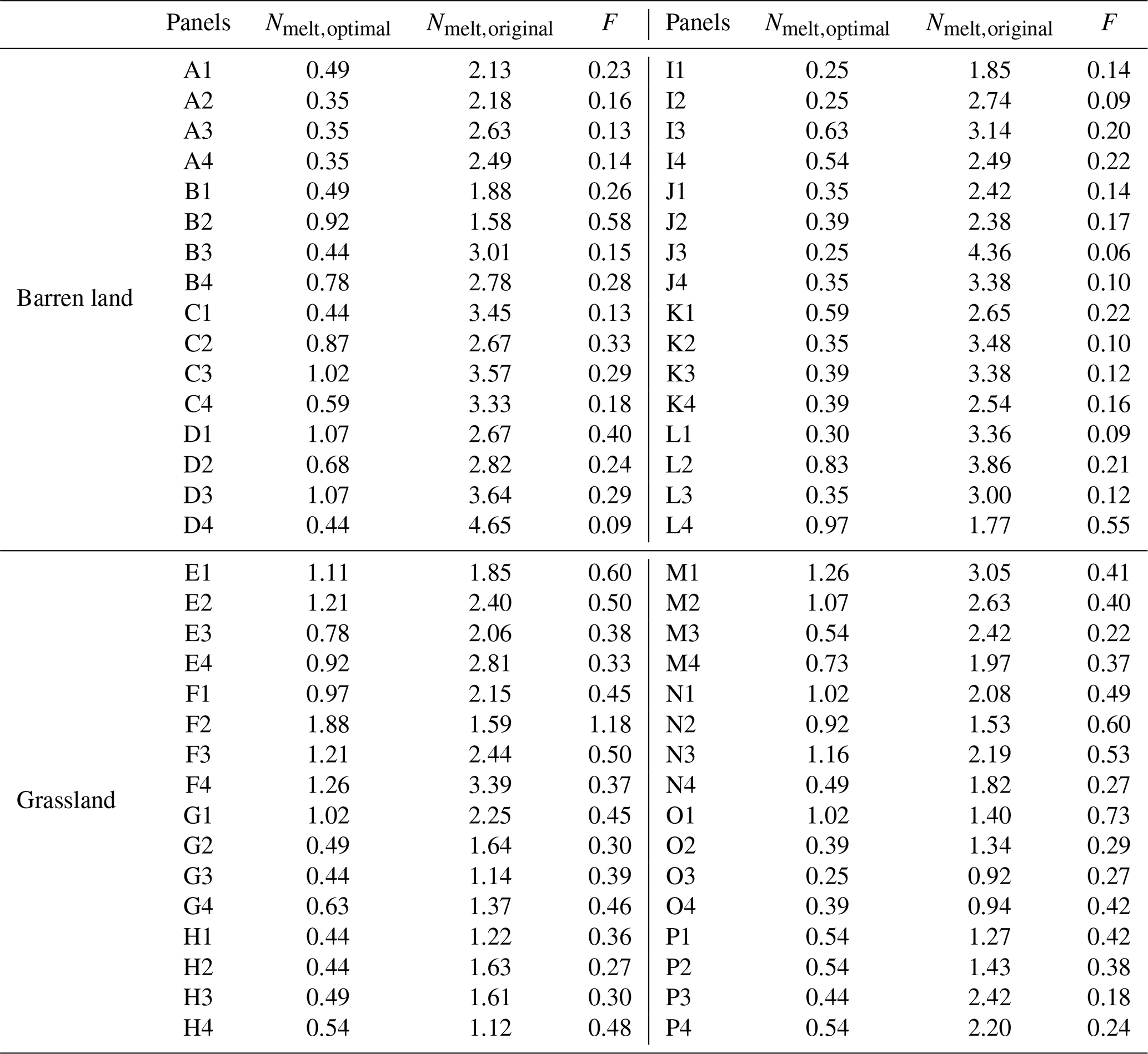
To revise parameterization of N_melt, here, we defined a revised factor F which is calculated as

$$\begin{array}{}\text{(9)}& F=N_{\mathrm{melt},\mathrm{optimal}}/N_{\mathrm{melt},\mathrm{original}}.\end{array}$$

It can be seen that, value of the revised factor F is generally less than 1 (Table 1), which implies lager melting rate over flat barren land and the positive effect of WGS on melting of snow over alpine grassland.

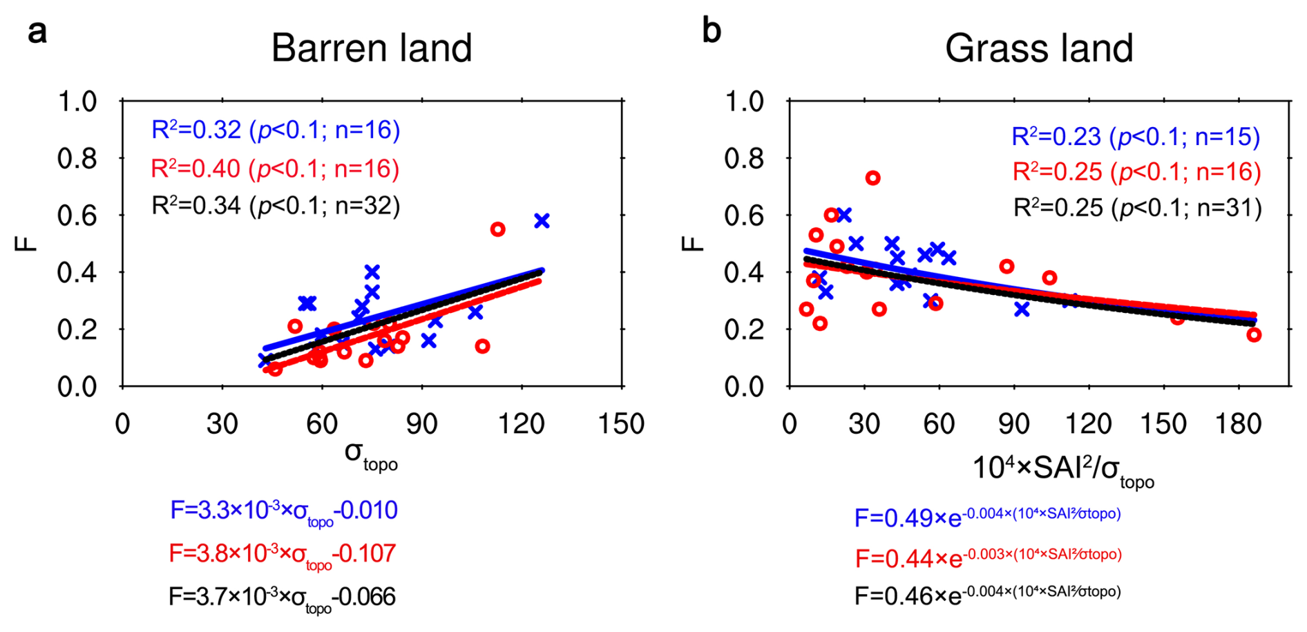
Figure 6 Observed relationship between the revised factor F and σ_topo (m), SAI (unitless) over (a) barren land, (b) grassland based on group 1 (blue crosses) and group 2 (red circles). The blue and red lines represent the fitting results for the samples from group 1 and group 2, respectively, while the black lines represent the fitting results for the combined samples from both groups, with regressed equations marked by the corresponding colour.

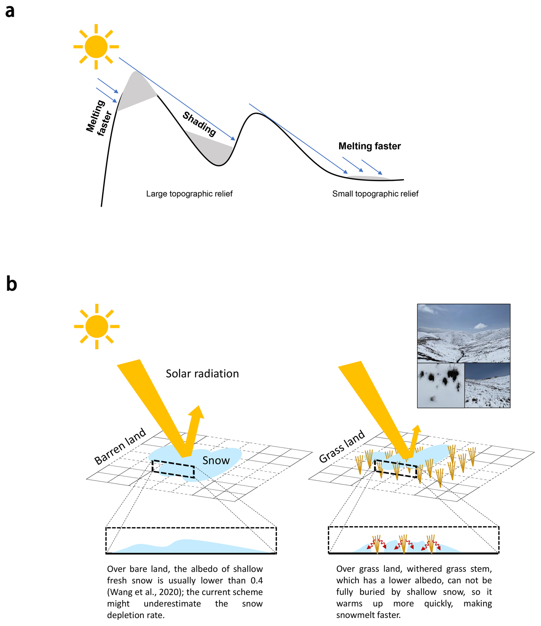
Figure 7 Schematic diagram of topographic relief and short vegetation (i.e., withered grass stems) impacts snowmelt. (a) Illustration of different effects between large and small topographic relief on snowmelt. (b) Comparison of snowmelt between barren land and grassland covered by shallow snow which usually has relatively low albedo (<0.4; Wang et al., 2020).

Relationship between the revised factor F and σ_topo, SAI was further quantified over barren and grassland (Fig. 6). It can be seen that group 1, group 2 and the combined samples yield similar results. Over barren land, F is represented by a linear function of σ_topo, whereas over grassland, F is calculated using an exponential function that depends on ${\mathrm{SAI}}^{\mathrm{2}}/{\mathit{\sigma }}_{\mathrm{topo}}$. Although the parametrization of F was empirically developed based on statistical method, its theoretical basis and the choice of functional form can be physically justified. Over barren land, F increases with larger σ_topo, in other words, snow melt over the flat barren land should be faster than that over the complex topography, which might be due to the effect of topographic shadowing under the patched and shallow snow condition over the TP (Fig. 7a). Over alpine grassland, as SAI increases, F decreases, indicating a negative relationship between F and SAI, implying more WGS can lead to faster snow melt (Fig. 7b), which is consistent with results of previous studies (Domine et al., 2022; Yang et al., 2023; Qi et al., 2024). Considering the additional influence of σ_topo, we further define a factor ${\mathrm{SAI}}^{\mathrm{2}}/{\mathit{\sigma }}_{\mathrm{topo}}$ to represent the combined nonlinear effects of σ_topo and SAI.

The fitted functional forms of the equations for F derived from group 1, group 2 and the combined data (Fig. 6) are generally consistent, despite differences in the fitted coefficients. Thus, to revised N_melt parametrization, effects of topography and WGS were combined to fit the calculation formula of F as follows

$$\begin{array}{}\text{(10)}& {\displaystyle }& {\displaystyle }F=\left\{\begin{array}{ll}{\mathrm{10}}^{-\mathrm{3}}\times \left(\mathrm{3.3}\times {\mathit{\sigma }}_{\mathrm{topo}}-\mathrm{9.5}\right)& \mathrm{Barren}\mathrm{land}\\ \mathrm{0.49}\times e^{-\mathrm{0.004}\times \left({\mathrm{10}}^{\mathrm{4}}\times {\mathrm{SAI}}^{\mathrm{2}}/{\mathit{\sigma }}_{\mathrm{topo}}\right)}& \mathrm{Grass}\mathrm{land}\end{array}\right.\text{(11)}& {\displaystyle }& {\displaystyle }{N}_{\mathrm{melt},\mathrm{revised}}={\displaystyle \frac{\mathrm{200}}{\min \left(\mathrm{10},{\mathit{\sigma }}_{\mathrm{topo}}\right)}}\times F.\end{array}$$

Combining Eqs. (10), (11) with Eq. (5), the optimized SCF parameterization during snowmelt was yielded as follows

$$\begin{array}{}\text{(12)}& \begin{array}{rl}& f_{\mathrm{snow}}=\\ & \left\{\begin{array}{ll}\mathrm{1}-{\left(\frac{{\cos }^{-\mathrm{1}}\left(\mathrm{2}{R}_{\mathrm{snow}}-\mathrm{1}\right)}{\mathit{\pi }}\right)}^{\frac{\mathrm{200}}{\min \left(\mathrm{10},{\mathit{\sigma }}_{\mathrm{topo}}\right)}\times \left[{\mathrm{10}}^{-\mathrm{3}}\times \left(\mathrm{3.3}\times {\mathit{\sigma }}_{\mathrm{topo}}-\mathrm{9.5}\right)\right]}& \mathrm{Barren}\mathrm{land}\\ \mathrm{1}-{\left(\frac{{\cos }^{-\mathrm{1}}\left(\mathrm{2}{R}_{\mathrm{snow}}-\mathrm{1}\right)}{\mathit{\pi }}\right)}^{\frac{\mathrm{200}}{\min \left(\mathrm{10},{\mathit{\sigma }}_{\mathrm{topo}}\right)}\times \left[\mathrm{0.49}\times e^{-\mathrm{0.004}\times \left({\mathrm{10}}^{\mathrm{4}}\times {\mathrm{SAI}}^{\mathrm{2}}/{\mathit{\sigma }}_{\mathrm{topo}}\right)}\right]}& \mathrm{Grass}\mathrm{land}.\end{array}\right.\end{array}\end{array}$$

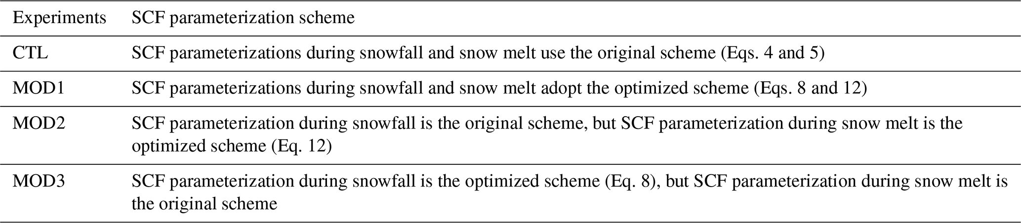
3.4 Experimental design

To evaluate and optimize SCF parameterization, four offline experiments were conducted using CLM5 over the TP (25–40° N, 75–105° E; Fig. 2a) at a spatial resolution of 0.1°×0.1° (Table 2). One is the control experiments (CTL), with SCF parametrizations using the original scheme. The others are the MOD1, MOD2 and MOD3. In MOD1, SCF parametrization adopts the optimized scheme; in MOD2, SCF parameterization only during snow melt adopts the optimized scheme; while in MOD3, SCF parameterization only during snowfall adopts the optimized scheme. Through comparing simulations between MOD1, MOD2 and MOD3, performance of the optimized scheme during snowfall and snow melt can be separately validated. The simulations cover the period from 1979 to 2018, with a model time step of 1800 s and monthly output frequency. The meteorological forcing data were derived from the CMFD v1.6 (see Sect. 2.1 for details). CLM5 was run within the framework of Community Earth System Model (CESM) version 2.2.0 using the I2000Clm50SpGs component set. In this configuration, vegetation canopy properties are prescribed from satellite observations, and the standard crop parameterization is applied without dynamic land-use and land-cover change. The first 23 years (1979–2001) were used for a spin-up to satisfy the model equilibrium, and rest simulations during 2002–2011 used for analysis.

Table 2 Description of experimental design.

4 Results

4.1 Characteristics of CLM5 simulated winter snow cover biases

It has been reported that cold biases are pronounced during winter (Meng et al., 2018), and biases in SCF simulated by CLM are also relatively large during this season (Toure et al., 2016; Ma and Wang, 2022). Given the importance of winter snow cover and its associated modeling uncertainties, this study focuses on the simulation of SCF over the TP during winter. Most regions of the TP are snow covered in winter, and snow is distributed in a patchy and fragmented manner, with SCF generally below 50 % over most areas at the grid-cell scale (10×10 km) (Fig. 8a). Except for the southeastern TP (e.g., the Nyenchen Tanglha Mountains), snow cover over the TP is generally shallow, with snow depth around or less than 10 cm (Fig. 8b). Nevertheless, most LSMs exhibit poor performance in simulating such fragmented and shallow snow cover over the TP, typically overestimating snow extent (Toure et al., 2016; Orsolini et al., 2019). In contrast, CLM5 shows relatively small SCF biases over the eastern and southwestern TP, while pronounced biases occur over the northwestern TP, the Kunlun Mountains, the Bayan Har Mountains, and the Siguniang Mountains (Fig. 8c and e). Specifically, positive SCF biases dominate the western and central TP, whereas negative biases are evident over the southeastern TP. The spatial correlation coefficients (R) of SCF over both grassland and barren land exceed 0.5, indicating that CLM5 is generally capable of reproducing the spatial distribution of winter SCF over the TP. However, the regionally averaged MEB and RMSE of SCF remain relatively large. Over the entire TP, grassland, and barren land, the MEB (RMSE) values are 9.79 % (21.71 %), 3.37 % (16.33 %), and 13.13 % (23.20 %), respectively (Table 3).

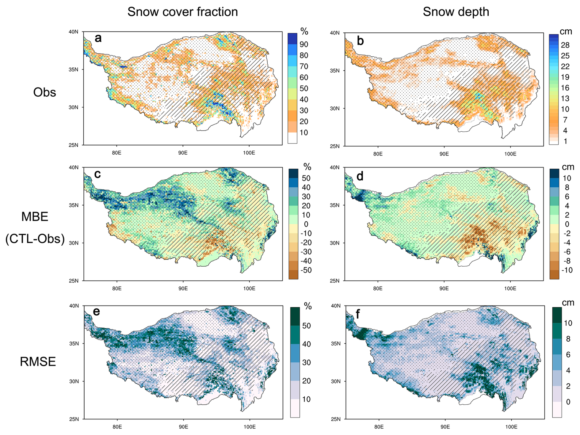
Figure 8 Distribution of winter (DJF mean) snow cover and CLM5 simulation biases. Observed (Obs) 2003–2012 averaged DJF (a) snow cover fraction (SCF; %), (b) snow depth (cm). CLM5 mean bias error (MEB; CTL-Obs) of (c) SCF, (d) snow depth during period 2003–2012. In each panel, slash shading and dot shading represent grassland and barren land, respectively. (e) and (f) are same as (c) and (d) but for RMSE.

Table 3 Comparison of winter SCF simulation MBE (%), RMSE (%) and R (unitless) between the CTL and MOD1, MOD2, MOD3.

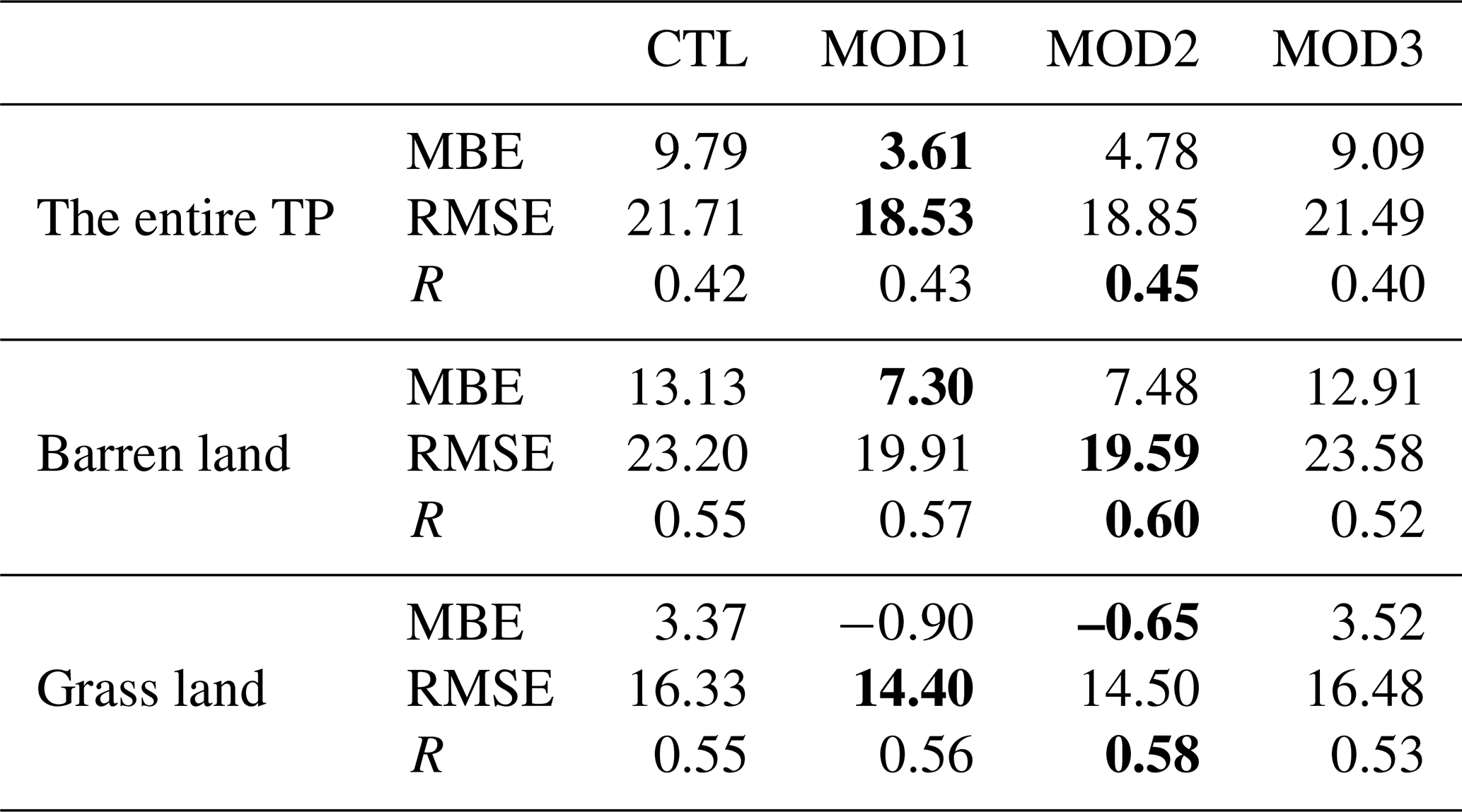
Note: the bold black values are the lowest MBE, lowest RMSE and largest R among the CTL, MOD1, MOD2 and MOD3.

SCF generally increases with the thicker snow depth, therefore, biases in SCF may be related to biases in snow depth. Indeed, the spatial pattern of snow depth biases (Fig. 8d and f) is broadly consistent with that of SCF. but the northwestern TP does not exhibit correspondingly large snow depth biases, suggesting that the pronounced SCF biases in this region are mainly attributable to deficiencies in the SCF parameterization in CLM5. Overall, CLM5 tends to overestimate winter snow cover over the TP, indicating that the SCF parameterization requires further optimization.

4.2 Preliminary validation of the optimized SCF parameterization scheme

The details of the SCF parameterization scheme optimization by considering the impacts of WGS and topography have been introduced in Sect. 3.2 and 3.3. Based on this framework, a preliminary validation of the optimized SCF parameterization was conducted. As shown in Fig. 9a, d, and g, the optimized SCF scheme (MOD1) markedly improves the simulation of winter SCF by reducing both MEB and RMSE. The most substantial improvements occur over the northwestern TP, the Kunlun Mountains, Bayan Har Mountains, and Siguniang Mountains, where the original scheme substantially overestimates SCF. The optimized scheme also moderately reduces the negative SCF biases over the southeastern TP, whereas its influence remains limited in the southwestern TP, particularly over the Himalayan Mountains. Consequently, the regionally averaged MEB (RMSE) of SCF over the entire TP, grassland, and barren land is reduced to 3.61 % (18.53 %), −0.9 % (14.40 %), and 7.30 % (19.91 %), respectively (Table 3). Compared with CTL, the optimized scheme simulates less SCF over the barren and mountainous areas where the original scheme has obvious positive biases, and more SCF over the southeastern TP where the original scheme has negative biases. The positive biases of winter SCF are relatively reduced by 63 % ($[{\mathrm{MEB}}_{\mathrm{MOD}\mathrm{1}}-{\mathrm{MEB}}_{\mathrm{CTL}}]/{\mathrm{MEB}}_{\mathrm{CTL}}\times \mathrm{100}\mathit{\%})$ over the entire TP. Over the grassland and barren land used for optimizing SCF parameterization, winter SCF simulation MBE from the MOD2 are also obviously smaller than that of the CTL (Fig. 9b and e).

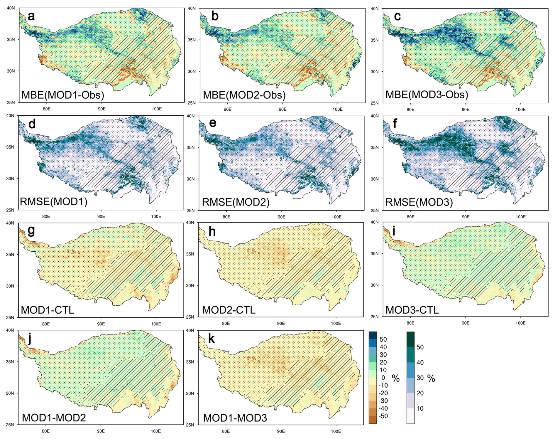
Figure 9 Comparison of simulations of SCF with modified scheme (MOD1, MOD2, MOD3) with observation (Obs) and simulations with current scheme (CTL). Mean bias error (MBE) of SCF from experiments (a) MOD1, (b) MOD2, (c) MOD3. Root mean square error (RMSE) of SCF from experiment (d) MOD1, (e) MOD2, (f) MOD3. Differences of SCF between (g) MOD1 and CTL, (h) MOD2 and CTL, (i) MOD3 and CTL, (j) MOD1 and MOD2, (k) MOD1 and MOD3.

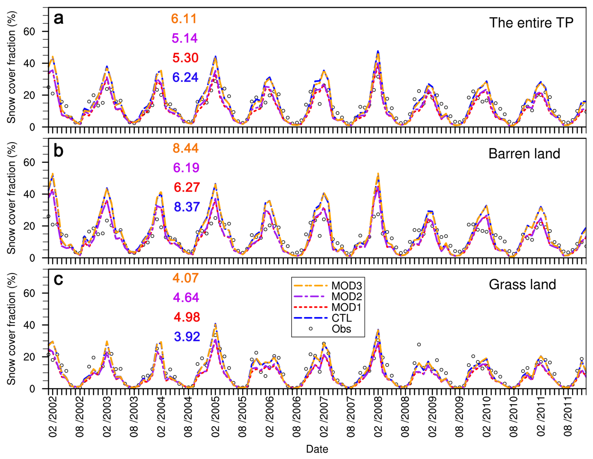
Figure 10 Comparison of simulated snow cover fraction (SCF; %) with observation during 2002–2011. Evolution of SCF averaged (a) the entire TP, (b) barren land, (c) grassland. The coloured values represent the RMSE of SCF for the corresponding experiments.

In CLM5, SCF during snowfall and snowmelt periods is calculated separately. Therefore, the improvements shown in the MOD1 experiment represent the combined effects of the optimized SCF scheme during both periods. To further identify which process contributes most to the improvement, simulations using the optimized SCF scheme only during the snowmelt period (i.e., the MOD2 experiment) are compared with CTL (Fig. 9h). MOD2 simulates lower SCF than the CTL over most regions of the TP, except for some areas with large topographic relief in the southern TP, thereby reducing the positive SCF biases. Quantitatively, MEB of SCF averaged over the entire TP, grassland, and barren land decreases to 4.78 %, −0.65 %, and 7.48 %, respectively. Although the regionally averaged reduction in SCF biases is slightly smaller in MOD2 than that in MOD1, the spatial pattern of SCF differences between the two experiments (Fig. 9j) indicates that MOD2 achieves larger bias reductions across most of the TP, with the exceptions of the Pamir Mountains and the Siguniang Mountains, where the improvements are greater in MOD1. This indicates that the overall improvements achieved by the optimized SCF scheme are primarily attributable to the modifications during the snowmelt process. In the optimized SCF parameterization for the snowmelt period, the shape parameter (N_melt) is modified by multiplying a revised factor (F) that is less than 1. A smaller N_melt corresponds to a faster snow depletion rate during snowmelt (Fig. 1b), which effectively reduces the positive SCF biases. In other words, the original SCF scheme underestimates the snow depletion rate, particularly over flat barren land, and the optimized scheme alleviates this deficiency to a considerable extent. Simulations using the optimized SCF scheme only during snowfall events (i.e., the MOD3 experiment) result in only marginal improvements over barren land (Fig. 9c, f, i, and k), with the regionally averaged SCF MEB decreasing to 12.91 %. In contrast, SCF biases over grassland become slightly larger in MOD3. This difference may be attributed to the presence of WGS, which acts as a physical barrier that inhibits wind-driven snow transport into topographic depressions. As a result, snow tends to be retained more effectively over grassland than over barren land, leading to higher SCF values. For the optimized SCF parameterization scheme during snowfall, the values of the probability distribution coefficient (k_accum) can be greater than 1 (the default value in the original scheme) over areas with small σ_topo and SAI (Fig. 4), which means the SCF during snowfall over the flat and sparse vegetation areas calculated by the optimized scheme is larger than that of the original scheme, but smaller over the large topographic relief area. Overall, the optimized SCF has the potential to more comprehensively account for the effects of underlying surface heterogeneity and improve the representation of the physical processes governing SCF variations.

We further validated simulations in SCF evolution during period 2002–2011 (Fig. 10). In CTL experiment (i.e., original scheme), seasonal and interannual variations of SCF simulated by CLM5 generally agree with the observations over the TP (Fig. 10a). However, winter SCF is consistently overestimated, resulting in a RMSE of 6.24 %. In contrast, the optimized scheme (MOD2) shows much better agreement with the observations, reducing the RMSE to 5.14 %. Over barren land, the winter overestimation of SCF in the CTL experiment is more pronounced (Fig. 10b). The optimized scheme effectively alleviates this positive bias, reducing the RMSE from 8.37 % to 6.19 %. Over grassland, the SCF biases simulated by CLM5 are relatively small, with an RMSE of approximately 4 % (Fig. 10c). The optimized scheme leads to a slight deterioration in performance over grassland, which may be attributable to the reduction in winter SCF causing a modest underestimation during the snowmelt period from April to June.

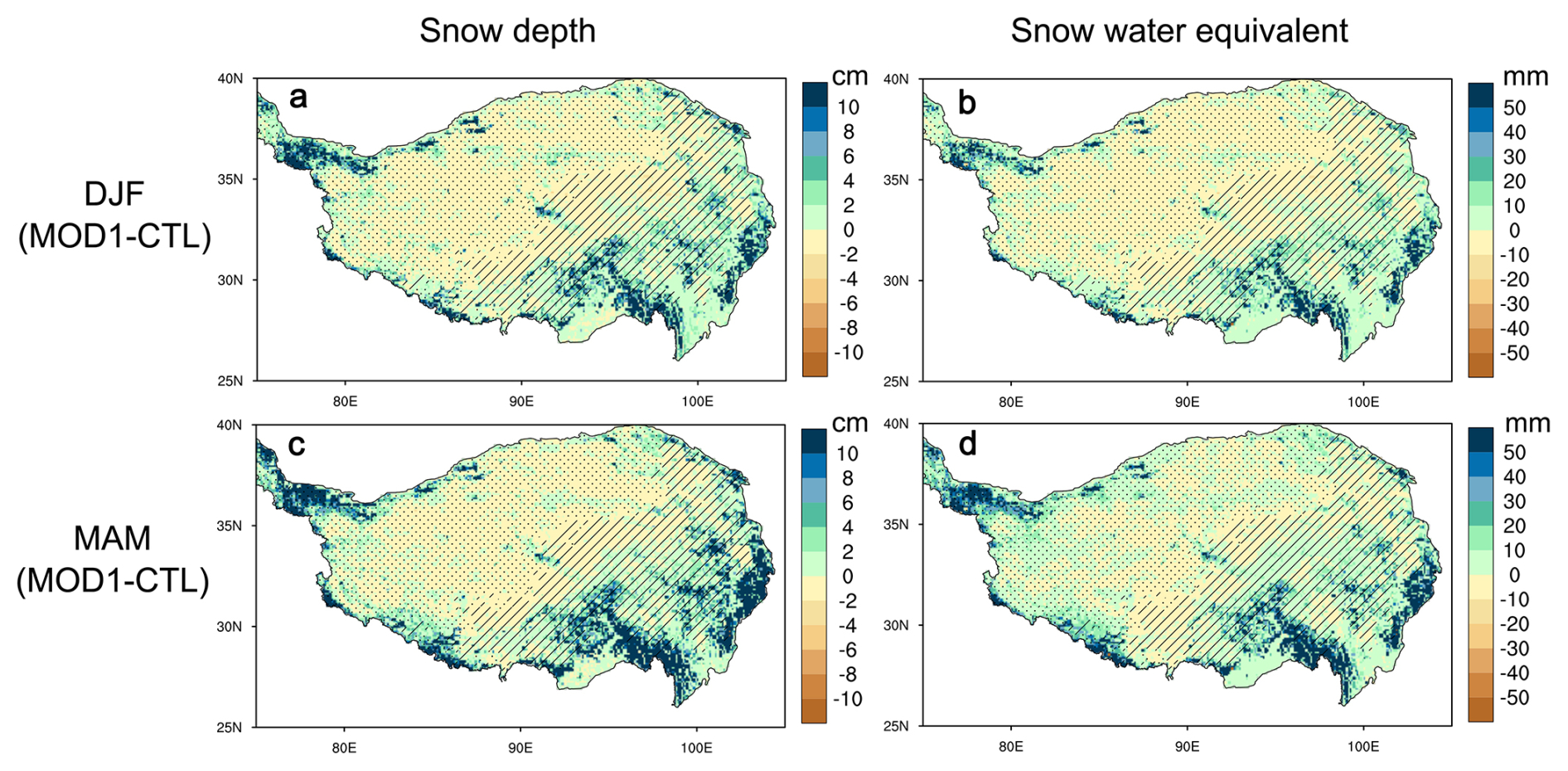
Figure 11 Differences of gridcell mean snow depth (cm) and snow water equivalent (mm) between MOD1 and CTL during winter (DJF) and spring (MAM).

To assess the impacts of the optimized SCF scheme on snow mass simulations, Fig. 11 shows the differences in snow depth and snow water equivalent (SWE) between the MOD1 and CTL experiments during winter and spring. The optimized SCF scheme generally leads to greater snow depth than the original scheme in both seasons (Fig. 11a and c). This is attributable to the snow accumulation formulation in CLM5, where the increase in snow depth is determined by snowfall divided by SCF. Therefore, a lower SCF results in a larger snow depth increment for the same snowfall amount. The optimized scheme likewise produces higher SWE values than the original scheme (Fig. 11b and d).

4.3 Effects of the optimized scheme on the surface energy budget

SCF is an important factor influencing the surface albedo. As shown in Fig. 12a, the observed surface albedo ranges from 0.1 to 0.8, with relatively high values occurring over the eastern TP. CLM5 generally captures the spatial distribution of surface albedo, yielding a spatial correlation coefficient (R) of 0.63. However, due to the overestimation of SCF, CLM5 has obvious positive biases of surface albedo by up to 0.3 (Fig. 12b), especially over the northwestern TP. And the spatial pattern of surface albedo bias is similar to that of SCF, which further confirm that winter SCF bias should be the main cause of the surface energy budget bias. While the optimized SCF scheme simulated lower surface albedo than that of the original scheme (Fig. 12c), especially over the northern TP where SCF simulation is obviously improved, difference of surface albedo between MOD1 and CTL can be about −0.1, thus, the positive biases in surface albedo are obviously reduced, and the optimized SCF scheme also improves the simulation of the spatial distribution of winter surface albedo by CLM5, with R increasing to 0.65., despite the remaining positive surface albedo bias in MOD1, which may be attributed to unresolved SCF biases and other process imperfections (such as snow albedo estimation).

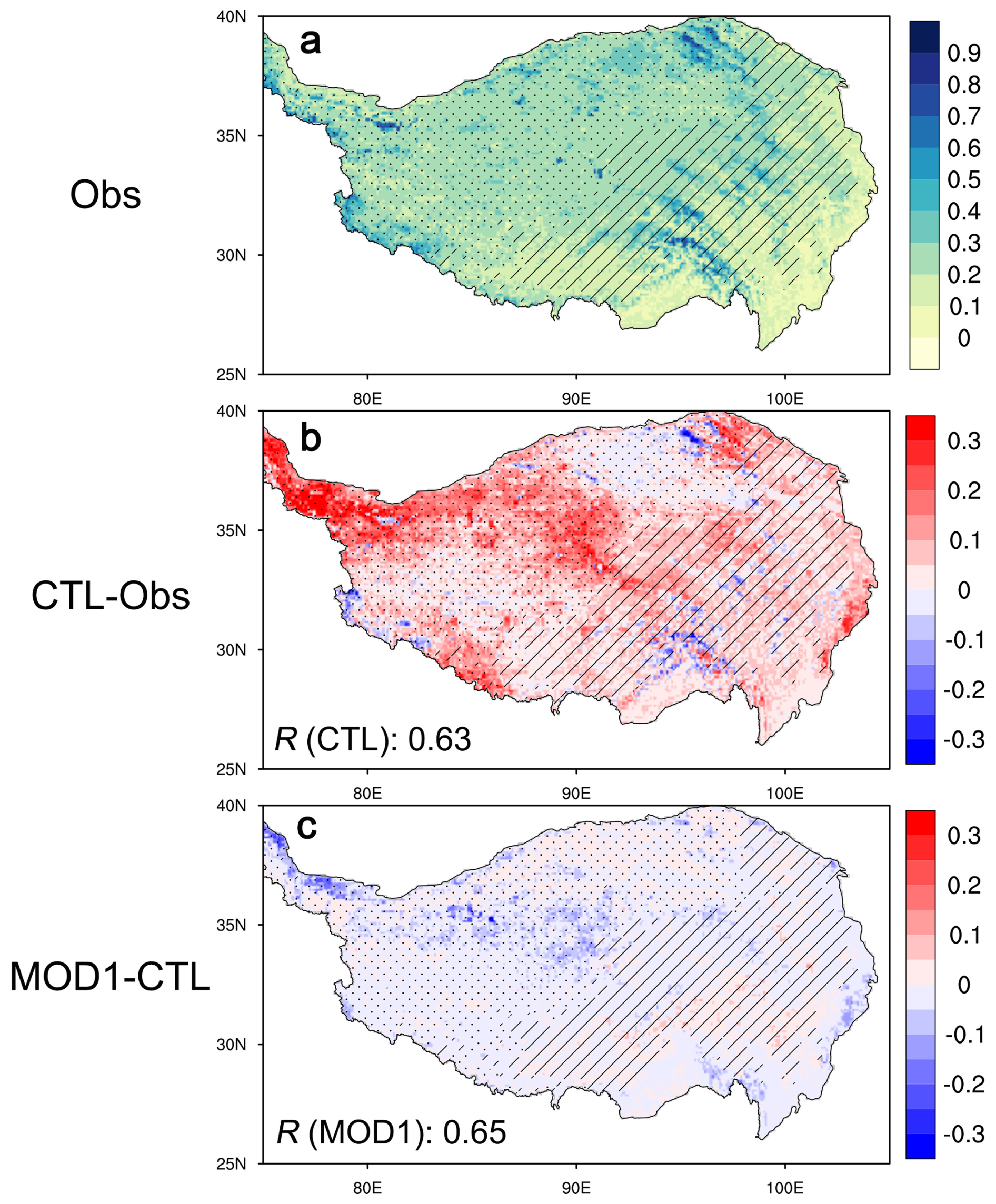
Figure 12 Comparison of simulations of winter surface albedo (unitless) by the modified scheme (MOD1) and current scheme (CTL) with observation (Obs) over the TP. (a) Spatial distribution of surface albedo from MODSI observation. (b) Differences between CTL and Obs. (c) Differences between MOD1 and CTL. The values in (b) and (c) are the spatial correlation coefficient of CTL, MOD1 experiments with Obs.

Improvements in surface albedo simulation further affect the simulation of the surface energy budget. Compared with the original scheme (CTL experiment), the optimized SCF scheme (MOD1 experiment) produces a lower surface albedo, resulting in a substantial increase in net shortwave radiation at the surface (Fig. 13a). Consequently, both net longwave radiation and sensible heat flux increase (Fig. 13b and c), and the spatial patterns of their differences between MOD1 and CTL generally correspond to those of net shortwave radiation. In contrast, the latent heat flux simulated by the optimized SCF scheme decreases slightly (Fig. 13d), likely due to the reduced snow-covered area and decreased snow sublimation during winter. The impact on ground heat flux is relatively small (Fig. 13e).

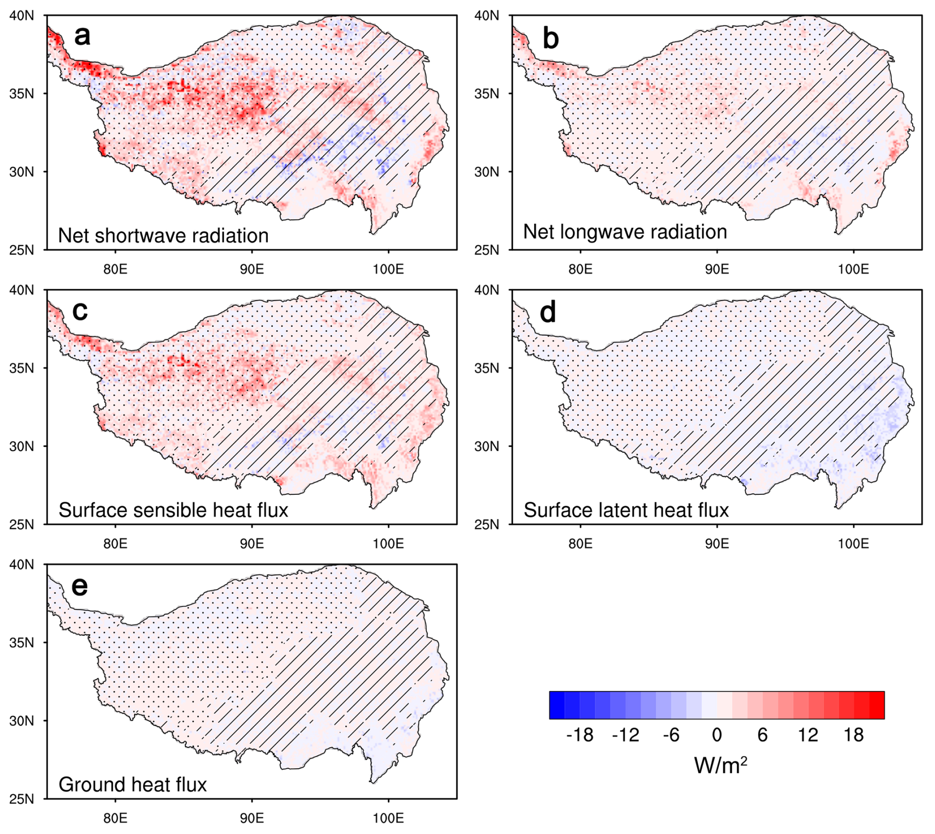
Figure 13 Differences of surface energy budget (W m⁻²) between MOD1 and CTL during winter. (a) Net shortwave radiation, (b) net longwave radiation over land surface. (c) surface sensible heat flux, (d) surface latent heat flux, (e) ground heat flux.

Surface energy budget further influences the land surface temperature (LST). The observed LST exhibits a pronounced spatial pattern, with colder temperatures generally occurring at higher elevations (Fig. 14a). CLM5 generally reproduces the overall spatial distribution of winter LST over the TP, with a spatial correlation coefficient  R) of 0.55. Nevertheless, it has been reported that, current climate models have obviously cold biases over the TP (Orsolini et al., 2019; Zhou et al., 2023), which is one of the main causes of uncertainties in simulations and projection of permafrost degeneration, surface hydrology and ecology, as well as understanding the TP thermal forcing (Yang et al., 2019; Ehlers et al., 2022). As excepted, CLM5 still shows cold biases over most regions of TP (Fig. 14b), especially over northern TP where snow cover fraction is overestimated and southeastern TP. Compared to the original scheme, the optimized SCF scheme simulated the warmer LST (Fig. 14c), in other words, the optimized SCF scheme reduces the cold bias.

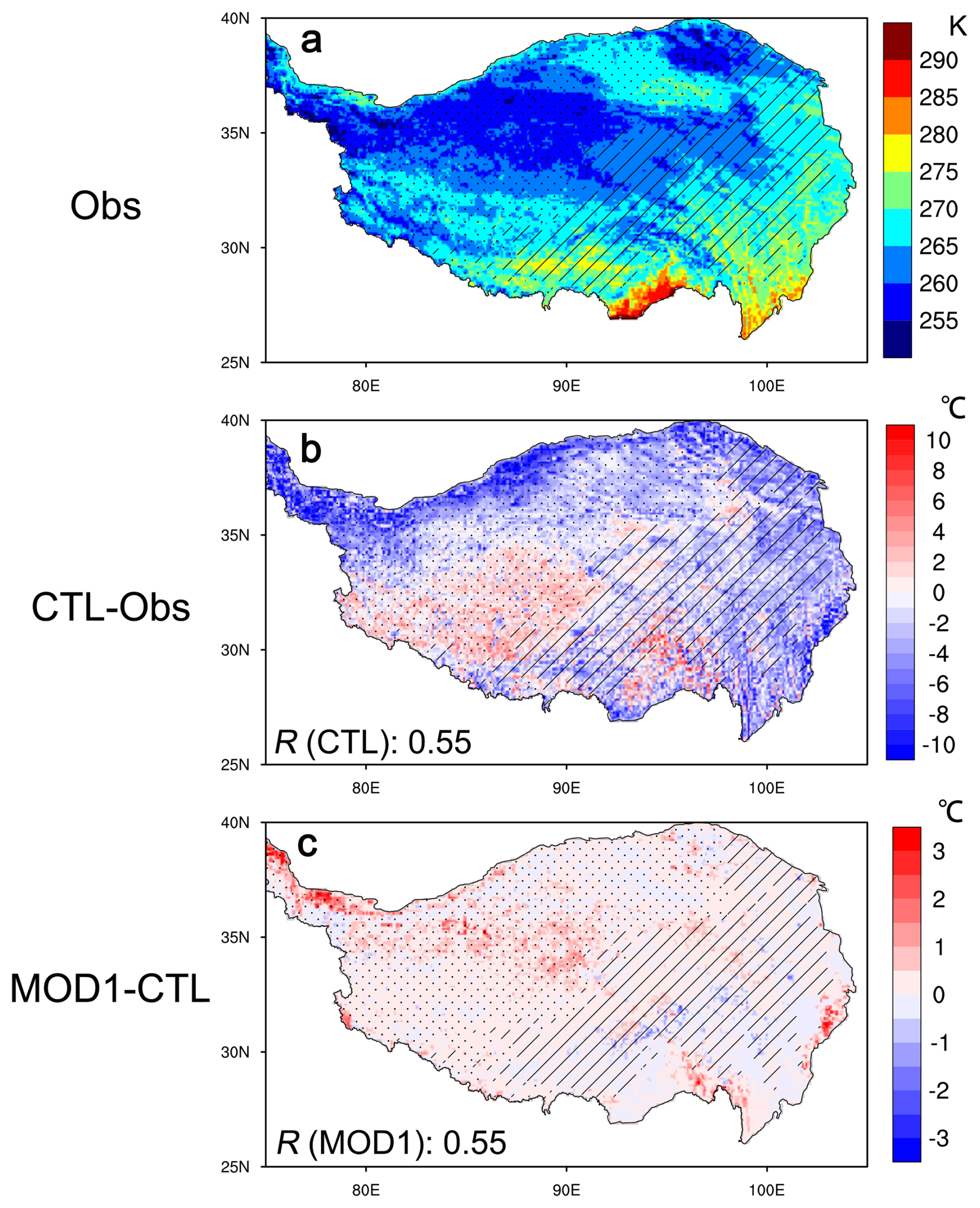
Figure 14 Comparison of simulations of winter land surface temperature (LST) by the modified scheme (MOD1) and current scheme (CTL) with observation (Obs) over the TP. (a) Observation of LST (K) from MODSI. (b) Differences (°C) between CTL experiment and Obs. (c) Differences of between MOD1 and CTL experiments. The values in (b) and (c) are the spatial correlation coefficient of CTL, MOD1 experiments with Obs.

Overall, the optimized SCF scheme not only improves the winter SCF simulation over the TP, but also optimizes simulations of the surface energy budget to some extent.

5 Discussions

5.1 Uncertainties in the meteorological forcing dataset and the parameterization of total precipitation partitioning into snowfall

It has been widely recognized that biases in meteorological forcing datasets represent an important source of uncertainty in land surface process simulations (e.g., Wang et al., 2016; Zeng et al., 2021; Zhang et al., 2025), including snow cover simulations (Xie et al., 2017; Jiang et al., 2020). The formation and evolution of snow mass on the land surface involve a series of complex processes, including snowfall, accumulation, compaction, aging, and melting. In this study, we primarily focus on improving the parameterization of SCF during snowfall and snowmelt processes. Snow compaction and aging mainly affect snow albedo, which in CLM5 is simulated using the Snow, Ice, and Aerosol Radiative (SNICAR) model. At present, snowfall input to LSMs is diagnosed through parameterization schemes that partition total precipitation into rainfall and snowfall. On the one hand, due to the sparse observational network and uncertainties in reanalysis datasets over the TP, total precipitation in meteorological forcing datasets inevitably contains biases (Liu et al., 2025). These uncertainties may contribute to the remaining snow cover biases, even after optimizing the SCF parameterization. In this study, we adopt the CMFD v1.6. Although a newer version, CMFD v2.0, has recently been released with substantial improvements – including precipitation directly derived from the TPHiPr dataset (Jiang et al., 2023) – previous evaluations indicate that CMFD v1.6 exhibits relatively lower biases compared to other forcing datasets (Liu et al., 2025). Nevertheless, a systematic assessment of the impacts of different meteorological forcing datasets on snow cover simulations over the TP remains necessary and should be addressed in future studies.

On the other hand, the parameterization scheme used to partition total precipitation into snowfall also exerts a strong influence on snow cover simulations. At present, most LSMs estimate the fraction of snowfall in total precipitation using empirical functions that rely primarily on near-surface air temperature as the independent variable. Previous studies (e.g., Leroux et al., 2023; Jennings et al., 2025) have demonstrated that the choice of precipitation phase partitioning scheme constitutes a major source of model sensitivity in simulating changes in snow mass. In CLM5, the partitioning of total precipitation into snowfall and rainfall is diagnosed using a linear ramp function. For most land units, this scheme produces all snowfall at temperatures below 0 °C, all rainfall above 2 °C, and a mixture of snowfall and rainfall at intermediate temperatures. Consequently, improving snowfall estimation in LSMs from alternative perspectives – such as incorporating crowdsourced observations of precipitation phase through data assimilation – may provide a promising pathway for further reducing uncertainties in snow cover simulations (Jennings et al., 2025).

Besides, interaction between snow cover and snowfall, air temperature are complex through snow cover-albedo-radiation energy feedbacks. Improved simulation of snow cover over the TP can effectively help alleviate the cold bias during the cold season (Zhou et al., 2023). In this study, the optimized SCF scheme was evaluated only through offline CLM5 simulations. To more comprehensively assess its impacts on climate simulations, coupled atmosphere–land experiments should be conducted in future studies.

5.2 Remaining challenge for describing the complexity of topographic relief and vegetation diversity

Due to the complexity of the underlying surface, characterized by large topographic relief and diverse vegetation, land surface modeling over the TP remains a challenging task, particularly for snow cover simulations. Over past decades, the development of LSMs has increasingly aimed to represent multiscale land surface processes in a more comprehensive manner (Prentice et al., 2015; Lu et al., 2020). In this study, the impacts of short vegetation (i.e., withered grass stems, WGS) and topography on snow cover are considered only at the grid-cell mean scale. In reality, the influence of topographic relief on snow cover is highly complex, involving both mechanical and radiative processes. Mechanical processes are manifested through snow redistribution and drifting, whereby snow tends to accumulate in gullies and depressions during snowfall. Radiative processes arise from terrain-induced three-dimensional radiation transfer, which generally leads to faster snowmelt on sun-facing slopes, while snow on shaded slopes persists for longer periods. At present, CLM5 accounts for wind effects on fresh snow density at the grid-cell scale but does not explicitly represent three-dimensional terrain radiative effects. Recent studies have demonstrated that incorporating three-dimensional terrain effects is crucial for accurately simulating land surface processes over the TP (e.g., Wang et al., 2020; Miao et al., 2022). Similarly, the influences of short vegetation on snow cover, through mechanical blocking, canopy radiative transfer, and heat conduction between vegetation stems or withered components and the snowpack, primarily operate at subgrid scales. However, the lack of high-resolution datasets describing non-growing-season vegetation poses a major limitation for explicitly representing these processes in current LSMs. Consequently, how to more realistically describe the combined complexity of topographic relief and vegetation diversity remains an open challenge and warrants further investigation in future studies.

5.3 Generality and potential applicability of the optimized SCF parameterization scheme

In this study, the TP was selected as a representative region for optimizing the SCF parameterization scheme under conditions characterized by shallow snow cover and low-stature vegetation. Although developed for the TP, the optimized scheme exhibits a certain degree of generality and may be applicable to other regions with similar environmental characteristics, particularly those featuring complex topography, shallow snow cover, and short vegetation (e.g., grasses and shrubs), whose stems, branches, and senescent plant material are not completely buried by snow.

6 Conclusions

In this study, we evaluated the performance of CLM5 in simulating winter snow cover over the TP, the original SCF parameterization scheme in CLM5 overestimates winter snow cover fraction over the TP, especially over the western TP. One of the main causes is the overlooking the varied probability distribution of snow over different land surface types and underestimating the snow depletion over barren land in the original SCF parameterization scheme. Then, we optimized the SCF parameterization scheme through considering impacts of the WGS and topography to parameterize the probability distribution factor (k_accum) instead of the constant value, revise the depletion curve shape parameter (N_melt). The optimized SCF scheme obviously reduces the winter SCF simulation positive biases by 63 % over the entire TP. Correspondingly, simulations in surface albedo and surface radiation budget are also improved. Results in this study provide a reference way for LSMs development over the TP, which also has potential for improving local and East Asian weather and climate simulations and predictions.