A novel ALE scheme with the internal boundary for coupling tectonic and surface processes in geodynamic models

Recent advancements in modelling the deformation of the Earth's crust and upper mantle, coupled with surface processes, have significantly deepened our understanding of how the Earth responds to integrated tectonic and erosional forces, which are intricately linked to climate dynamics. This study presents a novel coupling framework within the Arbitrary Lagrangian–Eulerian with Internal Boundary (ALE-IB) scheme, which integrates the geodynamic codes Underworld 2 with the surface process code Badlands. Our innovative approach addresses the limitations of previous Eulerian-based coupling frameworks by maintaining the integrity of internal interfaces and providing precise surface tracking. This ensures accurate representation of material boundaries and enhances the fidelity of simulations involving complex geological processes. We detail the principles underlying the coupling of surface processes with tectonic deformation, leveraging the strengths of the ALE-IB scheme to model free surfaces and moving boundaries effectively. By comparing our model's performance with an Eulerian-based approach, we highlight key differences in structural and dynamic behaviour under varying surface process intensities. This comparison offers valuable insights into the intricate interactions between surface and deep Earth processes. Our findings contribute to a more comprehensive understanding of geomorphological and tectonic evolution, providing a robust framework for future research in geodynamic and climate-related geological studies.

1 Introduction

In recent years, modelling the deformation of the Earth's crust and upper mantle, coupled with surface processes, has significantly advanced our understanding of how the Earth responds to integrated tectonic and erosional forcing, which are linked to climate dynamics (Willett et al., 1993; Batt and Braun, 1997; Beaumont et al., 2001; Braun et al., 2008). The development of these models has evolved from one-way coupling frameworks to fully two-way coupled systems. Additionally, modelling has progressed from limited two-dimensional analyses to three-dimensional approaches that consider more complex interactions, especially with free upper surfaces.

Initially, researchers constructed one-way coupled models by incorporating simple surface processes into two-dimensional tectonic frameworks (Kooi and Beaumont, 1994; Avouac and Burov, 1996; Beaumont et al., 1996; Batt and Braun, 1997, 1999; Willett, 1999; Pysklywec, 2006; Kaus et al., 2008). Some studies implemented tectonics through prescribed displacement functions and modelled isostatic responses within Landscape Evolution Models (LEMs) (Beaumont et al., 1992; Kooi and Beaumont, 1996; Tucker and Slingerland, 1996; Densmore et al., 1998). In recent years, fully coupled three-dimensional dynamic models – integrating 3-D tectonic simulations with 2-D surface process models – have emerged (Kurfeß and Heidbach, 2009; Maniatis et al., 2009; Braun and Yamato, 2010; Collignon et al., 2014; Thieulot et al., 2014; Ueda et al., 2015; Schröder, 2016; Roy et al., 2016; Nettesheim et al., 2018; Beucher et al., 2019; Neuharth et al., 2022; Wolf et al., 2022). These advanced models are capable of accounting for large stresses arising from surface topography gradients and complex interactions between surface and deep earth processes.

The accuracy and efficiency of coupled models strongly depend on the underlying framework used to construct the tectonic and surface process models, as well as the communication between these components. Existing models vary considerably because each is tailored to specific tectonic scenarios, incorporating different thermo-mechanical models and surface process schemes (Ueda et al., 2015). Many of these models employ the Arbitrary Lagrangian–Eulerian (ALE) or Eulerian descriptions of flow fields, utilizing particle-in-cell or level-set methods to trace material interfaces within finite element or finite difference frameworks (Braun and Yamato, 2010; Collignon et al., 2014; Thieulot et al., 2014; Ueda et al., 2015; Beucher et al., 2019; Wolf et al., 2022). A variety of surface process models are also integrated, such as Cascade (Braun and Sambridge, 1997), CHILD (Tucker et al., 2001), FastScape (Braun and Willett, 2013), DAC (Goren et al., 2014), and Badlands (Salles, 2016), each designed to address specific aspects of surface evolution. Given the diversity of model choices and input parameters, it is essential to evaluate the dependence of results on these factors through systematic benchmarking of coupled models.

Regarding the flow dynamics framework, the Eulerian description, combined with particle-in-cell methods, often lacks precise tracking of surfaces and velocities at the Earth's surface. In contrast, ALE methods offer advantages in modelling free surfaces and moving boundaries, thus providing a superior framework for surface-tectonic coupling. The ALE with the internal boundary (ALE-IB) further enhances the ALE approach by maintaining the integrity of internal interfaces (Lu et al., 2026), preventing numerical artifacts, and improving solution stability. It explicitly enforces physical conditions, such as stress and displacement jumps, at internal boundaries during mesh movement, which is especially important for accurately representing different material types (e.g. crust, sediments, ice, water, air) and their transportation through the Earth's surface.

In this paper, we present a novel coupling framework that integrates the geodynamic codes Underworld 2 (Moresi et al., 2007; Mansour et al., 2020) with the surface process code Badlands (Salles, 2016; Salles and Hardiman, 2016; Salles et al., 2018) within the ALE-IB scheme. First, we outline the modelling approach and detail the principles underlying the coupling between surface processes and tectonic deformation. Second, we compare the performance of the coupled model built within this framework to that of an Eulerian-based approach, examining differences in structural and dynamic behaviour under varying surface process intensities.

2 Method

2.1 Tectonic and surface processes modelling

2.1.1 Underworld 2

For the tectonic modelling, we use the particle-in-cell and finite element method (FEM-PIC) code Underworld 2 (Moresi et al., 2007; Mansour et al., 2020) to simulate the long-term deformation of the lithosphere by solving a set of equations covering momentum, mass and heat conservation:

$$\begin{array}{}\text{(1a)}& {\displaystyle }& {\displaystyle }\mathrm{\nabla }\cdot \mathit{\sigma }=\mathit{f},\text{(1b)}& {\displaystyle }& {\displaystyle }\mathrm{\nabla }\cdot \mathit{u}=\mathrm{0},\text{(1c)}& {\displaystyle }& {\displaystyle }\mathit{\rho }{C}_p\left({\displaystyle \frac{\partial T}{\partial t}}+\mathit{u}\cdot \mathrm{\nabla }T\right)=\mathrm{\nabla }\cdot \left(k\mathrm{\nabla }T\right)+\mathit{\rho }H,\end{array}$$

where σ is the stress tensor that is the sum of a deviatoric part τ and the pressure p ($\mathit{\sigma }=\mathit{\tau }-p\mathbf{I}$, where I is the identity tensor), f=ρg is the force term, ρ is the density and g is the gravity acceleration, u is the velocity, C_p is the heat capacity at constant pressure, T is the absolute temperature, k is thermal conductivity, and H is the (radiogenic) heat production per unit mass. Materials have a constant or temperature-dependent density, given by:

$$\begin{array}{}\text{(2)}& {\displaystyle }{\displaystyle }\mathit{\rho }={\mathit{\rho }}_{\mathrm{0}}(\mathrm{1}-\mathit{\alpha }\mathrm{\Delta }T),\end{array}$$

where α is the thermal expansion coefficient, $\mathrm{\Delta }T=T-T_{\mathrm{0}}$, T is the temperature, ρ₀ is the reference density at the reference temperature T₀.

We consider visco-plastic materials to simulate the long-term deformation of the lithosphere layer. We employ the Drucker–Prager yield criterion model to approximate the brittle behaviour of the material. Frictional-plastic deformation occurs when the stress is above the frictional-plastic yield stress σ_y:

$$\begin{array}{}\text{(3)}& {\displaystyle }{\displaystyle }{\mathit{\sigma }}_y=C\cos \mathit{\varphi }+\sin \mathit{\varphi }P\text{(2D)},\end{array}$$

where P, C, and ϕ are the pressure, cohesion, and angle of friction, respectively.

Here, we also include the plastic strain weakening of the crust:

$$\begin{array}{}\text{(4)}& {\displaystyle }& {\displaystyle }C=\left\{\begin{array}{ll}{C}_{\mathrm{0}},& \mathit{\epsilon }\le {\mathit{\epsilon }}_{min}\\ C_{\mathrm{0}}+\frac{C_{\mathrm{0}}-C_w}{{\mathit{\epsilon }}_{min}-{\mathit{\epsilon }}_{max}},(\mathit{\epsilon }-{\mathit{\epsilon }}_{min}),& {\mathit{\epsilon }}_{min}<\mathit{\epsilon }<{\mathit{\epsilon }}_{max}\\ C_w,& \mathit{\epsilon }\ge {\mathit{\epsilon }}_{max}\end{array}\right.\text{(5)}& {\displaystyle }& {\displaystyle }\mathit{\phi }=\left\{\begin{array}{ll}{\mathit{\phi }}_{\mathrm{0}},& \mathit{\epsilon }\le {\mathit{\epsilon }}_{min}\\ {\mathit{\phi }}_{\mathrm{0}}+\frac{{\mathit{\phi }}_{\mathrm{0}}-{\mathit{\phi }}_w}{{\mathit{\epsilon }}_{min}-{\mathit{\epsilon }}_{max}},(\mathit{\epsilon }-{\mathit{\epsilon }}_{min}),& {\mathit{\epsilon }}_{min}<\mathit{\epsilon }<{\mathit{\epsilon }}_{max}\\ {\mathit{\phi }}_w,& \mathit{\epsilon }\ge {\mathit{\epsilon }}_{max}\end{array}\right.\end{array}$$

where the cohesion C and internal friction angle φ are reduced linearly between plastic strain ε values of ε_min and ε_max before reaching the weakened value, where the C₀ and φ₀ are the initial cohesion and friction angle respectively.

The effective plastic viscosity is given by:

$$\begin{array}{}\text{(6)}& {\displaystyle }{\displaystyle }{\mathit{\eta }}_{\text{eff}}^{\text{pl}}={\displaystyle \frac{{\mathit{\sigma }}_y}{\mathrm{2}\dot{\mathit{ϵ}}}},\end{array}$$

Where $\dot{\mathit{ϵ}}$ is the second invariant of the strain rate tensor defined as $\dot{\mathit{ϵ}}=\sqrt{\frac{\mathrm{1}}{\mathrm{2}}{\dot{\mathit{ϵ}}}_{ij}{\dot{\mathit{ϵ}}}_{ij}}$.

Nonlinear viscous deformation is modeled using a strain rate-dependent, thermally activated viscosity. This rheological behavior is represented by a power-law relationship, expressed by the following nonlinear equation:

$$\begin{array}{}\text{(7)}& {\displaystyle }{\displaystyle }{\mathit{\eta }}_{\text{eff}}^{\text{vcreep}}={\displaystyle \frac{\mathrm{1}}{\mathrm{2}}}{A}^{\frac{-\mathrm{1}}{n}}{\dot{\mathit{ϵ}}}^{\frac{(\mathrm{1}-n)}{n}}{d}^{\frac{m}{n}}\exp \left({\displaystyle \frac{E+PV}{nRT}}\right),\end{array}$$

where A is the prefactor, $\dot{\mathit{ϵ}}$ is the square root of the second invariant of the deviatoric strain rate tensor, d is the grain size, m is the grain size exponent, E is the activation energy, P is the lithostatic pressure, V the activation volume, n is the stress exponent, R is the Gas Constant and T is the temperature.

The effective viscosity is calculated by comparing the plastic and viscous rheologies as:

$$\begin{array}{}\text{(8)}& {\displaystyle }{\displaystyle }{\mathit{\eta }}_{\text{eff}}=min\left({\mathit{\eta }}_{\text{eff}}^{\text{vcreep}},{\mathit{\eta }}_{\text{eff}}^{\text{pl}}\right).\end{array}$$

2.1.2 Badlands

The surface of the lithosphere is subjected to a surface processes model, Badlands (Salles, 2016), which includes the effects of fluvial and hillslope processes. In Badlands, the continuity of mass is governed by the interaction of three process types: tectonics, hillslope processes, and fluvial processes. This relationship is expressed by the standard equation:

$$\begin{array}{}\text{(9)}& {\displaystyle }{\displaystyle \frac{\partial h}{\partial t}}=U-\mathrm{\nabla }\cdot {\mathit{q}}_{\mathrm{r}}-\mathrm{\nabla }\cdot {\mathit{q}}_{\mathrm{d}},\end{array}$$

where h is the surface elevation, U is a source term representing tectonic uplift (m yr⁻¹), q_r and q_d are the depth-integrated bulk volumetric sediment flux per unit width (m² yr⁻¹) that represent the processes of transport by channel flow and diffusion, respectively.

The sediment transport rate per unit width due to flowing water. q_r is modeled by the Stream Power Incision Model (SPIM) (Lague, 2014) as a power function of topographic gradient S (S= ∇z) and contributing drainage area A,

$$\begin{array}{}\text{(10)}& {\displaystyle }{\displaystyle }\mathrm{\nabla }\cdot {\mathit{q}}_{\mathrm{r}}={\mathit{\kappa }}_f{A}^m{S}^n,\end{array}$$

where κ_f is a dimensional constant of erosional efficiency that lumps information related to lithology, climate, channel geometry, and perhaps sediment supply (Howard, 1994; Whipple and Tucker, 1999). A is related to surface water discharge per unit width q_w through net precipitation P, which can be uniform or spatially variable. The coefficients m and n are generally positive constants that depend on the specific erosion process being simulated. Default formulation in Badlands assumes m=0.5 and n=1, which are derived for the unit stream power law for considering stream power per unit bed area (m≈0.5, n≈1, Whipple and Tucker, 1999).

Downslope simple creep is typically considered to operate within a shallow superficial layer (Braun et al., 2001), and is expressed as:

$$\begin{array}{}\text{(11)}& {\displaystyle }{\displaystyle }\mathrm{\nabla }\cdot {\mathit{q}}_{\mathrm{d}}={\mathit{\kappa }}_{\mathrm{d}}{\mathrm{\nabla }}^{\mathrm{2}}h,\end{array}$$

where κ_d is scale-dependent and its values depend on lithology and mean precipitation rate, channel width, flood frequency, channel hydraulics, and potentially other parameters and processes (Salles, 2016).

2.2 Coupling modelling

2.2.1 Coupling within ALEI-IB scheme

In this research, we implement the coupling modelling framework within the ALE-IB scheme using Underworld 2. To couple the tectonic and surface process models, we developed an algorithm inspired by the approaches described in Thieulot et al. (2014). This algorithm integrates the FANTOM (Thieulot, 2011) and Cascade (Braun and Sambridge, 1997) models within the ALE scheme, facilitating the transfer of elevation information between the C-surface (surface generated by surface process modelling in Cascade) and F-surface (surface derived from FANTOM), which we denote here as the S-surface (surface from Badlands) and T-surface (surface from tectonic modelling in Underworld 2) in our framework (see Fig. 1).

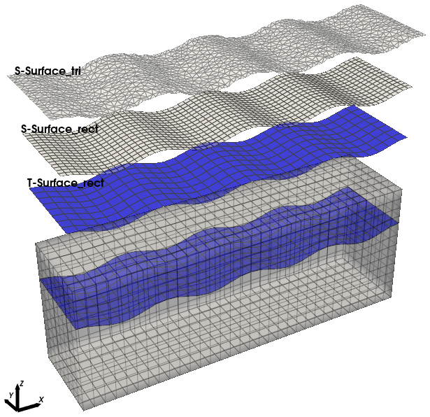
Figure 1 Illustration of the various objects and grids employed by the numerical model: the T-surface (in blue) represents the internal boundary of the Finite Element (FE) grid from tectonic modelling, while the S-surface corresponds to the surface from Badlands (triangle and rectangular mesh), modified from Thieulot et al. (2014).

For each tectonic time step, the Stokes equations are solved to obtain the velocity field across the entire domain by Underworld 2. The velocity on the S-surface is evaluated from the velocity field in Underworld 2 using the cubic spline method, and then transferred to Badlands, where the S-surface is further advected by solving the surface processes equation (with the evaluated velocity representing the uplift rate). Subsequently, the S-surface elevation is interpolated onto the T-surface, which is then remeshed accordingly. Particles are further adjusted based on changes in the T-surface by updating material indices, distinguishing between sediment and air (see Fig. 2a). More details about the remeshing algorithm within the ALE-IB scheme applied to free surface simulations can be found in Lu et al. (2026).

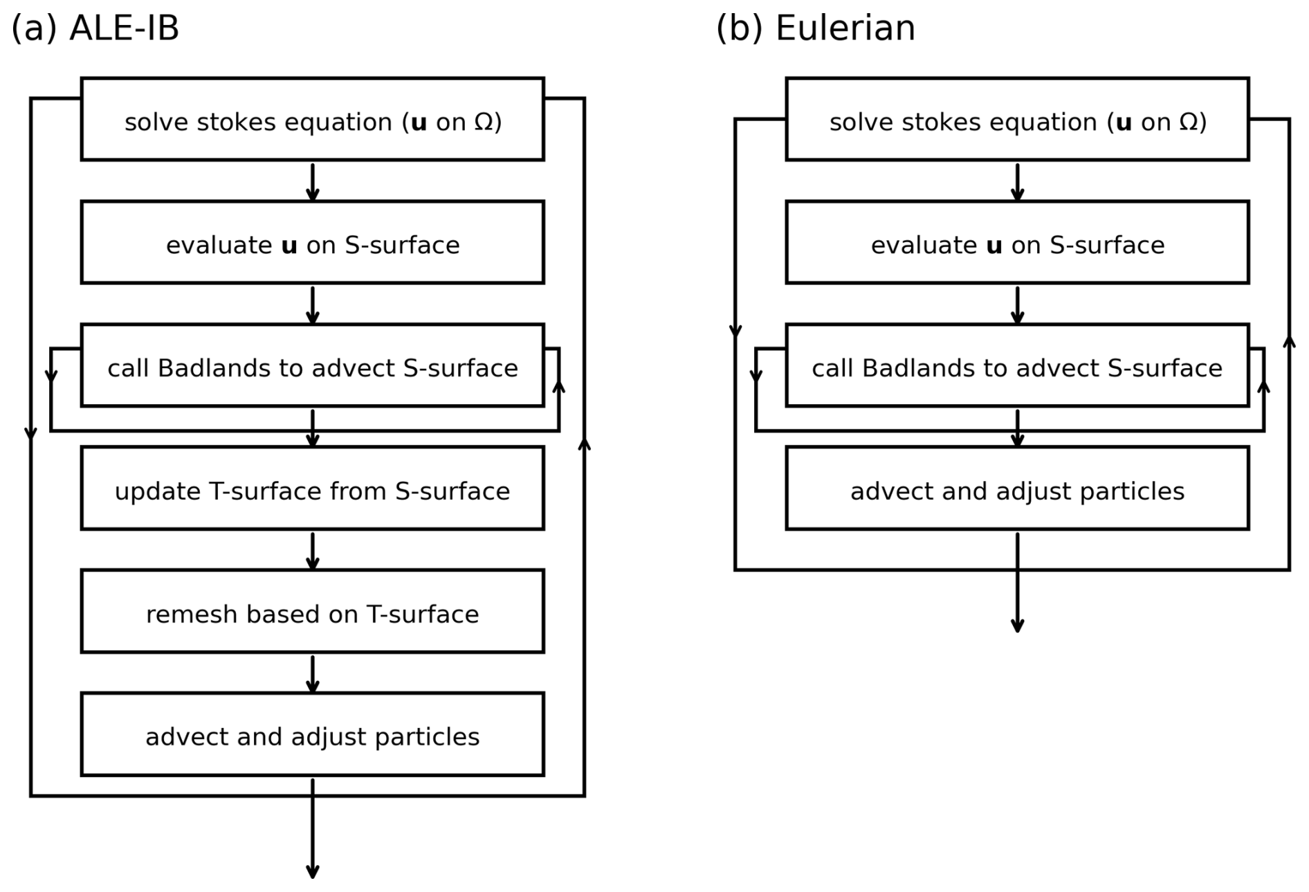
Figure 2 Flowchart presenting the coupling algorithm, (a) coupling within ALEI-IB scheme, (b) coupling within Eulerian scheme, modified from Thieulot et al. (2014).

2.2.2 Coupling within Eulerian scheme

The coupling modelling framework within the Eulerian scheme is implemented in the UWGeodynamics module (Beucher et al., 2019). We use this module to build models that investigate the interactions and feedback mechanisms between tectonic processes which primarily governed by lithospheric rheology, and surface processes responsible for material erosion and deposition. This module integrates the geodynamic code Underworld 2 (Moresi et al., 2007; Mansour et al., 2020) with surface process codes such as Badlands (Salles, 2016; Salles and Hardiman, 2016; Salles et al., 2018). UWGeodynamics is inspired by the Lithospheric Modelling Recipe (LMR) (Mondy, 2019), available on GitHub: https://github.com/LukeMondy/lithospheric_modelling_recipe (last access: 30 March 2026), originally developed for Underworld 1 (Moresi et al., 2002, 2003). The LMR, built on Underworld 1.8, facilitates model customization by providing easy access to boundary conditions, a library of rheologies, and modules for processes such as partial melting and surface processes (Mondy, 2019).

The coupled modelling framework provided by UWGeodynamics features a two-way, thermo-mechanical coupling that incorporates surface processes. Here, the velocity on the S-surface rectangle is derived from velocity field in Underworld 2 using the cubic spline method, and further advects the S-surface within the surface process model. As erosion and deposition alter the S-surface, the distribution of surface materials is dynamically updated (see Fig. 2b). The free surface simulation employs the “sticky air” method within the Particle-In-Cell Finite Element Method (PIC-FEM), utilizing an Eulerian scheme. In this approach, the surface is tracked by particles, and the “surface velocity” is interpolated from the mesh node velocities. In Badlands, the surface processes model typically requires smaller time intervals than the tectonic model. Therefore, the tectonic time step dt_tec is divided into multiple subtimesteps dt_sp to accommodate the surface processes model.

2.3 Model Setup

We have built two sets of experiments to investigate the evolution of lithosphere deformation and topography through fully coupled modelling. The first set couples the topography relaxation model with surface processes. The second set is based on the continental collision model modified from Vogt et al. (2018) and Knight et al. (2021). We compare models with and without surface processes, both in the Eulerian and ALE-IB schemes, and examine the difference between these two schemes. We also investigate the effect and sensitivity of LEM parameters. Model geometries and initial conditions for each set-up are shown in Fig. 3 and given in Tables 1, 2.

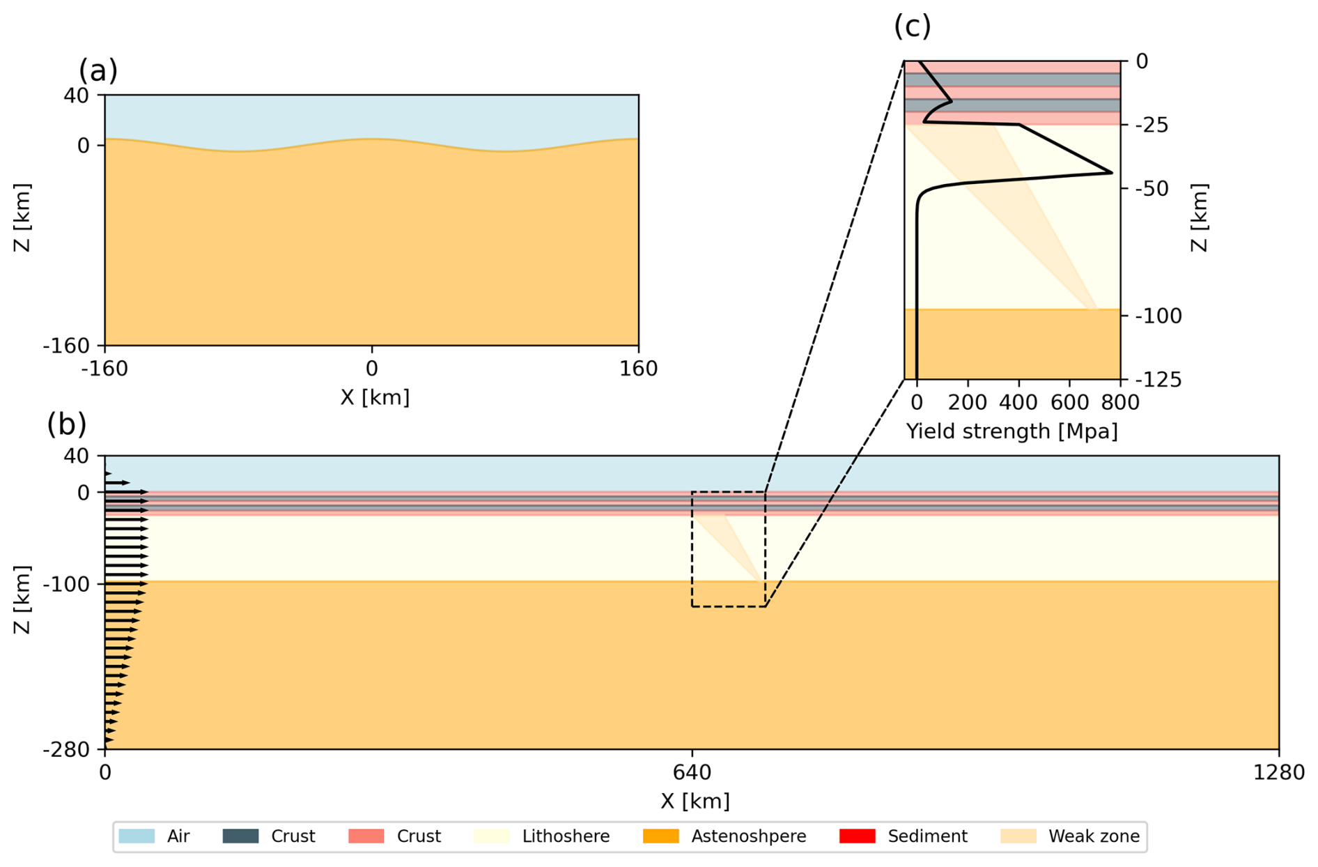
Figure 3 Model setup for (a) viscous relaxation of sinusoidal topography, (b) continental collision, (c) strength profile for the models of continental collision.

Table 1 Set of model tests with a series of parameters and simulation schemes: k_f the fluvial erosion coefficient, k_d the hillslope diffusion coefficient.

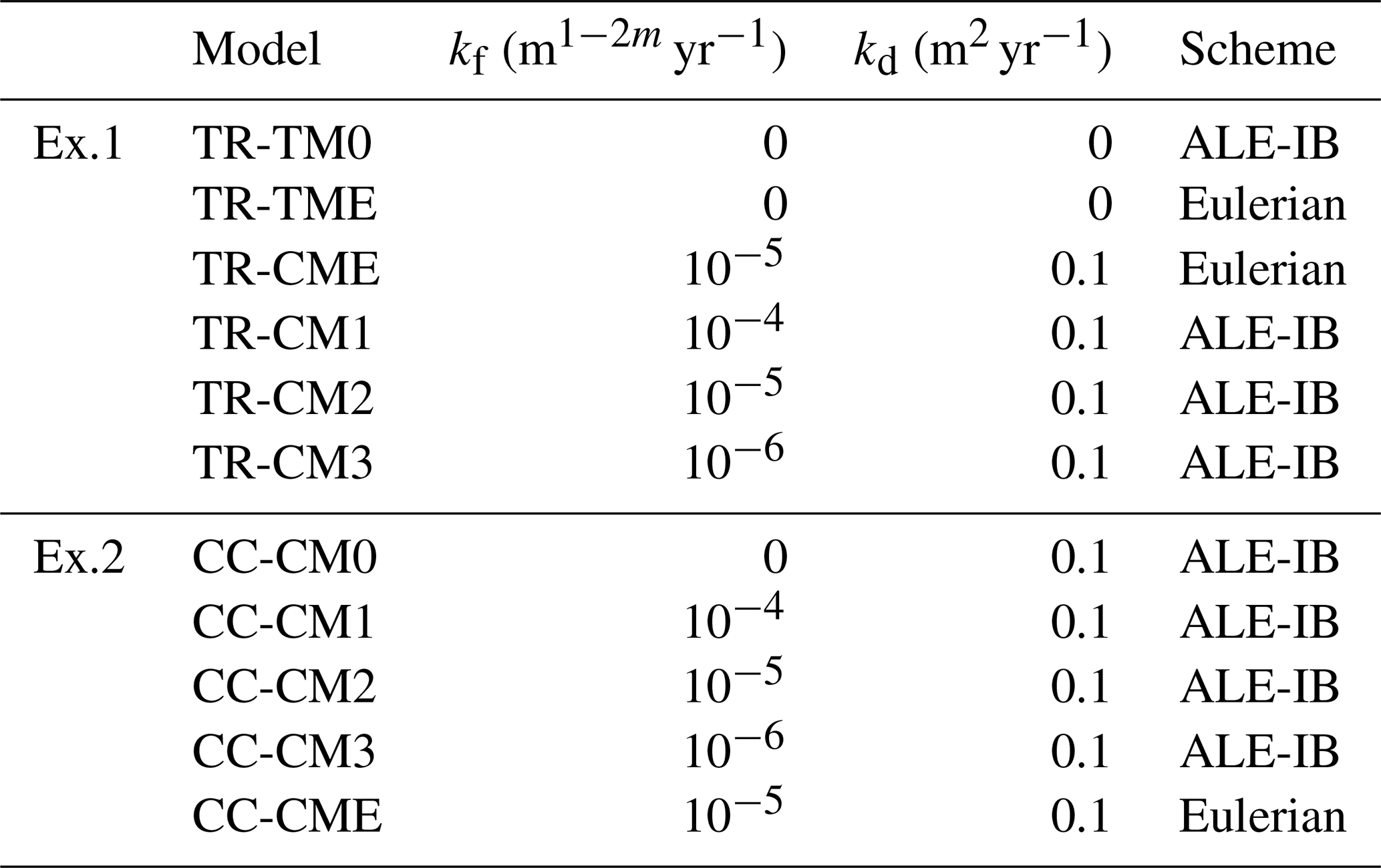
Notes: TR is short for topography relaxation, CC is short for continental collision, CM is short for coupling model, TM is short for tectonic model, E denotes Eulerian.

Table 2 Material properties.

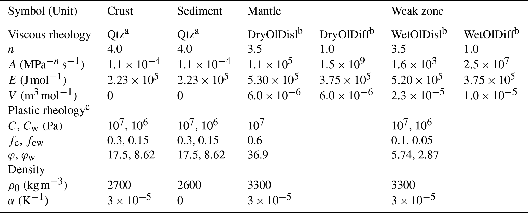
Notes: ρ₀ is the reference density, A is the preexponential factor, n is the stress exponent, V is the activation volume, E is the activation energy, f_c is the friction coefficient, φ is the internal friction angle, C is the cohesion at the surface. Subscript w represents the weakened value. Qtz is short for Quartzite, Ol is short for Olivine, Disl and Diff is short for Dislocation and Diffusion. ^a Gleason and Tullis (1995), ^bHirth and Kohlstedf (2003),^c Knight et al. (2021).

2.3.1 Topography relaxation

The loading of the Earth's surface can be described as the initial periodic surface displacement of an isoviscous fluid within an infinite half-space (Turcotte and Schubert, 2002). The setup is shown in Fig. 3a. The initial free surface displacement is given by:

$$\begin{array}{}\text{(12)}& {\displaystyle }{\displaystyle }w(x,\mathrm{0})=w_{\mathrm{0}}\cos \left(kx\right),\end{array}$$

where w₀=10 km is the initial load amplitude, $k=\mathrm{2}\mathit{\pi }/\mathit{\lambda }$ is the wave number, with λ=D (the wavelength). D=500 km is the depth of the model domain.

The analytical solution for the decay of topography is characterized by the relaxation time t^* (Zhong et al., 1996; Kramer et al., 2012):

$$\begin{array}{}\text{(13)}& {\displaystyle }{\displaystyle }w(x,t)=w(x,\mathrm{0}){\mathrm{e}}^{-t/t^{*}},\end{array}$$

with the relaxation time t^*:

$$\begin{array}{}\text{(14)}& {\displaystyle }{\displaystyle }{t}^{*}={\displaystyle \frac{Dk+\sinh \left(Dk\right)\cosh \left(Dk\right)}{{\sinh }^{\mathrm{2}}\left(Dk\right)}}{t}_{\mathrm{0}}^{*},t_{\mathrm{0}}^{*}={\displaystyle \frac{\mathrm{2}k\mathit{\eta }}{\mathit{\rho }g}},\end{array}$$

where η is the viscosity, ρ is the density. When λ≪D, $t^{*}\approx t_{\mathrm{0}}^{*}$.

The computational domain is 320 km×200 km for the ALE-IB and Eulerian schemes. A constant time step of 2.5 ka was employed here, using Q₁dQ₀ finite elements and a mesh of 129×81 nodes, with 16 particles per cell. Material properties are: $\mathit{\rho }=\mathrm{3300}\mathrm{kg}{\mathrm{m}}^{-\mathrm{3}}$ and η=10²¹ Pa s for the lithosphere layer, $\mathit{\rho }=\mathrm{0}\mathrm{kg}{\mathrm{m}}^{-\mathrm{3}}$ and η=10¹⁸ Pa s for the air layer, $\mathit{\rho }=\mathrm{2700}\mathrm{kg}{\mathrm{m}}^{-\mathrm{3}}$ and η=10¹⁹ Pa s for the sediment layer. Gravitational acceleration is $g=\mathrm{9.81}\mathrm{m}{\mathrm{s}}^{-\mathrm{2}}$. The side boundaries are free-slip, the bottom is no-slip, and the top boundary is free-slip over sticky air.

2.3.2 Continental collision

The second experimental set couples a 2D thermo-mechanical model with surface processes to study the integrated influence of tectonics and surface processes on continental collision. The setup is shown in Fig. 3b and c. The tectonic models part is adapted from Vogt et al. (2018) and Knight et al. (2021). In their work, they discuss how convergence rate, crustal thickness, and rate-dependent viscous rheology control the strength of the wedge and the resulting structural style.

The computational domain measures 1280 km×320 km for both the ALE-IB and Eulerian schemes, discretized with Q₁dQ₀ finite elements on a 513×129 node grid, with 30 particles per cell. The initial configuration consists of a homogeneous crust with a 45° dipping weak zone within the mantle lithosphere at x=640 km, representing a pre-existing subduction zone. The crust is 25 km thick and is overlain by a 40 km-thick sticky-air layer. Tectonic and surface-process time steps are 10 and 5 ka, respectively.

A constant surface temperature of T=0 °C (and for air material) is imposed, and the side boundaries are adiabatic (no heat flux). The initial temperature distribution follows a geotherm: 25 °C km⁻¹ from surface down to 10 km depth, then 12 °C km⁻¹ to the lithosphere–asthenosphere boundary (LAB) at a depth of 97.5 km, where T=1300 °C. The velocity boundaries are configured as follows: free-slip conditions are applied on the right and top boundaries; the bottom boundary is unconstrained to allow inflow/outflow, effectively placing the model above an infinite space with an inviscid fluid at a depth of 280 km (Gerya, 2009). Convergence is imposed at the left boundary with a fixed velocity of 5 cm yr⁻¹, applied throughout the crust and mantle lithosphere. Below the lithosphere, the velocity decreases linearly from the convergence value at the base of the lithosphere to zero at the bottom boundary. Above the crust, an inflow/outflow is prescribed across the sticky-air layer to permit surface topography development.

2.3.3 Surface Processes Parameters

The surface processes considered include hillslope and fluvial processes. The hillslope process is modeled using the linear diffusion equation as shown in Eq. (11). In this study, the diffusion coefficient is set as a constant $k_{\mathrm{d}}=\mathrm{0.1}{\mathrm{m}}^{\mathrm{2}}{\mathrm{yr}}^{-\mathrm{1}}$ (Salles, 2016). Typically, diffusion coefficients range from 0.001 to 10 (Roering et al., 1999) in various environments, but the model evolution usually is not sensitive to variations in hillslope parameters (Ueda et al., 2015). For our simulations, we use a relatively high, realistic value across aerial, marine, and river settings to produce smoother topography. This helps to prevent excessive surface distortion and simplifies the landscape modelling.

The fluvial process is modeled using the stream power law equation as shown in Eq. (10), with landscape evolution simulated under a uniform rainfall rate of 1 m yr⁻¹. The fluvial erodibility coefficient k_f exhibits significant uncertainty and spans a wide range, as it depends on various factors, including climate, rock type, channel width, hydraulics, and others (Stock and Montgomery, 1999; Dietrich et al., 2003). In this study, k_f is assumed to be spatially uniform across the entire region. For sensitivity analysis, we explore a range of values from 10⁻⁴ to ${\mathrm{10}}^{-\mathrm{6}}{\mathrm{m}}^{\mathrm{1}-\mathrm{2}m}{\mathrm{yr}}^{-\mathrm{1}}$. The exponents m and n are set to 0.5 and 1, respectively, based on the unit stream power model (Whipple and Tucker, 1999). Alternative values for m and n can be found in Gasparini and Brandon (2011).

3 Results and discussion

3.1 Topography relaxation

3.1.1 Models with and without surface processes in ALE-IB and Eulerian schemes

In the models without the surface processes from Experiment 1, the relaxation of an initial topography toward equilibrium occurs over approximately 300 ka. Figure 4a and b compare the topography results obtained from free-surface simulations conducted with and without surface processes (where $k_{\mathrm{d}}=\mathrm{0.1}{\mathrm{m}}^{\mathrm{1}-\mathrm{2}m}{\mathrm{yr}}^{-\mathrm{1}}$, $k_{\mathrm{f}}={\mathrm{10}}^{-\mathrm{4}}{\mathrm{m}}^{\mathrm{1}-\mathrm{2}m}{\mathrm{yr}}^{-\mathrm{1}}$) across two different numerical schemes: ALE-IB and Eulerian at Time=150 ka (approximately 2τ^*). The results from the models without surface processes (TR-TM and TR-TME) demonstrate that the simulation employing the ALE-IB scheme exhibits excellent agreement with the analytical solution, highlighting its accuracy in capturing topographic features. Conversely, the Eulerian scheme displays fluctuations that diminish the overall accuracy. The L₂-norm error between the ALE-IB scheme and the analytical solution is 0.00040, while the error for the Eulerian scheme is 0.00113.

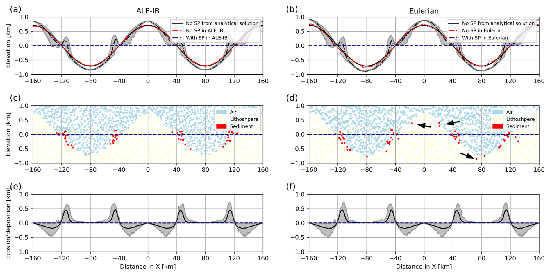
Figure 4 Topography, erosion and deposition of the relaxation model in ALE-IB and Eulerian scheme at Time=0.15 Ma, the dark blue line indicates the sea level. (a, b) Topography: the grey shaded area shows the range between the maximum and minimum topography values produced by the model with surface processes (SP), while the black line represents the average topography. (c, d) Material field: distribution of material properties within the model, the arrows indicate particle fluctuations. (e, f) Erosion and deposition: quantification of surface processes over time, showing accumulated erosion and deposition. The grey shaded area denotes the range between maximum and minimum values, and the black line represents the average value.

As illustrated in Fig. 4e and f, in coupling models, erosion predominantly accumulates in the mid-section of the hill above sea level, driven by fluvial erosion processes which positively correlated with slope. Sediment deposition, on the other hand, tends to occur near sea level. The relative difference in the average depth of erosion and deposition between these two schemes is 24.7 %.

The superior performance of the ALE-IB scheme can be attributed to its more precise velocity estimation and the ability to track topographic changes more accurately. Consequently, sediment transport and distribution are represented more realistically, as shown in Fig. 4c. In contrast, the Eulerian scheme results in some nonphysical sediment accumulation along the downhill slope below sea level, shown in Fig. 4d, likely due to less accurate velocity interpolation and topography tracking.

3.1.2 Coupling models with varying fluvial parameters in the ALE-IB Scheme

Raising the fluvial erodibility coefficient substantially enhances incision and sediment transport. By 150 ka, landscapes with higher k_f exhibit deeper valley incision and a more convex longitudinal profile, consistent with increased valley widening and stronger hillslope–channel coupling (Fig. 5). A small topographic peak forms near sea level at the hills' toe, likely reflecting a transient balance between base-level lowering and localized deposition. The drainage network becomes more expansive as channel incision intensifies (Fig. 5g). Across the 10–300 ka time series (Fig. 6), the elevated-erodibility regime yields larger changes in relief and in channel geometry, indicating that fluvial processes dominate landscape evolution under stronger erodibility.

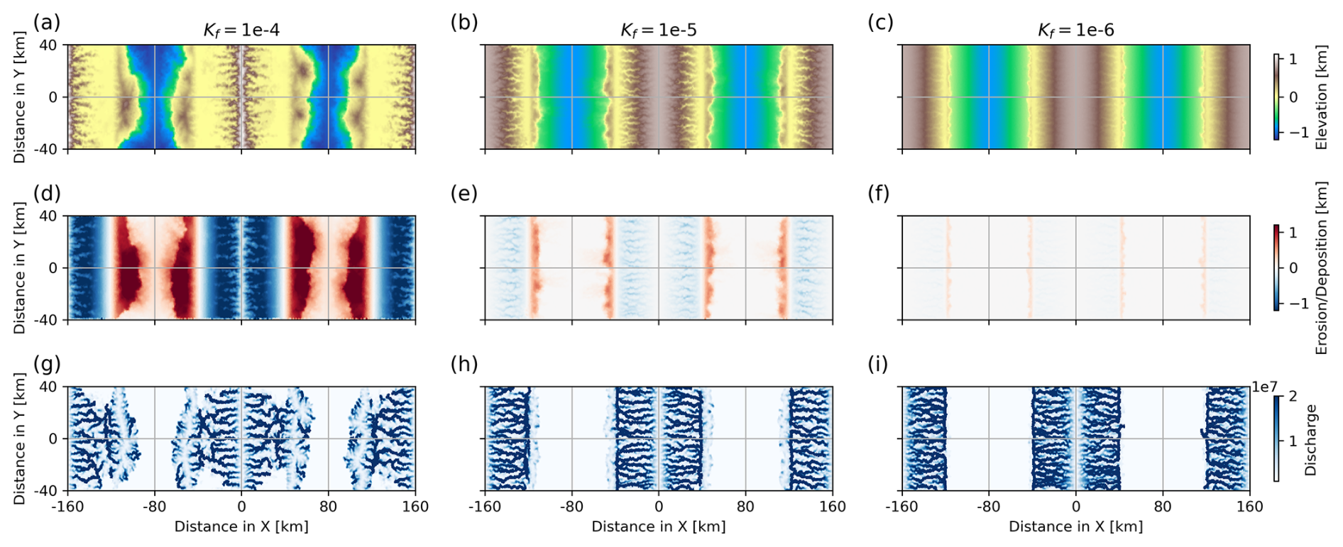
Figure 5 Comparison of models in Experiment 1 with different fluvial erosion parameters at Time=0.15 Ma. (a–c) Topography; (d–f) erosion and deposition; (g–i) river system.

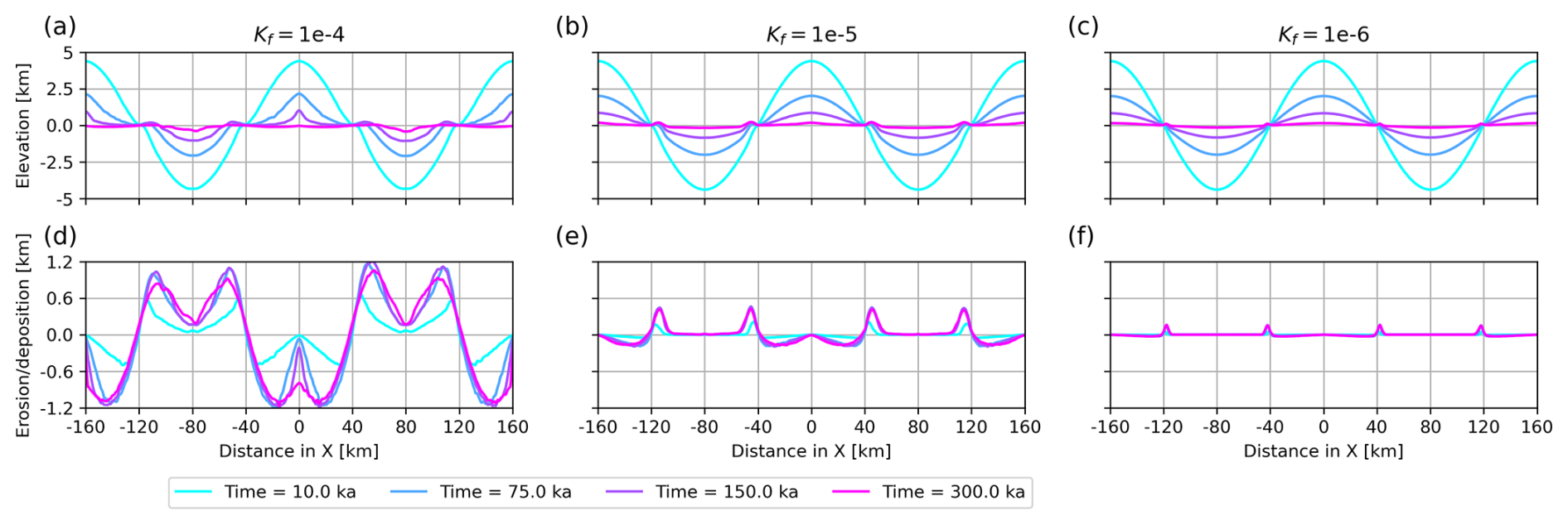
Figure 6 Comparison of the temporal evolution of models in Experiment 1 with varying fluvial erosion parameters. (a–c) Topography; (d–f) erosion and deposition.

3.2 Continental collision

Model CC-CM0 from Experiment 2 (Fig. 7) employs the coupling framework within the ALE-IB scheme. As it couples only with the hillslope diffusion process, the model evolves with minimal sediment accumulation. Deformation localizes above the lithospheric weak zone, forming conjugate shear zones that propagate outward over time. This results in progressive crustal stacking, evident from the localized bands of high strain. The stacking is accommodated between the shear zones, ultimately developing into a thick, narrow wedge.

Figure 7 Evolution of material and plastic strain field in CC-CM0 from Experiment 2 through time. (a–c) Material; (d–f) Plastic strain.

3.2.1 Coupling models in ALE-IB and Eulerian schemes

Models CC-CM2 and CC-CME employ the coupling framework within the Arbitrary Lagrangian–Eulerian Immersed Boundary (ALE-IB) and Eulerian schemes separately, with identical settings for tectonic and surface processes. The deformation evolution in the crust and lithosphere resembles that of Model CC-CM0, but features a narrow shear zone in the middle of the wedge due to sedimentation accumulating on both sides of the wedge (Figs. 7, 8, and 9). This sedimentation mass enhances wedge uplift, ultimately forming a narrower and higher wedge. This outcome aligns with the perspective in Avouac and Burov (1996) that erosion can drive the growth of intracontinental mountains.

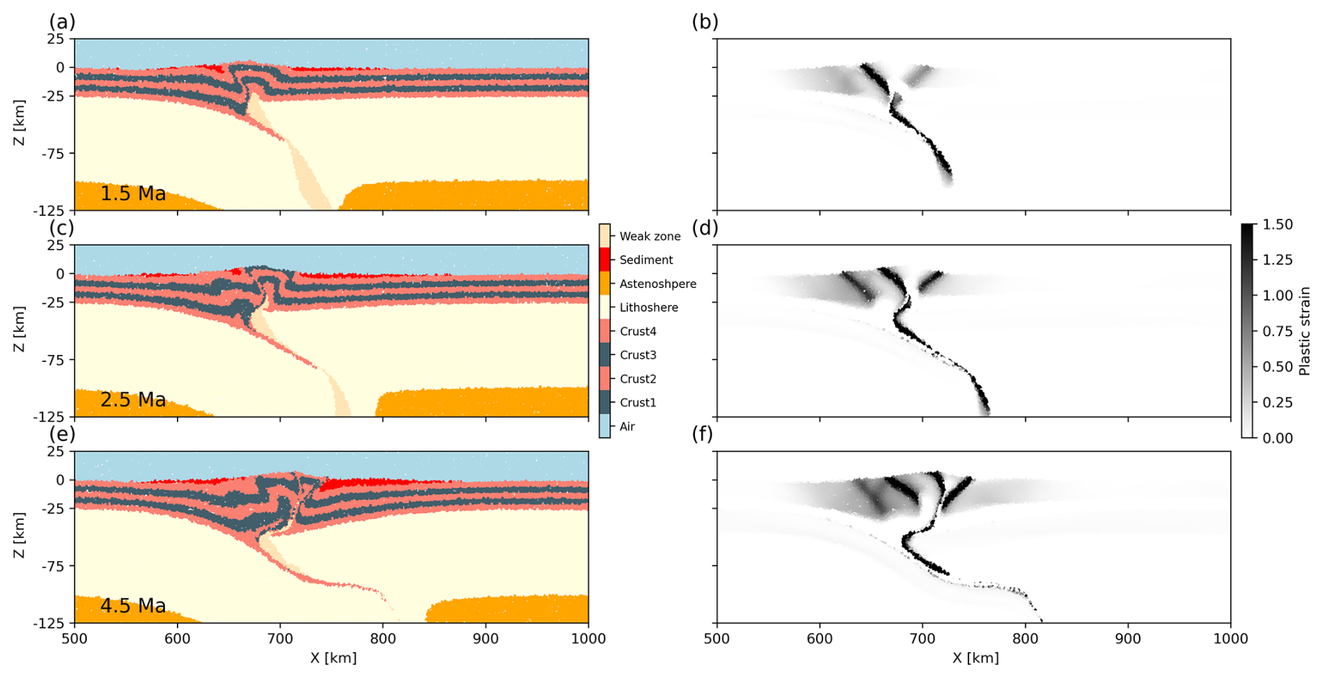
Figure 8 Evolution of material and plastic strain field in CC-CM2 from Experiment 2 through time. (a–c) Material; (d–f) Plastic strain.

Figure 9 Evolution of material and plastic strain field in CC-CME from Experiment 2 through time. (a–c) Material; (d–f) Plastic strain.

The deformation patterns do not differ substantially between the ALE-IB and Eulerian schemes (Fig. 10), though differences emerge in the late stage viscosity field due to slight variations in strain rate, stemming from minor differences in sediment distribution. The ALE-IB scheme shows more sedimentation in the upper plate and less in the lower plate compared to the Eulerian scheme (Figs. 10c and d, 11c and d). The Eulerian scheme exhibits fluctuations that reduce overall accuracy, as evidenced by sediment distributions far from the wedge. On the left side of the sediments in the lower plate, small topographic peaks appear in the material field but are absent from the river patterns in the results from the Eulerian scheme (Fig. 11f). The relative difference in the average depth of erosion and deposition between these two schemes is 93.3 %. These discrepancies may arise from inaccurate velocity evaluations and surface tracing. Topographic gradients exhibit local changes in high-strain areas, which clearly link to river system patterns: rivers evolve along the sides of small peaks or become diverted in these regions, as prominently shown in the ALE-IB scheme results (Fig. 12e).

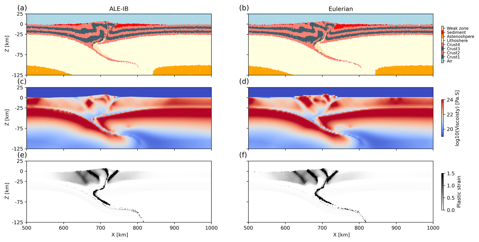
Figure 10 (a, b) Material, (c, d) viscosity, and (e, f) accumulated plastic strain of the coupling model in ALE-IB and Eulerian scheme (CC-CM2 and CC-CME) at Time=4.5 Ma.

3.2.2 Coupling models with varying fluvial parameters in the ALE-IB Scheme

Models CC-CM1 and CC-CM3 employ the coupling framework within the Arbitrary Lagrangian–Eulerian Immersed Boundary (ALE-IB) scheme, with varying fluvial erosion parameters. In Model CC-CM3, the deformation evolution (Fig. 14) closely resembles that of CM0, owing to the relatively low fluvial erosion parameters, which result in subdued surface processes and preserved crustal thickening. In contrast, Model CM1 exhibits markedly different crustal deformation due to intense erosion and deposition driven by high fluvial erosion parameters. This strong erosional regime disrupts the typical crustal stacking patterns, yielding a thin, wide wedge with low topography and relief, characterized by two localized bands of high strain (Fig. 13).

Rather than forming multiple mountain ranges, as seen in models with weaker erosion, CC-CM1 develops only a single prominent mountain peak (Fig. 16a and b), accompanied by simpler river patterns (Fig. 17e and f). This outcome highlights how enhanced fluvial incision can promote efficient mass removal from the orogen, leading to isostatic rebound and lateral spreading of the wedge, consistent with critical taper theory where erosion reduces the wedge's taper angle and stabilizes a broader, lower-relief structure (Ueda et al., 2015). For instance, similar dynamics are observed in natural settings, such as the eastern Tibetan Plateau margins, where high erosion rates flatten topography and simplify drainage networks (Kirby and Ouimet, 2011). These variations highlight the sensitivity of coupling models to surface process parameters: in high-erosion scenarios, such as CC-CM1, fluvial systems act as a feedback mechanism, channelling sediment transport and influencing lithospheric strain localization.

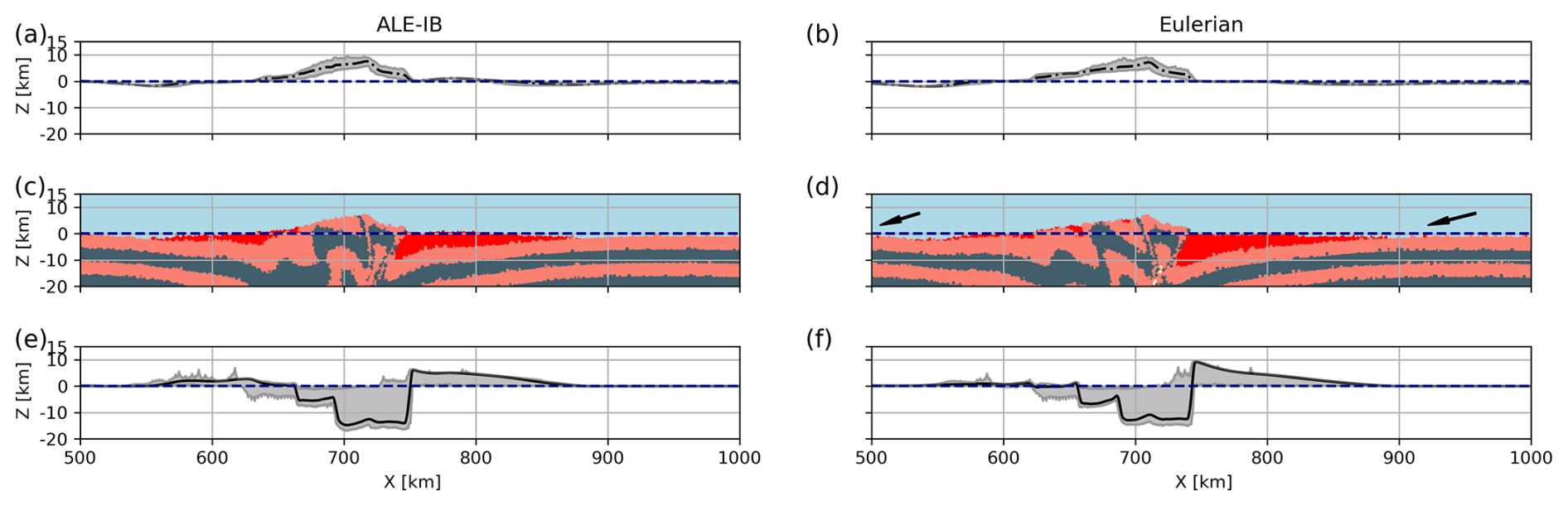
Figure 11 Topography, erosion and deposition at Time=4.5 Ma of the coupling model in ALE-IB and Eulerian scheme (CC-CM2 and CC-CME), the dark blue line indicates the sea level. (a, b) Topography: the grey shaded area shows the range between the maximum and minimum topography values, while the black line represents the average topography. (c, d) Material field: distribution of material properties within the model, the arrows indicate particle fluctuations. (e, f) Erosion and deposition: quantification of surface processes over time, showing accumulated erosion and deposition. The grey shaded area denotes the range between maximum and minimum values, and the black line represents the average value.

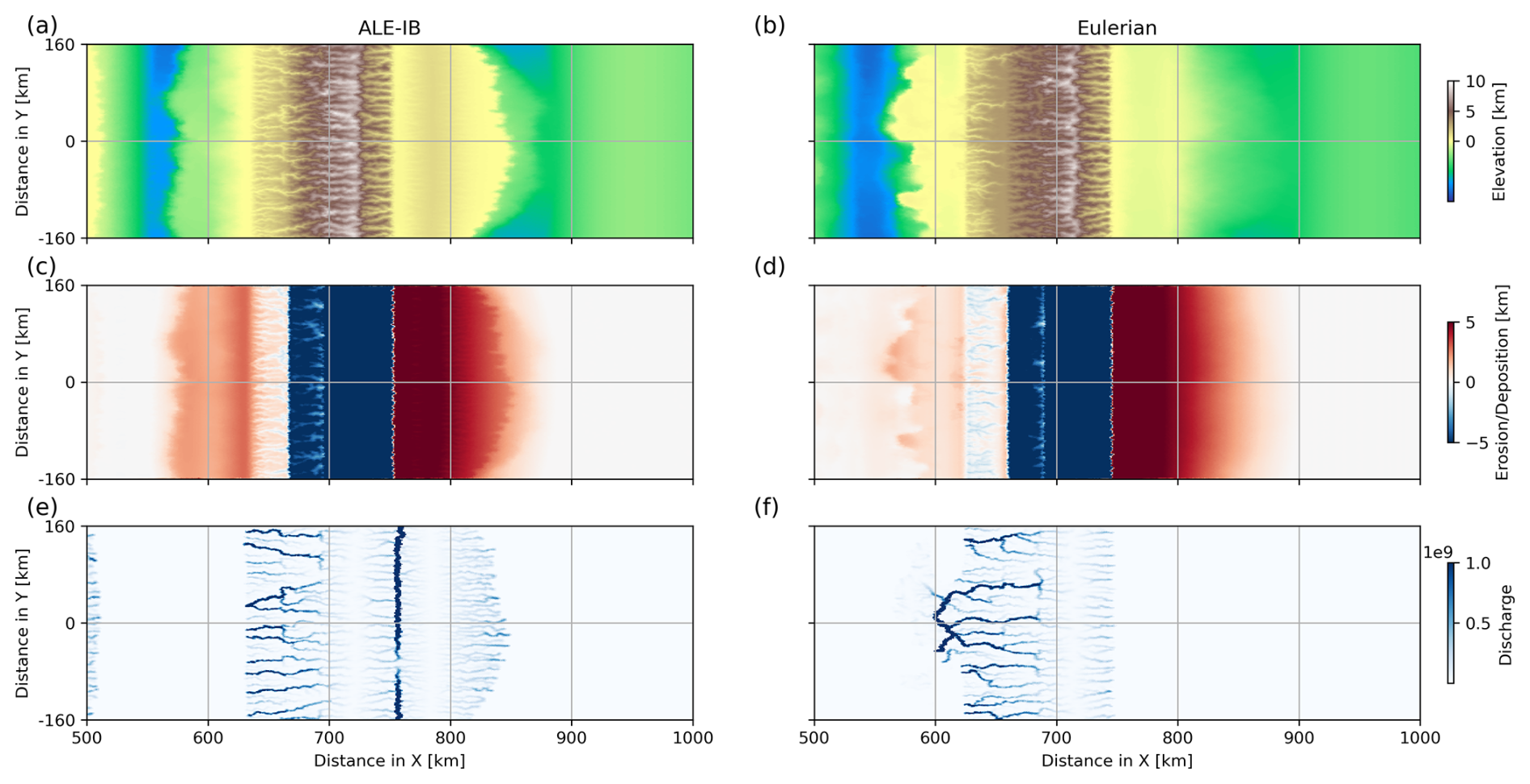
Figure 12 CC-CM2 and CC-CME at Time=4.5 Ma. (a–c) Topography; (d–f) erosion and deposition; (g–i) river system.

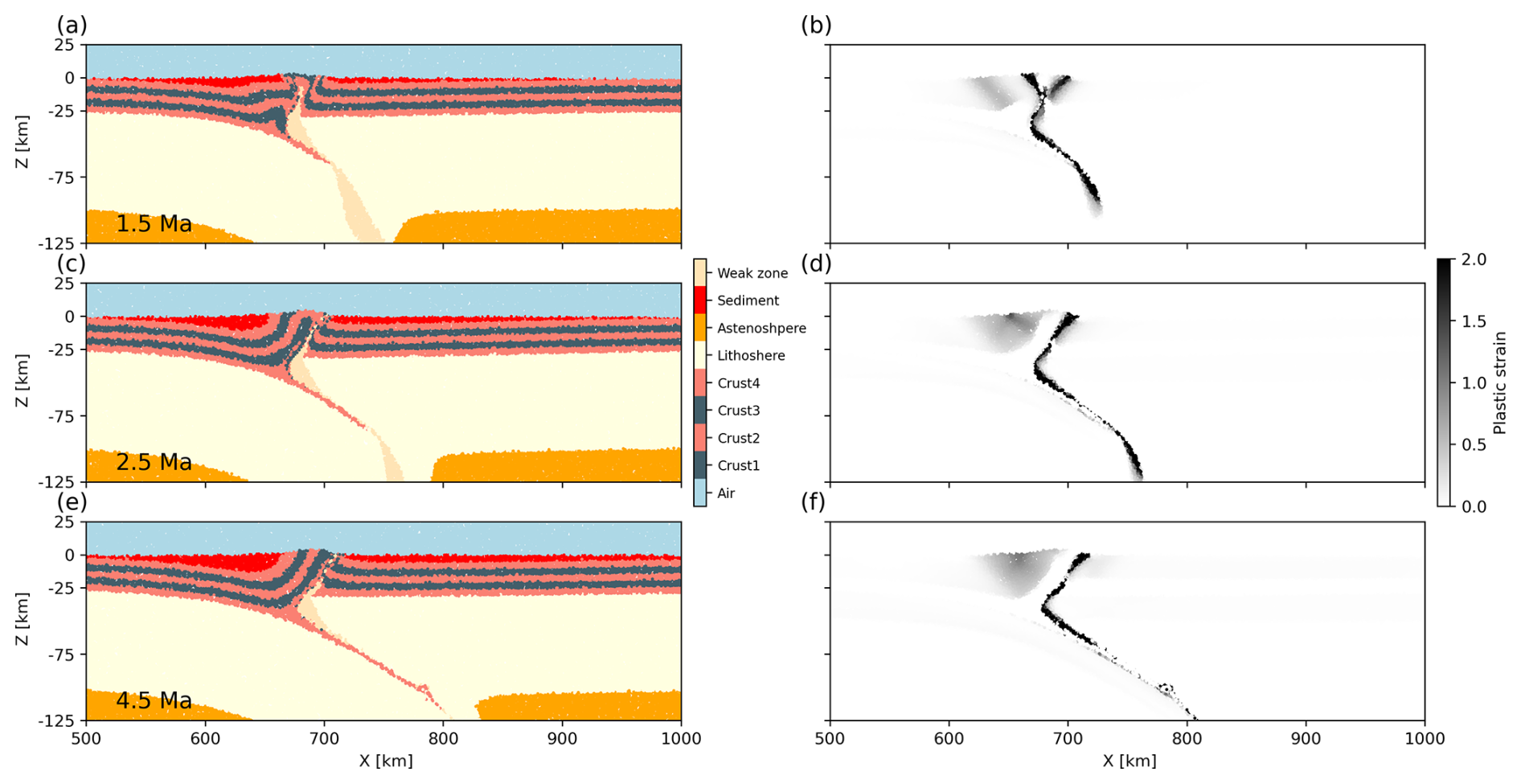
Figure 13 Evolution of material and plastic strain field in CC-CM1 from Experiment 2 through time. (a–c) Material; (d–f) Plastic strain.

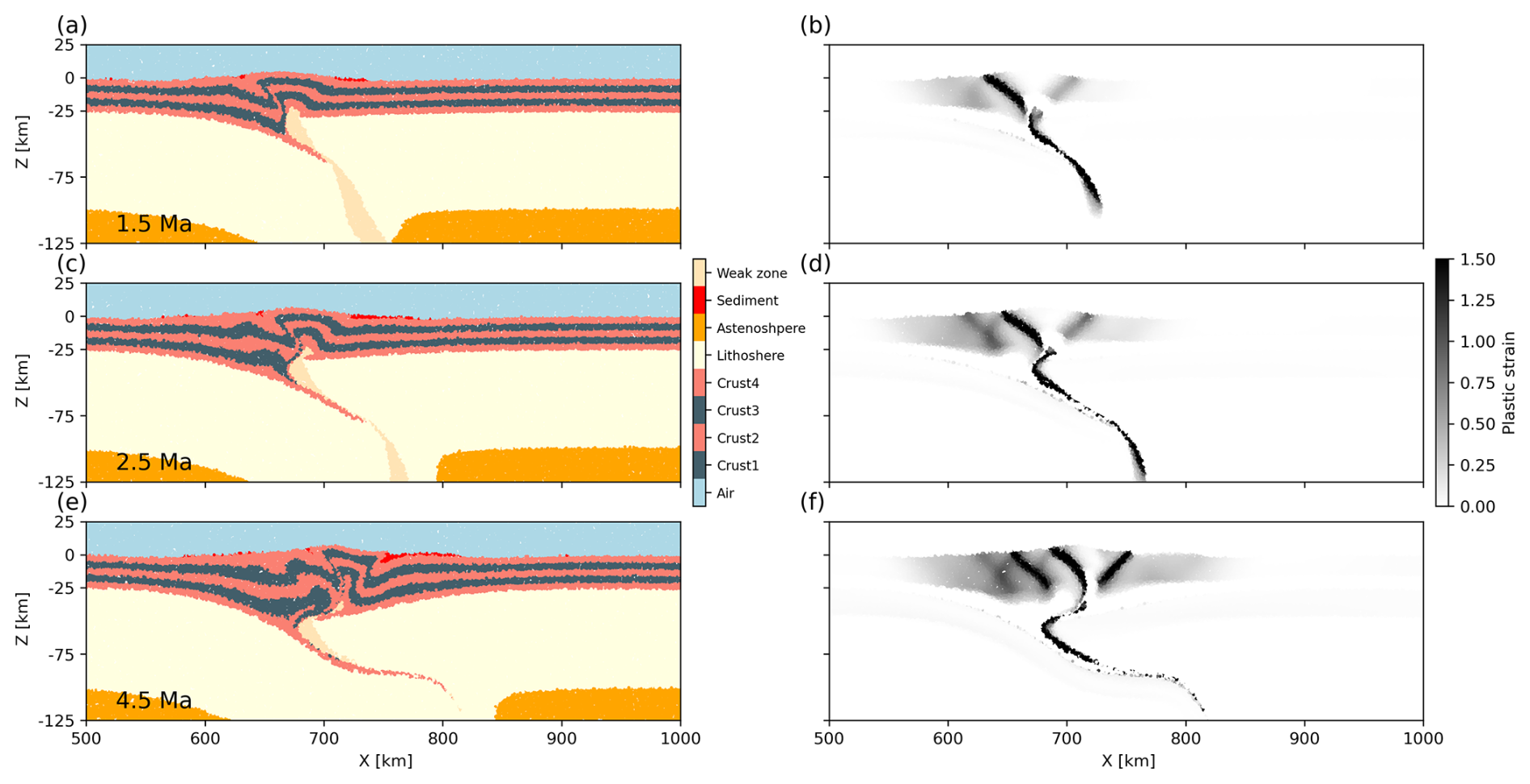
Figure 14 Evolution of material and plastic strain field in CC-CM3 from Experiment 2 through time. (a–c) Material; (d–f) Plastic strain.

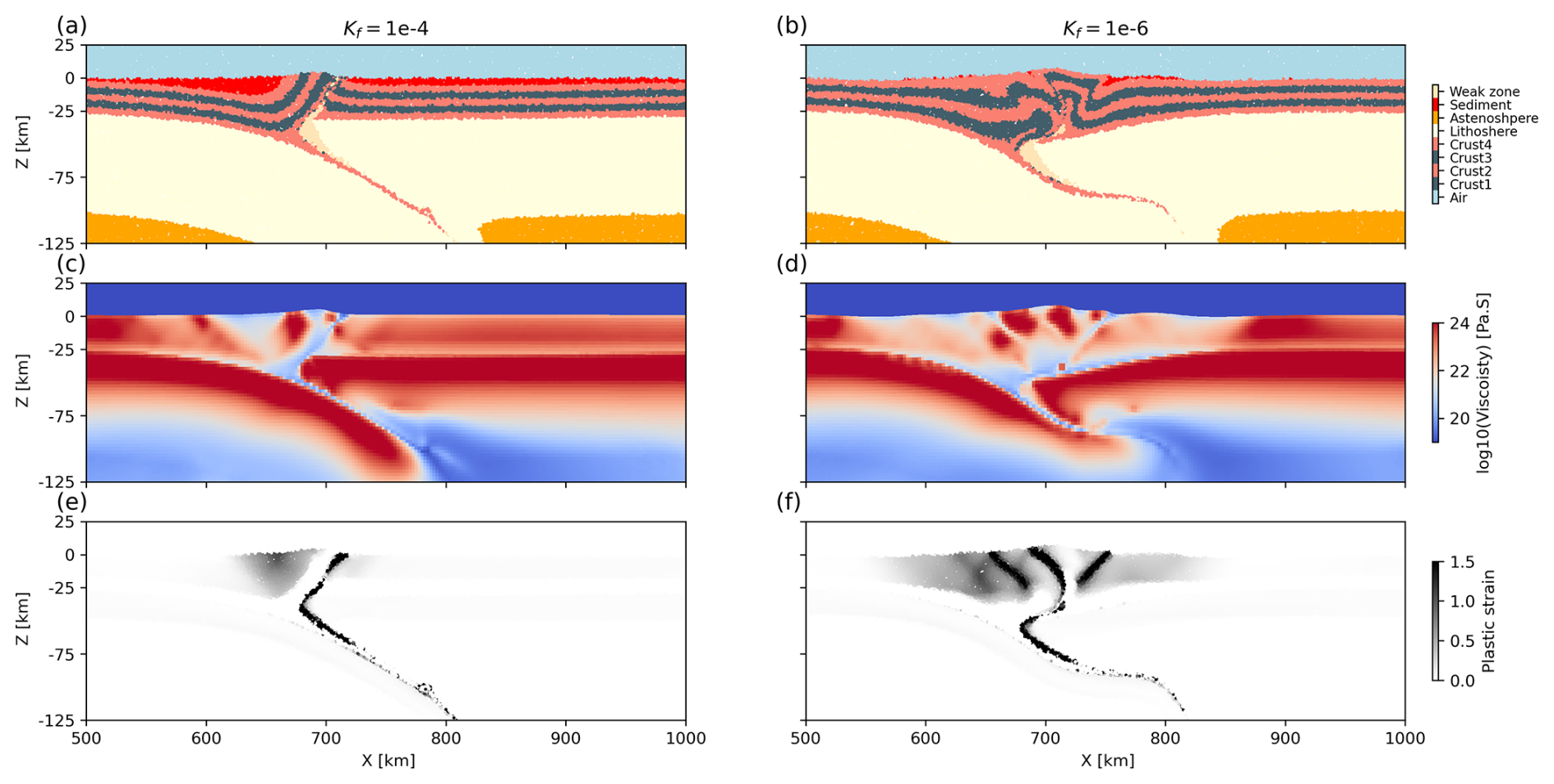
Figure 15 (a, b) Material, (c, d) viscosity, and (e, f) accumulated plastic strain of the coupling model in ALE-IB scheme with different fluvial erosion parameters (CC-CM1 and CC-CM3) at Time=4.5 Ma.

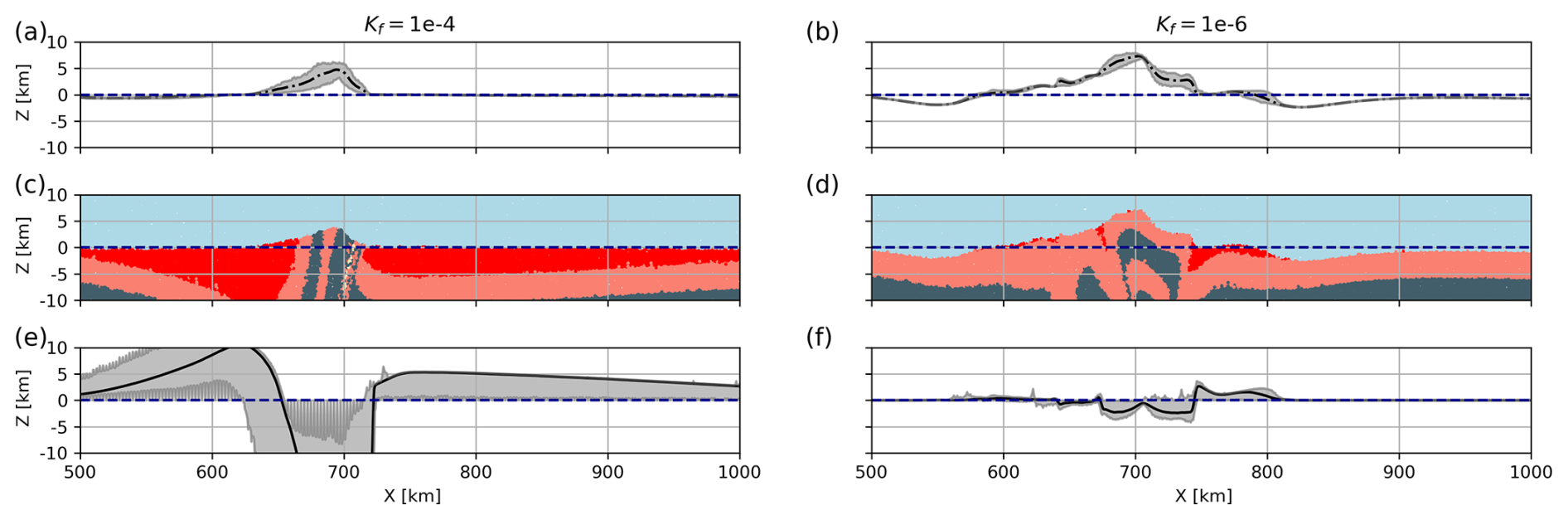
Figure 16 Topography, erosion and deposition of the coupling model in ALE-IB scheme (CC-CM1 and CC-CM3) at Time=4.5 Ma, the dark blue line indicates the sea level. (a, b) Topography: the grey shaded area shows the range between the maximum and minimum topography values, while the black line represents the average topography. (c, d) Material field: distribution of material properties within the model, the arrows indicate particle fluctuations. (e, f) Erosion and deposition: quantification of surface processes over time, showing accumulated erosion and deposition. The grey shaded area denotes the range between maximum and minimum values, and the black line represents the average value.

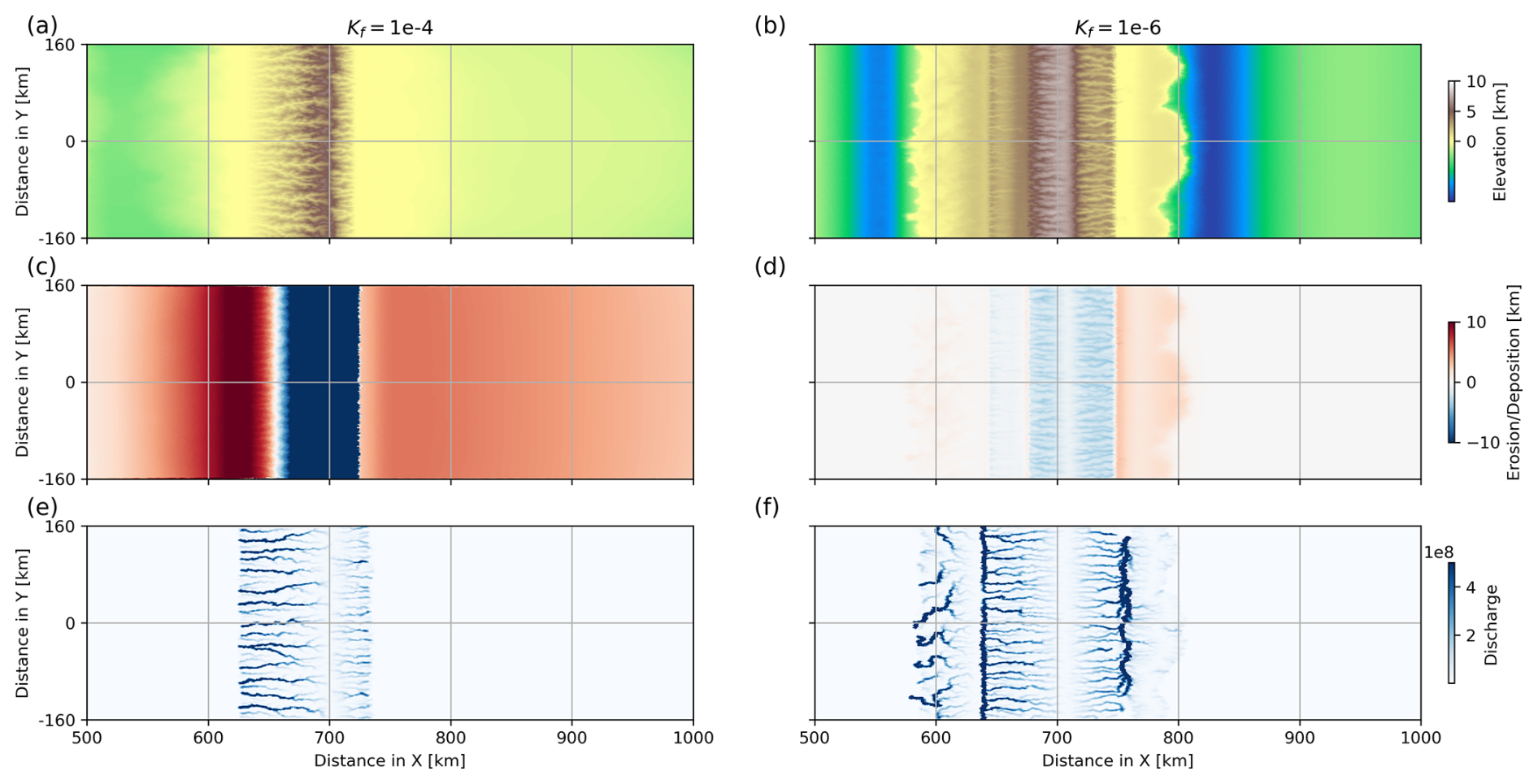
Figure 17 CC-CM1 and CC-CM3 at Time=4.5 Ma. (a–c) Topography; (d–f) erosion and deposition; (g–i) river system.

3.2.3 Model Limitations

Our models show the advantages of the ALE-IB coupling scheme over a purely Eulerian one, although no comparisons were made to a pure ALE implementation (Thieulot et al., 2014; May et al., 2014). The implementation of the ALE-IB method allows for straightforward handling of particles belonging to different materials (such as air, sediment and crust) across the free surface interface (the boundary between air and rock). There is no need to consider void spaces or other issues that arise when using the ALE scheme. This method is more efficient in the study of surface processes (e.g. erosion and sedimentation) because the interfaces between two phases are implicitly tracked and less numerical diffusion is present, as shown by Model CC-CM2 vs. Model CC-CME.

In nature, the evolution of orogenic wedges is inherently three-dimensional and involves a broad spectrum of complexities, including laterally and vertically varying rheological heterogeneities (e.g. due to compositional differences or thermal gradients) and structural inheritance (e.g. pre-existing faults or basement fabrics), all of which profoundly influence deformation patterns and topographic development. For instance, in real-world systems like the Himalayas or the Andes, these factors lead to asymmetric wedge growth, localized uplift, and complex drainage networks that cannot be fully captured in 2D simulations. Our model tests here remain limited to 2D due to the consideration of affordable computational costs, which restrict the resolution and scale of simulations. However, the ALE-IB coupling framework we propose is inherently scalable and supports 3D implementation. It leverages modern high-performance computing techniques, such as parallel processing and adaptive mesh refinement, both of which are capabilities of Underworld 2, to efficiently manage computational costs.

This framework's extensibility opens avenues for future research, including direct comparisons with the pure ALE scheme to quantify trade-offs in computational efficiency vs. accuracy, as well as 3D extensions of Models to explore erosion-driven feedback in more realistic geometries. Integrating field observations or geophysical data (e.g. seismic tomography for rheological constraints) could further help validate these models, enhancing their predictive power for understanding intracontinental orogeny and landscape evolution.

4 Conclusions

This study introduces a novel coupling framework that integrates the geodynamic codes Underworld 2 with the surface process model Badlands within the Arbitrary Lagrangian–Eulerian with Internal Boundary (ALE-IB) scheme. By addressing the limitations of traditional Eulerian-based approaches, this framework enables more accurate and efficient two-way interactions between tectonic deformation and surface processes, such as fluvial erosion, hillslope diffusion, and sedimentation. Our methodology leverages the finite element method with particle-in-cell techniques to solve conservation equations for momentum, mass, and heat, while incorporating visco-plastic rheologies, strain weakening, and power-law creep to simulate lithospheric behaviour. The integration with Badlands further accounts for mass continuity through fluvial and diffusive transport, providing a robust platform for exploring erosion-tectonic feedbacks.

Through systematic experiments, we demonstrate that the ALE-IB framework outperforms Eulerian schemes in handling free surfaces, material interfaces, and sediment distribution, leading to reduced numerical artifacts, improved velocity tracking, and more realistic topographic and river pattern evolution. For instance, models with varying fluvial parameters reveal how intense erosion disrupts crustal stacking, favouring thin, wide wedges with simplified drainage networks, while minimal erosion promotes thick, narrow wedges with localized strain – outcomes consistent with erosion-driven orogenic growth theories (Avouac and Burov, 1996). Comparisons highlight subtle differences in viscosity fields and sediment accumulation, underscoring ALE-IB's advantages in precision without excessive computational complexity.

These findings advance our understanding of coupled geodynamic systems, emphasizing the role of surface processes in modulating lithospheric deformation and landscape evolution. By bridging deep Earth dynamics with surface topography, the framework offers insights into natural orogens, such as the Himalayas or Tibetan Plateau, where rheological heterogeneities and erosion feedbacks shape long-term tectonics. However, our 2D simulations, necessitated by computational limits, inherently simplify the 3D complexities, such as lateral heterogeneity in structure and rheology.

Nevertheless, the proposed ALE-IB coupling framework is scalable to 3D implementations, paving the way for future benchmarking against pure ALE schemes, incorporation of stochastic elements in surface processes, and integration with observational data (e.g. seismic or geomorphic datasets). This would expand the scope of predictive models seeking to understand climate-tectonic feedbacks and possibly even establish some specific value ranges for tectonic wedges analysis. Ultimately, this work aims to facilitate the inevitable evolution of geodynamic modelling toward more holistic and accurate coupling simulations of Earth's dynamical surface and interior.

Appendix A

A1 Coupling models of experiment 1 with high fluvial parameter in ALE-IB and Eulerian schemes

Here we present the results from the experiment 1, the coupling models utilize high fluvial parameters, specifically with a fluvial erodibility coefficient of $k_{\mathrm{f}}={\mathrm{10}}^{-\mathrm{4}}{\mathrm{m}}^{\mathrm{1}-\mathrm{2}m}{\mathrm{yr}}^{-\mathrm{1}}$. Increasing the fluvial erodibility coefficient significantly enhances both incision and sediment transport, which is effective for both schemes. The hills exhibit a pronounced convex shape, and the models generate a substantial amount of sediment near and below sea level (see Fig. A1a–d). As illustrated in Fig. A1e and f, the relative difference in the average depth of erosion and deposition between these two schemes is 21.3 %. This suggests that the advantages of ALE-IB do not scale with increased levels of erosion and deposition.

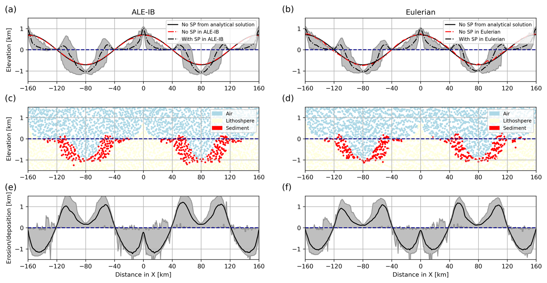
Figure A1 Topography, erosion and deposition of the relaxation model in ALE-IB and Eulerian scheme at Time=0.15 Ma, the dark blue line indicates the sea level. (a) and (b) Topography: the grey shaded area shows the range between the maximum and minimum topography values produced by the model with surface processes (SP), while the black line represents the average topography. (c) and (d) Material field: distribution of material properties within the model. (e) and (f) Erosion and deposition: quantification of surface processes over time, showing accumulated erosion and deposition. The grey shaded area denotes the range between maximum and minimum values, and the black line represents the average value.