ImpactETC1.0: impact-oriented tracking of extratropical cyclones with global optimisation and track reconciliation

Extratropical cyclones (ETCs) play a critical role in shaping extreme weather events in the Nordic region, often driving storm surges, heavy precipitation, and high winds that can lead to significant socio-economic and environmental impacts. However, traditional cyclone-tracking methods focus primarily on large-scale atmospheric dynamics and do not explicitly link cyclone characteristics to their regional impacts. To address this gap, we introduce ImpactETC1.0, a novel framework that identifies and tracks ETCs, with a specific focus on their impacts, as illustrated here for storm surges. The framework includes several algorithmic features: global optimisation for the correspondence problem, BLOB analysis techniques to address track fragmentation arising from surface-level tracking over complex terrain, and three different post-processing options for identifying the impact-relevant ETCs. These are standard calibrated filtering, proximity-based selection of the geographically closest track, and a “gradient-tracing” approach that selects the storm that holds the impact location within its “low-pressure basin”. Applied to the CERRA reanalysis dataset and focused on the Nordic region, ImpactETC1.0 successfully reconstructed ETC tracks across complex terrain and during periods of rapid storm evolution while keeping computational costs low. Compared with a standard nearest-neighbour heuristics-based approach, the global optimisation leads to more connections being formed at negligible additional runtime. The track reconciliation step was essential in preventing track fragmentation and premature track termination, producing storm tracks that were, on average, twice as long across complex land-ocean boundaries and mountain ranges. As the post-processing step is extremely quick to perform, a sensitivity analysis could be conducted, and a score (the Single Storm Score) was developed for automated calibration of filtering parameters. Together, these results demonstrate that ImpactETC1.0 enables more continuous, less fragmented and impact-relevant ETC tracking.

1 Introduction

The tracking of extratropical cyclones (ETCs) has been a longstanding challenge in meteorology, with various methodologies developed to identify and analyse their evolution (see Walker et al., 2020, and references therein). Conventional ETC tracking methods rely on objective feature tracking algorithms that detect cyclones using observed or simulated atmospheric datasets (Hodges, 1995; Hodges et al., 2003; Neu et al., 2013; Raible et al., 2008; Walker et al., 2020). These methods have been widely applied in climate studies to analyse storm climatology and trends (Bengtsson et al., 2009; Feser et al., 2015; Hoskins and Hodges, 2019; Lodise et al., 2022), they are also increasingly used in operational weather forecasting (Froude, 2010), extreme weather detection (Ullrich et al., 2021), wind energy risk evaluation (Gonçalves et al., 2021), and risk impact assessment (Hunter et al., 2016).

Tracking frameworks typically follow a conventional three-step storm-tracking process: identification, tracking, and post-processing (Neu et al., 2013; Walker et al., 2020). Each of these steps introduces methodological decisions that influence the final tracks. In the identification step, ETCs must be located geographically at each time step, which is usually done by analysing atmospheric fields and identifying ETC characteristics, such as pressure minima or rotational motion around their centres. The next step is to track ETCs through time by solving the so-called “correspondence problem”. This is done by linking identified ETC locations across time steps to form coherent tracks. The final post-processing step typically aims to filter out irrelevant tracks and potentially smoothen noisy or abrupt ETC movement. Differences in algorithm design and the choice of atmospheric dataset have resulted in significant variability in cyclone track statistics across different studies, making direct comparisons challenging (Feser et al., 2015; Flaounas et al., 2023; Neu et al., 2013; Walker et al., 2020). Comparison studies show that different tracking algorithms, even when applied to the same dataset, produce cyclone counts that differ significantly, highlighting the sensitivity to identification criteria, correspondence strategies, and post-processing filters (Grieger et al., 2018; Neu et al., 2013; Raible et al., 2008). These discrepancies are particularly pronounced in regions with complex terrain (Medina and Houze Jr., 2016).

Many conventional tracking algorithms prioritise identifying storm centres and tracking their movement over time, without explicitly linking cyclone characteristics to their impact-related consequences, such as flooding, storm surges, and wind damage (Walker et al., 2020). This is reflected in the ETC identification step, where conventional definitions of ETCs often rely solely on dynamical thresholds such as minimum mean sea level pressure (MSLP), and in the post-processing filter parameters, which are defined without validating whether the resulting tracks correspond to relevant observed surface impacts (Zappa et al., 2013; Catto, 2016).

The choice of atmospheric variable used in the ETC identification step strongly influences the resulting tracks (Walker et al., 2020). Common choices are MSLP and its derivatives (Lodise et al., 2022; Peréz-Alarcón et al., 2024; Ragone et al., 2018; Ullrich et al., 2021), relative vorticity (Flaounas et al., 2014; Lakkis et al., 2019; Hoskins and Hodges, 2019), and geopotential height at various pressure levels (Aragão and Porcù, 2022; Hofstätter et al., 2016). Because the most severe impacts of ETCs occur at the surface, tracking the cyclone centre at or near the surface is desirable from an impact-focused perspective. However, surface-level variables can present significant challenges in regions with complex terrain. MSLP is not directly modelled in reanalysis data, but instead derived from surface pressure via a hydrostatic approximation, which often breaks down over land, especially in mountainous areas. Similarly, near-surface relative vorticity is affected by strong terrain gradients and land-ocean boundaries. An alternative is to track ETCs using upper-level variables such as geopotential height or relative vorticity at levels of 850 or 700 hPa (Flaounas et al., 2014; Hofstätter et al., 2016; Priestley et al., 2020; Sanchez-Gomez and Somot, 2018). However, the position and evolution of the upper-level features can diverge from the cyclone centre at the surface, and some ETCs are shallow, making them difficult or impossible to track higher in the atmosphere (Lakkis et al., 2019). This divergence can potentially cause a misrepresentation of the storm's surface impacts. Hence, there is a need for methods that retain the impact-relevance of surface-level tracking while addressing the artefacts and discontinuities that arise near complex terrain.

Regarding the correspondence problem, most existing algorithms have implemented variations of a greedy nearest-neighbour heuristic where the closest available points in a sequence of time steps are connected (e.g., Aragão and Porcù, 2022; Flaounas et al., 2014; Peréz-Alarcón et al., 2024; Priestley et al., 2020; Ullrich et al., 2021). While nearest-neighbour heuristics are computationally efficient, they may lead to implausible or suboptimal connections, especially in dense storm fields or large, vague low-pressure areas. In such cases, there can be multiple possible ETC centres to connect to within a defined neighbourhood region. Some algorithms simply choose the nearest neighbouring point (Aragão and Porcù, 2022; Ullrich et al., 2021), while others predict where they expect the next point to appear and choose the options closest to that (Hofstätter et al., 2016; Sanchez-Gomez and Somot, 2018). Other algorithms make the choice dependent on the intensity of the ETC centre in the identification variable field and choose the option with the strongest extrema (Lodise et al., 2022; Peréz-Alarcón et al., 2024), or the option that yields the smallest change in value between time steps (Flaounas et al., 2014). It is common to deny connections above a certain distance (Aragão and Porcù, 2022; Lodise et al., 2022; Ragone et al., 2018), or if the difference exceeds a predefined threshold (Sanchez-Gomez and Somot, 2018). Some algorithms allow a small gap in the tracking procedure when the ETC centre cannot be located for a short period of time, to avoid the track breaking (Peréz-Alarcón et al., 2024; Ullrich et al., 2021). These additional features increase the likelihood of forming good connections, but do not guarantee that the correct one is formed. Moreover, in each correspondence problem, this issue gradually worsens as the set of possible connections is exhausted, further reducing the likelihood of finding the optimal match.

Post-processing steps typically aim to filter out identified ETCs that are deemed insignificant to a particular study. This can be short-lived systems filtered using parameters such as minimum storm duration and minimum track length (Aragão and Porcù, 2022; Lodise et al., 2022; Ullrich et al., 2021), or systems deemed too low in intensity, with thresholds on maximum MSLP or minimum relative vorticity along tracks (Ragone et al., 2018; Sanchez-Gomez and Somot, 2018). Parameter values for these post-processing filters are rarely calibrated against impact data. Instead, they are determined ad hoc for a given study purpose, often through round values such as a minimum duration of 24 h and a minimum length of 1000 km. As a result, these methods may retain dynamically strong but impact-irrelevant systems or, conversely, discard slower-moving, small, or short-lived storms that drive local extremes. The lack of a consistent, impact-oriented filtering approach presents a major limitation to the application of storm track analysis to hazard assessment or long-term climate adaptation planning.

Motivated by these challenges, we introduce a novel ETC tracking framework designed to enhance the relevance of ETC tracks for on-the-ground impact assessments. The new framework contains several scientific developments:

1. A global, yet computationally fast, optimisation solution for the correspondence problem with the Hungarian Algorithm (Kuhn, 1955; Munkres, 1957). This includes benchmarking against a typical nearest-neighbour heuristics to assess trade-offs between computational efficiency and tracking continuity.

2. Binary Large Object (BLOB) analysis techniques to address discontinuous jumps and fragmentation of storm tracks caused by MSLP issues, thereby improving surface-level tracking of the ETC centre over complex terrain and land-sea boundaries.

3. Impact-oriented calibration of common post-processing parameters, such as minimum track length, duration and spatial proximity to the impact location. This includes an assessment of the ability of the algorithm to capture the correct number of ETCs per impact event, and multiple options for resolving track ambiguity.

The framework aims to distinguish between impact-relevant and impact-irrelevant ETCs. Whether an ETC is deemed impact relevant depends on the scope of the study. In this study, the ETC tracking framework is applied and evaluated for historical (1991–2020) storm surge events in Denmark, which constitutes a complex case due to the diverse nature of storms and ocean dynamics across the Atlantic-North Sea-Baltic Sea trajectory (Andrée et al., 2021, 2022, 2023). Hence, ETCs that do not cause these events are considered impact-irrelevant here. By providing the timing and location of other types of hazards, such as inland wind damage or shipping hazards, a different set of ETC tracks would be deemed impact-relevant, thus making the framework broadly applicable for various impact-oriented ETC tracking studies. The framework is in its current form mainly applicable to local events such as storm surges, i.e. impacts close to the ETC track. The challenge of dealing with impacts occuring far away from the ETC, i.e. inland flooding and large swells, is further discussed in Sect. 5.3.

2 Data and region of study

The CERRA dataset used in this study is a high-resolution regional reanalysis product developed by the Copernicus Climate Change Service (C3S) to support climate applications in Europe (Ridal et al., 2024). CERRA has a spatial resolution of 5.5 km and an hourly temporal resolution, making it particularly well suited to capture mesoscale features of ETCs across complex European terrains (see Fig. 1). The dataset assimilates a wide range of observational inputs and is dynamically downscaled from the ERA5 global reanalysis using the HARMONIE-AROME model configuration. For storm-tracking purposes, we employ two key atmospheric parameters: MSLP and the 500 hPa relative vorticity, ζ₅₀₀. Other tracking algorithms typically use ζ at 850 or 700 hPa, but our experience in the study region showed that the Scandinavian mountains caused artefacts at these levels. Before calculating ζ₅₀₀, all variables were re-gridded from the native CERRA Lambert conformal conical grid to a regular latitude–longitude grid using bilinear interpolation to simplify subsequent processing and ensure consistency in spatial derivatives. MSLP is used to identify low-pressure centres typically associated with ETC cores. ζ₅₀₀ was calculated from the re-gridded wind components u and v using a centred finite-difference scheme,

$$\mathit{\zeta }={\displaystyle \frac{\partial v}{\partial x}}-{\displaystyle \frac{\partial u}{\partial y}}$$

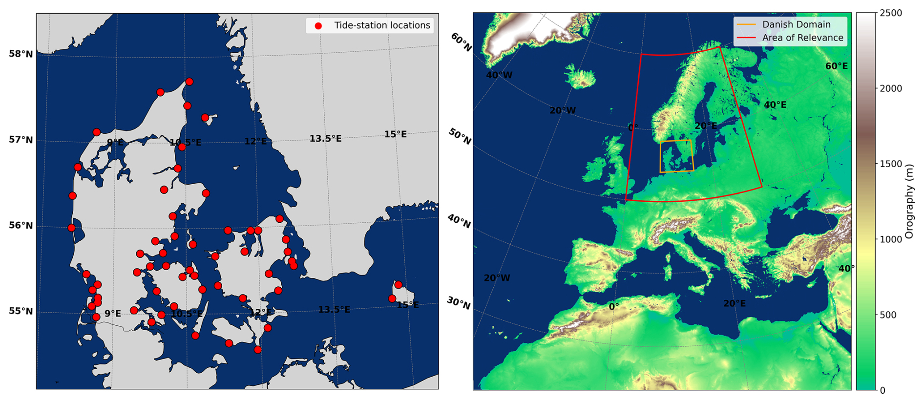
Figure 1 Map of Denmark with locations of tide gauge stations used to identify the high water level events (left) and full CERRA domain with surface topography (colour scale) and ocean mask (blue), as well as the “Area of Relevance” (AoR) and the Danish domain region in which water level impacts are sampled (right).

To identify and evaluate impact-relevant storm tracks, a set of significant storm surge events was compiled based on observed water level time series from Danish tide gauge stations (see locations in Fig. 1). We utilise detided water levels to ensure the algorithm focuses on significant surge events driven by severe storms rather than tidal influences, which vary considerably across the Danish coastline. Removing the tidal component enables a physically consistent and accurate identification of the surge peak timing, which is essential for initialising the storm-tracking window. While the relationship between tidal phases and wind-induced surges is critical for assessing total flooding severity, detiding isolates the meteorological driver for the purpose of algorithm development.

Storm surge events were selected using an empirical threshold corresponding to the 5-year return level at each station, ensuring that only significant extremes were included. To avoid double-counting of close extremes, a minimum time interval of 1.5 d between two events was imposed for both the same station and for events that occur across several stations. This selection process produced a set of dates in which coastal water levels exceeded thresholds indicative of high-impact events. We also performed a manual review of each case to exclude erroneous recordings and ensure that the elevated water levels were driven by extratropical cyclone activity rather than by other mechanisms, such as seiches or large anticyclones. As a result, six dates were excluded from the analysis due to the absence of an identifiable ETC driver. For all events, the time of impact was defined as the peak in the water-level time series, providing a physically consistent reference point for initialising the storm-tracking algorithm.

3 ETC tracking algorithm

The ETC detection and tracking algorithm of this paper begins with the user specifying a “time of impact”, e.g., the date and hour of a local storm surge event. The algorithm then searches for and tracks a potential ETC within a user-defined time window around the time of impact. Figure 2 presents a schematic overview of the core components within the ImpactETC1.0 tracking framework. The method is designed to systematically identify and isolate extratropical cyclones responsible for local surface impacts within a specified time window. Each stage in the workflow builds on the previous one, progressively refining the storm tracks from initial detection to final filtering. The figure outlines the logical flow between components, from storm centre identification to track linkage, spatial consolidation, and impact-based filtering. The sections are inherently independent in nature and thus can be seamlessly swapped for alternative approaches. The following Sect. 3.1–3.4 detail the implementation and rationale behind each step, while Sect. 3.5 provides an overview of the parameters involved.

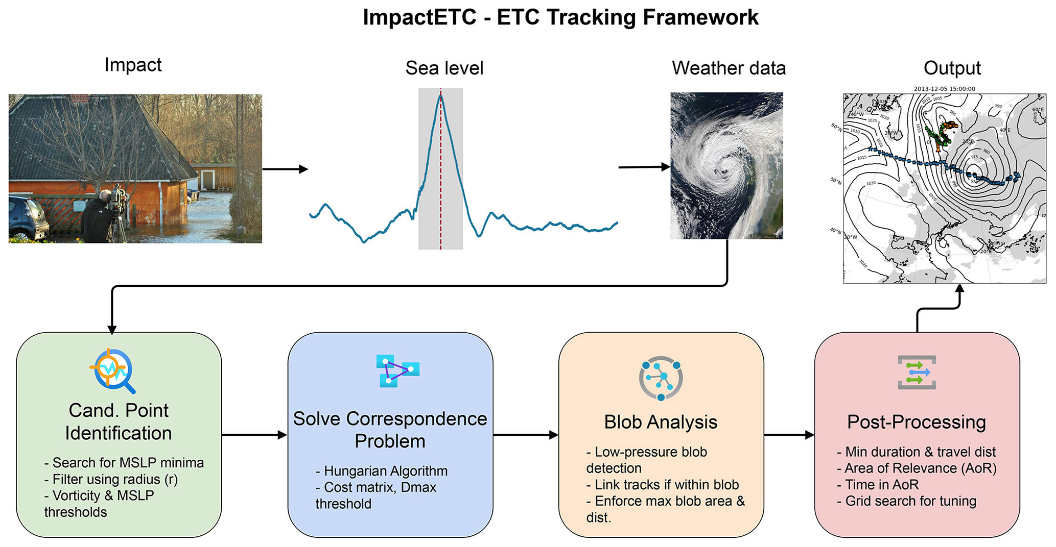
Figure 2 Overview of the ImpactETC1.0 framework for identifying ETCs linked to observed surface impacts (in order of arrows): Motivation of the study (impacts of Storm Bodil, December 2013, Photo: Martin Stendel), detided water level at a coastal station (±24 h impact window shaded), and associated ETC track. Bottom row (the four general stages of the storm tracking algorithm flow): (1) Candidate Point Identification (storm centres located by detecting MSLP minima and filtered using vorticity and spatial thresholds); (2) Solving the Correspondence Problem (storm centres linked across time using either a nearest-neighbour heuristic or the Hungarian Algorithm, with constraints on distance and cost); (3) BLOB Analysis – track discontinuities due to terrain or domain boundaries (resolved by reconnecting nearby low-pressure systems); (4) Post-Processing (tracks retained if they satisfy criteria for duration, travel distance, and overlap with a defined “area of relevance”, with parameters tuned through grid search), and (algorithm output, top right) impact-relevant ETC tracks capable of explaining localised storm surge or flooding events.

3.1 Identifying candidate points

Since the aim is to identify the relevant ETC that caused a local impact at a specific time, we first define a time window around the time of impact with start and end timestamps t_s and t_e, respectively. For the application of the algorithm to storm surge events in this paper, a time window of ±24 h was chosen around the beginning and end peaks of each storm surge event, yielding a minimum of 49 time steps per event. This search window is specifically balanced to ensure sufficient track continuity for the primary driver while minimising the inclusion of secondary, impact-irrelevant tracks that could introduce ambiguity during the automated calibration of post-processing parameters. This search window is highlighted in Fig. 3.

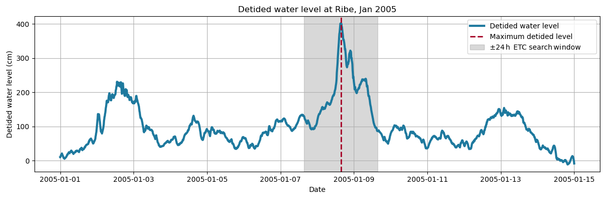
Figure 3 Time series of detided water level at Ribe, Denmark, during a storm surge event in January 2005. The dashed red line marks the time of maximum water level. The shaded region represents the ±24 h window around the peak used to identify and track the associated ETC.

Within this time window, the algorithm identifies candidate locations for the centre of an ETC by searching for local MSLP minima in the entire CERRA domain (Ridal et al., 2024). Across large spatial domains with high resolution grids, there are two issues: (1) the number of grid cells is large and simple local neighbourhood searches will generate multiple local minima, and (2) there may be multiple ETCs present within the domain at any given time. To handle the high resolution of the 5.5 km grid and avoid detecting excessive local noise, we employ a spatial partitioning approach rather than traditional grid coarsening or “upscaling”.

We first attempted using a kernel around each point to determine its status as a local minima, but this approach proved too computationally expensive. Instead, the goal is to upscale the original grid into coarser cells without missing any local minima due to overly large cells. The full domain is divided into non-overlapping square blocks where the diagonal length of each block is defined by the pruning radius, r. Using the Pythagorean theorem, we can derive the length of the squares from the diagonal, given by the pruning radius r as follows: $l=\sqrt{\frac{r^{\mathrm{2}}}{\mathrm{2}}}$. We proceed through the following steps (Fig. 4 shows the remaining potential candidate points after each step):

1. The algorithm determines the local MSLP minima within each spatial block, specifically identifying the individual 5.5 km grid cell with the lowest value. This ensures that the final coordinates remain faithful to the original data resolution without downsampling (Fig. 4a).

2. Remove local MSLP minima if any neighbouring upscaled cells within the pruning radius r contain a lower MSLP minimum (Fig. 4b).

3. Remove local MSLP minima with values above “MSLP_max” (Fig. 4c). While background MSLP fields can vary, a simple maximum cap is used to efficiently filter out high-pressure noise and weak systems unlikely to drive significant surface impacts. This computationally efficient approach is prioritised because candidate identification is already one of the algorithm's most demanding components. For the storm surge applications in this study, MSLP_max is set to a conservative value of 1010 hPa.

4. Remove local minima that do not have a ζ₅₀₀ intensity above ζ_500 min within a radius of 500 km, an approach consistent with established vorticity-based feature tracking methods (Gramcianinov et al., 2020, Fig. 4d). While this threshold may occasionally retain features from strong frontal structures that are not directly associated with an ETC core, its implementation is prioritised for computational speed at this high-demand stage of the processing. We opted against additional wind speed thresholds, as defining a single value applicable to both land and ocean surfaces risks unintentionally filtering out relevant candidate points in complex terrain.

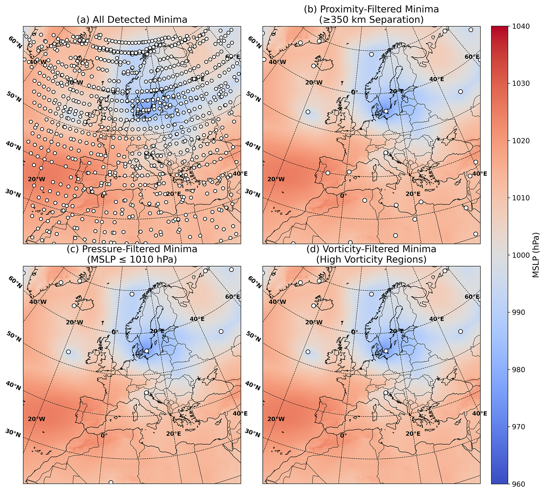
Figure 4 Visualisation of the progressive filtering of candidate cyclone centres using MSLP and 500 hPa vorticity criteria. From left to right, top to bottom: all local MSLP minima identified within upscaled grid cells. After applying radius-based culling, retaining only the lowest minimum within a defined neighbourhood. After removing candidates with MSLP values above the threshold MSLP_max. After further filtering out candidates lacking sufficient mid-tropospheric vorticity within a 500 km radius. The background shading depicts the MSLP field for context. The event is from 11 October 1997.

From these steps, we identify potential candidate points that represent the centre of an ETC. These will be used in the correspondence problem in the next step of the algorithm. The hyperparameters in these steps (r, maximum MSLP value at ETC centre, and minimum regional ζ₅₀₀ intensity) can all be fine-tuned for a given application of the algorithm. For the storm surge examples in this paper, we use the values r=350 km, ${\mathit{\zeta }}_{\mathrm{500}\min }=\mathrm{1.5}\times {\mathrm{10}}^{-\mathrm{4}}{\mathrm{s}}^{-\mathrm{1}}$, and MSLP_max=1010 hPa. The choice of r determines the size of the atmospheric structures that are preserved. It has to be large enough to filter away grid-scale noise and minor vortices if these are not of interest, but small enough to separate relevant features. If the user targets synoptic-scale systems, the pruning radius can reasonably be set to 500–1000 km, while smaller values are necessary to identify, e.g., secondary lows. The value of r can have a large impact on the computational efficiency of the algorithm, which will be investigated further in Sect. 5.2. In general, smaller pruning radii yield more candidate points, which in turn affects the algorithm's computational efficiency.

In a few rare instances, we have observed that two nearby candidate points have identical MSLP values in the CERRA data, which means that the aforementioned step 2 cannot select a unique point within the pruning radius. In this case, we have chosen to keep both points as possible candidates for the correspondence problem in the following section, rather than making an arbitrary selection between them. In Fig. 5, we show an example of MSLP minima points and 1 hPa isobar levels for the 11 October 1997 event, visualising the data in which the algorithm operates.

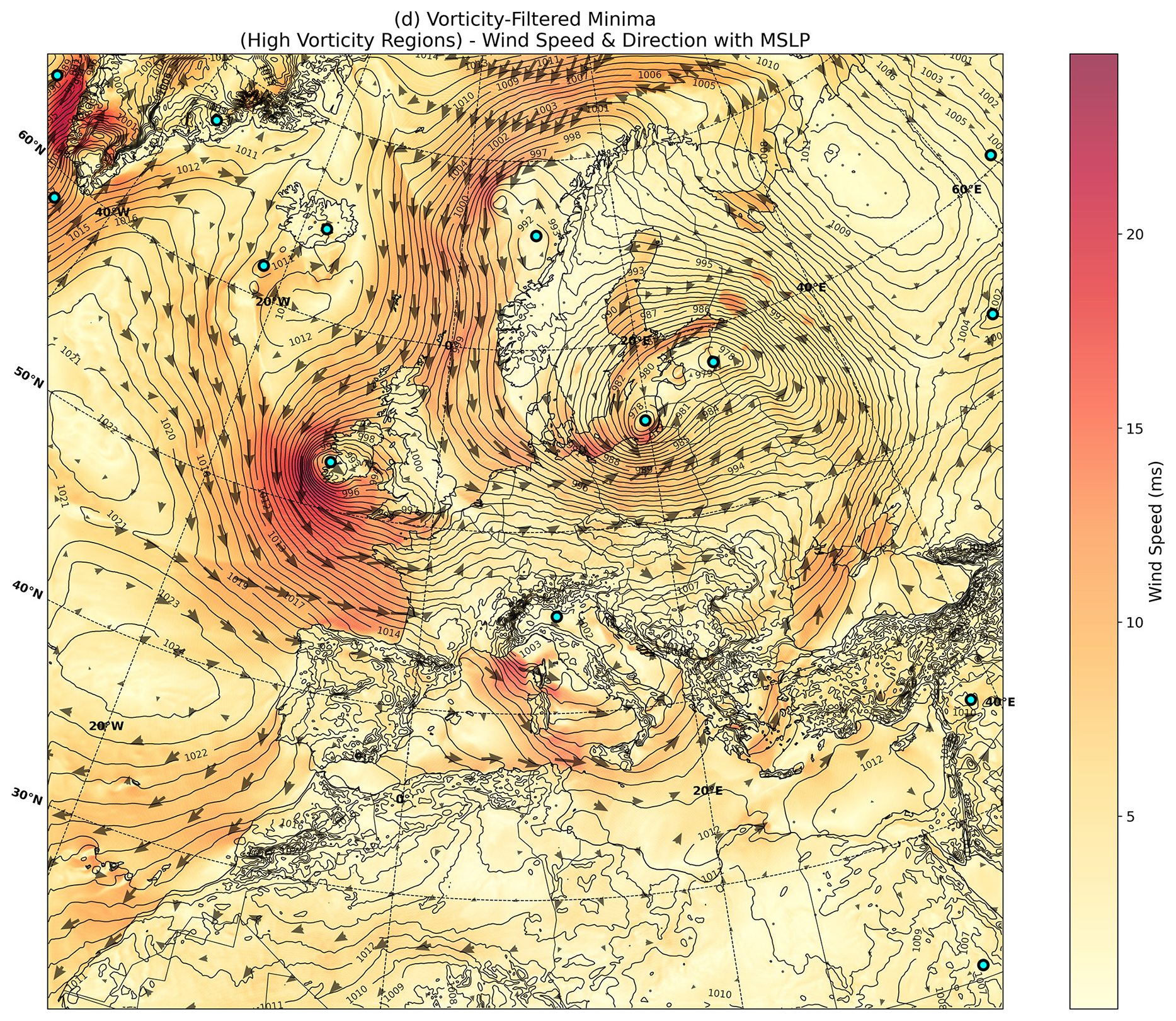
Figure 5 Joint plot of isobars (1 hPa scale), wind direction (arrows) and wind speed (color scale) for the 11 October 1997 event, to exemplify distinction of storm track centers.

3.2 Solving the correspondence problem

The candidate points found in Sect. 3.1 for each individual time step must now be connected through adjacent time steps to determine the storm tracks – a task known as the correspondence problem in the storm tracking literature (Walker et al., 2020). The general objective is to minimise the overall distance between the pairs of connected candidate points at time t_i and t_i+1. An added complication is that the number of candidate points in each time step is not guaranteed to be identical. If we define n and m as the number of candidate points at time t_i and t_i+1, respectively, then the problem can be either balanced if n=m or unbalanced if n≠m. A theoretical solution to this problem can be found through global optimisation. However, due to concerns about the computational requirements of global optimisation, it is common in current storm tracking algorithms to use a heuristic approach. This is often based on the nearest-neighbour approach, where one iterates through the candidate points at t_i and sequentially connects them to the candidate point closest in space at t_i+1. Usually, a threshold for the maximum possible travel distance of a storm centre between two time steps, D_max, is part of the heuristic algorithms. Heuristic-based approaches are not guaranteed to provide the correct solution, but they are computationally very fast.

In our tracking framework, we have implemented a global optimisation solution that avoids some of the pitfalls of nearest-neighbour heuristics. This type of correspondence problem is formally known as the “assignment problem” in optimisation theory, and it can be efficiently solved using the Hungarian Algorithm. The algorithm is well-studied in other fields, such as logistics (Seda, 2022) and scheduling (Zhang et al., 2024), and therefore we will only provide a general description here. The Hungarian algorithm begins with setting up a cost matrix, which here will be an n×m distance matrix, which represents the distance between all n candidate points at t_i and all m points at t_i+1. Equation (1) exemplifies how such a distance matrix is set up, with the leftmost matrix in Eq. (1) being n×m. The algorithm requires that the distance matrix be square, and since this is not guaranteed, the next step is to pad the matrix with phantom candidate points with a maximum cost (middle matrix in Eq. 1). We then apply a maximum allowable distance for a connection to be “realistic”, D_max. This parameter can be physically interpreted as a maximum allowable translation speed of the ETC centre, where reasonable estimates may be in the order of 100–150 km h⁻¹. However, the parameter can also be understood more conceptually as a “search radius” applied to the tracking variable (here MSLP). For the storm surge application presented in the Nordic region, we chose a value of 300 km, since complex terrain can cause the identified ETC centre to jump longer distances than what would be considered as physically reasonable. This maximum distance is implemented by censoring all matrix elements with values above D_max (see rightmost matrix in Eq. 1).

$$\begin{array}{}\text{(1)}& \begin{array}{rl}& \left[\begin{array}{ccc}\mathrm{2588}& \mathrm{105}& \mathrm{83}\\ \mathrm{6}& \mathrm{2640}& \mathrm{2510}\\ \mathrm{2395}& \mathrm{254}& \mathrm{112}\\ \mathrm{319}& \mathrm{2694}& \mathrm{2577}\end{array}\right]\to \\ & \left[\begin{array}{cccc}\mathrm{2588}& \mathrm{105}& \mathrm{83}& D_{\max }\\ \mathrm{6}& \mathrm{2640}& \mathrm{2510}& D_{\max }\\ \mathrm{2395}& \mathrm{254}& \mathrm{112}& D_{\max }\\ \mathrm{319}& \mathrm{2694}& \mathrm{2577}& D_{\max }\end{array}\right]\to \\ & \left[\begin{array}{cccc}{D}_{\max }& \mathrm{105}& \mathrm{83}& D_{\max }\\ \mathrm{6}& D_{\max }& D_{\max }& D_{\max }\\ D_{\max }& \mathrm{254}& \mathrm{112}& D_{\max }\\ D_{\max }& D_{\max }& D_{\max }& D_{\max }\end{array}\right]\end{array}\end{array}$$

Once the distance matrix is set up, made square, and censored, the algorithm finds the optimal solution by minimising the sum of distances across all connections. This is done through row/column reduction, covering zeros with lines, and matrix adjustments in the following steps:

1. Identify the smallest element in the matrix and subtract it from all elements, thus obtaining a matrix with at least one zero.

2. For horizontal and vertical lines through the rows and columns of the matrix, identify the minimum number of lines that would be required to cover all zeros.

3. If the number of lines is exactly the size of the matrix, then an optimal solution has been found. If it is smaller than the matrix size, an adjustment to the matrix is needed. The adjustment is to identify the smallest element h that is not covered by any line. Add h to all elements covered twice at the intersections of two lines and subtract h from all uncovered elements.

4. Repeat steps two and three until the number of lines required to cover the zeros is equal to the size of the matrix.

5. Select a set of connections that all have zeros. This is the optimal solution.

The connections found by the Hungarian Algorithm represent the solution that minimises the total sum of the connections between t_i and t_i+1. Computationally, in terms of big-O notation, it scales at O(n³). If multiple optimal solutions with the same objective value exist, the algorithm will return only one of them. In the case of storm tracking, with costs defined as the exact geographical distance between points, we deem it unlikely to occur.

The framework also contains a second option for solving the correspondence problem with a standard nearest-neighbour (NN) heuristic, which we will benchmark HA against. For the NN approach, we employ a greedy algorithm, which iteratively selects the valid minimum distance connection until all pairings are exhausted or exceed a predefined distance threshold D_max (see Algorithm 1):

Algorithm 1 Nearest neighbour heuristic for the correspondence problem.

Require:

Distance matrix $\mathbf{D}\in {\mathbb{R}}^{n\times m}$, maximum movement distance D_max

Ensure:

Assignment list 𝒜

1:

𝒜←∅

2:

while minimum value in D is less than D_max do

3:

Find $(i,j)=\arg min\mathbf{D}$

4:

Add (i,j) to 𝒜

5:

Remove row i and column j from D

6:

end while

7:

return  𝒜

The implemented HA and NN algorithms optimise connections with information from just two adjacent time steps, t_i and t_i+1. The limitation of such a one-step-at-a-time approach is that it can lead to a track breaking in two ways. First, if one of the timestamps along the ETC path is missing a candidate point, i.e., no local minima could be found. Second, even if a local minimum exists for all time steps, it can also have downstream implications for the connections that can be made later at t_i+2 onwards. Tracks can break if the “optimal” connection from t_i chooses a point at t_i+1 that is further away from the minimum in t_i+2 than one of its competing points, thus potentially not allowing for a connection to be made between t_i+1 and t_i+2. For such a scenario to occur, the user would have to specify a D_max value larger than the pruning radius, r, which would create the possibility of multiple candidate points within the D_max distance. To mitigate this second possibility, we introduce an additional algorithmic step to handle cases where tracks break because the required connection exceeds D_max.

3.3 BLOB analysis for resolving storm track fragmentation over complex terrain

In this study, MSLP is used to identify candidate points for the centres of ETCs. We chose MSLP over other possible tracking variables because of its close relationship to surface winds that drive storm surges. However, MSLP is a diagnostic variable, computed from the modelled surface pressure by estimating the sea level pressure under the assumption of hydrostatic balance (Pauley, 1998). Over complex terrain, this assumption often breaks down, e.g., over the Scandinavian mountains. As a result, artefacts and inaccuracies can arise in the MSLP field, potentially causing tracks to break into several fragments. A recurring example of this arises when an ETC crosses a mountain range: Candidate centres often appear to “stall” on the upstream side of the mountains, while a new candidate centre simultaneously appears downstream in the same time step. In this case, there are multiple alternative candidate points in the same time step for the same ETC system. This causes the track to break, resulting in a single ETC being misidentified as two separate systems. A tracking variable at higher atmospheric levels might be less prone to such issues, but it would also be less closely related to the surface impacts. We therefore introduce a novel track reconciliation step to allow for surface level tracking with MSLP while mitigating this type of track fragmentation. The reconciliation step is based on a BLOB analysis technique that performs synoptic-scale spatial continuity checks using the MSLP field.

We observed that when breaks occur, the upstream and downstream candidate points typically remain part of the same synoptic-scale low-pressure system, i.e. in close spatial proximity and with similar MSLP values. BLOB analysis leverages this by identifying contiguous low-pressure “regions” within a given MSLP range.

The method works as follows: for a given candidate point, we define a pressure range (e.g. ±5 hPa around its MSLP value). The entire MSLP field is then binarised, with grid points within the range set to 1 (inside a BLOB) and those outside set to 0. The result is a BLOB that represents spatially coherent low-pressure areas. For each time step, we check whether other candidate points fall within the same BLOB as the one containing the current candidate point. Figure 6a shows an example of a single ETC track that has broken into two fragments as it passed over the Scandinavian mountains. Figure 6b shows a snapshot at the time step where the track broke. Here, the yellow point is the candidate point under investigation, the red points are other ETC candidate points in the same time step, and the shaded areas are the computed BLOBs where MSLP values in the domain sit within a range of ±5 hPa of the MSLP value of the yellow point. In this case, there are three separate BLOBs in the domain but the algorithm only looks for red candidate points within the BLOB that contains the yellow point. The rest are disregarded.

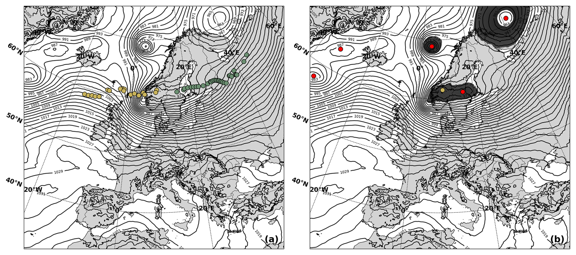
Figure 6 Illustration of the BLOB analysis step used for track reconciliation. Panel (a) shows an ETC crossing the Scandinavian mountains, where two valid MSLP minima appears in the same time step, which causes the track to break in two (yellow vs green). In (b), the BLOB analysis identifies spatially coherent low-pressure regions (BLOBs) and identifies candidate points within the same BLOB at the same time. Once identified, the method connects candidate centres upstream and downstream of the mountains to maintain a continuous storm track.

In certain edge cases, the BLOB's can become very large. To avoid false positives, we impose a maximum allowable BLOB bounding box of 3000 km and a threshold of 600 km for the maximum distance between two candidate points to be considered connected. When choosing the value of this second maximum BLOB candidate point distance parameter for a given use case, it is important to set it high enough to connect points within the same synoptic-scale system, e.g., in the range 500–1000 km. Its value should be larger than D_max to work as intended, but values much larger than 500–1000 km could risk merging distinct synoptic systems.

In simple cases, the discontinuity occurs at the end of one track fragment and the start of the next, which can then be merged. In more complex cases, two tracks may overlap temporally: the upstream track continues for a few time steps while the downstream track has already begun. The task then becomes choosing whether and when the jump from the first track to the start of the second track should occur. In these instances, we identify the first time step in which the two candidate points fall within the same BLOB. From that point onwards, we monitor both the continuations of the tracks and select the one that persists for the longest number of time steps as the final coherent track (see Fig. 7).

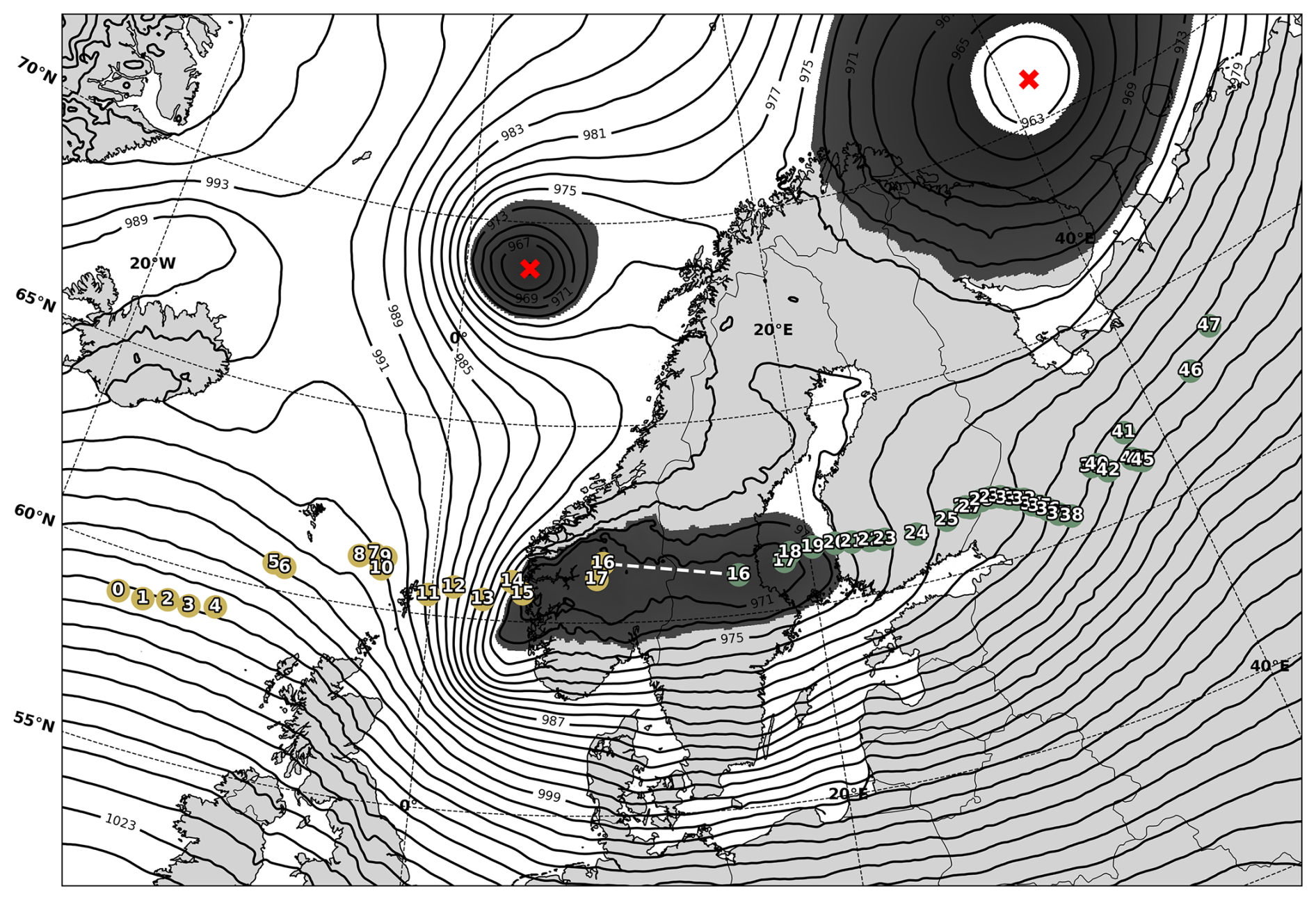
Figure 7 Example of track reconciliation between two fragmented tracks for the same case event as in Fig. 6. Points indicate MSLP minima and their assigned numbers show the time step during the event. The ETC moved from left to right in the image. At time step 16, the ETC reaches the Scandinavian mountains and the track breaks, leaving two tracks that both have valid ETC centre at time steps 16 and 17. The method creates a BLOB with a ±5 hPa range around the MSLP value at both points at step 16 (dark shaded area). Both points are within the threshold distance of the BLOB, and the algorithm jumps from the yellow to green track at point 16, because the white track continues on for a longer duration (green continues to time step 50, yellow only continues to time step 17). The red crosses denote other MSLP minima in the field, but since they are not within the same BLOB, they are ruled out as potential connections.

In the results section, we demonstrate the value of this track reconciliation step by showing how frequently it is used for the storm surge events in this study, how it affects the length of the final tracks, and how it prevents broken tracks from being filtered out in the post-processing steps described in the next section.

3.4 Post-processing of tracks

Within the impact time window, multiple ETC tracks are often present throughout the data domain. These tracks vary in length, duration, and spatial trajectory. Therefore, a crucial final step in any storm tracking algorithm is the filtering of tracks that are either insignificant or unrelated to the local impact.

In this study, we implement three options for post-processing tracks to identify the storm(s) that caused the local impact.

1. Impact-oriented calibration of standard post-processing parameters,

2. Nearest storm selection,

3. Gradient tracing.

3.4.1 Impact-oriented calibration of standard post-processing parameters

The first option allows the user to apply four criteria that an ETC track must satisfy to be considered relevant. These are standard post-processing criteria that are used in many different tracking algorithms in the literature:

• Minimum travel distance. The ETC must travel a minimum distance, measured as the total length of the track in kilometres.

• Minimum duration. The ETC must persist for a minimum duration, defined as the time between the first and last detected points along its track.

• Area of Relevance (AoR). The storm track must enter a predefined spatial area around the impact location.

• Minimum time in AoR. The ETC must spend a minimum amount of time within the AoR.

The first two criteria primarily eliminate short-lived or spatially limited tracks across the domain, while the latter two filter out tracks unlikely to have contributed to the local impact. While users can implement a circular AoR centred on a specific impact location, this framework utilises a rectangular AoR for programmatic efficiency when slicing 2D atmospheric fields. In cases like Danish storm surges, a non-symmetrical AoR is often physically preferable; for example, relevant ETCs may be located farther north or east in the Baltic Sea than to the west or south. Consequently, the AoR serves as a flexible, user-defined distance criterion, requiring the ETC to remain within a relevant proximity for a specified time window. Because the user provides the initial “time of impact” based on observed local water levels or winds, additional identification steps for the hazard itself are not required within the tracking loop.

In order to evaluate the sensitivity of the post-processing parameters and define a set of optimal parameters for our case study, a full grid search exploration of the parameter space is carried out, and the post-processing results are recorded. The parameter ranges applied for the grid search are as follows:

• Minimum travel distance. [0, 100, …, 1400, 1500 km].

• Minimum duration. [0, 1, …, 39, 40 h].

• Δ AoR. [−5, −4, …, 9, 10°].

• Minimum time in AoR. [0, 1, …, 29, 30 h].

We note that the AoR is centred on 60° N,15° E and initially spans from 50–70° N and 0–30° E. Here, the AoR change is in degrees with negative values decreasing the AoR and vice versa. The initial AoR encompasses the Baltic region and the North Sea (see the area highlighted in Fig. 1), since an ETC must enter this region to affect the water levels on the Danish coasts. In this study, we chose to define the AoR and the incremental changes in geographic degrees. Alternatively, this could have been defined in kilometres. This choice is possible for our AoR, as the effect from the varying length of a Δ1° is small (1–2 km in the zonal direction) due to the relatively small size and location of our AoR. Hence, we took a practical approach of using degrees, as this is how the CERRA data is given. However, for larger AoR and/or AoR located close to the poles, this is not a feasible solution and will be discussed further in Sect. 5.3.

To explore the parameter sensitivity, we use two metrics. The first metric assesses whether the post-processing filters yield the correct number of ETC tracks per impact event. To do this, we have undertaken the labour-intensive task of manually labelling the true count of ETC tracks within the AoR and the impact time window for all events in our case data. We then define a simple accuracy score for the evaluation, which we call the “Storm Count Accuracy” (SCA):

$$\begin{array}{}\text{(2)}& \mathrm{SCA}={\displaystyle \frac{\mathrm{1}}{n}}\sum _{i=\mathrm{1}}^n\mathrm{1}(y_i={\widehat{y}}_i)\end{array}$$

where y is the true number of ETCs, $\widehat{y}$ the predicted number given a set of post-processing parameter values, 1 $(y_i={\widehat{y}}_i)$ is an indicator function equal to 1 if correct and 0 if incorrect, and n is the total number of events. Please note that this metric only considers the accuracy of the counts of ETC tracks per impact event, and should not be confused with an accuracy assessment of the individual ETC track paths or a causal hazard attribution. Users of ImpactETC1.0 can do the same for their case implementations if the number of events to investigate is relatively small and manual labelling is deemed possible.

We recognise that developing a labelled dataset may not be desirable or possible for all applications of the algorithm, especially when evaluating many impact events. To still calibrate post-processing parameters rather than simply choosing values on an ad hoc basis, we tested a second metric that requires no manual work. If this second metric can calibrate parameter values to match those of the Storm Count Accuracy, it can be used for large-scale automated analyses. We define this second metric as the “Single Storm Score” (S):

$$\begin{array}{}\text{(3)}& S={\displaystyle \frac{N_{\mathrm{1}}-N_{\mathrm{0}}-N_{\mathrm{3}+}}{N_{\mathrm{0}}+N_{\mathrm{1}}+N_{\mathrm{2}}+N_{\mathrm{3}+}}}\end{array}$$

where N_i represents the number of events observed with i associated ETC tracks. This score rewards events with exactly one detected ETC (interpreted as a successful and unambiguous match), penalises missed detections (N₀) and excessive ambiguity (N₃₊). It treats cases with two ETCs as neutral, since we have observed this in our case example. The result is a simple, interpretable score ranging between −1 and 1, where higher values indicate better post-processing performance.

3.4.2 Nearest storm selection

The framework presents an alternative approach to calibrating filtering parameters using the Single Storm Score (S), which relies on the simple logic that the impact-relevant ETC was likely the one geographically closest to the impact location at the time of impact. This logic ensures that only a single ETC will be identified for each impact location. This simplifies post-processing by rendering the AoR redundant, thereby reducing the number of post-processing criteria from 4 to 2. The user is free to set the relevant parameters, and for this case study, we set “minimum duration” to 8 h and “minimum travel distance” to 300 km. If there are multiple eligible ETC tracks within the model domain, at the time of impact, the method calculates the distance from the impact location to each eligible track and selects the nearest.

3.4.3 Gradient tracing

A limitation of the “Nearest storm selection” approach is that it may not always be the track closest to the impact location that causes the event. Or it might be an interplay of multiple ETCs that cause it. As a third option, we therefore developed a “Gradient tracing” method based on the premise that the spatial pattern of the MSLP field contains important directional information about where the cause of the impact may originate. It applies the logic that the ETC that caused the impact probably holds the impact location within its “low-pressure basin”. Similar to the Nearest storm selection method, the “minimum duration” and “minimum travel distance” criteria are used to filter out micro-tracks, and in this case, are set to 8 h and 300 km, respectively. The gradient tracing method works by analysing the instantaneous MSLP field at the exact time of impact. It begins in the grid box where the impact location is and evaluates the 8 surrounding grid boxes. It then iteratively moves in the direction of steepest descent until it reaches a local minimum in the MSLP field. Once it has reached a local minimum, it evaluates whether this local minimum is a valid end point, defined as a point on one of the identified ETC tracks at the exact time of impact. If it is not a valid end point, it multiplies the MSLP value at the local minimum by a factor of 1.1, effectively raising the point above its neighbours, ensuring that a step into a neighbouring location is possible, and then moves in the direction of steepest descent again. It continues to iterate like this until it reaches a valid end point. The pseudo-code for the Gradient tracing method is defined in Algorithm 2. An example showcasing the method is highlighted in Fig. 8a, where the blue circle represents the starting location and the red squares represent a selection of the locations tracing has passed through towards termination at an ETC track, which are represented by the yellow stars.

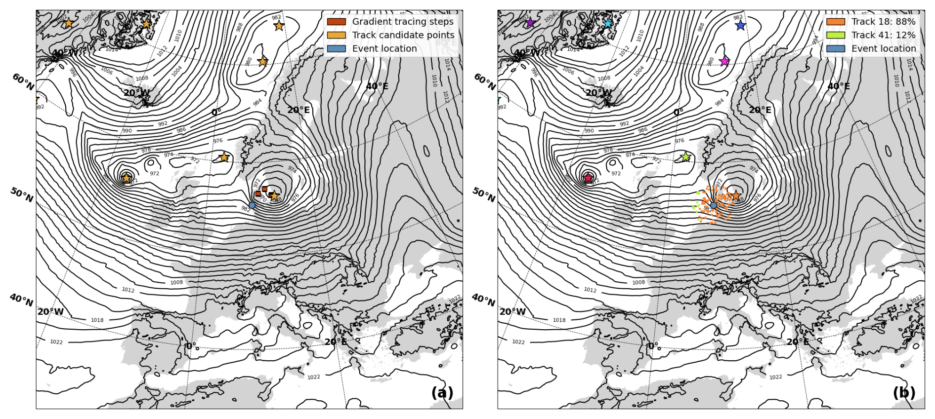
Figure 8 Visualisation of gradient tracing algorithm for the 26 February 2002 event where a storm surge happened at the city of Esbjerg. Contour lines show the MSLP field at the time of impact, and the star symbols represents identified ETC centres points. (a) The left panel shows the steps (red dots) that the gradient tracing method makes as it iteratively moves from the location of impact (blue dot) to one of the ETC centres. (b) The right panel shows how 100 starting points are sampled within a 250 km radius of the impact location. Each ETC centre (star) now has a distinct colour, and the colour of the starting points indicates which ETC centre, each starting point is assigned to with the gradient tracing method. The percentage numbers in the legend shows the proportion of starting points that end up at each ETC, here 88 % vs. 12 % for two nearby ETCs.

However, for some events, we observed that the initial impact location was located on a “ridge” in the MSLP field, where even small changes in the MSLP field determining which side of the ridge was stepped downward. We therefore introduced an additional option to include a measure of uncertainty to the identification of the impact-relevant storms. This is done by introducing spatial uncertainty in the impact location, from where the gradient tracing starts. Instead of only tracing from the exact impact location, we randomly sample 100 starting locations within a 250 km radius around the impact location, and perform gradient tracing for all of these. Doing so returns a percentage distribution of traces that terminate in each eligible ETC track, indicating how certain a specific ETC is to be the cause of the impact. A benefit of this is that this result can serve as an indicator of potential compound events when multiple ETCs interact to cause an event. Figure 8b shows an example where the exact impact location is represented by the blue circle, and the small squares surrounding the blue circle represent the randomly sampled starting points for the tracing exercise, with their colours representing the ETC track location where they terminated. As the legend shows, 88 % of traces end at one ETC, while 12 % end at another.

Algorithm 2 Gradient tracing for filtering of tracks

Require:

MSLP matrix $\mathbf{M}\in {\mathbb{R}}^{n\times m}$, maximum step iterations Iter_max, starting location radius S_radius, number of starting locations Z_max, storm center objects SC, each with attributes {loc,storm number}

Ensure:

Storm centers reached list 𝒜

1:

𝒜←∅

2:

Sample Z_max starting locations 𝒵 uniformly within radius S_radius

3:

for each Z_start∈𝒵 do

4:

Z_cur←Z_start,     step ←0

5:

while step ≤Iter_max do

6:

$N_{min}\leftarrow \arg {min}_{n\in \mathcal{N}\left(Z_{\text{cur}}\right)}\mathbf{M}\left[n\right]$

7:

if $\mathbf{M}\left[N_{min}\right]<\mathbf{M}\left[Z_{\text{cur}}\right]$ then

8:

$Z_{\text{cur}}\leftarrow N_{min}$

9:

else if Z_cur∈ SC then

10:

$\mathcal{A}\leftarrow \mathcal{A}\cup \mathit{\{}s.\text{storm number}\mathit{\}}$ {where s∈ SC s.t. $s.\text{loc}=Z_{\text{cur}}$}

11:

break

12:

else

13:

$\mathbf{M}\left[Z_{\text{cur}}\right]\leftarrow \mathrm{1.1}\cdot \mathbf{M}\left[Z_{\text{cur}}\right]$

14:

end if

15:

step ← step +1

16:

end while

17:

end for

18:

return  𝒜

3.5 Overview of parameters

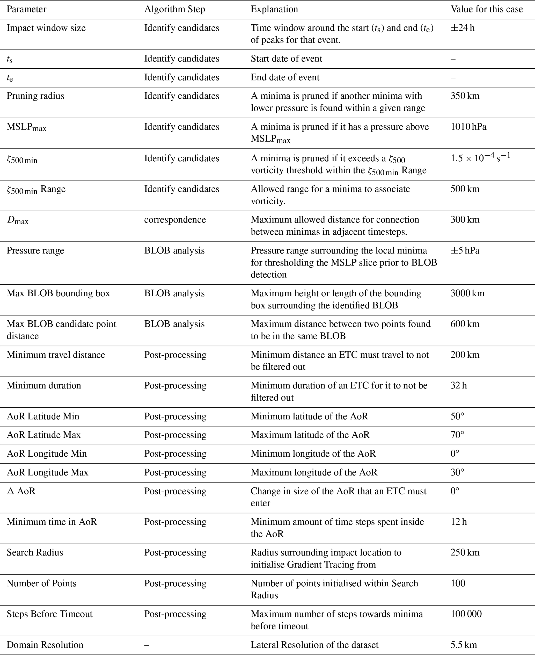
The full tracking algorithm contains many parameters and hyperparameters, some of which can be reasonably selected from knowledge of the physical system, while others need to be tuned for a given case area. In the literature on tracking algorithms, we often find a lack of (hyper-)parameter documentation, so here we present Table 1, which provides a full and transparent overview of the parameters in this algorithm.

Table 1 Overview of parameters in the full ETC tracking algorithm including explanation and the values used in the final setup for the case application.

4 Results

4.1 Correspondence problem: global optimisation vs. heuristics

Here we present results on the trade-off between solution quality and computational efficiency of the HA algorithm presented in Sect. 3.2 over a range of complexities of correspondence problems.

To explore the influence of problem complexity on NN and HA performance, we vary the pruning radius r used in the candidate point identification step. Smaller r-values yield denser point clouds and larger correspondence problems. We tested six radii: 100, 175, 250, 350, 500, and 700 km, evaluating the run time and three additional metrics that explore solution differences between HA and the greedy NN solution:

1. Number of correspondence problem solutions that yield different connections.

2. Number of additional connections in the global HA solution relative to the greedy NN solution.

3. Mean difference in the objective value of the correspondence problem, when the two solutions differ (in %).

During this analysis of the performance of HA and NN for the 37 impact events, a total of 1966 correspondence problems were solved, as summarised in (Table 2). Dates of the impact events are included in Table A1 in the Appendix.

Table 2 Comparison of Hungarian Algorithm (HA) and Nearest Neighbour (NN) for different pruning radii. The presented run times are to solve all 1966 correspondence problems across all 37 events.

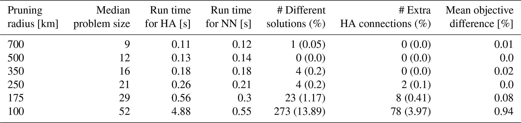
As the radius decreases, the number of candidate points and assignment options increases, which leads to greater problem complexity. Below a radius of 250 km, there is a sharp increase in different matches between HA and NN as well as extra HA connections. This happens because the pruning radius is significantly lower than the D_max value of 300 km, leading to multiple candidate points becoming eligible for connection. For larger radii and smaller problem sizes, the algorithms have very few legal moves, leading to similar solutions. At a 100 km radius, 13.9 % of correspondence problems yield different solutions using the NN method, and 3.97 % of the problems result in fewer valid storm track connections compared to HA.

Although the HA is significantly slower at small radii (e.g. 4.88 s at 100 km), it consistently achieves more connections between candidate points, which can be important for avoiding premature track termination. In applications where the domain is large and time steps are longer than the one-hour steps in CERRA (e.g. global reanalyses), similar complexity issues could potentially arise even with larger radii, making global optimisation even more relevant.

In our repository (Agertoft et al., 2026), we show an animation of the HA and NN algorithms connecting points through time for an illustrative event where the two solutions differ. In this specific example, the NN solution actually ends up with two tracks that cross each other in a single time step.

The D_max parameter is important for how the correspondence problem is solved with both HA and NN, as it controls the maximum connection distance between two candidate points in time. We have carried out a minor sensitivity analysis for D_max in order to assess its impact on the tracks that are formed. This can be found in the Appendix in Fig. A1. As expected, we observed that small D_max-values led to an increased number of tracks and generally shorter track durations, as fewer connections could be made across time steps. The sensitivity analysis showed that there was a smooth trend in the resulting number of tracks and length of individual tracks as D_max was varied. There was thus no obvious cut-off value to choose. We expect this to generally be the case for other areas and reanalysis time step lengths. However, to give some practical guidance for how to tune this parameter, we recommend that a good lower estimate for it would be a physically realistic value of how far the object being tracked can potentially travel in a single time step. The user can then increase the D_max value to pragmatically account for other effects, such as noise in the tracking field, terrain-driven discontinuities, etc. This is inherently a tuning problem that requires some trial and error testing.

4.2 Effect of track reconciliation

To evaluate the effect of the BLOB analysis technique for track reconciliation, we compare the full tracking system with and without the reconciliation step (see Table 3). This comparison does not assess the physical skill of reproducing the reconciled tracks as such. Instead, it quantifies how often reconciliation is applied and how it influences properties and survivability in the final track dataset after post-processing filters. The evaluation metrics are as follows:

1. The number of impact events in which at least one storm track survived post-processing out of the 37 total events.

2. The number of events with at least one surviving track that have used reconciliation out of the total number of events with at least one surviving track.

3. The number of tracks where reconciliation was used out of all surviving tracks in all events.

4. The number of reconciliations across all the surviving tracks versus the number of surviving tracks where reconciliation was used.

5. The average increase in track duration for tracks where reconciliation was used.

6. The average increase in track length for tracks where reconciliation was used.

Using the pruning radius of 350 km as an example, we notice that out of 37 total events, we have 37 events where at least one track survived the post-processing when utilising gradient tracing (see Table 3). The BLOB utilisation played a critical role in 19 events, affecting 19 surviving tracks. Across those 19 post-processed tracks, 28 reconciliations have occurred, meaning multiple surviving tracks have undergone more than one reconciliation. In summary, the use of BLOB analysis has ensured that a significantly higher number of tracks have survived post-processing. All 19 events in which BLOB analysis has been utilised have been manually investigated on an individual basis, and it has been found that the vast majority of the tracks in these events would otherwise not have represented reality satisfactorily.

Table 3 Summary of track reconciliation performance across different pruning radii, utilising gradient tracing post-processing. Metrics include the number of events with detected tracks, events and tracks where reconciliation is active, total number of reconciliations, and improvements in track duration and distance.

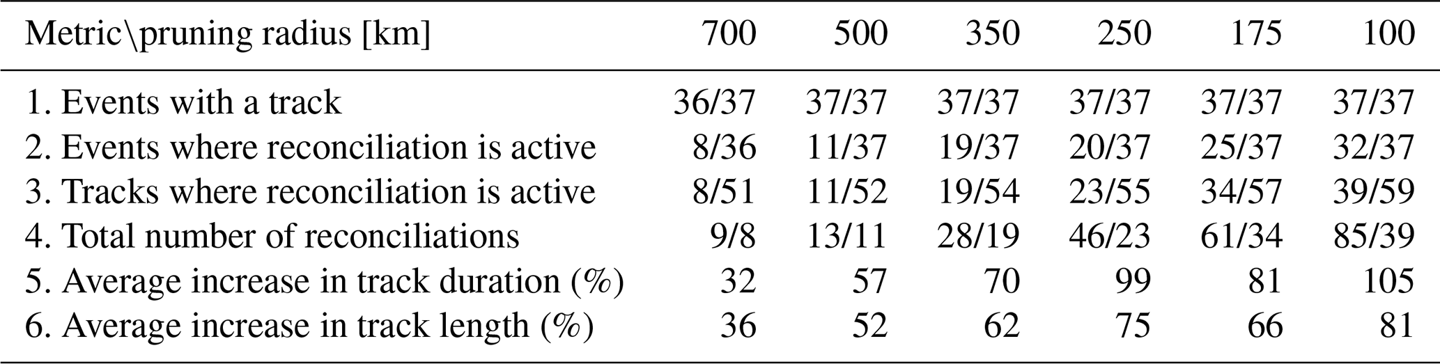
Figure 9 shows the geographical locations where BLOB reconstructions have occurred, as well as the distribution of the distances between candidate points connected by BLOB reconstructions. How active the BLOB step is depends heavily on the user-specified value of the pruning radius parameter. We therefore present BLOB reconstructions for the three different pruning radius values of 700 km (a, b), 350 km (c, d), and 100 km (e, f). In all cases, Max BLOB candidate point distance is set to a large value of 2500 km to analyse how connections are formed. The results generally show that smaller pruning radii lead to more blob connections because they leave many candidate points at each time step. The histograms of all three experiments show that there are a few reconstruction distances in the range of 1000–1600 km, which intuitively seems high. The vast majority of distances lie between the applied pruning radius (vertical, dashed line) and around 800 km, which is more reasonable given its intent to fix jumps across mountainous terrain. For the Nordic countries, we recommend using values of 600–800 km for this parameter, but users will need to re-evaluate this for other areas where these jumps may be smaller or larger.

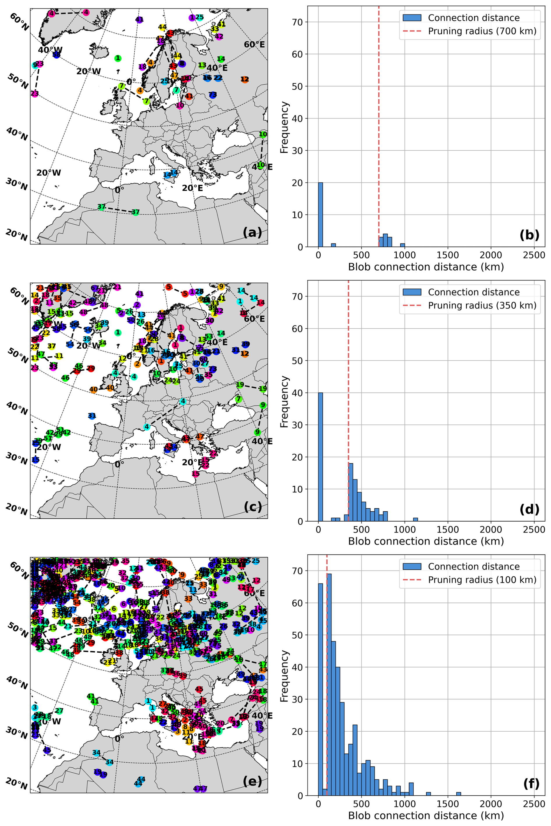
Figure 9 Overview of the BLOB track reconciliation connections for three pruning radius values of 700 km (a, b), 350 km (c, d), and 100 km (e, f). The left column of plots shows the geographic location of the reconstructed connections (a, c, e), where similar numbers at the point indicate the start and end of a connection. The right column shows a histogram of the distances of these connections (b, d, f) with a dashed vertical line that represents the pruning radius value.

Figure 9 also shows cases where reconstructed connections happen over very short distances. This shows up as reconstruction distances below the pruning radius value in the histograms (see Fig. 9b, d, f). These are formed during time steps t when multiple candidate points have the exact same MSLP value within each other's pruning radius. As explained earlier, we keep both points as candidates in such cases, but when the HA and NN algorithms then have to connect candidate points through time, there is a chance that the track ends prematurely, if the connection from t−1 to t is to one of the points but the continuation onwards from t to t+1 continues from the other point. The BLOB reconstruction handles this issue and connects the two broken track fragments.

4.3 Sensitivity and optimisation of post-processing parameters

Figure 10 shows the results of the parameter sensitivity analysis with both metrics. Each subplot in the figure shows the sensitivity of ETC detection to one of the four post-processing parameters. Given the discretisation of the chosen grid search for each parameter, there are a total of 325 376 possible combinations of the four parameters. The plots show the median, the 5th and 95th percentiles of the score values across all combinations. The results show that ETC detection is most sensitive to the size of the AoR (Fig. 10a), time in AoR (Fig. 10b), and the minimum travel distance (Fig. 10c). Notably, there is the special case where minimum time in AoR equals 0, meaning that an ETC does not need to enter the AoR for detection, which leads to a large drop in performance (Fig. 10b). The large distance between the 5th and 95th percentiles, as indicated by the shaded areas, shows that the same parameter value can lead to very different post-processing performance depending on the values of the other post-processing parameters. Thus, there is a strong dependence between parameters; e.g., the size of the AoR and the minimum time in the AoR are closely related.

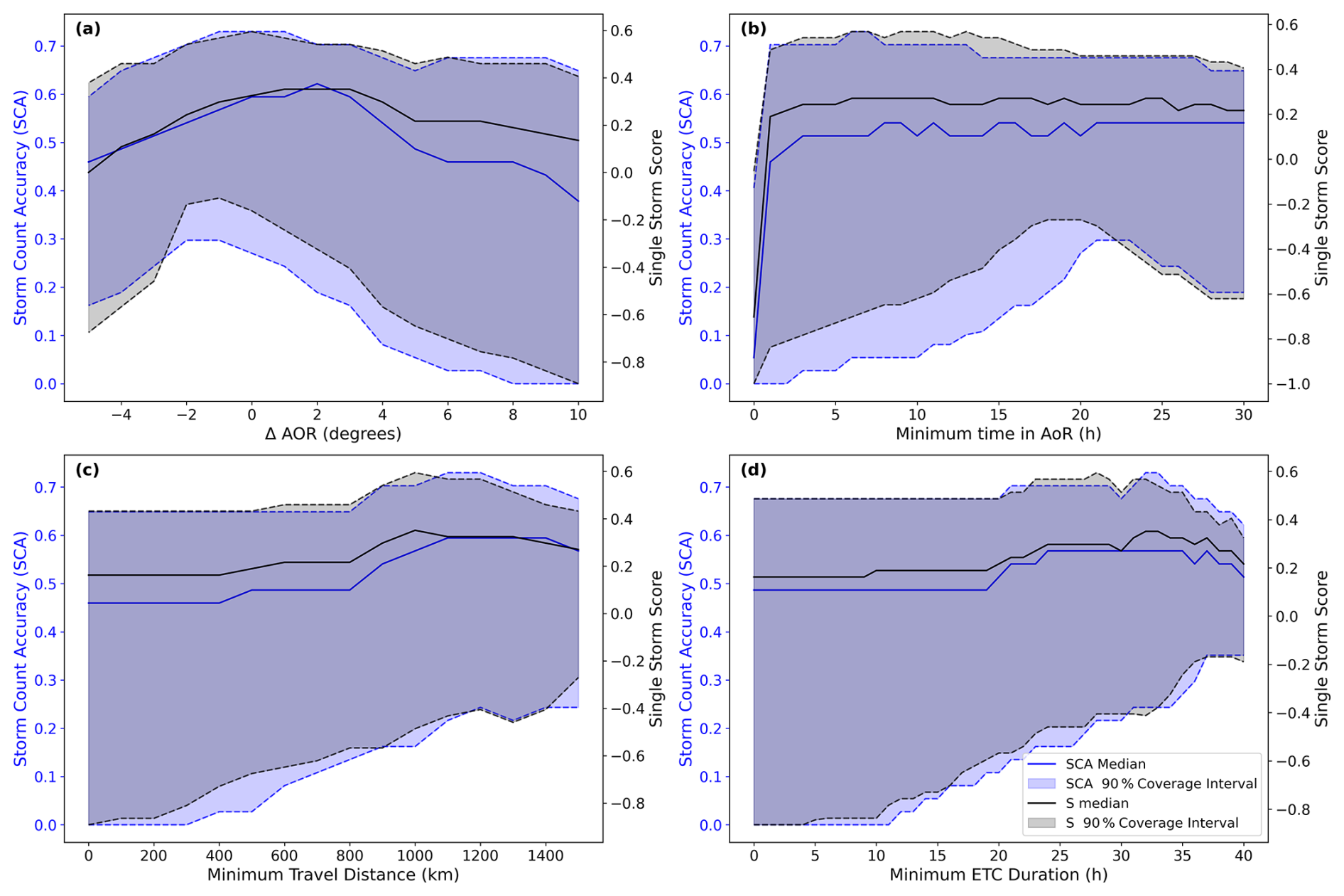
Figure 10 Sensitivity of the ImpactETC1.0 algorithm's performance to key post-processing parameters. Each panel shows the impact of varying a specific parameter on two metrics: the S score (black) and SCA relative to historical impact records (blue). (a) Sensitivity to Δ AoR in degrees, (b) number of time steps required within the AoR, (c) minimum travel distance of detected ETC tracks in km, and (d) minimum ETC duration in hours. These experiments highlight trade-offs in tuning filtering parameters.

Figure 11 shows the marginal and joint distributions of the Storm Count Accuracy and Single Storm Score after the values of both scores have been min-max normalised to fit the same 0–1 range. The marginal distributions follow each other closely with small deviations in some ranges. The joint distribution confirms that the Single Storm Score yields normalised values similar to the Storm Count Accuracy. This, combined with the general agreement of the scores in Fig. 10, shows that the Single Storm Score is good at approximating the Storm Count Accuracy and thus suitable for impact-focused calibration when manual labelling is not possible.

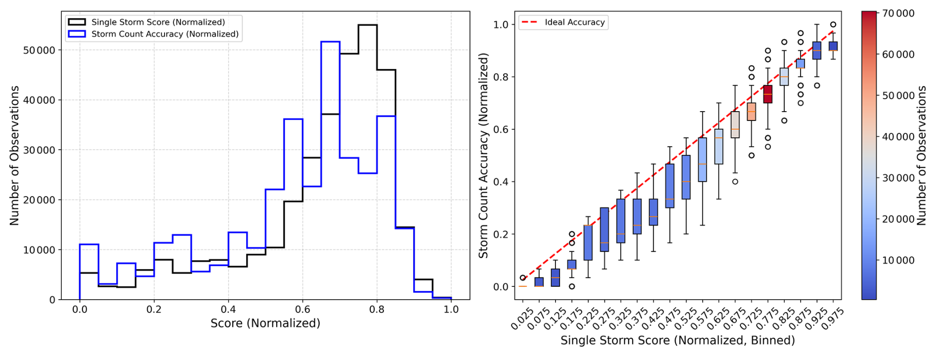
Figure 11 Comparison of marginal (left) and joint (right) distributions of the Storm Count Accuracy and the Single Storm Score after both scores have been min-max normalised to fit 0–1 ranges. The joint distribution is shown as corresponding Storm Count Accuracy values for discretised bins of Single Storm Score values. The red dashed line indicates the ideal 1:1 relationship. Colour shading in box plots indicates the number of observations per bin.

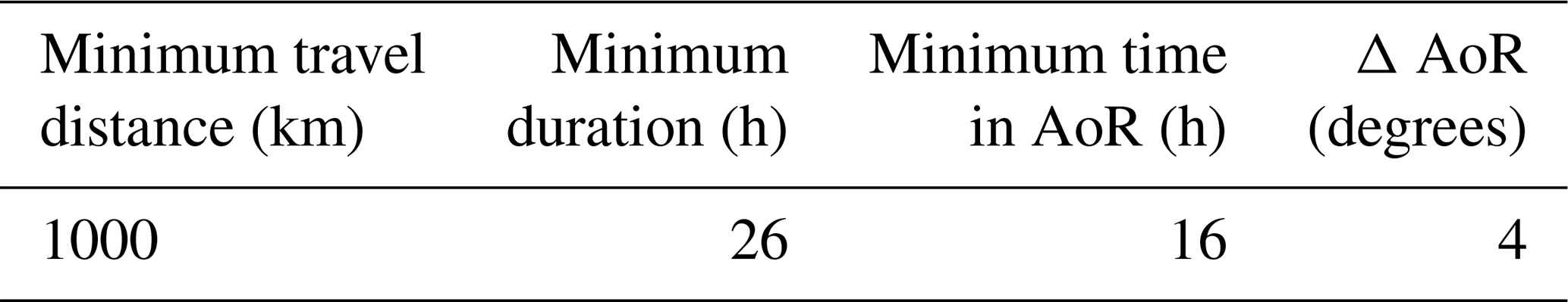
For the presented case of ETCs that produce storm-surge events, we select the parameter set that yields the best Single Storm Score. Given the grid search discretisation, there are 325 376 possible combinations of the four post-processing parameters. In the case presented, 20 unique parameter sets yielded the same score. We selected the parameter set that was closest to the median of each parameter (see values in Table 4), thus avoiding extremes or accidentally fortunate local minima. We note that this method for selecting parameter combinations is only suitable if the possible combinations are centred in nature. If they had, e.g. been clustered in two different areas of the parameter space, the user would have to devise another way to select the final set. It is worth noting that even though all 325 376 parameter combinations were simulated in a brute-force manner, this still only took ∼ 3 min to complete on a standard laptop. This highlights that calibrating post-processing parameters is a simple, fast step that should be performed.

Table 4 Optimal post-processing parameter values identified for the storm surge case in this study.

5 Discussion

5.1 Strengths and limitations of the tracking algorithm

To assess the quality of the identified ETC tracks, we present a set of representative storm surge cases here. Figure 12 shows six examples of well-defined ETC tracks that exhibit consistent spatial progression, relatively smooth trajectories, and alignment with the underlying MSLP field. These cases demonstrate the algorithm's ability to capture the temporal and spatial evolution of ETCs, even as they traverse complex regions with steep topography and land-ocean boundaries.

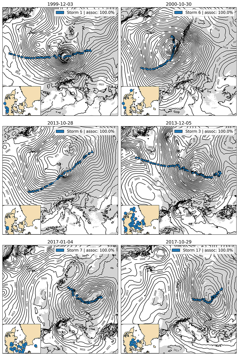
Figure 12 Six examples of well-defined, successfully identified ETC tracks by gradient tracing post-processing. Blue dots mark the time evolution along each track, and stars indicate the initial position of each track. The background shows the MSLP field at the median time step of each track, providing synoptic context for storm positioning and structure. For each example, the insert maps show locations of the water-level gauges where storm surges were found.

In contrast, Fig. 13 highlights six events that illustrate the challenges of the algorithm. In these subplots, tracks that are coloured red were deemed impact-irrelevant despite manual inspection of the events suggesting that this was the wrong decision. Other colours than red show tracks that were deemed impact-relevant and has an uncertainty estimate associated with it in the legend of each subplot. For the storm surge case of this paper, we chose 300 km as the value of D_max but several of the events in Fig. 13 ends up with fragmented tracks because this value is too low. This is true for the two red track fragments in the 29 January 2001 event and the two red fragments in the 18 November 2004 event. The 8 January 2005 consists of two small red track fragments and two larger ones coloured in blue and orange, however, manual inspection revealed that these all belong the same ETC. It was again a too small D_max value that caused the break between the second red fragment and the blue fragment, and again between the blue and orange fragments. If a user of the framework is particularly interested in a single-event analyses of these events, it would be straightforward to experiment with new D_max values until the desired track is obtained. However, for batch processing of many events at once where manual single-event inspection is deemed unfeasible, it is a limitation of the framework that the user has to specify a single D_max value for all cases. Based on performing many experiments with the algorithm ourselves, we find that no single parameter set performs perfectly at all events.

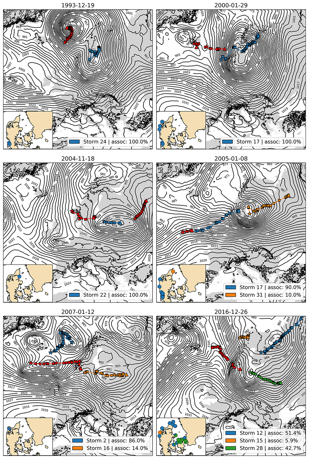
Figure 13 Six examples of ETC tracks that show the limitations of the algorithm, e.g. track splitting, short-lived centres, non-smooth movements, or secondary impact-irrelevant tracks that survive post-processing. Blue tracks are successfully identified ETCs, orange and green denote secondary impact-irrelevant tracks that survive post-processing, while red shows tracks that are impact-relevant but were filtered out. The gradient tracing approach has been used to quantify, in percentages, the storm tracks relation to impact locations for each ETC event (lower-left insert maps, coloured by storm). In our repository (Agertoft et al., 2026), we provided the animations of these six events.

During the 12 January 2007 event, three separate ETC were present at the time of impact (coloured red, orange, and blue). While the red and orange tracks may look two fragments of a single track because the red ends close to where the orange starts, they were in fact two separate systems. At the time of impact, the red track was located west of the impact location, the orange track to the east, and the blue track far north between Iceland and Norway. Manual evaluation of the event suggests that the impact is caused by the combined effect of the red and orange tracks that together produce strong MSLP gradients (and related westerly winds) in the North Sea. The MSLP field in the still image of the figure shows that the impact location sits on a ridge in the field. 86 % of the initialised gradient tracing attempts traces the impact northwards on the eastern side of the Scandinavian mountains all the up to the blue ETC track, and not westwards towards the red track, which there is left undiscovered as an impact-relevant ETC. This example shows that the gradient tracing method in some special cases can be vulnerable to small-scale variations in the MSLP field, even when it initialises many tries in a 250 km radius around the impact location.

In the 26 December 2016 event shows a unique failure of the framework. Here, manual inspection of the event revealed that the two red fragments and the green fragment belonged to the same ETC, which originated in the North Atlantic and crossed the Scandinavian mountains in a northwest-southeast movement, terminating in Eastern Europe. However, the framework was not able to connect these fragments because there are several time steps where no ETC centre candidate points could be found as the ETC crossed the Scandinavian mountains. This happened because the MSLP field became very vauge without a well-defined minima. Between the second red and the green fragments there was a gap of four time steps without a minima, which incidentally was right at the time of impact of several of the impacted locations shown in the inset at the lower left corner of the 26 December 2016 event. Because the combined red-green fragmented track did not exist in the four time step gap, the gradient tracing algorithm traced the impacts to the orange and blue ETCs that were located further away.

5.2 The value of global optimisation to solve the correspondence problem

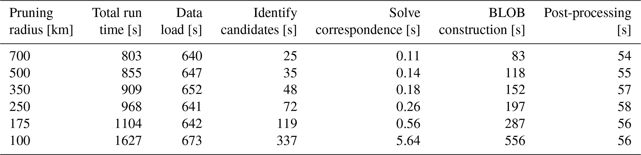
A central question when choosing between a heuristic and a mathematically exact solution to the correspondence problem is whether the additional computational cost of global optimisation meaningfully affects overall algorithm performance. Table 5 shows the total computational run times for serial execution of ImpactETC1.0 on all 37 events. The runtime is divided into the main steps of the framework and tested across several pruning radii (i.e., r-values), which lead to different problem complexities to solve. This analysis shows that solving the correspondence problem with the HA accounts for only a small fraction of the total computational time, especially compared to more time-consuming components such as data loading and candidate point identification. Even at the highest level of correspondence complexity (100 km pruning radius), solving the correspondence problem remains a minor contributor to total run time compared to candidate point processing and BLOB analysis. The analysis in Table 2 shows that the differences between HA and NN drastically increase with the complexity of the problem (small pruning radii), and that HA enables additional connections. While we here investigate tracking of ETCs, which exist at large spatial scales, it is likely that HA would be even more suitable for tracking smaller atmospheric objectives and for tracking in noisier fields. This is something future research could target.

Table 5 Breakdown of algorithm run time (s) across individual framework components for different candidate point pruning radii, r. Columns show total run time vs times spent on data loading, candidate identification, solving the correspondence problem, BLOB construction, and post-processing utilising gradient tracing. Values are averages over all events, highlighting how pruning radius affects computational demands and the relative contributions of each algorithm component.

5.3 Future improvements and considerations for broader application

While the ImpactETC1.0 framework demonstrates robust performance in identifying impact-relevant ETC tracks, there are several avenues to further improve its performance and computational efficiency.

• Computational efficiency. Data loading consistently dominates runtime across all pruning radii, and while optimised data handling could reduce this component, it will likely remain a significant fraction of total runtime. The candidate identification step is already quite scalable, but it might be possible to avoid excessive block comparisons with further developments. For track reconciliation, there are likely gains to be made, e.g. by adding a distance-based pre-check before BLOB initialisation, which would reduce unnecessary BLOB constructions. The current implementation of the framework is serial but future developments could exploit parallelisation on modern computing infrastructure. Since the framework is event-focused by design, it would be straightforward and efficient to analyse independent impact events in parallel. Specific algorithmic steps could further benefit from parallelisation, especially the candidate point identification and the BLOB construction, since they treat individual time steps independently. The track reconciliation based on the constructed BLOBs would still have to remain serial to avoid conflicts during merging of track fragments. The grid search employed for the impact-oriented calibration of post-processing parameters is embarrassingly parallel. The “nearest storm selection” and “gradient tracing” post-processing options treat each impact location independently and could similarly be parallelised.

• Improved tracking. In terms of the quality of the final tracks, more research could be done on how to refine the track reconciliation step, for example, as seen in Fig. 13 for the 6 December 2016 event, where the BLOB analysis makes the wrong connection because there is a single time step where no candidate point is found on the correct track. It might be worth exploring how to incorporate multiple adjacent time steps into the BLOB analysis, rather than limiting reconciliation checks to simultaneous candidate points. Or alternatively to allow for temporal gaps during the HA/NN solutions to the correspondence problem (Ullrich et al., 2021; Peréz-Alarcón et al., 2024). It could also be worth testing the implementation of user-defined masks of high-uncertainty areas, such as mountain ranges, where the BLOB analysis is given more freedom in space and time to make the right connections. This extension would enable a more realistic identification of track jumps across complex terrains or during rapid ETC evolution. There may also be improvements by using ETC tracking information at higher pressure levels, such as 700 hPa, to improve the continuity of surface-level tracks during reconciliation. While the BLOB-based reconciliation step is crucial for avoiding premature track termination, it sometimes causes irregular jumps between points on the track. It would be interesting to explore ways to smooth tracks around reconciliation jumps. This could potentially also be guided by information at higher pressure levels.

• Post-processing. The presented framework introduced three post-processing methods intended to filter out impact-irrelevant ETC tracks. Future research could further investigate the differences between these methods, e.g., comparing under which conditions the gradient tracing and nearest storm selection fail. There is also scope for more research on improving the robustness of the gradient tracing method against small-scale effects in the MSLP field. Future research could further investigate the version of the gradient tracing method with many initialisations to identify compound events where multiple ETCs interact to produce the impact. In this study, we investigate storm surge impacts driven by surface winds, which is a phenomena that is closely related to the local MSLP gradients. Other types of impacts, such as extreme precipitation events where, e.g., atmospheric rivers can cause impacts to extend far away from the ETC centre, further research will have to develop additional methods to attribute an impact to a specific nearby ETC.

• Additional features. To deepen the physical interpretation of ETC evolution, associating additional properties – such as MSLP at ETC centre, vorticity, wind speed, or gusts – along identified tracks would allow classification of different stages of the storm life cycle, including genesis, intensification, mature phase, and occlusion. Even though these additional features could help limit the unintended removal of short-lived yet impactful systems that drive significant extremes, investigating such variables would likely increase the algorithm's computational demand. Future iterations could also incorporate local wind direction criteria. In complex coastal regions like the Danish straits, specific wind directions are primary drivers of surges; however, defining these thresholds requires significant a priori local oceanographic knowledge.

• Limitations of 1-D tracking and Lagrangian analysis. The main feature of the framework presented here is that it is impact-oriented, thus distinguishing between impact-relevant and irrelevant ETCs. This distinction depends on the type of impact studied, defined by the timing and location of the maximum impact, and it is the main purpose of the post-processing steps. We present three post-processing methods, all based on the assumption that the ETC responsible for the impact is close to the impact location and at the time of maximum impact. This assumption is softened in the Gradient Tracing method, as a stronger ETC farther away may be chosen instead. However, this still implicitly assumes that the impact is caused by phenomena close to the core of the ETC. Certain types of impacts, such as pluvial flooding from precipitation, may occur far from the core. For those types of impacts, the ETCs identified with our framework will most likely be the impact-relevant ETC, but without explicitly associating the tracks with the atmospheric phenomenon (i.e., precipitation) causing the impact type (i.e., pluvial flooding), it cannot be determined for certain. This requires a deeper analysis of drivers of the hazards for each individual event and is beyond the scope of the present study. This lack of information about the spatio-temporal evolution of the atmosphere is a limitation not only for the framework presented here but also, in general, for point-wise Lagrangian analysis and 1-D tracks. This could be incorporated in a future version of the algorithm.

• Broader applications. We believe that ImpactETC1.0 is broadly applicable to other case areas. Users applying the framework to other reanalysis datasets or to different geographic regions should consider recalibrating key parameters, especially candidate detection thresholds, correspondence distance limits, and AoR size, to account for differences in data resolution, domain size, and regional storm climatology. The framework currently only works for data on structured grids but future work could explore how to adapt it to data on unstructured meshes, where especially the candidate identification and BLOB reconciliation steps would need improvements.

6 Conclusion

In this study, the ImpactETC1.0 storm tracking framework is introduced, bridging the gap between large-scale dynamics and localised hazards by linking extratropical cyclone (ETC) tracks directly to surface impacts. Novelties of the paper include the use of global optimisation via the Hungarian Algorithm, BLOB-based track reconciliation (efficient, e.g., over complex terrain), several post-processing methods, and an automated validation metric that helps the user identify the storm(s) that caused the impact.

The framework is exemplified using the 5.5 km hourly CERRA reanalysis data for the 1991–2020 period, and the impact-based selection was validated against historical storm surges that exceeded 5-year return levels (here, 37 events), using a ±24 h search window around peak sea levels. On this basis, the algorithm isolates the primary storm track(s) relevant to the storm surge while effectively filtering out irrelevant ones.

To solve the correspondence problem, the framework uses the Hungarian Algorithm (HA) for global optimisation, and validated this approach against the commonly used nearest-neighbour approach. The HA approach provided more connections, especially under conditions with many candidate points, and, despite its increased computational complexity, remains highly efficient, accounting for less than 1 % of the total system runtime.

To address storm-track fragmentation over complex terrain, a BLOB-based reconciliation identifies contiguous low-pressure regions to reconnect broken tracks. At the chosen pruning radius of 350 km, the BLOB reconciliation increased the average track duration by 70 % and the total length by 62 %, preventing, e.g., premature termination over the Scandinavian mountains.

Two post-processing options – nearest storm selection, and gradient-tracing – were introduced and evaluated alongside automatic calibration with the “Single Storm Score,” which can be used to avoid manual tuning or ad-hoc parameter selection. While data loading currently accounts for a substantial share of processing time, the framework’s modular design enables future parallelisation and operational scaling.

For future application, ImpactETC1.0 offers a scalable tool beyond storm surges alone for assessing additional applications such as wind damages, providing a robust, automated methodology for historical hazard analysis and future climate adaptation planning. All together, these methodological advances enable skilful reconstruction of the ETC tracks, even in regions with complex topography and during rapid storm development, while maintaining relatively low computational demands.

Appendix A

Table A1 Start and end dates of events, if only one station was hit then start date equals end date, if not then multiple stations were hit sequentially and start date represents the peak of the earliest station hit, and end date represents the peak of the last station hit in that event. Timestamp highlights peaks of event.

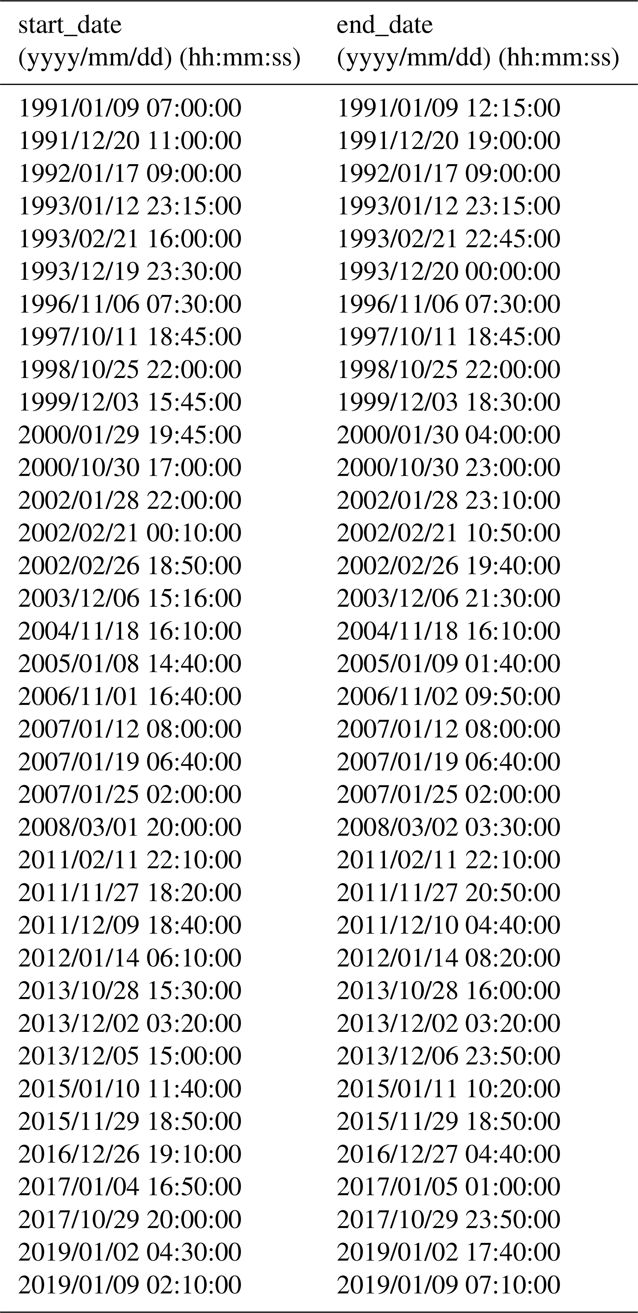
Table A2 Summary of track reconciliation performance across different pruning radii, utilizing Single Storm Score post processing. Metrics include the number of events with detected tracks, events and tracks where reconciliation is active, total number of reconciliations, and improvements in track duration and distance.

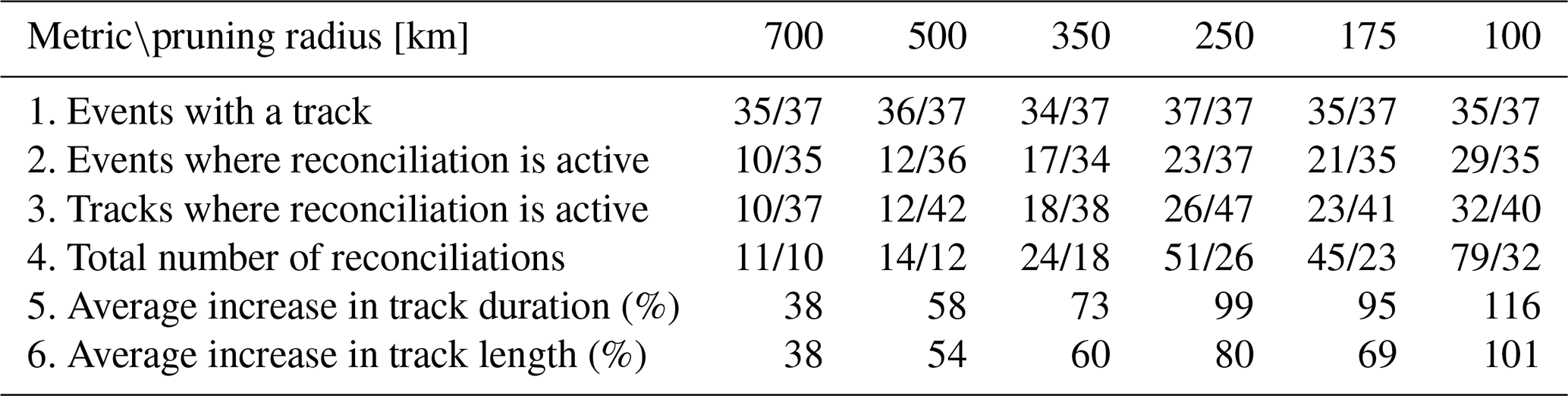
Table A3 Summary of track reconciliation performance across different pruning radii, utilizing Closest Track post processing. Metrics include the number of events with detected tracks, events and tracks where reconciliation is active, total number of reconciliations, and improvements in track duration and distance.

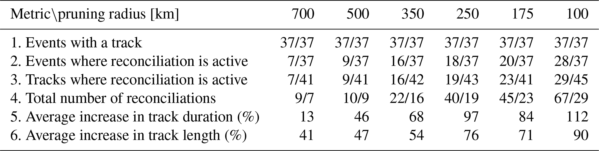
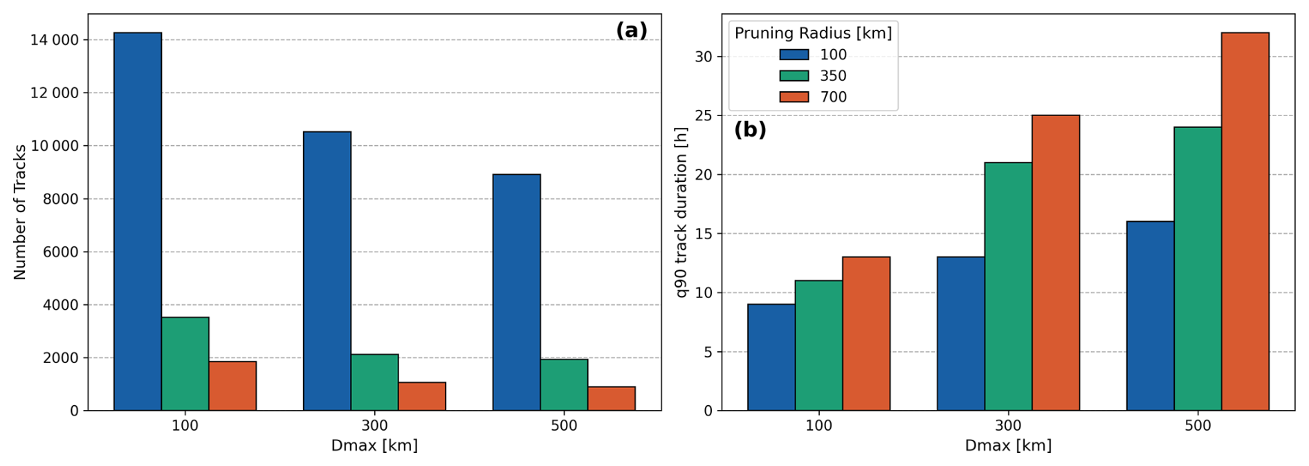
Figure A1 Sensitivity of D_max and Pruning radius represented through two track metrics. (a) shows the number of tracks under different D_max and Pruning radii combinations, (b) shows the q90 track duration in hours under different D_max and Pruning radii combinations. These experiments highlight trade-offs in tuning filtering parameters.

Figure A1 shows the D_max sensitivity analysis, where D_max was varied for two different pruning radius scenarios. The metrics selected for studying the effect on the formed tracks were (a) the number of tracks, and (b) the track duration. The sensitivity analysis was conducted on the correspondence problem-step of the algorithm, which is executed before the BLOB-based track reconciliation and the post-processing steps, which also have significant influence on the final track properties. These two steps connects small track fragments and filters minor, impact-irrelevant tracks away, respectively. These steps were not executed for this minor sensitivity analysis to isolate the influence of D_max, and this resulted in many small tracks. Most of which would be filtered out later. We therefore chose to plot the 90th quantile of the track duration rather than the mean or median track length to better see the D_max influence.

For good measure, we note that neither an increased number of tracks nor an increased q90 track duration is inherently desirable by themselves, as a high number of tracks implies many smaller tracks with severed connections and an abnormally high q90 track duration would imply tracks with connections that are not representative of the underlying system.