Global climate modeling with improved precipitation characteristics by learning physics (GRIST-MPS v1.0) from global storm-resolving modeling

This study develops a machine learning (ML)-based physics parameterization suite trained on 80 d global storm-resolving model (GSRM) simulation data (5 km), with the aim of replacing all conventional physics tendencies in a general circulation model (GCM, 120 km) for real-world simulations with realistic surface topography. The GSRM data are generated using the Global–Regional Integrated Forecast System (GRIST) and subsequently coarse-grained, after which the residual method is applied to derive the corresponding GCM physics tendencies. The resulting workflow relies on standardized pressure-level variables as input features, enabling the GCM – through physics–dynamics coupling – to effectively emulate the multiscale flow interactions captured by the GSRM. This ML-enhanced GCM sustains stable 6-year Atmospheric Model Intercomparison Project (AMIP) type simulations and produces a realistic climatology comparable to that of a skillful GCM. It effectively mitigates the biases of excessively strong rainbands and an overly wide ITCZ in the conventional configuration, when compared with the Global Precipitation Measurement (GPM) data. Moreover, the hybrid ML-GCM better captures precipitation frequency, notably mitigating the overproduction of light tropical rainfall. Sensitivity experiments using different neural network architectures (ResNet, CNN, MLP) demonstrate that all configurations can maintain long-term simulation stability, with ResNet showing superior simulation accuracy. This work presents a transferable framework that leverages km-scale GSRM data to enhance GCM performance via ML integration, offering a potential route to reduce the gaps between two modeling paradigms.

1 Introduction

Weather and climate modeling both reflects and advances our understanding of the atmosphere. It currently operates within two distinct paradigms: (i) highly parameterized general circulation models (GCMs), which are extensively utilized in global climate change research initiatives such as the Coupled Model Intercomparison Project (Eyring et al., 2016); and (ii) global storm-resolving models (GSRMs) with kilometer-scale resolutions that can explicitly resolve (deep) convective processes (Satoh et al., 2019). These two modeling paradigms remain operationally decoupled due to the lack of a unified discretization approach that enables seamless resolution transitions (Yu et al., 2019; Brunet et al., 2023; Miura et al., 2023). A major challenge in bridging this gap lies in the representation of moist physical processes, which govern scale interactions across different modeling paradigms. GCMs rely on cumulus parameterization schemes that approximate the bulk effect of interactions between moist convection and large-scale circulation, a well-known source of climate modeling uncertainties (Arakawa, 2004; Lin et al., 2022). GSRMs explicitly resolve the coupling between atmospheric dynamics and microphysics, and support multiscale flow, hopefully yielding more physically realistic cumulus convection and multiscale interactions. When incorporated into GCMs, these interactions may replace sub-grid eddy effects relative to the GCM's grid box, alongside representations of heating and cooling effects due to phase changes, radiative transfer, and friction.

Machine learning (ML) algorithms have been increasingly applied to facilitate this integration (Schneider et al., 2023; Eyring et al., 2024), raising the prospect of constructing hybrid ML–physics models (Krasnopolsky and Belochitski, 2020). The physical tendencies can be learned separately either to replace an individual scheme (e.g., Chen et al., 2023; Heuer et al., 2024; Morcrette et al., 2025), or to replace the entire tendency from the physics suite. This study focuses on the latter approach. Currently, several methods exist for constructing hybrid ML–physics models using this approach. The online learning strategy, which leverages differentiable numerical solvers to match model outputs with reference/observation datasets, has demonstrated promise in generating reasonably realistic climate simulations (Kochkov et al., 2024). A challenge lies in interpreting the nature of the learned physics in this approach. It remains unclear whether the learned tendencies stem purely from real physical processes (e.g., phase change, eddy effect, friction, radiative heating, etc.), or if they also incorporate certain additional components such as the nudging tendency, which can be independently learned (Bretherton et al., 2022); or like state correction, which combines conventional numerical models with ML models (Arcomano et al., 2022). The physical meanings of these tendency terms are different.

Another approach is to directly learn physical tendencies from their generating sources. These sources may include high-resolution process models (e.g., large-eddy simulations, cloud-resolving models) or observational datasets (Zhu et al., 2022; Bracco et al., 2025). For instance, ML schemes trained on physical tendencies derived from super-parameterized GCMs (e.g., Rasp et al., 2018; Gentine et al., 2018; Han et al., 2020) have demonstrated the ability to retain the physical fidelity of super-parameterized modeling while significantly reducing the computational cost. Several operational implementations of such models have achieved multi-year simulation stability in realistic configurations (e.g., Han et al., 2023; Mooers et al., 2021; Wang et al., 2022; Chen et al., 2025a). In contrast, GSRMs do not impose artificial scale separation, and learning physics tendencies from GSRMs presents a unique advantage by allowing for more physically consistent multiscale flow interactions that closely align with the real-world atmosphere. Brenowitz and Bretherton (2018) used neural network-based parameterizations and coarse-grained GSRM data, demonstrating multi-year simulation stability in low-resolution aqua-planet scenarios. Yuval and O'Gorman (2020) employed random forests trained on three-dimensional cloud-resolving model outputs to emulate fine-scale processes in coarse-grid model systems. Yuval et al. (2021) refined this approach by leveraging neural networks, achieving comparable predictive accuracy while reducing memory requirements by a factor of 1900. These advancements have primarily been tested in idealized aqua-planet configurations, raising critical questions about their applicability to realistic climate modeling. Watt-Meyer et al. (2024) developed a GCM physics parameterization suite trained on coarse-grained GSRM data under realistic surface boundary conditions, enabling stable 35 d simulations while significantly reducing mean-state precipitation and temperature errors. While this approach has not demonstrated very significant advantages in real-world modeling with respect to certain utilitarian metrics (e.g., multiyear climate state error), it has the potential to reconcile scale disparities through a physically oriented training strategy.

In this study, we develop an ML-based Physics parameterization Suite (MPS: a column model). It is then used to generate temperature and humidity tendencies online for a realistic GCM (Global-Regional Integrated Forecast System; GRIST). We propose an integrated workflow that enables the GCM – through physics and dynamics coupling – to emulate the multiscale flow interactions represented by the GSRM, along with other processes such as phase changes and radiative heating. We have experimented with several neural network architectures, including Residual Neural Networks (ResNet), Convolutional Neural Network (CNN) and multilayer perceptron (MLP). A sensitivity analysis uncovers that different network architectures produce divergent equilibrium climate states despite using identical training data and hyperparameter configurations. The optimal outcome is obtained with ResNet, which achieves long-term stable Atmospheric Model Intercomparison Project (AMIP)-type climate simulations lasting more than 6 years, and produces simulations comparable to or better than those produced by a conventional physics suite (CPS). We focus particularly on precipitation, because it requires a faithful representation of multiscale flow interactions, and accurate reproduction of large-scale state variables does not necessarily translate into improved precipitation performance (e.g., Chen et al., 2025b), making its simulations particularly challenging. Therefore, precipitation provides an informative metric for assessing the effectiveness of learning from GSRMs. One limitation of the present work is that the CPS-generated temperature and humidity tendencies are still retained at several near-surface levels (see Sect. 2.5). In this sense, the current configuration may be more accurately described as an MPS-enhanced physics suite.

The remainder of this paper is organized as follows. Section 2 presents the data and methods. Section 3 presents the simulation results and discusses sensitivity of neural networks. Section 4 gives a summary and outlook.

2 Model, data and methods

2.1 Model description and high-resolution GSRM data

This hybrid modeling framework is developed based on the GRIST model. The scientific and technical features of the dynamical core framework are detailed in Zhang (2018) and Zhang et al. (2019, 2020, 2024). The baseline physics suite is described in Li et al. (2023), with some improved schemes, in particular, the cumulus parameterization, given by Li et al. (2022, 2024). For this study, we adopt the weather physics (PhysW) suite as the basis of hybrid model development (see Li et al., 2023 for details).

GRIST is employed in two configurations: (i) a high-resolution (5 km) GSRM-style setup for generating training data for the MPS, and (ii) a coarse-resolution (120 km) GCM-style setup for applying and evaluating the MPS. Both configurations feature 30 vertical layers. The GSRM setup uses the nonhydrostatic dynamical core with explicit convection, in which the cumulus scheme is disabled, following the approach of Zhang et al. (2022). The quality of the GSRM data is critical for the effective development of the MPS. In Zhang et al. (2022), the model successfully captured the multiscale interactions between moist convection and large-scale circulation. Their simulations demonstrated that the time-averaged characteristics of these interactions are comparable to those produced by the GRIST-GCM configuration with conventional cumulus parameterization, but supports better transient features (e.g., extreme rainfall intensity). While GRIST-GSRM exhibits slightly higher mean-state precipitation biases, it shows superior skill in reducing systematic errors, for example, reducing the excessive frequency of light tropical rainfall and increasing the frequency of intense rainfall. This underscores the importance of replicating the GSRM-resolved multiscale interactions for developing an effective MPS applicable to GCMs.

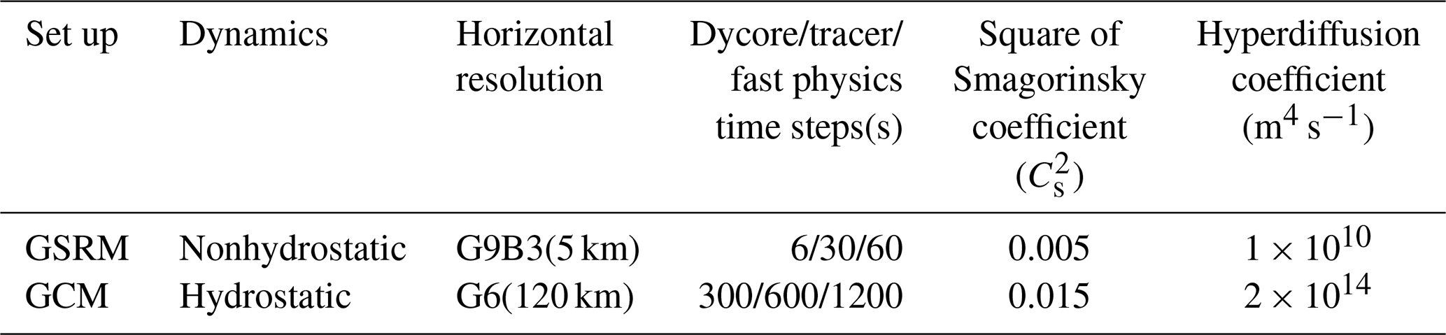
The GCM configuration follows the setup described in Zhang et al. (2021), using the hydrostatic dynamical core coupled with the conventional parameterization suite (CPS), and the cumulus parameterization is enabled. All other physics schemes – including microphysics, boundary layer, radiation, surface layer, and land surface model – are identical between the GSRM and GCM configurations, thereby maximizing consistency. Table 1 compares some other details of these two configurations.

Table 1 The GSRM and GCM configurations of GRIST for this study.

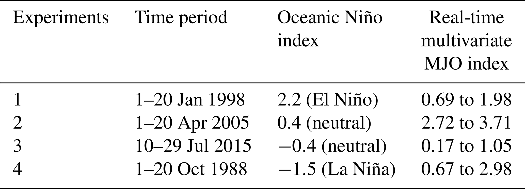
To enhance the representativeness of the training data, we select four 20 d periods (Table 2) that span different seasons and capture key phases of the El Niño–Southern Oscillation (ENSO) and Madden–Julian Oscillation (MJO). These periods collectively ensure comprehensive seasonal coverage – January (boreal winter), April (boreal spring), July (boreal summer), and October (boreal autumn) – and systematically represent the dominant ENSO–MJO interaction regimes that drive climate variability. Because online evaluation is the ultimate goal, offline evaluation serves as an important, albeit intermediate, step. A 7:1 ratio was used to divide the dataset into training and validation sets. For each day, 12.5 % of the time points were randomly allocated to the validation set, and the remaining 87.5 % were used for training. Moreover, we have further conducted a fully independent 10 d GSRM experiment (date: 14–23 July 2008) for final validation to assess the model's out-of-sample performance (Fig. 2). The current choice of 80 d reflects a practical limitation due to resource constraints, but it already allows essential atmospheric physical processes to be effectively learned by the AI model using a limited set of time windows. That said, increasing the number of training samples may further enhance the performance of the MPS.

Table 2 Selected time periods and climate characteristics.

2.2 Coarse graining and data preprocessing

We extract multiscale flow interactions in the GSRM using a thermodynamic framework following Yanai et al. (1973), in which the apparent heat source (Q₁) and apparent moisture sink (Q₂) serve as mathematical representations of these interactions. These quantities are derived from coarse-grained GSRM data at 0.25° resolution using the residual method (e.g., Zhang and Chen, 2016). The coarse-graining operation is interpreted here as (implicit) filtering, which itself warrants further investigation. We adopt conservative remapping, which has a strong effect of smoothing small-scale features (Chen et al., 2026). To apply the residual method, we use these coarse-grained states to represent scales larger than the native GSRM grid scale. Specifically, we compute the local time tendency, grid-scale advective tendencies, and the “ωα” term, where ω is the pressure-based vertical velocity and α is specific volume (Fig. 1). The gradient operator for evaluating the advective tendencies is achieved via the center difference method. These terms are then used to derive diabatic heating and drying rates, which can be interpreted as “sub-grid” tendencies relative to the coarse-grained scale. A key consideration is that the effective timescale of “parameterized tendencies” must be consistent with the timestep of the target coarse-resolution GCM. If this timescale is too long or too short, the estimated diabatic heating may become inappropriate, as Q₁ and Q₂ are highly discontinuous in time. This issue is discussed further in Sect. 2.4 in the context of temporal-resolution alignment.

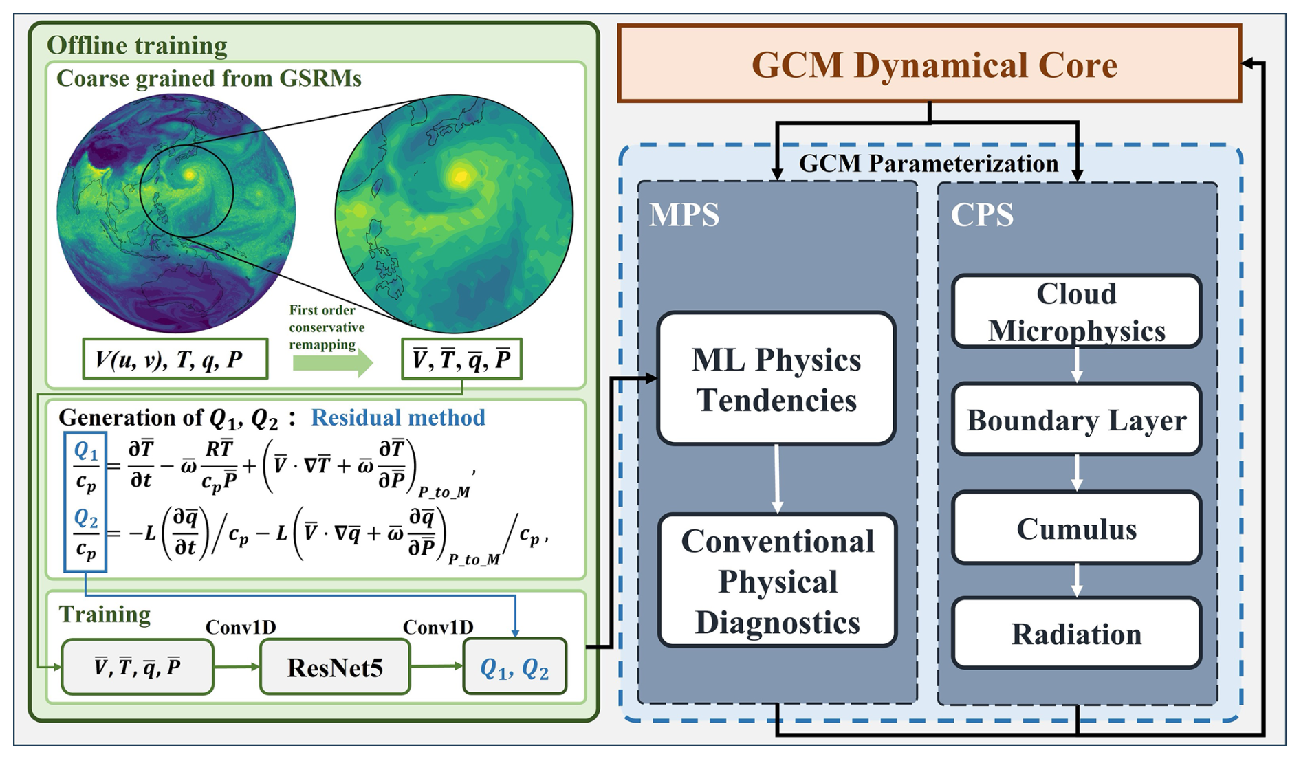
Figure 1 The workflow of offline training of MPS (Machine-Learning Physics Suite; Sect. 2.1–2.3) and online simulation of the GCM with ML-physics (Sect. 2.5). In the equations, T represents temperature, q specific humidity, V horizontal wind components (zonal u and meridional v), ω vertical velocity, R the gas constant for dry air, P the atmospheric pressure at all vertical levels, c_p the specific heat at constant pressure, and L latent heat of evaporation or condensation. The notation $\stackrel{\mathrm{‾}}{(•)}$ represents the horizontal coarse-graining operator, from 5 to 30 km in this study. The subscript P_to_M represents the conversion from pressure coordinate to the model level, after the calculation of advection terms on the pressure level.

While this study coarse-grained GSRM data to a fixed resolution, the residual method is inherently adaptable across resolutions. In principle, it can bridge models at arbitrarily high resolution to a range of target coarse scales. Establishing a robust correspondence between GSRMs and GCMs would not only enable GCMs to emulate selected behaviors of GSRMs but also create opportunities for a more unified representation of atmospheric processes within a single modeling framework. Such a framework could improve both theoretical understanding and predictive skill across scales. This architecture-agnostic framework offers two advantages: (i) ability to enable the transfer of scale interactions represented in GSRMs to a target GCM resolution, and (ii) interoperability with the broader modeling community using standard pressure-level atmospheric variables (i.e., less model dependent). Several key design choices are further highlighted below.

Choice of Large-Scale Variables: some preliminary tests identified the optimal set of input features to include temperature (T), specific humidity or mixing ratio (q), horizontal wind components (U and V), and surface pressure (P). Although the inclusion of vertical velocity (ω) is theoretically advantageous, it was found to introduce numerical instabilities in regions with complex topography – a result consistent with previous studies (Clark et al., 2022, Rasp et al., 2018; Watt-Meyer et al., 2024). All prognostic variables were normalized using min–max scaling, based on their extrema within the 80 d training dataset.

Vertical coordinate alignment: for machine learning training, it is desirable to use the model's native hybrid coordinate, which avoids topographic distortion during runtime. Calculating $Q_{\mathrm{1}}/Q_{\mathrm{2}}$ in the residual method requires first obtaining the advection tendencies. However, directly computing advection tendencies offline on the hybrid vertical coordinate is inaccurate because the generalized vertical velocity cannot be reliably reconstructed from coarse-grained data. It would require the generalized vertical velocity to be explicitly saved during the online integration, which is currently not available. More importantly, we prefer to confine our training workflow to standardized pressure-level variables as inputs, ensuring that the workflow has the potential to be consistently applicable to non-GRIST GSRM datasets.

To reconcile this discrepancy, we implement a two-step procedure. In Step I, GSRM variables on the hybrid model coordinate are interpolated to pressure levels for the sole purpose of computing advection tendencies. In Step II, the resulting advection tendencies are interpolated back to the model's hybrid coordinate, where Q₁ and Q₂ are then derived. Ultimately, all training inputs (U, V, T, q, P) and outputs (Q₁ and Q₂) are defined on the model's hybrid vertical coordinate, ensuring compatibility with the runtime model structure while preserving physical accuracy in the derivation process.

Temporal resolution alignment: to enhance temporal resolution, we applied linear interpolation to convert hourly coarsened GSRM model outputs into 20 min interval data, effectively tripling the temporal sampling frequency. This refinement is crucial for improving stability and accuracy of online model integration, as it increases the time samples and better aligns the temporal characteristics of the training data with the timestep of the target GCM (see Sect. 2.4).

2.3 Training the MPS

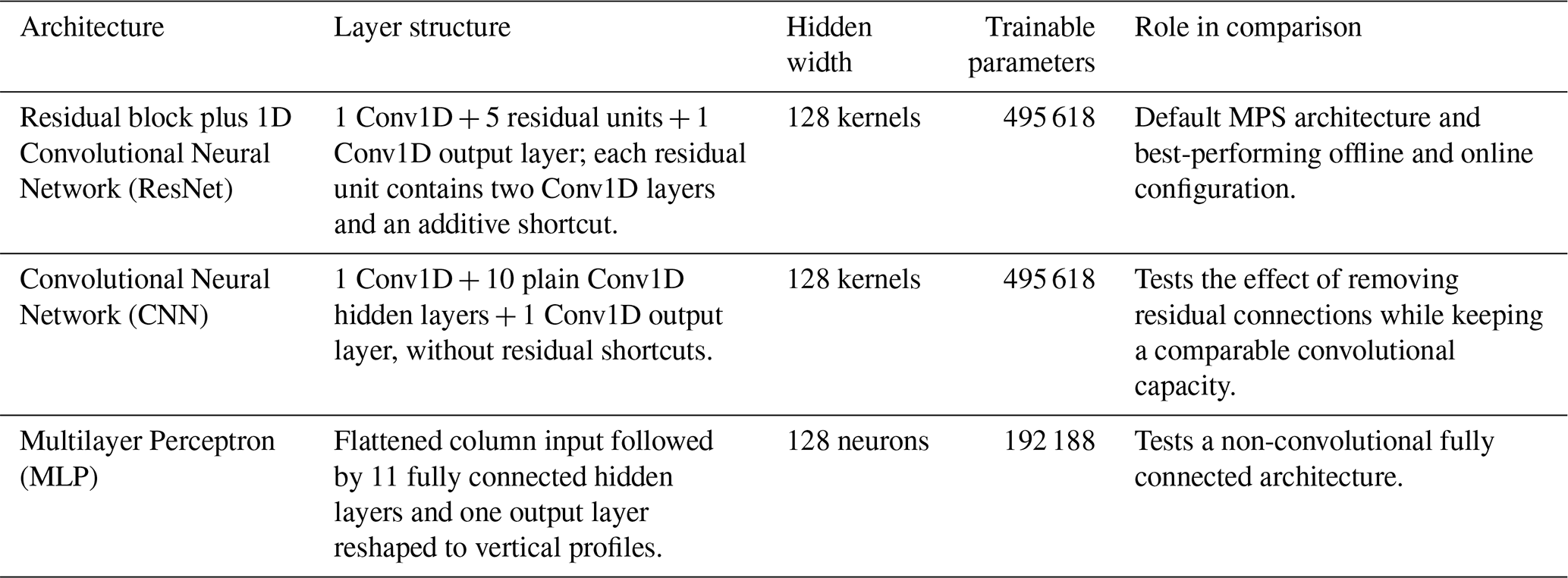
We examined three neural networks (Table 3). All of them share the same input variables, output variables, preprocessing procedure, loss function, optimizer, and online coupling interface, so the comparison isolates the effect of network architecture as much as possible. The input has 5 channels and 30 vertical levels, the output has 2 channels and 30 vertical levels, and the hidden width is 128. The ResNet consists of one initial 1D convolutional layer, five residual units, and one output convolutional layer, with each residual unit comprising two 1D convolutional layers plus an element-wise shortcut addition. The plain CNN retains the same number of convolutional weight layers but omits the residual shortcuts. The MLP consists of 11 fully connected hidden layers applied to the flattened vertical column, followed by a single output layer. The trainable parameter counts are 495 618 for ResNet, 495 618 for CNN, and 192 188 for MLP. ResNet and CNN have identical parameter counts because the residual shortcut is an Add operation and introduces no trainable parameters.

Table 3 The three networks studied and their specific setup.

The MPS leverages residual neural network architecture (ResNet) by default, with tailored modifications for atmospheric column physics. One-dimensional convolutional layers have the potential to explicitly resolve vertical couplings in temperature and humidity profiles, particularly during deep convective events where multi-level interactions dominate subgrid energy transfer. To balance representational capacity with computational efficiency, the network employs five optimized residual units (called ResNet5; Fig. 1) – a depth empirically determined to preserve most validation accuracy of deeper architectures while saving a lot of training time and resources. We used the Adam optimizer with a constant learning rate of $\mathrm{3}\times {\mathrm{10}}^{-\mathrm{4}}$ and a weight decay of 10⁻⁶. The mean absolute error (MAE) loss was selected over the mean squared error (MSE) loss as the loss function, as it demonstrated superior performance with lower biases on validation sets during initial training phases.

To optimize computational efficiency while maintaining global representativeness, we implemented a stratified spatiotemporal sampling strategy. Each temporal snapshot (20 min interval) extracts 64 800 grid columns distributed across key climate regimes: 50 % from tropical latitudes (30° S–30° N) where convective processes dominate, 30 % from mid-latitudes (60–30° S and 30–60° N) capturing baroclinic eddy activity, and 20 % from polar regions (90–60° S and 60–90° N) resolving radiative-polar amplification feedbacks. This geographic weighting generates 373,248,000 training samples (80 d × 24 h × 3 samples per hour × 64 800 columns). The network was trained for 100 epochs with a batch size of 1024 and early stopping (patience = 5 epochs, δval_loss < 0.5%) to ensure full data utilization without overfitting.

Rigorous offline evaluation is important for transitioning ML physics into an operational tool. We quantify emulation fidelity through two complementary metrics: (i) total mean squared error on validation sets (MSE < 1 × 10⁻⁴) and (ii) vertical-latitude cross-sections of the coefficient of determination (R²>0.3 across most of tropical and midlatitude tropospheric grid points; Fig. 2a and b), which collectively verify process-level skill in moisture–convection coupling. Networks satisfying both thresholds proceeded to online testing. This dual-criterion screening prevents numerically stable but physically implausible models from entering computationally intensive online integration phases. In the offline evaluation, ResNet outperforms CNN and MLP (Fig. 2c and d). Thus, ResNet is used as default unless otherwise mentioned.

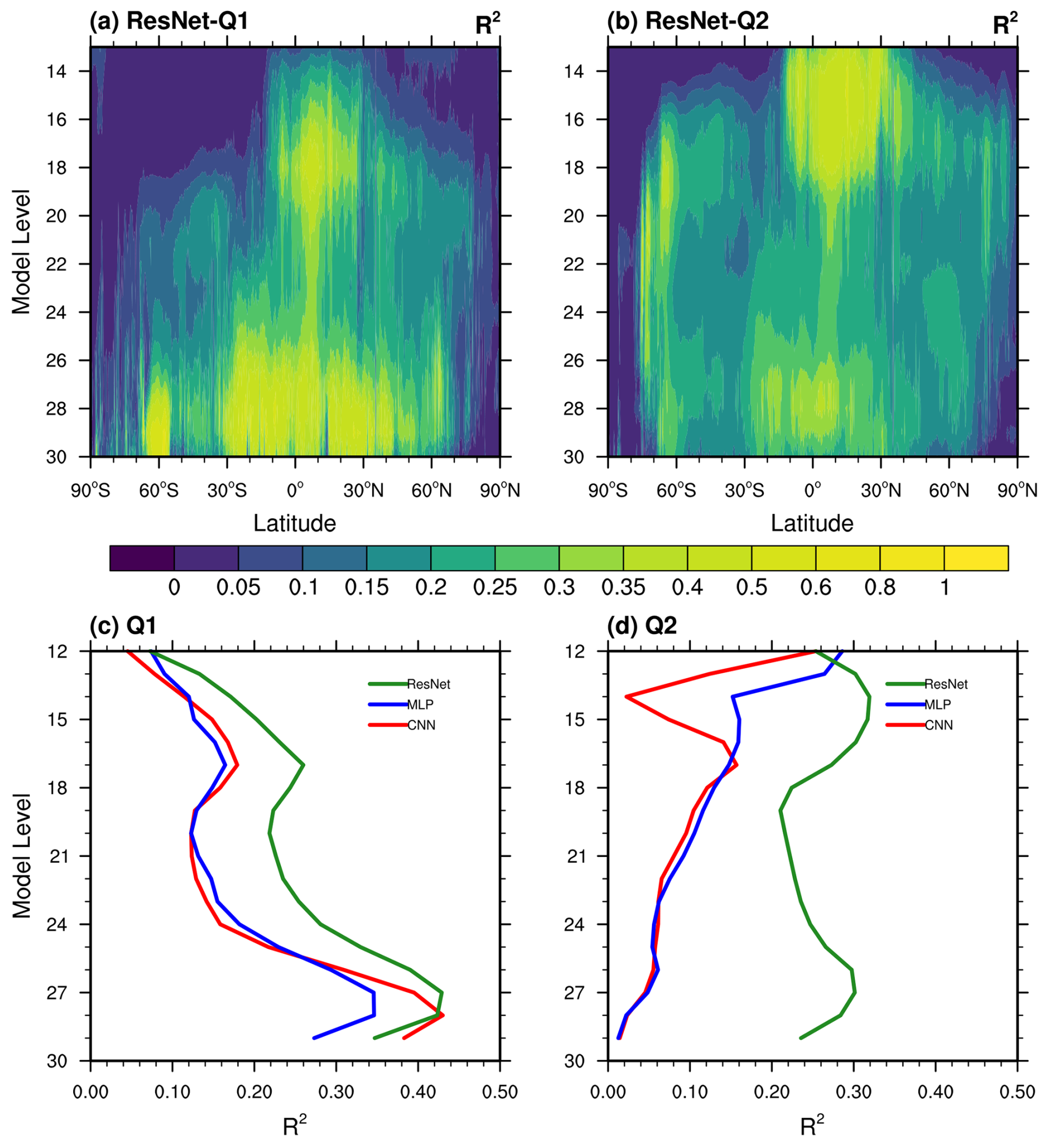
Figure 2 Offline skill of the coefficient of determination (R²) for (a) Q₁ and (b) Q₂, as functions of latitude and model level. The neural network is ResNet. Spatially averaged (30° S–30° N, 180° W–180° E) R² for (c) Q₁ and (d) Q₂, using three networks (ResNet, CNN and MLP). This validation is based on an independent GSRM simulation dataset out of the 80 d simulation samples.

Table 4 The optimal MPS experimental results of each setup. The bold format indicates improvements due to each sensitivity test.

Superior offline performance alone does not guarantee online stability, as the effects due to physics–dynamics coupling cannot be fully evaluated offline. To address this, we first shortlisted networks that met our predefined offline criteria, then we used them for online testing. The final selection of our optimal MPS is based on a dual evaluation: satisfying offline performance benchmarks (MSE < 1 × 10⁻⁴ and R²>0.3 on validation sets) and demonstrating stability in online integration, which must maintain stable online integration for more than 3 months. For the NNs that met the above criteria, we continued the online integrations to assess their long-term stability. Among the eight NNs – all sharing the same ResNet architecture but initialized with different random seeds – two remained stable for over 6 years, while the rest eventually developed numerical instabilities. We selected the better-performing model between them as the optimal MPS, based on its lower RMSE values for online variables such as precipitation (see Table 4).

2.4 Importance of balanced spatiotemporal sampling and temporal resolution alignment

During model development, we identified two key factors that significantly improve the stability and accuracy of the MPS. The first is achieving a more balanced spatiotemporal sample. Initial experiments using the full spatial samples (1440×720 grid columns per timestep) combined with coarse temporal sampling (hourly data) led to numerical instabilities during online integration. This instability stemmed from an extreme space–time sampling ratio, which caused the neural network to overfit spatial patterns while failing to adequately learn temporal evolution. To address this issue, we adopted a stratified spatiotemporal subsampling approach: at each timestep, only 64 800 geographically distributed columns were randomly selected, and the temporal resolution was increased to 20 min intervals via linear interpolation. This strategy balanced spatial and temporal dimensionality while effectively increasing the number of training samples, encouraging the network to focus on both the time evolution of atmospheric processes and static spatial features.

The second key aspect is aligning the temporal resolution of the data with the model's integration timestep. As noted earlier, we refined the temporal resolution of the large-scale variables by linearly interpolating hourly data to 20 min intervals prior to computing Q₁ and Q₂ tendencies. This refinement offers two primary benefits. First, the use of linear interpolation is justified for large-scale state variables, which typically evolve quasi-linearly over sub-hourly timescales (Δt<1 h). However, this assumption does not hold for Q₁ and Q₂, which exhibit stronger spatiotemporal nonlinearity. To make the effective time scale of Q₁ and Q₂ closer to the target timestep of the GCM, using linear interpolation of the large-scale variables is a practical choice. Second, doing so augments the dataset by a factor of three, providing a regularization effect. Although the interpolated data are correlated, this can partly improve model stability and generalization (Bishop, 1995), because Q₁ and Q₂ support a more aligned time scale and have more samples. As such, performing interpolation only on the input variables – rather than generating full 20 min GSRM outputs – achieves a 2/3 data compression ratio compared to storing the full-resolution dataset. Linear interpolation is not the only means of generating more data; one may alternatively choose to directly sample the model state at finer, aligned timesteps, but this is more expensive. While temporal resolution alignment is the key, our results demonstrate that the linear interpolation of large-scale state variables serves as an effective economical alternative to finely sampled model output.

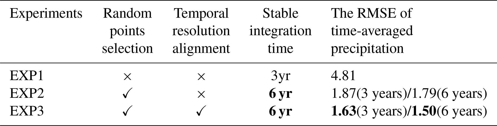
Altogether, these two methods enhance the stability and the accuracy of the simulations. The systematic evaluation of training strategies (Table 4) highlights the critical role of spatiotemporal data optimization in governing model performance. In the baseline experiment (EXP1), which employed neither spatial subsampling nor temporal refinement, the model maintained stability for only 3 years. Introducing spatial subsampling alone (EXP2) extended stable integration to 6 years. Further incorporating 20 min temporal interpolation in EXP3 – i.e., full spatiotemporal optimization – maintained 6-year stability while substantially reducing the tropical precipitation RMSE by 66 % (1.63 mm d⁻¹ vs. 4.81 mm d⁻¹ in EXP1). Compared to EXP2, EXP3 yielded a 16 % reduction in 6-year mean precipitation RMSE (1.50 mm d⁻¹ vs. 1.79 mm d⁻¹), demonstrating the additive benefit of temporal refinement beyond spatial subsampling alone. This underscores that careful data curation, without modifications to the AI-model architecture, can effectively address key challenges in ML–physics integration.

2.5 Online GCM simulation workflow with the MPS

The ML-physics-hybrid GCM builds upon the GRIST framework, with the control experiment (CPS) replicating the configuration described in Zhang et al. (2021) (Table 1, GRIST-CPS). To interface the Fortran-based GRIST model code with the PyTorch-formatted MPS, we implemented bidirectional coupling through the Ftorch library – a framework enabling real-time tensor exchange between the dynamical core and pretrained neural networks while maintaining operational efficiency.

The online implementation (Fig. 1, right panel) adopts a modular architecture, in which the GRIST-GCM dynamical core iteratively transfers atmospheric state tensors to the MPS. The MPS, interfaced via Ftorch, returns Q₁ and Q₂ tendencies, while legacy CPS diagnostic modules – such as radiation and land-surface coupling – remain unmodified. By restricting replacements to the physical tendency generation components and preserving the native diagnostic workflow, the framework mirrors the CPS substitutions and ensures full backward compatibility. The replaced CPS components include tendencies from the cumulus parameterization, cloud microphysics, boundary layer scheme, and radiative transfer. The radiation module – the most computationally expensive element in the CPS – is still activated to generate surface fluxes for the land surface and may require dedicated training in the future. The surface layer and land surface models are also retained in their original form, consistent with standard CPS configurations. Surface precipitation flux (Prec; unit: kg m⁻² s⁻¹) is diagnosed by the MPS via vertically integrated moisture tendency equation plus the evaporation flux (Evap), calculated using: $\mathrm{Prec}=-\frac{\mathrm{1}}{g}\int (Q_{\mathrm{2}}/L)\mathrm{d}p+\mathrm{Evap}$. The evaporation term is included solely for diagnostic purposes; the precipitation input provided to the land surface model excludes this term, as a tuning procedure.

Due to the MPS's coarser vertical resolution in the lower troposphere (Δz exceeding 200 m below 850 hPa), we retain CPS-derived temperature tendencies (Q₁) in the lowest four model levels and moisture tendencies (Q₂) in the lowest two model levels. This selective preservation, validated through sensitivity experiments, serves as a stability-enhancing mechanism, the present MPS without this configuration will crash after running for a few days. Meanwhile, as in prior studies (Brenowitz and Bretherton, 2019; Clark et al., 2022; Watt-Meyer et al., 2024), we apply vertical truncation of the MPS-predicted $Q_{\mathrm{1}}/Q_{\mathrm{2}}$ tendencies above 300 hPa, effectively excluding the top 12 model layers from machine-learned physics. This leaves room for future improvement. Because the dominant portion of the total physical tendencies is supplied by the ML-based physics, the conventional parameterizations, although still active during the model integration for diagnostic purposes, passively respond to the prognosed grid-scale states but exert little direct influence on them, except at the specific levels as noted above.

This hybrid replacement strategy demonstrates that partial physics–ML integration can achieve climate fidelity comparable to a full replacement, while mitigating numerical instability. Furthermore, when extended to higher resolutions, it reduced computational costs by over 30 % with a similar configuration (Duan et al., 2025) when optimizations have been carried out. This is attributed to the more optimizable computational structures of ML models (convolution, matrix multiplication), which are clearly difficult to achieve in conventional schemes.

3 Results

3.1 Real-world climate simulations

Two 6-year AMIP-style simulations (2001–2006) were conducted at 120 km horizontal resolution: a control experiment with the CPS and an ML-enhanced counterpart with the MPS. We evaluate the zonal-mean vertical structures of long-term mean temperature (T) and specific humidity (q), which are directly affected by the MPS through Q₁ and Q₂, as well as zonal wind (U), which reflects dynamically constrained momentum redistribution. ERA5 reanalysis data (Hersbach et al., 2020) serve as the observational benchmark, with all model outputs regridded to 1°×1° resolution using conservative remapping.

Figure 3 demonstrates close alignment between GRIST-MPS and GRIST-CPS in simulating zonal-mean vertical structures. Both models exhibit temperature deviations (shading) within ±5 K from ERA5 reanalysis, demonstrating consistent cold biases in the polar lower stratosphere and warm biases in the tropical upper troposphere. Specific humidity profiles (black contours) display nearly identical vertical distributions between configurations. The structure of the zonal wind (U) forms a wedge-like structure with the humidity, showing little difference in midlatitude jet core positions.

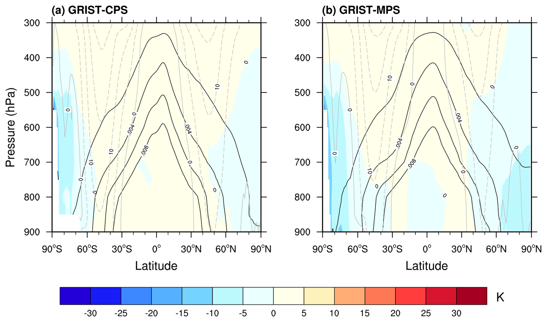
Figure 3 (a) Latitude–pressure cross section of the time averaged zonal mean temperature differences (shaded), climatology specific humidity (black lines) and climatology zonal winds (gray lines) with GRIST-CPS. (b) As in (a) but for GRIST-MPS simulation. The simulation period for all of the models was from 2001 to 2006.

Precipitation is evaluated against the Global Precipitation Measurement (GPM) Product (Huffman et al., 2019). Both configurations realistically capture the boreal summer (June–July–August; JJA) precipitation dipole – the Intertropical Convergence Zone (ITCZ, 0–15° N) and South Pacific Convergence Zone (SPCZ, 5–15° S) with maximum rates exceeding 12 mm d⁻¹ over the Bay of Bengal and western Pacific warm pool (Fig. 4a–c).

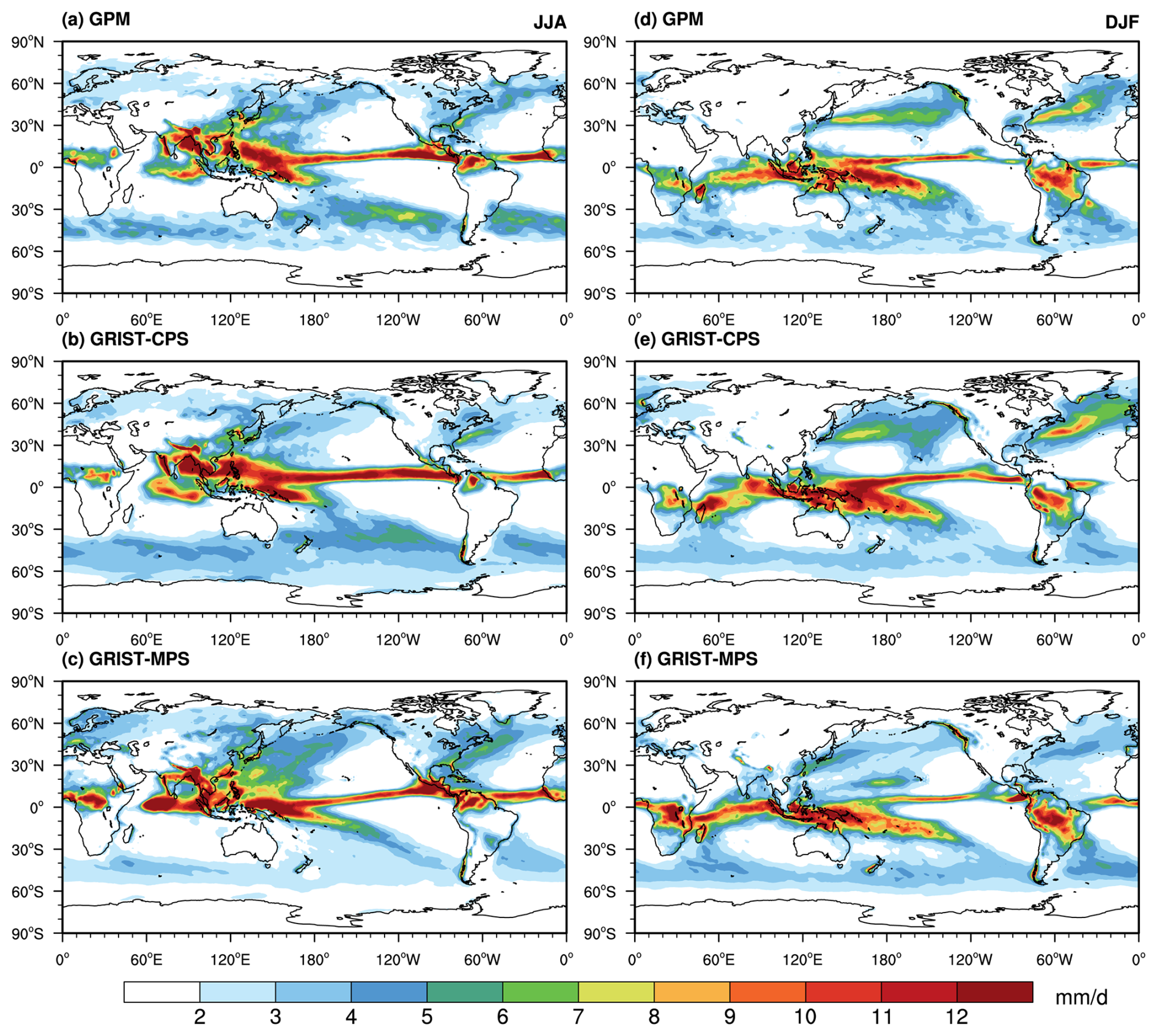
Figure 4 The mean precipitation rate (unit: mm d⁻¹) averaged from 2001 to 2006 for June–July–August (a–c) and December–January–February (d–f) by (a, d) GPM, (b, e) GRIST-CPS, and (c, f) GRIST-MPS.

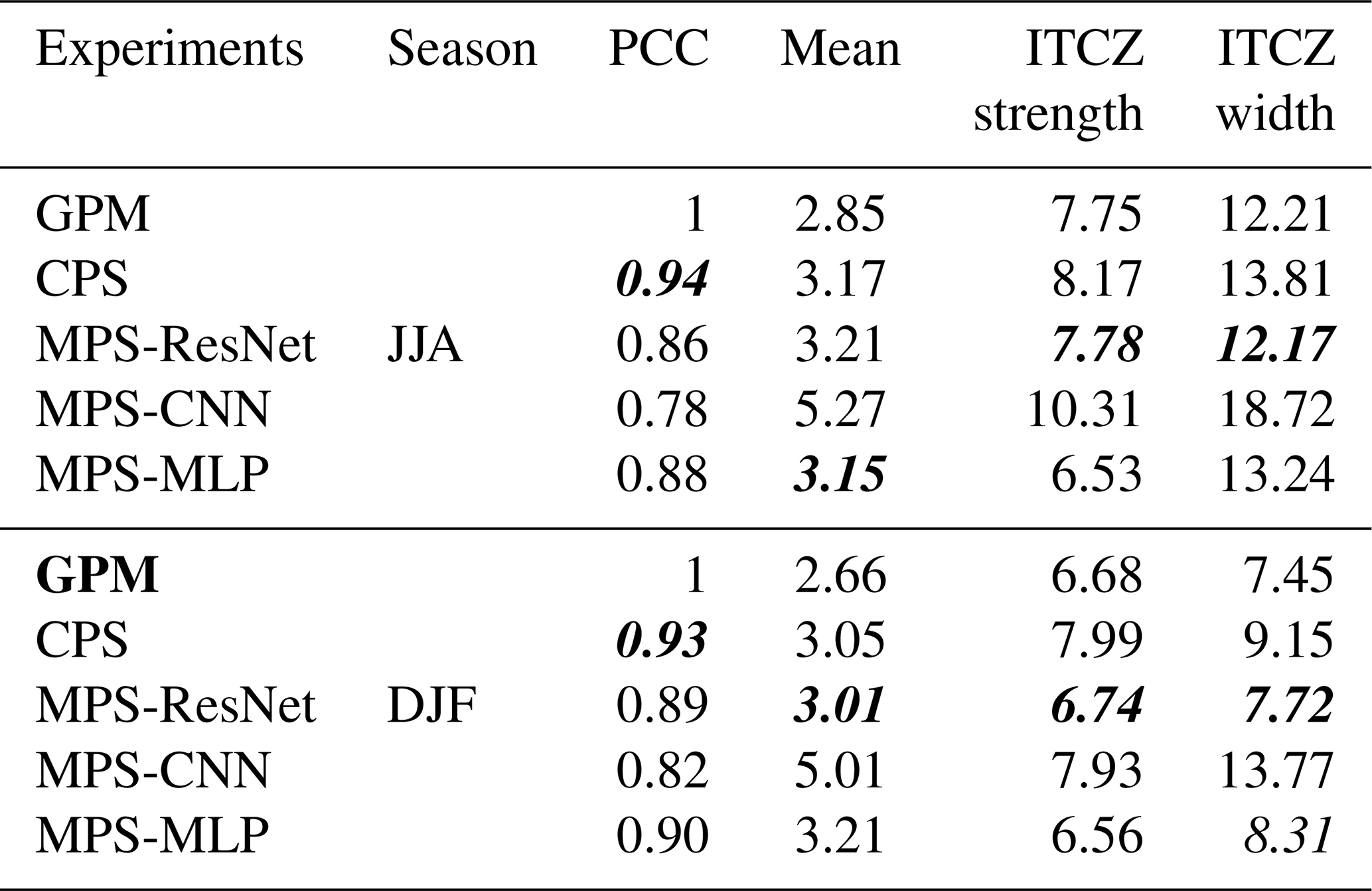
During JJA months (Table 5), GRIST-MPS produces a more realistic ITCZ than GRIST-CPS in terms of both strength and width. Following established conventions, we quantify the width of the ITCZ as the latitudinal distance between its northern and southern boundaries, applying a 5-point smoother to the data prior to calculation (Wodzicki and Rapp, 2016). The northern (southern) boundary is identified by moving equatorward from higher latitudes and locating the first grid cell where the precipitation in the adjacent grid cell to the north (south) falls below 2.5 mm d⁻¹. The strength of the ITCZ is defined as the area-weighted mean precipitation within the region bounded by these northern and southern boundaries (Wang et al., 2023). The MPS accurately captures the ITCZ strength (7.78 mm d⁻¹), closely matching the GPM estimate (7.75 mm d⁻¹). By contrast, the CPS produces an excessively strong (8.17 mm d⁻¹) and overly broad (13.81°) rain band, compared with the observed width of 12.21° and the MPS width of 12.17°.

Table 5 The performance metrics from the 6-year simulations for each experiment during summer (June–July–August, JJA) and winter (December–January–February, DJF). The metrics include the spatial pattern correlation (PCC), global-mean precipitation (mm d⁻¹), ITCZ strength (mm d⁻¹), and ITCZ width (degrees). Values in bold and italic indicate the closest match to the observations.

Extratropical performance remains comparable, with both models capturing most of observed midlatitude storm-track variance (55–65° N). The MPS slightly underestimates precipitation over the southern oceans (30–70° S) at 2.19 mm d⁻¹ against the observed 2.67 mm d⁻¹, whereas the CPS overestimates it (3.25 mm d⁻¹), with the bias extending to 70° S.

During boreal winter (December–January–February; DJF), GPM observations reveal a meridionally contracted state of tropical rainbands and intensified midlatitude storm-track precipitation (45–60° N, Fig. 4d). Both configurations capture this seasonal transition (Fig. 4e and f), with GRIST-MPS demonstrating enhanced fidelity over the equatorial Pacific (20° S–20° N, 120° E–90° W) and South America (30–0° , 80–40° W) through a 4 % RMSE reduction (1.96 mm d⁻¹ vs. 2.04 mm d⁻¹). In particular, over the South American region, the spatial correlation coefficient of MPS precipitation (0.95) exceeds that of the CPS (0.93).

Meanwhile, some remaining biases persist in GRIST-MPS: compared to GRIST-CPS, its global spatial pattern correlation coefficient is marginally lower (PCC: MPS: 0.86 vs. CPS: 0.94) in summer. It exhibits dry biases over the northern and southern subtropical oceans in winter, alongside a consistent moist bias over Africa in both seasons. In addition, GRIST-MPS shows a 15 %–20 % overestimation of summer tropical Indian Ocean rainfall (10° S–10° N, 65–95° E), a 4–6 mm d⁻¹ overestimation over the northern equatorial Pacific (0–20° N, 120° E–90° W), and a systematic 1–3 mm d⁻¹ underestimation of precipitation over the Southern Ocean (50–60° S) and the Maritime Continent (5° S–5° N, 95–150° E) across seasons.

Both configurations accurately reproduce the observed seasonal migration of tropical precipitation maxima (Fig. 5), with boreal summer peaks centered near 5–10° N aligned with the northward-migrating ITCZ. However, systematic discrepancies emerge in the meridional range of precipitation representation: GRIST-CPS overestimates the central precipitation intensity, generating strengthened rainfall distributions of overactive convective initiation in cumulus parameterizations. GRIST-MPS shows a slight overestimation of the precipitation range throughout the seasonal cycle.

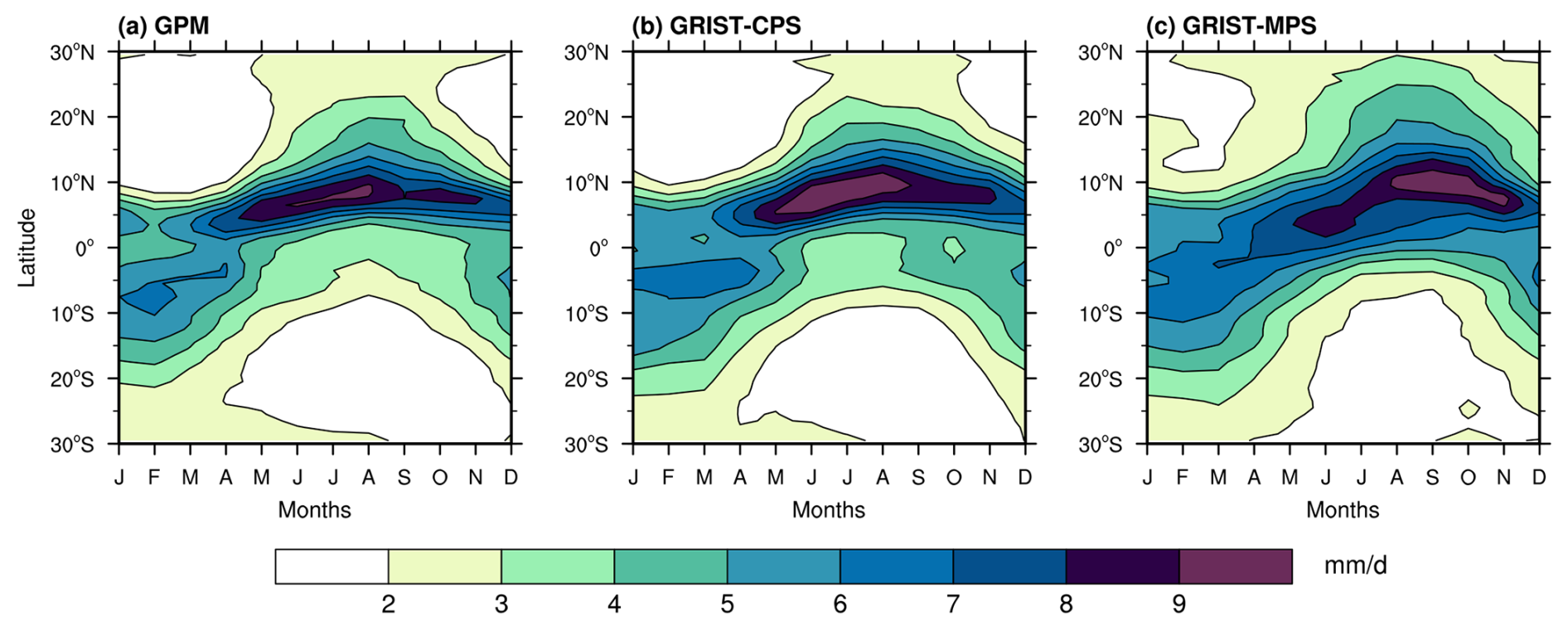
Figure 5 Seasonal evolution of tropical precipitation from 2001–2006 for observation from (a) GPM, (b) GRIST-CPS, and (c) GRIST-MPS (unit: mm d⁻¹).

To systematically assess the performance of GRIST-MPS in characterizing complex atmospheric systems, we employ the East Asian Monsoon as our case study. Our analysis utilizes an established East Asian monsoon index (EAMI) from prior studies as a benchmark metric (Zhu et al., 2005). The EAMI takes the influence of the annual cycle of the meridional and zonal sea-land thermal differences into account in the East Asia-Pacific region and reasonably describes the characteristics of the annual cycle of the transition between the East Asian winter and summer monsoons, which is defined as:

$$\begin{array}{}\text{(1)}& \begin{array}{rl}\mathrm{EAMI}& =\left(U_{\mathrm{850}\mathrm{hPa}}-U_{\mathrm{200}\mathrm{hPa}}\right){\ast }_{(\mathrm{100}\text{–}\mathrm{130}\mathit{°}\mathrm{E},\mathrm{0}\text{–}\mathrm{10}\mathit{°}\mathrm{N})}\\ & +\left({\mathrm{SLP}}_{\mathrm{160}\mathit{°}\mathrm{E}}-{\mathrm{SLP}}_{\mathrm{110}\mathit{°}\mathrm{E}}\right){\ast }_{\left(\mathrm{10}\text{–}\mathrm{50}\mathit{°}\mathrm{N}\right)}\end{array}\end{array}$$

where U represents area-averaged (100–130° E, 0–10° N) monthly mean zonal winds (dimensionless), SLP denotes averaged monthly sea level pressure (10–50° N) (dimensionless), and the asterisk (∗) operator indicates variable standardization through mean removal and unit-variance scaling ($X=(X-\mathit{\mu })/\mathit{\sigma })$, where X is the corresponding variable (U, SLP), where μ represents the mean of variable X and σ represents the standard deviation of variable X. This enables a quantitative assessment of the model's ability to capture both the seasonal and interannual variability characteristics of monsoon dynamics.

We computed the EAMI for monthly variables and derived its climatological seasonal cycle across a 6-year period (Fig. 6). Both GRIST-CPS and GRIST-MPS successfully replicate the observed seasonal monsoon phase, capturing the July maximum and February minimum. While GRIST-CPS simulations align closely with observations, GRIST-MPS exhibits a systematic bias: it overestimates monsoon intensity prior to July and underestimates it post-July. This indicates that GRIST-MPS could simulate the annual cycle of the East Asian monsoon, even though the training data only includes 80 d. This outcome strongly motivates a further refinement of MPS for extended climate applications.

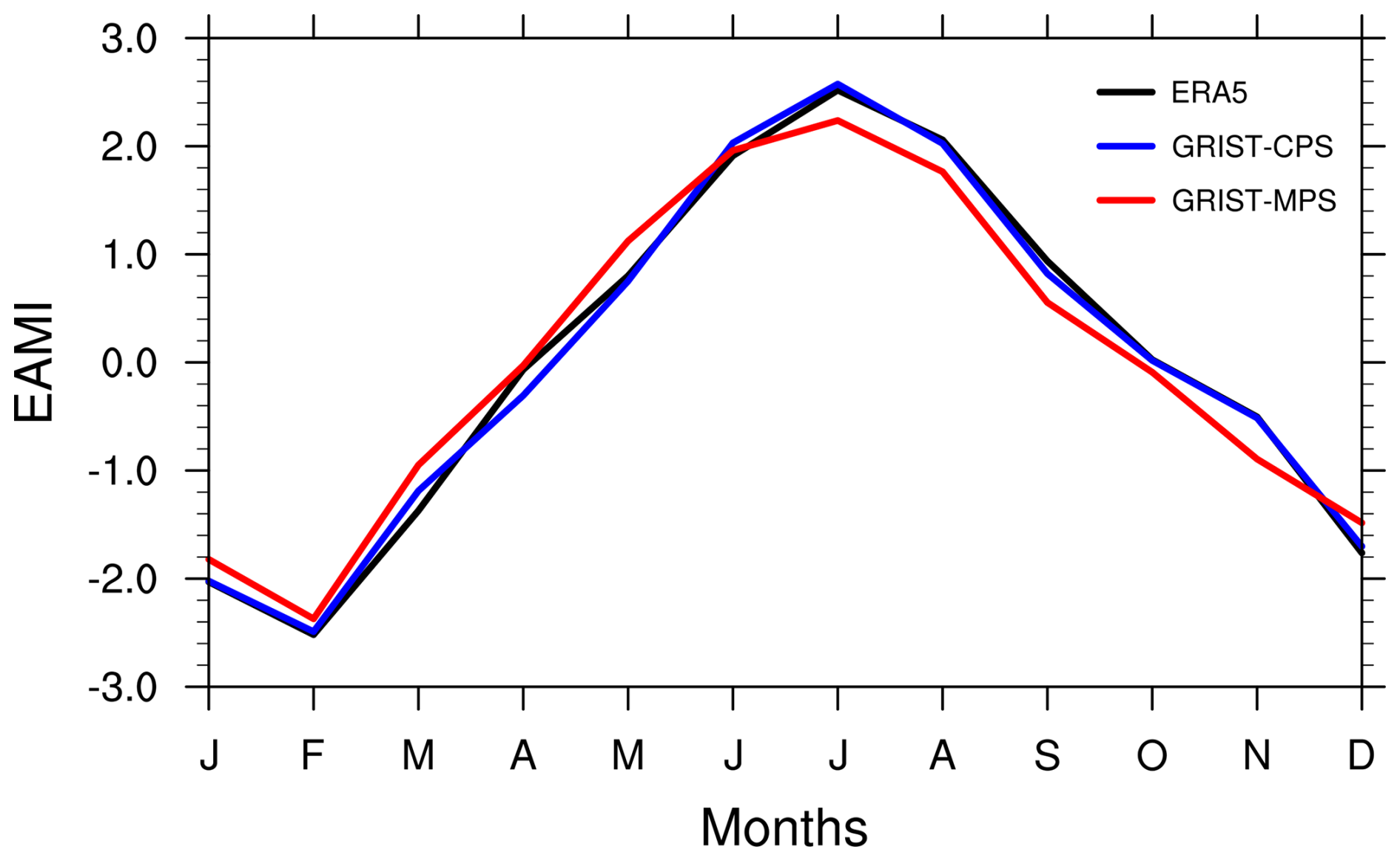
Figure 6 The East Asian Monsoon Index (EAMI) of ERA5 (black line), GRIST-CPS (blue line) and GRIST-MPS (red line).

The intensity–frequency distribution of precipitation reflects intrinsic model characteristics that remain stable over the course of a simulation. To assess whether the MPS faithfully captures the behavior of the GSRM, we conducted parallel experiments with the MPS and CPS using time periods aligned with the GSRM (i.e., the four cases listed in Table 2). Focusing on tropical precipitation (10° S–10° N), we categorize rainfall into four intensity ranges: light (0.1–10 mm d⁻¹), moderate (10–25 mm d⁻¹), heavy (25–50 mm d⁻¹), and extreme (>50 mm d⁻¹). As shown in Fig. 7a, relative to GRIST-CPS, the GSRM exhibits reduced total precipitation frequency and a lower frequency of light rainfall. GRIST-MPS consistently reproduces these features, with both total and light precipitation frequencies lower than in GRIST-CPS. Furthermore, comparing Fig. 7a and b reveals that both GRIST-CPS and GRIST-MPS display similar frequency characteristics in the GSRM-aligned experiments and the long-term free-run integrations, underscoring the robustness of these model behaviors.

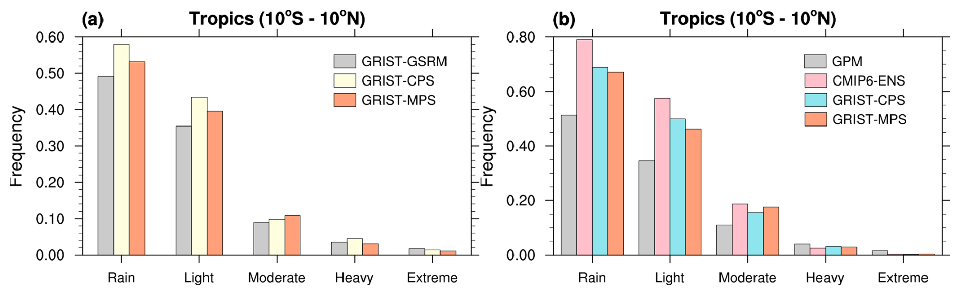
Figure 7 (a) The frequency distributions of tropical daily precipitation corresponding to the 80 d GSRM period, obtained from GSRM (gray boxes), GRIST-CPS (yellow boxes) and GRIST-MPS (orange boxes). (b) As in (a) but for precipitation frequency from 2001–2006, obtained from GPM (gray boxes), the ensemble mean of 11 CMIP6 models (CMIP6-ENS; pink boxes), GRIST-CPS (blue boxes) and GRIST-MPS (orange boxes).

Besides GPM observations, the ensemble-mean values of 11 CMIP6 models (CESM2, CESM2-WACCM, CMCC-CM2-SR5, E3SM-2-0, E3SM-2-0-NARRM, EC-Earth3, EC-Earth3-AerChem, GFDL-CM4, MRI-ESM2-0, SAM0-UNICON, TaiESM1; hereafter CMIP6-ENS) are included. Relative to GPM data, both CMIP6-ENS and GRIST-CPS overestimate total precipitation occurrence by 54 % and 34 %, respectively (Fig. 7b) – consistent with earlier documented biases (Fu et al., 2024). The MPS reduces this discrepancy to 31 %. It reduces light and heavy rain overprediction by 10 % and 5 %, respectively, while preserving observed extreme precipitation frequencies. This demonstrates that MPS effectively mitigates persistent precipitation distribution errors without compromising heavy-precipitation event statistics. Meanwhile, neither the CPS nor the MPS indicates a long-term artificial declining trend in precipitation (figure not shown).

3.2 A sensitivity analysis of different neural networks

Besides ResNet, we have also integrated two alternative neural network architectures – plain CNN without residual blocks and MLP without convolutional networks – to examine the sensitivity of online simulations to network architecture. The three networks are trained on identical datasets and preprocessing procedures. Switching networks during the GRIST-MPS runtime only needs to change the NN file which contains the weights and structures of each NN.

Figure 8 As in Fig. 3 but for (a) ResNet, (b) CNN and (c) MLP.

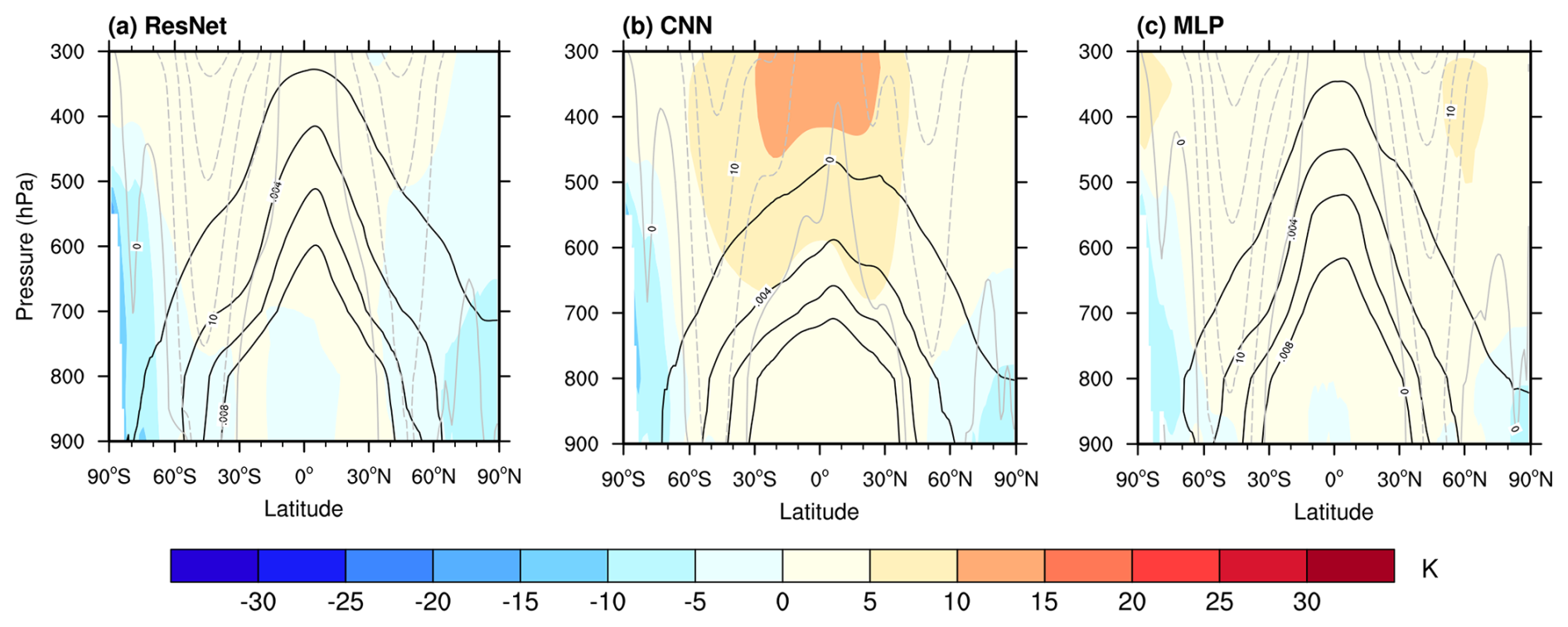
Comparative analysis of neural architecture reveals distinct thermodynamic fidelity characteristics (Fig. 8). ResNet architecture demonstrates superior temperature profile reconstruction, maintaining deviations < 5 K from ERA5 reanalysis throughout the troposphere. In contrast, CNN and MLP architectures exhibit systematic warm biases (5–10 K) between 300–600 hPa, while MLP exhibits warm biases at both the North and South poles. Humidity simulations further highlight architectural divergence: while CNN/MLP architectures compress moisture profiles toward lower altitudes (peaking at 850 hPa with about 50 % faster moisture decay rates above 500 hPa), ResNet and MLP preserve physically consistent specific humidity gradients up to 300 hPa, a capability enabling enhanced representation of upper-tropospheric moist processes. Wind field simulations demonstrate architectural invariance, indicating dynamical core constraints predominantly govern momentum balance regardless of physics parameterization. These findings indicate that neural network selection significantly influences thermodynamic fidelity, which is a critical design consideration for developing ML-based parameterizations. The results are consistent with the offline evaluation (Fig. 2), the ResNet produces the optimal outcome.

Neural architecture selection induces large discrepancies in precipitation simulations, particularly in tropical convective organization (Fig. 9). During boreal summer, the CNN architecture overestimates western Pacific and tropical Indian Ocean precipitation relative to observations, generating an excessively broad ITCZ with spurious drizzle artifacts across subtropical highs. The MLP produces weaker globally averaged precipitation than CNN (3.15 mm d⁻¹ vs. CNN's 5.27 mm d⁻¹, JJA) while maintaining comparable spatial PCC (0.88 vs. CNN's 0.78) to observations (Table 5).

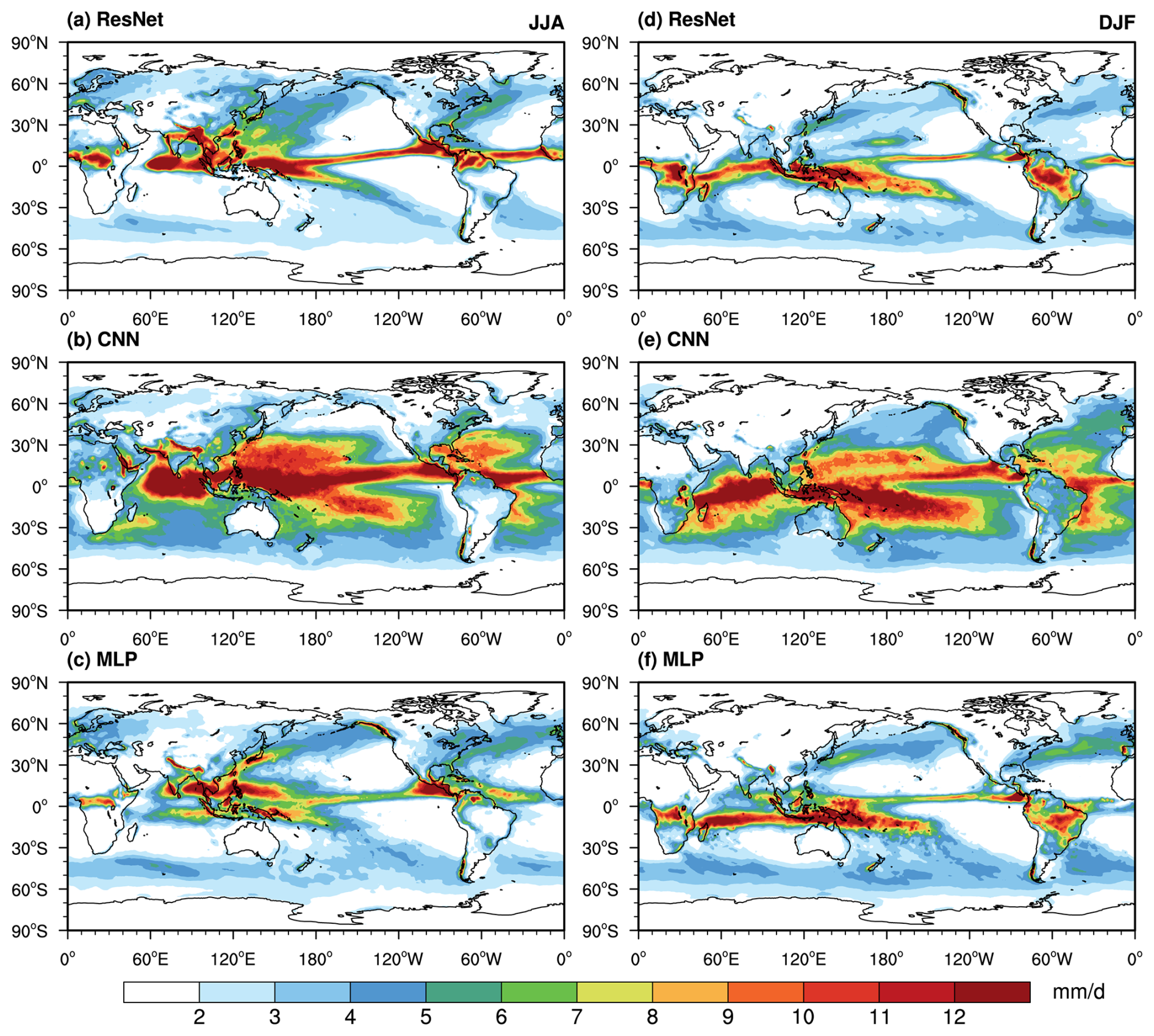
Figure 9 As in Fig. 4, but for (a) ResNet, (b) CNN, (c) MLP in JJA, (d–f) in DJF.

Winter simulations of CNN reveal pronounced biases: precipitation over the ITCZ and SPCZ exhibits large (more than 20 %) overestimation relative to observations. The MLP slightly underestimates the ITCZ strength in DJF by 2 %, but shows improved spatial pattern alignment with ResNet. The ResNet architecture consistently outperforms other configurations in maintaining a small deviation across seasons. These systematic discrepancies suggest that precipitation simulations are strongly influenced by architecture-dependent behavior, including differences in optimization, information propagation, and the subsequent amplification of tendency errors through online coupling. This underscores the critical need for architecture-specific uncertainty quantification in machine learning-driven climate modelling, as model design disparities directly shape predictive outcomes.

Figure 10 Same as in Fig. 5, but for (a) ResNet, (b) CNN, (c) MLP.

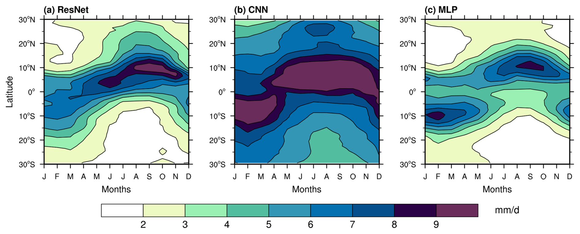
Seasonal precipitation migration patterns reveal distinct architectural sensitivities (Fig. 10). While all architectures capture fundamental north–south displacement of tropical precipitation maxima, CNN simulations exhibit greater meridional spread, consistent with documented overestimation of tropical precipitation (Fig. 9b and e). Conversely, MLP systematically underestimates peak precipitation intensities in summer, while overestimating the precipitation center of 10° S in winter by about 1 mm d⁻¹, a deficiency attributable to its limited capacity in resolving nonlinear moisture-convection feedback inherent to fully connected architectures. ResNet maintains the closest fidelity to observed seasonal progression (<5 % phase error in ITCZ migration timing).

The frequency-intensity distribution of precipitation (Fig. 11) reveals neural architectural influences on precipitation distribution characteristics: CNN more than doubled the frequency of light precipitation occurrence compared with conventional GCMs. Conversely, the MLP achieves the closest alignment with observed frequency distributions despite systematically underestimating heavy precipitation (>50 mm d⁻¹). The MLP shows better agreement in light-rain frequency despite its overall weaker precipitation intensity. This apparent paradox originates from the smoother and weaker $Q_{\mathrm{1}}/Q_{\mathrm{2}}$ responses produced by the MLP in the online simulations, which tend to suppress heavy precipitation while keeping the dominant light-rain category (1–10 mm d⁻¹) closer to observations. ResNet demonstrates intermediate performance.

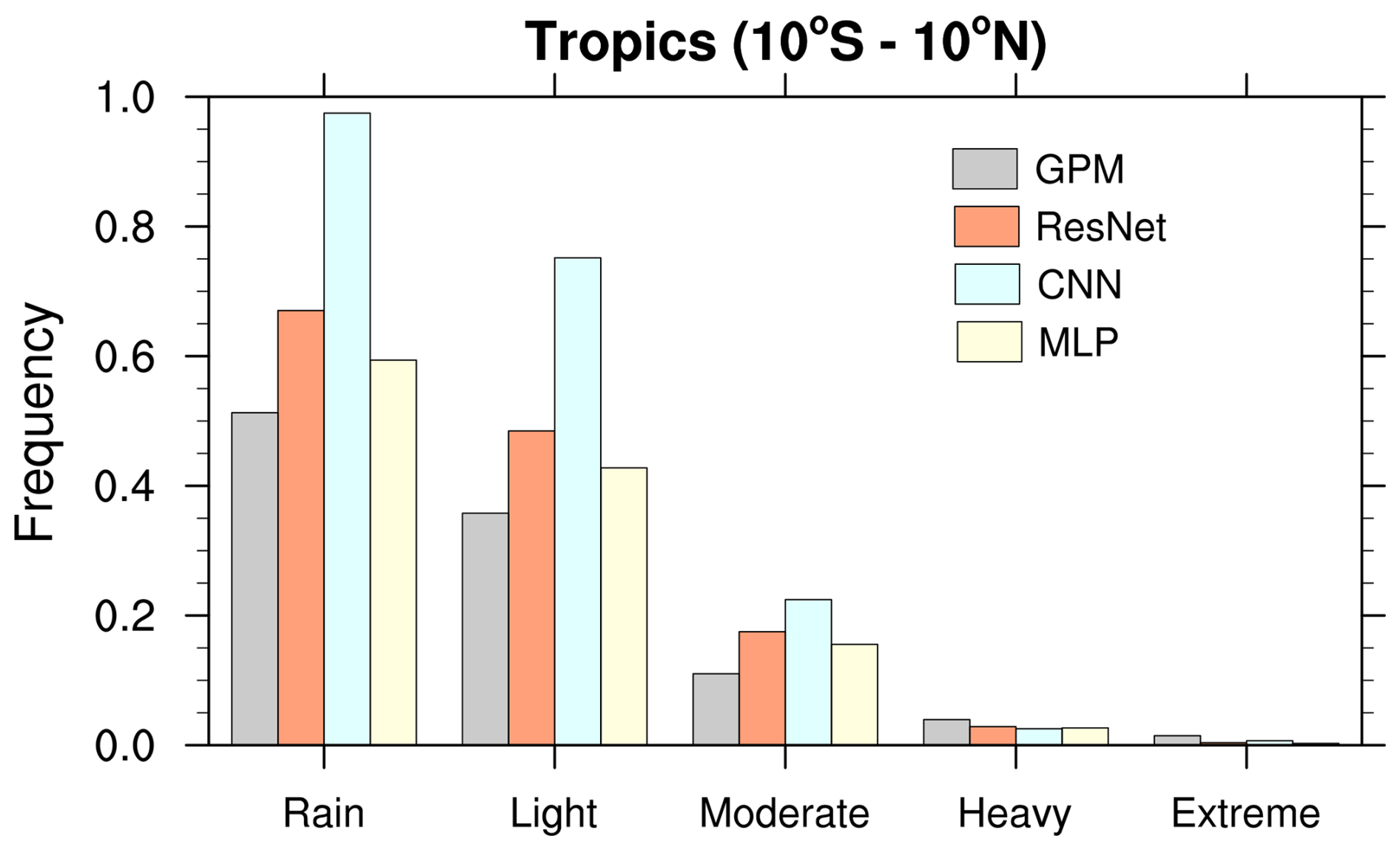
Figure 11 As in Fig. 7b but with CNN (blue bins) and MLP (yellow bins) added, and CMIP6-ENS omitted.

Meanwhile, we have also evaluated the deterministic prediction skill of GRIST-CPS and GRIST-MPS using short-term numerical weather prediction–type experiments (results provided in the Supplementary Material). For precipitation frequency, MPS still outperforms CPS; however, the deterministic skill – quantified by the anomaly correlation coefficient (ACC) for several prognostic fields – is lower than that of CPS, indicating room for improvement of large-scale forecast skills.

4 Summary and outlook

This study establishes a new ML-physics hybrid modeling framework through seamless integration of neural networks trained on high-resolution GSRM data into a GCM, achieving stable 6-year climate simulations with enhanced process-level fidelity. The major conclusions are summarized below.

Major achievement: the GRIST-MPS exhibits strong thermodynamic consistency, closely replicating ERA5 vertical profiles of temperature (T bias < 5 K) and specific humidity (q bias < 1.5 g kg⁻¹), while improving tropical precipitation primarily through improved representation of convective–diabatic processes. Key improvements include more accurate ITCZ strength and width, phase-aligned midlatitude storm tracks, and improved precipitation frequency, particularly the improved light rainfall frequency (0.1–10 mm d⁻¹). Crucially, the framework preserves long-term numerical stability and accuracy through architectural innovations and an optimized spatiotemporal sampling strategy, all embedded within a workflow built on standardized pressure-level input variables. These results demonstrate that ML–physics integration has the potential to overcome long-standing trade-offs in conventional parameterizations, offering a transformative pathway for next-generation climate modeling. Moreover, leveraging GSRM-driven learning to construct ML–physics hybrid GCMs offers distinct advantages: GSRMs inherently capture multiscale atmospheric interactions without imposing artificial scale separation, while allowing flexible resolution specifications. Furthermore, community-standardized GSRM datasets based on common state variables promote reproducibility and interoperability. We contend that this modeling paradigm paves the way toward unifying GSRM and GCM scales by harnessing the synergy of ML and high-fidelity data, offering a scalable and physically grounded foundation for future Earth system modeling.

Prospective Relevance: as a proof-of-concept study, this work provides a useful reference for future ML-based efforts by demonstrating that a column-based ML physics module, trained on GSRM multiscale modeling data over a limited time window, can produce realistic online free-running climate simulations and generalize to unseen periods. Beyond the choice of ML architecture, several strategies proved essential. First, spatial random sampling mitigated spatial overfitting arising from an imbalanced data distribution, improving both accuracy and stability. Second, interpolating the data from 1 h to 20 min resolution aligned the training data with the target model timestep, and partly increased the nominal number of training samples, thereby improving online stability and performance. Admittedly, the model still requires a small number of near-surface CPS tendencies (primarily for the boundary layer) to maintain online stability. This likely reflects a limitation of the coarse-grained dataset, which has a coarse vertical resolution in the lower troposphere (spacing > 200 m below 850 hPa). In addition, vertical eddy transport associated with boundary-layer turbulence may require higher-resolution training data to be represented effectively.

An important implication is that representing physics tendencies as residual terms of grid-scale variables is a promising route for diagnosing training targets for ML-based physics. This approach offers several potential advantages that merit further exploration. For example, a common high-resolution dataset can be incrementally coarse-grained to multiple coarser resolutions, enabling datasets at different resolutions to share consistent large-scale information. Moreover, the large-scale states can be further constrained (e.g., via short-period simulations and/or nudging), which may improve the quality of the diagnosed tendencies, and/or generate additional constraint-related tendencies that can be learned separately. However, unlike physics tendencies directly extracted from a host model, this reconstructed-tendency approach generally requires dedicated training strategies and careful coupling procedures to ensure stable and accurate online integration.

Remaining challenges: the current training is limited to only an 80 d GSRM dataset. Future extensions are expected to enhance model generalization and fidelity. As mentioned, one limitation of the present work is that the MPS-generated temperature and humidity tendencies replace the raw CPS tendencies almost, but not entirely (see Sect. 2.5). Meanwhile, another limitation of the present framework is the absence of momentum feedback in the ML architecture, which may lead to systematic biases in upper-tropospheric jet stream positioning (e.g., U bias > 5 m s⁻¹ at 200 hPa). Additionally, raw GSRM-derived multiscale interactions may require constraints. Despite these limitations, our results demonstrate that GSRM-trained, MPS-enhanced model physics can achieve simulation stability (over 6 years) and high physical fidelity (e.g., ITCZ positional refinement within 2° latitude). This provides a promising indication for scalable and physically consistent next-generation multiscale climate modeling paradigms.

Interdisciplinary implications: the ML–physics model introduces a novel computational framework that has interdisciplinary implications. The software framework presented can serve as a platform for testing ML-trained physics suites within hybrid AI-Physics GCMs. The MPS module relies primarily on matrix multiplication, a computational pattern well suited for optimization techniques (e.g., reduced precision) that align well with recent advances in high-performance computing (e.g., Chen et al., 2024). In terms of computational efficiency, the present unoptimized GRIST-MPS shows a limited advantage over GRIST-CPS, primarily due to the activation of diagnostic modules (which can be optimized), and lower-resolution CPS does not present significant overhead. However, targeted optimizations reveal its inherent scalability advantages on the new Sunway architecture: Duan et al. (2025) successfully deployed an earlier version of the MPS suite on the new Sunway supercomputer, significantly accelerating global 1 km GRIST-GSRM. Xu et al. (2025) extended the work of Duan et al. (2025) by integrating the model into a fully coupled Earth System Model, and further improved the computational performance through code optimizations. This demonstrates that while the baseline MPS performance is constrained by auxiliary computational overhead, its architectural advantage enables superior acceleration potential when leveraging platform-specific optimizations.