A systematic atmospheric parameter optimization method to improve ENSO simulation in the ICON XPP Earth system model

The El Niño–Southern Oscillation (ENSO) is a dominant mode of interannual climate variability, yet accurately simulating ENSO in climate models remains a major challenge due to its complex coupled dynamics. In this study, we present a linear optimization framework and systematically adjust atmospheric parameters to improve ENSO fidelity in the Icosahedral Nonhydrostatic eXtended Predictions and Projections (ICON XPP) Earth System Model of the Max-Planck-Institute for Meteorology. The optimization approach is based on the superposition of parameter sensitivities and a Nelder–Mead algorithm that reduces the ENSO cost function. The cost function accounts for ENSO-related tropical climatology, variability, and feedbacks, which are estimated with the ENSO metric package. We first assess the sensitivity of ENSO metrics to 21 atmospheric parameters in atmosphere-only simulations. The optimization approach reduces the ENSO cost function by 30 % in the optimized atmosphere-only runs. Key improvements include reduced precipitation bias and strengthened atmospheric feedbacks such as the Bjerknes and thermal damping feedbacks. These results demonstrate the effectiveness of our method in improving ENSO metrics within the atmosphere-only configuration. Six parameters identified as most impactful from atmosphere-only tuning experiments are subsequently tuned in fully coupled simulations. The optimized fully coupled run yields moderate improvements in ENSO amplitude, cold tongue SST bias, seasonal phase-locking, ocean-atmosphere coupling and teleconnection patterns. However, isolated ENSO tuning introduces unrealistic global warming, which is further corrected by adjusting turbulence-related parameters without degrading ENSO skill. These results demonstrate that systematic ENSO tuning can yield performance gains but must be balanced with broader climate stability constraints. Our method offers a scalable, physically grounded optimization strategy, with strong potential for tuning ENSO in climate model configurations.

1 Introduction

The El Niño–Southern Oscillation (ENSO) is the most significant mode of interannual climate variability, exerting profound influences on the global atmospheric circulation, temperature patterns, and extreme weather events (McPhaden et al., 2006; Timmermann et al., 2018). ENSO-driven anomalies impact monsoon systems (Kumar et al., 2006), alter precipitation patterns (Trenberth et al., 1998), and modulate the frequency of droughts, floods, and hurricanes worldwide (Cai et al., 2020). Given its far-reaching consequences, accurately simulating ENSO within climate models is essential for reliable climate predictions (Collins et al., 2010; Ham et al., 2019). However, despite decades of model development, challenges remain in fully capturing ENSO phenomenon in climate models, particularly in reproducing its feedback processes and teleconnections (Bellenger et al., 2014; Planton et al., 2021, 2024). Here, we present a linear optimization framework designed to optimize ENSO in the newly developed Icosahedral Nonhydrostatic eXtended Predictions and Projections (ICON XPP) Earth System Model (Müller et al., 2025a, b), through direct tuning of ENSO-targeted metrics. The presented optimization approach serves as a practical blueprint for model developers to explicitly account for ENSO simulation in climate models.

Climate models have historically suffered with systematic biases in ENSO simulations, including the well-documented cold tongue bias, which produces excessively cold sea surface temperatures (SSTs) in the equatorial Pacific and affects ENSO amplitude (Li and Xie, 2014). Many models also exhibit an excessive westward extension of ENSO anomalies, leading to unrealistic spatial distributions of SST variability and misrepresentations of atmospheric convection patterns (Jiang et al., 2021). Additionally, atmospheric feedbacks, such as the Bjerknes feedback (the coupling between zonal wind stress and SST in tropical Pacific), tend to be too weak, limiting the amplification of ENSO events (Lloyd et al., 2009). ENSO frequency and amplitude biases are also persistent issues, with some models producing ENSO events that are too strong, too weak, or overly periodic, failing to capture the observed irregularity of ENSO cycles (Guilyardi et al., 2009b; Bellenger et al., 2014). Although different generations of climate models, particularly those participating in the Coupled Model Intercomparison Projects (CMIP), have made progress in reducing these biases, significant uncertainties still remain, especially from CMIP5 to CMIP6 (Planton et al., 2021).

For example, The Community Earth System Model (CESM) has undergone significant revisions across different versions, yet challenges persist. CESM1 exhibits excessive ENSO variability and an unrealistic persistence of El Niño events (Zhang et al., 2017). CESM2 introduces improvements in cloud physics and oceanic processes, leading to a more realistic ENSO amplitude, yet biases remain in tropical Pacific convection and wind stress feedbacks (Danabasoglu et al., 2020). Similarly, the Max-Planck-Institute Earth System Model (MPI-ESM) sees improvements over successive versions. While MPI-ESM1 in CMIP5 displayed a strong cold tongue bias and weaker ENSO variability (Jungclaus et al., 2013), its successor, MPI-ESM1.2 in CMIP6, improved ENSO frequency and amplitude by refining ocean-atmosphere coupling and tropical convection schemes (Mauritsen et al., 2019). However, the model still struggles to accurately represent ENSO phase-locking, asymmetry, and ENSO-related teleconnections and feedbacks (Müller et al., 2018; Bayr et al., 2019). Other major climate models also exhibit notable ENSO simulation biases (Bellenger et al., 2014; Planton et al., 2021), such as the duration of El Niño events bias in the HadGEM3 model from the UK Met Office (Kuhlbrodt et al., 2018; Williams et al., 2018) and the ENSO-related precipitation bias in GFDL-CM4 model from NOAA's Geophysical Fluid Dynamics Laboratory (Held et al., 2019). These examples highlight the ongoing challenges in ENSO simulation across leading climate models, despite continued advancements in model physics and resolution.

Moreover, although some climate models successfully simulate ENSO amplitude, this may result from error compensation – where the weak Bjerknes positive feedback and thermal damping negative feedback counteract each other, leading to seemingly accurate ENSO variability (Lloyd et al., 2009; Guilyardi et al., 2009a; Bayr et al., 2019; Planton et al., 2021). This highlights a critical issue in climate modeling: a well-simulated ENSO amplitude does not necessarily indicate a well-represented ENSO feedback process. As a result, direct tuning of ENSO-related processes remains necessary in climate models to ensure a physically consistent representation of ENSO variability.

Over the past two decades, a broad literature has developed on climate-model parameter sensitivity, tuning, and calibration, including perturbed-parameter ensembles, inverse calibration, history matching, and emulator- or machine-learning-assisted approaches (Murphy et al., 2004; Severijns and Hazeleger, 2005; Hourdin et al., 2017; Tett et al., 2013; Williamson et al., 2013; Watson-Parris et al., 2021; Lguensat et al., 2023). While these methods are powerful, their application to comprehensive coupled Earth system models remains computationally expensive, especially when targeting process-specific coupled variability such as ENSO. In this context, our study does not claim novelty in parameter tuning itself; instead, the novelty lies in directly optimizing ENSO climatology, variability, and feedback metrics within a fully coupled ESM framework. To the best of our knowledge, few studies have pursued explicit ENSO-targeted parameter optimization in a comprehensive coupled ESM, with most related optimization studies focusing on intermediate models (e.g., Zhang et al., 2015).

Given these persistent biases and the limited success of ENSO tuning strategies, there is a clear need for a systematic and targeted method to improve the ENSO simulation in climate models. Here, we use the newly developed configuration ICON XPP which serves as a baseline for the next generation climate predictions (Müller et al., 2025a, b). We focus on 21 atmospheric parameters related to cloud physics, microphysics, and turbulence schemes, which are known to influence ENSO dynamics. The tuning is guided by the ENSO Metrics Package (Planton et al., 2021), which provides a comprehensive evaluation of ENSO simulation in climate models across four key dimensions: tropical climatology, variability, feedback processes, and teleconnection patterns. To efficiently explore the parameter space, we employ a Nelder–Mead optimization algorithm that leverages the linear superposition of parameter sensitivities (Luersen and Le Riche, 2004). The optimization is first conducted in an atmosphere-only configuration to isolate the atmospheric contribution to ENSO biases, and then extended to fully coupled simulations to assess robustness and ocean–atmosphere interaction effects.

This study aims to: (1) quantify the sensitivity of ENSO metrics to individual atmospheric parameters; (2) optimize the parameter set using a linear superposition approach; (3) evaluate the effectiveness of the method in both atmosphere-only and fully coupled configurations, including high-resolution experiments and adjustments for global climate stability.

The structure of this paper is as follows: Sect. 2 describes the observations and the ICON XPP model, experimental setup and simulations. The optimization method and the elements needed for it are described in Sect. 3. Section 4 presents results from atmosphere-only ICON XPP model, including parameter sensitivity and optimization outcomes. Section 5 discusses the application of the method to the fully coupled ICON XPP model, and evaluates improvements in ENSO performance and teleconnections, and explores high-resolution and global temperature results. Section 6 provides a summary and outlook for future work.

2 Data and model

2.1 Observation data

The observational data for the ENSO metrics are chosen to be the same as in Planton et al. (2021). The monthly precipitation data are from GPCPv2.3 dataset, which combines observations and satellite data (Adler et al., 2003). The SST, zonal wind stress, and surface net heat flux data are from the TropFlux dataset, which is mainly derived from a combination of ERA-Interim and ISCCP corrected fields using Global Tropical Moored Buoy Array data (Kumar et al., 2012). The Sea Surface Height (SSH) data are from the GODAS dataset, which is an ocean reanalysis dataset forced by the momentum flux, heat flux and fresh water flux from NCEP2 (Saha et al., 2006). Native dataset resolutions are 2.5°×2.5° for GPCPv2.3 precipitation, 1°×1° for TropFlux (SST, wind stress, and surface heat flux), and $\mathrm{1}\mathit{°}\times \mathrm{1}/\mathrm{3}\mathit{°}$ for GODAS SSH. All reference data range from 1980 to 2018.

ICON output is generated on the native unstructured triangular grid, with atmosphere at R2B4 (∼160 km, about 1.4°) and ocean at R2B6 (∼40 km, about 0.36°). For metric evaluation, all model and observational fields are remapped to a common 1°×1° global latitude–longitude grid using first-order conservative remapping. This common-grid treatment is required for consistent application of the ENSO metrics package and is also consistent with the ENSO metrics overview implementation, where data are interpolated onto a generic 1° latitude × 1° longitude grid (Planton et al., 2021).

We note that remapping the atmospheric field from ∼1.4 to 1° may introduce some smoothing and does not increase effective resolution, while coarsening ocean output from ∼0.36 to 1° may filter sub-degree features (e.g., tropical instability waves and sharp SST fronts). However, the metrics used here primarily target large-scale ENSO structures and basin-scale coupled variability (Planton et al., 2021), for which this common-grid approach is appropriate.

The Niño3, Niño3.4, and Niño4 regions are defined in 210–270° E, 5° S–5° N; 190–240° E, 5° S–5° N; and 160–210° E, 5° S–5° N, respectively.

2.2 ICON XPP Earth system model

The ICON XPP Earth System Model is mainly developed by the Max Planck Institute for Meteorology (MPI-M) and the German Weather Service (DWD). ICON XPP integrates components from numerical weather prediction and earth system modeling into a unified framework capable of addressing both scientific and operational forecasting challenges (Müller et al., 2025a). It builds upon core elements of ICON, including the atmospheric component (ICON-NWP) (Zängl et al., 2015), the ICON ocean model (ICON-O) (Korn et al., 2022), and the land component (ICON-L) (Reick et al., 2021). The ocean and atmosphere are coupled through the YAC coupler (Yet Another Coupler, Hanke et al., 2016). ICON XPP will serve as the next-generation earth system model from MPI-M and deploy for CMIP7-class simulations. More information about the ICON XPP Earth System Model can be found in Müller et al. (2025a, b). In this study, ICON XPP is employed in both atmosphere-only and fully coupled configurations. The resolutions for atmosphere-only and fully coupled experiments are 160 km atmosphere and 160 km atmosphere/40 km ocean, respectively, which provides a balance between computational tractability and the ability to resolve ENSO-related dynamics. This work presents one of the first systematic assessments and optimization efforts targeting ENSO performance in ICON XPP.

2.3 Parameters perturbation experiments

The parameters perturbation experiments are initially conducted using an atmosphere-only simulations with 21 different parameters, wherein each parameter is tested across 10 different values. The atmosphere-only simulations are performed at a spatial resolution of 160 km and cover the historical period from 1979 to 1997, totaling 18 years per simulation. Following the atmosphere-only tuning experiments, 6 parameters that exhibited a significant impact on ENSO simulation are selected for further tuning within the fully coupled experiments. In this phase, each parameter is tested across six different values. A sensitivity check for the atmosphere-only reference configuration using 1979–1997, 1980–1997, and 1979–2014 indicates that the ENSO metrics are nearly unchanged across periods, so period choice has negligible impact on the reported atmosphere-only sensitivity patterns (not shown). The ranges of value of each parameters in atmosphere-only and fully coupled experiments are determined based on documented guidelines from the ICON model parameter documentation (https://www.cosmo-model.org/content/support/icon/tuning/default.htm, last access: 25 June 2026). A comprehensive overview of the tuned parameters is provided in Table 1. The fully coupled reference run is taken from the low-resolution configuration of ICON XPP version 1.0 (Müller et al., 2025b). These simulations follow a pre-industrial control (PiControl) setup, spanning 100 years, with the last 50 years used for ENSO diagnostics. To contextualize the impact of parameter optimization against the effect of model resolution, we analyze a fully coupled ICON XPP high-resolution (80 km atmosphere/20 km ocean) simulation (Müller et al., 2025b), this high-resolution result will be discussed in Sect. 5.3.

Table 1 The tuning experiments for ENSO simulation in ICON XPP. If Reference Values both contain atmosphere-only (AO) and fully coupled (FC) simulations, it means this parameter is both tuned in AO and FC simulations. The AO and FC reference runs utilize different parameters values to reach the stable state of atmosphere thermodynamic (Müller et al., 2025b). The listed ranges denote perturbation intervals used for sensitivity estimation and are not strict optimization bounds.

3 Optimization method

In this section, we lay out a systematic approach in optimizing model parameters in ICON XPP with the aim to improve the ENSO simulations. We first define the ENSO evaluation metrics (Sect. 3.1), then describe how we estimate their sensitivities to parameter perturbations (Sect. 3.2). We formulate the cost function (Sect. 3.3), explain its approximation using parameter sensitivities (Sect. 3.4), and conclude with a description of the optimization scheme (Sect. 3.5).

3.1 ENSO metrics

The ENSO metric by Planton et al. (2021) is the basis for the model evaluation in this study. It includes 21 different metrics in four different categories (tropical climatology, variability, feedback processes and teleconnections). 17 of these metrics can be expressed as a function of a single spatial (e.g., longitude or latitude) or time dimension, while the remaining four are teleconnection metrics and which will therefore not be used as metrics for our model evaluation. The detail definitions of these metrics can be found in Planton et al. (2021) and also the website (https://github.com/CLIVAR-PRP/ENSO_metrics/wiki, last access: 25 June 2026).

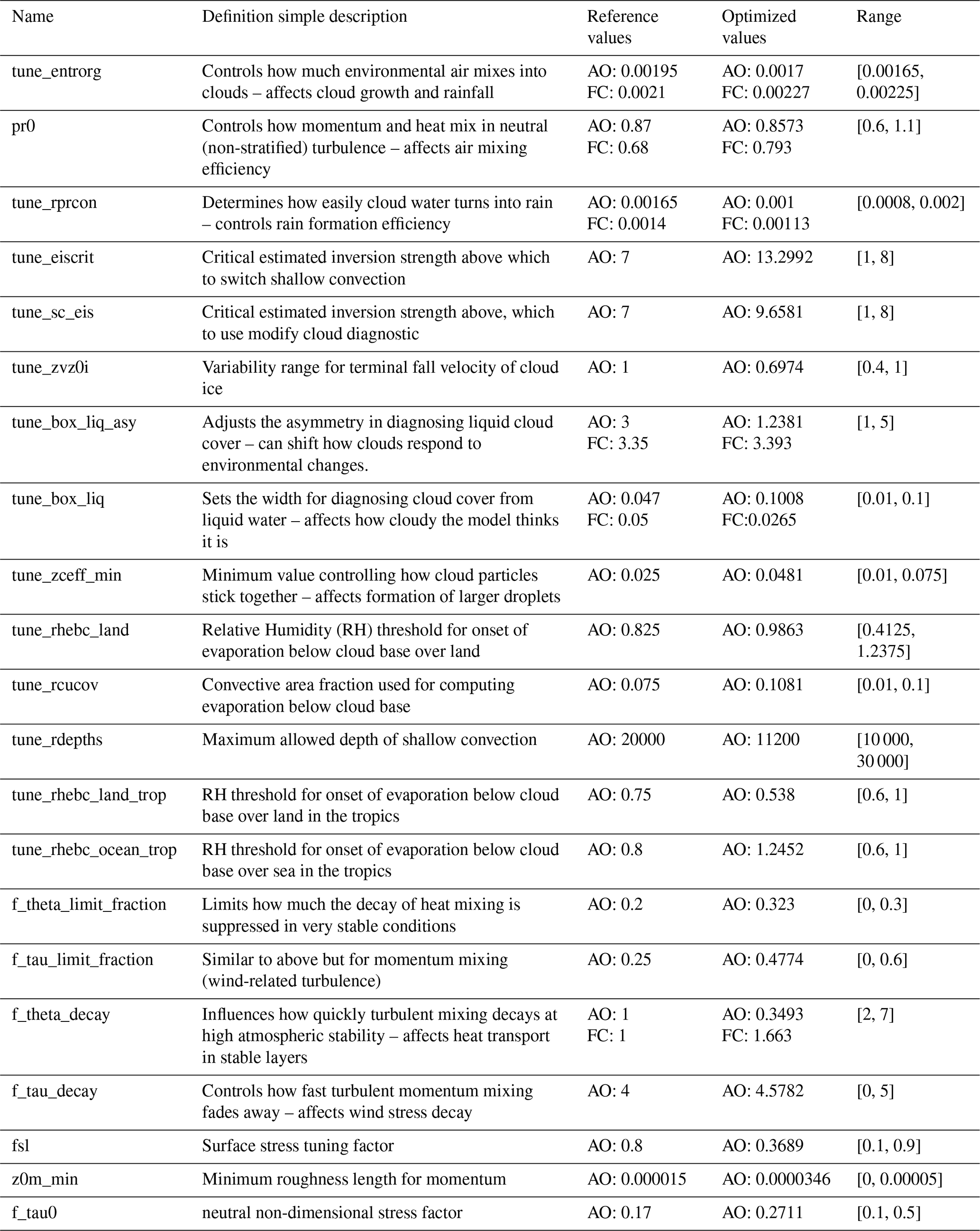
Figure 1 shows four examples of the ENSO metrics in rows for each of the three categories in columns. The climatology metrics show common model errors, such as the double ITCZ bias (Fig. 1A1), which appears as excessive precipitation in the southern hemisphere tropics, both in atmosphere-only and fully coupled reference run. An important caveat is that a pronounced double-ITCZ persists in the atmosphere-only configuration, even with observed SSTs prescribed. This implies that a significant fraction of the bias is generated within the atmospheric and land-surface components themselves. Equatorial precipitation errors (Fig. 1A2) illustrate further discrepancies in tropical rainfall patterns. Fully coupled simulations show less precipitation compared with observation, and the atmosphere-only experiments overestimate the precipitation. The cold tongue bias, a persistent issue where fully coupled models underestimate equatorial SST, is apparent in Fig. 1A3. The minimum of equatorial SST is also shifted west in the fully coupled model results. Zonal wind stress biases (Fig. 1A4) reveal substantial discrepancies in both the magnitude and position of the trade-wind maximum, which appears displaced too far west in the fully coupled simulation and too far east in the atmosphere-only experiment.

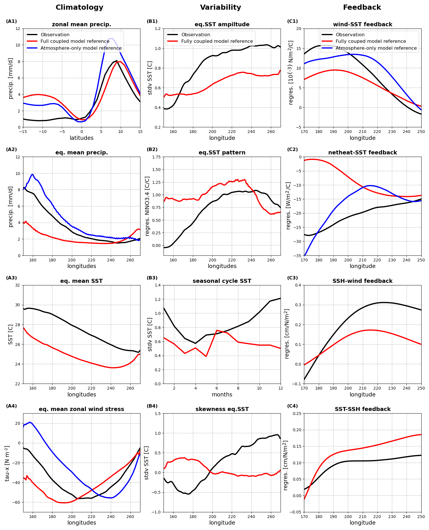
Figure 1 Comparison of some ENSO Metrics for Observations (black), ICON atmosphere-only model (blue), and ICON fully coupled (red) reference simulations for climatology (A1–A4), variability (B1–B4) and feedback (C1–C4). The metrics definition can be found in Planton et al. (2021).

In terms of ENSO variability, the ICON XPP fully coupled reference run underestimates key features of ENSO behavior. The ENSO amplitude is too weak (Fig. 1B1), the spatial pattern of SSTA is too zonally confined and shifted westward (Fig. 1B2), and the seasonality of ENSO variance is misrepresented, particularly in showing unrealistic peak during May to September and failing to capture the sharp September–February peak (Fig. 1B3). The ENSO skewness (Fig. 1B4), reflecting nonlinear asymmetry between El Niño and La Niña, is longitudinally out-of-phase and strongly underestimated. Most ENSO feedbacks (Fig. 1C1–C3) are persistently underestimated.

Critically, ENSO feedbacks (Fig. 1C1–C4) are persistently underestimated. The Bjerknes feedback (zonal wind stress response to SSTA) and thermal damping feedback (net surface heat flux response to SSTA) are weaker than observed (Fig. 1C1 and C2). Additionally, ocean coupling metrics involving SSH-SST and SSH-wind stress correlations (Fig. 1C3 and C4) show that coupled ICON XPP model fails to reproduce realistic the 1B1) and skewness (Fig. 1B4) and are tied to overly strong mean upwelling and cold SSTs (cold tongue bias, Fig. 1A3).

In the atmosphere-only simulations, only 8 ENSO metrics that measure atmospheric variables can be used to evaluate the model performance. Five of these are shown in Fig. 1, and the other three are the seasonal cycles of the zonal and eq. mean precipitation, and the eq. mean zonal wind stress. We can notice that the model biases in the atmosphere-only simulations are substantially different from those in the fully coupled simulations (Fig. 1), suggesting that the coupling between ocean and atmosphere lead to substantial changes in model biases.

3.2 Parameter sensitivities

The sensitivity of the ENSO-metrics to each tuning parameter of the ICON model is estimated by a set of perturbed parameter runs (detail see Sect. 2.3). For example, Fig. 2 illustrates the sensitivity in atmosphere-only experiments associated with the cloud conversion threshold for cloud water to rain (tune_rprcon) and the cloud asymmetry factor parameters (tune_box_liq_asy). Here the atmosphere-only control run is our reference for which we change a single parameter relative the value of the control run.

Figure 2 ENSO metric of Pacific zonal mean precipitation (A1, A3, B1, B3) and zonal wind-SST regression (A2, A4, B2, B4) for observations (black), reference atmosphere-only run (blue) and perturbed cloud conversion threshold (tune_rprcon) parameters for atmosphere-only runs (red). (A3, A4) Correspond sensitivity estimate for each perturbation runs (thin red lines); the ensemble means of them (thick red line) and the reference bias (blue line). (B1)–(B4) are for cloud asymmetry factor parameter (tune_box_liq_asy).

We can estimate the sensitivities of the ICON model (λ) to each parameter (p) and for each ENSO metric (m):

$$\begin{array}{}\text{(1)}& {\mathit{\lambda }}_{\mathrm{p}}^{\mathrm{m}}\left(\mathit{\phi }\right)={\displaystyle \frac{\mathrm{d}\mathit{\xi }}{\mathrm{d}p}}\left(\mathit{\phi }\right)\approx {\displaystyle \frac{\mathrm{\Delta }\mathit{\xi }}{\mathrm{\Delta }p}}\left(\mathit{\phi }\right).\end{array}$$

Here ξ is the physical variable measured by the ENSO metric m (e.g., precipitation as in Fig. 2A1 and B1, and wind-SST relationship in Fig. 2A2 and B2) and φ is the physical dimension the metric is depending on (e.g., latitudes). Δξ is the change in ξ relative to the control run, which means $\frac{\mathrm{\Delta }\mathit{\xi }}{\mathrm{\Delta }p}\left(\mathit{\phi }\right)=\frac{{\mathit{\xi }}_{{\mathrm{p}}_j}^{\mathrm{m}}\left(\mathit{\phi }\right)-{\mathit{\xi }}_{\mathrm{ctrl}}^{\mathrm{m}}\left(\mathit{\phi }\right)}{p_j-p_{\mathrm{ctrl}}}$, p_j is the value of parameter p value in one of the ensemble experiments, p_ctrl is the value of parameter p in the control experiment.

The Root Mean Square (RMS) error of the control run to the observation is given by rms_ctrl:

$$\begin{array}{}\text{(2)}& {\mathrm{rms}}_{\mathrm{ctrl}}=\sqrt{{\displaystyle \frac{\mathrm{1}}{N}}\sum _{i=\mathrm{1}}^N{\left({\mathit{\xi }}_{\mathrm{ctrl}}\left({\mathit{\phi }}_i\right)-{\mathit{\xi }}_{\mathrm{obs}}\left({\mathit{\phi }}_i\right)\right)}^{\mathrm{2}}}\end{array}$$

where N is the number of grid points or time steps along the dimension φ_i (e.g., latitude, longitude, or month), ξ_ctrl is the metric value in control simulation, and ξ_obs is the corresponding observed value. Hence, a smaller RMS error value means the model agrees better with observations.

The RMS amplitude of the mean sensitivity ${\mathit{\lambda }}_{\mathrm{p}}^{\mathrm{m}}\left(\mathit{\phi }\right)$ of ENSO metric m to parameter p is given by ${\mathrm{\Delta }}_{\mathrm{p}}^{\mathrm{m}}$:

$$\begin{array}{}\text{(3)}& {\mathrm{\Delta }}_{\mathrm{p}}^{\mathrm{m}}=\sqrt{{\displaystyle \frac{\mathrm{1}}{N}}\sum _{i=\mathrm{1}}^N{\left(\stackrel{\mathrm{‾}}{{\mathit{\lambda }}_{\mathrm{p}}^{\mathrm{m}}\left({\mathit{\phi }}_i\right)}\right)}^{\mathrm{2}}}=\sqrt{{\displaystyle \frac{\mathrm{1}}{N}}\sum _{i=\mathrm{1}}^N{\left({\displaystyle \frac{\mathrm{1}}{P}}\sum _{j=\mathrm{1}}^P{\mathit{\lambda }}_{{\mathrm{p}}_j}^m\left({\mathit{\phi }}_i\right)\right)}^{\mathrm{2}}}.\end{array}$$

where ${\mathit{\lambda }}_{\mathrm{p}}^{\mathrm{m}}\left({\mathit{\phi }}_i\right)=\frac{\mathrm{\Delta }{\mathit{\xi }}_{\mathrm{p}}^{\mathrm{m}}\left({\mathit{\phi }}_i\right)}{\mathrm{\Delta }p}$ is the sensitivity of metric m to parameter p at grid point φ_i, the overbar $\stackrel{\mathrm{‾}}{(\cdot )}$ denotes the ensemble mean over multiple perturbation runs, and P means the number of ensemble runs for each parameter p. Hence, in simpler terms, ${\mathrm{\Delta }}_{\mathrm{p}}^{\mathrm{m}}$ quantifies how strongly the model metric changes on average, when parameter p is perturbed. Larger ${\mathrm{\Delta }}_{\mathrm{p}}^{\mathrm{m}}$ means stronger parameter influence on that ENSO metric.

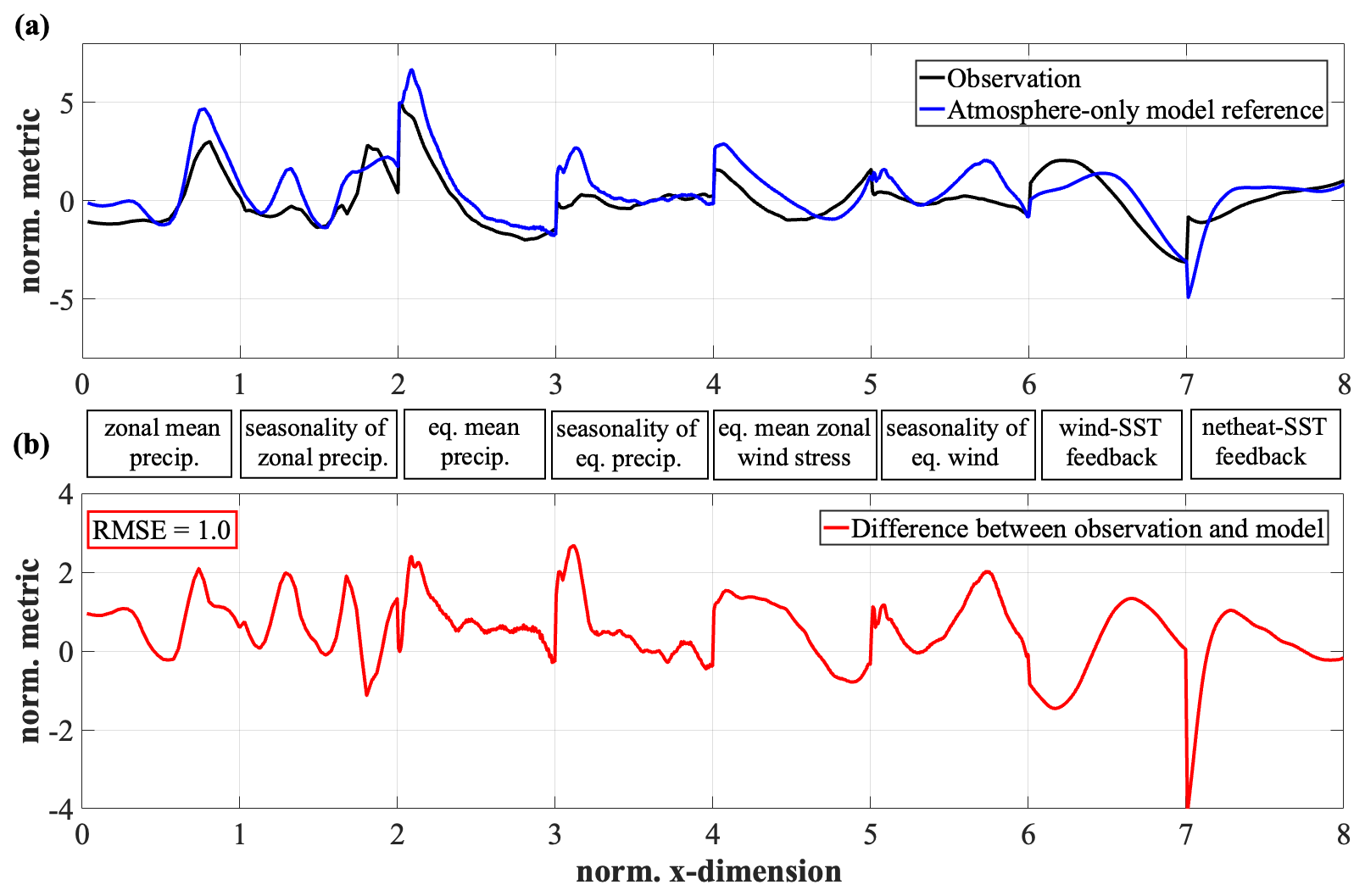
Figure 3 Normalized and combined ENSO metric for the atmosphere-only simulations. (a) shows the observed (black) and atmosphere-only simulation (blue) values of the combined ENSO metric. The x axis is a combined dimension of the 8 ENSO metrics used for atmosphere-only simulations with the labels marking which part of the x axis corresponds to which ENSO metric. (b) shows the difference between the atmosphere-only model run and the observations (red) with the RMSE value shown in the upper left corner. For 0–1, zonal mean precipitation; 1–2, seasonality of zonal precipitation; 2–3, equatorial mean precipitation; 3–4, seasonality of equatorial precipitation; 4–5, equatorial mean zonal wind stress; 5–6, seasonality of equatorial wind; 6–7, wind-SST feedback; 7–8, net heat-SST feedback.

The uncertainty of the sensitivities among individual perturbed ensemble members is given by std(${\mathrm{\Delta }}_{\mathrm{p}}^{\mathrm{m}}$):

$$\begin{array}{}\text{(4)}& \mathrm{std}\left({\mathrm{\Delta }}_{\mathrm{p}}^{\mathrm{m}}\right)=\sqrt{{\displaystyle \frac{\mathrm{1}}{P-\mathrm{1}}}\sum _{j=\mathrm{1}}^P{\left({\mathrm{\Delta }}_{{\mathrm{p}}_j}^{\mathrm{m}}-\stackrel{\mathrm{‾}}{{\mathrm{\Delta }}_{\mathrm{p}}^{\mathrm{m}}}\right)}^{\mathrm{2}}},\end{array}$$

where ${\mathrm{\Delta }}_{{\mathrm{p}}_j}^{\mathrm{m}}=\sqrt{\frac{\mathrm{1}}{N}\sum _{i=\mathrm{1}}^N(\stackrel{\mathrm{‾}}{{\mathit{\lambda }}_{{\mathrm{p}}_j}^{\mathrm{m}}\left({\mathit{\phi }}_i\right)}{)}^{\mathrm{2}}}$ is the sensitivity for one ensemble member j and $\stackrel{\mathrm{‾}}{{\mathrm{\Delta }}_{\mathrm{p}}^{\mathrm{m}}}=\frac{\mathrm{1}}{P}\sum _{j=\mathrm{1}}^P{\mathrm{\Delta }}_{{\mathrm{p}}_j}^{\mathrm{m}}$ is the ensemble mean of sensitivity over multiple perturbation runs. Hence, std(${\mathrm{\Delta }}_{\mathrm{p}}^{\mathrm{m}}$) represents how consistent the sensitivity is across different perturbations. If std(${\mathrm{\Delta }}_{\mathrm{p}}^{\mathrm{m}}$) is small, the response of metric m to parameter p is consistent and reliable across different perturbations. If it is large, the model's response changes unpredictably between perturbations, which may result from the model nonlinearities or interactions with other parameters. Finally, the signal to noise ratio is given by $r_{\mathrm{p}}^{\mathrm{m}}=\frac{{\mathrm{\Delta }}_{\mathrm{p}}^{\mathrm{m}}}{\mathrm{std}\left({\mathrm{\Delta }}_{\mathrm{p}}^{\mathrm{m}}\right)}$. It compares the mean signal strength (the systematic sensitivity) to the ensemble spread (randomness or uncertainty). If $r_{\mathrm{p}}^{\mathrm{m}}>\mathrm{1}$), it means parameter p has strong, robust, and consistent sensitivity on ENSO metric m. If $r_{\mathrm{p}}^{\mathrm{m}}<\mathrm{1}$, it means the sensitivity is weak or inconsistent, likely obscured by noise.

Figure 2A3 shows the estimated values of ${\mathit{\lambda }}_{\mathrm{p}}^{\mathrm{m}}\left(\mathit{\phi }\right)$ on the meridional precipitation structure for the cloud conversion threshold parameter perturbation runs and the ensemble mean. Note, ${\mathit{\lambda }}_{\mathrm{p}}^{\mathrm{m}}=\frac{{\mathit{\xi }}_{{\mathrm{p}}_j}^{\mathrm{m}}\left(\mathit{\phi }\right)-{\mathit{\xi }}_{\mathrm{ctrl}}^{\mathrm{m}}\left(\mathit{\phi }\right)}{p_j-p_{\mathrm{ctrl}}}$ is a sensitivity in $\mathit{\xi }/p$ relative to the control atmosphere-only run. It does not consider the observed values and is therefore not measuring a bias. It only estimates if $\mathit{\xi }/p$ would increase or decrease relative to the control run. We can further see that not all perturbed parameter runs result into the same ${\mathit{\lambda }}_{\mathrm{p}}^{\mathrm{m}}$, leading to some spread. This spread gives us some indication of how uncertain these sensitivity estimates are which we can use later for the optimization scheme. In the example shown in Fig. 2A1 we can note that the tuning parameter has a significant influence on the tropical precipitation simulation, in particular at latitudes around 7° N, and a $r_{\mathrm{p}}^{\mathrm{m}}>\mathrm{1}$, which suggests a significant signal to noise ratio. The sensitivity of different ENSO metrics varies across parameters. For instance, the cloud conversion threshold for cloud water to rain shows a stronger impact on meridional precipitation structure (Fig. 2A3, $r_{\mathrm{p}}^{\mathrm{m}}=\mathrm{2.06}$) than on the wind–SST correlation (Fig. 2A4, $r_{\mathrm{p}}^{\mathrm{m}}=\mathrm{1.44}$). In contrast, the cloud asymmetry factor exhibits weaker sensitivities $r_{\mathrm{p}}^{\mathrm{m}}$ for both metrics (Fig. 2B3 and B4) compared to the cloud conversion threshold (Fig. 2A3 and A4).

Since the ENSO metrics differ in both magnitude and physical dimension, all metrics are combined into a single composite normalized curve to allow the misfit to be minimized through a single scalar quantity. For example, for each metric m in the atmosphere-only experiments, we first compute the model–observation difference Δξ_m(φ) along its natural one-dimensional axis φ (e.g., latitude for zonal-mean quantities in Fig. 1A1, longitude for equatorial averages in Fig. 1A2, A4, C1 and C2), then (i) normalize the amplitude by the RMSE of the atmosphere-only control, ${\widehat{\mathrm{\Delta }\mathit{\xi }}}_{\mathrm{m}}\left(\mathit{\phi }\right)=\mathrm{\Delta }{\mathit{\xi }}_{\mathrm{m}}\left(\mathit{\phi }\right)/{\mathrm{rms}}_{\mathrm{ctrl}}$; and (ii) normalize the axis φ to unit length, $\widehat{\mathit{\phi }}\in [\mathrm{0},\mathrm{1}]$. The eight normalized metric segments are concatenated sequentially to construct a single composite curve χ(ψ) defined over $\mathit{\psi }\in [\mathrm{0},\mathrm{8}]$ (Fig. 3). By design, the composite RMSE of the control simulation equals 1.0 (Fig. 3b). The optimization scheme therefore aims to minimize the amplitude (RMSE) of χ(ψ), representing the aggregated ENSO-model misfit across all metrics.

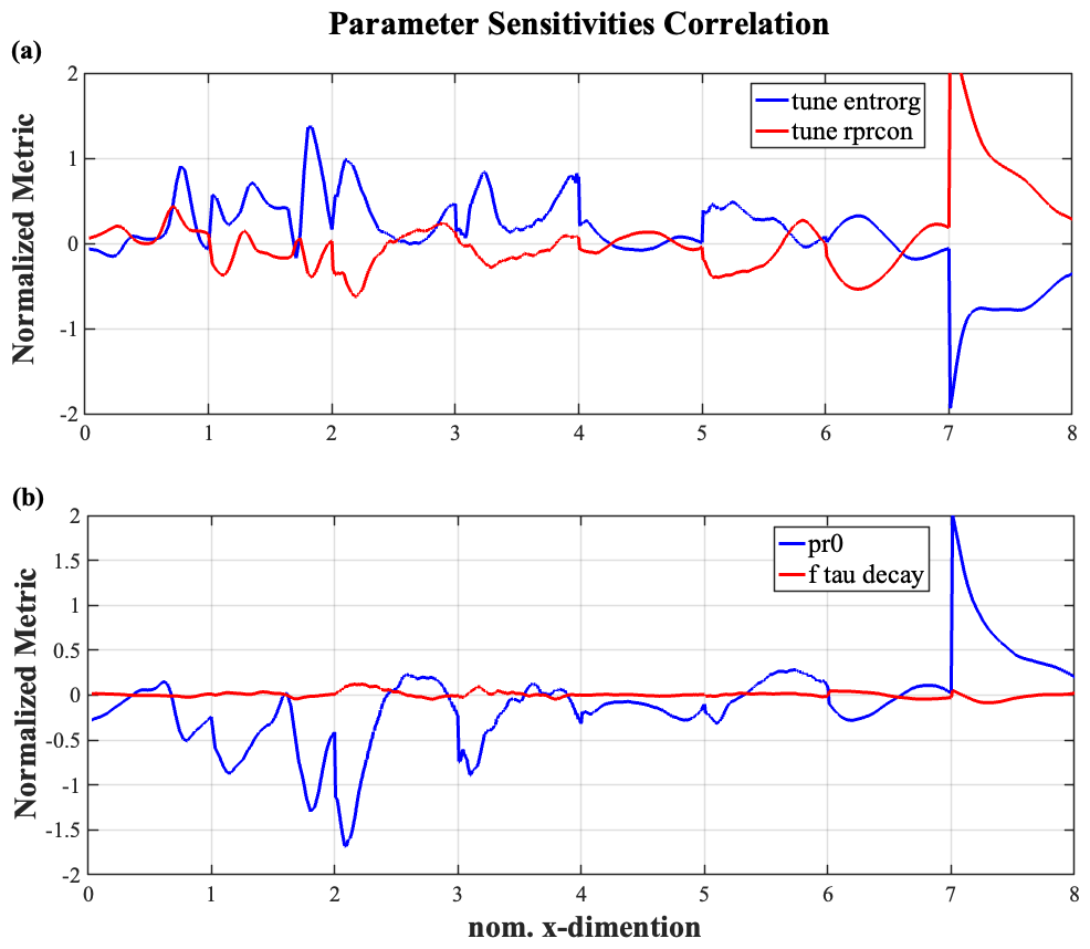
Figure 4 Normalized sensitivity of the combined ENSO metrics in atmosphere-only runs for four different tuning parameters, (a) tune_entrorg and tune_rprcon; (b) pr0 and f_tau_decay. The correlation between the pair of sensitivities is −0.83 in (a) and −0.55 in (b). The normalized x-dimension has the same definition as in Fig. 3.

The sensitivity ${\mathit{\lambda }}_{\mathrm{p}}^{\mathrm{m}}$ will also be normalized by $\widehat{{\mathit{\lambda }}_{\mathrm{p}}^{\mathrm{m}}}=\frac{\mathrm{\Delta }\widehat{\mathit{\xi }}}{\mathrm{\Delta }p}\left(\widehat{\mathit{\phi }}\right)$. Because $\widehat{{\mathit{\lambda }}_{\mathrm{p}}^{\mathrm{m}}}$ depends on the specific range of each model parameter p, direct comparison across parameters is not meaningful without further normalization. To ensure comparability, the sensitivities are standardized according to

$$\begin{array}{}\text{(5)}& n\widehat{{\mathit{\lambda }}_{\mathrm{p}}^{\mathrm{m}}}={\displaystyle \frac{\widehat{{\mathit{\lambda }}_{\mathrm{p}}^{\mathrm{m}}}}{{\mathit{\sigma }}_{\mathrm{p}}}}\end{array}$$

here σ_p is the standard deviation of the perturbed parameters p, which is approximated as ¼ of the parameter range in Table 1.

Figure 4a and b shows examples of the normalized sensitivities $n\widehat{{\mathit{\lambda }}_{\mathrm{p}}^{\mathrm{m}}}$ for four representative tuning parameters across the eight combined ENSO metrics in the atmosphere-only simulations. Each sensitivity is scaled by the RMS error of the corresponding metric in the control run (e.g., rms_ctrl in Fig. 3A2 and A4), enabling a direct comparison across different ENSO metrics. The sensitivities reveal that different parameters influence ENSO-related processes with distinct amplitudes and spatial structures, yet many exhibit broadly similar patterns of response. This similarity is quantified by the strong cross-correlations between parameter sensitivities (−0.83 in Fig. 4a and −0.55 in Fig. 4b), indicating that several parameters act in comparable directions within the ENSO-related error space. In practical terms, such strong correlations imply that the effective degrees of freedom available for independent tuning are reduced: modifying one parameter may partially replicate the effect of another, limiting the uniqueness of the optimization solution.

Conversely, parameters that display weak or spatially incoherent sensitivities (e.g., f_tau_decay in Fig. 4b) contribute less to ENSO variability and exert limited leverage on the overall ENSO metrics. This suggests that not all tunable parameters are equally influential, and that focusing on the few parameters with large, structured sensitivities provides a more efficient path for improving ENSO performance. Together, these results demonstrate that the ENSO-related model behavior in the atmosphere-only configuration is controlled by a small subset of interdependent parameters rather than by the full ensemble of 21 tested parameters.

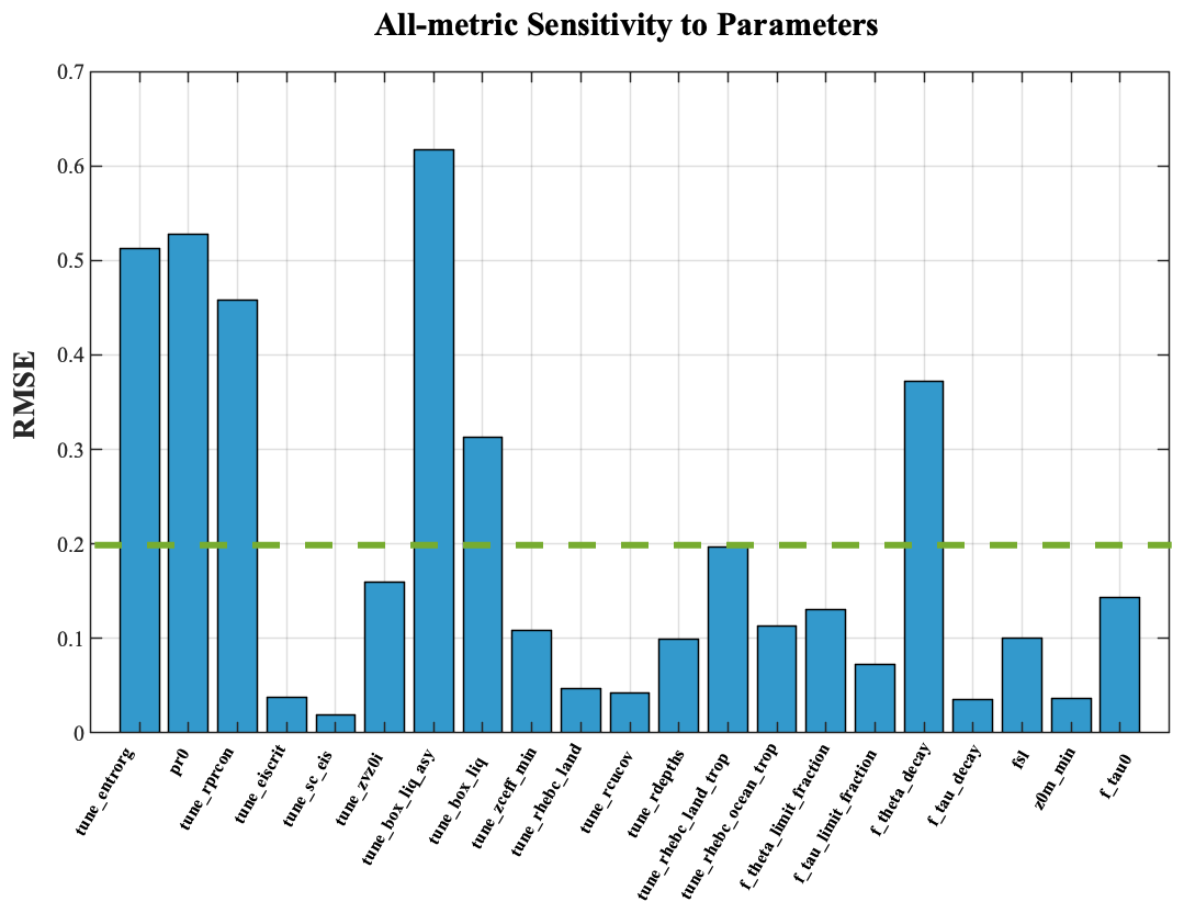
Figure 5 Mean RMS values of the sensitivity of the combined ENSO metrics in atmosphere-only runs for all 21 parameters. The x axis shows parameter names, and the y axis shows the RMSE-based sensitivity value. A mean RMS sensitivity of 1.0 refers to a sensitivity as strong in amplitude as the atmosphere-only control run biases. Parameters exhibiting RMSE values above the threshold of 0.2 (horizontal green dashed line) are considered to have significant impacts on ENSO simulation during the atmosphere-only model tuning phase.

Figure 5 shows the RMS value of the scaled $n\widehat{{\mathit{\lambda }}_{\mathrm{p}}^{\mathrm{m}}}$, averaged over all eight ENSO metrics for the atmosphere-only simulations. A mean RMS value of 1.0 corresponds to a sensitivity magnitude comparable to the ENSO-related bias of the control run, implying that perturbing a parameter by one standard deviation (σ_p) would alter the ENSO metric by an amount similar in strength to the model bias, though not necessarily with the same spatial pattern (cf. Fig. 3A2 and A4). Among the 21 tested parameters, only about six exhibit pronounced impacts on the ENSO metrics, exceeding an RMS threshold of 0.2. This threshold was empirically determined as a practical cutoff corresponding to roughly 20 % of the control-run bias amplitude – large enough to isolate parameters with meaningful physical influence, yet small enough to avoid spurious noise from weak sensitivities. We emphasize that 0.2 is a pragmatic screening threshold rather than a theoretically optimal or universal cutoff. This interpretation is consistent with common tuning and sensitivity-screening practice, where relative criteria are used to identify influential parameters (e.g., Hourdin et al., 2017; Williamson et al., 2013; Murphy et al., 2004).

Given that these six parameters also display high inter-correlation in their sensitivity patterns (e.g., Fig. 4a and b), the effective number of independent parameters controlling ENSO behavior in the atmosphere-only configuration is likely much smaller than 21, and probably closer to two. This finding underscores that ENSO biases in the atmospheric component are governed by a limited subset of strongly interacting parameters, rather than by many independent degrees of freedom.

3.3 Cost function

The cost function quantifies the overall model–observation misfit while penalizing large deviations in the parameter space. It is defined as a positive-definite function, with smaller values indicating a better fit to observations. For both atmosphere-only and fully coupled experiments, the cost function consists of three components:

$$\begin{array}{}\text{(6)}& f_{\mathrm{cost}}={\mathrm{\Delta }}_{\mathrm{limit}}\left({\mathrm{\Delta }}_{\mathrm{metric}}+{\mathrm{\Delta }}_{\mathrm{para}}\right).\end{array}$$

Δ_metric quantifies how well the ENSO metrics are simulated:

$$\begin{array}{}\text{(7)}& {\mathrm{\Delta }}_{\mathrm{metric}}=\sum _{m=\mathrm{1}}^M{\mathit{\omega }}_{\mathrm{m}}{\displaystyle \frac{{\mathit{\delta }}_{\mathrm{m}}}{{\mathit{\delta }}_{{\mathrm{ctrl}}_{\mathrm{m}}}}}/\sum _{m=\mathrm{1}}^M{\mathit{\omega }}_{\mathrm{m}}.\end{array}$$

Here, ${\mathit{\delta }}_{\mathrm{m}}=\sqrt{\frac{\mathrm{1}}{N}\sum _{i=\mathrm{1}}^N\left({\mathit{\xi }}_{\mathrm{ens},\mathrm{m}}\right({\mathit{\phi }}_i)-{\mathit{\xi }}_{\mathrm{obs},\mathrm{m}}({\mathit{\phi }}_i){)}^{\mathrm{2}}}$ is the RMS error of metric m (as defined in Planton et al., 2021) in the ensemble experiments, and ${\mathit{\delta }}_{\mathrm{ctrl},\mathrm{m}}=\sqrt{\frac{\mathrm{1}}{N}\sum _{i=\mathrm{1}}^N\left({\mathit{\xi }}_{\mathrm{ctrl},\mathrm{m}}\right({\mathit{\phi }}_i)-{\mathit{\xi }}_{\mathrm{obs},\mathrm{m}}({\mathit{\phi }}_i){)}^{\mathrm{2}}}$ is the corresponding RMS error in the control run (cf. Fig. 3b), M is the number of ENSO metrics, which is 8 in the atmosphere-only and 17 in the fully coupled experiments. This normalization is necessary because the ENSO metrics differ in units and amplitude. Although using the control-run uncertainty as a normalization factor is a pragmatic choice rather than an optimal one, it provides a first-order approximation. Each metric is weighted by ω_m, which determines its relative importance (set to 1 in this study for equal weighting).

The second term, Δ_para, penalizes large deviations of the tuning parameters from their control values:

$$\begin{array}{}\text{(8)}& {\mathrm{\Delta }}_{\mathrm{para}}={\mathit{\alpha }}_{\mathrm{para}}{\displaystyle \frac{\mathrm{1}}{K}}\sum _{k=\mathrm{1}}^K{\left(\mathrm{\Delta }n{p}_k\right)}^{\mathrm{4}}\end{array}$$

with K the total number of perturbed parameters, which is 21 in the atmosphere-only and 6 in the fully coupled experiments. p_k are the parameters that are tuned in this study (e.g. tune_entrorg, pr0, tune_rprcon in Table 1). Δnp_k is the normalized parameter change relative to the control run:

$$\begin{array}{}\text{(9)}& \mathrm{\Delta }n{p}_k={\displaystyle \frac{\mathrm{\Delta }{p}_k}{{\mathit{\sigma }}_{{\mathrm{para}}_k}}}={\displaystyle \frac{p_k-p_{\mathrm{ctrl}}}{{\mathit{\sigma }}_{{\mathrm{para}}_k}}}.\end{array}$$

In Eq. (8) we use the power of 4 to allow for small changes in the parameter without increasing the cost function. α_para=0.01, is a scaling parameter to determine the relative importance of model parameter deviations from the control with respect to the importance of Δ_metric. The reference parameter set is not assumed to represent a physically optimal state, but rather a numerically stable baseline configuration for each model setup (atmosphere-only or fully coupled). In this sense, Eq. (8) acts as a regularization term that constrains optimization to a physically plausible neighborhood of the corresponding control configuration, thereby preventing unrealistic parameter excursions and overfitting of the ENSO metrics. In practice, the optimized parameter values remain within a limited range of their corresponding control values, indicating that the optimization does not rely on large departures from the baseline state.

Finally, the constraint term Δ_limit ensures that parameters remain within physically meaningful bounds (e.g., positive-definite quantities):

$$\begin{array}{}\text{(10)}& {\mathrm{\Delta }}_{\mathrm{limit}}=n_{\mathrm{limit}}+\mathrm{1}\end{array}$$

where n_limit counts the number of parameters that violate predefined physical bounds within a given parameter combination p_k. In this study, the key hard bound is positivity for selected parameters. For example, if in one candidate parameter set p_k, two parameters take negative values that violate positive-definite constraints, then Δ_limit=3, which substantially increases f_cost. In practice, the optimization workflow checks each candidate parameter combination and excludes combinations that violate these physical bounds.

Importantly, these hard physical bounds are distinct from the parameter ranges listed in Table 1. The Table 1 ranges are perturbation intervals used to estimate sensitivities in the ensemble experiments and are not applied as strict bounds during optimization. In this sense, the parameter-deviation term in Eq. (8) acts as a soft regularization constraint, whereas Eq. (10) provides a hard physical-bound constraint. Optimized values that fall outside listed Table 1 ranges therefore mainly occur near or slightly beyond the edge of the initial sampling space; these deviations are moderate and do not lead to physically unrealistic model behavior.

3.4 Approximating the ENSO metrics

Directly estimating Δ_metric requires rerunning the ICON model to compute each δ_m, which is computationally expensive. As an alternative, we approximate Δ_metric using the pre-calculated parameter sensitivities $n\widehat{{\mathit{\lambda }}_{\mathrm{p}}^{\mathrm{m}}}$, under the assumption that the bias in each metric, δ_m, can be represented as a linear combination of these sensitivities:

$$\begin{array}{}\text{(11)}& {\mathit{\delta }}_{\mathrm{m}}\approx {\mathit{\delta }}_{\mathrm{m}}^{\mathrm{approx}}=\sum _{k=\mathrm{1}}^K{\displaystyle \frac{r_{{\mathrm{p}}_k}^{\mathrm{m}}}{r_{{\mathrm{p}}_k}^{\mathrm{m}}+\mathrm{0.3}}}\mathrm{\Delta }n{p}_k\cdot n\widehat{{\mathit{\lambda }}_{\mathrm{p}}^{\mathrm{m}}}.\end{array}$$

Each sensitivity is weighted by its confidence ratio $r_{{\mathrm{p}}_k}^{\mathrm{m}}$, as shown by $r_{\mathrm{p}}^{\mathrm{m}}$ in Fig. 3b, to account for uncertainty in the sensitivity estimates. Parameters with low signal-to-noise ratios ($r_{{\mathrm{p}}_k}^{\mathrm{m}}$) contribute less to the cost function, ensuring that uncertain or noisy sensitivities exert limited influence on the optimization.

Equation (11) is a first-order approximation of how the model–observation misfit changes under parameter perturbations, rather than an exact identity of the nonlinear ENSO metric itself. The ENSO metrics are computed from model–observation differences (e.g., RMSE), which are nonlinear, while the right-hand side of Eq. (11) represents a linearized estimate of model-response changes based on pre-computed sensitivities.

Conceptually, the procedure is to (i) approximate parameter-induced changes in model variables around a reference state using linear sensitivities, (ii) evaluate how this linearized model change modifies the model–observation misfit with observations kept fixed, and (iii) use the result as a surrogate objective for optimization. Therefore, Eq (11) should be interpreted as a linearized misfit-change estimate.

This approximation neglects higher-order nonlinear effects in both model response and metric definition, and is expected to be most accurate for a local neighborhood of the control state with moderate parameter perturbations. In this study, this practical range is represented by the parameter-perturbation intervals used to estimate sensitivities (Table 1), with sensitivities evaluated around the control simulation as a numerically stable baseline.

Because Eq. (11) omits explicit cross-parameter interaction terms, it can introduce approximation error and may shift the estimated optimum relative to a fully nonlinear search. We therefore interpret Eq. (11) as a computationally efficient first-order surrogate for screening and optimization, and assess the final parameter choices with full model integrations. Observations do not depend on model parameters and are used only to define the optimization target (misfit/cost function).

3.5 Optimization scheme

The optimization process seeks to minimize f_cost using the Nelder–Mead simplex method (Nelder and Mead, 1965; Luersen and Le Riche, 2004), a derivative-free algorithm that efficiently searches parameter space through iterative geometric transformations – reflection, expansion, contraction, and shrinkage. In this implementation, f_cost is evaluated using the linear approximation ${\mathit{\delta }}_{\mathrm{m}}^{\mathrm{approx}}$, which avoids the need to rerun the ICON model for each parameter combination and thereby reduces computational expense by several orders of magnitude. The optimization is initialized from a single starting point given by the control parameter set, which provides a physically calibrated and numerically stable baseline. The algorithm then progressively adjusts the parameter ensemble until a local minimum of f_cost is reached, typically requiring around 1000 candidate parameter evaluations. Because Nelder–Mead is a local method, different initial points could in principle converge to different local minima; however, the present goal is robust local improvement relative to the control state rather than global-optimum identification. Exploring multi-start or global optimization strategies is left for future work.

4 Results for atmosphere-only experiments

4.1 Performance of the optimized atmosphere-only configuration

The initial tuning phase in this study involves perturbing 21 atmospheric parameters individually to systematically evaluate their sensitivities using atmosphere-only simulations. Each parameter's sensitivity is estimated by analyzing its impact on various ENSO metrics, following the method outlined in Sect. 3.2. The optimization process (Sect. 3) finds a set of optimal values for all 21 parameters (Table 1) that minimize the cost function Eq. (6). Figure 6 shows the normalized and combined ENSO metrics performance for the atmosphere-only run with the optimized parameters and for the atmosphere-only reference run.

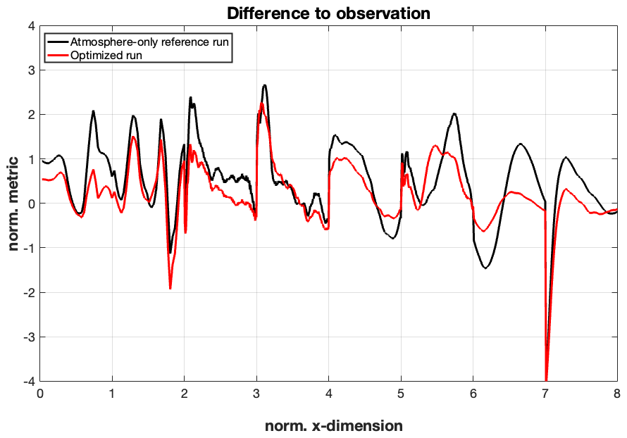
Figure 6 Normalized and combined ENSO metrics in atmosphere-only simulations for a simulation with the atmosphere-only reference parameters (black) and for a run with 21 optimized parameters (red). A zero value suggests a match to the observed reference. The normalized x-dimension has the same definition as in Fig. 3.

The ENSO metrics of the optimized atmosphere-only run are nearly always closer to zero than the control run, suggesting improvements in nearly all metrics for nearly all regions. The overall RMSE error reduced substantially from 1.0 to 0.73. We can further notice the two ENSO metric curves are similar (corr. = 0.85; Fig. 6), suggesting that the structures of the biases are the same in the control and the optimized run. This means that persistent biases such as the double ITCZ or the too weak wind-SST feedback are still present in the optimized run, but have significantly reduced magnitudes.

4.2 Improvement in global climate beyond the cost function

The optimization scheme by construction reduces the value of the f_cost (Eq. 6), which can only be achieved by reducing the value of Δ_metric (Eq. 7). Thus, it is by construction that the optimized atmosphere-only run will have a smaller RMSE than the control atmosphere-only run in ENSO metric values shown in Fig. 6. While the improvements in the ENSO metric are substantial, it is still important to verify that the model simulations improve beyond the characteristics of the climate directly quantified by Δ_metric. This can be done by evaluating the climate simulations beyond the Pacific domain, as none of the metrics included in Δ_metric consider climate variables beyond the Pacific domain.

Figure 7 compares the annual-mean biases in precipitation and surface wind stress between the reference and optimized atmosphere-only runs. The analysis also summarizes area-weighted RMS errors across three regions: the tropics excluding the Pacific (15° S–15° N, outside 150–270° E), the Northern Hemisphere extratropic (30–60° N), and the Southern Hemisphere extratropic (30–60° S). Although the optimization was explicitly designed to reduce ENSO-related biases within the tropical Pacific, the results show clear global improvements beyond the target tropical region. Across all three regions and for all variables – precipitation, zonal wind stress, and meridional wind stress – the RMSE decreases by approximately 5 %–27 %. The largest fractional improvements occur in the tropical Atlantic–Indian sector for precipitation, along Northern Hemisphere storm-track latitudes for zonal wind stress, and over the Southern Ocean for meridional wind stress. These results demonstrate that the ENSO-focused tuning yields emergent global benefits, improving large-scale precipitation and momentum flux patterns well beyond the Pacific basin metrics directly included in the cost function.

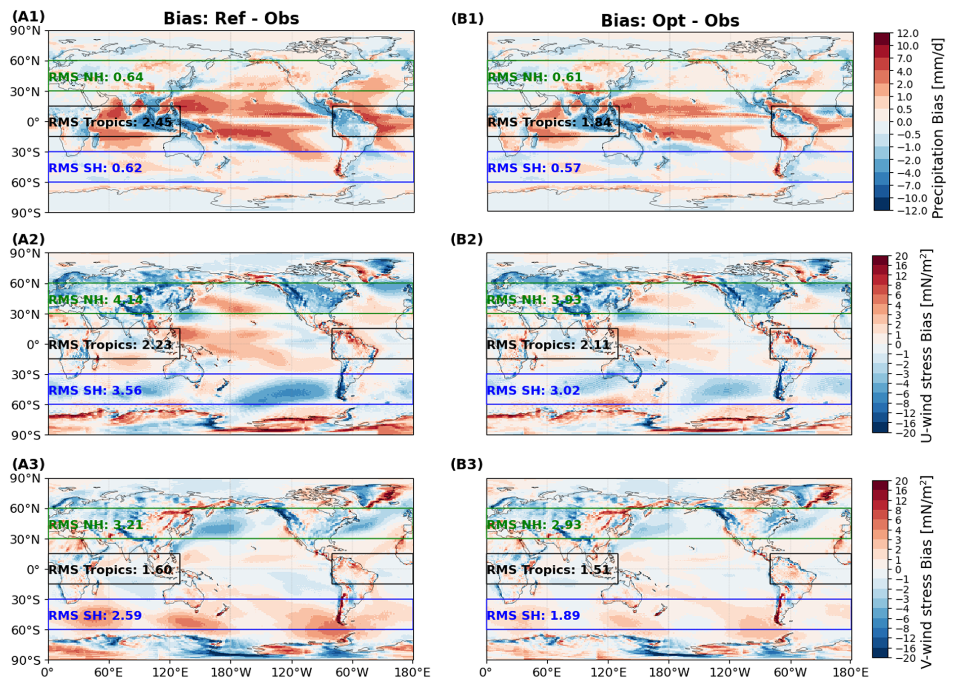
Figure 7 Global maps of annual-mean biases in precipitation (A1, B1), zonal (A2, B2) and meridional (A3, B3) wind stress for the ICON XPP atmosphere-only reference run (“Bias: Ref – Obs”, A1–A3) and optimized atmosphere-only run (“Bias: Opt – Obs”, B1–B3), relative to observational datasets. Panel annotations summarize area-weighted RMSE in three extratropic regions: (black) tropics excluding the Pacific (15° S–15° N, outside 150–270° E), (green) Northern Hemisphere extratropic (30–60° N), and (blue) Southern Hemisphere extratropic (30–60° S). RMS NH, RMS Tropics, and RMS SH represent the root mean square values of bias in Northern Hemisphere extratropic, tropics excluding the Pacific, and Southern Hemisphere extratropic, respectively. Decreases in the regional RMS metrics denote improvement.

5 Results for fully coupled experiments

5.1 Parameter sensitivity for ENSO metrics in fully coupled experiments

Despite substantial improvements achieved in atmospheric processes in atmosphere-only tuning experiments, the ENSO variability and key ENSO feedback mechanisms are naturally not represented, indicating the necessity of coupled ocean-atmosphere tuning for comprehensive ENSO simulation improvement. To address this, a second-stage tuning is conducted using fully coupled experiments. Based on the atmosphere-only sensitivity results (Fig. 5), six atmospheric parameters with the strongest impacts on ENSO metrics are selected for fully coupled tuning. Each of these parameters is perturbed individually across a range of values informed by prior sensitivity analysis listed in Table 1.

We note that this atmosphere-only pre-selection is a first-order screening strategy, not a definitive ranking of parameter importance in the fully coupled system. Because ocean–atmosphere feedbacks can alter both the magnitude and sign of sensitivities, some parameters that are weak in atmosphere-only experiments may still be influential in the fully coupled configuration. The practical motivation for atmosphere-only-based screening is computational: a full fully coupled sensitivity exploration over all candidate parameters is currently prohibitively expensive. The potential consequence is that the reduced fully coupled search space may miss some parameters that are important in the fully coupled system, even though it efficiently targets parameters with strong direct atmospheric influence on ENSO-related processes.

To further examine the necessity of direct coupled-model tuning, Fig. 8 shows the parameter sensitivity analysis to fully coupled simulations, focusing on the cloud conversion threshold (tune_rprcon) cloud asymmetry factor (tune_box_liq_asy) parameters. This analysis mirrors the atmosphere-only-based results shown in Fig. 2, enabling direct comparison of parameter impacts across configurations. In contrast to the atmosphere-only case, where perturbations to the cloud asymmetry factor showed relatively consistent impacts on tropical precipitation and feedback strength, the fully coupled simulations exhibit more muted and spatially variable responses. For example, for the cloud conversion threshold (row A in Fig. 8), the meridional precipitation structure in the eastern Pacific shows muted and latitude-shifted responses: ensemble spread is modest and the signal concentrates in the southern tropics (Fig. 8A1), whereas the atmosphere-only case showed a stronger response with a northern-hemisphere maximum (Fig. 2A1). The zonal wind-stress–SST coupling exhibits only moderate ensemble divergence in the fully coupled model (Fig. 8A2), with a weaker and less coherent mean sensitivity than in the atmosphere-only counterpart (Fig. 2A2). Once the ocean is interactive, thermocline and background-wind adjustments partly compensate the atmospheric perturbation, reducing – and sometimes relocating – the effective sensitivity. For the cloud asymmetry factor parameter (row B in Fig. 8), fully coupled responses are smaller and more spatially variable than in the atmosphere-only case. The precipitation metric (Fig. 8B1) shows weaker, patchy sensitivities, while the wind-stress–SST coupling (Fig. 8B2) has a low signal-to-noise ratio, again contrasting with the clearer signal in Fig. 2B2.

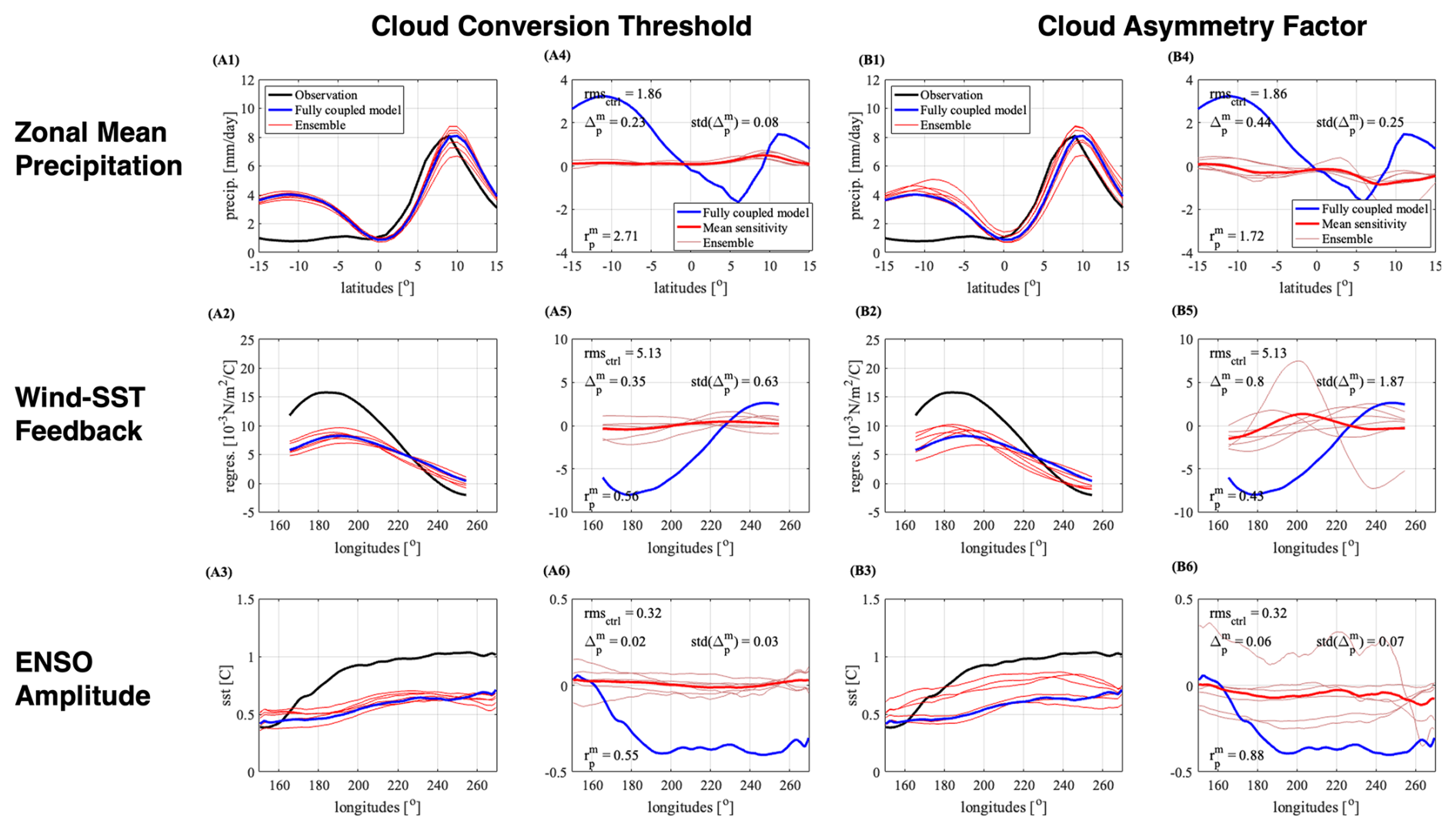
Figure 8 Sensitivity of ENSO-relevant metrics to perturbations in the cloud conversion threshold (tune_rprcon) (A1–A6) and cloud asymmetry factor parameter (tune_box_liq_asy) (B1–B6) from fully coupled simulations. Panels (A1)–(A3) and (B1)–(B3) show metric values from observations (black), ICON XPP fully coupled reference run (blue), and perturbed-parameter ensemble simulations (red), consistent with the atmosphere-only sensitivity format in Fig. 3. Corresponding sensitivity estimates are shown in panels (A4)–(A6) and (B4)–(B6), including ensemble mean sensitivity (thick red), spread (thin red), and reference bias (blue). The third row (A3, A6, B3, B6) shows ENSO amplitude, defined as the standard deviation of sea-surface temperature anomalies (SSTA) in the central equatorial Pacific, which is not included in the atmosphere-only results.

The results suggest that the cloud asymmetry factor and cloud conversion threshold interact differently with coupled ocean-atmosphere dynamics compared with atmosphere-only experiments, potentially due to compensating oceanic adjustments or altered mean state climatology. This divergence underlines the importance of conducting sensitivity analysis directly in the coupled configuration rather than relying solely on atmosphere-only-informed expectations. Actually, when the atmosphere-only optimized parameters are directly applied in coupled fully coupled simulations, they resulted in unrealistic warming of global mean surface temperature, approximately 7.3 °C higher than observations (results not shown). Therefore, direct sensitivity analyses and parameter tuning within the coupled model context are not only beneficial, but essential for realistic and stable ENSO simulation.

Figure 8 also introduces ENSO amplitude sensitivity, which is not available in atmosphere-only configuration. For the cloud asymmetry factor, the fully coupled model shows a consistent increase in ENSO variability across ensemble members (Fig. 8B3), with a positive and coherent ensemble-mean sensitivity (Fig. 8B6). This indicates that strengthening cloud asymmetry tends to amplify central-Pacific SSTA variance, i.e., it acts to increase ENSO amplitude. In contrast, the cloud conversion threshold exhibits a smaller and noisier response (Fig. 8A3 and A6): the ensemble spread is larger and the mean sensitivity is weakly positive at best, implying a limited leverage of this parameter on ENSO amplitude once the ocean is interactive.

5.2 Performance of the optimized coupled configuration

In the fully coupled optimization, we adopt the same linear sensitivity-based tuning framework used for the atmosphere-only experiments but recalculate the parameter sensitivities within the fully coupled ICON XPP model. The cost function remains structurally consistent with the atmosphere-only case, comprising a weighted sum of normalized RMSEs across selected ENSO metrics. A key difference in this stage is the broader availability of ENSO-relevant diagnostics. In contrast to the atmosphere-only case – where oceanic processes cannot be resolved and certain feedbacks cannot be computed – the fully coupled model allows us to include a complete set of ENSO metrics, as defined in the CLIVAR ENSO Metrics Package (Planton et al., 2021). Each metric is normalized by the standard deviation across the perturbed ensemble and equally weighted in the total cost. This approach enables direct comparison with atmosphere-only results while appropriately accounting for coupled dynamics.

Figure 9 illustrates the impacts of coupled-model parameter tuning on ICON XPP's ENSO-related metrics. Observations, fully coupled reference run, and optimized coupled-model experiment are compared, providing insight into how tuning selected atmospheric parameters affects ENSO simulation fidelity in the coupled framework. The optimized parameters' values $V_{\mathrm{p}}^{\mathrm{opt}}$ can be found in Table 1. A notable and concerning feature of the tuning results is that nearly all 6 parameters selected for optimization exhibit opposite directional adjustments between atmosphere-only and fully coupled simulations. Specifically, parameter values that required increases in atmosphere-only tuning (e.g., entrainment rate or cloud asymmetry factor) are found to require reductions in the fully coupled tuning, and vice versa. This reversal suggests that the nature of ENSO-related biases in atmosphere-only simulations differs substantially from those in coupled configurations.

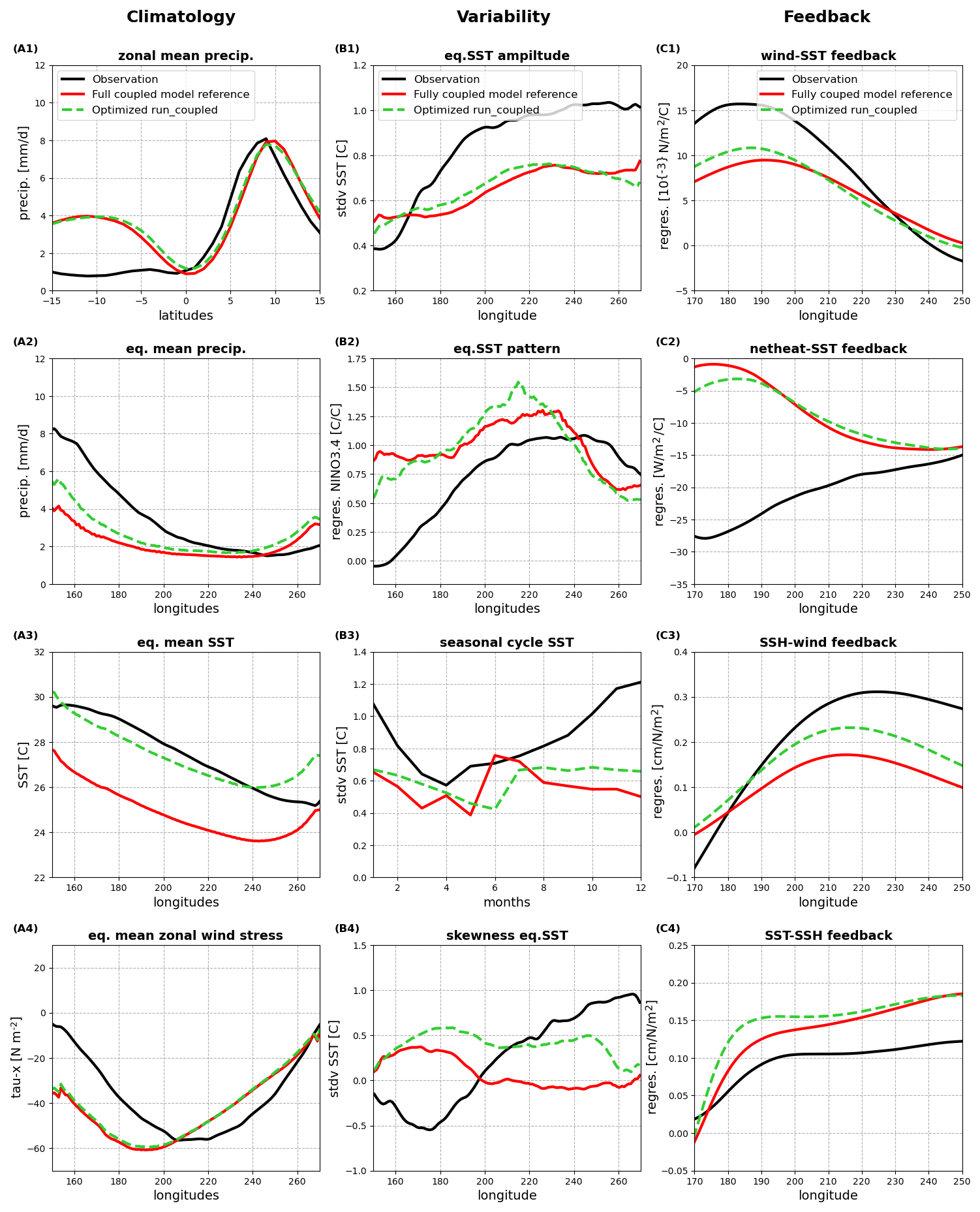
Figure 9 Comparison of ENSO metrics from the ICON XPP fully coupled reference simulation (“Fully coupled model reference”, red line), observations (“Observation”, black line), and the optimized coupled-model experiment (“Optimized run_coupled”, green dash line). The metrics are identical to those shown in Fig. 1.

Climatological precipitation metrics show mixed outcomes. The meridional precipitation structure (Fig. 9A1) remains largely unchanged from the reference run, indicating limited progress in correcting the double ITCZ bias. Zonal precipitation bias (Fig. 9A2) is slightly reduced over the western Pacific (150–200° E), though substantial errors persist further east. In contrast, climatological SST (Fig. 9A3) exhibits a moderate reduction in the cold tongue bias across the central-to-eastern equatorial Pacific, representing a partial improvement achieved through the optimization. However, zonal wind stress (Fig. 9A4) shows minimal change, with the optimized simulation closely resembling the reference case.

For ENSO variability, some aspects show improvement while others remain deficient. The amplitude of SST anomalies (Fig. 9B1) increases toward observed levels, although the overall variance remains underestimated. Seasonal phase-locking (Fig. 9B3) shows improvement, particularly during boreal summer, with a reduction of the unrealistic early peak seen in the reference run. The spatial structure of ENSO-related SST anomalies (Fig. 9B2) displays modest improvement between 150 and 200° E, while skewness (Fig. 9B4) becomes more realistic in the eastern Pacific (200–260° E) but degrades in the central region, suggesting regional trade-offs associated with the atmospheric-only tuning.

Feedback processes display a similar pattern of selective improvement. The Bjerknes feedback (Fig. 9C1) and the thermal damping feedback (Fig. 9C2) show moderate enhancement in the central Pacific (170–200° E). The wind–thermocline feedback (Fig. 9C3) exhibits the clearest improvement, indicating stronger coupling between wind stress and subsurface variability. However, the thermocline–SST feedback (Fig. 9C4) remains largely unchanged, highlighting that key oceanic processes are still inadequately represented despite the atmospheric parameter tuning.

In summary, the coupled-model tuning yields valuable improvements in SST climatology, ENSO amplitude, seasonal phase-locking, and air–sea coupling feedbacks. However, persistent deficiencies in precipitation structure, wind stress patterns, and oceanic feedbacks highlight the need for additional tuning to fully capture the dynamics of ENSO within the coupled system.

5.3 Comparison of ENSO metrics between optimized run and CMIP6 results

Figure 10 summarizes the ICON XPP model's performance across four categories of ENSO metrics – tropical climatology, ENSO characteristics, feedbacks, and teleconnections – comparing the fully coupled reference run, the optimized coupled-model experiment, and a high-resolution ICON configuration (Müller et al., 2025b). The CMIP6 multi-model ensemble distribution (light blue box, Planton et al., 2021) is also shown for context. In these normalized metrics, a lower value indicates smaller deviation from observations and therefore better performance, with values below zero representing improvement relative to the CMIP6 ensemble mean. This comparison provides a quantitative benchmark for assessing how the ICON XPP configurations perform relative to state-of-the-art CMIP6 models.

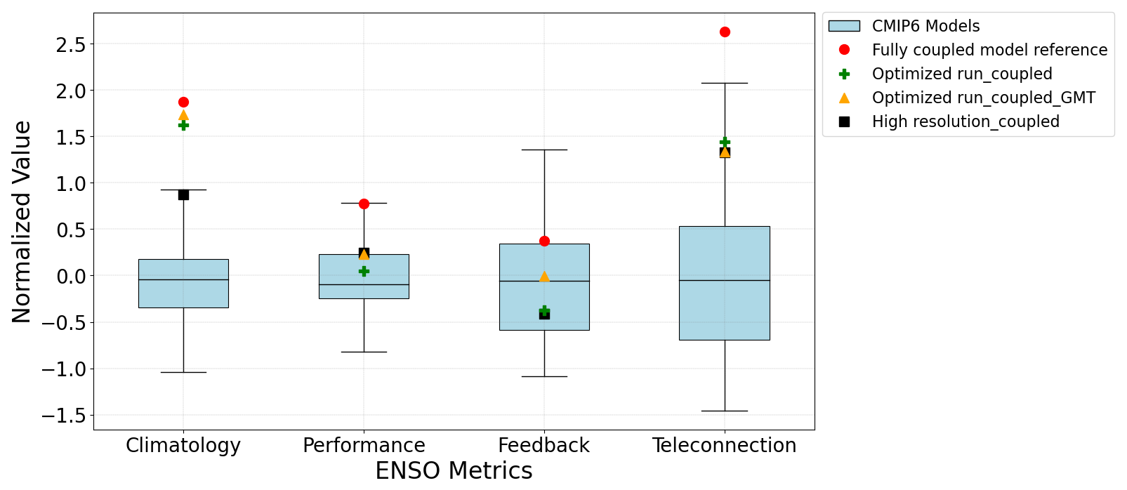
Figure 10 Summary of ICON XPP model performance across different categories of ENSO metrics – tropical climatology, ENSO characteristics, feedbacks, and teleconnections – comparing the fully coupled reference run (“Fully coupled model reference”, red point), optimized coupled-model experiment (“Optimized run_coupled”, green cross), fully coupled high resolution run for ICON XPP model (“high resolution_coupled”, black rectangle), optimized coupled-model experiment with global mean temperature (GMT) correction (“Optimized run_coupled_GMT”, yellow triangle). The CMIP6 distribution is shown as a boxplot with the box representing the interquartile range (25th–75th percentile), the central line indicating the median, and whiskers showing the full model spread (minimum to maximum). See Planton et al. (2021) for detailed definitions of all ENSO metrics and different categories. The ENSO metrics values for observation are −2.43, −1.77, −2.27, and −6.82 for Climatology, Performance, Feedback, and Teleconnection, respectively.

Despite showing limited improvement in overall tropical climatology biases, as demonstrated by persistent precipitation errors, the optimized fully coupled run achieves measurable advancements in key aspects of ENSO performance and feedback processes relative to the reference simulation. Among the four ENSO metric categories, the most notable progress occurs in the feedback metrics, where the optimized ICON XPP outperforms the CMIP6 multi-model mean. However, for the other categories – tropical climatology, ENSO characteristics, and teleconnections – the ICON XPP simulations still exhibit substantial room for improvement to reach or exceed the CMIP6 ensemble average. Importantly, teleconnection metrics were not explicitly included in the optimization process; their modest improvement therefore represents an emergent response to ENSO-targeted tuning, suggesting that systematic parameter optimization can enhance broader model performance beyond the specific metrics included in the cost function.

In addition to evaluating the reference and optimized runs, Fig. 10 further presents the results from an ICON XPP higher-resolving configuration (80 km atmosphere/20 km ocean), as described in Müller et al. (2025b). Previous studies have consistently demonstrated that increasing model resolution generally leads to improved ENSO simulation performance, including more realistic representations of ocean-atmosphere feedback processes, SST patterns, and ENSO variability (Shaffrey et al., 2009; Roberts et al., 2018). Comparing the high-resolution configuration to the low-resolution reference run confirms that increasing resolution will also substantially improve ENSO Metrics in ICON XPP Earth System Model, especially in tropical climatology and ENSO teleconnection simulations. Most notably, the impact of our optimization result at standard resolution is comparable in magnitude to the improvement gained from doubling model resolution. This equivalence – observed across several ENSO categories – demonstrates the power of systematic linear sensitivity-based tuning as a systematic linear method for improving climate model performance. Given that our method matches the effectiveness of a much more resource-intensive high-resolution setup, applying this tuning strategy in high-resolution simulations has the potential to yield even greater performance gains. Thus, the combination of systematic parameter tuning and increased resolution represents a potential path forward for advancing ENSO realism in coupled climate models.

5.4 Global mean temperature bias and model stability adjustment

While the primary objective of this study is to optimize ENSO-related processes, an important unintended consequence emerged during coupled model simulations. Specifically, the optimized fully coupled run (“Optimized run_coupled”) – derived from ENSO-focused parameter tuning – exhibits an unrealistic global mean surface warming, with a global mean 2 m temperature bias reaching +1.58 °C and local maxima up to +15.65 °C. This excessive warming is not present in the reference fully coupled simulation, which remains closer to observed climatology.

This warming bias is attributed to a destabilization of turbulent mixing processes, particularly those governed by the heat and momentum mixing parameters (f_theta_limit_fraction and f_tau_limit_fraction), which regulate limiting thresholds in the ICON turbulence scheme under strongly stratified conditions. These parameters influence the reduction of turbulent exchange coefficients in stable layers, helping to prevent excessive vertical mixing that could otherwise lead to unrealistic near-surface warming (Dipankar et al., 2015; Heinze et al., 2017). In a revised fully coupled experiment, we addressed this issue by reducing both of these parameters to 0.1. The resulting simulation shows that global mean warming is effectively suppressed (global mean bias reduced to +0.09 °C), while ENSO-related metrics (“Optimized run_coupled_GMT”, yellow triangle in Fig. 10) remained largely unchanged and stable compared to the original optimized run.

These findings underscore a critical lesson: although targeted tuning of ENSO metrics can lead to meaningful improvements in tropical Pacific variability, it may simultaneously destabilize other components of the global climate system if broader metrics (e.g., global mean temperature, AMOC index) are excluded from the cost function. Therefore, to achieve both regional and global fidelity, future tuning efforts – especially within coupled models – should include constraints based on large-scale climate indicators. This example demonstrates that our linear sensitivity optimization is a powerful tool, but one that benefits from holistic design. Including global-scale constraints will be a crucial step forward in enhancing the physical realism and overall climate consistency of optimized Earth System Models like ICON XPP.

6 Summary and discussion

The ENSO phenomenon has distinct impact on global climate patterns and extreme weather events. Therefore, accurate model representation of ENSO phenomenon is paramount for climate research and prediction. By leveraging the comprehensive ENSO Metrics Package (Planton et al., 2021), this study introduces a systematic, linear sensitivity-based optimization method to enhance ENSO representation in the ICON XPP Earth System Model. The foundation of the optimization method is a targeted ensemble of experiments of span the hyperspace of model parameters. Here we consider 21 atmosphere parameters that are related to cloud cover, microphysics and turbulence parameterization. Based on these experiments, the optimization procedure estimates the sensitivity of the ENSO metrics to the parameters and generates the best possible parameter combination for the optimization experiments.

The atmosphere-only optimization experiments demonstrate the effectiveness of the linear sensitivity-based tuning approach in improving ENSO-related performance in ICON XPP. The resulting optimized simulation achieved a ∼30 % reduction in the ENSO metrics cost function (from 1.0 to 0.73), highlighting significant improvement relative to the reference run. Physically, the optimized parameters lead to meaningful corrections in several key biases, including a reduced double ITCZ pattern in meridional precipitation, improved zonal wind stress, and enhanced representation of the Bjerknes and thermal damping feedbacks. Interestingly, although the optimization targeted only ENSO-specific metrics, broader improvements are observed in global precipitation and wind stress patterns. Hence, the atmosphere-only results confirm that systematic, sensitivity-guided parameter tuning can effectively reduce model biases.

Following the atmosphere-only optimization, we conduct a second stage of tuning with fully coupled ICON XPP simulations, repeating the perturbation experiments for the selected parameters. Then, we recalculate parameter sensitivities within the coupled system and apply the same linear sensitivity-based optimization framework. The improvement of ENSO simulations by our optimized method is comparable with the effect of increase resolution in model, and the ENSO feedback enhancements now position the optimized ICON XPP performance better than the average CMIP6 model feedback metrics. Specifically, the optimization yields targeted improvements in several critical ENSO metrics, such as the climatological SST distribution, ENSO amplitude, seasonality, and the wind–thermocline feedback. However, certain ENSO-related characteristics – such as precipitation seasonality, SST variance, and thermocline–SST feedback – remain largely unaffected by atmospheric parameter changes. These limitations underscore the importance of extending systematic tuning strategies beyond the atmosphere, particularly toward ocean model parameters and background state biases.

An important insight emerges during fully coupled tuning: while optimizing for ENSO metrics improved regional performance, it inadvertently induces unrealistic global mean temperature (GMT) warming. This warming bias, with global mean 2-meter temperature exceeding observations by over 1.5 °C and maxima above 15 °C, is traced to destabilized vertical mixing due to insufficient constraints on turbulent damping in stably stratified layers. The issue is resolved by reducing the heat and momentum turbulence mixing parameters, restoring realistic GMT values while preserving ENSO improvements. This result underscores that ENSO-focused tuning alone may destabilize other components of the climate system if global metrics are excluded from the tuning process. In future applications, constraints such as global energy balance, AMOC strength, or GMT could be incorporated into the optimization framework to ensure broader physical consistency.

At the same time, we emphasize a key methodological limitation: the present framework relies on a first-order linear approximation of parameter sensitivities and therefore cannot fully represent higher-order nonlinear parameter interactions. This trade-off was chosen for computational feasibility in expensive coupled simulations. The fact that measurable ENSO improvements are obtained under this linear framework demonstrates its practical value for targeted, process-oriented tuning. Nevertheless, extending this work toward more comprehensive nonlinear optimization remains an important next step and will be pursued in future work.

In conclusion, this study demonstrates that our linear sensitivity-based optimization framework effectively identifies and tunes key atmospheric parameters, to improve representation of critical ENSO characteristics and feedback processes fidelity within the ICON XPP Earth System Model. With greater computational resources, the approach can be extended to multi-objective optimization that simultaneously targets ENSO metrics and large-scale climate constraints (e.g., tropical mean SST, global energy balance, AMOC, GMT), and to broader parameter spaces including ocean and sea-ice schemes. Doing this well will require a team effort that combines climate process expertise, numerical optimization and uncertainty quantification (e.g., ensemble design, regularization, and cross-validation against out-of-sample periods).