Benchmarking ozone stress parameterizations in CLM5: a global mechanistic assessment of thresholds and memory effects

Tropospheric ozone remains a critical but uncertain driver of terrestrial productivity loss, and land surface models (LSMs) diverge markedly in how they represent vegetation ozone stress. We conduct a global, mechanistically consistent evaluation of three prominent ozone stress parameterization schemes, Sitch, Lombardozzi, and Li, within the Community Land Model version 5 (CLM5). Using unified meteorological and ozone forcing from CAM-chem and GSWP3.1, we designed five experiments to isolate the roles of ozone flux threshold selection and response function form. The mixed experiments using thresholds and response functions derived from the Sitch and Lombardozzi schemes were implemented without additional recalibration, allowing structural sensitivities to be evaluated consistently within the Li framework. Model output is benchmarked against MODIS and FLUXNET gross primary production (GPP) across spatial gradients, biomes, and among plant functional types (PFTs). All parameterizations capture the ozone–induced reduction in GPP relative to the ozone-free baseline, but their accuracy varies widely. The Li scheme, featuring PFT-specific thresholds and separate nonlinear responses for photosynthesis and stomatal conductance, best agrees with observed GPP patterns across scales. In contrast, the Lombardozzi scheme produces much larger reductions in high-flux regions. Analysis reveals that the structures of ozone response functions and memory-decay mechanisms primarily determine improvements in GPP simulation. Our results support a shift toward ozone parameterizations that couple stomatal flux with canopy phenology, dynamic water constraints, and regionally calibrated thresholds. These findings provide a transferable framework for quantifying ozone–carbon coupling in LSMs and highlight priorities for improving terrestrial biosphere models under atmospheric change.

1 Introduction

Tropospheric ozone (O₃), a typical secondary pollutant primarily produced by photochemical reactions of anthropogenic precursors under solar radiation, has been shown to threaten human health, crop yields, and ecosystem functioning as near-surface concentrations increase (Agathokleous et al., 2020; Turnock et al., 2020; Feng et al., 2022; Achebak et al., 2024). Ecological and agronomic studies indicate that, compared with counting exceedances based on concentration thresholds such as the accumulated exposure over a threshold of 40 ppb (AOT40), whether vegetation is truly damaged depends more on the actual uptake of ozone through stomata and its accumulation over time (Emberson et al., 2018; Paoletti et al., 2022; Pleijel et al., 2022). This insight has driven a shift from concentration-based exposure metrics to cumulative flux dose and calls for process representations that more closely capture flux controls and temporal memory at leaf and canopy scales (Mills et al., 2011; Montes et al., 2021; Moura et al., 2023). Consequently, metrics and parameterization schemes grounded in stomatal ozone flux are essential for quantifying ozone–vegetation interactions across space and time. They provide the methodological foundation for integrated carbon flux assessment of ozone flux thresholds, cumulative dose, and response functions within the ecosystem for land surface models (Karlsson et al., 2007; Mills et al., 2011). In land surface models, the scientific rationale for adopting ozone-stress parameterizations is that ozone injury is not directly determined by ambient concentration alone, but by the amount of ozone entering leaves through stomata, the capacity of plants to detoxify or tolerate that flux, and the subsequent physiological downregulation of photosynthesis and stomatal conductance (Sitch et al., 2007). Without such process-based parameterizations, models either neglect an important atmospheric stressor or treat ozone exposure in a manner disconnected from canopy physiology, water limitation, phenology, and differences in plant functional type (Fuhrer, 1996). Therefore, ozone-stress parameterizations provide the necessary mechanistic bridge between atmospheric ozone forcing and terrestrial carbon-cycle responses, allowing land surface models to diagnose when ozone damage is triggered, how it accumulates over time, and how strongly it suppresses GPP across different ecosystems.

Sitch et al. (2007) first introduced a flux-based exposure assessment in the Met Office Surface Exchange Scheme Top-down Representation of Interactive Foliage and Flora Including Dynamics (MOSES-TRIFFID) model, with the predominant form being PODY (phytotoxic O₃ dose over a flux threshold of Y nmol O₃ m⁻² s⁻¹), which represents the time integral of ozone flux above a threshold and in the original implementation applied a single linear attenuation factor to scale both photosynthesis and stomatal conductance. Lombardozzi et al. (2013) treated cumulative uptake of O₃ (CUO) as a state variable in the Community Land Model version 5 (CLM5), first solving for an ozone-free state and then applying plant functional type-specific linear scalings to photosynthesis and stomatal conductance, while distinguishing sunlit and shaded leaves and introducing growing-season gating, leaf turnover, and longevity-related decay to limit unrealistic long-term accumulation. Li et al. (2024), also within CLM5, continued to base the parameterization scheme on above-threshold flux accumulation but selected an optimal ozone flux threshold in a data-driven manner and, from multiple candidate forms, identified the best response functions for photosynthesis and stomatal conductance for each plant functional type. These developments enable ozone stress to be embedded in ecosystem and land surface models in a flux-based manner, thereby creating a coherent linkage with assessments of the carbon and water cycles.

However, we still lack a systematic, comprehensive assessment of the performance of the Sitch, Lombardozzi, and Li ozone-stress parameterizations, and the relative strengths, weaknesses, and domains of applicability of these parameterizations remain unclear. Existing studies often evaluate under different model settings, ozone flux thresholds, and response function selections, and varying driving and validation data conditions, or test only a single (or two) parameterization scheme for ozone stress (Gong et al., 2020; Cao et al., 2024). The impact of ozone flux threshold setting, cumulative dose characterization, and response function morphology of the three parameterization schemes on carbon flux has not yet been quantified within a unified mechanistic framework. Therefore, it is difficult to objectively assess the superiority and applicability of these parameterization schemes across models with different spatiotemporal distributions, biomes, or vegetation types. Benefiting from the large-scale, assimilation-consistent Moderate Resolution Imaging Spectroradiometer (MODIS) gross primary production (GPP) (Running et al., 2004; Ma et al., 2024), the process-based and high-temporal-resolution FLUXNET site fluxes (Baldocchi et al., 2001; Pastorello et al., 2020), and spatiotemporally consistent ozone fields from chemical transport models (Lamarque et al., 2012), we are now able to evaluate, within a single mechanistic framework, a no-ozone baseline together with established and modified parameterization schemes across scales, regions, and vegetation types.

Building on these advances and the above modeling needs, we here address the research gap by asking: (1) how do the Sitch et al. (2007), Lombardozzi et al. (2015), and Li et al. (2024) ozone-stress schemes differ in their impacts on GPP when evaluated under consistent conditions? (2) To what extent do differences in ozone flux threshold choices versus response function forms contribute to the variability in simulated ozone damage? (3) Which scheme best reproduces observed GPP patterns across regions and plant functional types? To answer these questions, we modify and compare multiple ozone-stress parameterization schemes in CLM5 around three core elements: ozone flux thresholds, cumulative dose, and response functions. Using simulated ozone and meteorological reanalysis as forcings, and coupling them with the land model's native resistance network and canopy stratification, we comprehensively evaluate how alternative ozone flux threshold settings and response functional forms scale photosynthesis and stomatal conductance. In parallel, MODIS GPP and FLUXNET flux observations serve as constraints and independent validation to test robustness across plant functional types and regions at multiple scales. By juxtaposing a no-ozone baseline, representative existing parameterization schemes, and modified parameterization schemes, we aim to clarify the dominant contributions of ozone flux threshold selection and response-function uncertainty to the outcomes, thereby providing diagnostic, traceable modeling baselines and data evidence for studies that couple ozone with the carbon and water cycles. Notably, the mixed-parameterization experiments using thresholds and response functions derived from the Sitch and Lombardozzi schemes were not recalibrated within the Li framework and should therefore be interpreted primarily as structural-sensitivity experiments.

2 Materials and methods

2.1 Model platform and experimental setup

We evaluate the impact of ozone stress on vegetation productivity within the offline framework of the Community Terrestrial Systems Model version 5.3.075 (CTSM 5.3.075) (Lawrence et al., 2019). The land surface model uses the CLM5 photosynthesis and stomatal coupling scheme (Farquhar–Collatz photosynthesis and Medlyn stomatal conductance) and, on this basis, incorporates alternative ozone stress parameterizations to conduct comparative experiments (see Sect. 2.2) (Farquhar et al., 1980; Collatz et al., 1991, 1992; Medlyn et al., 2011). The model uses the I2000Clm50Sp compset (prescribed vegetation with the biogeochemical module disabled), so ozone acts solely as an external stressor on land-surface physiological processes and does not interact with the atmosphere through coupled feedbacks.

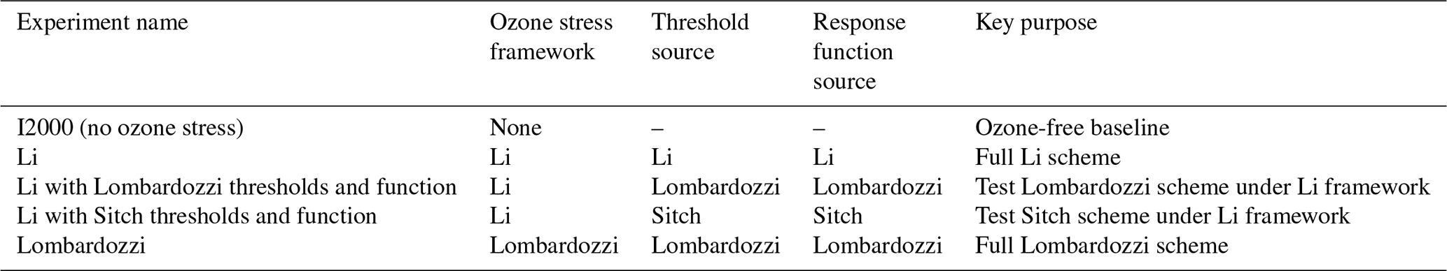
The numerical experiments use a global latitude–longitude grid (1.895° latitude by 2.5° longitude) with a 30 min time step. The simulation spans 30 years by cycling the atmospheric forcing and surface ozone fields from 2005 to 2014 three times. The first 10 years are discarded as spin-up, and only steady-state statistics from the final 20 years are analyzed. The control and sensitivity experiments include a no-ozone baseline (I2000), the Li parameterization, the Li with Lombardozzi thresholds and function, the Li with Sitch thresholds and function, and the Lombardozzi parameterization (Table 1). All other physical and physiological parameters are held constant to ensure that any differences are attributable solely to the ozone process.

Table 1 Summary of model experiments used in this study.

The atmospheric forcing is taken from the Global Soil Wetness Project (GSWP3.1), which provides three-hourly reanalysis fields at 0.5°×0.5° resolution for 2005–2014, including near-surface air temperature, specific humidity, wind speed, surface pressure, incoming longwave and shortwave radiation, sunshine duration, and precipitation (Dirmeyer, 2011). Vegetation structure follows prescribed contemporary distributions and parameters, such as leaf area index (LAI) and canopy height, derived from MODIS and held constant across years. All forcing and initial datasets, including the year-2000 atmospheric CO₂ concentration and the nitrogen and aerosol deposition fields, are taken from the standard datasets provided with CTSM 5.3.075.

Ozone forcing was obtained from our CAM-chem version 6 simulations of hourly near-surface ozone concentrations for 2005–2014 at 0.9°×1.25° horizontal resolution with 32 vertical levels (Tilmes et al., 2019; Emmons et al., 2020). Further details of the CAM-chem simulation configuration and experimental design are described in another of our studies (Murray et al., 2026). CAM-chem was run in specified-dynamics mode and employed the Model for Ozone and Related Chemical Tracers troposphere and stratosphere mechanism version 1 (MOZART-TS1) (Granier et al., 2019). Anthropogenic, biogenic, and biomass-burning emissions were taken from the Community Emissions Data System (CEDS), the Model of Emissions of Gases and Aerosols from Nature (MEGAN), and a standard fire emissions inventory (QFED), respectively (Wiedinmyer et al., 2011; Guenther et al., 2012; Darmenov and da Silva, 2015). Air temperature (T) together with the zonal (u) and meridional (v) wind components are taken from the Modern-Era Retrospective analysis for Research and Applications, Version 2 (MERRA-2) reanalysis (Gelaro et al., 2017).

To provide an independent comparison with the model results, we use the monthly MODIS GPP (MOD17A2) product at 0.05° resolution to assess consistency with our simulated results for the same period (Zhao et al., 2005). At the same time, we incorporate site-level FLUXNET flux observations (Pastorello et al., 2020), apply quality control and gap-filling to the site monthly time series, and pair the observations with the model outputs station by station and month by month, using only samples that are fully collocated in space and time as the observational benchmark for the evaluation.

2.2 Calculation of ozone flux and cumulative dose

2.2.1 Calculation principle of Sitch

Sitch et al. (2007) described ozone suppression of instantaneous net photosynthesis in MOSES-TRIFFID using the concept of accumulated ozone flux above a threshold (POD_Y, mmol m⁻²). They first compute the instantaneous stomatal ozone flux $F_{{\mathrm{O}}_{\mathrm{3}}}$ (nmol m⁻² s⁻¹), then integrate the above-threshold portion over time to obtain POD_Y, from which a photosynthetic inhibition factor is defined. At each time step, the instantaneous ozone flux $F_{{\mathrm{O}}_{\mathrm{3}},t}$ is calculated (in a form analogous to Ohm's law) and can be written as:

$$\begin{array}{}\text{(1)}& F_{{\mathrm{O}}_{\mathrm{3}},t}={\displaystyle \frac{c_{{\mathrm{O}}_{\mathrm{3}},t}}{r_{\mathrm{b}}+r_{\mathrm{a}}+\frac{\mathrm{1}}{\mathrm{1.67}{g}_{\mathrm{s}}}}},\end{array}$$

where $c_{{\mathrm{O}}_{\mathrm{3}},t}$ is the molar concentration of ozone (nmol m⁻³), t denotes the model time step. r_b+r_a is the sum of the quasi-laminar boundary-layer resistance and the aerodynamic resistance over the leaf surface (s m⁻¹), g_s is the leaf conductance to water vapor (m s⁻¹), and 1.67 is the ratio of the diffusion resistance of ozone to that of water vapor.

For each time step t, the ozone flux above the threshold is defined:

$$\begin{array}{}\text{(2)}& F_{{\mathrm{O}}_{\mathrm{3}},t}^{>}\max \left(F_{{\mathrm{O}}_{\mathrm{3}},t}-Y,\mathrm{0}\right),\end{array}$$

where Y is the vegetation-type-dependent critical ozone flux threshold.

Within a given accumulation time window, the ozone flux above the threshold in Eq. (2) is accumulated over time to obtain the total above-threshold dose:

$$\begin{array}{}\text{(3)}& {\mathrm{POD}}_Y=\sum _{t=\mathrm{1}}^T{F}_{{\mathrm{O}}_{\mathrm{3}},t}^{>}\mathrm{\Delta }t,\end{array}$$

where Δt is the length of the time step (s).

$$\begin{array}{}\text{(4)}& f=\mathrm{1}-a\cdot {\mathrm{POD}}_Y,\end{array}$$

where a is a vegetation-type-specific sensitivity parameter. Net photosynthesis is modified to $A=A_{\mathrm{0}}(\mathrm{1}-a\cdot {\mathrm{POD}}_Y)$, where A₀ is the photosynthetic rate in the absence of O₃. Similarly, stomatal conductance is modified to $g_{\mathrm{s}}=g_{{\mathrm{s}}_{\mathrm{0}}}(\mathrm{1}-a\cdot {\mathrm{POD}}_Y)$, where $g_{{\mathrm{s}}_{\mathrm{0}}}$ is the stomatal conductance in the absence of O₃.

Because g_s is linearly related to the photosynthetic rate, combining Eqs. (1) to (3) with the conductance relationship yields a quadratic equation in g_s, which can be solved analytically.

2.2.2 Calculation principle of Lombardozzi

Lombardozzi et al. (2015) accumulated the stomatal ozone flux exceeding the threshold over time to obtain the cumulative uptake (CUO, mmol m⁻²), and used a linear response factor to directly scale net photosynthesis and leaf stomatal conductance in the absence of O₃. For a given flux threshold Y specific to the plant functional type (PFT) and a time step Δt, within a prescribed accumulation window, we define:

$$\begin{array}{}\text{(5)}& \mathrm{CUO}=\sum _{t=\mathrm{1}}^T\max \left(F_{{\mathrm{O}}_{\mathrm{3}},t}-Y,\mathrm{0}\right)\mathrm{\Delta }t,\end{array}$$

(κ is the conversion factor from nmol to mmol.)

Subsequently, PFT-specific linear response factors are used to scale ozone-free photosynthesis and conductance:

$$\begin{array}{}\text{(6)}& {\displaystyle }& {\displaystyle }A=A_{\mathrm{0}}(\mathrm{1}-b\cdot \mathrm{CUO}),\text{(7)}& {\displaystyle }& {\displaystyle }{g}_{\mathrm{s}}=g_{{\mathrm{s}}_{\mathrm{0}}}(\mathrm{1}-c\cdot \mathrm{CUO}),\end{array}$$

where b and c are regression coefficients specific to PFT.

2.2.3 Calculation principle of Li

Building on the framework mentioned above, Li et al. (2024) represented ozone stress as the cumulative ozone flux above a threshold over time and accounted for damage decay due to leaf turnover. The cumulative dose POD_Y is computed recursively at each time step t as:

$$\begin{array}{}\text{(8)}& {\mathrm{POD}}_{Y,t}=\left(\mathrm{1}-{\mathit{\delta }}_t\right){\mathrm{POD}}_{Y,t-\mathrm{1}}+F_{{\mathrm{O}}_{\mathrm{3}},t}^{>}\mathrm{\Delta }t,\end{array}$$

where POD${}_{Y,t-\mathrm{1}}$, and POD_Y,t denote the cumulative above-threshold dose at time steps t−1 and t, respectively.

δ_t is the fraction of decay caused by leaf turnover or abscission and is calculated as follows:

$$\begin{array}{}\text{(9)}& {\mathit{\delta }}_t=\mathrm{1}-\exp \left(-{\displaystyle \frac{\mathrm{\Delta }{\mathrm{LAI}}_t}{L_{\mathrm{leaf}}}}\right)\end{array}$$

where L_leaf is the leaf lifetime (years), and LAI_t−1 and LAI_t are the leaf area index at time steps t−1 and t, respectively.

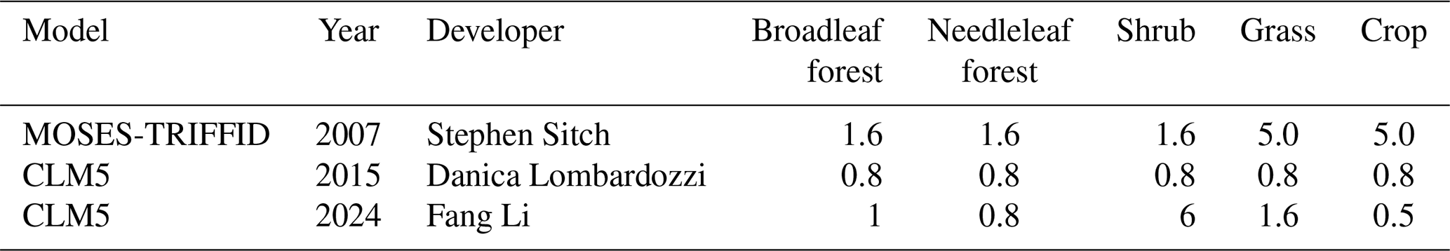
Table 2 Ozone flux thresholds Y for different PFTs in the three ozone stress parameterizations.

After obtaining the growing season cumulative dose POD_Y, dimensionless response factors for net photosynthesis and stomatal conductance are constructed as:

$$\begin{array}{}\text{(10)}& {\displaystyle }& {\displaystyle }{f}_{\mathrm{A}}=h_{\mathrm{A}}\left({\mathrm{POD}}_Y\right),\text{(11)}& {\displaystyle }& {\displaystyle }{f}_{\mathrm{g}}=h_{\mathrm{g}}\left({\mathrm{POD}}_Y\right),\end{array}$$

where h_A and h_g are inhibition functions for photosynthesis and conductance (with values between 0 and 1).

The three approaches differ fundamentally in how thresholds are prescribed and how response functions are formulated (Table 2). Sitch uses ozone flux above the threshold, expressed as POD_Y, as the core quantity. In this parameterization scheme, the ozone flux thresholds are prescribed by PFT, and a single linear inhibition factor is applied to scale photosynthesis and stomatal conductance simultaneously (both the ozone flux thresholds and the response functions involve assumptions). Lombardozzi instead integrates over time the part of the flux that exceeds 0.8 nmol m⁻² s⁻¹ to obtain CUO, uses a fixed threshold for all PFTs, and applies separate linear scalings of photosynthesis and conductance based on regression coefficients fitted for each PFT. Li adopts a data-driven approach to selecting the optimal threshold Y and uses POD_Y as the cumulative quantity. For the response functions, this approach no longer restricts the form to linearity; instead, it selects, for each PFT, the best form among several candidates (linear, exponential, logarithmic, etc.) based on statistical criteria, and then applies separate multiplicative scalings to photosynthesis and conductance.

Compared with Sitch, Lombardozzi first represents ozone damage as a continuously updated state variable by computing ozone-free photosynthesis and stomatal conductance within the model, and then applies scaling based on this. Second, the effects of ozone on photosynthesis and stomatal conductance are treated in a decoupled manner, with separate ozone factors applied to each process, thereby allowing the asynchronous responses of photosynthesis and conductance to ozone commonly observed in the field (Wittig et al., 2007; Lombardozzi et al., 2013). Third, at the implementation level, the parameterization is refined to canopy radiation layers, with ozone uptake calculated and accumulated separately for sunlit and shaded leaves. Finally, growing-season gating and leaf-turnover effects are introduced, so that damage accumulates only during the growing season (diagnosed using a leaf area index threshold), and a healing offset is applied to newly emerged leaves, while evergreen leaves receive a decay term based on their lifetime.

Compared with Lombardozzi, Li retains the two-stage structure of flux accumulation and physiological scaling but provides greater detail for each component. Second, the flux calculation still relies on the native resistance chain and meteorological forcing in the land surface model, updates the ratio of diffusion resistances between ozone and water vapor, and uses the internal model time-scale parameters consistently in both time integration and the conversion based on leaf lifetime. Finally, for the physiological representation of the cumulative dose, the parameterization scheme continues to accumulate dose separately for sunlit and shaded leaves, accumulates dose only during daytime when vegetation effectively absorbs solar radiation, and sets leaf area index thresholds by plant functional type, with long-term memory controlled through two mechanisms, namely lifetime decay of leaves in evergreen vegetation and phenological replacement of leaves in deciduous vegetation.

2.3 Model evaluation

To quantitatively evaluate how well each ozone stress parameterization reproduces the observations, we use complementary metrics including correlation, agreement in magnitude, and error amplitude. We perform statistical analysis at different temporal aggregation levels and across different PFTs. All statistics are based on strictly paired samples, using only records for which observations and simulations are available at the same site and time step. The units of the metrics follow those of the variable being evaluated.

1. Root mean square error (RMSE): it measures the overall magnitude error between simulations and observations, is non-negative, and smaller values indicate better performance (Zhou et al., 2025a):

   $$\begin{array}{}\text{(12)}& \mathrm{RMSE}=\sqrt{{\displaystyle \frac{\mathrm{1}}{N}}\sum _{i=\mathrm{1}}^N{\left(P_i-O_i\right)}^{\mathrm{2}}},\end{array}$$

   where P_i and O_i are the simulated and observed values of the ith paired sample, respectively, and N is the number of paired samples.

2. Relative bias: it is used to describe the bias between simulations and observations or between simulations and the no-ozone-stress case (Lamarque et al., 2013):

   $$\begin{array}{}\text{(13)}& B_{\mathit{\%}}={\displaystyle \frac{\stackrel{\mathrm{‾}}{P}-\stackrel{\mathrm{‾}}{O}}{\stackrel{\mathrm{‾}}{O}}}\times \mathrm{100}\mathit{\%},\end{array}$$

   where $\stackrel{\mathrm{‾}}{P}$ and $\stackrel{\mathrm{‾}}{O}$ are the sample means of prediction and observation.

3. Pearson correlation coefficient (r): it measures the temporal phase consistency between simulations and observations, takes values in [−1, 1], and values closer to 1 indicate stronger correlation (Zhou et al., 2025b):

   $$\begin{array}{}\text{(14)}& r={\displaystyle \frac{\mathrm{cov}(P,O)}{{\mathit{\sigma }}_{\mathrm{P}}{\mathit{\sigma }}_{\mathrm{O}}}},\end{array}$$

   where σ_P and σ_O are the sample standard deviations, and cov(P, O) is the covariance between the simulated values P and the observed values O.

4. Normalized standard deviation (NSD): It is used to characterize the ability to reproduce the variability (amplitude) and is defined as the ratio of the standard deviation of simulations to that of observations (Taylor, 2001):

   $$\begin{array}{}\text{(15)}& \mathrm{NSD}={\displaystyle \frac{{\mathit{\sigma }}_{\mathrm{P}}}{{\mathit{\sigma }}_{\mathrm{O}}}}.\end{array}$$

   NSD = 1 indicates that the simulation variance is consistent with the observed variance, and NSD < 1 indicates attenuated variance.

5. Nash–Sutcliffe efficiency (NSE): it measures the degree of improvement of the simulations relative to using the observational mean as a naive model. It has a theoretical range from −∞ to 1, and values closer to 1 indicate better performance (Nash and Sutcliffe, 1970):

   $$\begin{array}{}\text{(16)}& \mathrm{NSE}=\mathrm{1}-{\displaystyle \frac{\sum _{i=\mathrm{1}}^N{\left(P_i-O_i\right)}^{\mathrm{2}}}{\sum _{i=\mathrm{1}}^N{\left(O_i-\stackrel{\mathrm{‾}}{O}\right)}^{\mathrm{2}}}},\end{array}$$

   when NSE = 0, the performance is equivalent to predicting a constant value $\stackrel{\mathrm{‾}}{O}$; and NSE < 0 indicates performance worse than this naive benchmark.

3 Results

3.1 Spatial evaluation and verification of ozone stress parameterization schemes

To quantitatively compare the impacts of different ozone stress parameterizations on land surface productivity, Fig. 1 presents the spatial distribution of the ten-year mean GPP and its zonal mean from 2005 to 2014. This includes the no ozone case (Fig. 1a), the Li parameterization (Fig. 1b), the Li parameterization combined with the threshold and response function sets of Lombardozzi and Sitch (Fig. 1c and d), the Lombardozzi parameterization (Fig. 1e), and the GPP from the MODIS satellite product (Fig. 1f). Compared with the MODIS observations (Fig. 1f), the no ozone case (Fig. 1a) shows pronounced overestimation of GPP in tropical regions, particularly in humid low-latitude ecosystems, indicating that neglecting ozone stress can substantially exaggerate tropical productivity. Compared with Fig. 1a, all parameterizations that include ozone show a systematic suppression of GPP and exhibit pronounced heterogeneity, with particularly low GPP values in humid tropical regions. The zonal-mean curves show that the peak values at the equator in the ozone-parameterized cases are clearly lower than in the no-ozone case, indicating that tropical regions are more sensitive to ozone stress. Among the different parameterizations, the Li parameterization scheme and its combinations with the Lombardozzi and Sitch thresholds and functions (Fig. 1b–d) are closer to MODIS (Fig. 1f) in terms of zonal gradients and tropical contrast, whereas the Lombardozzi parameterization scheme (Fig. 1e) produces lower GPP in the tropics, which enlarges the deviations from observations in these regions.

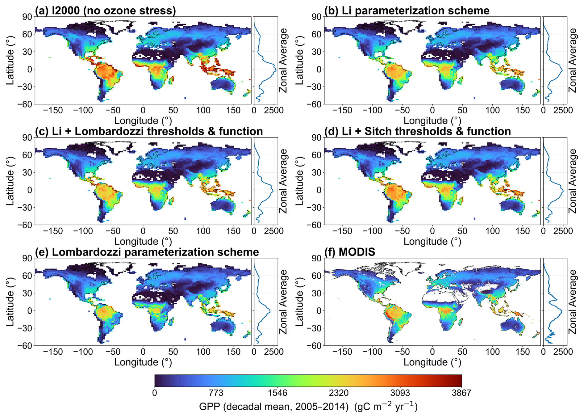
Figure 1 Decadal-mean (2005–2014) gross primary production (GPP) maps and zonal-mean profiles for (a) I2000 (no ozone stress), (b) Li, (c) Li with Lombardozzi thresholds and function, (d) Li with Sitch thresholds and function, (e) Lombardozzi, and (f) MODIS.

To test the ability of each parameterization scheme to reproduce the observations, Fig. 2 shows the spatial distribution of station-based RMSE of monthly GPP relative to FLUXNET and the corresponding zonal RMSE aggregated in 5° latitude bands. The figure shows that, across all five simulations and the MODIS product (Fig. 2a–f), RMSE is relatively low at high northern latitudes, whereas in the mid-latitudes the complexity of vegetation types leads to bands of abnormally high RMSE values. The high-resolution MODIS product has fewer extremely high values, indicating biases due to insufficient spatial resolution. Compared with FLUXNET, the no-ozone case (Fig. 2a) exhibits relatively large RMSE values in central African regions, reflecting pronounced overestimation under humid tropical conditions. However, at some stations in the middle and high latitudes, the no ozone case still shows lower RMSE values than the ozone-stress parameterization schemes. It is noteworthy that, compared with Fig. 2a (no ozone case), the Li parameterization and its combinations with the Lombardozzi and Sitch thresholds and functions (Fig. 2b–d) show some degree of improvement at different latitudes, indicating that optimal threshold settings for different PFTs (as in Li's scheme) reduce errors compared to using a single fixed threshold. The Lombardozzi parameterization (Fig. 2e) retains relatively large errors in some low-latitude bands. The zonal curves show that, compared with the no-ozone case, the overall variation in the ozone parameterizations is not very pronounced, but the inclusion of ozone stress yields a considerable reduction in errors in the tropics. The RMSE results for MODIS (Fig. 2f) provide some support for the reliability of the five simulations, as MODIS and FLUXNET show broadly similar RMSE patterns.

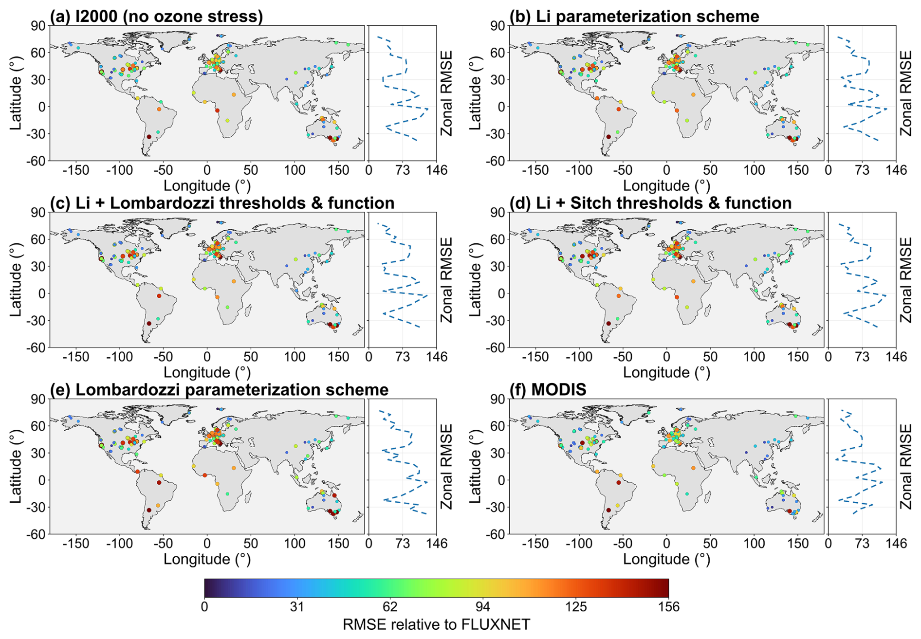
Figure 2 Spatial patterns and zonal-mean RMSE of site-level monthly GPP relative to FLUXNET for 2005–2014 for (a) I2000 (no ozone stress), (b) Li, (c) Li with Lombardozzi thresholds and function, (d) Li with Sitch thresholds and function, (e) Lombardozzi, and (f) MODIS.

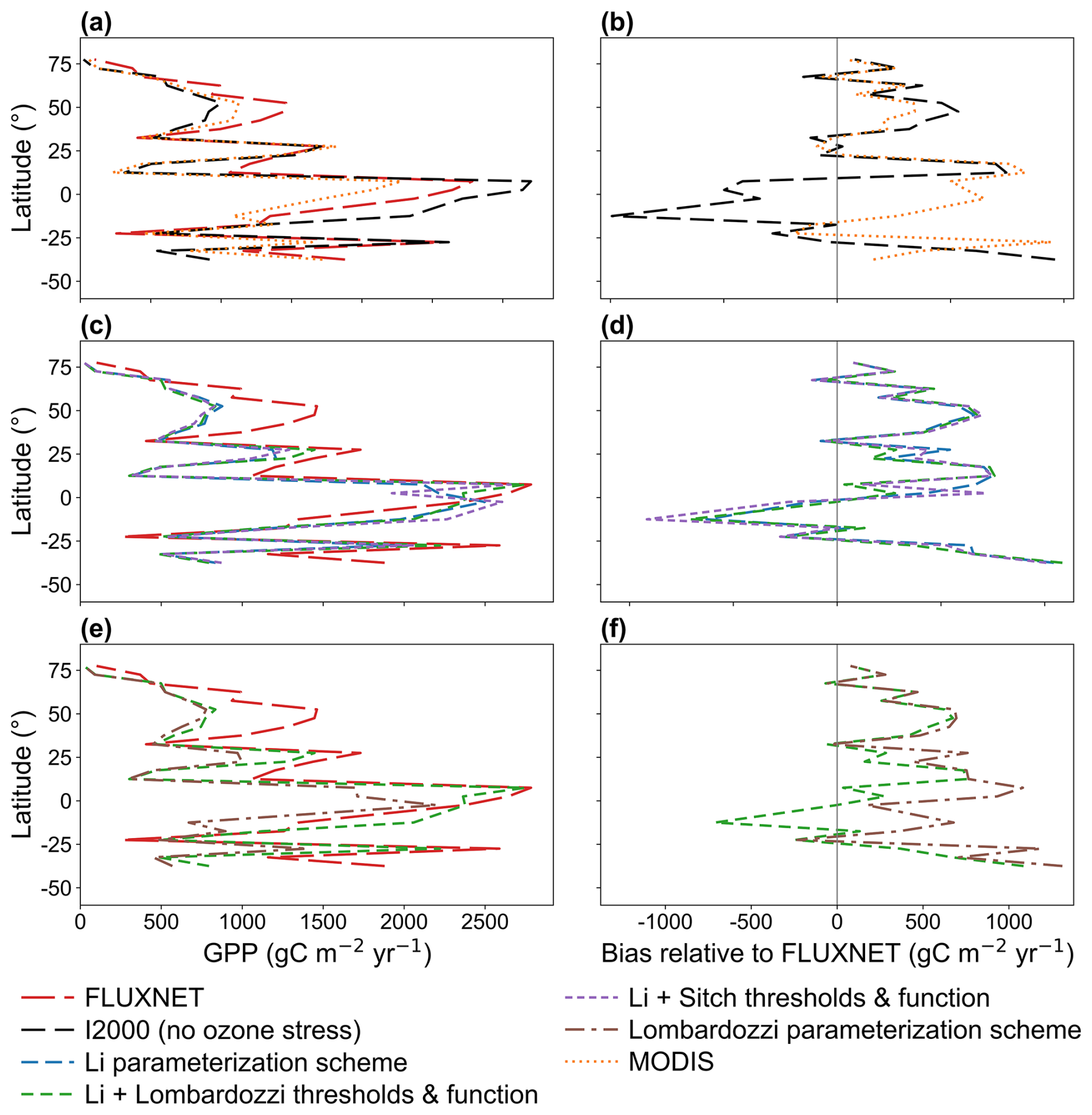
Figure 3 Zonal-mean profiles of GPP and zonal-mean bias relative to FLUXNET for 2005–2014. (a) Zonal-mean GPP from FLUXNET, I2000 (no ozone stress), and MODIS; (b) corresponding zonal-mean biases; (c) zonal-mean GPP from Li, Li with Lombardozzi thresholds and function, and Li with Sitch thresholds and function; (d) corresponding zonal-mean biases; (e) zonal-mean GPP from Li with Lombardozzi thresholds and function and from Lombardozzi; (f) corresponding zonal-mean biases.

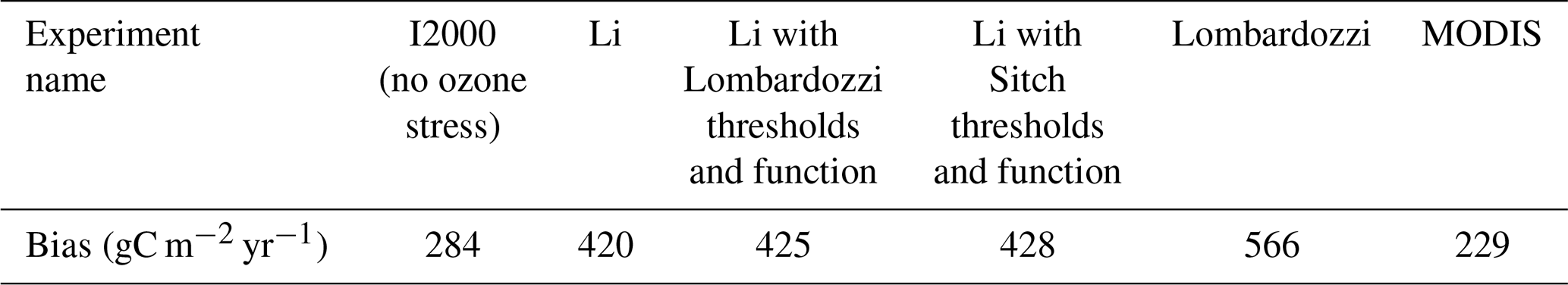
To characterize the consistency between the model and the observations along the zonal gradient, Fig. 3 shows zonal profiles of GPP aggregated in 5° latitude bands (left panels) and their zonal biases relative to FLUXNET (right panels). Figure 3a and 3 provides the baseline comparison: the no-ozone case generally underestimates GPP in the midlatitudes of the Northern Hemisphere (around 20–50° N) and also shows substantial underestimation in the midlatitudes of the Southern Hemisphere, but exhibits pronounced overestimation in the tropics. MODIS as a whole tends to underestimate GPP (relative to FLUXNET), particularly at low latitudes and in the Southern Hemisphere midlatitudes. Only a few latitude bands show slight overestimation by MODIS, which is consistent with the findings of Wild et al. (2022). The bias statistics further support these zonal characteristics (Table 3). The no-ozone case shows an overall annual mean bias of 284 g C m⁻² yr⁻¹ relative to FLUXNET. Among the ozone-stress simulations, the Li parameterization scheme produces the smallest annual mean bias (420 g C m⁻² yr⁻¹), followed by the Li framework combined with Lombardozzi and Sitch thresholds and functions, with biases of 425 and 428 g C m⁻² yr⁻¹, respectively, whereas the Lombardozzi parameterization scheme exhibits the largest bias (566 g C m⁻² yr⁻¹). However, MODIS shows the smallest annual mean bias (229 g C m⁻² yr⁻¹) relative to FLUXNET. Figure 3c and d shows the improvements following ozone stress. The Li parameterization scheme, when combined with the thresholds and functions of Lombardozzi and Sitch, reproduces the zonal gradient of FLUXNET more accurately, particularly by substantially reducing the tropical overestimation in the no-ozone case, so that the bias curves are closer to the zero line. Comparison of the Lombardozzi parameterization scheme and the Li with Lombardozzi thresholds and function scheme in Fig. 3e and f shows that the former (Lombardozzi) displays a more pronounced positive bias in several low-latitude and midlatitude bands, whereas the combination of Lombardozzi's parameters within the Li framework can weaken this overestimation, approaching the FLUXNET benchmark. This suggests that some of the Lombardozzi scheme's bias is attributable to its fixed-threshold and linear-response assumptions, which the Li framework can partially mitigate.

Figure 4 Mean bias in monthly GPP relative to FLUXNET across biomes for 2005–2014.

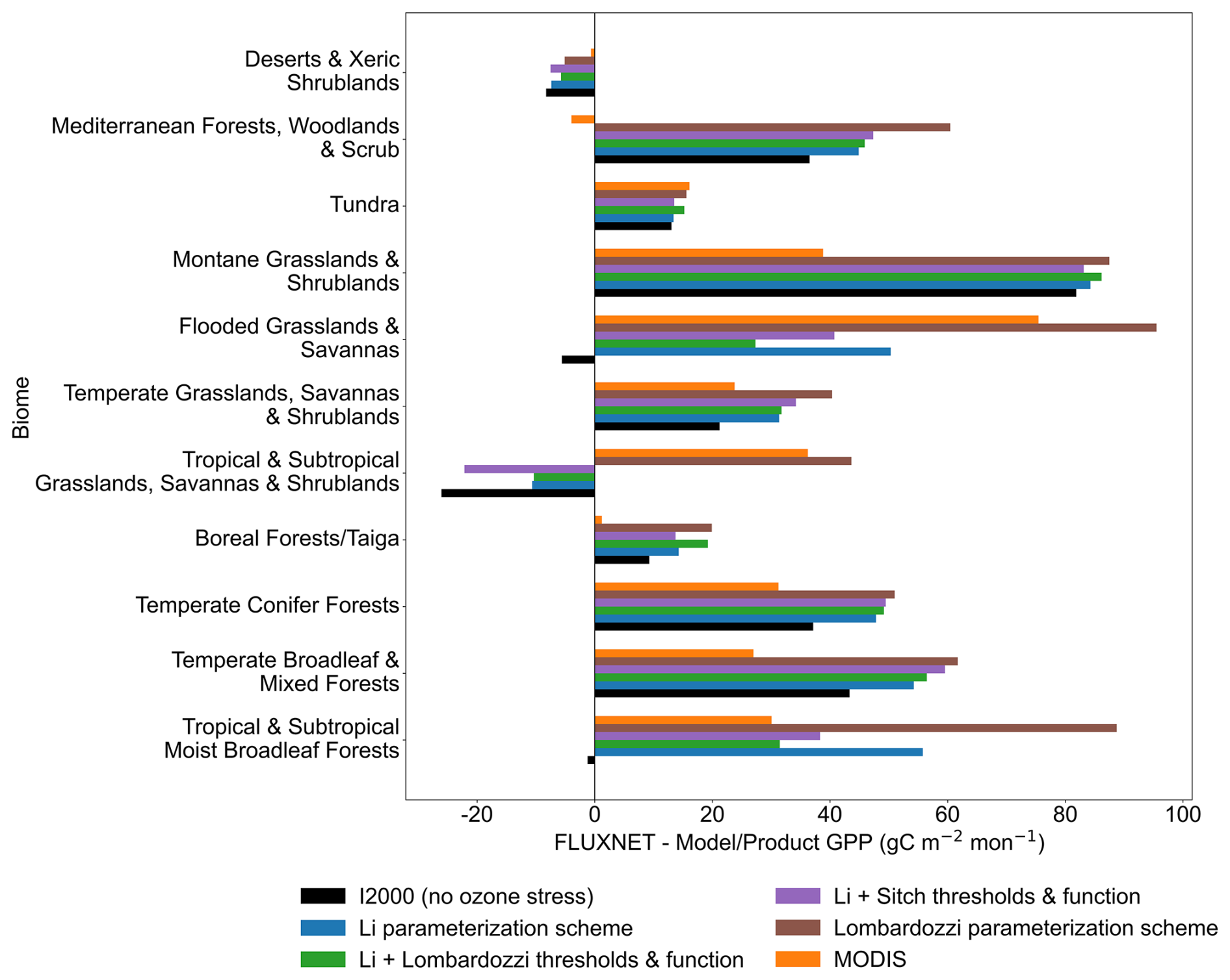
Table 3 Annual mean GPP bias relative to FLUXNET across different ozone parameterization schemes.

The monthly mean GPP bias aggregated over eleven biomes shows a pronounced dependence on biome type (Fig. 4). In flooded grasslands and savannas, montane grasslands and shrublands, tropical moist broadleaf forests, and some other biomes, the bias is positive and relatively large, indicating that most parameterization schemes underestimate GPP in these biomes (since model GPP < observed, bias = model − obs > 0). The positive bias of the Lombardozzi parameterization scheme is the most pronounced in several of these biomes. The no-ozone case generally exhibits smaller biases than ozone-stress parameterization schemes across several temperate and boreal biomes, suggesting that introducing ozone stress alone does not necessarily improve model performance and that additional physiological or environmental constraints may still be required to better reproduce observations. In contrast, the magnitude of the bias is smaller in tundra, temperate grasslands/savannas/shrublands, and boreal forests (taiga), and the Li parameterization scheme and its threshold/function variants (Li + Sitch and Li + Lombardozzi) are overall closer to zero bias. In deserts and xeric shrublands, the biases are near zero. In tropical and subtropical moist broadleaf forests, the no ozone case shows a slight negative bias (model > obs in that biome, indicating overestimation), which is reduced after ozone stress is introduced (the ozone schemes dampen the model's overestimation).

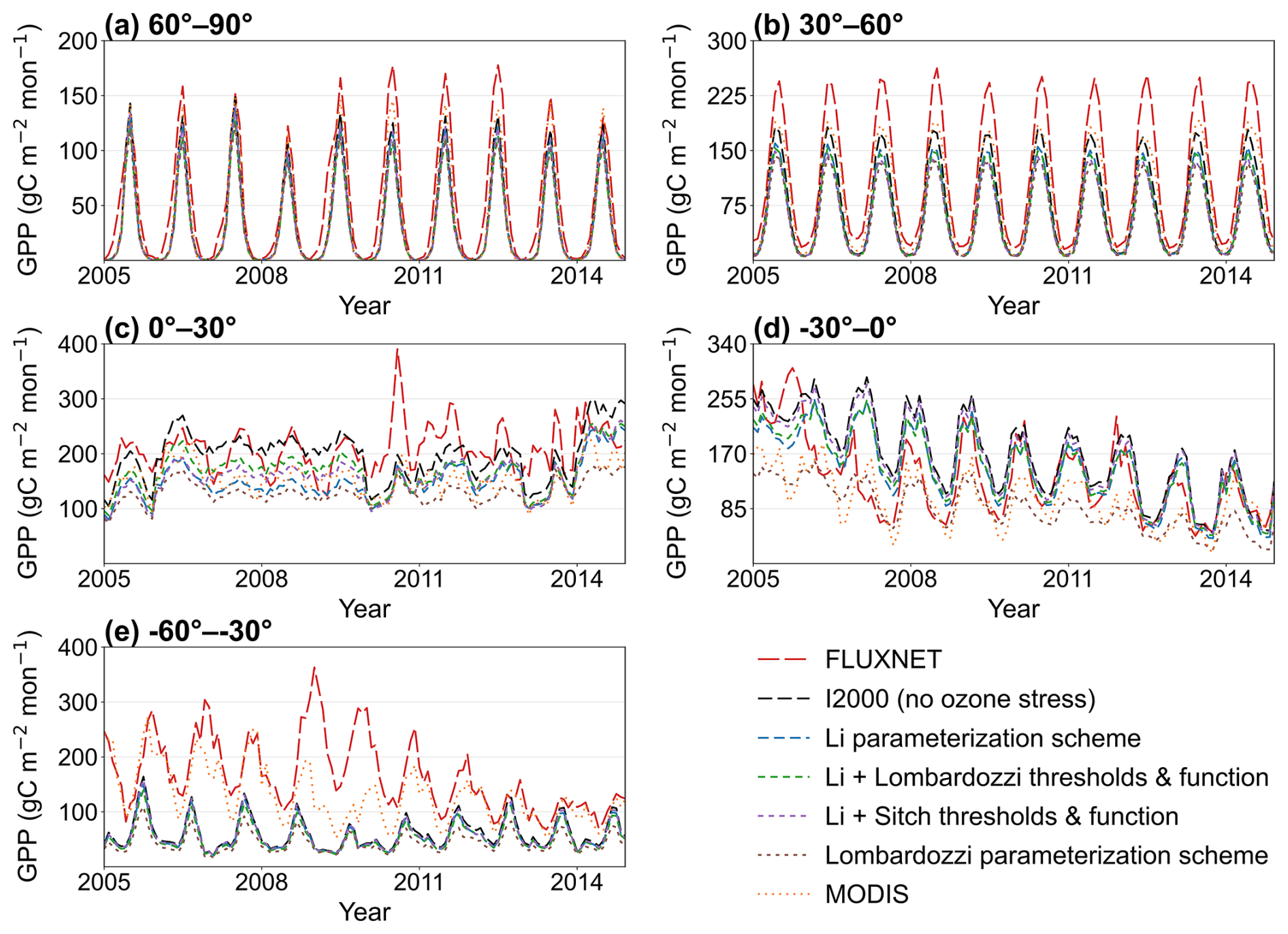
Figure 5 Monthly GPP time series for 2005–2014 in five latitude bands (60–90, 30–60N, 0–30° N, 0–30, and 30–60° S), comparing FLUXNET, the no-ozone experiment, ozone-stress parameterization schemes, and MODIS.

3.2 Temporal evaluation and verification of ozone stress parameterization schemes

The monthly GPP time series aggregated by latitude band show that the model generally reproduces the seasonal phase, but there are systematic differences in amplitude among the parameterization schemes (Fig. 5). At high northern latitudes (60–90° N), all schemes show peaks aligned with FLUXNET. MODIS, no ozone case, and the Li-family parameterization schemes (Li; Li with Lombardozzi thresholds/functions; Li with Sitch thresholds/functions) have amplitudes closest to the observations, while Lombardozzi shows a more pronounced underestimation of the summer peak. The no ozone case generally produces larger seasonal amplitudes than the ozone-stress parameterization schemes and, in several latitude bands, remains closer to FLUXNET during peak growing seasons, suggesting that introducing ozone stress alone cannot fully resolve the discrepancies between simulations and observations. In the midlatitudes of the Northern Hemisphere (30–60° N), all schemes systematically underestimate FLUXNET, and the degree of underestimation increases progressively from MODIS to the Li family of ozone stress schemes to Lombardozzi. This highlights differences arising from limitations in the model's intrinsic simulation skill and spatial resolution (a similar systematic underestimation is also found by Wild et al., 2022, for coarse-scale models). In the tropics and subtropics (0–30° N), seasonality is weaker and interannual variability is more pronounced. Except for the no-ozone case (which overestimates in some months), the other parameterization schemes all show some degree of underestimation, though the magnitude is smaller than in the northern midlatitudes. The low latitudes of the Southern Hemisphere (0–30° S) show a similar pattern, but the simulations agree better with the observations (the time-series curves overlap FLUXNET almost entirely for some schemes). At midlatitudes in the Southern Hemisphere (30–60° S), there is persistent underestimation during several growing seasons. It is noteworthy that, although these time series exhibit systematic biases, the results for the southern midlatitudes indicate that the Li parameterization scheme provides the best simulation (its curve is closest to the FLUXNET curve).

The monthly GPP time series aggregated by plant functional type (PFT) show that all parameterization schemes can generally reproduce the seasonal phase, but there are consistent and type-dependent systematic differences in amplitude (Fig. 6). For broadleaf trees and needleleaf trees (Fig. 6a and b), all five simulations and MODIS underestimate FLUXNET as a whole, with the underestimation of the growing season peak being most pronounced. In these forest PFTs, the no ozone case generally produces larger seasonal amplitudes and remains closer to FLUXNET during peak growing periods than most ozone-stress parameterization schemes. For shrubs (Fig. 6c), seasonality is weaker and interannual variability is larger; in the no-ozone case, schemes tend to overestimate, whereas the introduction of ozone stress leads to convergence among the schemes, most evident in the Li parameterization scheme (Li matches the observed shrub GPP level best). Grasslands and crops (Fig. 6d and e) show strong seasonal oscillations and are overall underestimated relative to the observations, but they generally perform better (closer to observations) than the broadleaf and needleleaf trees. As in Fig. 5, unavoidable systematic biases pose challenges for evaluation, but notably, the time series for shrubs again indicate that the Li parameterization scheme is optimal (it most effectively reduced the shrub GPP overestimation present in the no-ozone case).

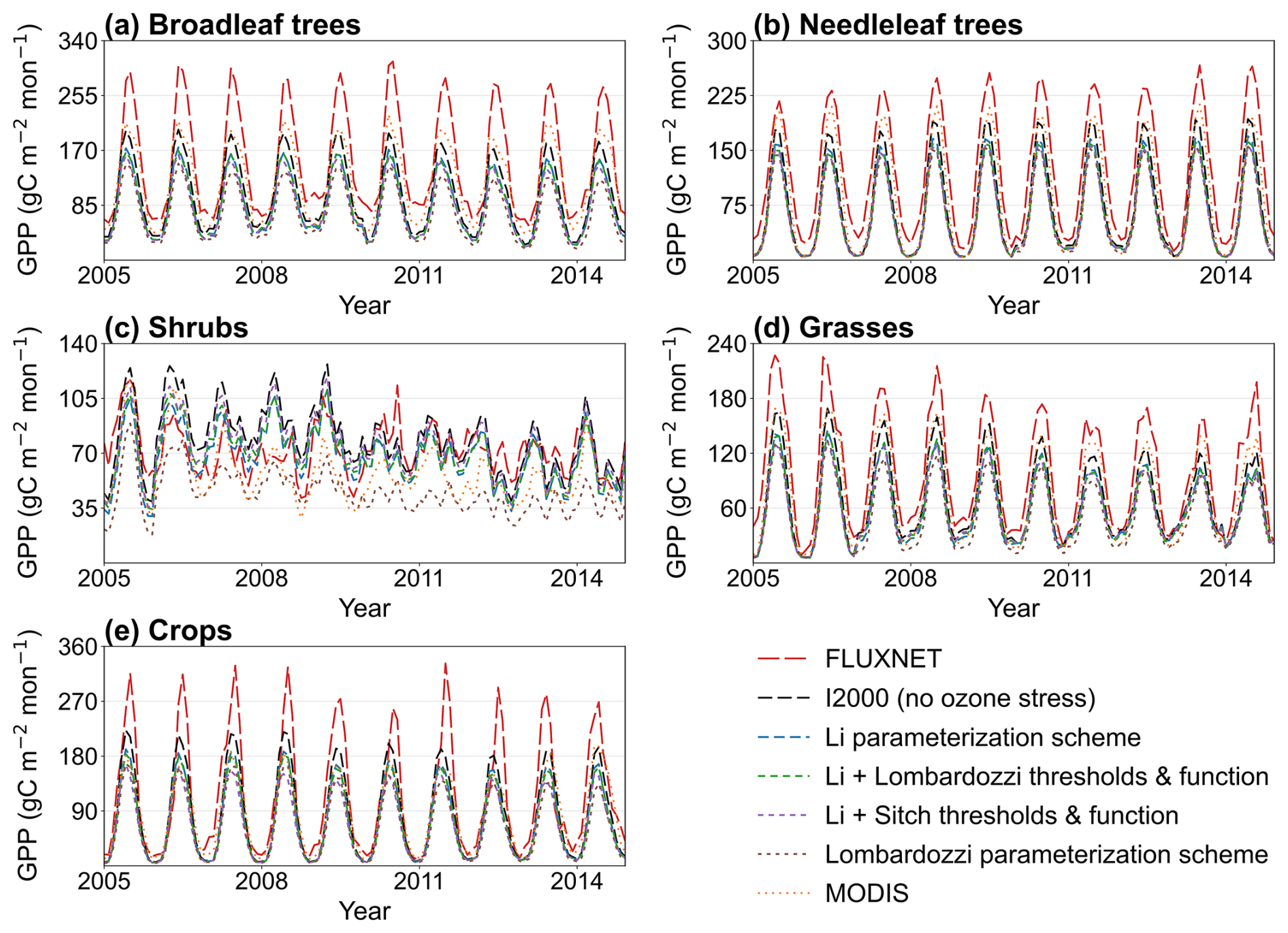
Figure 6 Monthly GPP time series for 2005–2014 by plant functional type (broadleaf trees, needleleaf trees, shrubs, grasses, and crops), comparing FLUXNET, the I2000 no-ozone experiment, ozone-stress parameterization schemes, and MODIS.

3.3 Overall evaluation and verification of ozone stress parameterization schemes

The seasonal reproduction of monthly GPP by each parameterization scheme and product is at a moderate level, with r mostly in the range from 0.4 to 0.6, and the normalized standard deviation at most sites being less than 1 (Fig. 7). This indicates that the model and MODIS both show varying degrees of variance damping relative to FLUXNET (both underestimate variability). Among the ozone parameterization schemes, the Li scheme has correlation and normalized standard deviation values closer to FLUXNET than those of the others. The no-ozone case and the Li parameterization scheme yield higher correlations for most vegetation types, and the Li scheme is closest to the observed amplitude for shrubs, consistent with Fig. 6, which shows that the Li scheme significantly reduced shrub biases. Compared with ozone-stress parameterization schemes, the no-ozone case generally exhibits higher normalized standard deviations across several PFTs, indicating stronger preservation of seasonal variability. However, its correlations are not consistently the highest, and its performance for shrubs and crops is poorer than that of some ozone-stress parameterization schemes. The Li + Sitch, Li + Lombardozzi, and Lombardozzi parameterization schemes exhibit varying degrees of discrepancy, and their correlations and normalized standard deviations are, overall, smaller (worse) than those of the Li scheme. MODIS shows both lower correlation and lower normalized standard deviation for most types (partly reflecting that MODIS GPP is a remote-sensing estimate with its own uncertainties).

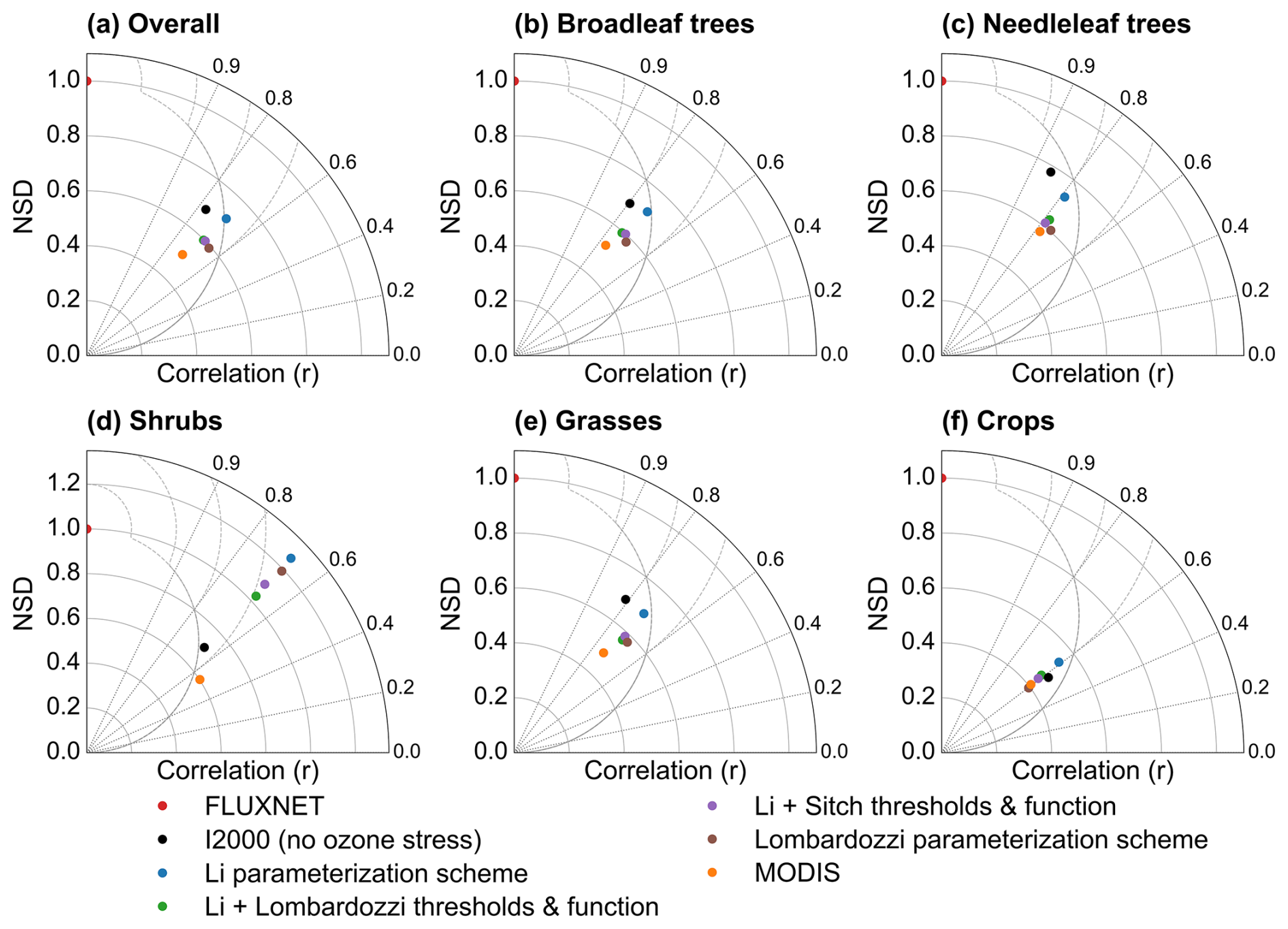
Figure 7 Correlation (r) and normalized standard deviation (NSD) of monthly GPP (2005–2014) relative to FLUXNET for all sites combined and for five plant functional types, comparing the I2000 no-ozone experiment, four ozone-stress parameterization schemes (Li, Li with Lombardozzi thresholds and function, Li with Sitch thresholds and function, and Lombardozzi), and MODIS.

Seasonal Nash–Sutcliffe efficiency (NSE) shows that MODIS consistently gives the highest agreement with FLUXNET, with excellent performance in winter and autumn (Fig. 8). Among the model experiments, the no ozone case generally maintains the highest NSE values in spring, summer, and autumn, indicating that the baseline simulation without ozone stress still reproduces seasonal variability better than most ozone-stress parameterization schemes at the large scale. For the ozone stress parameterization schemes, summer (JJA) is the weakest season for all schemes: no ozone case reaches only 0.10 and all schemes turn negative in NSE after ozone stress is introduced, indicating a deterioration in the fit to FLUXNET during peak growth months. In spring (MAM), the no-ozone case is NSE ≈ 0.26, while the ozone parameterization schemes range from 0.13 to 0.24 and are slightly lower overall. In autumn (SON), the no-ozone case is 0.21, while the ozone schemes range from 0.02 to 0.12 and remain lower. In winter (DJF), all model schemes perform well (NSE near 0.5–0.7), and the differences between the no-ozone case and the Li parameterization series are very small.

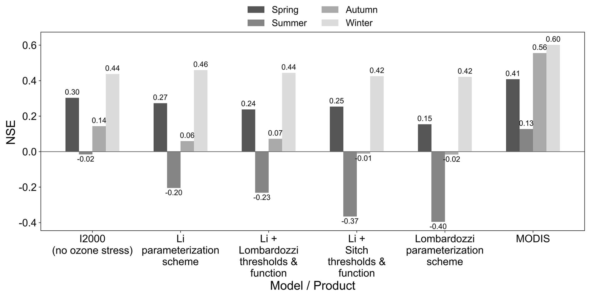
Figure 8 Seasonal Nash–Sutcliffe efficiency (NSE) of monthly GPP relative to FLUXNET (2005–2014) for the I2000 no-ozone experiment, four ozone-stress parameterization schemes (Li, Li with Lombardozzi thresholds and function, Li with Sitch thresholds and function, and Lombardozzi), and MODIS. Panels (a)–(d) correspond to spring (MAM), summer (JJA), autumn (SON), and winter (DJF), respectively.

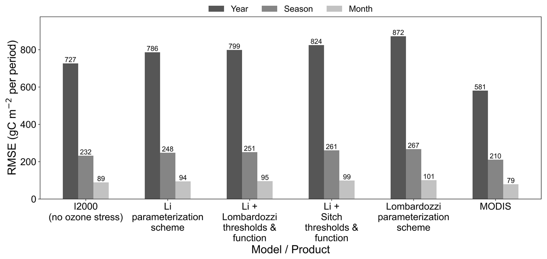
Figure 9 Root mean square error (RMSE) of GPP relative to FLUXNET (2005–2014), evaluated from monthly data at three temporal aggregation scales (annual, seasonal, and monthly) for the I2000 no-ozone experiment, four ozone-stress parameterization schemes (Li, Li with Lombardozzi thresholds and function, Li with Sitch thresholds and function, and Lombardozzi), and MODIS.

From the annual, seasonal, and monthly levels, RMSE increases markedly as the aggregation scale becomes finer (annual < seasonal < monthly), and importantly, the ranking of the parameterization schemes remains consistent across the different levels (Fig. 9). This consistency is similar to the interannual-scale RMSE results in the study of Wild et al. (2022). The no-ozone case consistently shows lower RMSE values than all ozone-stress parameterization schemes at the annual, seasonal, and monthly scales, suggesting that additional sources of model uncertainty beyond ozone stress may still contribute to discrepancies relative to FLUXNET. Among the model parameterization schemes, the Li scheme has the smallest error, followed by Li + Lombardozzi, Li + Sitch, and Lombardozzi; the Lombardozzi scheme has the largest error at each time-scale. MODIS yields the lowest RMSE at all three levels and is closest to FLUXNET among all model schemes. Overall, after ozone stress is introduced, the RMSE of the parameterization schemes does not decrease uniformly relative to the no-ozone experiment (in some cases, ozone stress introduces model bias, with persistent underestimation). Comparing the ozone stress parameterization schemes, the Li scheme shows the lowest RMSE at the annual, seasonal, and monthly levels.

The ten-year mean global total GPP shows that the no-ozone experiment produces a higher global total GPP, and that the inclusion of ozone stress reduces this total by about 10 % to 24 % across the schemes (Fig. 10). The no ozone case reaches 132.00 Pg C yr⁻¹, substantially exceeding both MODIS and FLUXCOM estimates, indicating that neglecting ozone stress likely leads to an overestimation of global terrestrial productivity. Among the four schemes, the Li family of parameterization schemes (Li, Li + Lombardozzi, Li + Sitch) is closer to MODIS (112.51 Pg C yr⁻¹). Additionally, the FLUXCOM upscaling estimate of ∼115.2 Pg C yr⁻¹ suggests that the Li parameterization scheme is closest to the observations, whereas the Lombardozzi result is clearly lower (Li et al., 2024). In other words, the more substantial ozone damage in the Lombardozzi scheme yields a larger global GPP reduction (∼24 %) than appears warranted by satellite-derived GPP benchmarks (∼10 %–12 % reduction), while the Li scheme's more moderate effect (∼12 % reduction) aligns better with observed totals.

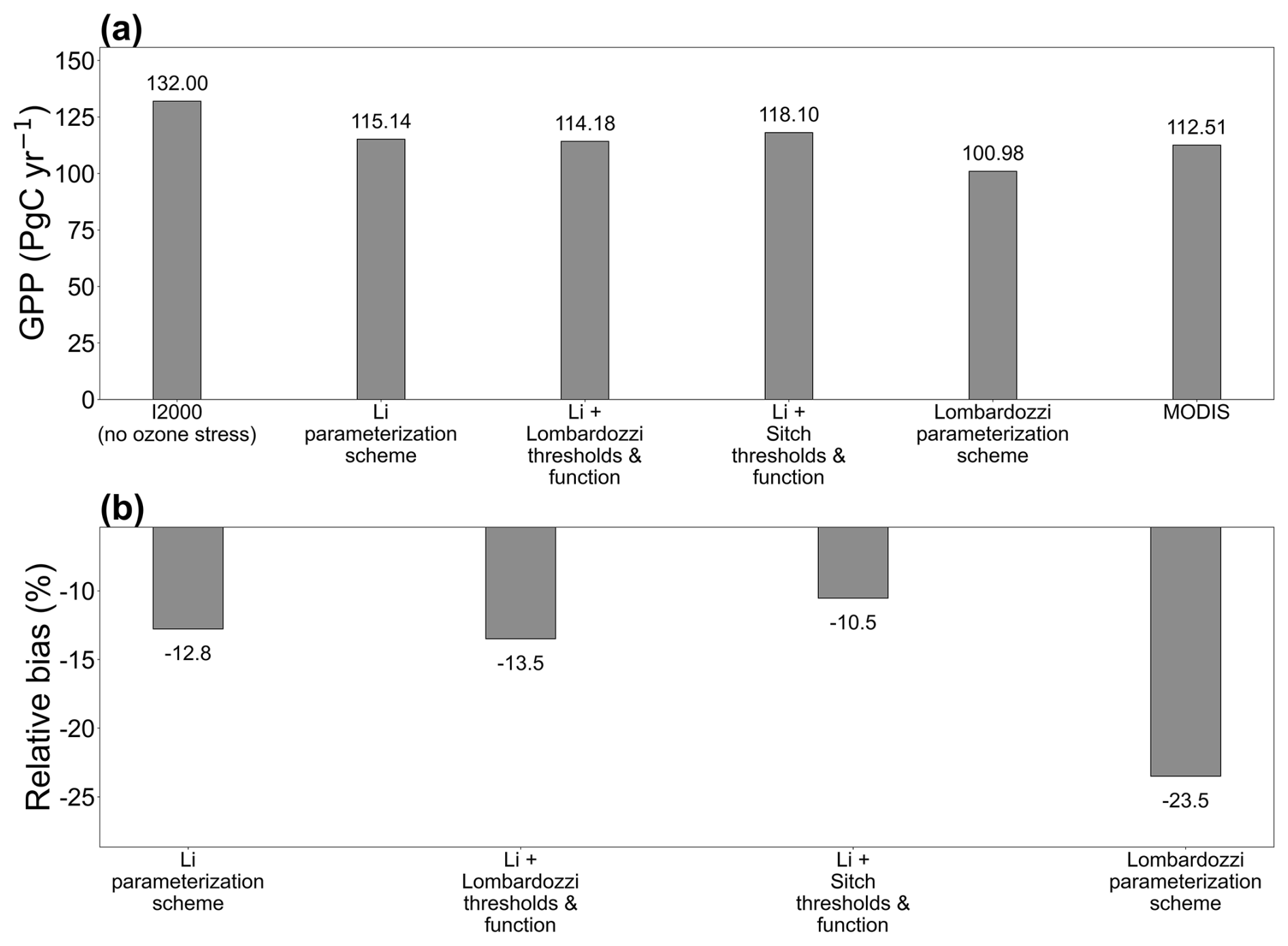
Figure 10 Decadal-mean (2005–2014) global total GPP and relative bias for four ozone-stress parameterization schemes and MODIS, compared with the I2000 no-ozone experiment. (a) Global total GPP; (b) relative bias (%).

4 Discussion

The spatial heterogeneity and zonal structure of ozone impacts on productivity can be understood as the coupled outcome of multiple processes. High radiation, together with relatively open stomata, increases stomatal flux, thereby more easily triggering above-threshold accumulation and physiological suppression (Mills et al., 2018). In contrast, under low-temperature, drought, or stomatal-closure conditions, effective flux and cumulative dose can be suppressed even when ozone concentration is relatively high (Liu et al., 2024). These features suggest that the priority for parameterization schemes should be explicit gating and adaptive thresholds for radiation and turbulent transport, evapotranspiration and stomatal limitation, and phenology and canopy stratification (Clifton et al., 2020). From a mechanistic perspective, the Li framework parameterization scheme uses data-driven ozone flux thresholds and separate responses of photosynthesis and conductance, thereby improving its ability to represent flux triggering under tropical conditions with high radiation and humidity (Li et al., 2024; Pande et al., 2025). By contrast, the Lombardozzi parameterization scheme, which uses cumulative uptake as a state variable, exhibits a strong memory effect and accumulates ozone damage too rapidly under sustained high-flux conditions. Together with a relatively rigid scaling relation, it tends to amplify long-term suppression at low latitudes, leading to systematic GPP underestimation (Visser et al., 2021). Consistent with this, a recent model comparison in China showed that the Lombardozzi scheme produced GPP losses 2.5–4 times larger than those of the Sitch scheme, reflecting an over-accumulation of ozone damage in regions of high exposure (Cao et al., 2024). In terms of model structure, a weakly coupled pathway that first accumulates flux above the threshold and then scales a solution without ozone can partly avoid excessive coupled amplification of evapotranspiration, conductance, and photosynthesis, thereby reducing systematic bias in the tropics (Otu-Larbi et al., 2020). The comparison results show that what is decisive is not only whether ozone is represented, but also how ozone flux thresholds and response functions are defined and how memory and radiation stratification are treated at the canopy scale (Zhou et al., 2024).

Station-based RMSE, together with biome-mean bias, jointly reveal a three-way constraint arising from observations, simulations, and spatial resolution. On the one hand, complex land surfaces and diverse PFT combinations in the midlatitudes produce bands of significant errors, while higher-resolution remote sensing in the same regions shows fewer extreme high values, indicating that grid-scale mismatch and subgrid heterogeneity are essential sources of information loss (Wild et al., 2022). On the other hand, under the same forcing, the Li series of parameterization schemes shows convergence in RMSE and reduced bias across several latitude bands and biomes, indicating that a strategy in which ozone flux thresholds can be optimized, and response functions selected, is more favorable for transfer across ecological zones. In contrast, the Lombardozzi parameterization scheme tends to accumulate more strongly and impose more profound suppression in low latitudes and in some grass and shrub systems. It therefore requires region-specific adjustments to ozone flux thresholds and response functions (e.g., separate calibration for sensitive tropical ecosystems). Integrated statistics across multiple biomes also show that the biases exhibit pronounced biome dependence, underscoring that a one-size-fits-all ozone parameterization will lead to systematic errors in specific biomes (e.g., savannas, montane shrublands).

Experimental evidence from previous ozone exposure studies also suggests that the ozone flux thresholds currently adopted across different parameterization schemes remain highly uncertain across vegetation types. For example, experiments comparing loblolly pine (needleleaf) and yellow-poplar (broadleaf) showed stronger ozone sensitivity in the needleleaf species (Tjoelker and Luxmoore, 1991), whereas studies on Magnolia denudata and Cotinus coggygria indicated that broadleaf trees could be more ozone-sensitive than shrub species (Xu et al., 2021). Other controlled experiments further suggested a sensitivity gradient of soybean > tobacco > poplar, implying that crop species are generally more sensitive to ozone than many broadleaf woody species (Dai et al., 2019). However, the Lombardozzi parameterization scheme applies a uniform threshold of 0.8 nmol m⁻² s⁻¹ to all five vegetation categories, which may oversimplify species- and PFT-dependent detoxification capacity. Similarly, the original Sitch scheme was developed under limited observational constraints, lacking dedicated experimental evidence for shrub and grass vegetation types; therefore, shrub thresholds were assumed to be equivalent to those for broadleaf vegetation, while grass thresholds were assumed to be similar to those for crops. In contrast, the Li scheme assigns higher ozone sensitivity to needleleaf forests than to broadleaf forests, a result that is not always consistent with the experimental evidence summarized above. Taken together, these inconsistencies indicate that ozone flux thresholds remain insufficiently constrained and still require further recalibration across vegetation types and model frameworks.

This uncertainty was one of the primary motivations for introducing the mixed parameterization experiments in this study. By combining the Li framework with alternative threshold and response-function settings from the Lombardozzi and Sitch schemes, we aimed to isolate the effects of threshold definitions and response-function forms from other structural components of the parameterizations. Importantly, we did not perform additional retuning or recalibration of the empirical parameters, including the global parameter originally used in the Sitch scheme, when transferring these thresholds and response functions into the Li framework. Therefore, the mixed experiments should be interpreted as structural-sensitivity experiments rather than as optimized implementations. In addition, comparing the Li+Lombardozzi and original Lombardozzi schemes enabled us to distinguish further the role of cumulative memory effects from that of threshold and response-function choices alone. Our results suggest that differences in long-term ozone accumulation and canopy memory can substantially alter the magnitude and spatial pattern of simulated ozone damage, even under similar threshold settings.

Except for a few regions, most parameterization schemes still show systematic underestimation to varying degrees across several seasons. Therefore, we focused on the prominent overestimation of the no-ozone experiment relative to the observations in the low latitudes of the Southern Hemisphere (approximately 30° S to the equator) and in shrub-dominated regions, where the time series matched better after introducing ozone (Figs. 5 and 6c). This latitude band is primarily a transition zone from subtropical to tropical semiarid and monsoon climates, where intense radiation and relatively open stomata, together with enhanced boundary-layer mixing during the rainy season, tend to increase instantaneous stomatal flux (Khan et al., 2025). If the gating of above-threshold accumulation or CUO is insensitive to high afternoon vapor pressure deficit (VPD) and soil moisture constraints, or if the phenological switches and leaf-age decay associated with transitions between wet and dry seasons are not adequately represented, potential productivity will be overly amplified (Eghdami et al., 2022). Shrub ecosystems often have shallow roots and rapidly renewing leaves, coexist with shrub–grass mosaics, and are subject to grazing disturbance; in reality, stomatal regulation is more conservative and strongly driven by soil moisture pulses (Wang et al., 2018). When a parameterization scheme adopts forest-type ozone flux thresholds or fixed-shape response functions and does not distinguish the time-varying weighting of canopy flux under heterogeneous near-surface turbulence and radiation, the model tends to produce amplified GPP peaks after rainfall events or at the beginning of the growing season, resulting in systematic overestimation relative to FLUXNET (Vermeuel et al., 2024). In contrast, the Li parameterization scheme uses data-driven thresholds and selectable, decoupled response functions for photosynthesis and conductance, and its treatment of canopy stratification and phenological gating is more consistent with process constraints. As a result, in the band from 30° S to the equator and in shrub-rich regions, the Li scheme markedly reduces the overestimation and comes closer to FLUXNET.

Compared with the earlier CLM4.5-based study by Lombardozzi et al. (2015), an important difference emerges in the baseline productivity simulated in the absence of ozone stress. In CLM4.5, the no-ozone global GPP reached approximately 146.5 Pg C yr⁻¹, whereas the corresponding no-ozone simulation in the present CLM5 framework is substantially lower (132 Pg C yr⁻¹). This indicates that improvements in the underlying land-surface physiology and canopy process representation from CLM4.5 to CLM5 have already reduced part of the excessive global productivity bias. Consequently, introducing ozone stress in CLM4.5 moved the simulated GPP closer to observational benchmarks at the global scale, whereas in CLM5, the remaining correction space is smaller, and excessive ozone suppression can more readily lead to underestimation in some regions and across statistical metrics. This difference highlights that the apparent performance of ozone-stress parameterizations is strongly dependent on the baseline behavior of the host land-surface model.

From the perspective of global total GPP, the reasons why different ozone stress parameterization schemes produce varying degrees of reduction lie mainly in how ozone flux thresholds are determined and in the forms of the response functions. A framework in which thresholds are determined from data and the optimal choice can be made among several candidate functions helps calibrate, separately, when ozone stress is triggered and how strongly it decays after triggering. This maintains transparency and traceability when applied across regions. In contrast, configurations with overly strong cumulative memory more easily amplify the influence of historical fluxes in low-latitude ecosystems with high leaf longevity or long growing seasons. Our results here support the findings of Li et al. (2024) on a global scale: using PFT-specific optimal thresholds and nonlinear response curves (as in Li's scheme) yields roughly half the ozone-induced GPP reduction compared with a scheme with fixed thresholds and linear responses, thereby better aligning model GPP estimates with observational estimates. Thus, beyond the inclusion of ozone damage per se, the calibration and flexibility of the threshold and response parameters determine model outcomes.

5 Implications for future improvement in Earth system models

The significant differences in GPP bias across biomes reveal key directions for improving ozone-stress parameterization in models. In biomes with intense radiation, such as wetland grasslands and tropical moist broadleaf forests, models generally underestimate GPP, especially with the Lombardozzi scheme. Therefore, regional calibration of ozone flux thresholds and response functions is needed for these areas. In contrast, in low-stress regions such as tundra, temperate grasslands, and forests, the Li scheme, with optimized thresholds and decoupled response functions, performs best, suggesting that more refined model adjustments are required in these regions. In dry and desert biomes, a slight overestimation is observed, especially in the no-ozone simulations, indicating that the model's performance is generally good in these regions but still leaves room for further improvement when accounting for other environmental factors. In conclusion, optimizing the model to account for the characteristics of different biomes will improve the accuracy of ozone-stress simulations, thereby enhancing the reliability of climate predictions. In addition, although the Li scheme performs well across most vegetation types, especially in shrubs, where it significantly reduces bias (as shown in Fig. 7), it does not always perform best in crop types and under autumn conditions. Particularly in summer, the NSE values for all ozone stress schemes are relatively low, and after ozone stress is introduced, the model's fit to FLUXNET deteriorates. This indicates that, although the Li scheme performs well in certain biomes and seasons, further optimization is still needed for crop types and seasonal variations.

The process representation of ozone stress effects needs to shift from a paradigm of static ozone flux thresholds combined with fixed response functions to parameterization schemes based on a unified mechanistic framework that can be transferred across different vegetation types and regions. We should calibrate ozone flux thresholds for different vegetation types and areas in a data-driven manner, enabling optimal selection among multiple response functions while accounting separately for the independent suppression of photosynthesis and stomatal conductance. In parallel, we recommend introducing finer control over canopy stratification, phenological gating, and leaf-age memory, so that above-threshold accumulation or dose state variables can adapt across diurnal, seasonal, and growth stages, thereby avoiding systematic excessive downregulation caused by long-term memory.

Interactions between ozone stress and water stress need to be incorporated in parallel rather than corrected afterward. Under conditions of high temperature, intense radiation, and elevated VPD, whether above-threshold accumulation is triggered and how strongly it decays after triggering depend on the combined constraints imposed by evaporative demand, stomatal opening, and soil moisture. We recommend explicitly coupling the time-varying effects of VPD and soil moisture on stomatal and boundary-layer fluxes in the resistance-chain calculations, and setting robust gating for extreme afternoon conditions to reduce the degradation of model skill in summer. At the same time, for semiarid and shrub ecosystems, thresholds and response functions should be recalibrated using regional observations to avoid systematic over- or underestimation arising from the reuse of forest-type parameterization schemes. (Consistent with these recommendations, recent studies have called for jointly accounting for drought and ozone – e.g., Otu-Larbi et al. (2020) and Khan et al. (2025) – to better simulate vegetation risk.)

In addition to improvements to ozone stress parameterization schemes that need to infer thresholds, response functions, and water stress effects from in situ ground observations, previous studies have also discussed potential directions for development in terms of other explanatory variables such as leaf area, leaf thickness, and leaf mass per area, as well as additional environmental factors (Karlsson et al., 2007; Wittig et al., 2007; Bussotti, 2008; Feng et al., 2018; Hansen et al., 2019; Xu et al., 2020; Ma et al., 2023; Li et al., 2024). Here, we propose several potential directions from a remote sensing perspective for further improving model simulation ability and ozone stress parameterization schemes:

1. Photosynthetic capacity and stress detection: solar-induced chlorophyll fluorescence and the near-infrared vegetation index can be used as joint constraints on photosynthetic potential and non-photochemical quenching (Porcar-Castell et al., 2014; Badgley et al., 2017). Meanwhile, microwave vegetation optical depth, together with passive microwave soil moisture, can be used to characterize canopy water content and soil moisture state. These could help ensure that stomatal opening/closure and the conditions under which above-threshold O₃ uptake occurs are more accurately constrained under high-temperature, high-radiation conditions (Konings et al., 2017).

2. Canopy structure and turbulence: multi-source leaf area index products and emerging canopy structure observations (e.g., from LiDAR) can be used to better constrain canopy layer weighting and vegetation structural representation (Xiao et al., 2019). Additionally, canopy height and surface roughness inferred from LiDAR and synthetic aperture radar can be used to reduce systematic bias under conditions of strong afternoon turbulence and intense radiation (Dubayah et al., 2020). This would refine how models partition ozone flux between tall, rough canopies and short, smooth ones, thereby improving the partitioning of flux to leaves (Visser et al., 2021).

3. Plant traits and species-specific responses: leaf economic spectrum traits retrieved from hyperspectral observations – such as leaf mass per area (LMA), leaf thickness, and leaf nitrogen content – can be used to construct prior distributions of photosynthesis and conductance sensitivity for different vegetation types. This can support the dynamic, regional and seasonal updating of ozone flux thresholds and response functions (Serbin et al., 2014). For example, trait-based approaches (e.g., Ma et al., 2023) can inform which ecosystems have inherently higher ozone tolerance and should have higher threshold Y values in models.

4. Data assimilation and uncertainty quantification: through joint assimilation of site observations and remote sensing data, ozone flux thresholds, response function shapes, and key trait parameters can be calibrated and their uncertainties quantified simultaneously using hierarchical Bayesian methods or surrogate models (MacBean et al., 2016). This would achieve consistent multi-scale constraints and provide a transferable evaluation framework spanning the site, regional, and global scales.

Additionally, artificial intelligence (AI) offers a potential technical pathway for further developing ozone stress parameterizations. On the one hand, AI-based surrogate models can approximate complex ozone flux calculations and nonlinear response processes while maintaining physical constraints, holding promise for reducing computational costs and thereby supporting the exploration of multi-parameter combinations (Lu and Ricciuto, 2019; Zhu et al., 2022). On the other hand, integrating site observations, remote sensing products, and model outputs into supervised or semi-supervised learning frameworks may help identify ozone flux thresholds, response function forms, and their dependencies on moisture, radiation, and phenological conditions from multi-source data, providing data-driven prior information for different vegetation types and regions (Sung et al., 2025). Furthermore, combining artificial intelligence with model–data assimilation may offer new pathways for jointly inverting ozone flux thresholds, response function parameters, and key leaf traits (Raoult et al., 2025). By integrating artificial intelligence with physical constraints, ecological mechanisms, and multi-scale observations, it is possible to develop more flexible ozone-stress parameterization frameworks that provide more robust support for global carbon cycle assessments and scenario projections.

6 Conclusion

Within a unified land surface model framework, we compared three representative ozone stress parameterization schemes and, by decomposing in layers the choices of ozone flux thresholds, the representation of cumulative dose, and the shapes of response functions, clarified that beyond whether ozone is included, the more critical question is how thresholds and responses are represented. The overall evidence shows that a diagnostic scheme that uses data-driven thresholds, models photosynthesis and stomatal conductance separately, and allows an optimal choice among multiple response functions is more favorable for transferable applications across regions, vegetation types, and time scales. In contrast, configurations with overly strong cumulative memory or rigid assumptions about thresholds and functions are more likely to amplify systematic biases in specific climate zones or habitat types. Based on the comprehensive evaluation, we conclude that the Li ozone stress parameterization scheme is the most robust and the most consistent with the observations in this study. Notably, the mixed experiments incorporating thresholds and response functions derived from the Sitch and Lombardozzi schemes were conducted without additional recalibration; therefore, the differences reported here primarily reflect structural sensitivities rather than fully optimized implementations of those parameterizations within the Li framework.

Large-scale remote sensing productivity benchmarks and high-resolution site-level flux observations are complementary in space, time, and process representation. This enables us to separate uncertainties in ozone thresholds and response functions from biases in forcing fields and observations. At the same time, the temporally and spatially consistent ozone forcing from the chemical transport model ensures mechanistic coherence between atmospheric inputs and land-surface processes. The resulting chain of evidence not only supports a quantitative discrimination of the relative performance of different ozone stress parameterization schemes but also points to directions for improvement. Namely, our results indicate that ozone flux thresholds need to be explicitly calibrated in both the regional dimension and the vegetation-type dimension; that response functions should remain flexible with respect to the nonlinear joint effects of high summer temperature, intense radiation, high VPD, and water constraints; and that canopy stratification together with phenological gating are key mechanisms for suppressing long-term over-memory and biases under extreme afternoon conditions. At a practical level, these findings help identify a prioritized set of ozone-related parameters and processes that warrant focused constraint in future model evaluation and model–data integration efforts.

Our results further suggest that the apparent benefit of introducing ozone stress depends strongly on the host land-surface model's baseline behavior. Compared with earlier CLM4.5-based studies, the no-ozone simulation in CLM5 already produces substantially lower global GPP, indicating that improvements in canopy physiology and land-surface process representation have reduced part of the intrinsic productivity bias. Consequently, although ozone stress effectively reduces the tropical overestimation observed in the no-ozone experiment, improvements in model performance remain spatially and temporally heterogeneous across evaluation metrics and ecosystems. This highlights that future ozone parameterizations should not only focus on representing ozone damage itself, but also on achieving balanced interactions with the underlying model structure, including canopy processes, phenology, hydrological constraints, and biome-dependent productivity dynamics.

We also highlight limitations and frontier needs that still require attention. First, representativeness differences between the site scale and the model grid scale, together with subgrid heterogeneity, continue to amplify biases in some biomes and climate zones. This calls for higher-resolution forcing and parameter fields, as well as joint assimilation of site observations and remote sensing data, to narrow this gap. Second, the parallel systems for water and ozone stress still need strengthening. Future work should explicitly couple, at the level of the resistance chain, the time-varying modulation of stomatal flux and boundary-layer flux by vapor pressure deficit and soil moisture, and should use hierarchical Bayesian or surrogate-model approaches to calibrate the thresholds, response functions, and prior distributions of key leaf traits in ozone stress parameterization schemes. Third, regional calibration of thresholds and ecosystem-type-specific response functions still requires richer observational evidence, especially in semiarid shrublands, tropical monsoon regions, and cropland systems under strong management. Strengthening these aspects is expected to extend the diagnostic framework for ozone flux threshold calibration and response function selection developed in this study into a consistency evaluation tool applicable across multiple scenarios and models, thereby enhancing the transferability and credibility of assessments of ozone impacts on the carbon cycle.