Optimisation of ICON-CLM for the EURO-CORDEX domain: developments, sensitivities, tuning

Optimising the model performance to reduce model biases is a challenging task in global and regional climate modelling, especially relevant for free-running climate change simulations. This challenge is addressed in the present study through a systematic regional climate model tuning strategy using a novel methodology, which includes an iterative update of the reference configuration and combines expert judgement with objective tuning using a Linear Meta-Model optimisation (LiMMo) to derive an optimised model configuration. We applied this methodology to the regional climate model ICON-CLM setup over Europe at 12 km grid size (EURO-CORDEX domain) in order to reduce, e.g., the overestimation of incoming solar radiation and too low 2 m temperature. During this process, the sensitivity of the model to changes of 29 model parameters and their physical consistency was tested and investigated. Comparing the results of optimisation by expert judgement with those of LiMMo showed that the latter not only confirmed the expert judgement by focusing on a priori known highly sensitive parameters, but also allowed for fine-tuning of the model configuration with explicit control over the tuning process, making parameter combinations more efficient. With reference to the default ICON numerical weather prediction configuration, the model optimisation yielded significant improvements for a real climate mode simulations use case. For example, biases in incoming short wave radiation could be reduced by 30 %, latent heat flux biases by 15 %, by tuning cloud parameters in combination with surface flux parameters. Furthermore, the new optimised configuration could only be reached by using updated, higher-quality external datasets, including transient aerosols. Based on the community-based coordinated parameter tuning, we recommend an ICON-CLM model configuration for the EURO-CORDEX domain that is already being used for the downscaling of global CMIP6 simulations.

1 Introduction

The Icosahedral Non-hydrostatic (ICON) model is a flexible and scalable high-performance modelling framework for weather, climate, and environmental predictions and projections (Zängl et al., 2015, 2022; Müller et al., 2025). ICON is a joint project of Deutscher Wetterdienst (DWD), Max-Planck-Institute for Meteorology (MPI-M), the German Climate Computing Center (DKRZ), the Karlsruhe Institute of Technology (KIT), and the Center for Climate Systems Modeling (C2SM). The Consortium for Small-Scale Modeling (COSMO, https://www.cosmo-model.org/, last access: 3 April 2026) and the Climate Limited-area Modelling Community (CLM-Community, https://www.clm-community.eu/, last access: 3 April 2026) are collaborating partners in the areas of limited-area numerical weather prediction (NWP) and regional climate modelling (RCM).

ICON was introduced for operational global weather predictions at DWD in 2015 and has developed into one of the world's leading weather prediction models in recent years, according to weather prediction skill scores. Due to the different time scales involved, the model quality requirements and verification/evaluation processes are different between NWP and RCM applications. The former is used for short-term weather forecasts (up to two weeks), while the latter is employed for long-term, free-running climate projections until the end of the 21st century or beyond. To use ICON for regional climate projections, however, some modifications to the model source code and adjustments of the model configuration and parameter settings are required.

To use ICON in climate limited-area mode (ICON-CLM), developments and adjustments began in September 2014 with the establishment of the CLM-Community ICON Project Group. Based on ICON release 2.6.1, the first version of ICON-CLM was presented in 2021 (Pham et al., 2021). This included the testing of domain decomposition, restarts, and usage of different time steps, with a horizontal resolution of R2B8 (approximately 10 km) over the limited area pan-European EURO-CORDEX domain. Although the initial evaluation of the first version of ICON-CLM showed very promising results, the model configuration was based on the default NWP configuration for global NWP simulations (Pham et al., 2021).

Since the last two years, new ICON versions have been released biannually. The ICON-CLM model has been used in various studies as both an atmospheric-only model (Sieck et al., 2026) and a regional Earth system coupled model (Ho-Hagemann et al., 2024; Maurer et al., 2026). It has been, or is currently being, used in several national projects to assess recent and future climate developments in Germany and Europe. These projects include NUKLEUS (Sieck, 2020), UDAG (Früh, 2023), DAS-Basisdienst (DWD, 2023) and CoastalFutures (Schrum, 2021). In these studies, different versions of ICON with various namelist or parameter settings were used. While the simulations generally agree well with observations, there is still potential to reduce model biases, particularly in radiation and cloud processes (Maurer et al., 2026). Up to now, no comprehensive tuning procedure has been used to optimise the model quality for ICON in RCM use. It is important to note that different ICON-CLM configurations (model version, forcing, domain, grid resolution) require their own tunings to achieve the best regional climate simulation for a specific research domain. This process requires a significant amount of effort from various members of the CLM-Community at different institutions.

Parameter tuning is essential in Earth system modelling to align simulations with observations, supporting applications from weather forecasting (Zängl, 2023) to climate projections (Mauritsen and Roeckner, 2020). An increase in model complexity and resolution increases computational demands, creating a need for efficient and transparent tuning methods. All methods rely on high-quality observational datasets, and the selection of these datasets can influence the results. Four main approaches are usually used in climate modelling (Hourdin et al., 2017). First, expert tuning based on a manual model configuration adjustment based on expert judgement and experience (e.g., Mauritsen et al., 2012). Second, metamodel-based tuning, where surrogate models approximate full simulations (Neelin et al., 2010; Bellprat et al., 2012). Third, Bayesian calibration, using uncertainty and prior knowledge to estimate model parameters (e.g., Hourdin et al., 2023). Fourth, hierarchical emulators, which combine multi-resolution outputs to balance cost and accuracy of simulations vs biases (e.g., Williamson et al., 2012).

One objective of the CLM-Community is to provide community members with well-tested and thoroughly evaluated model versions and setups. This is of particular importance for versions and configurations that will be used in production, e.g., in 2025 as part of the COordinated Regional Climate Downscaling Experiment (CORDEX, 2025) of the World Climate Research Programme (WCRP), as these data are frequently used for climate services, adaptation planning, and policy consultancy. An extensive evaluation of COSMO 5.0, the predecessor of ICON, was carried out by the CLM-Community in 2014/15 (Anders et al., 2024) and of COSMO 6.0 in 2023/24 (Geyer, 2026). These tests were organised into phases of internal community projects called COPAT (Coordinated Parameter Testing): COPAT1 for COSMO 5.0 and COPAT2 for COSMO 6.0. This procedure has now been repeated and advanced for ICON-CLM to release the first officially recommended version and configuration of ICON-CLM, which will be used to downscale global simulations of the Coupled Model Intercomparison Project Phase 6 (CMIP6;  Eyring et al., 2016) in the context of the European branch of the Coordinated Regional Downscaling experiment (EURO-CORDEX) of the WCRP. Therefore, the focus of this study is on the European domain, as many CLM Community member institutions primarily concentrate their research interests on Europe and run simulations for this region. The COPAT comprehensive tuning and evaluation activities are a highlight of the CLM-Community. To our knowledge, these activities have not been performed and reported in other regional climate model development communities, making the CLM-Community unique in this regard.

This paper has the following goals: (I) It provides a description of the complete RCM tuning strategy to optimise the configuration of ICON-CLM for the EURO-CORDEX domain with a resolution of 0.11° (approx. 12 km, Fig. S1 in the Supplement) for a real use case. (II) Additionally, it introduces necessary model developments and adjustments to improve performance. (III) To optimise the model quality, we started with extensive ICON-CLM sensitivity tests, which provide insights into general model behaviour. (IV) The ensuing expert tuning in combination with the novel Linear Meta Model optimisation tuning (LiMMo; Petrov et al., 2025) is demonstrated. LiMMo belongs to the second category of parameter tuning methods – the objective calibration. (V) Finally, an optimum ICON-CLM regional climate simulation configuration is derived and presented. Model simulations were objectively evaluated by comparing them with various observational and ERA5 reanalysis data (Hersbach et al., 2020). The tests were mainly conducted in 2023 and 2024, incorporating the ICON release 2.6.6 and the ICON open-source release icon_2024.07 (ICON partnership (DWD, MPI-M, DKRZ, KIT, C2SM), 2024). The final test was performed using version icon_2024.07, which incorporates all additional developments; hence, the optimised configuration is widely usable.

The paper is structured as follows. Section 2 presents the data and methods used in this study, including the RCM tuning concept and a detailed description of the procedures. Section 3 shows the results of the sensitivity study, tuning outcomes for ICON-CLM and a comparison of expert and objective LiMMo tuning. The last section concludes with a summary of findings.

2 Methods

We first introduce an overview of our four-stage RCM configuration optimisation procedure (Sect. 2.1) applied in this study (reference, measures, expert, and LiMMo tuning) and highlight the most relevant technical steps of the ICON-CLM configuration optimisation for each of the tuning methods. In Sect. 2.2, we outline ICON-CLM standard parametrisations and new developments considered in the optimisation procedure. In Sect. 2.3, we describe the basic model setup with special emphasis on the external datasets and the design of our study. Note that each configuration tested in the COPAT2 experiment has been assigned a unique identifier. In Sect. 2.4, we briefly describe the LiMMo tuning framework, i.e. the linear meta-model and the optimisation framework. This optimisation framework has been developed as part of the study presented in this paper and is described in detail by Petrov et al. (2025). In Sect. 2.5, we introduce the observational reference data and the evaluated model variables used in this study. Finally, we present the evaluation measures (Sect. 2.6).

2.1 Tuning Strategy

The tuning strategy has been developed during the COPAT2 initiative of the CLM-Community. It is designed to systematically tune RCMs. The strategy with its four stages is shown in Fig. 1 and briefly described below. It should be noted that stage 3 (expert tuning) and stage 4 (LiMMo tuning) are alternative methods of finding an optimised configuration. In our study, both methods have been applied.

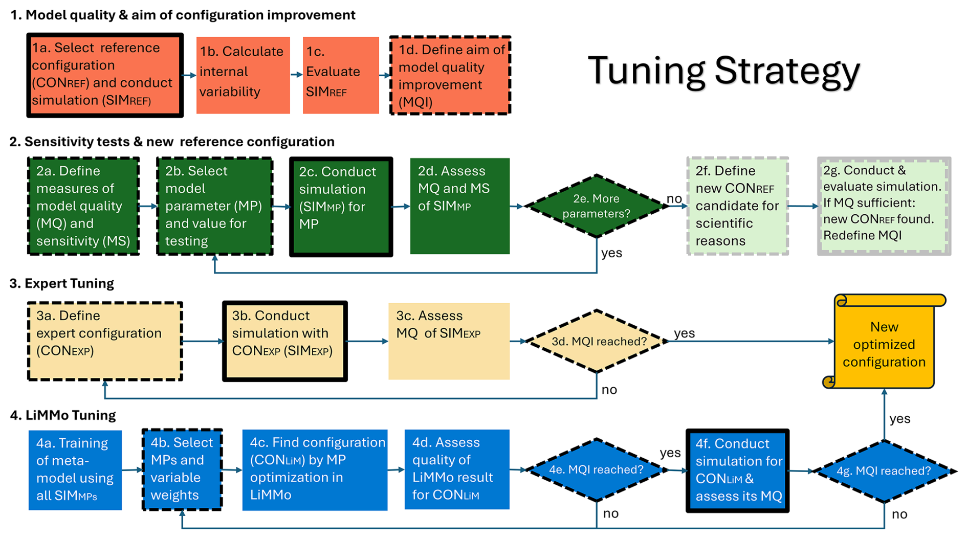
Figure 1 RCM tuning strategy framework. The four rows correspond to four stages. Rectangles correspond to activities, diamond-shaped polygons correspond to decisions. A thick solid frame (1a, 2c, 3b, and 4f) marks computationally intensive activities; a dashed frame (1d, 2a, 2b, 2e, 2f, 2g, 3a, 3d, 4b, 4e, and 4g) marks activities that require expert judgement. Light yellow and green colours indicate optional steps.

“The model quality & aim of configuration improvement” (row 1). A definition of the tuning aim (1d) is the starting point for the tuning process (rows 3 and 4). This requires selecting the initial configuration and performing the corresponding simulation (1a). The initial configuration might come from previous tuning initiatives or from other applications of the model (for example, from NWP configurations of a weather service). In this study, we used the configuration C2I101 suggested by the NUKLEUS project (see Sect. 2.3.2) as our initial configuration. The computation of the simulations' corresponding intrinsic variability came next (1b); it was determined by the monthly Root Mean Square (RMS) differences between two simulations with disturbed initial conditions (see Sect. 2.4.2 and Table 4). In this study perturbed simulations are identified as C2I200 and C2I207 (Table D1). Intrinsic variability is used to identify significant model biases and changes in RCM results due to configuration changes. It is also used to define the non-dimensional norm of a simulation's quality (see Sect. 2.4.2). Following that, the evaluation of the reference simulation (1c) takes place. The tuning aim (1d) depends on the evaluation in 1c and the general simulation purpose or aim, i.e., the intended use of the simulation. As the insight into model behaviour, sensitivity, and biases grows during the optimisation process, the tuning aim may be iteratively revised.

The second stage, “Sensitivity tests & new reference configuration” (row 2), consists of investigating the effects of single parameter changes and finding a new reference configuration that is better from a physical point of view than the initial one. The first step (2a) is devoted to the definition of the quality norm that quantitatively represents the tuning aim (1d). In our case, we use the comprehensive ScoPi score (see Sect. 2.6.1), the simple RMSE, and seasonal 2D biases to judge the quality of individual simulations compared to independent reference data. In addition, the sensitivity of the model with respect to parameter changes in its configuration is derived from parameter sensitivity tests (2a). To do so, we use the sensitivity measure presented in Sect. 2.6.2. The selection of the specific parameters of the configuration and their values to be tested (2b) is based on expert suggestions and the availability of newly developed external datasets that are relevant for climate simulations, like soil data, aerosols, orography, etc., which also affect the performance of a simulation (see Table 5). Once the simulations with the changed configurations and external parameters are conducted (2c), they are evaluated in terms of quality and sensitivity (2d). To efficiently analyse the model quality and model sensitivity, parameters are grouped according to physical processes in the model (Sect. 3.2). In our study, new reference configurations, C2I200c and later on C2I250c (Table C1), were found as a result of stage 2. Further results of stage 2 can be found in Sect. 3.2.

After conducting and evaluating all sensitivity tests for changes of single parameters in the model configuration in stage 2, the tuning effects of combined parameter changes are quantified. In the current study, we present two options for tuning: The first option, “Expert Tuning” (row 3), involves manual selection of parameter combinations based on insights from the previous stage, with the goal of reducing key model biases. The results are discussed in Sect. 3.4.1. The second option is the novel meta-model-based “LiMMo Tuning” (row 4), in which the user-defined optimisation procedure automatically selects parameter values. It is introduced in Sect. 2.4, and the results of its application are discussed in Sect. 3.4.2. An important advantage of LiMMo over expert tuning is that simulations with combined parameter changes are not needed for LiMMo tuning (compare 3b to 4f). Instead, users can use the meta-model like an experimental environment and obtain approximations of optimised configuration model results without performing computationally intensive simulations. In our study, as a result of expert tuning, the C2I268c configuration was found. The LiMMo optimisation yielded the C2I291c and C2I294c configurations (see Table C1).

2.2 ICON-CLM parameterisations

ICON-CLM is based on the limited-area mode of ICON for NWP. The core element of ICON-CLM is a non-hydrostatic, fully compressible numerical solver that is formulated on an icosahedral-triangular Arakawa-C grid and provides exact local mass conservation and mass-consistent tracer transport. In order to make ICON-CLM applicable in RCM applications, further developments and adjustments, such as transient anthropogenic greenhouse concentrations and aerosols or time-dependent sea surface temperatures, are included.

A detailed description of ICON dynamics can be found in Zängl et al. (2015) and first insights into the specialities of the climate mode in Pham et al. (2021). Here, we describe the relevant applied general physical parameterisations of ICON (Sect. 2.2.1). Afterwards, we discuss newly introduced climate-specific parameterisations of surface fluxes (Sect. 2.2.2) and cloud cover (Sect. 2.2.3) that turned out to be relevant in the course of the stage 2 model quality checking, which are meanwhile parts of the official ICON releases.

2.2.1 Standard physical parameterisations

“Fast physics” (called every advection time step): The land surface scheme TERRA (Schrodin and Heise, 2001; Schulz et al., 2016) provides vertical profiles of prognostic soil temperature, water, and ice for up to nine surface tiles (up to three different land use tiles, three snow tiles, and three water tiles). Recent developments include a new resistance-based formulation of bare soil evaporation and a new technique for computing the surface temperature, the so-called skin temperature (Schulz and Vogel, 2020). Both developments improve the prediction of the 2 m temperature, for instance, and other surface variables (Geyer, 2026). The effects of urban structures at the land surface are described by the urban model TERRA_URB (Wouters et al., 2016, 2017), which was ported from the COSMO model to ICON in the framework of the COSMO Consortium's Priority Project CITTÀ (Schulz et al., 2022; Campanale et al., 2025). The freshwater lake model FLake (Mironov, 2008) and a sea ice scheme derived from FLake (Mironov et al., 2012) provide prognostic surface temperatures over lakes and sea ice, respectively. The turbulent transfer and diffusion schemes of ICON are based on the Mellor-Yamada level-2 scheme, using a prognostic equation for turbulent kinetic energy (Raschendorfer, 2001). The turbulent transfer, i.e., the computation of transfer coefficients and with that of surface turbulent heat fluxes, is done on every surface tile. The grid-scale precipitation scheme accounts for precipitation formation over the ice phase, using the hydrometeor categories of cloud water, cloud ice, rainwater, and snow (Seifert, 2008).

“Slow physics” (called at lower frequency): The shortwave and longwave radiation are computed with “ecRad”, the radiation scheme of the European Centre for Medium-Range Weather Forecasts (ECMWF), as introduced by Hogan and Bozzo (2018). Its implementation in ICON is described by Rieger (2019). The Tiedtke-Bechtold scheme for shallow and deep convection (Tiedtke, 1989; Bechtold et al., 2008) was adopted from ECMWF's Integrated Forecasting System (IFS) model. The grid-scale effects by the sub-grid scale orography (SSO) are described by IFS's SSO scheme (Lott and Miller, 1997; Schulz, 2008), and grid-scale effects by the non-orographic gravity-wave drag are based on Orr et al. (2010). Cloud cover is represented by a diagnostic scheme using a quadratic distribution function of total water (sum of water vapour and cloud water) for liquid clouds, and an analogous equation for ice clouds, also taking convective anvils into account.

2.2.2 New developments in parameterisation of surface fluxes

The distribution of the incoming short-wave radiation between the components of the surface energy budget can be tuned by specifying scaling parameters. The sensitivities of the modelled climate with respect to the most important of these parameters have been tested during parameter optimisation in this study, however, near surface temperature biases remained and therefore, additional tuning parameters were introduced: the soil-moisture dependent tuning of the surface albedo and a factor on the minimum stomata resistance attributed to each land-use type given by external data (GLOBCOVER). These new parameters are part of the official ICON release now.

The portion of incoming solar energy absorbed at the surface depends on the surface albedo. Therefore, the albedo strongly influences the heating of the soil. In ICON-CLM, we prescribe monthly MODIS surface albedo (Schaaf and Wang, 2021) at the land surface. This encompasses the vegetation type and the bare soil albedo. A new parameter tune_albedo_wso (with its values abbreviated to taw) was introduced, correcting the albedo for very dry soils with taw1 and very wet ones with taw2 for the soil types sand, sandy loam, loam, and loamy clay (soil types 3–6 in TERRA). The idea behind this tuning is that wetter soils are darker and, thus, less reflective. The albedo α is corrected by α_c, dependent on soil moisture in the top soil layer $w_{\mathrm{so}}^{\mathrm{top}}$, whose thickness $\mathrm{\Delta }{z}_{\mathrm{so}}^{\mathrm{top}}$ is set to 10 mm in the parameterisation. The albedo for the near-infrared (nir), visible (vis), and ultraviolet (uv) wavelength bands α_i,0 is corrected as follows:

$$\begin{array}{}\text{(1)}& {\mathit{\alpha }}_i\left(w_{\mathrm{so}}^{\mathrm{top}}\right)=max[{\mathit{\alpha }}_{i,\mathrm{0}}\cdot (\mathrm{1}+{\mathit{\alpha }}_{\mathrm{vis},\mathrm{c}}\left(w_{\mathrm{so}}^{\mathrm{top}}\right)/{\mathit{\alpha }}_{\mathrm{vis},\mathrm{0}}),{\mathit{\alpha }}_{i,min}]\end{array}$$

with i∈{nir, vis, uv}, ${\mathit{\alpha }}_{\mathrm{ni},min}=\mathrm{0.08}$, ${\mathit{\alpha }}_{\mathrm{vis},\text{min}}=\mathrm{0.05}$, ${\mathit{\alpha }}_{\mathrm{uv},min}$ = 0.02, α_i,0: uncorrected albedo.

The limit values ${\mathit{\alpha }}_{i,min}$ used in the ICON model remained unchanged. The albedo correction of the visible band α_vis,c is introduced for dry (taw1) and wet (taw2) soils with a smooth transition between the soil moisture $w_{\mathrm{so},\mathrm{d}}^{\mathrm{top}}$ (dry limit) and $w_{\mathrm{so},\mathrm{w}}^{\mathrm{top}}$ (wet limit) in the following way:

$$\begin{array}{rl}& {\mathit{\alpha }}_{\mathrm{vis},\mathrm{c}}\left(w_{\mathrm{so}}^{\mathrm{top}}\right)=\\ & \left\{\begin{array}{ll}\mathrm{taw}\mathrm{1}& \text{if}{w}_{\mathrm{so}}^{\mathrm{top}}\le w_{\mathrm{so},\mathrm{d}}^{\mathrm{top}}\\ \mathrm{taw}\mathrm{2}& \text{if}{w}_{\mathrm{so}}^{\mathrm{top}}\ge w_{\mathrm{so},\mathrm{w}}^{\mathrm{top}}\\ \mathrm{taw}\mathrm{2}+(\mathrm{taw}\mathrm{1}-\mathrm{taw}\mathrm{2}){\sin }^{\mathrm{2}}\left[\frac{\mathit{\pi }(w_{\mathrm{so}}^{\mathrm{top}}+\mathrm{3}{w}_{\mathrm{so},\mathrm{w}}^{\mathrm{top}}-\mathrm{4}{w}_{\mathrm{so},\mathrm{d}}^{\mathrm{top}})}{\mathrm{2}(w_{\mathrm{so},\mathrm{w}}^{\mathrm{top}}-w_{\mathrm{so},\mathrm{d}}^{\mathrm{top}})}\right]& \text{otherwise}\end{array}\right.\end{array}$$

We use the soil moisture limit values

$$\begin{array}{ll}{\displaystyle }{w}_{\mathrm{so},\mathrm{d}}^{\mathrm{top}}& {\displaystyle }=\mathrm{0.001}\mathrm{m}\stackrel{\wedge }{=}\mathrm{0.1}\cdot \mathrm{\Delta }{z}_{\mathrm{so}}^{\mathrm{top}}\text{ and }\\ {\displaystyle }{w}_{\mathrm{so},\mathrm{w}}^{\mathrm{top}}& {\displaystyle }=\mathrm{0.002}\mathrm{m}\stackrel{\wedge }{=}\mathrm{0.2}\cdot \mathrm{\Delta }{z}_{\mathrm{so}}^{\mathrm{top}}.\end{array}$$

Using ${\mathit{\alpha }}_{\mathrm{vis},\mathrm{c}}\left(w_{\mathrm{so}}^{\mathrm{top}}\right)$, the corrected albedos α_vis, α_nir, and α_uv are determined via Eq. (1). The correction is done only for the vegetation-free part of each tile. At the end of the albedo routine, the values are aggregated over all tiles.

The most important tuning parameters for further fine-tuning the surface energy budget by affecting the turbulent heat fluxes are the resistances to the fluxes in the laminar boundary layer: rlam_heat, cr_bsmin, rat_lam, rat_sea, rsmin_fac. In addition to the parameters already available in the model, the parameter rsmin_fac has been introduced in order to have the opportunity of tuning the latent and sensible fluxes independently over water and over land. Table 1 gives an overview of the impacts of the resistance parameters on the heat fluxes and surface types.

Table 1 Parameters of turbulent heat flux resistance.

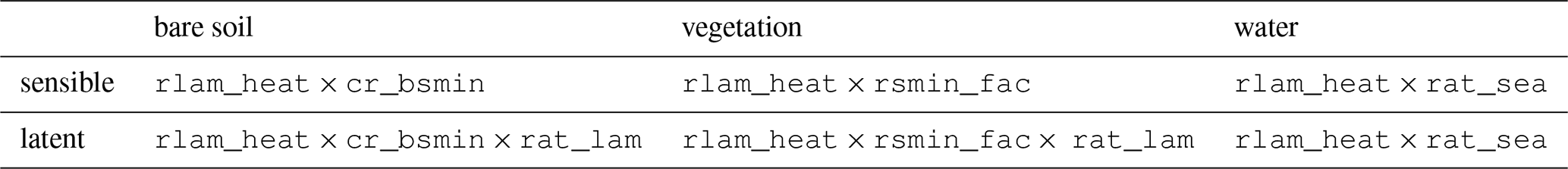
The main resistance parameter that scales both fluxes over land and water surfaces is rlam_heat. The parameter rat_sea is scaling the resistance of the fluxes over water. Here, the latent heat flux is equal to potential evaporation. The resistances and their scaling factors for vegetation, the land-use class-dependent evaporation/stomata resistance for plants are tunable by adjusting rsmin_fac. cr_bsmin is the tunable minimal bare soil resistance for evaporation. rat_lam influences the latent heat flux over land only.

All namelist parameters used are listed with a short description in Table A1.

2.2.3 New developments in parameterisation of sub-grid scale cloud cover

The ICON model includes three parameterisations that contribute to the simulated cloud cover. These encompass grid-scale cloud cover, subgrid-scale cloud cover from convection parametrisation, and subgrid-scale cloud cover from stratus or stratocumulus shallow clouds. The grid-scale cloud cover occurs when the grid-box relative humidity (rh) reaches 100 %. In this case, the cloud cover is automatically set to one, and the microphysics parameterisation is initiated, potentially producing precipitation. When rh is below 100 %, the grid-scale cloud cover remains zero. When the grid box rh is below 100 % but the stratification is unstable, the convection parameterisation is activated, and the cloud cover is estimated from the cloud water detained into the anvil (Bechtold et al., 2008). This cloud cover aims to describe shallow or penetrative cumulus, which may produce light to medium precipitation. The third cloud cover parameterisation is the subgrid-scale cloud cover of stratus or stratocumulus shallow clouds (Prill et al., 2024). When the grid-box mean rh is slightly below 100 % and subgrid-scale turbulent fluctuations are large enough, the grid box may contain small clouds (with rh of 100 %) and cloud-free areas with rh below 100 %. The turbulent fluctuations are parametrised using a top-hat total water distribution with a fixed half-width, which is around 5 % of the total water, which means that the water content varies uniformly within a narrow range around the mean value. This leads to a quadratic dependence of the subgrid-scale cloud cover on the total water.

The subgrid-scale cloud cover parametrisation due to turbulence is regarded as most uncertain, and therefore several parameters of the scheme are introduced as tuning parameters in ICON. The parameter tune_box_liq determines the half-width of the top-hat total water distribution. The parameter tune_box_liq_asy is a scaling factor that determines the asymmetry term of the cloud cover for over- and undersaturation. The quadratic increase of cloud cover from 0 to 1 ranges between rh_i and rh_f, where

$$\begin{array}{ll}\text{(2)}& {\displaystyle }& {\displaystyle }{\mathrm{\text{rh}}}_i=\mathrm{100}\cdot (\mathrm{1}-\mathrm{2}\cdot \mathtt{\text{tune\_box\_liq}}\cdot \mathtt{\text{tune\_box\_liq\_asy}}),{\displaystyle }& {\displaystyle }{\mathrm{\text{rh}}}_f=\mathrm{100}\cdot (\mathrm{1}+\mathrm{2}\cdot \mathtt{\text{tune\_box\_liq}}).\end{array}$$

In practice, since rh is not allowed to exceed 100 %, the cloud cover is cut off and does not reach 1 at rh=100 %. With higher tune_box_liq or tune_box_liq_asy, the quadratic increase of cloud cover starts at lower rh_i, resulting in higher cloud cover. However, the increase of tune_box_liq_asy leads to the increase of cloud cover for the entire range between rh_i and rh=100 %, while the increase of tune_box_liq does not change the value of the cloud cover at rh=100 %. Therefore, a higher sensitivity is expected to tune_box_liq_asy in comparison to tune_box_liq. Practically, the increase of cloud cover at lower rh is reflected in larger areas covered by partial cloudiness.

Finally, the scaling parameter allow_overcast determines the steepness of the parabolic function. Its decrease increases the steepness, preserving rh_i. As a result, a lower allow_overcast results in a higher cloud cover, especially at rh close to 100 %. This increase is reflected in the appearance of local spots with full overcast.

We used the ICON namelist parameter allow_overcast with a newly introduced monthly dependency. This change was inspired by the identification of monthly variations in model errors through a detailed analysis of test simulations. Technically, we simulated in monthly chunks and passed the appropriate monthly value to the namelist. It is defined for the month m as the mean value ao with added user-defined deviations from the mean aoac, scaled with a tunable amplitude aoa:

$$\begin{array}{}\text{(3)}& \mathtt{allow}\mathtt{\_}\mathtt{overcast}\left[m\right]=\mathrm{ao}+\mathrm{aoa}\cdot \mathbf{\text{aoac}}\left[m\right].\end{array}$$

Since this parameterisation does not include precipitation production, the described parameters affect the simulated radiation transfer through the clouds only. Therefore, their tuning is useful for correcting global radiation biases related to uncertainties in subgrid-scale cloud cover.

2.3 ICON-CLM model setup

This section provides an overview of our specific settings for this study. First, we provide a general description of the setup of ICON-CLM (Sect. 2.3.1), followed by an explanation of the design and naming conventions of the experiments in this study (Sect. 2.3.2). A special focus is put on the transient forcing of aerosol and ozone and the time-dependent insolation in Sect. 2.3.3.

2.3.1 ICON-CLM basic model setup

The ICON-CLM model domain for this study is the EURO-CORDEX region. The horizontal grid resolution is R13B5 in ICON terminology, which equals a mesh size of 12.14 km (Fig. S1 in the Supplement). Vertically, a hybrid height-based terrain-following coordinate (Smooth LEvel VErtical (SLEVE) coordinate;  Schär et al., 2002) is used with 60 layers up to a model top of 23.5 km. We use a model time step for advection of 100 s. In this study, ICON-CLM is driven by 3-hourly ERA5 reanalysis data (Hersbach et al., 2020). In previous tests (Sieck et al., 2026), it became obvious that an upper-boundary nudging towards the ERA5 data was beneficial for the European model domain due to the very large extension of the domain: The centre points of the western and the eastern boundaries are more than 7000 km apart. During the transition between summer and winter, high and low-pressure systems develop and travel across Europe at a high frequency. The nudging communicates these developments to the regional model and avoids strong boundary effects. It is applied above a height of 10.5 km to the horizontal wind components and additionally to the density and the virtual potential temperature using pressure, temperature, and specific humidity of ERA5. The nudging coefficient is maximum (i.e., =1) at the uppermost level and decreases to <0.5 in the third model layer from the top (full level height of 18.87 km), <0.25 in the fifth (at 16.34 km height), and <0.1 in the ninth (14.06 km).

At the ocean surface, ICON-CLM is using interpolated sea surface temperatures and sea ice fraction from ERA5. All boundary data are updated every three hours.

The ICON model provides different functionalities for the temporal aggregation of output variables and for vertical interpolation. We use the aggregation typical for climate variables and the interpolation to pressure levels and levels of constant height above mean sea level. ICON-CLM is running in a scripting framework or workflow engine, the so-called Starter Package for ICON-CLM Experiments (SPICE, Geyer et al., 2025a). The workflow consists of a parallel pre-processing of the lateral boundary conditions, the ICON-CLM simulation itself, post-processing, and archiving. The post-processing includes the interpolation of model output from the R13B5 ICON grid to the rotated EUR-12 grid and the generation of time series, the interpolation to constant heights above ground, and the calculation of typical climate variables like potential evapotranspiration, which are not directly diagnosed within ICON.

2.3.2 Reference simulation and study design

The reference simulation is the experiment C2I101 (Geyer et al., 2025c, reference configuration for experiments listed in Table C1). It is using the general setup as described in Sect. 2.3.1 and the physical parameterisations as described in Sect. 2.2.1, apart from the urban parametrisation TERRA_URB. As external parameters, GLOBE orography data (GLOBE Task Team et al., 1999), FAO soil types (Food and Agriculture Organization of the United Nations, 2003), land-use data from GLOBCOVER2009 (European Space Agency and Université Catholique de Louvain, 2010), monthly varying Tegen aerosols (Tegen et al., 1997), and MODIS surface albedo (Schaaf and Wang, 2021) for different wavelength bands were used. Spectral solar irradiance (Coddington et al., 2016) and ozone data (Global and regional Earth-system Monitoring using Satellite and in-situ data project (GEMS) climatology merged with data by the project “Monitoring Atmospheric Composition and Climate” (MACC), Inness et al., 2009, 2015) were prescribed as in the default NWP setup for global applications. These settings constitute the reference configuration (Fig. 1, stage 1g) for all experiments conducted in the definition phase of a new reference, where we mainly tested the external datasets, existing alternative parametrisations, and a group of parameters. Table A1 provides an overview of the tested parameters along with their descriptions, while Table C1 details the specific modifications applied in each experiment, identified by IDs ranging from C2I101 to C2I130. Here, all simulations were conducted for the period 1979–1984, with the period 1980–1984 used for model evaluation and shown in the figures with seasonal means. The initial year served as a spin-up period to allow the system to reach a quasi-equilibrium state (Table B1). An alternative initialisation with soil moisture from a longer spin-up experiment is available among the sensitivity experiments.

The new reference was defined as (C2I200/C2I200c) according to the tuning strategy (Fig. 1, stage 2g), using new settings as for example, transient aerosols (cf. Sect. 3.3 and Table D1 for more details). For the tuning process, a second time period, 2002–2008, was used (experiment IDs C2I2**c). The period from 2003 to 2008 was used for the evaluation and tuning, and the figures refer to the seasonal means obtained from this period. This second period was added to increase the number of available observational data, as sufficient satellite data are not available in earlier times. Optimised LiMMo configurations were tested in experiments C2I291c and C2I294c (cf.  tuning strategy step 4f). The ICON namelist parameters and the simulation acronyms are written in the manuscript with font typewriter.

Since the tuning initiative took place at the same time as the development of the ICON source code, the model version was changed several times during the process (see Table B2).

2.3.3 Transient Forcing

The settings for the transient forcing of aerosol and ozone and the time-dependent insolation were gradually adopted from the ICON setup for coupled global climate projections, ICON-XPP, (Müller et al., 2025); see experiments C2I105, C2I118, C2I119 (Table C1) for a description of the respective ICON settings. The implementations were adopted from a predecessor of ICON-XPP, called ICON-ESM (Jungclaus et al., 2022), which are in turn very similar to those in the atmospheric part of the general circulation model by the Max-Planck-Institute, ECHAM-6 (Stevens et al., 2013). The main development had to be invested into the treatment of the input parameters provided by these climatologies, which required adaptations in the radiation interface for ecRad. For the aerosols, the input of the transient “Max Planck Aerosol Climatology Version 2” (MACv2) of Kinne (2019a) is implemented, with the option to use the simple plume scheme MACv2-SP of Stevens et al. (2017). Only the simple plume scheme includes the option to account for different aerosol concentrations in dependence on the respective climate scenario. As the optimised setup described in this article will also be used to downscale GCM simulations for different scenarios, the simple plume scheme must be used. Additionally, a transient climatology for volcanic aerosols (Stenchikov et al., 1998) can be read. For ozone, the CMIP6 dataset (Checa-Garcia, 2018) was made available. Moreover, an option to switch on time-dependent spectral solar irradiance as recommended for CMIP6 (Matthes et al., 2017) is available.

Due to the switch from the Tegen aerosol climatology to the transient MACv2-SP climatology, the aerosol-microphysics coupling as used in NWP is not applicable anymore. Therefore, the use of an external MODIS climatology of cloud droplet number concentration (CDNC) was implemented for ICON-XPP, which is tested in C2I241 (see Table D1). The current implementation uses a non-transient, but monthly varying climatology of Gryspeerdt et al. (2022) and was adjusted with a satellite-based CDNC retrieval by Bennartz and Rausch (2017) and Grosvenor et al. (2018) as used in ECMWF's IFS model. To account for the scenario-dependence of aerosols and, with that, of CDNCs, we implemented a scaling factor that can be derived from the implementation of the simple plume scheme (Fiedler et al., 2019). This implementation is not tested for the periods considered here, but will be used for the production of RCM scenarios.

2.4 LiMMo framework

Figure 1 (Stage 4: LiMMo Tuning) briefly describes the meta-model-based tuning framework developed and applied in the current study (Petrov et al., 2025). This framework is very useful for leveraging sensitivity simulations (Fig. 1, stage 2c) and adds significant value to the process of finding the optimal model configuration. The first stage of meta-model-based tuning involves statistically approximating the monthly mean climate model output and building (or training) a meta-model, or emulator (Fig. 1(4a)). The next stage is the optimisation loop (Fig. 1(4b–d)). At this stage, the user selects the weights of the model variables in order to scale the terms of the error norm function, which quantifies the discrepancy between the meta-model and the observational data (Fig. 1(4b)). Then, the optimisation procedure is conducted to yield the parameter values that minimise the error norm function (Fig. 1(4c)). Then, the user checks whether the meta-model's biases with optimal parameter values fulfil the global tuning aim (Fig. 1(4d)). If so, a control test run of the climate model is conducted to confirm the findings. (Fig. 1(4f)).

In this section, we give the general description of the framework (Sect. 2.4.1) and present the error norm function that guides an optimisation (Sect. 2.4.2).

2.4.1 General description

The meta-model framework has two distinctive features: first, a linear regression emulator, and second, gradient-based optimisation of meta-model parameters to minimise the error norm between the emulator and the observations.

Unlike previous studies, which mainly utilised quadratic regression (Gregoire et al., 2011; Bellprat et al., 2016), the LiMMo concept has successfully proven that linear approximation possesses decent approximation quality for multi-year monthly mean values, requiring only a linear number of simulations (for N parameters, the number of simulations required for training is O(N)). Contrary to this, the quadratic regression requires O(N²) simulations, because one has to conduct one new simulation with every two parameters disturbed simultaneously to approximate the interaction terms. This imposes a significant limitation on the number of parameters available for tuning.

The linear regression REG(p) defined in the following equation is a function of the model parameters p and approximates ICON-CLM variables. The regression yields monthly mean values, which correspond to the climatological monthly means (average December, January, etc.):

$$\begin{array}{}\text{(4)}& {\displaystyle }{\text{REG}}_{i,j,k,n}\left(\mathit{p}\right)={\text{MOD}}_{\text{ref}}^{i,j,k,n}+\sum _m(p_m-p_m^{\text{ref}})\cdot {\mathbf{K}}_{i,j,k,n}^m.\end{array}$$

Here, ${\text{REG}}_{i,j,k,n}$ is the 2D regression result ((i,j) are spatial indices, k is the number of the climatological month, and n is the index of the model variable), ${\text{MOD}}_{\text{ref}}^{i,j,k,n}$ is the model output for the reference simulation, p_m and $p_m^{\text{ref}}$ are the test parameter and reference parameter values for the parameter with index m (corresponding to MOD^ref), and ${\mathbf{K}}_{i,j,k,n}^m$ is the tendency tensor of the parameter p_m. The tendency tensor is assembled explicitly as the linear combination of simulations (see Table 5, column “signal”), divided by the parameter increment (see Table 5, columns “test value” and “ref value”). Note that the regression in Eq. (4) is constructed to be exact for the reference parameter values.

To start the experiments with the meta-model, we select the error norm function ERR(p), which sets the distance between meta-model (Eq. 4) and observational data. We give the details of the error norm function in the following section (Sect. 2.4.2). Mathematically, the aim of the meta-model tuning is to find the vector of model parameters p that would minimise the ERR(p).

For the linear regression approximation with a spatial RMSE-based error norm, the target minimisation function ERR(p) is a smooth, convex, scaled Euclidean norm function of the model parameters. This function is known to have only one global minimum. Consequently, the initial parameter values have no impact on the outcome, and the optimisation process always converges to the global minimum. However, this minimum may be on the boundary of the constrained region for certain parameters. This, however, should not be the case for physically consistent parameters and physically meaningful parameter ranges of parameter values admitted. Section 3.4.2 will show that this was not the case for the parameters optimised in this study.

In previous studies devoted to objective calibration (e.g., Bellprat et al., 2016; Avgoustoglou et al., 2022), Monte Carlo sampling was utilised for this purpose. The general problem of this approach is the exponentially growing complexity with the dimensionality of the parameter space N, which in practice limits N. In previous studies, N was limited to 7–8 parameters.

In the LiMMo framework, the Monte Carlo method is applied to binary parameters (logical and integer value parameters). The number of these parameters can be significantly higher due to the very fast solution of the linear model. Thus, more sophisticated methods are not necessary to solve this type of problem within a few hours.

For real number parameters, the LiMMo framework suggests the implementation of gradient-based optimisation. This method searches for the next value of the parameter vector ${\mathit{p}}^n\to {\mathit{p}}^{n+\mathrm{1}}$ in the direction opposite to the gradient of the error norm in the parameter space $\left(\partial \text{ERR}\left(\mathit{p}\right)/\partial \mathit{p}\right)$, until the increment of the error norm function becomes less than a given threshold $\left|\text{ERR}\left({\mathit{p}}^{n+\mathrm{1}}\right)-\text{ERR}\left({\mathit{p}}^n\right)\right|<\mathit{\epsilon }$. As proposed by Petrov et al. (2025), the limited-memory Broyden-Fletcher-Goldfarb-Shanno method (Broyden, 1970; Byrd et al., 1995) with box constraints fits really well to the purpose and the convex nature of the problem. This method requires an initial guess and the minimum and maximum parameter values $p_m^{\text{min}}$ and $p_m^{\text{max}}$ to set up the box constraints. The search process is restricted to the defined hyper-rectangle, which ensures that the final result is physically meaningful. The complexity of gradient descent increases linearly with the dimensionality of the parameter space. In practice, an optimisation with 15–20 parameters is in the order of a few minutes only.

We successfully built a regression meta-model with over 15 parameters and ran multiple optimisation loops (see Sect. 3.4.2). As a result, we obtained several parameter sets derived from LiMMo as final contenders for the new, optimised ICON-CLM configuration.

2.4.2 Error norm

In the LiMMo framework, the error norm (single number) between the model output and observational data is calculated using the Root Mean Square Error (RMSE). The observational data are first interpolated onto the model's output grid. Then, multi-year monthly averages were computed for both the model output and the observational time series.

To compute the error norm, we consider the horizontal model outputs ${\text{MOD}}_{i,j,k,n}$ for the variables v_n. The indices i and j represent the spatial coordinates on the horizontal grid, while k indicates the month. The observational data ${\text{OBS}}_{i,j,k,n}$ are stored in the same multi-year monthly mean manner on the model grid.

The spatially aggregated Root Mean Square Error, RMSE_k,n, for each month and variable is given by

$$\begin{array}{}\text{(5)}& {\displaystyle }{\text{RMSE}}_{k,n}=\sqrt{{\displaystyle \frac{\mathrm{1}}{N_x\cdot N_y}}\sum _{i,j}{\left({\text{MOD}}_{i,j,k,n}-{\text{OBS}}_{i,j,k,n}\right)}^{\mathrm{2}}},\end{array}$$

where N_x⋅N_y denotes the number of grid points on the horizontal plane of the simulation domain, excluding the boundary relaxation zones. For each variable and month, the intrinsic variability σ_k,n is defined as the RMSE between some reference and its disturbance simulation. In our case, the disturbance is achieved by shifting the initial conditions back by one month:

$$\begin{array}{}\text{(6)}& {\displaystyle }{\mathit{\sigma }}_{k,n}=\sqrt{{\displaystyle \frac{\mathrm{1}}{N_x\cdot N_y}}\sum _{i,j}{\left({\text{MOD}}_{\text{ref}}^{i,j,k,n}-{\text{MOD}}_{\text{dis}}^{i,j,k,n}\right)}^{\mathrm{2}}}.\end{array}$$

The error ERR_n for each variable is calculated as the time-averaged RMSE normalised by the intrinsic variability, defining the dimensionless signal-to-noise type measure of model prediction quality with respect to observations:

$$\begin{array}{}\text{(7)}& {\displaystyle }{\text{ERR}}_n={\displaystyle \frac{\mathrm{1}}{N_t}}\sum _k{\displaystyle \frac{{\text{RMSE}}_{k,n}}{{\mathit{\sigma }}_{k,n}}},\end{array}$$

where N_t=12 represents the number of months. Finally, the total error norm, ERR, is defined as the weighted sum of the errors for each variable, which determines the aggregated quality of the model simulation for all the prognostic variables that have been considered:

$$\begin{array}{}\text{(8)}& {\displaystyle }\text{ERR}=\sum _n{c}_n\cdot {\text{ERR}}_n,\sum _n{c}_n=\mathrm{1}.\end{array}$$

The weights c_n are chosen by the user to reflect the relative importance of each variable, directly controlled by the optimisation aim (Fig. 1(1d); see Sect. 3.4.2). The aim of LiMMo tuning is to minimise this error norm (Eq. 8) with respect to the model parameters.

2.5 Observational Datasets and analysed variables

The single-level 2D model variables considered in the evaluation and tuning procedure are listed in Table 2. We use the EURO-CORDEX naming convention (EURO-CORDEX, 2025) to label them. Multiple gridded data sets are used for ScoPI score analysis (see Sect. 2.6.1), LiMMo tuning (see Sect. 2.4.2), and/or comparison with station observations. We will use bold font to emphasise the model variables in the following text.

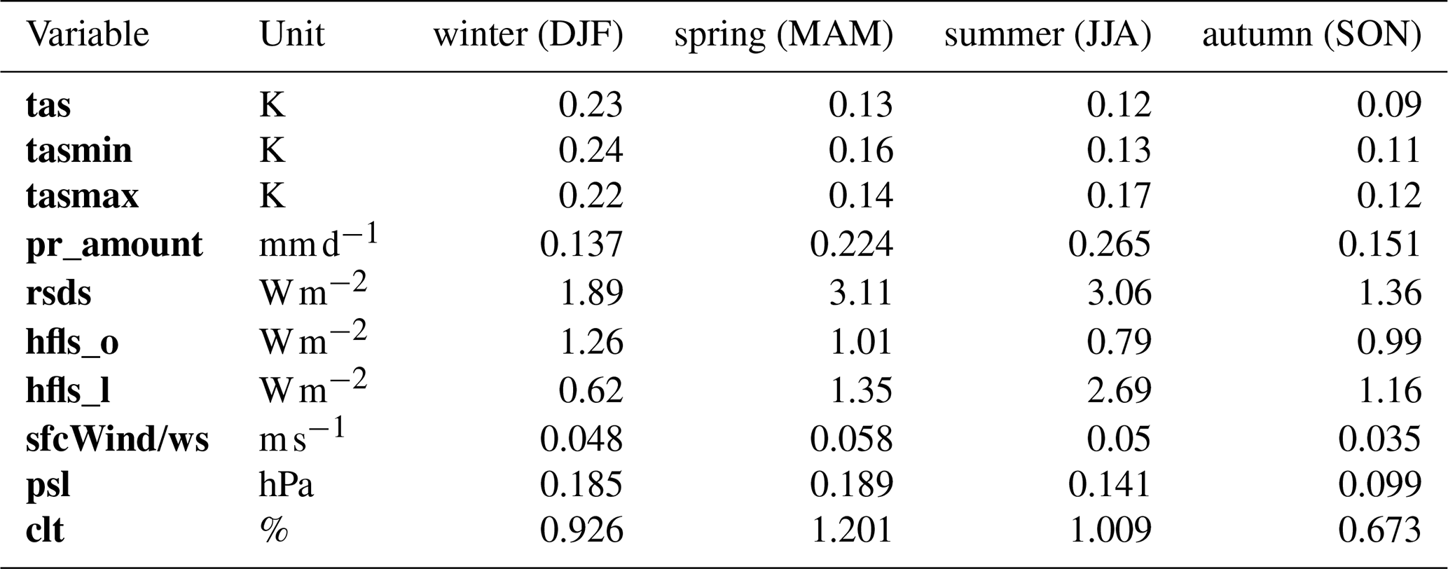
Table 2 List of considered model variables comprising the variable name according to the EURO-CORDEX convention, a short description, and the respective unit. If the variable is analysed or tuned against observations, the corresponding data source is provided and explained in the main text; “–” indicates that no comparison with observations was done. In addition, the weight of the variable in the ScoPi-score metric (Sect. 2.6.1) is given.

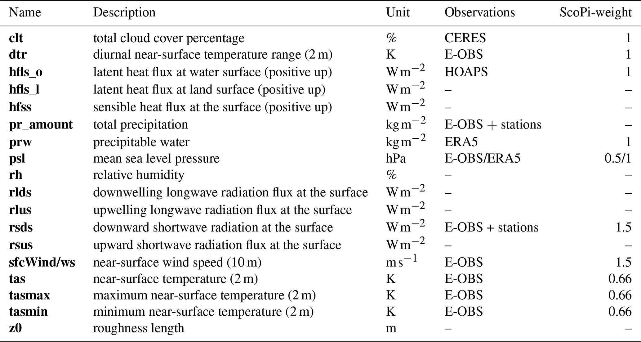
For the evaluation of the model results, detailed comparisons against the gridded observational data set E-OBS version 29 (Cornes et al., 2018) were conducted. Daily data were retrieved on a regular grid with a spatial resolution of ∼ 25 km. Additionally, satellite data are used for the 2003–2008 evaluation period, namely HOAPS 4.0 (Andersson et al., 2010, 2017) and CERES (NASA/LARC/SD/ASDC, 2019; Loeb et al., 2018) as monthly mean composites. The variables considered in the evaluation procedure are listed in Table 2.

Additionally, precipitation and radiation observations from weather stations in Germany (Deutscher Wetterdienst, 2025) and Poland (Polish Meteorological Service) for 2004 to 2008 were used for the evaluation of the surface energy budget components.

2.6 Evaluation Procedure and Considered Metrics

In a first instance, the evaluation is conducted point-by-point on the regular lon-lat grid of the selected observational data set for at least 5 years. Beforehand, simulation data were remapped to the observational grid using bilinear interpolation. The main metrics that we consider in our analyses are the following: mean error (mean BIAS), RMSE, Linear Correlation in time, and the Advanced (symmetric) Mean Squared Error Skill Score (AMSESS), defined after Winterfeldt et al. (2011), see Eq. 9.

$$\begin{array}{}\text{(9)}& \text{AMSESS}=\left\{\begin{array}{ll}\mathrm{1}-{\mathit{\sigma }}_{\mathrm{ts}}^{\mathrm{2}}\cdot {\mathit{\sigma }}_{\text{ref}}^{-\mathrm{2}}& \text{if }{\mathit{\sigma }}_{\mathrm{ts}}^{\mathrm{2}}\le {\mathit{\sigma }}_{\text{ref}}^{\mathrm{2}}\\ {\mathit{\sigma }}_{\text{ref}}^{\mathrm{2}}\cdot {\mathit{\sigma }}_{\mathrm{ts}}^{-\mathrm{2}}-\mathrm{1}& \text{if }{\mathit{\sigma }}_{\mathrm{ts}}^{\mathrm{2}}>{\mathit{\sigma }}_{\text{ref}}^{\mathrm{2}}\end{array}\right.,\end{array}$$

where σ_ts and σ_ref are the mean squared differences of the test and reference simulations against observations, respectively. The AMSESS varies between −1 and 1, where positive (negative) values indicate improved (worsened) performance of the test simulation with respect to the reference.

We compare the model error against the observations of a given simulation and the respective reference runs for each variable and grid-box, based on the aforementioned metrics. The error of a given simulation against observations might be smaller or larger than the one of the reference run. However, whether these smaller or larger errors are significant must be tested. In the next section, we present a method for making a statistically sound assessment of whether a given simulation is better or worse than the reference in the comparison against observations.

2.6.1 Significance tests and Score Points of evidence – ScoPi

For the significance tests and Score Points of evidence (ScoPi) we followed the approach introduced by Geyer (2026). The ScoPi is calculated point-by-point, considering the 3-daily means or sums, respectively, of the given variables (Table 2). Given that the ERA5 data, used as boundary conditions for the conducted experiments, are “realistic” reanalysis data, we assume that the model can adequately capture the variability of a given variable at synoptic time scales within a single grid cell. This enables, on the one hand, having a time series long enough for testing the robustness of the employed metrics using Monte-Carlo approaches. On the other hand, it allows for making the variables more Gaussian through averaging: this then allows for the application of estimators such as the RMSE, which are better suited for normally distributed data (Hodson, 2022). For CERES cloud cover, monthly mean values are considered instead of 3-daily means, representing the original temporal resolution of the CERES data set. When applying the LiMMo, monthly mean values of the variables are used.

The ScoPi score is described in detail by Geyer (2026). It is dependent on the shares of grid points in a model sub-region, presenting a significant improvement or worsening in a metric for a variable with respect to the reference run. If the share of grid points in a model region with a strong (not only moderate) significance F_ss is larger than 0.5, the score is enlarged by 0.5 as given in Eq. 10, F_ms denotes the shares with moderate significance.

$$\begin{array}{}\text{(10)}& \text{ScoPi}=\left\{\begin{array}{ll}{F}_{\mathrm{ss}}+\mathrm{0.5}\cdot \mathrm{sign}\left(F_{\mathrm{ss}}\right)& \text{if }\left|F_{\mathrm{ss}}\right|>\mathrm{0.5}\\ F_{\mathrm{ms}}& \text{otherwise}\end{array}\right.\end{array}$$

The great advantage of the ScoPi score is its inherent standardisation for different types of variables. The values always range between −1.5 and 1.5. Therefore, the ScoPi score can be aggregated over different types of variables and metrics. The inspection of these values allows us to gain a comprehensive understanding of the reasons for possible improvement/worsening in the model performance for a given configuration. The ScoPi score is computed for each PRUDENCE region (see Fig. S1), for different metrics m, seasons s, and various atmospheric variables v. If the share of significant grid points in a sub-region is too small (lower than 0.4), the ScoPi score is not accounted for when aggregated. In this case, it is assumed that there is no noticeable large-scale change in the model results with respect to the reference. The aggregation with respect to a specific PRUDENCE region is done by calculating the sum over the ScoPi values for all seasons, metrics, and variables (Eq. 11). For integrating over several variables, different weights c_v are considered per variable, as given in Table 2. The resulting value is referred to as ScoPi_region.

$$\begin{array}{}\text{(11)}& \begin{array}{rl}& {\text{ScoPi}}_{\mathrm{region}}\left(r\right)\\ & =\sum _{v,m,s}{\text{c}}_v{\text{ScoPi}}_{v,m,s}\left(r\right)\mathbf{1}\left(\left|{\text{ScoPi}}_{v,m,s}\right(r\left)\right|>\mathrm{0.4}\right),\end{array}\end{array}$$

where $\mathbf{1}\left(\left|{\text{ScoPi}}_{v,m,s}\right(r\left)\right|>\mathrm{0.4}\right)$ is the indicator function giving 1 for ScoPis larger/smaller than $\mathrm{0.4}/-\mathrm{0.4}$ and 0 elsewhere.

The threshold of 0.4 ensures that the majority of the locations in a specific region and for a specific model configuration show a significant improvement/worsening compared to the reference experiment. For instance, if at least 40 % of the grid points show significantly improved performance for simulation B with respect to reference A, the ScoPi score is 0.4, although 60 % of the grid points show no significant changes. The same is true if 60 % of the grid points show significant improvement and 20 % significant worsening.

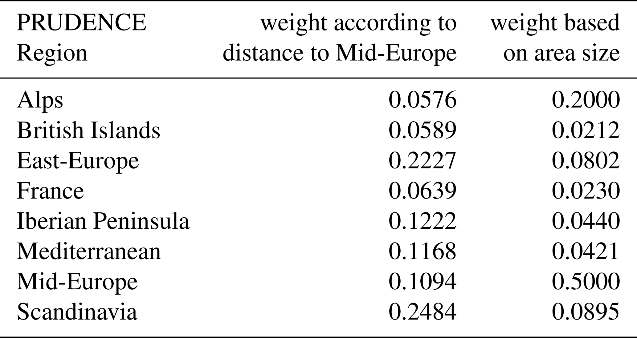
ScoPi_simulation is defined as a weighted sum across all PRUDENCE regions, incorporating additional regional weighting factors (Eq. 12). Each PRUDENCE region is assigned a specific weight, based either on its area or its distance from mid-Europe (domain A4 in Fig. S1). The corresponding weights are listed in Table 3.

$$\begin{array}{}\text{(12)}& {\text{ScoPi}}_{\mathrm{simulation}}=\sum _r{\text{c}}_r\cdot {\text{ScoPi}}_{\mathrm{region}}\left(r\right),\end{array}$$

To calculate a ScoPi_simulation, it is a prerequisite that each contributing region is analysed with the same set of metrics and variables. Therefore, it is not possible to summarise regions' results for different variables, i.e., temperatures for land points of PRUDENCE regions and latent heat fluxes of sea points.

Table 3 ScoPi weights according to the region area (middle) or to distance from the domain centre (Germany) (right).

The ScoPi is calculated in a first place considering the mean BIAS against observations for all of the given variables. Then, it is also applied to the other metrics mentioned above. When applying the error metric “linear correlation”, we used the method proposed by Zou (2007) and described in Geyer et al. (2025a) as a significance test for the differences between two simulations. Tests with several metrics done by Geyer (2026) revealed that the ranking between the tested simulations remains stable in relation to the reference: the higher the ScoPi score, the better the overall performance of the tested simulation.

2.6.2 Sensitivity measure

To quantitatively compare the impact of different parameter changes on model results and to help in the selection of parameters, which are worth considering for further tuning, we introduce the sensitivity measure ${\text{SENS}}_{n,m}^{\text{seas}}$ for variable v_n on the change of parameter p_m for a specific season (seas). Each sensitivity experiment simulates the change of only one parameter from the reference value $p_m^{\text{ref}}$ by an increment of Δp_m. The definition of the sensitivity measure is comparable to the definition of the error norm with respect to observations (Eq. 7):

$$\begin{array}{}\text{(13)}& \begin{array}{rl}& {\text{SENS}}_{n,m}^{\text{seas}}={\displaystyle \frac{\mathrm{1}}{N_{\text{seas}}}}\cdot \sum _{k\in \text{seas}}{\displaystyle \frac{\mathrm{1}}{{\mathit{\sigma }}_{k,n}}}\\ & \cdot \sqrt{{\displaystyle \frac{\mathrm{1}}{N_x\cdot N_y}}\cdot \sum _{i,j}{\left({\text{MOD}}_{i,j,k,n}^{p_m=p_m^{\text{ref}}+\mathrm{\Delta }{p}_m}-{\text{MOD}}_{i,j,k,n}^{p_m=p_m^{\text{ref}}}\right)}^{\mathrm{2}}},\end{array}\end{array}$$

where N_seas is the number of months in a specific season, σ_k,n is the intrinsic variability of variable v_n for the month number k (Eq. 6), N_x,N_y are the number of grid points along the domain axes, ${\text{MOD}}_{i,j,k,n}$ is the ICON-CLM model output temporally averaged to monthly mean values for several years (i,j – spatial indices, k is the index of month, n is the index of model variable).

In addition, we applied a grid point mask to the model quantities before calculating the sensitivities, using only the grid points with available observations (E-OBS for all variables except hfls_o, and HOAPS for hfls_o). This shows the sensitivity only for the relevant part of the model domain.

Within a physically meaningful range of parameters, the sensitivity can be treated as a signal-to-noise ratio. The signal is the RMS difference between the model outputs for the reference configuration and the configuration with the parameter disturbed. The noise is the intrinsic variability of the model. Therefore, statistically significant changes yield a sensitivity value greater than 1. We consider the model to be “sensitive” to a parameter change for SENS^seas values above 2.

3 Results

In the results section, we present the sensitivity study and parameter tuning outcomes for ICON-CLM. This section is organised according to the proposed RCM tuning strategy (Fig. 1). First, we determined the intrinsic variabilities of the model for the analysed variables (Sect. 3.1). In Sect. 3.2, we investigate how key model quantities respond to changes in 27 tested model parameters. For those parameters that turned out to show a high sensitivity, we discuss 2D seasonal signals that provide valuable insights into the model's behaviour. In Sect. 3.3, we propose a new reference configuration that uses settings which were found to most effectively improve model quality during the sensitivity study, unless they must be changed for scientific reasons. We also examine the primary biases of the new reference configuration to observations to determine the tuning aim. In Sect. 3.4, the results of the expert- and meta-model-based tuning are presented. Finally, in Sect. 3.5, we carefully evaluate all configurations obtained. One optimum configuration is recommended with respect to simulation quality and computational efficiency, to be used as the new recommended reference configuration for 12 km climate runs over Europe within the CLM-Community.

3.1 Intrinsic variability

One requirement of the tuning strategy is to determine the monthly mean intrinsic variability of the modelled quantities (see Fig. 1(1b) and Sect. 2.4.2), which are used to estimate the model sensitivity. The seasonal mean values are given in Table 4. These values are also used to determine uncertainty ranges during evaluation and tuning processes, as well as the minimum range displayed in seasonal 2D bias plots.

Table 4 The seasonal values of intrinsic variability measure, computed as RMS difference between simulations C2I207 and C2I200 (see Eq. (6) and Table D1). The observation mask is applied to the model output (only the grid points where observations are available take part in the computation).

3.2 Parameter testing for ICON in Climate Mode

During the parameter testing phase (stage 2 of the RCM tuning strategy, see loop 2b–2e in Fig. 1), we divided all model runs into two groups: Tables 5 and 6 provide an overview of the parameter changes tested and how the change signals, i.e., the impacts of the parameter adjustments or changes, were calculated. In this section, we investigate these signals for those model quantities, i.e., model outputs, that show the largest sensitivity to parameter changes. The first group consists mainly of the external input data sets and parameters related to the configurations of the soil and vegetation, cloud, and convection parameterisations (see Table 5) used for the definition of the new reference. In the second group, we tested the sensitivity of disturbed values of continuous parameters (Table 6) for later use in either the expert tuning mode or the LiMMo optimisation (see Sect. 3.4).

Table 5 Parameters tested for the definition of a new reference, the selection is based on expert knowledge. “reference values” indicate the settings of the reference experiment. The meaning of the abbreviated parameter values marked with an asterisk “^*” is explained in Table A2. The “signal” column denotes the two simulation IDs (without “C2I” prefix) that are used to estimate the impact of parameter changes. These IDs are documented in Table C1. Parameters in a typewriter font are ICON namelist parameters, and parameters in bold correspond to multiple parameters changed simultaneously.

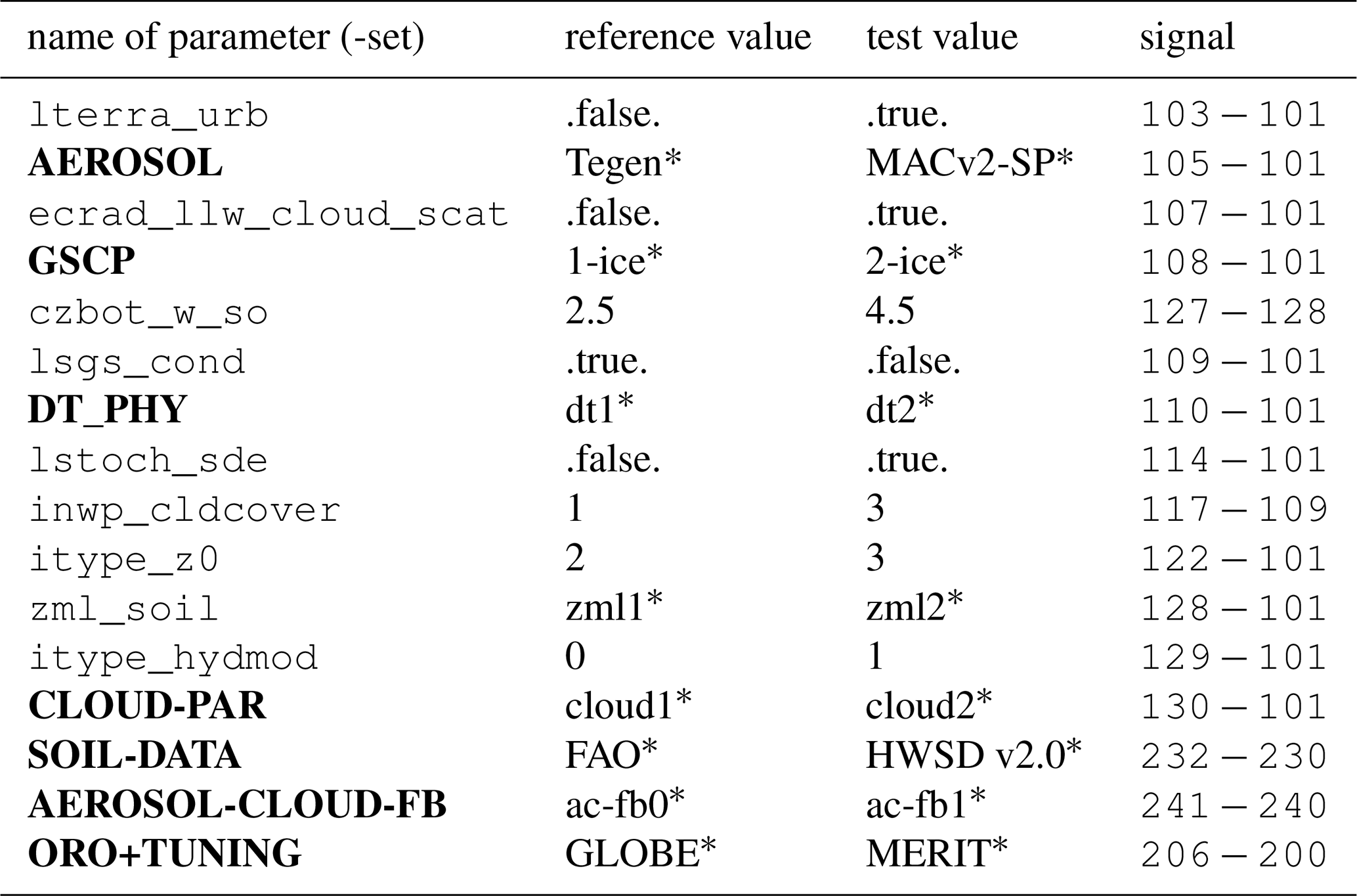
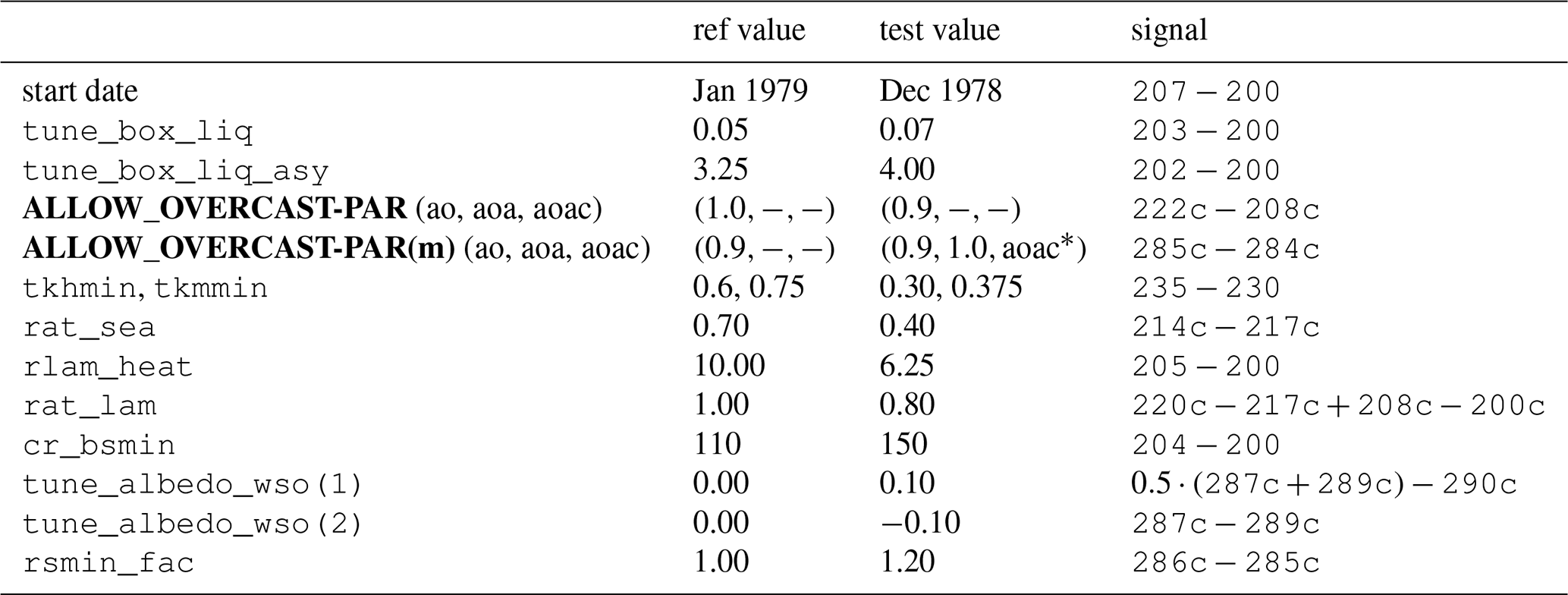
Table 6 As Table 5, but for parameters tested during the sensitivity study. Values marked with “^*” are explained in Table A2. The parametrisation of allow_overcast (ao, aoa, aoac) is explained in Eq. (3).

To systematically assess the impact of parameter changes on model quantities, we present the sensitivity measure values (see Eq. (13) in Sect. 2.6.2) for the winter and summer seasons in Fig. 2. The sensitivity tables show the sensitivities of the main surface model quantities (see Table 2) with respect to the modifications of the model parameters given in Tables 5 and 6. The parameters corresponding to the update of external datasets are shown separately in the upper panels of Fig. 2 as they are used for scientific reasons despite their sensitivity values.

We found no significant sensitivity in winter or summer for the following parameters: lterra_urb, AEROSOL-CLOUD-FB, ecrad_llw_cloud_scat, czbot_w_so, lsgs_cond, zml_soil, cr_bsmin, tune_albedo_wso(2), and rsmin_fac. Hence, we only discuss these parameters briefly and classify them as “not sensitive parameters”. The remaining parameters tested exhibit a sensitivity around twice the intrinsic variability or larger, especially during the summer, and are classified as “sensitive parameters”.

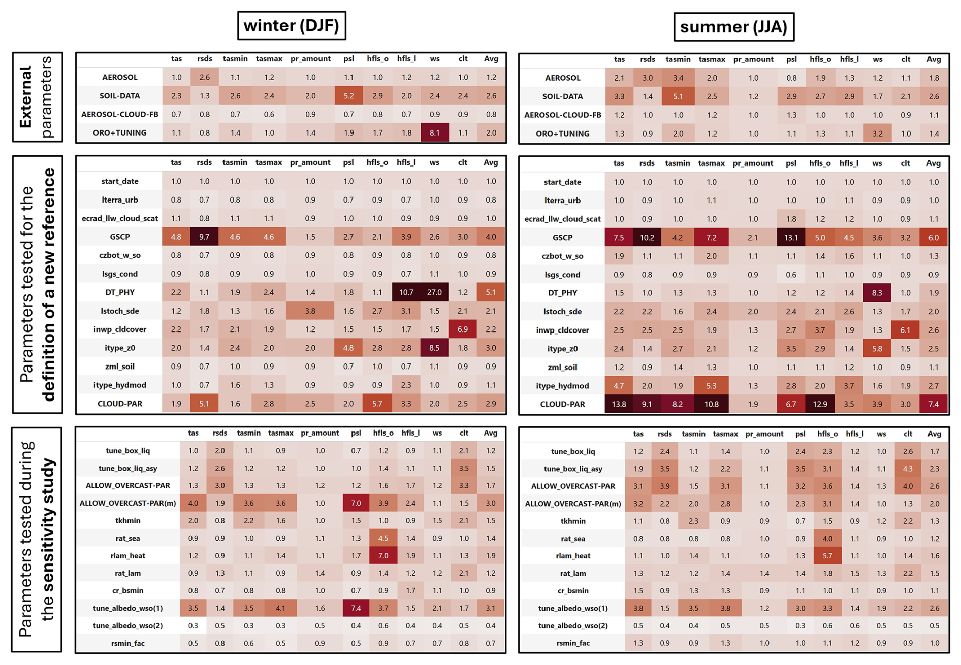
Figure 2 Mean seasonal sensitivities of the ICON-CLM to changes in tested parameters. In each table, the rows represent the model parameters and the columns the model quantities, where the last column “Avg” gives the average value. The tables on the left show the sensitivity values for the winter (DJF) season. The tables on the right show the sensitivity values for the summer (JJA) season. Sensitivities are shown for the external parameters (top row, see Table 5), for parameters tested for the definition of a new reference (centre row, see Table 5), and for the parameters tested during the sensitivity study (bottom row, see Table 6). The sensitivity measure is defined in Eq. (13). The intensity of the background increases with values (the same scaling for all tables).

For the remainder of this section, the impacts of changed sensitive parameters are systematically presented: Sect. 3.2.1 discusses the impact of changing external datasets. Section 3.2.2 presents parameters of surface and subsurface processes. Section 3.2.3 investigates the parameters controlling planetary boundary layer, mixing, and convection-related processes. Section 3.2.4 presents the signals for parameters of microphysics and cloud cover diagnostics.

3.2.1 External parameters

External parameters are static or monthly varying fields prescribed “externally” to the model and describe the physical properties of the environment. We replaced data sets of lower quality and/or resolution with those of higher quality and/or resolution. In the following, we discuss the impact of the parameter modification on model results. Where the simulation quality is discussed, we use E-OBS data as an observational reference. The sensitivities of the model to changes of the external parameters in winter and summer (see average values in Fig. 2) are large for soil type (“Avg” sens: DJF = 2.6, JJA = 2.6) and orography data (“Avg” sens: DJF = 2.0, JJA = 1.4), and minor for natural and anthropogenic aerosol (“Avg” sens: DJF = 1.2, JJA = 1.8), and aerosol-cloud-feedback (“Avg” sens: DJF = 0.8, JJA = 1.1). The summer tasmin is thereby the most sensitive variable. A configuration with the higher-quality external parameters is used later on as a new reference, C2I250c, for the parameter tuning.

Soil Data (test: HWSD v2.0*, reference: FAO*)

For the soil type distribution sensitivity experiment, we replaced the default FAO soil dataset (Food and Agriculture Organization of the United Nations, 2003) by the Harmonised World Soil Data Base version 2.0 (HWSD v2.0;  FAO and IIASA, 2023), see Fig. 3a and b. The HWSD v2.0 data have a much smaller typical length scale (4 to 7 km) in comparison with FAO (10 to 50 km) and show a higher frequency of sandy loam than loam soil types (Fig. 3 c).

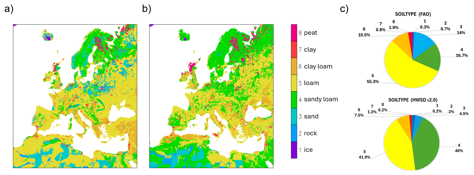
Figure 3 Default (operational) soil-type distribution based on the FAO (a) and HWSD v2.0 (b) datasets. The Pie chart (c) gives the portions of the spatial extent for soil types [in percent] shown in (a) and (b).

Figure 4 shows the impact of the systematic shift to more “sandy loam” soils on tas, hfss, and hfls in summer. Additionally, Fig. S2 gives the surface air pressure and the relation of sensible to latent heat flux (Bowen ratio). The shift increases the daily maximum temperature tasmax in central to eastern Europe and tasmin over the southern Iberian Peninsula and in northern Africa by up to 1 K. The change in tasmin is highly correlated with the Bowen ratio, in particular in regions with low hfls. The change in tasmax is strongly correlated with the absolute sensible heat flux hfss, in particular in central to eastern Europe and the Hungarian basin. Here we find a small change in the Bowen ratio since the latent heat flux is relatively high in these regions. Approximately, we find a change of temperature with forcing $\mathrm{d}T/\mathrm{d}F\simeq \mathrm{0.1}$ K m² W⁻¹.

A similar effect we found in Morocco and Algeria for soil types change from loam to loamy clay in the north. Consistently herewith, in areas of the Mediterranean region, where loamy clay is changed to loam (Adriatic coast, Po valley, Greece, and Turkey), we found the opposite in summer: an increase of hfls and a decrease of Bowen ratio. Interestingly, the same effect is found in regions of a change from loamy clay to clay (Sicily). In these regions, the loamy clay holds more plant-available water than clay and loam during the summer. While clay has a high total water holding capacity, a significant portion of that water is held very tightly and is hardly available for plant transpiration. The loamy soils are already dry in summer since the water evaporated and/or drained in previous months.

A similar phenomenon can be found for the shift from sand or loam to sandy loam in the region of northern Germany, Denmark, and Poland. Here, “sandy loam” exhibits the highest hfls.

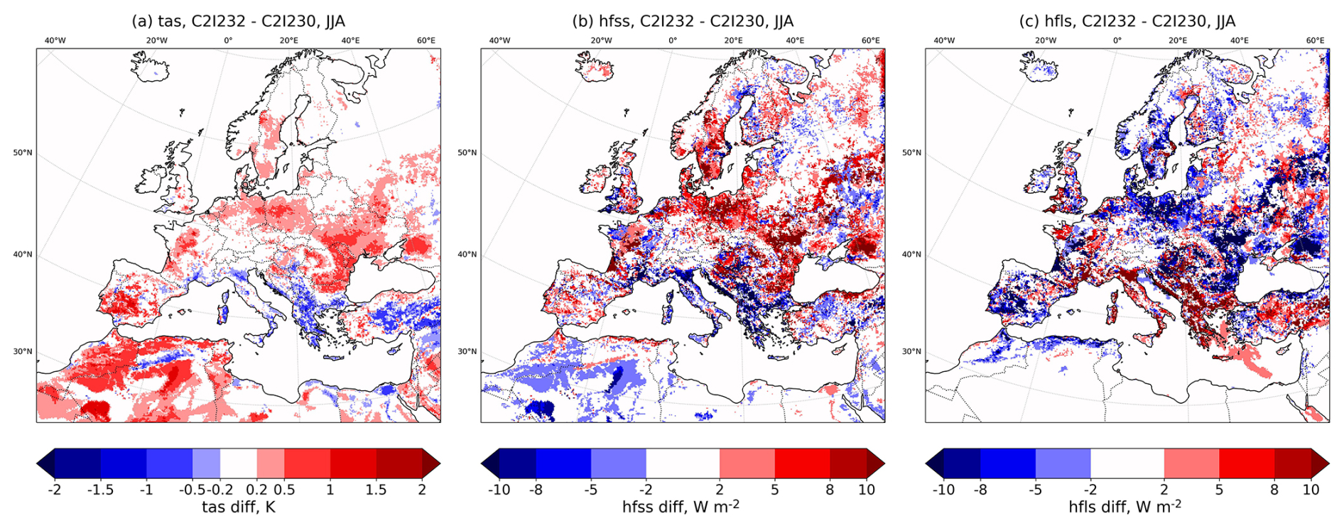
Figure 4 Sensitivity of ICON-CLM with respect to soil type distribution determined from HWSD v2.0 (test) and FAO (reference), soil_data. Mean differences for JJA 1980–1984 between test and reference as defined in Table 6 in column “signal” for tas (left), hfss (center), and hfls (right).

Orography data and related model tuning (test: MERIT*, reference: GLOBE*)

Using the updated model orography data set is accompanied by applying a set of revised tuning parameters for the sub-grid scale orography scheme (see settings of C2I206 in Table D1). Figure 5a shows the z0 of the GLOBE dataset based orography, while Fig. 5b indicates a strong increase in z0 over Sweden and north-eastern Russia when using orography data based on the Multi-Error-Removed Improved Terrain Digital elevation model (MERIT). The main effect is a reduction of sfcWind (10 m wind speed) (Fig. 6) by 0.5 to 1.0 m s⁻¹ on average due to a combined effect of subgrid-scale orography scheme and the direct effect of increased surface roughness, this means a reduction of the model bias compared to E-OBS (Fig. 6). The changes of subgrid slopes by using MERIT orography do not affect the sfcWind.

The reduction in sfcWind over Africa can be attributed to the adjustment of the tuning parameter values of the gravity wave and subgrid-scale orography scheme (see C2I206 and C2I200 in Table D1). As there is a lack of observational data in this area, it remains unclear whether this change represents an improvement or not.

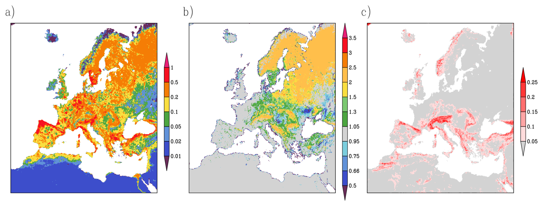
Figure 5 Surface roughness z0 [m] of GLOBE (a), ratio between z0 of MERIT and GLOBE (b), and deviations of subgrid slopes, where $\mathrm{0.1}\widehat{=}\mathrm{9}\mathit{°}$ (c). White colour is used for water grid points, where z0 is modulated by the wave height.

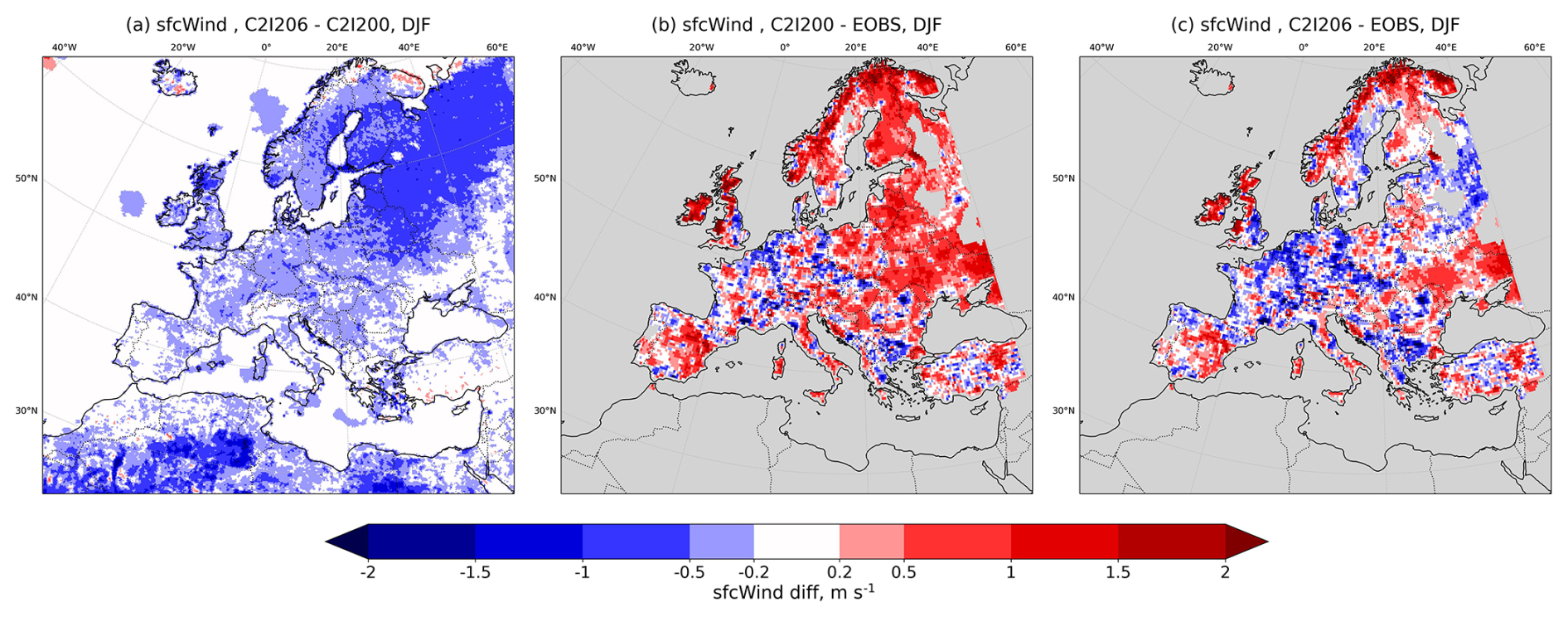
Figure 6 Sensitivity and Bias of ICON-CLM with respect to orography data from MERIT (test) and GLOBE (reference), and oro+tuning. Mean differences of sfcWind for DJF for 1980–1984 between test and reference (a) as defined in Table 6 in column “signal”, reference and E-OBS (b), and test and E-OBS (c).

Natural and anthropogenic transient Aerosol irad_aero (test: MACv2-SP*, reference: Tegen*)

For CMIP6-CORDEX, it is recommended (even mandatory for EURO-CORDEX, Katragkou et al., 2024) to use transient anthropogenic aerosols. Thus, as the reference experiment was set up with the standard Tegen aerosols used for NWP, which are constant in time (with a mean annual cycle), the impact of the transient aerosols prescribed by the MACv2-SP climatology was tested. The Tegen climatology is representative for the early to mid-90s, which is a period when anthropogenic emissions over Europe are already reduced compared to the 80s, for which the experiments were conducted. Thus, the transient MACv2-SP climatology contains realistically higher Aerosol optical depth (AOD) values for the 80s.

The sensitivity of the climatology for AOD and related meteorological quantities is largest in summer (Fig. 7). The respective sensitivity for winter is shown in Fig. S4. In summer, the differences in AOD (Fig. 7a) are strongly correlated with rsds differences (Fig. 7b). There is nearly no impact on clt (Fig. 7f). AOD is increased and shortwave radiation is reduced over Europe by approximately 10 W m⁻². Consistently, a cooling of tasmax by 0.5 K is found in Europe.

In northern Africa and the eastern Mediterranean, the AOD signal is highly correlated with rsds but neither with tasmin nor with tasmax (Fig. 7c and d). The latter are highly correlated with the downwelling longwave radiation rlds increase of 10 to 20 W m⁻² (Fig. 7e). Increased rlds can partly be explained by increased cloud cover at night. However, the cloud cover difference is small and cannot be detected below 500 hPa, so the effect on thermal radiation is minor. Kinne (2019b) clearly shows a warming due to direct radiative effects of the MACv2 aerosol over northern Africa and Arabia. The explanation is that the “mineral dust aerosol particles in those regions are relatively large, elevated (off the ground) and absorbing”. With that, mineral dust can “contribute to a significant greenhouse effect”. However, it is debatable if MACv2 overestimates the increase of longwave radiation as it neglects the natural variability of mineral dust both in terms of variability of particle sizes and mineralogical composition, which can have a considerable influence (e.g. Sicard et al., 2014; Gao et al., 2026, and the references therein).

In winter, the impact of AOD on rsds is much weaker in Europe than in summer. A weak cooling is found in southern and eastern Europe in tasmax and tasmin (Fig. S4).

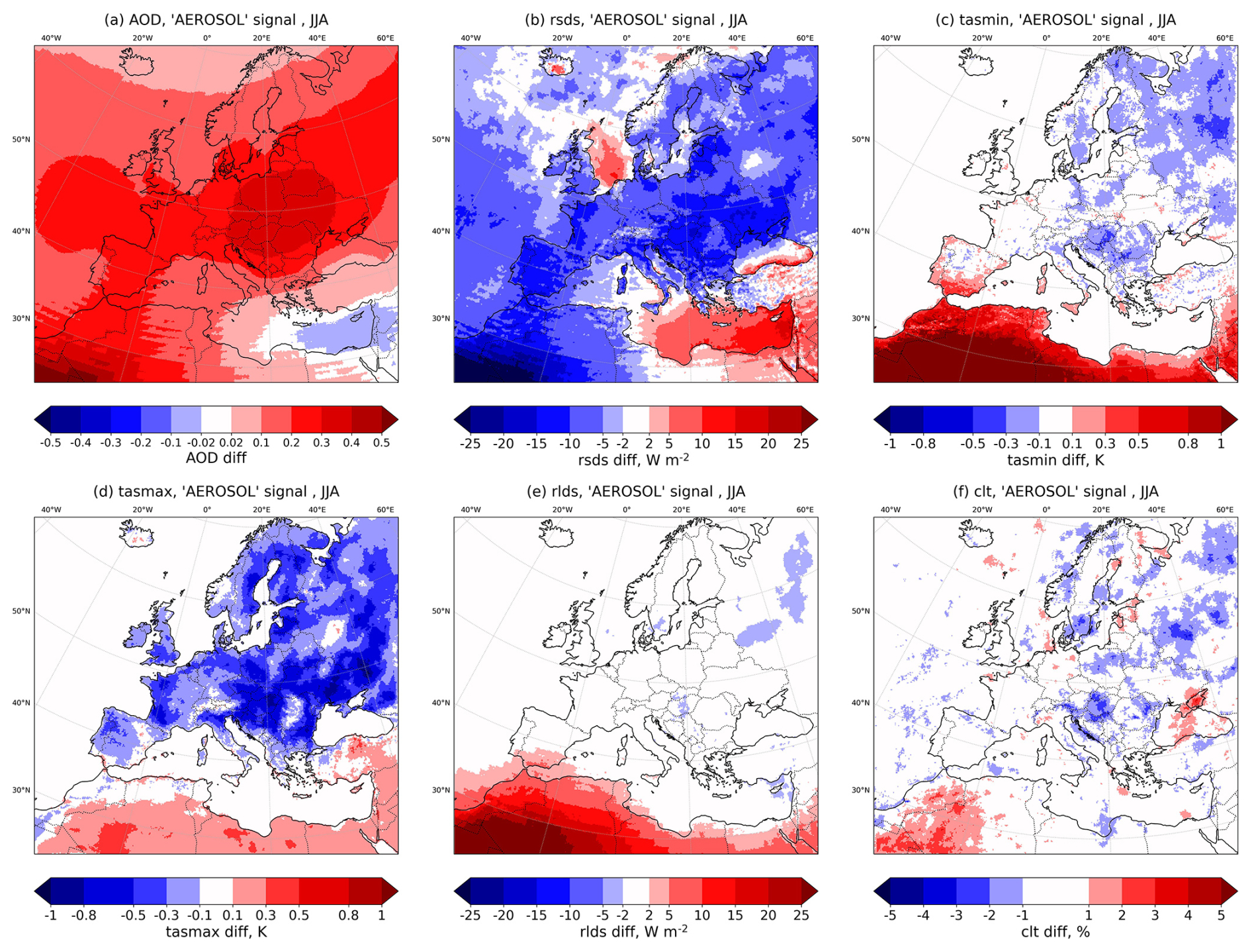
Figure 7 Mean differences (JJA 1980–1984) of Aerosol Optical Depth AOD (a), rsds (b), tasmin (c), tasmax (d), rlds (e) and clt (f) for the test with transient aerosol data (MACv2-SP, C2I105) minus the reference with Tegen aerosols (C2I101), cf. Table C1.

However, for the new treatment of the indirect aerosol effect (aerosol-cloud-fb, icpl_aero_gscp=3), we only found a mean sensitivity of (“Avg” sens: DJF = 0.8, JJA = 1.1). The values are similar for all variables. Thus, the impact is not significant.

3.2.2 Parameters of surface and subsurface processes

In this section, we discuss ICON-CLM sensitivities to parameter changes of surface and subsurface processes (see Tables 5 and 6). Those parameters that do not exhibit a signal-to-noise ratio (i.e., sensitivity) significantly higher than one are introduced only shortly hereafter, but the results of the tests are neither shown nor further discussed.

The change of the scaling factor of minimum resistance to plant transpiration rsmin_fac from 1.0 to 1.2 exhibits a mean sensitivity of (“Avg” sens: DJF = 0.7, JJA = 1.0).

We tested the increase of bare soil minimum resistance to turbulent fluxes cr_bsmin in (C2I111–C2I200) from 110 to 150 s m⁻¹. The results are similar to those found for rsmin_fac increase and exhibit a mean sensitivity of (“Avg” sens: DJF = 0.9, JJA = 1.1).

The factor rat_lam is scaling the resistance to turbulent latent heat flux over land in comparison with that over ocean surfaces. For the change from 1.0 to 0.8, we found a sensitivity for clt of (“clt” sens: DJF = 2.1, JJA = 2.2) and (“Avg” sens: DJF = 1.2, JJA = 1.5). Due to the definition of the signal as a linear combination of four simulations (see Table 6), the noise level is twice the noise level used for the definition of the sensitivity in Table 4. Considering the higher noise level of rat_lam test results, the results can be regarded as not significant.

itype_z0 (test:3, reference:2)

A change of the parameter value for itype_z0 from 2 to 3 results in an increase of surface roughness z0 in mountainous regions. For itype_z0=2, z0 is determined from land-cover-related roughness considering tile-specific land use class. For itype_z0=3, additionally, the subgrid-scale orography is considered. We found a mean sensitivity of (“Avg” sens: DJF = 3.0, JJA = 2.5) resulting from high sensitivities of mean sea level pressure psl and wind speed ws. The impact of the change on tas, pr_amount, and sfcWind is shown in Fig. 8. A systematic effect is found for the wind speed, which is reduced in mountainous regions. Additionally, the effects on psl and the turbulent fluxes hfls and hfss are shown in Fig. S5. The impact on psl is up to 0.3 hPa and thus negligible. In winter, the hfls is increased and hfss is decreased slightly in mountainous regions. In summer, the hfss is systematically decreased by up to 10 W m⁻² in mountainous regions in the Mediterranean while causing a decrease in tas by up to 0.5 K.

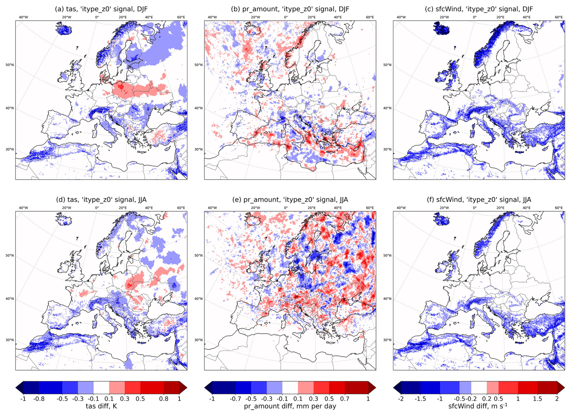
Figure 8 Mean differences (1980–1984) of tas (a, d), pr_amount (b, e), and sfcWind (c, f) in winter (DJF, top) and summer (JJA, bottom) for the type of roughness length data itype_z0.

rlam_heat (test: 6.25, reference: 10)

The parameter is the scaling factor of turbulent heat flux resistance at the surface (see also Table 1). For the change of the scaling factor of resistance to turbulent heat fluxes rlam_heat from 10 to 6.25, we found a sensitivity for hfls_o (“hfls_o” sens: DJF = 7.0, JJA = 5.7) and (“Avg” sens: DJF = 1.9, JJA = 1.6) on average. The decrease of rlam_heat leads to a strong increase of hfls_o over the Mediterranean Sea and the Atlantic Ocean in winter. In summer, the effect is reduced in the Atlantic but remains high in the Mediterranean Sea (Fig. 9 left).

The impact on tas, pr_amount, and rlds is shown in Fig. S6. We found an increase of tas over the entire domain by 0.3 K in winter and not in summer. This occurs, since the two effects of increased latent heat flux on the cloud cover, as later discussed in detail in Sect. 3.4.1, result in a winter increase of long wave downward radiation rlds due to an increase of low cloud cover. In summer, the reduction of short wave and increase in long wave are small and similar.

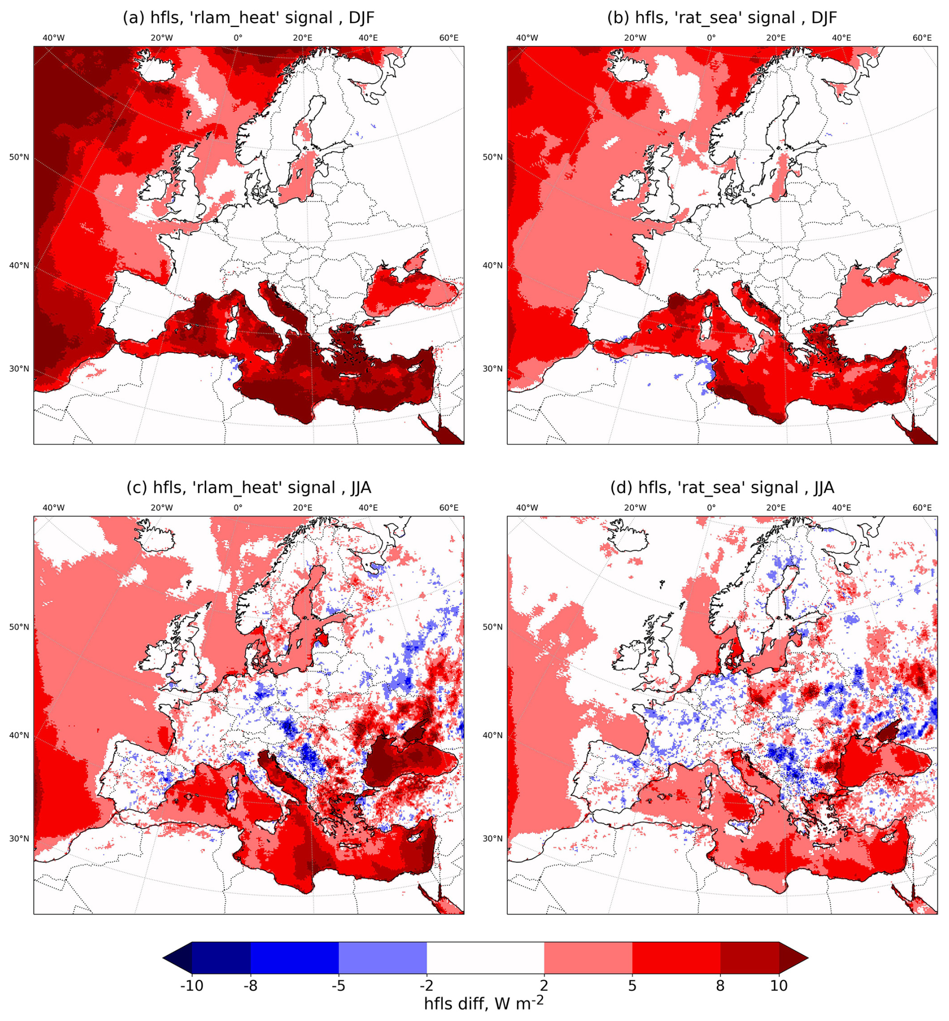
Figure 9 Mean differences (1980–1984) of hfls for reduced resistance to turbulent heat fluxes rlam_heat (left, a, c), reduced resistance to turbulent heat fluxes over water rat_sea (right, b, d), DJF (top), JJA (bottom).

rat_sea (test: 0.4, reference: 0.7)

The scaling factor of resistance to turbulent heat fluxes over the sea surface rat_sea is reducing the resistance over water in comparison with land surfaces. We found high sensitivities for hfls_o of (“hfls_o” sens: DJF = 4.5, JJA = 4.0) and (“Avg” sens: DJF = 1.4, JJA = 1.2) on average, which is similar to rlam_heat. Figure 9, right, shows the impact of increased resistance on hfls, which is spatially very similar distributed to the effect of reduced rlam_heat. The impact on tas, pr_amount and rlds is shown in Fig. S7 as for rlam_heat.

tune_albedo_wso(1) and tune_albedo_wso(2) (test: $\mathrm{0.1}/-\mathrm{0.1}$, reference: $\mathrm{0.0}/\mathrm{0.0}$)

The albedo correction, now as a modification of the official ICON release source code available (Sect. 2.2.2), for dry soils (𝚝𝚞𝚗𝚎_𝚊𝚕𝚋𝚎𝚍𝚘_𝚠𝚜𝚘(1)=0.1) is changing the albedo by up to 0.1 if the upper soil layer is dry. For tas we found a sensitivity of (“tas” sens: DJF = 3.5, JJA = 3.8) and of (“Avg” sens: DJF = 3.1, JJA = 2.6) on average. Figure 10 shows a decrease of tasmin, tasmax in summer of 0.5 to 1.5 K in the Mediterranean due to an increase of short wave outgoing radiation flux at the surface rsus of 10 to 20 W m⁻². Additionally, Fig. S8 shows a slight decrease of pr_amount and hfls in JJA in central to northern Europe due to increased rsus, which is an indirect effect.

The albedo correction for wet soils ($\mathtt{\text{tune\_albedo\_wso(2)}}=-\mathrm{0.1}$) is changing the albedo by up to −0.1 if the upper soil layer is wet. It exhibits a very weakly significant impact on the reflected solar radiation in the southern part of the domain in summer and no significant impact on the other surface energy budget components, nor on tas.

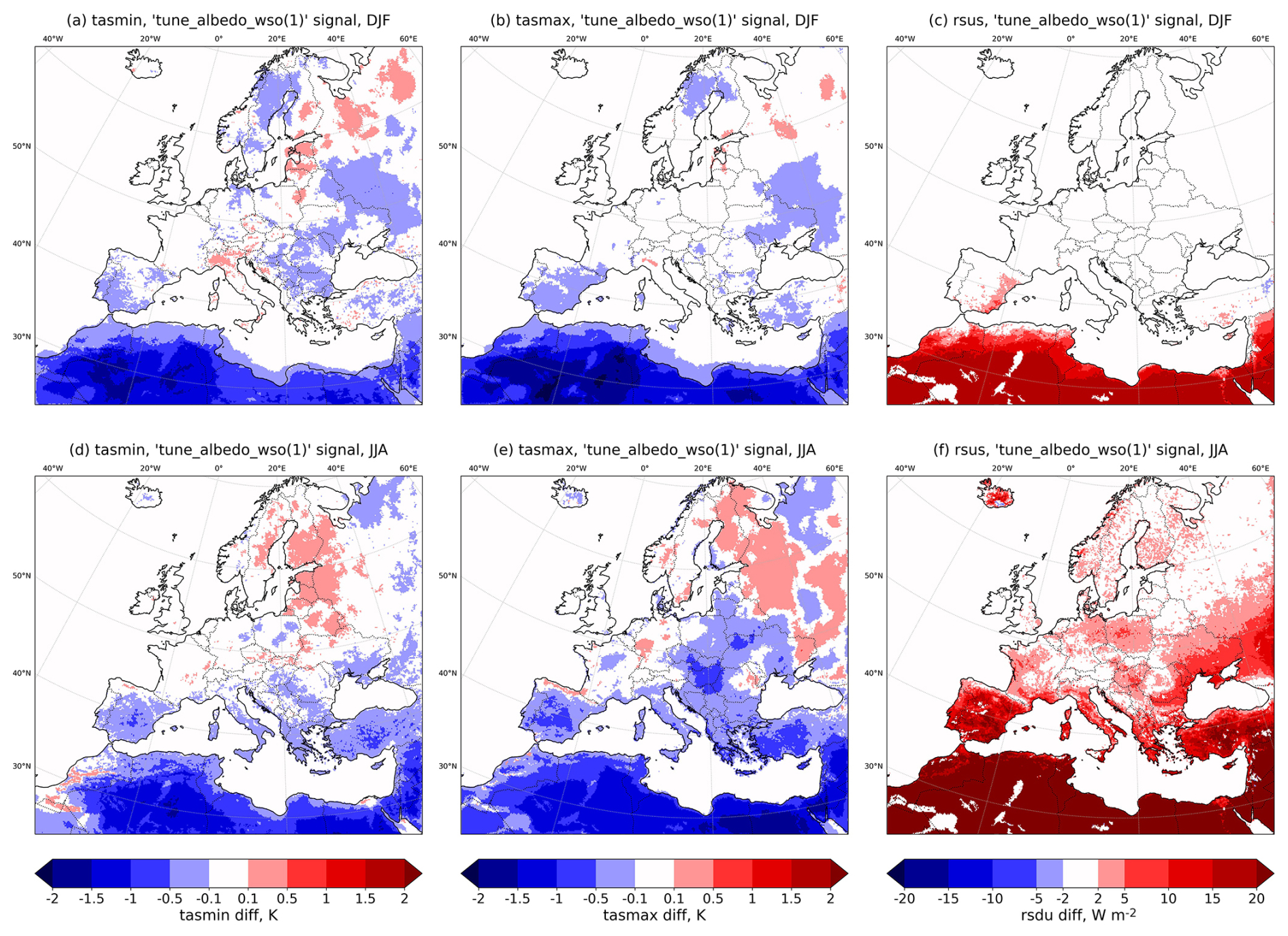
Figure 10 As Fig. 8 but for tasmin, tasmax and rsus and increased albedo for dry soils near surface tune_albedo_wso(1).

itype_hydmod (test: 1, reference: 0)

The new parameterisation of horizontal transport of subsurface water due to gravitation itype_hydmod=1 shows high sensitivities for summer tasmax (“tasmax” sens: DJF = 1.3, JJA = 5.3), for latent heat flux over land hfls_l and (“hfls_l” sens: DJF = 2.3, JJA = 3.7) and (“Avg” sens: DJF = 1.2, JJA = 2.7) on average. The impact on tas, pr_amount and hfls is shown in Fig. S9. It exhibits a warming over mountains and a cooling in water down-flow regions due to a decrease/increase in hfls, e.g., in the Alpine region and the Po valley, respectively, and in particular in the dry summer season. This is consistent with the physical expectation as the lateral redistribution of water results in a changed evaporative fraction affected by surface and subsurface heterogeneities and orography.

In northern Africa, there is an increase of hfls of 3 to 5 W m⁻². We hypothesise that this is due to the reduced vertical gravitation flux in this parameterisation.

Unfortunately, this parameterisation was not included in the officially released model version used for configuration optimisation in this study, so it was not considered further.

3.2.3 Parameters of planetary boundary layer, mixing, and convection-related processes

DT_PHY (test: dt2*, reference: dt1*)

The frequency of calling of the convection, radiation, subgrid-scale orography drag, and gravity wave drag parameterisations might have a systematic impact on the simulation results if the time increment DT is too large. However, the computing time is increasing with decreasing DT. This test investigated the opportunity of larger DT values. The sensitivity found for DT_PHY is for sfcWind (“ws” sens: DJF = 27, JJA = 8.3) and (“Avg” sens: DJF = 5.1, JJA = 1.9) on average. The dependency of the solution on the time step (see Fig. S10) indicates the need for the shorter time step. Consistently herewith, the analysis of the results showed that the longer time step corrupts the development of gravity waves, so the larger DT is not used.

tkhmin and tkmmin (test: $\mathrm{0.3}/\mathrm{0.375}$, reference: $\mathrm{0.6}/\mathrm{0.75}$)

For the change of minimum turbulent transport coefficients for heat and momentum tkhmin,tkmmin we found a sensitivity for tasmin of (“tasmin” sens: DJF = 2.2, JJA = 2.3) and (“Avg” sens: DJF = 1.5, JJA = 1.3) on average. Reducing the minimum vertical transport reduces the mixing in a stable atmosphere. Stable conditions occur particularly in winter and at night. This reduces the sensible heat flux at the surface, thereby increasing cooling during the night. In cloudy conditions, it helps to dissolve the low cloud cover, which exists over too long time spans otherwise.

Figure S11 shows the impact of the reduction of the parameter values on tasmin, hfss, and clt. We find a reduction to tasmin by 1 K in winter and 0.5 in summer, and no significant impact on precipitation. In winter, the downward positive sensible heat flux hfss is reduced by 2 W m⁻² in stable stratification, in particular in snow-covered regions and in the desert. In summer, this effect is weaker. The cloud cover and the longwave downward radiation are slightly increased, but do not have a dominant impact on the near-surface temperature. However, the overall effect decreases the simulation quality, and thus, these parameter value changes have not been considered in the new reference, and they are not used as optimisation parameters.

lstoch_sde (test: 1, reference: 0)

The stochastic shallow convection scheme (lstoch_sde=.true.) aims at parameterising the shallow convection in simulations resolving deep convection, i.e., at horizontal grid sizes smaller than 20 km. It has to be used together with setting both lrestune_off and lmflimiter_off to “True”. The parameter sensitivity for pr_amount of (“pr_amount” sens: DJF = 3.8, JJA = 2.0), for hfls_l of (“hfls_l” sens: DJF = 3.1, JJA = 2.6) and (“Avg” sens: DJF = 2.1, JJA = 2.0) on average.

Figure 11 shows the impact on tas, pr_amount, and rsds. The pr_amount in winter is strongly decreased due to flow disturbances at the inflow boundary, at coastlines, and at some of the mountain chains, in particular when the wind speeds are high. The precipitation is increased inland, indicating a potentially strong relation to sea breeze circulations. In summer, mainly the mountainous pr_amount is increased by enhanced shallow convection. Herewith, rsds is consistently reduced by 5 to 10 W m⁻² over large parts of the domain in summer.

An unexpected effect is the reduction in tas in the north-east of the domain. A more detailed inspection revealed a reduction of rlds due to increased mixing.

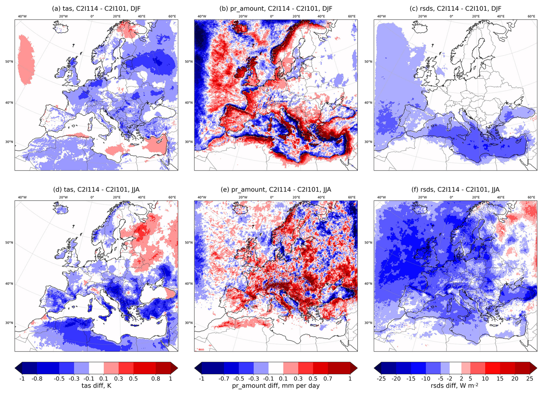
Figure 11 As Fig. 8 but for tas, pr_amount, and rsds and for the application of the stochastic shallow convection scheme (lstoch_sde=.true.).

3.2.4 Parameters of microphysics and cloud cover diagnostic

The parameterisations of precipitation and cloud cover diagnostics described in Sect. 2.2.1 have a direct impact on the irradiance at the surface rsds and rlds. The most important ICON parameters are considered in this study.

Grid Scale Precipitation (GSCP) (test: 2-ice*, reference: 1-ice*)

The 1-moment scheme (mass; inwp_gscp=1) with two categories of ice (cloud ice, snow) is tested with new ice nucleation (inwp_gscp=3). We tested it together with recommended configuration settings (see C2I108 in Table C1). Overall, we found high sensitivity on inwp_gscp change (“Avg” sens: DJF = 4.0, JJA = 6.0) and especially high values for rsds (“rsds” sens: DJF = 9.7, JJA = 10.2).

As shown in Fig. S12, the new ice nucleation generates much higher pr_amount at the eastern outflow boundary and in mountainous regions in summer. The strong increase in rsds values in winter in the Mediterranean (up to 15 W m⁻²) and over the North Atlantic and northern Europe (up to 40 W m⁻²) in winter leads to an increase in tas of up to 0.8 K in winter and 1 K in summer in the corresponding regions. Additionally, we found a distinct reduction of tas in the north-eastern part of the domain in winter, where the pr_amount is not systematically influenced. This indicates an increase in cloud base height, resulting in reduced rlds. Due to the reduction of the overall simulation quality, the scheme tested is not used in the new 12 km grid reference (see also Fig. 15).

inwp_cldcover (test: 1, reference: 3)

The subgrid-scale cloud cover scheme is a parameterisation of the cloud cover due to vertical mixing processes (convection, turbulence) if the rh is below 100 %. Here, the impact of the scheme, already available in the COSMO model (inwp_cldcover=3), is investigated in comparison with the reference (inwp_cldcover=1) cloud cover diagnostics. The latter is used in the radiation scheme and has no direct impact on precipitation. We found a sensitivity for clt of (“clt” sens: DJF = 6.9, JJA = 6.1) and (“Avg” sens: DJF = 2.2, JJA = 2.6) on average.

The impact on tas, rsds, and rlds is shown in Fig. 12. We found a rsds change of −3 and −5 W m⁻² in winter and summer, respectively, due to increased cloud cover, together with an rlds increase of up to 10 and 6 W m⁻² in winter and summer, respectively. This resulted in an increase in radiative forcing and an increase in tas over North Europe by up to 1 K in winter and over land in summer by approximately 0.3 K.

Figure 12 As Fig. 8 but for inwp_cldcover=3 and for tas (a, d), rsds (b, e), and rlds (c, f).

The results in radiation components show an increase in clt and a reduction of the cloud bottom height, in particular in winter, and the relevance of the diagnostic cloud cover for tuning of the surface forcing.

The process-specific subgrid-scale cloud cover diagnostics and their tuning parameters (allow_overcast, tune_box_liq, tune_box_liq_asy and others, see Sect. 2.2.1), were introduced for the new scheme in ICON (inwp_cldcover=1); they are not available for the old scheme from the COSMO model (inwp_cldcover=3). This study, therefore, uses the latest tuning options of the new subgrid-scale cloud cover scheme.

allow_overcast (test: 0.9, reference: 1.0)

The shape factor allow_overcast of the quadratic dependence of subgrid-scale cloud cover on rh is a parameter of the cloud cover scheme itype_cldcover=1. We found a sensitivity for clt of (“clt” sens: DJF = 3.3, JJA = 4.0) and (“Avg” sens: DJF = 1.7, JJA = 2.6) on average.

As mentioned in Sect. 2.2.3, smaller values of allow_overcast result in higher subgrid-scale cloud cover. Figure 13 shows the sensitivity of reducing allow_overcast from 1.0 to 0.9.

Figure 13c and f show an increase of total cloud cover, in particular in summer and over the sea, where the cloudiness is mainly partial. During winter, a decrease in rsds (Fig. S13) is found over land in central and southern Europe, and an increase of 3 W m⁻² in downward longwave radiation over northern and central Europe, which results in an increase of up to 0.5 K in tas in snow-covered regions.

While over the Mediterranean and southern Europe, the radiative forcing effect is close to zero, over northern Europe, the daily mean tas (Fig. 13) is increased by up to 0.5 K and tasmin by up to 1 K. During winter, the sunshine duration is short in northern Europe. Consequently, the prevailing effect is an increase in the long-wave radiation absorbed by the surface (see Fig. S13).

The increase in clt can be explained by frequent cyclonic synoptic situations leading to overcast (total cloud cover of 1). In these situations, a reduction of allow_overcast can lead to an increase of clt at additional model levels, in particular for low clouds, reducing the bottom cloud height and making the existing cloudy layer optically more opaque. However, it can not lead to an increase in the clt greater than 1. This argument may explain the low sensitivity of the clt to the change in allow_overcast in northern Europe in winter, an increase of rlds, and a strong increase of tas, in particular in snow-covered regions.

Figure 13 shows that the increase in clt in summer is much higher than in winter, resulting in a rsds reduction of 20 W m⁻² in summer and of 10 W m⁻² in winter and over the entire northern part of the domain and in relatively small changes in rlds (see Fig. S13). Figure 13d consistently shows a reduction in tas of about 0.3 to 0.5 K in particular during the day. This is shown by the reduction of tasmax of up to 1 K.

An inflow boundary effect can be found in pr_amount in winter and summer (Fig. 13b and e). Since the cloud cover diagnostics are not used in the microphysics scheme, this effect is probably caused by a feedback of reduced reflected shortwave radiation on precipitable water.

Figure 13 As Fig. 8 but for reduced allow_overcast and tas (a, d, left), pr_amount (b, e, center) and clt (c, f, right).

tune_box_liq (test: 0.07, reference: 0.05)

The increase of the range of relative humidity tune_box_liq around 100 % from 0.05 to 0.07, within which the cloud cover is increasing from 0 to 1 (see Eq. 2), exhibits the highest sensitivity for clt (DJF = 2.1, JJA = 2.6). The mean sensitivities “Avg” are (DJF = 1.2, JJA = 1.7). This increases the subgrid-scale cloud cover and reduces rsds.

The effect of increasing tune_box_liq is very similar to that of reducing allow_overcast to 0.9 but weaker, in particular in summer. While the effect of reducing allow_overcast is reflected in the appearance of full overcast areas, strongly influencing insolation, the effect of increasing tune_box_liq is reflected in a slight increase of partial cloudiness areas (see Figs. 14c and 13f) with a weaker effect on insolation and thus on tas (see Figs. 14a and Fig. 13d). For comparison, Fig. S14 shows tasmax, rsds and rlds in winter and summer.

Figure 14 As Fig. 13 but for reduced tune_box_liq (top) and increased tune_box_liq_asy (bottom) and JJA only.

tune_box_liq_asy (test: 4.0, reference: 3.25)

For the scaling factor determining the asymmetry term of the cloud cover for over- and undersaturation tune_box_liq_asy, we found a sensitivity for clt of (“clt” sens: DJF = 3.5, JJA = 4.3) and (“Avg” sens: DJF = 1.5, JJA = 2.3) on average.

The effect of increasing tune_box_liq_asy is very similar to that of reducing allow_overcast and increasing tune_box_liq. There is an increase in clt (see Fig. 14) and a reduction of rsds (see Fig. S15, center). As expected (see Sect. 2.2.3), the effect of increasing tune_box_liq_asy is stronger than the effect of increasing tune_box_liq, leading to a larger increase of partial cloudiness. The comparison of the results shown in Figs. 13, S13, 14, and S15 show that the effects of decreasing allow_overcast and increasing tune_box_liq_asy are of similar magnitude in tas, rsds and rlds. However, the spatial structures are different and accumulate to significantly different patterns in tas, tasmax and tasmin.

3.3 New reference configurations, their quality and the inferred tuning aim

The original reference configuration (C2I101) has been further developed based on a series of test simulations of parameter settings used in climate mode of the COSMO model, of new external parameters, and of the ICON model developments described in Sect. 3.2. The new expert decision based reference configuration is used in the C2I200 and C2I200c simulations and is given in Table D1.

Figure 15 summarises the evaluation results for each parameter tested (see Table 5) in terms of the index ScoPi for the PRUDENCE regions (RCM tuning strategy stage 2, step 2d). It shows that, in particular, the parameter change of AEROSOL-SP (C2I105), of parameter lstoch_sde (C2I114) and of inwp_cldcover (C2I117) improve the model quality.

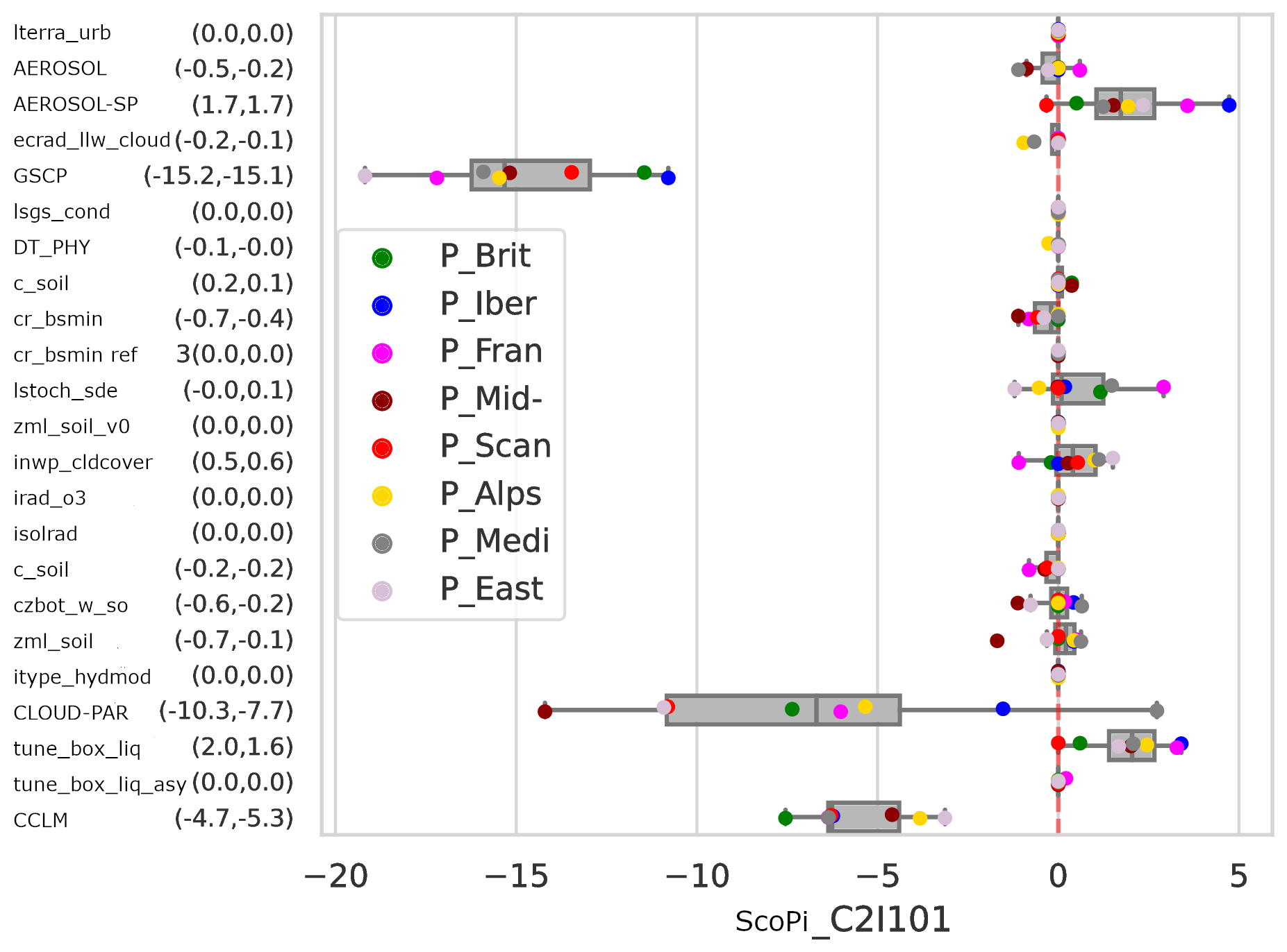
Figure 15 ScoPi_region based on the differences in the mean BIAS of all variables in Table 2 between the observations and each simulation of Table C1, against the ones of the reference simulation C2I101. The colours indicate the eight PRUDENCE analysis regions. The numbers given on the y-axis labels in brackets are the ScoPi_simulation. The values represent the averages over all eight PRUDENCE regions, weighted by the distance to Mid-Europe, one of the main areas of interest (first value), and by their area (second value), respectively (see Table 3). Higher ScoPi values mean that the test simulation is more consistent with the selected observations than the reference simulation.

The expert decision to use a test parameter value in the new reference is based on scientific arguments (Fig. 12g). Here is a breakdown of some decisions for the new intermediate reference configuration C2I200, as a basis for further tuning: The urban parameterisation (lterra_urb) is not used since the evaluation data used do not consider the urban effect. The new aerosol climatology MACv2-SP is used since it exhibits highly positive ScoPi, and the quality of the data has been shown independently to be higher than for the Tegen aerosol data. The parameterisation of long-wave radiation scattering by clouds (ecrad_llw_cloud_scat) shows no impact on the results and is not used. The enhanced precipitation scheme by two ice phases is not used since it increases the computing time by 30 % and shows highly negative ScoPi. A higher depth of hydrologically active soil (czbot_w_so) is used since it is well tested in climate mode in the COSMO model, preventing extremely low summer latent heat flux, and shows neutral ScoPi results. The subgrid-scale condensational heating in the atmosphere due to the non-convective part of diagnosed cloud water (lsgs_cond) is not used since the sensitivity is low. Lower frequency of execution of convection, radiation, SSO, and gravity wave drag parameterisation is rejected since it negatively affects some results significantly. The stochastic differential equation for subgrid scale cloud cover (lstoch_sde) is not used since it does not result in a positive ScoPi score. The COSMO sub-grid scale cloud scheme does not show significant improvements (inwp_cldcover) and is not used. The same applies to the consideration of subgrid scale orography in the roughness length (itype_z0). The distribution of soil layers (zml_soil) using 10 instead of 8 soil layers is used since it is well tested in the climate mode with the COSMO model and does not show a negative impact on the ICON results. The parameterisation of horizontal subsurface water fluxes (itype_hydmod) shows a significant impact on tas in a physically reasonable way, but it is not used since the parameterisation is not available in the released ICON model version. The new cloud cover diagnostics parameters exhibit negative ScoPi and are not used in the new reference. They are tuned independently by expert analysis and LiMMo tuning. These scientific arguments are resulting in a new reference configuration evaluated as C2I200c.

In addition to the parameters considered in C2I200c, further new external parameters have been investigated and considered in the second new reference configuration C2I250c introduced by expert decision: The HWSD v2.0 soil data have a higher spatial resolution than the previously used FAO data and are regarded as having a higher quality over Europe. They are less sandy, and using them reduces the summer cold bias. The usage of MODIS cloud condensation nuclei number allows the consideration of the aerosol-cloud feedback in the ICON model. The higher-resolution MERIT orography increases the surface roughness in North-East Europe. Together with the corresponding parameter tuning, it reduces the positive wind speed bias in this region.

In the following, we discuss the quality of the evaluation simulation C2I200c and define a model tuning aim addressed by expert and LiMMo tuning. The quality problems found in the evaluation simulation C2I250c are similar, and they are not shown additionally.

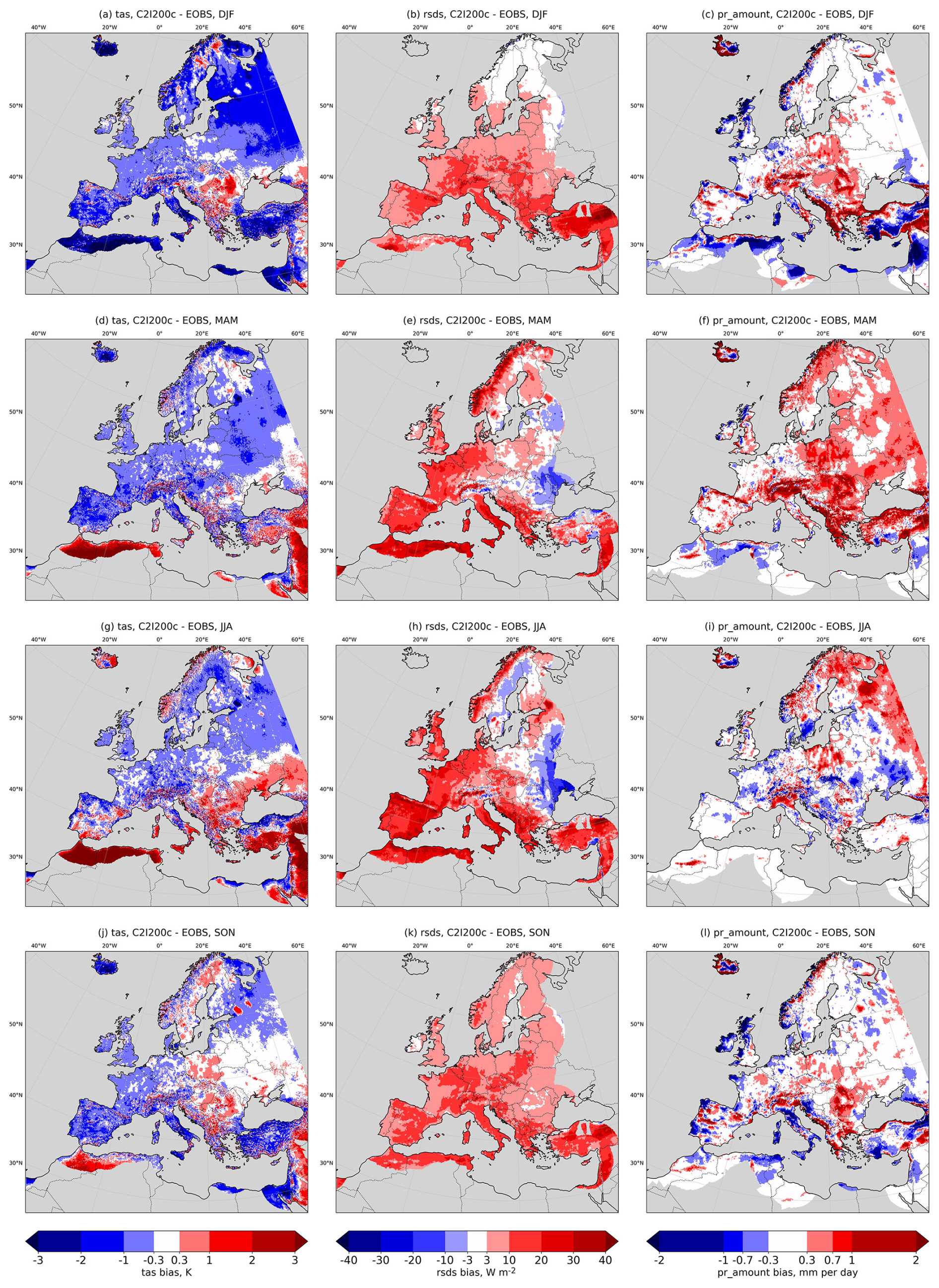
Figure 16 Mean seasonal biases (2003–2008) of tas (left), rsds (centre), pr_amount (right) for revised reference configuration C2I200c compared to E-OBS data for DJF (top), MAM (2nd row), JJA (3rd row), and SON (bottom).

Figure 16 shows the quality of the reference simulation C2I200c. From winter to summer, we found a pronounced negative bias for tas and a positive one for rsds, which are contradictory signals, and this complicates the expert tuning. The precipitation biases are small, except for spring, where dry biases dominate the eastern half of the domain and for some coastal regions, where wet biases are found. Figure 17 shows a detailed analysis of pr_amount in comparison with station observations for Germany and Poland. The annual cycle (Fig. 17a) exhibits an overestimation of around 10 % and 15 %, respectively, for most of the months. The mean diurnal cycle (Fig. 17c) shows a strong overestimation of the late night to noon precipitation and a too early precipitation maximum. In Germany, the morning minimum is not simulated at all. The histogram shown in Fig. 17d shows an overestimation of low (< 2 mm h⁻¹) and underestimation of high to extreme events. The annual cycle of rsds in Germany and Poland confirms the positive bias already found in the comparison with E-OBS data (Fig. 17b).

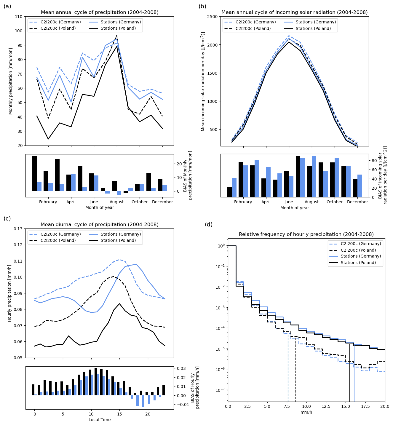
Figure 17 Annual cycle of pr_amount and rsds (2004–2008) for C2I200c in comparison to station data in Germany and Poland station data (top), diurnal cycle of pr_amount (bottom, left), and relative frequency distribution of hourly precipitation (bottom, right). Vertical lines denote the 99.99th percentile. The number of stations for rsds is 23 for Poland and 34 for Germany; for pr_amount it is 54 for Poland and 1009 for Germany.

The comparison of latent heat flux over the ocean hfls_o with satellite data set HOAPS in DJF and JJA (Fig. S20) shows a strong overestimation almost everywhere in all seasons. The only exception is the eastern Mediterranean in summer, where an underestimation was found.

The results reveal that tas is underestimated even though the forcing, represented by rsds, is overestimated. Addressing these biases is regarded as a challenging and relevant first aim of tuning the 12 km configuration in the EURO-CORDEX domain.

Furthermore, the results exhibit an overestimation of the latent heat flux over water, an overestimation of coastal precipitation, in particular at inflow positions, and a nearly correct amount of seasonal precipitation over most continental regions. Reducing the overestimation of hfls_o without increasing the seasonal precipitation bias is identified as a second tuning aim. A further improvement of the diurnal cycle and extreme precipitation is regarded as hardly possible at 12 km model grid resolution.

3.4 Parameter tuning

In Sect. 3.2, the simulation results for the external and the main tested model parameters have been discussed. In Sect. 3.3, the change of 15 parameter values in the reference configuration has been discussed, and six have been updated to be used in the new reference.

In this section, we present the results of the tuning of the remaining 12 parameters given in Table 6. We apply the commonly used method of expert tuning and, for the first time in a real climate case study, the LiMMo tuning method (Petrov et al., 2025).

3.4.1 Expert tuning

The task of expert tuning is to find an optimised model configuration based on the test simulation results for the tuning parameters and values given in Table 6. The procedure applied was as follows. Each expert was invited to suggest an Expert configuration. After discussion of all Expert configurations based on a comparison of the model bias, parameter sensitivities and configuration changes suggested, ten of the Expert configurations have been simulated and evaluated using the test simulation and evaluation procedure. The configurations C2I266c to C2I272c given in Table 7 are five of these configurations. New Expert configurations were suggested, aiming at further optimising the best configuration found, which was C2I268c. The configurations C2I277c to C2I280c are four of the final configurations simulated and evaluated. However, the improvements found have not been significant, so that C2I268c was identified as the optimised Expert configuration. It yielded the highest ScoPi values in comparison with the reference C2I200c and did not include any extreme namelist parameter values.

The configuration of C2I268c is using a combination of three test simulations for individual parameters: allow_overcast=0.9 (see Figs. 13 and S13), rlam_heat=6.25 (see Fig. S6), tune_albedo_wso$=(\mathrm{0.1},-\mathrm{0.1})$ (see Fig. S8). Reducing allow_overcast directly increases the low cloud cover and thus decreases the rsds in winter in mid to southern Europe by 3 W m⁻² (in winter the cloud cover is already high) and in summer in northern to mid Europe by 12 W m⁻². It increases the incoming long wave radiation as well, in particular in northern Europe in winter by 5 W m⁻², resulting in a warming in northern to mid Europe in DJF by 0.3 K. In summer, the increase of cloud cover and the resulting reduction of rsds is dominating the reduction in tas. This is combined with the heat flux resistance parameter rlam_heat reduction by 30 %. The latter increases hfls and hfss over water in winter and summer (see Fig. 9a and c for hfls). The dominating effect is an increased low cloud cover and the associated increase of incoming long wave radiation and tas in the entire domain in winter (Fig. S6c and a). In summer, the change in rsds and tas is close to zero. These two parameter changes reduce rsds and increase tas in winter in northern Europe. The third important change is that of the albedo. The dry soil albedo increase is decreasing the absorption of rsds in the Mediterranean, in particular in summer, resulting in a summer cooling. The wet soil albedo decrease has no significant impact on the results.

Table 7 Expert Configurations. Rows – tuning parameters (see Table 6), columns – the simulation IDs without “C2I” prefix (see Table D1). The “best” optimised Expert configuration C2I268c is emphasised with bold. The settings marked with “*” are given in Table A2. The missing values are equal to the corresponding values in the reference simulation C2I250c.

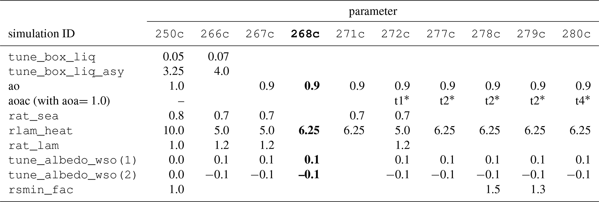
An intercomparison of the Expert configurations given in Table 7 shows that most of the configurations C2I266c to C2I272c are using albedo tuning for dry/wet soils. The result of C2I271c was the only one not showing a clear reduction of the summer warm bias in northern Africa and the eastern Mediterranean. This justified the albedo tuning. The configuration C2I266c is the only one using tune_box_liq and tune_box_liq_asy instead of allow_overcast together with different values for other parameters than in C2I268c. These values for other parameters together with allow_overcast=0.9 can be found in C2I267c and C2I272c.

The main differences between C2I272c and C2I268c are the values for rlam_heat=5 instead of 6.25 and rat_sea=0.7 instead of 0.8. An inspection of the evaluation results for C2I268c (see Figs. S16 and S19) and C2I272c reveals very similar summer and winter tas and winter rsds biases. The rsds summer values are slightly higher in C2I272c.

The evaluation of C2I266c and C2I272c (Fig. 18) indicates a slightly smaller bias in winter rsds in C2I266c. In summer, the biases for the Iberian Peninsula and northern Africa are similar. In C2I266c, a strong decrease of rsds is found in the central to eastern part of the domain. This indicates that the increase of tune_box_liq and tune_box_liq_asy by 40 % and 25 %, respectively, is generating too high cloud cover in some subregions of the domain.

The results of C2I266c to C2I272c lead to the selection of C2I268c as the new reference for further expert tuning. The configurations C2I277c to C2I280c comprise different annual cycles (aoac[m]) added to the allow_overcast mean value, as well as scaling factors for latent heat flux over land rat_lam and/or for minimum plant transpiration resistance rsmin_fac. These are used to further reduce the cold bias in tasmax (see Fig. S18), the positive bias of rsds in winter and the complex positive/negative bias in summer (see Fig. S19). However, the small improvements achieved did not justify using questionable parameter settings like the annual cycle aoac or strong deviations from parameter values used in operational NWP (rsmin_fac=1.5, rat_lam=1.2).

A final evaluation of additional model variables for the Expert configurations revealed a strong overestimation of the latent heat flux over water by C2I268c and by the other Expert configurations in comparison with the reference C2I200c (see Fig. 22).

The discussion demonstrates typical potential and drawbacks of expert tuning. On the one hand, it enables a definition of a new configuration by the combination of a small number of test simulation results and a small number of model variables very efficiently. On the other hand, two important drawbacks can be highlighted. First, model variables, which are not in the focus of interest, are typically neglected. Second, optimal parameter values cannot be determined, they can only be estimated. To find the optimal values, many more simulations would be necessary to consider cross-dependencies of parameterisations.

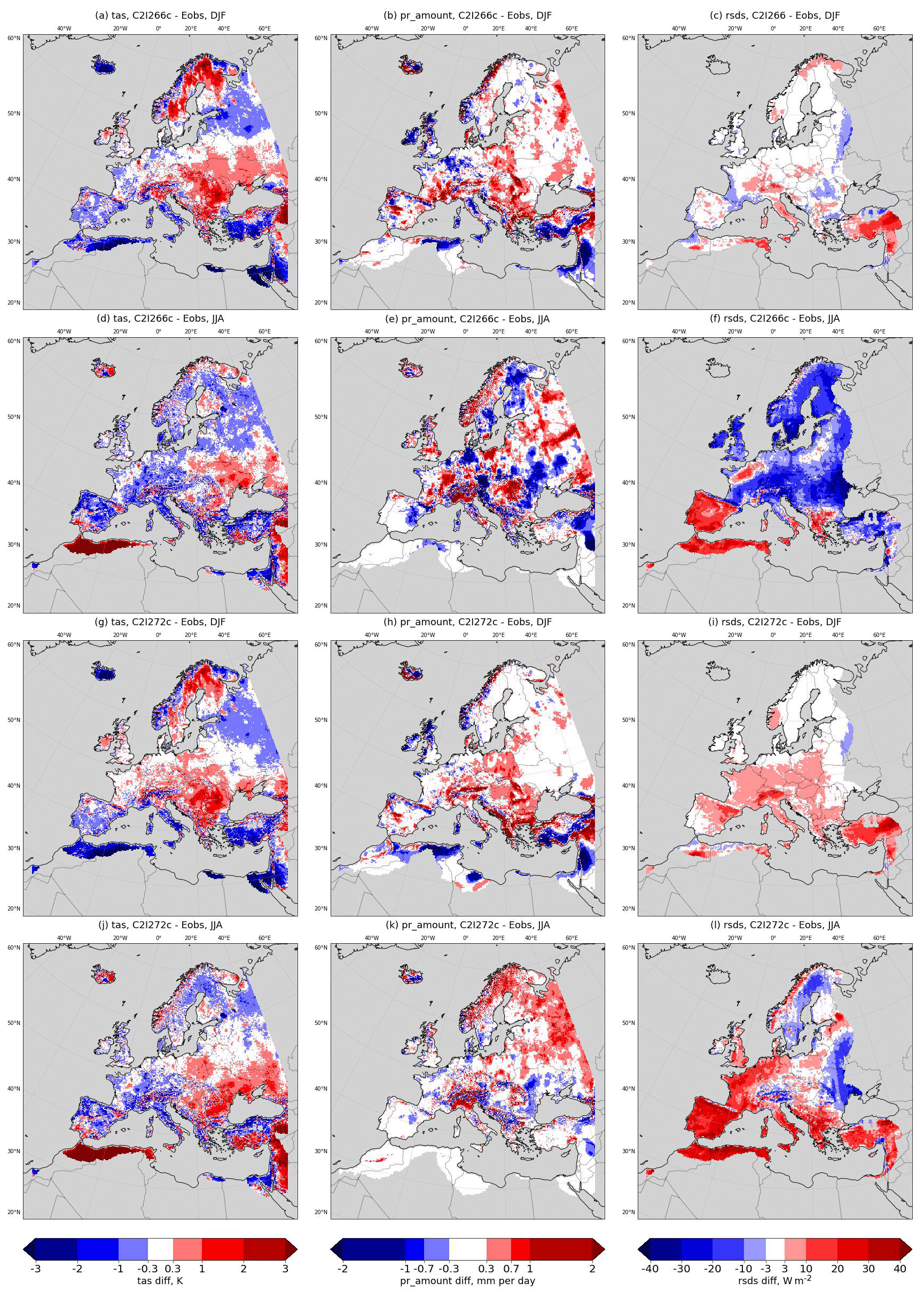
Figure 18 Expert tuning results: Seasonal mean differences in tas, pr_amount, and rsds for winter (DJF) and summer (JJA) for the simulations C2I266 and C2I272 to E-OBS.

3.4.2 LiMMo tuning

This section provides the settings used to configure the LiMMo framework. For detailed information on the LiMMo method, please refer to Sect. 2.4.

We selected the following list of parameters for the LiMMo tuning (check Table 6 to see the description of parameters): allow_overcast parameters ao and aoa, tune_albedo_wso(1), tune_albedo_wso(2), rlam_heat, rat_sea, rat_lam, rsmin_fac, tune_box_liq, and tune_box_liq_asy. Most of these parameters show high sensitivity (see Fig. 2), while tune_albedo_wso(2) signal is very weak. We decided to keep the latter under consideration for consistency, although we do not expect it to significantly affect the results.

As reference simulation, which defines the shift tensor of regression approximation (see Eq. 4), we used C2I250c (see Table D1), since it provides acceptable quality while incorporating the most up-to-date external data sets that we would like to use in the end. Moreover, C2I250c is the simulation of the revised reference configuration (see Sect. 3.3 and compare Fig. 12g).

To define the error norm that is minimised by the gradient method, we have tested two sets of weights for the model quantities, presented in Table 8. These weights are applied to define the quality measure of the configuration (error norm), given in Eq. (8), and have the unit sum. The main difference between the two sets of weights is the reduced weight of hfls_o in the second case. The residual 0.05 was added to rsds. As we will demonstrate later, this seemingly small adjustment has a strong impact on the LiMMo optimised configuration obtained.

Table 8 Weights of the model variables in the LiMMo optimisation. The columns are named after the model quantities (see Table 2).

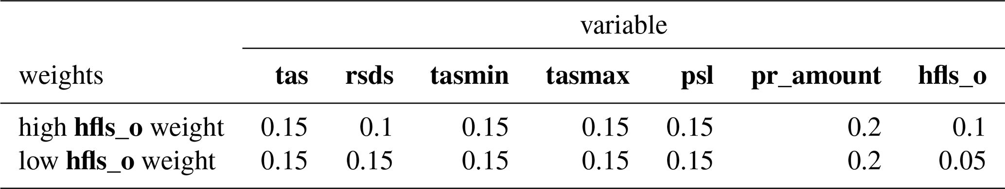
As mentioned in Sect. 2.4, the optimisation process (gradient descent) is restricted to the parameter space limited by MIN and MAX boundaries for each parameter. These values, along with the initial guess, are listed in Table 9. These values were chosen after extensive consultations with ICON developers and experienced users, to ensure the physical consistency of the optimised parameter values. In Table 9, we also present the resulting values for the two sets of weights from Table 8.

Table 9 Limit, initial, and optimal values of the model parameters in the LiMMo optimisation. MIN – minimal parameter values, INI – initial parameter values in optimisation, MAX – maximal parameter values. Also, the resulting values of optimisation for “high hfls_o weight” (simulated as C2I291c) and “low hfls_o weight” (simulated as C2I294c) from Table 8 are presented in corresponding columns. The settings marked with “^*” are given in Table A2.

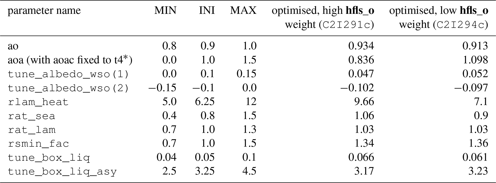
3.5 Optimised model configuration assessment

In this section, we assess the results of simulations using optimised ICON-CLM configurations by comparison with observations for key model quantities, with special emphasis on the tuning aim (reduction of tas cold bias and overestimation of rsds). The simulation quality for optimised configurations is shown in comparison with the reference simulation C2I200c. The optimised configurations investigated are the new reference configuration C2I250c obtained by expert judgement, the configuration (C2I268c) obtained by expert tuning and two LiMMo optimised configurations. C2I291c is obtained using a high weight for latent heat flux over water hfls_o and configuration C2I294c is obtained using a low weight of hfls_o (Table 8 in the error norm (Eq. 8)). Since the optimised configurations are based on the setup of C2I250c, a comparison between C2I268c, C2I291c, and C2I294c against C2I250c shows the impact of parameter tuning.

The presentation of the results is grouped into sections, corresponding to the main measures of model quality in this study: the ScoPi scores (Sect. 3.5.1), the seasonal Root Mean Square Error (Sect. 3.5.2), and the 2D seasonal BIAS plots (Sect. 3.5.3). Finally, we select the best configuration that we suggest to all users of ICON-CLM and for the production of EURO-CORDEX regional climate projections in Sect. 3.6.

3.5.1 ScoPi analysis

In Fig. 19 we present the ScoPi scores for the revised reference simulation (C2I250c), the simulation (C2I268c) using the expert tuning, and the simulations C2I291c and C2I294c) using the LiMMo optimised configuration. The score is a measure of increase/decrease of the simulation quality with respect to the reference simulation C2I200c. The scores for the (land) PRUDENCE regions are shown in Fig. 19 on the left, and the scores for the water sub-regions considering lhfl_o are shown on the right.

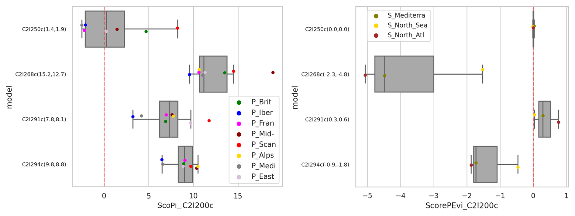
Figure 19 ScoPi_region based on the differences in the mean BIAS of all variables labelled with ScoPi weights in Table 2 defined for land points (left) and for ocean points, where only hfls_o contributes (right) between the observations and each simulation considered in the final decision (C2I250c, C2I268c, C2I291c, C2I294c), against the simulation C2I200c. The colours indicate the different CORDEX regions. The numbers given on the y-axis labels in brackets are the ScoPi_simulation. The values represent the averages over all eight regions weighted by the distance to Mid-Europe (first value), and by their area (second value) respectively (see Table 3). For the additional details see Sect. 2.6.1

The ScoPi of the revised reference C2I250c suggests that the changes in external data sets and updates in model versions do not influence the mean model quality but have impacts on the regional distribution of the biases for the land quantities only.

The expert and LiMMo tuned configurations reveal relatively high positive ScoPi values, indicating significant improvements in simulation quality. The best performing simulation for the land quantities is the expert tuned configuration C2I268c (11.5 points), followed by the LiMMo tuned configuration C2I294c with low weight for hfls_o (9 points) and C2I291c with high weight for hfls_o (7 points). The improvements are found for all PRUDENCE regions with the weakest ScoPis over the Iberian Peninsula.

The LiMMo tunings C2I291c and C2I294c do not achieve the same model quality as expert tuning C2I268c with respect to ScoPi over land (Fig. 19, left). This, however, is not showing that the expert tuning outperforms LiMMo tuning. It shows that the additional constraint of LiMMo tuning, the reduction of the bias of latent heat flux bias over water (hfls_o is reducing the quality over land, as shown by ScoPi considering land points only. However, the analysis of hfls_o-based ScoPi reveals the weak performance in simulating latent heat flux with C2I268c and C2I294c.

3.5.2 Seasonal RMSE analysis

Figure 20 shows the time mean spatial RMSE with respect to observations and all variables considered in the LiMMo optimisation separately for the winter (a), the summer (b) and for all months (c). The values are normalised by the RMSE of C2I200c and shown as percentages. The intrinsic uncertainties of the model (see Eq. 6 and Table 4) are given as vertical whiskers. This allows to assess the statistical significance of the tuning.

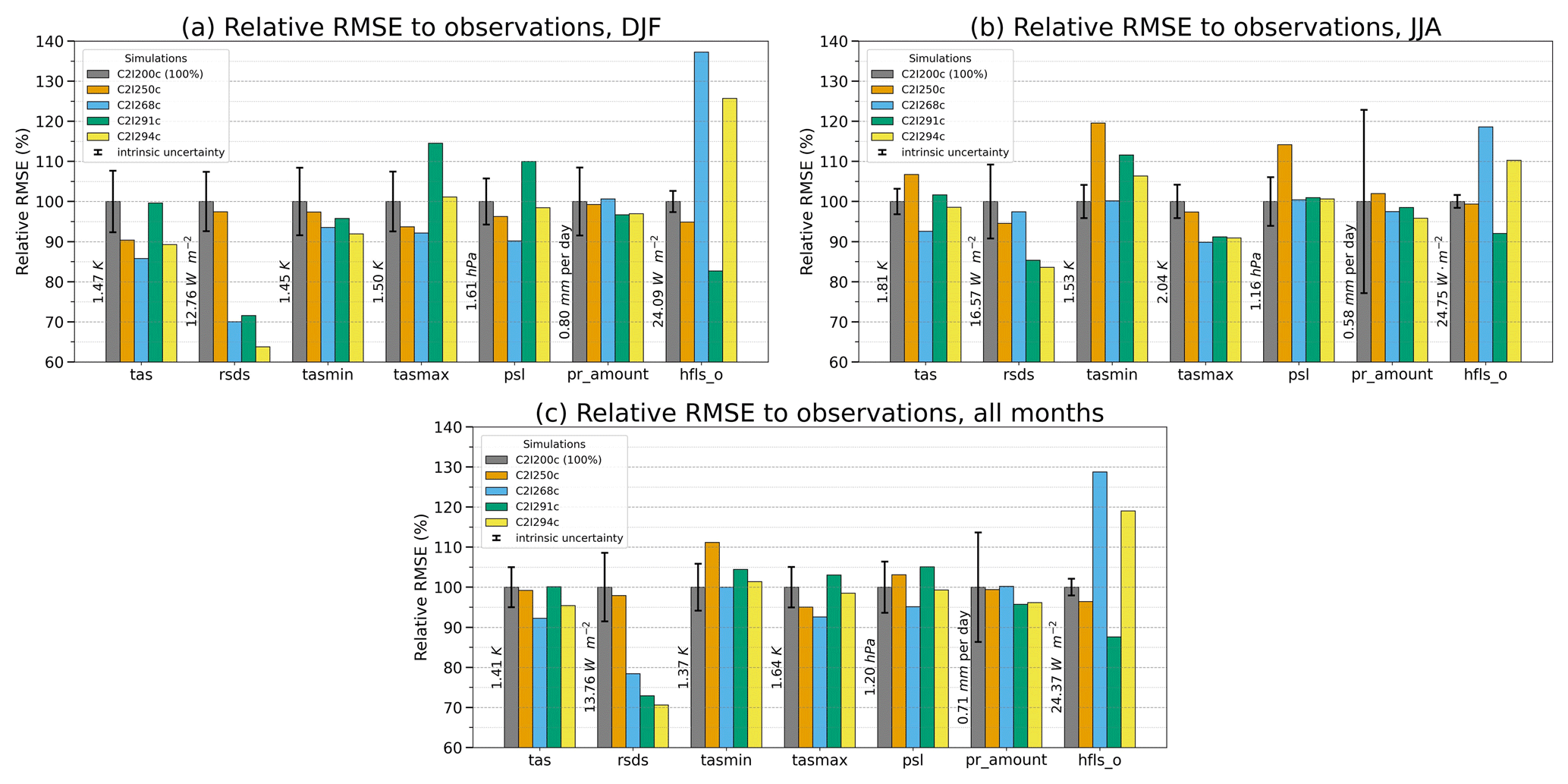
Figure 20 The Root Mean Square (RMS) difference between the model output and observations for different optimised ICON-CLM configurations averaged for (a) winter (DJF), (b) summer (JJA), and (c) all months in the climatological year. RMSE values are displayed for different model quantities (horizontal axis). The vertical whisker reflects the model's intrinsic uncertainty (Eq. 6, mean values for selected months). All RMSE values and intrinsic uncertainties are normalised to the RMSE for the initial configuration (first bar – C2I200c) for each model quantity. The absolute values of the RMSEs for the C2I200c are shown vertically to the left of the first bar for each model variable. Bars for all model quantities used in LiMMo tuning (see Table 2) are displayed.

First, we could not find a significant change in precipitation RMSE for any of the optimised configurations (see Fig. 20c for pr_amount). The changes of pr_amount in both winter and summer RMSE are also below the level of significance (see Fig. 20a and b for pr_amount). This can be explained by the relatively low sensitivity of pr_amount to parameter changes considered (see Fig. 2, column pr_amount). The initial configuration C2I200c has decent precipitation quality because a similar configuration is used for NWP. Therefore, the precipitation quality of the optimised configurations can be regarded as satisfactory.

Second, the expert optimised configuration C2I268c shows statistically significant improvement of RMSE for tas and tasmax in winter and summer. The LiMMo optimised configuration C2I294c (low weight of hfls_o, see Table 8) also reduces the RMSE significantly for tas in winter and for tasmax in summer. The second LiMMo configuration C2I291c (high weight of hfls_o, see Table 8) exhibits a different result. In winter, the tasmax RMSE is significantly increased. In summer, it is significantly reduced. For tasmin, the opposite holds – there is a slight decrease in winter and a significant increase in summer. The slightly reduced quality (5 %–10 % higher RMSE in comparison with C2I294c) of summer tasmin and winter tasmax affects climatologically relevant quantities like the number of tropical nights and frost days. This can be accepted for regional climate applications, considering the significant improvement in winter tasmin and summer tasmax, improving the quality of winter cold nights and summer hot days. It allows for keeping or even improving the predictability of cold events in winter and heat waves in summer, which are usually of the main interest for the risk assessments.

Third, Fig. 20 shows significant and strong differences in rsds and hfls_o (for optimised configuration with respect to C2I200c). The results are similar for C2I200c and C2I250c. Thus, updating the external parameters has a minor impact on these quantities. A large and significant decrease of up to 30 % in rsds RMSE was found for the expert (C2I268c) and LiMMo-optimised (C2I291c, C2I294c) configurations with 30 % to 35 % in winter for all three and about 15 % to 20 % in summer for the LiMMo configurations only.

Fourth, the rsds RMSE reductions in C2I268c and C2I294c are accompanied by a significant and strong increase of the hfls_o RMSE (30 % to 40 % in winter and 10 % to 20 % in summer). The C2I291c configuration, however, is the only one showing a significant and strong reduction of hfls_o RSME in both seasons (∼ 17 % in winter and ∼ 7 % in summer).

3.5.3 2D seasonal BIAS analysis

In the current section, we show the seasonally averaged 2-dimensional bias plots for the most significant changes identified in the RMSE analysis (see Fig. 20 in Sect. 3.5.2).

First, we compare the 2-dimensional biases of summer tasmin and winter tasmax for configurations C2I200c, C2I250c, and C2I291c in the Fig. 21 to ensure that there are no severe violations of the model quality by the configuration changes in these quantities. The update of the external data sets leads to an overall positive temperature shift in summer tasmin (Fig. 21b vs. a). The LiMMo tuning slightly reduces the summer tasmin bias, especially in central Europe and northern Africa (Fig. 21c vs b), but the bias still remains overall positive and larger than in the original setup (Fig. 21c vs. a). The positive temperature shift is visible for winter tasmax as well (Fig. 21e vs. d), slightly reducing the negative bias. However, the LiMMo tuning reverses this improvement, leading to a slightly stronger negative bias (Fig. 21f vs. d). This degradation is mainly confined to the northern African region. Overall, the quality of the summer tasmin and winter tasmax can be regarded as similar in C2I291c and C2I200c, especially for the target region of central Europe.

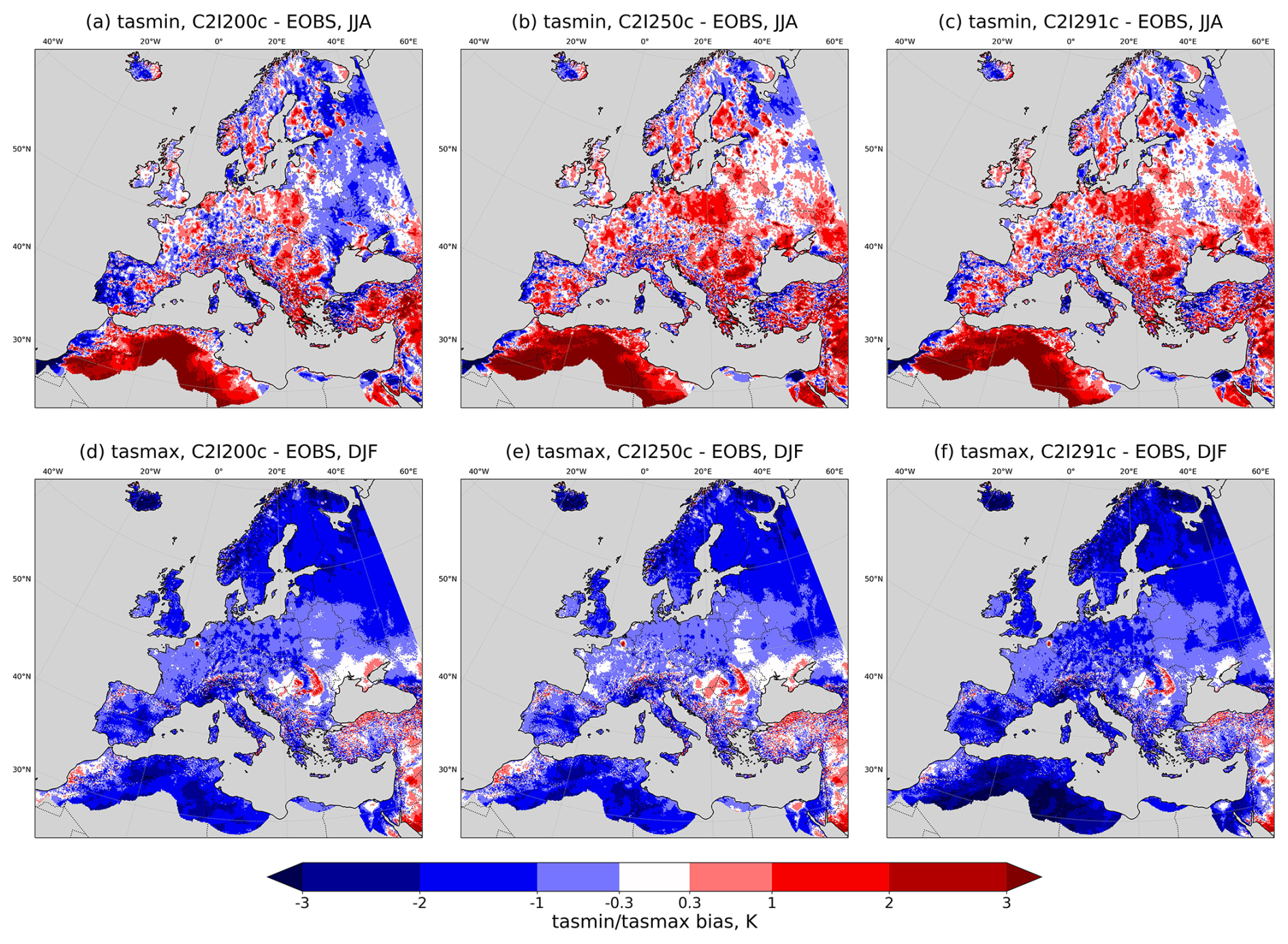
Figure 21 Seasonal biases (2003–2008) for summer tasmin (top) and winter tasmax (bottom) for configurations C2I200c, C2I250c and C2I291c compared to E-OBS.

Second, in Fig. 22 we present the summer rsds and winter hfls_o biases for C2I200c, C2I268c, and C2I291c. The LiMMo parameter tuning clearly reduces the positive rsds bias over central and western Europe while slightly increasing it in Eastern Europe (Fig. 22c vs. a). The expert tuning results in an enhanced negative bias over central and eastern Europe (Fig. 22b vs. a), while slightly reducing the positive bias in Western Europe. Along with the ambiguous performance for rsds, we observe a strong degradation of winter hfls_o of 10 W m⁻² in the Expert configuration C2I268c (Fig. 22e vs. d). The LiMMo configuration C2I291c provides clearly reduced bias in the Atlantic and Mediterranean (Fig. 22f vs. d). A comprehensive analysis of seasonal 2D biases for tas, tasmin, tasmax, rsds, hfls_o, pr_amount and psl is provided in the supplementary materials (see Sect. S5).

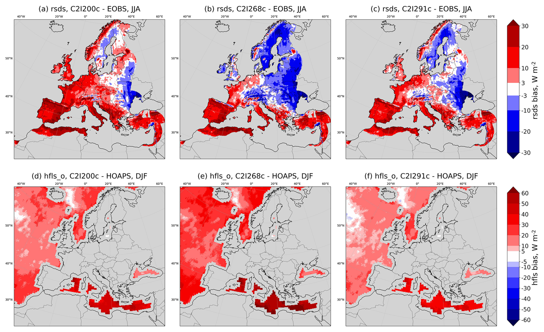
Figure 22 Seasonal biases (2003–2008) for summer rsds (top) and winter hfls_o (bottom) for configurations C2I200c, C2I268c and C2I291c compared to E-OBS and HOAPS, respectively.

3.6 Recommended optimised configuration

The evaluation results show that the optimised configuration C2I268c, obtained by expert tuning, and C2I291c and C2I294c, obtained by LiMMo tuning, exhibit a significant reduction of overestimation of incoming solar radiation at the surface, i.e., they reach one of the tuning aims. Additionally, the configuration C2I268c shows a significant reduction of tas bias. However, the Expert configuration C2I268c and the LiMMo configuration C2I294c with low weight of hfls_o exhibit a much increased hfls_o bias (+25 %, Fig. 20c) in comparison with C2I200c. The LiMMo configuration C2I291c is the only one which reveals major improvements in incoming short wave radiation at the surface rsds (30 % reduction of rsds RMSE, Fig. 20c) and latent heat flux over the ocean hfls_o (12 % reduction of hfls_o RMSE, Fig. 20c). This improvement is accompanied by a statistically significant worsening of tasmax in the winter season only (+15 % in winter tasmax RMSE, Fig. 20a).

In expert tuning, five parameters were tuned. In LiMMo tuning, ten parameters were tuned. A comparison of the tuned parameter values from the optimised expert and LiMMo configurations (Table 10) reveals differences higher than 10 % of the parameter value in the cloud condensation parameter tune_box_liq, in resistance parameters of turbulent fluxes over land (rlam_heat) and oceans (𝚛𝚊𝚝_𝚜𝚎𝚊⋅𝚛𝚕𝚊𝚖_𝚑𝚎𝚊𝚝), in the factor of minimum stomata resistance to transpiration (rsmin_fac) and in the correction of dry soil albedo (tune_albedo_wso(1)).

The parameter sensitivities given in Fig. 2 indicate that the reduction of the error in hfls_o is related to 𝚛𝚊𝚝_𝚜𝚎𝚊⋅𝚛𝚕𝚊𝚖_𝚑𝚎𝚊𝚝. Since the value 5 is found to be a lower limit of physically meaningful values, the value 9.7 in C2I291c can be regarded as physically well justified. The parameter tune_box_liq has a much smaller sensitivity than tune_box_liq_asy and allow_overcast, and thus it can be regarded as less important. The stomata resistance factor exhibits no sensitivity, and its increase by 30 % is thus physically acceptable as well. The albedo increase for dry soils is found half size in LiMMo in comparison with the optimised Expert configuration and thus physically even more acceptable.

All in all, the LiMMo configuration is closer to the reference configuration and physically more reliable than the optimised Expert configuration. This confirms the evaluation results. Therefore, we recommend using the LiMMo tuned configuration C2I291c with the high weight of hfls_o.

For climate change applications, we recommend using the urban parametrisation terra_urb additionally. Urban areas contribute only marginally to regional means and do not affect the consistency with E-OBS, as inner city stations are excluded there. But the parameterisation is important to capture the urban heat island effects.

Table 10 Reference simulations and all configurations used in the final decision making. Rows: tuning parameters (see Tables 5 and 6); columns: simulation IDs (see Table D1). The settings marked with “^*” are given in Table A2. If the value in a cell is missing, it is replaced with its neighbouring value to the left.

4 Summary and Conclusions

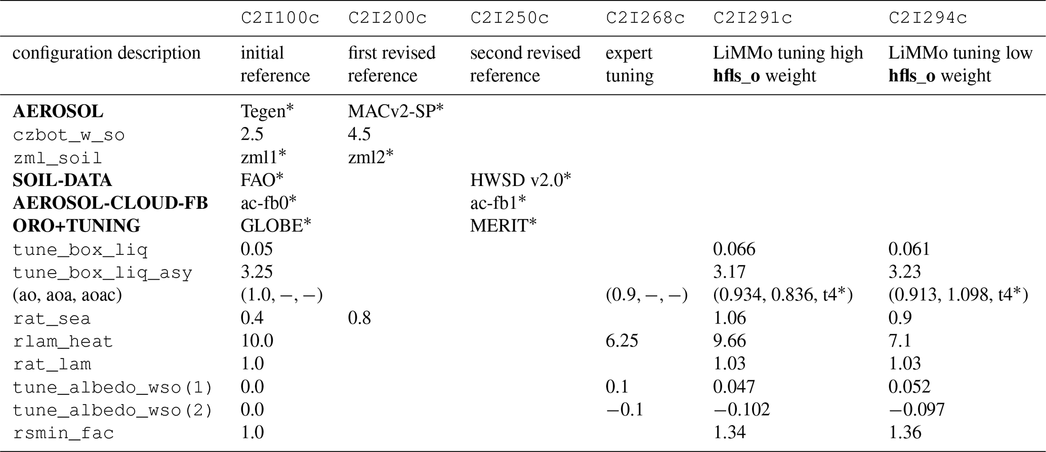
In this paper, we introduce a strategy and concrete procedures for tuning regional climate models. The generic framework was used to derive an optimised configuration for the ICON model in climate limited-area mode (ICON-CLM) for the CORDEX pan-European model domain at 12 km (EUR-12) grid resolution. The RCM tuning strategy presented here is a significantly improved procedure compared to the one previously used for the COSMO-CLM. This tuning strategy comprised parameter testing, revision of the reference configuration by expert judgement, configuration optimisation using expert tuning and an assessment of the optimised configurations using the ScoPi measure (Geyer, 2026). In the present study, this was extended by the application of the novel Linear Meta-model (LiMMo) tuning framework. It adds value to the overall procedure as it can be seamlessly combined with, or used instead of, expert tuning. Furthermore, it can substantially extend the optimisation space by optimising a large number of parameters, since the number of the simulations required for the LiMMo tuning is equal to the number of tuned parameters plus three.

Aside from an optimised model configuration, targeted to a specific optimisation goal, we present and discuss the model parameter sensitivities, which are the basis of the optimisation procedure.

Following the tuning strategy, the results of its application to ICON-CLM can be summarised as follows:

• First, the tuning aim was determined from the reference simulation assessment. The analysis revealed a 1.5 K cold bias in 2 m-temperature, an overestimation of incoming surface solar radiation by more than 10 W m⁻², and an overestimation of latent heat flux over the ocean surface by more than 15 W m⁻² in spatial and yearly means. The reduction of these biases was determined to be the tuning aim.

• Second, new external data sets for soil type (HWSD v2.0), orography (MERIT), and transient aerosols (MACv2-SP) have been incorporated for the first time. The revised reference configuration (by expert judgement) became the basis for the further testing of model parameters. The sensitivity of model results on parameters of cloud cover dependency on atmospheric water content, of vertical mixing, convection, and of surface fluxes were investigated. Two new parameters of soil moisture dependence of surface albedo and two of plant transpiration and evaporation have been tested. The test simulation results have been evaluated for key model quantities: tas, tasmin, tasmax, rsds, pr_amount, hfls_o, and psl. The discussion of the model response revealed sometimes counter-intuitive, but physically consistent model behaviour. The majority of parameters have been shown to have a model sensitivity that is significantly higher than the intrinsic model variability.

• Third, we determined an optimised configuration by expert tuning. Hereby up to six out of twelve sensitive tuning parameters have been adjusted, which have been found to exhibit a sensitivity correlated with substantial parts of the model bias. The optimised Expert configuration has been shown to reduce errors by 8 % for tas and tasmax, 20 % for rsds, and to increase hfls_o errors by 30 %.

• Fourth, we applied LiMMo tuning, which is based on a linear emulator of monthly mean values and optimisation of the error norm consisting of weighted signal-to-noise ratios for model variables. We considered the results of tuning twelve sensitive model parameters using two sets of weights for model variables in LiMMo. The ICON-CLM simulations with LiMMo-derived configurations confirmed the bias reductions found by the meta-model.

The optimisation of all twelve tuning parameters in LiMMo tuning allowed us to find a configuration with a smaller error norm than in expert tuning. However, the model error reduction remained limited to a few variables (30 % reduction of rsds and 15 % reduction of hfls_o yearly mean RMSE). This indicates that a further error reduction might be impossible only by existing parameter tuning without further model development.

The LiMMo configuration, which was obtained for the low weight of hfls_o, shows a quality similar to that found by expert tuning. The LiMMo configuration for a high weight of hfls_o reduces the error norm of incoming solar radiation by 30 % and of latent heat flux over water by 15 % while keeping the simulation quality of temperature, pressure, and precipitation similar to the reference (insignificantly worse). This also demonstrates the possibility of controlling the tuning result by the user. The method's linear computational complexity allows it to be extremely efficient, yielding results in just a few minutes. This is one of the strengths, combined with the relatively small number of simulations needed.

We consider a combination of expert tuning, a step-wise improvement of reference configurations, in combination with LiMMo (fine-tuning) as a best practice RCM tuning strategy.

The new ICON-CLM configuration for climate mode applications with a spatial resolution of 12 km over the European region, as determined by the hybrid expert-LiMMo tuning, is already in use, e.g., by the CLM-Community for WCRP CORDEX-CMIP6 EURO-CORDEX climate change simulations.

Appendix A: Namelist parameter descriptions

Coddington et al. (2016)Coddington et al. (2016)Schlemmer et al. (2018)Wouters et al. (2016)

Table A1 Description of namelist parameters changed in the optimisation process; the full list of namelist parameters for ICON can be accessed at https://gitlab.dkrz.de/icon/icon-model/-/tree/release-2025.04-public/doc/Namelist_overview (last access: 3 June 2025).

Table A2 Description of the parameter settings abbreviated in Tables 5, 6, 7, 9 and 10.

Appendix B: Additional technical information on experiment setups

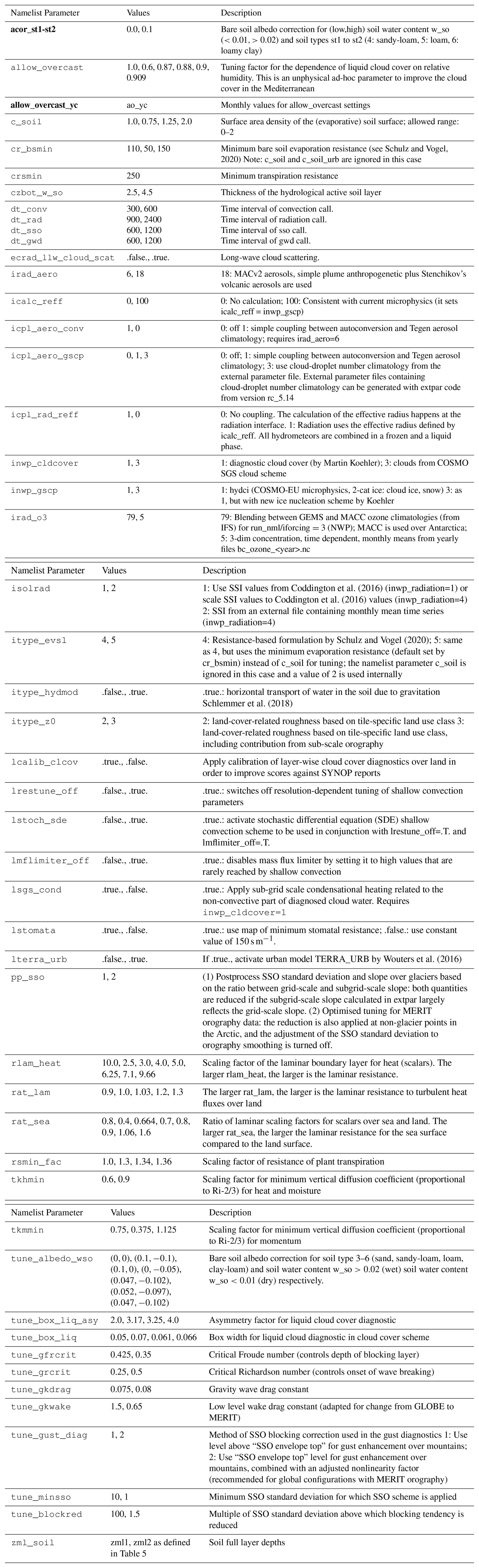
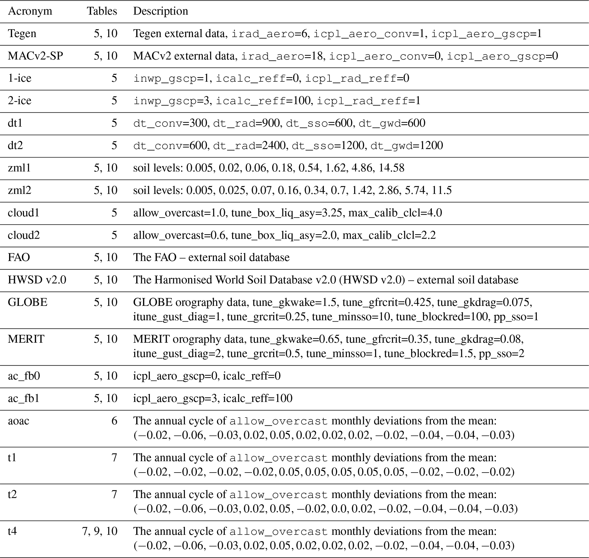
Table B1 Overview of periods used for simulation, analysis, and optimisation.

(Schlemmer et al., 2018)

Table B2 Overview of used model versions.

Appendix C: Experiments for the definition of the new reference

Schlemmer et al. (2018)

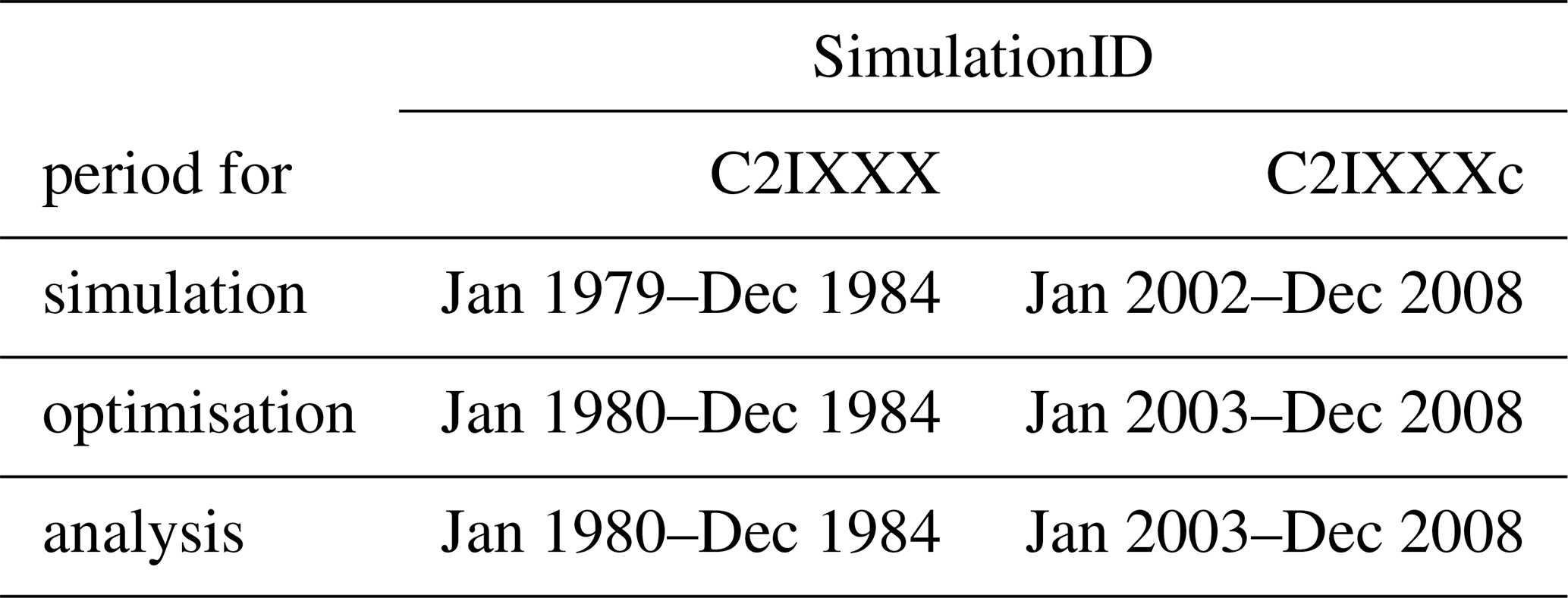
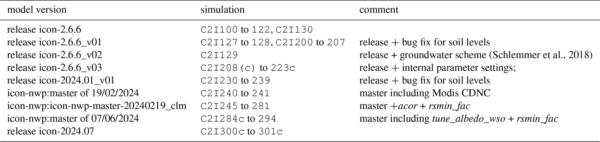
Table C1 Description of changes in the model setup of different experiments to define a new reference compared to the initial reference experiment C2I101. n/a: not applicable.

Appendix D: Further sensitivity test experiments and simulations with configurations by expert and LiMMo tuning

Table D1 Description of changes in the model setup of further sensitivity studies and the configurations proposed by expert and LiMMo tuning with respect to their reference experiment. n/a: not applicable.