Automatic tuning of iterative pseudo-transient solvers for modeling the deformation of heterogeneous media

Geodynamic modeling has become a crucial tool for investigating the dynamics of Earth deformation across various scales. Such simulations often involve solving mechanical problems with significant material heterogeneities (e.g. strong viscosity contrasts) under nearly incompressible conditions. Recent advancements have enabled the development of iterative solvers based on Dynamic Relaxation (DR) or Pseudo-Transient schemes, which require minimal global communication and exhibit quasi-linear scaling on GPU and supercomputing architectures. These solvers incorporate automatic tuning of iterative parameters, including pseudo-time steps and damping coefficients, based on spectral estimates of the discrete operators, ensuring both robust and rapid convergence. We demonstrate the effectiveness of this approach on discretized problems with finite-difference and face-centered finite volume methods, including heterogeneous incompressible Stokes flows. Moreover, the relative algorithmic simplicity of DR-based methods allows straightforward extensions to compressible flow, multiphase flow, and nonlinear constitutive laws, opening promising avenues for large-scale, high-resolution simulations of geoscientific problems.

1 Introduction

Geodynamic modeling has become an indispensable tool for simulating tectonic processes at various scales, ranging from the rock sample (e.g. Luisier et al., 2023) and outcrop levels (e.g. Schmalholz and Podladchikov, 2001) to regional (Gerya, 2013), global (e.g. Fuchs and Becker, 2022), and planetary scales (e.g. Tackley, 2023). Geodynamic modeling tools aim to solve the conservation equations of linear momentum, mass, and energy to produce full-field solutions for velocity, pressure, and temperature fields in space and time (Gerya, 2019).

While 2D geodynamic simulations can effectively leverage solvers that employ sparse-direct or direct-iterative schemes (e.g. Dabrowski et al., 2008; Gerya and Yuen, 2003; Fullsack, 1995; Popov and Sobolev, 2008), 3D simulations generally require iterative solvers as direct methods become prohibitively expensive. Most approaches in this context rely on multigrid solvers (e.g. May et al., 2015; Tackley, 1996; Kronbichler et al., 2012; Kaus et al., 2016; Baumgardner, 1985; Zhong et al., 2008; Shih et al., 2022), spectral methods (e.g. Balachandar and Yuen, 1994), or pseudo-transient integration techniques (Duretz et al., 2019; Räss et al., 2022) to achieve efficient solutions.

In geodynamic models, the viscosity field may exhibit smooth (i.e. thermal variations) and sharp (i.e. material interfaces) spatial variations of several orders of magnitude. This peculiarity makes the iterative solution procedure of the near-incompressible and incompressible Stokes equation particularly challenging (e.g. Tackley, 1996; May et al., 2015; Räss et al., 2022; Shih et al., 2022).

Iterative solvers based on pseudo-transient integration or Dynamic Relaxation (DR) have been employed to solve compressible and incompressible geomechanical and geodynamical problems (e.g. Cundall and Board, 1988; Poliakov et al., 1993; Hassani et al., 1997). These methods exhibit interesting parallel scaling properties on hardware accelerators such as Graphics Processing Units (GPU) and have therefore recently been applied to study incompressible Stokes flow and multi-physics coupled problems (e.g. Räss et al., 2022; Duretz et al., 2019; Räss et al., 2019; Halter et al., 2022; Spang et al., 2025). These solvers implement coupled solving strategies that involve iterative updates of both the velocity and pressure fields within a single iteration loop. Despite their algorithmic simplicity, their application to heterogeneous mechanical problems remains challenging (e.g. Halter et al., 2022). One strategy relies on smoothing sharp contrasts in material properties; however, this approach requires the use of a very fine spatial resolution to match exact flow solutions (e.g. Räss et al., 2022; Halter et al., 2022). In practice, Stokes solvers are typically coupled with Marker-In-Cell or Level-Set approaches (e.g. Gerya and Yuen, 2003; Hillebrand et al., 2014; Samuel and Evonuk, 2010; Schmeling et al., 2008) to handle large viscous deformations and to represent heterogeneous materials. In the latter case, the degree to which discontinuities in material properties are smoothed depends on the spatial extent (or support) of the interpolant basis functions (e.g. Duretz et al., 2011). The degree of smoothing is therefore not defined ad hoc and must be based on a narrow interpolation basis to best match the exact flow solution (Duretz et al., 2011). Moreover, current geodynamic pseudo-transient solvers rely on either empirical tuning of iterative parameters (e.g. Duretz et al., 2019) or exact derivation of optimal parameters based on simplified model configurations (e.g. Räss et al., 2022; Alkhimenkov et al., 2021). This situation hinders their applicability in solving “real-life” geodynamic problems, as optimal parameters may adapt to the evolving internal model state and material configuration. Exploring dynamic strategies to select optimal iterative parameters is a motivation to overcome current limitations.

In this study, we aim to solve quasi-steady mechanical problems with large and sharp variations in material properties using DR-like iterative solvers and automatic tuning of iterative parameters. We present a decoupled solution strategy that combines Schur-complement reduction, Powell–Hestenes iterations, and DR-type of iterative solvers.

2 Mechanical equilibrium

The equations governing quasi-static mechanical equilibrium in a classical continuum medium may be expressed as:

$$\begin{array}{}\text{(1)}& {\displaystyle }\mathbf{\nabla }\cdot \mathit{\tau }-\mathbf{\nabla }P-\mathit{b}=\mathbf{0},\text{(2)}& {\displaystyle }\mathbf{\nabla }\cdot \mathit{v}+{\displaystyle \frac{\mathrm{1}}{K}}{\displaystyle \frac{\mathrm{d}P}{\mathrm{d}t}}=\mathrm{0}.\end{array}$$

where τ is the deviatoric stress tensor, P is pressure, and v is the velocity vector. The term $\mathit{b}=-\mathit{\rho }\mathit{g}$ is a forcing term, where ρ, g and K correspond to density, gravitational acceleration, and bulk modulus, respectively. The incompressible limit is reached if K→∞. The isotropic viscous constitutive relationship takes the form of:

$$\begin{array}{}\text{(3)}& \mathit{\tau }=\mathrm{2}\mathit{\eta }\dot{\mathit{\epsilon }}=\mathrm{2}\mathit{\eta }\left[\mathbf{D}-{\displaystyle \frac{\mathrm{1}}{\mathrm{3}}}(\mathbf{\nabla }\cdot \mathit{v})\mathbf{I}\right],\end{array}$$

where $\dot{\mathit{\epsilon }}$ is the deviatoric strain rate tensor, $\mathbf{D}=\mathrm{1}/\mathrm{2}\left(\mathbf{\nabla }\mathit{v}+(\mathbf{\nabla }\mathit{v}{)}^T\right)$, I is the identity matrix and η is the dynamic viscosity. In the following, the Stokes equations will be solved for velocity and pressure fields over a domain Π, accounting for Neumann boundary conditions ($\mathit{\sigma }\cdot \mathit{n}={\mathbf{T}}_{\mathrm{N}}$) on the boundary ∂Π_N and Dirichlet boundary conditions (v=v_D) on the boundary ∂Π_D.

3 Discretizations

We consider two different types of numerical discretization of the Stokes equations, the staggered-grid Finite-Difference (FD) and Face-Centered Finite Volume (FCFV) Method. With either discretization, both the components of the velocity vector and the pressure will constitute the primitives, which we aim to solve for.

3.1 Staggered-Grid Finite-Differences Method

The staggered-grid finite-difference is a popular approach to discretizing the Stokes equation originally proposed by Harlow and Welch (1965). This scheme is constructed using conservative second-order finite difference and a staggered arrangement of both velocity and pressure (Fig. 1a, b). The strong form of the Stokes equations (Eq. 2) is discretized using central finite differences:

$$\begin{array}{}\text{(4)}& {\displaystyle }{\mathit{r}}_{\mathrm{mom}}=\widehat{\mathbf{\nabla }}\cdot \mathit{\tau }-\widehat{\mathbf{\nabla }}P-\mathit{b},\text{(5)}& {\displaystyle }{r}_{\mathrm{cont}}=-{\displaystyle \frac{\mathrm{1}}{K}}{\displaystyle \frac{\widehat{\mathrm{\Delta }}P}{\widehat{\mathrm{\Delta }}t}}-\widehat{\mathbf{\nabla }}\cdot \mathit{v},\text{(6)}& {\displaystyle }\mathit{\tau }=\mathrm{2}\mathit{\eta }\left[\widehat{\mathbf{D}}-{\displaystyle \frac{\mathrm{1}}{\mathrm{3}}}(\widehat{\mathbf{\nabla }}\cdot \mathit{v})\mathbf{I}\right],\end{array}$$

where the hat symbol denotes the discrete representation of the differential operators. The primitive solution fields v and p are obtained by minimizing the momentum and continuity residuals (r_mom and r_cont). The staggered FD scheme represents, to our knowledge, the most computationally efficient stencil that satisfies the Inf-Sup stability condition in regular meshes (Shin and Strikwerda, 1997). For flows with smooth viscosity variations, FD achieves second-order accuracy in the L1 norm, while in the presence of sharp material heterogeneities, its accuracy reduces to first-order (Duretz et al., 2011). Geometrically, FD has been successfully implemented in Cartesian and polar coordinates (e.g. Räss et al., 2017), spherical configurations (e.g. Tackley, 2008; Macherel et al., 2024), and on adaptively refined meshes (e.g. Gerya, 2013; Goldade et al., 2019). However, its application in non-orthogonal meshes remains rare (e.g. de la Puente et al., 2014) due to the need for extended stencils and the associated increase in algorithmic complexity. Consequently, the treatment of free-surface boundary conditions remains a notable challenge (e.g. Duretz et al., 2016; Larionov et al., 2017; Gray et al., 2025).

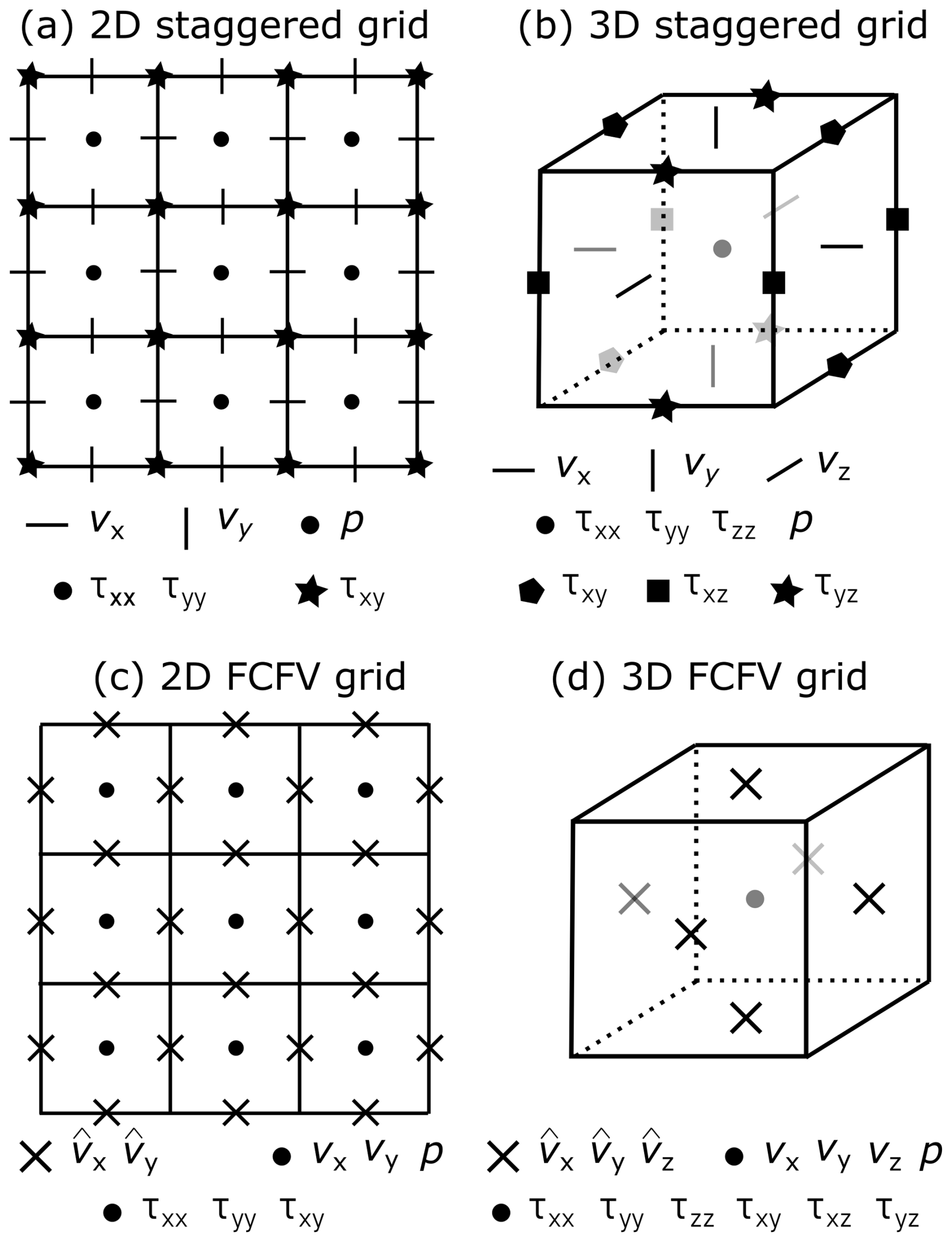
Figure 1 Grids employed for the discretization of mechanical problems. (a) 2D FD staggered grid, (b) 3D staggered grid, (c) 2D FCFV grid and (d) 3D FCFV grid.

3.2 Face-Centered Finite Volume Method (FCFV)

The Face-Centered Finite-Volume (FCFV) method is an emerging discretization scheme rooted in the principles of the hybridizable discontinuous Galerkin (HDG) method (Cockburn and Gopalakrishnan, 2005). This approach has been successfully employed to achieve full-field solutions for the Stokes equations in various types of viscosity distribution, including constant (Sevilla et al., 2018), discontinuous (Sevilla and Duretz, 2023), and smoothly varying fields (Sevilla and Duretz, 2024). The FCFV scheme satisfies the Inf-Sup stability condition, making it particularly suitable for solving the Stokes equations. The discrete system of equations is derived from the weak formulation of the Stokes problem, using a constant degree of approximation for both velocity and pressure fields:

$$\begin{array}{}\text{(7)}& {\displaystyle }{\mathit{r}}_{\mathrm{mom}}=\mathrm{\Gamma }\left[\left(\left[\left[\mathit{\tau }\right]\right]+\left[\left[P\right]\right]\mathbf{I}\right)\mathit{n}+\mathrm{2}s\left(\mathit{\left\{}\mathit{\right\{}\mathit{v}\mathit{\left\}}\mathit{\right\}}-\widehat{\mathit{v}}\right)-\mathit{\chi }{\mathbf{T}}_{\mathrm{N}}\right],\text{(8)}& {\displaystyle }{r}_{\mathrm{cont}}=-\sum _{i=\mathrm{1}}^{n_{\mathrm{fac}}}{\mathrm{\Gamma }}_i\left({\displaystyle \frac{\mathrm{1}}{K}}{\displaystyle \frac{\widehat{\mathrm{\Delta }}P}{\widehat{\mathrm{\Delta }}t}}+{\mathit{n}}_i\cdot {\widehat{\mathit{v}}}_i\right),\text{(9)}& {\displaystyle }\mathit{\tau }=\mathrm{2}\mathit{\eta }\left[\sum _{i=\mathrm{1}}^{n_{\mathrm{fac}}}{\displaystyle \frac{{\mathrm{\Gamma }}_i}{\mathrm{2}\mathrm{\Omega }}}\left({\mathit{n}}_i\otimes {\widehat{\mathit{v}}}_i+{\widehat{\mathit{v}}}_i\otimes {\mathit{n}}_i\right)-{\displaystyle \frac{\mathrm{1}}{\mathrm{3}}}{\mathit{n}}_i\cdot {\widehat{\mathit{v}}}_i\mathbf{I}\right],\text{(10)}& {\displaystyle }\mathit{v}={\displaystyle \frac{\mathrm{1}}{a}}\left(\mathit{b}\mathrm{\Omega }+\sum _{i=\mathrm{1}}^{n_{\mathrm{fac}}}{\mathrm{\Gamma }}_{i}s{\widehat{\mathit{v}}}_i\right),\end{array}$$

The primitive variables, namely the hybrid velocity vector ($\widehat{\mathit{v}}$) and pressure (P), are obtained by minimizing the momentum and continuity residuals (r_mom, r_cont). The hybrid velocity is an independent variable defined on element faces, different from the element-wise velocity. It serves as a Lagrange multiplier–type trace variable that enforces weak continuity of the velocity field across elements. The symbol n_fac corresponds to the number of faces of an element. [[⋅]] is the jump operator defined as $\left[\left[\odot \right]\right]={\odot }_{\mathrm{R}}-{\odot }_{\mathrm{L}}$, where ⊙ denotes quantities defined on elements located to the right (R) and left (L) of an interface. {{ ⋅ }} is the average operator defined as $\mathit{\left\{}\mathit{\right\{}\odot \mathit{\left\}}\mathit{\right\}}=\frac{\mathrm{1}}{\mathrm{2}}\left({\odot }_{\mathrm{R}}+{\odot }_{\mathrm{L}}\right)$. The discretization requires the outward-pointing normal to each face (n), the face area (Γ), the volume of the element (Ω), the stabilization parameter (s), the factor a ($a={\sum }_{i=\mathrm{1}}^{n_{\mathrm{fac}}}{\mathrm{\Gamma }}_{i}s$), the traction vector (T_N), and the function χ that indicates the presence of applied traction (0 or 1). The FCFV scheme requires the storage of the hybrid velocity vector and momentum residual at the midpoint of each element face, while the pressure, the deviatoric stress tensor and the continuity residual are stored in the centroids of the elements (Fig. 1c, d). The discretization considered here yields a first-order approximation of velocity and pressure fields (Sevilla et al., 2018), nevertheless second-order solutions can be constructed without altering the sparsity of the discretization (Giacomini and Sevilla, 2020; Vieira et al., 2020). In this study, we implement the FCFV approach using structured quadrangular meshes, although the method is versatile and supports arbitrary element geometries, exhibiting low sensitivity to mesh distortions (Sevilla et al., 2018). Additionally, FCFV can naturally handle internal boundaries and traction boundary conditions, such as free surfaces. Due to these features, the FCFV method is becoming increasingly popular in the geodynamics community, as highlighted by Burcet et al. (2024).

4 Dynamic Relaxation with automatic tuning

In this section, we discuss the principles behind the Dynamic Relaxation method and illustrate its basic properties using a simple 1D Poisson example.

4.1 Principle

The dynamic relaxation method is designed to iteratively solve both linear and nonlinear problems. The iterative procedure resembles an explicit time integration scheme, which is why it is also often referred to as a pseudo-transient integration method. As in classical iterative procedures, the DR method iteratively refines the unknown u until the magnitude of the residual of the partial differential operator r(u) drops below a given tolerance. Once this criterion is met, u is considered a solution satisfying r(u)=0. Note that the function r(u) may include physical transient terms; thus, this method is not limited to solving quasi-static problems (e.g. Räss et al., 2022). The algorithm is formulated by introducing the first and second-order derivative of the solution u in pseudo-time (Frankel, 1950):

$$\begin{array}{}\text{(11)}& \mathbf{M}{\displaystyle \frac{{\mathrm{d}}^{\mathrm{2}}\mathit{u}}{\mathrm{d}{\stackrel{\mathrm{‾}}{t}}^{\mathrm{2}}}}+\mathbf{M}c{\displaystyle \frac{\mathrm{d}\mathit{u}}{\mathrm{d}\stackrel{\mathrm{‾}}{t}}}=\mathit{r}\left(\mathit{u}\right)\end{array}$$

where $\stackrel{\mathrm{‾}}{t}$ refers to pseudo-time, c is a damping parameter, and M is a preconditioner. Following previous work (e.g. Papadrakakis, 1981; Oakley and Knight, 1995), the second derivative is taken as the central derivative of the first derivative and the first derivative is taken as the average of the new and old values:

$$\begin{array}{}\text{(12)}& {\displaystyle \frac{{\mathrm{d}}^{\mathrm{2}}\mathit{u}}{\mathrm{d}{\stackrel{\mathrm{‾}}{t}}^{\mathrm{2}}}}\approx {\displaystyle \frac{\mathrm{1}}{\mathrm{\Delta }\stackrel{\mathrm{‾}}{t}}}\left({{\displaystyle \frac{\mathrm{\Delta }\mathit{u}}{\mathrm{\Delta }\stackrel{\mathrm{‾}}{t}}}}^{\mathrm{new}}-{{\displaystyle \frac{\mathrm{\Delta }\mathit{u}}{\mathrm{\Delta }\stackrel{\mathrm{‾}}{t}}}}^{\mathrm{old}}\right)\text{(13)}& {\displaystyle \frac{\mathrm{d}\mathit{u}}{\mathrm{d}\stackrel{\mathrm{‾}}{t}}}\approx {\displaystyle \frac{\mathrm{1}}{\mathrm{2}}}\left({{\displaystyle \frac{\mathrm{\Delta }\mathit{u}}{\mathrm{\Delta }\stackrel{\mathrm{‾}}{t}}}}^{\mathrm{new}}+{{\displaystyle \frac{\mathrm{\Delta }\mathit{u}}{\mathrm{\Delta }\stackrel{\mathrm{‾}}{t}}}}^{\mathrm{old}}\right).\end{array}$$

This leads to update rules for the rate of change of u, and u itself:

$$\begin{array}{}\text{(14)}& {{\displaystyle \frac{\mathrm{\Delta }\mathit{u}}{\mathrm{\Delta }\stackrel{\mathrm{‾}}{t}}}}^{\mathrm{new}}=b{{\displaystyle \frac{\mathrm{\Delta }\mathit{u}}{\mathrm{\Delta }\stackrel{\mathrm{‾}}{t}}}}^{\mathrm{old}}+a{\mathbf{M}}^{-\mathrm{1}}\mathit{r}\left(\mathit{u}\right)\text{(15)}& {\displaystyle }{\mathit{u}}^{\mathrm{new}}={\mathit{u}}^{\mathrm{old}}+\mathrm{\Delta }\stackrel{\mathrm{‾}}{t}{{\displaystyle \frac{\mathrm{\Delta }\mathit{u}}{\mathrm{\Delta }\stackrel{\mathrm{‾}}{t}}}}^{\mathrm{new}}\end{array}$$

where $a=\mathrm{2}\mathrm{\Delta }\stackrel{\mathrm{‾}}{t}/(\mathrm{2}+c\mathrm{\Delta }\stackrel{\mathrm{‾}}{t})$ and $b=(\mathrm{2}-c\mathrm{\Delta }\stackrel{\mathrm{‾}}{t})/(\mathrm{2}+c\mathrm{\Delta }\stackrel{\mathrm{‾}}{t})$. Alternatively, the DR algorithm can be expressed in analogy to the conjugate gradient (CG) method (Feng, 2006), using the variable $\mathit{p}=\mathrm{\Delta }\mathit{u}/\left(\mathit{\beta }\mathrm{\Delta }\stackrel{\mathrm{‾}}{t}\right)$:

$$\begin{array}{}\text{(16)}& {\displaystyle }{\mathit{p}}^{\mathrm{new}}=\mathit{\beta }{\mathit{p}}^{\mathrm{old}}+{\mathbf{M}}^{-\mathrm{1}}\mathit{r}\left(\mathit{u}\right)\text{(17)}& {\displaystyle }{\mathit{u}}^{\mathrm{new}}={\mathit{u}}^{\mathrm{old}}+\mathit{\alpha }{\mathit{p}}^{\mathrm{new}}\end{array}$$

where p is analogous to the search direction, $\mathit{\alpha }=a\mathrm{\Delta }\stackrel{\mathrm{‾}}{t}$ and β=b. The main difference is that the CG method involves different expressions for the parameters α and β, which need to be reevaluated at each iteration, requiring computationally expensive reduction operations (e.g. vector norms).

In either case, two iteration parameters need to be determined as a function of the minimum (λ_min) and maximum (λ_max) eigenvalues of the discrete problem (Papadrakakis, 1981; Oakley and Knight, 1995):

$$\begin{array}{}\text{(18)}& {\displaystyle }\mathrm{\Delta }\stackrel{\mathrm{‾}}{t}=c_{\mathrm{CFL}}{\displaystyle \frac{\mathrm{2}}{\sqrt{{\mathit{\lambda }}_{\max }}}}\text{(19)}& {\displaystyle }c=c_{\mathrm{damp}}\mathrm{2}\sqrt{{\mathit{\lambda }}_{\min }}\end{array}$$

where c_CFL and c_damp are scalar adjustment parameters. Whereas c_CFL is strictly bounded (c_CFL<1), no analogous upper bound applies to c_damp. In our experiments, values in the range $\approx [\mathrm{0.5},\mathrm{1}]$ were found to provide robust performance. For optimal convergence, at least in the case of linear problems, c_CFL should be chosen as large as possible (e.g.  c_CFL=0.999). In theory (e.g. Oakley and Knight, 1995), the optimal value of c_damp is 1.0. Nevertheless, we empirically observed that slightly lower values may further enhance convergence.

The maximum eigenvalue is found using the Gershgorin circle theorem:

$$\begin{array}{}\text{(20)}& {\mathit{\lambda }}_{max}=\underset{i}{max}\left(\left|{\displaystyle \frac{\partial {\mathit{r}}_i}{\partial {\mathit{u}}_i}}\right|+\sum _{j\ne i}\left|{\displaystyle \frac{\partial {\mathit{r}}_i}{\partial {\mathit{u}}_j}}\right|\right).\end{array}$$

The minimum eigenvalue can only be approximated, using, for example, a Rayleigh quotient approach (e.g. Joldes et al., 2011; Rezaiee-Pajand and Sarafrazi, 2011; Oakley and Knight, 1995):

$$\begin{array}{}\text{(21)}& {\mathit{\lambda }}_{\min }=\left|{\displaystyle \frac{\mathrm{\Delta }{\mathit{u}}^T\mathrm{\Delta }\mathit{r}}{\mathrm{\Delta }{\mathit{u}}^T\mathbf{M}\mathrm{\Delta }\mathit{u}}}\right|,\end{array}$$

where $\mathrm{\Delta }\mathit{u}={\mathit{u}}^{\mathrm{new}}-{\mathit{u}}^{\mathrm{old}}$ and $\mathrm{\Delta }\mathit{r}=\mathit{r}\left({\mathit{u}}^{\mathrm{new}}\right)-\mathit{r}\left({\mathit{u}}^{\mathrm{old}}\right)$. The evaluation of iterative parameters requires two reductions. Reduction operations should be avoided when possible given that reduction algorithms in shared memory architectures are not embarrassingly parallel, and global communication between different nodes is needed in distributed memory architectures. Nevertheless, this procedure can be performed every n iterations, together with the evaluation of the stopping criteria. This approach provides successful convergence while minimizing the cost of global communication. It should be noted that the estimate of λ_min relies on differences in the residual. Before the iteration is initiated, this quantity is set to zero by default.

Lastly, the DR method requires the definition of a preconditioner, typically defined as the Jacobi or diagonal preconditioner:

$$\begin{array}{}\text{(22)}& \mathbf{M}=\mathrm{diag}\left({\displaystyle \frac{\partial \mathit{r}}{\partial \mathit{u}}}\right).\end{array}$$

While this choice allows for trivial inversion and parallelisation, it restricts the convergence property of the iteration scheme. In the context of matrix-free schemes, both the evaluation of the preconditioner and maximum eigenvalue estimates can be achieved by using automatic differentiation of the residual function.

4.2 Example: 1D Poisson problem

An example of the application of the DR method to a variable coefficient Poisson problem is depicted in Fig. 2. The problem is defined as:

$$\begin{array}{}\text{(23)}& {\displaystyle }\mathit{r}\left(\mathit{u}\right)=-\mathrm{\nabla }\cdot \mathit{q}-\mathit{b},\text{(24)}& {\displaystyle }\mathit{q}=-\mathit{k}\mathrm{\nabla }\mathit{u}\end{array}$$

where k=f(x). The differential operators are discretized with both the FD and the FCFV over a 1D domain $\mathrm{\Omega }=\left[-\frac{\mathrm{1}}{\mathrm{2}},\frac{\mathrm{1}}{\mathrm{2}}\right]$ and Dirichlet boundary conditions $u\left(-\frac{\mathrm{1}}{\mathrm{2}}\right)=\mathrm{1}$, $u\left(\frac{\mathrm{1}}{\mathrm{2}}\right)=\mathrm{2}$ (Fig. 2a). The coefficient k varies with x (Fig. 2b) and is expressed as

$$\begin{array}{rl}f\left(x\right)& =\mathrm{1}+\mathrm{100}({\left[\mathrm{1}+\exp (-\mathrm{200}(x+\mathrm{0.1}\left)\right)\right]}^{-\mathrm{1}}\\ & -{\left[\mathrm{1}+\exp (-\mathrm{200}(x-\mathrm{0.1}\left)\right)\right]}^{-\mathrm{1}}).\end{array}$$

The forcing term is set to zero so that b(x)=0. The problem converges for different resolutions to a relative residual of 10⁻¹⁰, with evaluation of iterative parameters and convergence check every 100 iterations. The frequency with which the parameters are reevaluated can influence the convergence behavior. In the present study, a value of 100 was empirically determined to provide an appropriate compromise. The typical convergence behavior of the DR method is shown in Fig. 2c. As a consequence of diagonal preconditioning, the number of iterations needed to reach convergence depends linearly on the size of the problem (Fig. 2d). It is worth noting that for the 1D Poisson case, the FD and the FCFV deliver very similar results, both in terms of the numerical solution and convergence behavior.

The DR method is particularly well-suited to solving symmetric positive-definite problems. The solution of indefinite problems, such as those arising in saddle-point systems such as the Stokes equations, requires additional modifications.

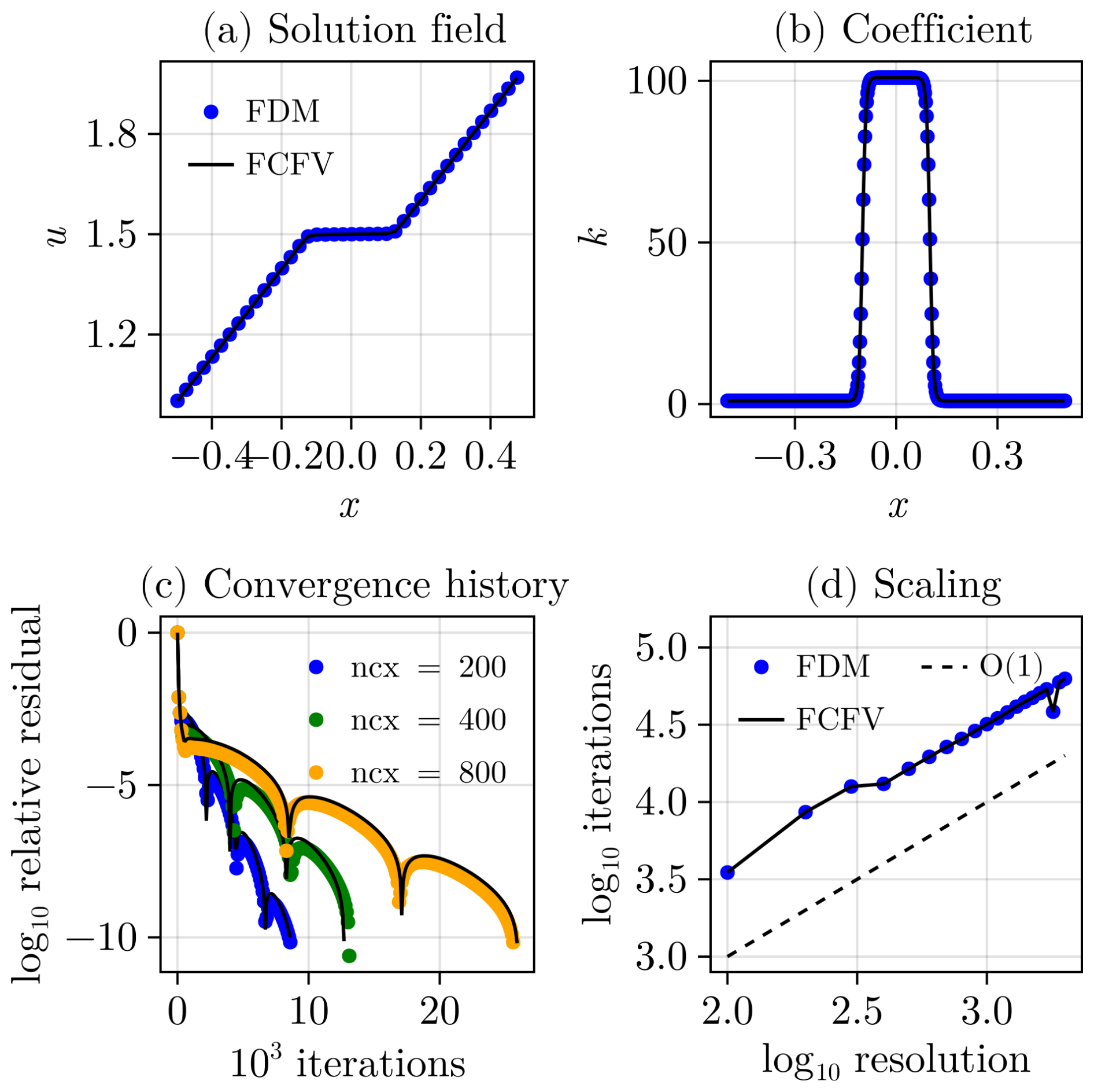
Figure 2 Properties of the DR method for the solution of a 1D Poisson problem with variable coefficient using both FD and FCFV. (a) Solution field in space. (b) Spatial distribution of the conductivity coefficient k. (c) Convergence history for three different resolutions. (d) Linear scaling of the iteration count versus the resolution. The dashed line corresponds to a linear scaling trend. In all panels, the colored scatter points correspond to the FD results, while the solid black line represents the FCFV result.

5 Solution of mechanical problems: a decoupled Powell–Hestenes strategy

Geodynamic problems often rely on mixed velocity–pressure formulations, and solvers must be able to perform robustly under both weakly compressible and incompressible conditions. These problems are generally indefinite or even singular, making them well-suited for Schur complement-based approaches (e.g. May and Moresi, 2008; Furuichi et al., 2011; Sanan et al., 2020), such as the Powell–Hestenes iteration method (Dabrowski et al., 2008; Räss et al., 2017).

Powell–Hestenes iterations provide a solution strategy based on the augmented Lagrangian formulation, ℒ(v,P):

$$\begin{array}{}\text{(25)}& \begin{array}{rl}\mathcal{L}(\mathit{v},P)& ={\displaystyle \frac{\mathrm{1}}{\mathrm{2}}}\underset{\mathrm{\Omega }}{\int }\mathrm{2}\mathit{\eta }{\left|\dot{\mathit{\epsilon }}\right|}^{\mathrm{2}}\mathrm{d}\mathrm{\Omega }-\underset{\mathrm{\Omega }}{\int }P\mathbf{\nabla }\cdot \mathit{v}\mathrm{d}\mathrm{\Omega }\\ & +{\displaystyle \frac{\mathit{\gamma }}{\mathrm{2}}}\underset{\mathrm{\Omega }}{\int }{\left(\mathbf{\nabla }\cdot \mathit{v}\right)}^{\mathrm{2}}\mathrm{d}\mathrm{\Omega }-\underset{\mathrm{\Omega }}{\int }\mathit{b}\cdot \mathit{v}\mathrm{d}\mathrm{\Omega }\\ & -\underset{\mathrm{\Gamma }}{\int }{\mathit{\sigma }}_{\mathrm{BC}}\cdot \mathit{n}\cdot \mathit{v}\mathrm{d}\mathrm{\Gamma }.\end{array}\end{array}$$

This approach regularizes the original indefinite problem by adding a positive penalization term, γ, which can be interpreted as a numerical bulk viscosity. Powell–Hestenes iterations involve successive decoupled solutions of the velocity and pressure fields (see Algorithm 1). Each velocity update requires the solution of a velocity Schur complement. In matrix–free context, the residual of the velocity Schur complement can be formulated as a modified momentum equation:

$$\begin{array}{}\text{(26)}& {\mathit{r}}_{\mathrm{SCR}}\left({\mathit{v}}^{\mathrm{new}}\right)=\mathbf{\nabla }\cdot \mathit{\tau }\left({\mathit{v}}^{\mathrm{new}}\right)-\mathbf{\nabla }{P}^{\mathrm{old}}-\mathit{\gamma }\mathbf{\nabla }{r}_{\mathrm{cont}}^{\mathrm{old}}-\mathit{b}=\mathbf{0}\end{array}$$

where the superscript old denotes values from the previous Powell–Hestenes iteration. This problem is typically positive semi-definite, and can therefore be directly tackled using the previously described DR method. Moreover, this solve does not need to be exact, which is particularly desirable in the context of iterative methods. After each inexact velocity solve, the pressure is updated using the following:

$$\begin{array}{}\text{(27)}& P^{\mathrm{new}}=P^{\mathrm{old}}+\mathit{\gamma }{r}_{\mathrm{cont}}\left({\mathit{v}}^{\mathrm{new}}\right)\end{array}$$

Powell–Hestenes iterations are performed until the residuals of the momentum and continuity equations are satisfied to a given tolerance. A known drawback of Powell–Hestenes iterations is their sensitivity to the choice of γ, which is further explored in this study. Typically, this parameter is defined globally, such that a single value of γ is used for the entire computational domain.

In the following, we will use the DR method to solve for velocity updates within Powell–Hestenes iterations. We refer to this as the PH/DR scheme. For compressible models, the numerical bulk viscosity used in the Powell–Hestenes method is set to equal the local value of the physical (or effective) bulk viscosity which may thus vary in space. In this case, the iterative procedure converges in a single step.

Algorithm 1 Powell–Hestenes with inner Dynamic Relaxation velocity solve (PH/DR).

Require:

Initial guess for velocity v⁰, pressure P⁰, penalty parameter γ>0, tolerance ϵ_PH

1:

k←0

2:

repeat

3:

Compute continuity residual: $r_{\mathrm{cont}}^k=-\mathit{\beta }\frac{\widehat{\mathrm{\Delta }}{P}^k}{\widehat{\mathrm{\Delta }}t}-\mathbf{\nabla }\cdot {\mathit{v}}^k$

4:

Inner DR solve for velocity v^k+1:

Initialize v⁽⁰⁾=v^k, m=0, a, b

repeat

(a) Compute Schur complement residual:

${\mathit{r}}_{\mathrm{SCR}}^m=\mathbf{\nabla }\cdot \mathit{\tau }\left({\mathit{v}}^m\right)-\mathbf{\nabla }{P}^k-\mathit{\gamma }\mathbf{\nabla }{r}_{\mathrm{cont}}^k-\mathit{b}$

(b) Update pseudo-rate of velocity:

${\frac{\mathrm{d}\mathit{v}}{\mathrm{d}\mathit{\tau }}}^{m+\mathrm{1}}=b{\frac{\mathrm{d}\mathit{v}}{\mathrm{d}\mathit{\tau }}}^m+a{\mathbf{M}}^{-\mathrm{1}}{\mathit{r}}_{\mathrm{SCR}}^m$

(c) Update velocity:

${\mathit{v}}^{m+\mathrm{1}}={\mathit{v}}^m+\mathrm{\Delta }t\cdot {\frac{\mathrm{d}\mathit{v}}{\mathrm{d}\mathit{\tau }}}^{m+\mathrm{1}}$

(d) Every n iterations, update DR parameters a, b

(e) $m\leftarrow m+\mathrm{1}$

(f) until $\Vert {\mathit{r}}_{\mathrm{SCR}}\Vert <{\mathit{ϵ}}_{\mathrm{DR}}$ Set ${\mathit{v}}^{k+\mathrm{1}}={\mathit{v}}^m$

5:

Update continuity residual: $r_{\mathrm{cont}}^{k+\mathrm{1}}=-\mathit{\beta }\frac{\widehat{\mathrm{\Delta }}{P}^k}{\widehat{\mathrm{\Delta }}t}-\mathbf{\nabla }\cdot {\mathit{v}}^{k+\mathrm{1}}$

6:

Update pressure: $P^{k+\mathrm{1}}=P^k+\mathit{\gamma }{r}_{\mathrm{cont}}^{k+\mathrm{1}}$

7:

$k\leftarrow k+\mathrm{1}$

8:

until  $\Vert {\mathit{r}}_{\mathrm{mom}}\Vert <{\mathit{ϵ}}_{\mathrm{PH}}$ and $\Vert r_{\mathrm{cont}}\Vert <{\mathit{ϵ}}_{\mathrm{PH}}$

9:

return  (v^k, P^k)

The model implementation is performed in the Julia language (Bezanson et al., 2017) using the ParallelStencil.jl package (Omlin et al., 2022), which allows to effectively target different CPU and GPU hardware backends. The computations were performed on a single NVIDIA V100 SXM2 GPU with 32 GB of DRAM.

6 Solution of mechanical problems: a pathological case

In this section, we present the model configuration used to test the PH/DR solver in the context of the FD. We then provide several analyzes that provide quantitative insight into the scaling behavior of the PH/DR scheme.

6.1 Model configuration: multiple inclusions

In order to test the robustness of the proposed solution procedure and to evaluate its scaling behavior, we have designed a model configuration that combines known challenging elements for geodynamic flow solvers. These elements include the presence of large and sharp viscosity variations, as well as the enforcement of the incompressibility constraint. This type of flow problem is known to be pathological for geodynamic solvers that rely on iterative solution procedures (May et al., 2014; Rudi et al., 2017; Räss et al., 2022).

Both viscosity variations and incompressibility contribute to a deterioration in the conditioning of the discrete system. While this does not pose a problem for direct solvers, it is problematic for iterative solvers, whose performance strongly depends on the spectral properties of the discrete system.

The selected model configuration consists of a unit volume cubic domain, centered at the origin. The viscosity within the inclusions varies according to the viscosity contrast ($\mathrm{\Delta }\mathit{\eta }=\frac{{\mathit{\eta }}_{\max }}{{\mathit{\eta }}_{\min }}$). The background viscosity η_ref is defined as ${\mathit{\eta }}_{\mathrm{ref}}={\mathrm{10}}^{{\log }_{\mathrm{10}}\left({\mathit{\eta }}_{\min }\right)+{\log }_{\mathrm{10}}\left({\mathit{\eta }}_{\max }\right)}$ and is set to 1. A total of 50 spherical inclusions, with variable radii and positions, are distributed throughout the domain (see Appendix A). Weak inclusions have their viscosity set to the minimum viscosity value (η_weak=η_min), while strong inclusions have their viscosity set to the maximum viscosity value (η_strong=η_max). The flow is driven by boundary conditions that prescribe pure shear deformation in the x–y plane, with extension along the x-axis. No flow occurs across the z boundaries, and free-slip conditions are applied to all faces of the domain.

An example of the model results is presented in Fig. 3, showcasing the model configuration and the resulting flow field structure for a viscosity contrast spanning four orders of magnitude. The computations were performed with a numerical resolution of 320³ cells (66 Mdof) for the FD (Fig. 3a) and 256³ cells (168 Mdof) for the FCFV (Fig. 3b). These resolutions correspond to the largest resolution that can be achieved on a single GPU with 32 GB of DRAM (NVIDIA Tesla V100-SXM2-32GB).

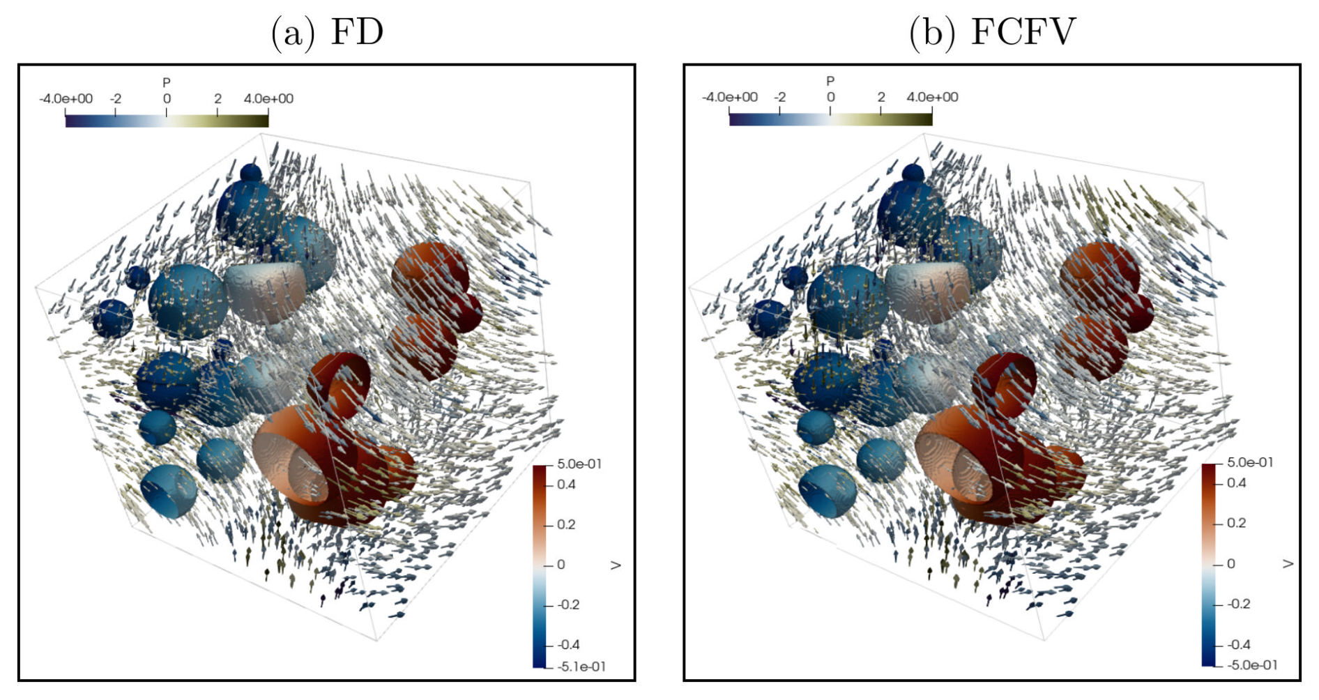
Figure 3 Example of multiple inclusion simulation result. Panels (a) and (b) shows the resulting flow field for the FD (320³ cells and the FCFV (256³ cells). The inclusions are coloured by the magnitude of the velocity vector (range: [0,0.75]). The black arrows indicate the velocity vectors.

Overall, the two methods exhibit a consistent and satisfactory qualitative agreement. Small differences between the two methods can be observed, particularly in regions where inclusions are in close proximity. These discrepancies stem from the different spatial resolution used for the FD and the FCFV methods, their different order of accuracy, and their different treatments of interfaces. A more detailed comparison of the FD and FCFV results is provided in the Appendix B. The stopping criteria of the PH/DR scheme was set to 10⁻⁶, the inner DR stropping criteria was set to 10⁻³, the penalty parameter was set to 15 times the mean of the viscosity field (γ=15〈η〉).

6.1.1 Scaling: problem size

The first test investigates the effect of problem size. To this end, we vary the model resolution by increasing the number of cells (N_x) uniformly along each dimension. The lowest resolution is 32³ cells, while the highest resolution is 320³ cells (131 Mdof) for the FD and 256³ cells (168 Mdof) for the FCFV.

The results show that for both the FD and the FCFV methods, 4 to 7 Powell–Hestenes iterations are required to reach convergence, regardless of the value of N_x. This number of Powell–Hestenes iterations appears to be largely insensitive to the problem size (Fig. 4a). In contrast, the total number of DR iterations accumulated throughout the solution process increases linearly with the problem size (Fig. 4b). This scaling behavior is consistent with that observed for the 1D Poisson problem discussed earlier (Sect. 4), and reflects the influence of the diagonal preconditioner. When normalized by the number of cells along one axis, the number of DR iterations required for convergence falls between 70 and 30 per N_x. The iteration count per N_x tends to decrease at higher resolutions, where the flow field is better resolved (Fig. 4c). The wall-time is reported as a function of the total number of degrees of freedom, N_dof. For both FD and FCFV, the observed scaling is approximately linear with respect to the problem size, which can be attributed to the combined effects of diagonal preconditioning and GPU parallelism (Fig. 4d). Interestingly, both FCFV and FD achieve comparable wall times for similar number of degrees of freedom and iterative tolerance ($\mathrm{1}\times {\mathrm{10}}^{-\mathrm{6}}$).

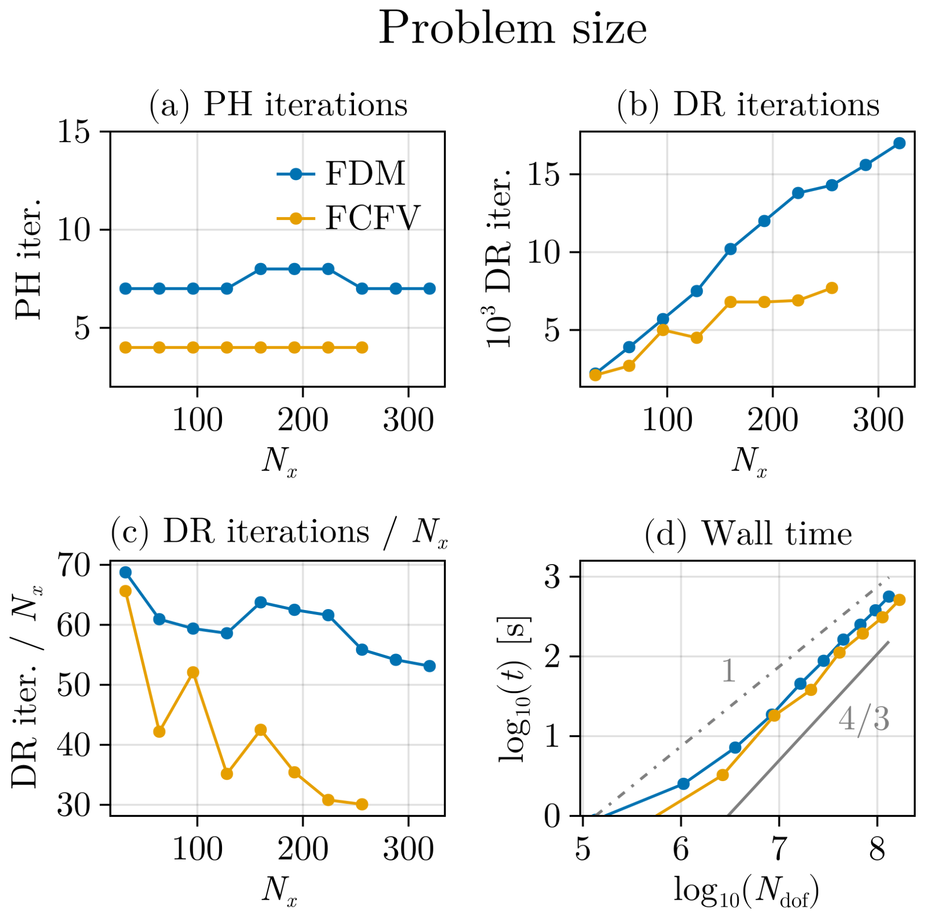
Figure 4 Influence of problem size on the convergence of the PH/DR flow solver for a viscosity contrast of 1×10⁴ using the FD and the FCFV methods. Panel (a) reports the total number of Powell–Hestenes iterations, (b) the total number of DR iterations for the entire solution procedure, (c) the number of DR iterations per grid point along one dimension, and (d) the wall-time.

6.1.2 Scaling: penalty factor

We further explore the influence of the penalty factor on the scaling of the PH/DR solver. In contrast to the previous tests, we vary the value of γ independently of the values of the viscosity field. We perform the computations for three different values of Δη.

The number of Powell–Hestenes iterations strongly depends on the magnitude of the penalty parameter γ. In particular, very small values of γ lead to a large number of Powell–Hestenes iterations that exceed 50 (Fig. 5a). This number decreases to fewer than 10 when γ>100, across all values of Δη. The total number of DR iterations is also higher for small values of γ, reflecting the increased number of Powell–Hestenes iterations required for convergence. However, excessively large values of γ also degrade convergence. Specifically, higher values of γ increase the spectral radius of the discrete velocity Schur complement, which in turn increases the number of DR iterations needed to reach convergence (Fig. 5b). An optimal range for γ is found between 10 and 1000, depending on the value of Δη. The wall-time exhibits a similar dependence on γ, closely following the behavior of the total number of DR iterations, with minimum values observed within the range 10–1000 (Fig. 5c).

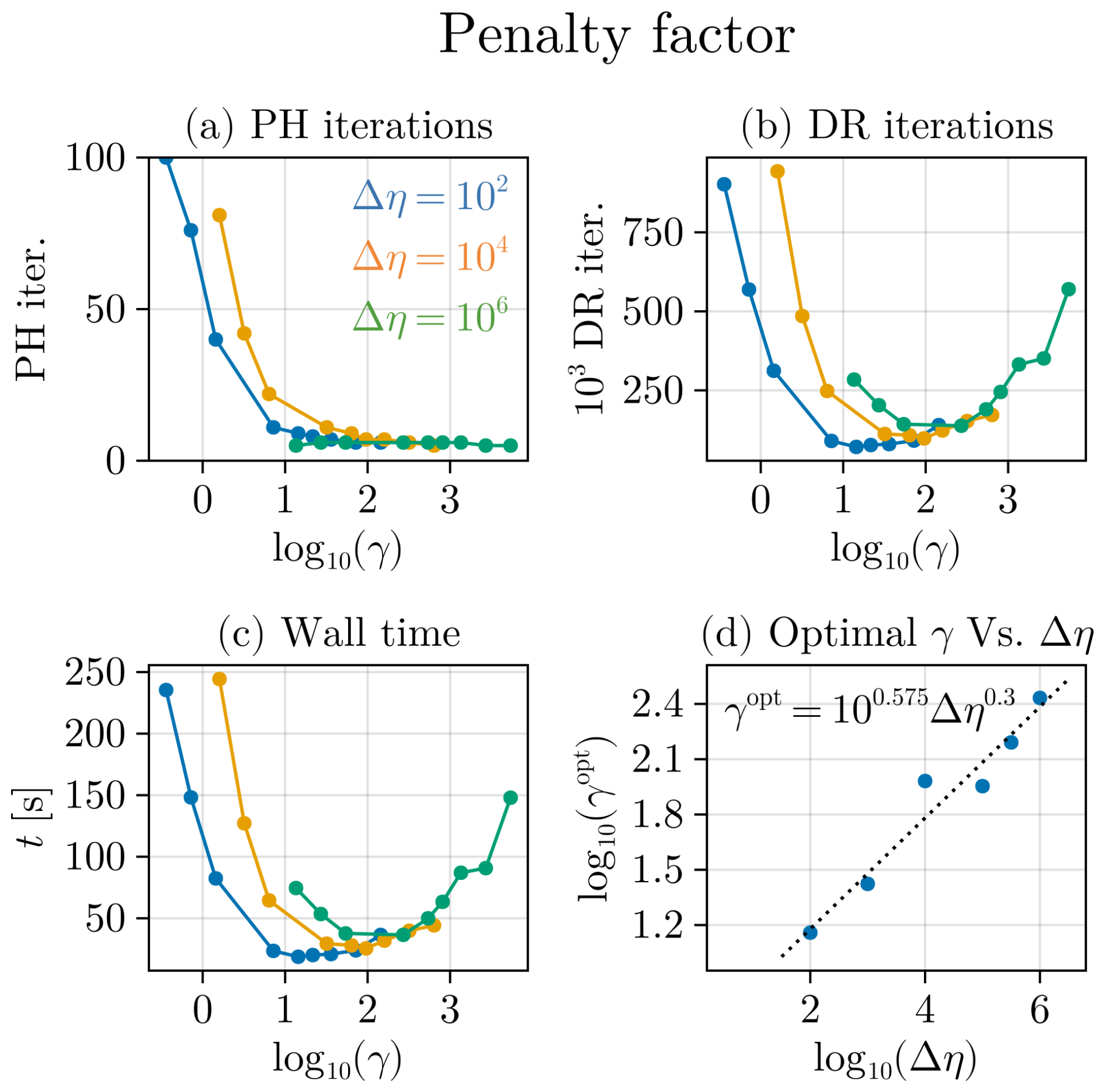
Figure 5 Influence of the penalty factor on the convergence of the PH/DR flow solver for a resolution of 128³ cells and 3 values of Δη. Panel (a) reports the total number of Powell–Hestenes iterations, (b) the total number of DR iteration for the entire solution procedure, (c) the wall time, and (d) the optimal value of γ as function of Δη

The magnitude of the penalty factor must be selected carefully to avoid an excessive number of iterations, which would degrade the wall-time. To guide this choice, we systematically varied the viscosity contrast and computed the optimal penalty value (γ^opt) for each corresponding Δη. The results reveal a linear relationship between γ^opt and Δη in log ₁₀–log ₁₀ space (Fig. 5d). This relationship allows for a least-squares fit with a slope of 0.3 and an intercept of 0.575. The resulting fit can be used to select an appropriate penalty parameter when varying the viscosity contrast. This particular scaling produces the best performance for the given model configuration; however, it should not be regarded as generally applicable to all cases. In most of the examples presented hereafter, we choose γ to be proportional to the mean of the viscosity field (γ∝〈η〉).

6.1.3 Scaling: viscosity contrast

We investigate the effect of viscosity contrast on the PH/DR solver by systematically varying it over a range spanning two to six orders of magnitude. As expected, increasing the viscosity contrast impacts the performance of the PH/DR solver.

The number of Powell–Hestenes iterations required for convergence ranges from 6 to 9 (Fig. 6a). The decrease in the number of Powell–Hestenes iterations with increasing Δη is attributed to the scaling of the penalty factor with the mean of the viscosity field. Therefore, higher values of Δη lead to higher values of γ, which in turn reduces the number of Powell–Hestenes iterations required for convergence. The total number of DR iterations scales approximately linearly with the viscosity contrast (Fig. 6b). Consequently, the wall-time also exhibits a linear dependency on the viscosity contrast (Fig. 6c).

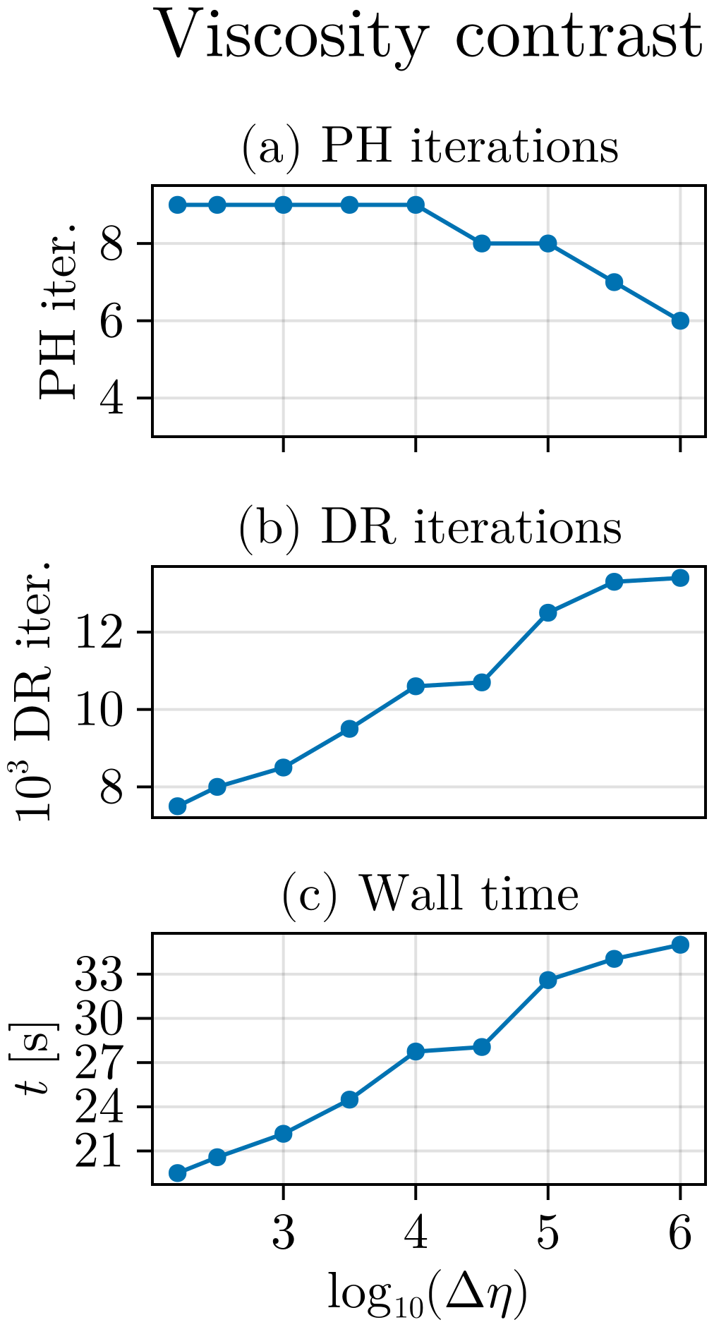
Figure 6 Influence of viscosity contrast on the convergence of the PH/DR flow solver for a resolution of 128³ cells and using γ^opt. Panel (a) reports the total number of Powell–Hestenes iterations, (b) the total number of DR iteration for the whole solution procedure, (c) the wall time.

6.1.4 Scaling: DR solve tolerance

Another important numerical parameter of the PH/DR procedure is the tolerance ϵ_DR selected to exit the inner DR iterations (ϵ_DR). We have systematically varied the value of ϵ_DR from 10⁻⁵ to 10^−0.5.

The magnitude of ϵ_DR has a significant impact on the number of Powell–Hestenes iterations. Small values lead to more accurate inner DR solves, resulting in fewer Powell–Hestenes iterations. In contrast, increasing ϵ_DR causes a quadratic increase in the number of Powell–Hestenes iterations (Fig. 7a). The trend differs for the total number of DR iterations. Very small and very large values of ϵ_DR lead to a high total iteration count, while a minimum is observed for ϵ_DR in the range 10⁻³ to 10⁻². High values of ϵ_DR result in inaccurate inner solves, increasing the number of Powell–Hestenes iterations. In contrast, very low values lead to over-solving of the inner system, unnecessarily increasing the total DR iterations (Fig. 7b). This behavior directly affects the wall-time, which can vary by up to a factor of 2 depending on the choice of ϵ_DR. Therefore, ϵ_DR must be carefully tuned to avoid these two limiting cases.

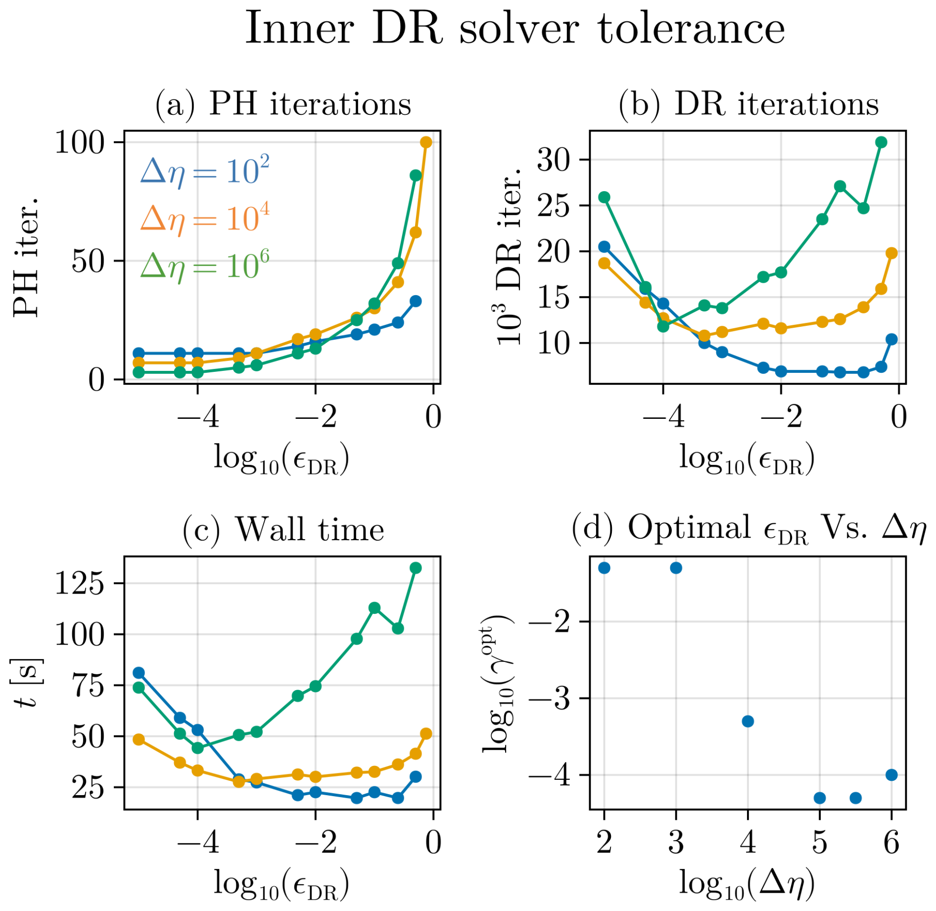
Figure 7 Influence of the inner DR solve tolerance on the convergence of the PH/DR flow solver for a resolution of 128³ cells and Δη=10⁴. Panel (a) reports the total number of Powell–Hestenes iterations, (b) the total number of DR iteration for the whole solution procedure, (c) the wall time. (d) Influence of the viscosity contrast.

7 Compressibility, multi-physics and nonlinear models

In this section, we show how the proposed PH/DR solution strategy can be further extended to solve steady mechanical problems that involve enriched physical models. These models are performed using the FD method, as the FCFV method still needs to be developed to tackle two-phase flow and nonlinear mechanical problems.

7.1 Compressible mechanical problem

Although the previous examples were performed in the incompressible limit, the PH/DR scheme can adequately handle compressible deformation or flow. Here, we show examples of compressible flow performed in 2D, using FD. The model configuration consists of a domain $\mathrm{\Omega }\in [\mathrm{0},\mathrm{1}]\times [\mathrm{0},\mathrm{1}]$ with a circular inclusion of radius 0.2 (Fig. 8a). The background viscosity is set to 1 and the inclusion viscosity is 100. Pure shear background deformation is applied at the boundaries. Compressibility is accounted for by including a bulk viscosity term:

$$\begin{array}{}\text{(28)}& {\displaystyle }\mathbf{\nabla }\cdot \mathit{\tau }-\mathbf{\nabla }P=\mathbf{0},\text{(29)}& {\displaystyle }\mathbf{\nabla }\cdot {\mathit{v}}^{\mathrm{s}}+{\displaystyle \frac{P}{{\mathit{\eta }}_{\mathrm{b}}}}=\mathrm{0}\end{array}$$

The degree of compressibility varies with the value of bulk viscosity (η_b). To solve this problem, one can use PH/DR, setting the penalty factor independently of the bulk viscosity. Here, we express the penalty factor as the quasi-harmonic average of a reference numerical bulk viscosity (γ_num=60〈η〉) and the physical bulk viscosity, γ_phys=η_b, so that $\mathit{\gamma }={\left(\mathrm{1}/{\mathit{\gamma }}_{\mathrm{phys}}+\mathrm{1}/{\mathit{\gamma }}_{\mathrm{num}}\right)}^{-\mathrm{1}}$. In this case, several Powell–Hestenes iterations will be needed to reach convergence. Alternatively, one can set the penalty factor to the bulk viscosity (γ=η_b). In that case, PH/DR becomes equivalent to a basic DR scheme and only one Powell–Hestenes iteration is needed to reach convergence. We observe that in the case of compressible problems (η_b=2.0, equivalent to a Poisson ratio of 0.286), the basic DR can be beneficial, leading to a lower number of iterations compared to PH/DR (Fig. 8b). The PH/DR solver exhibits a characteristic sawtooth convergence history that reflects the update of pressure at each Powell–Hestenes iteration (Fig. 8b). In contrast, in weakly compressible cases (${\mathit{\eta }}_{\mathrm{b}}=\mathrm{2}\times {\mathrm{10}}^{\mathrm{3}}$, equivalent to a Poisson ratio of 0.499), the PH/DR schemes outperform the standard DR iteration approach. In the context of geodynamic problems involving weakly compressible-to-incompressible materials, PH/DR is preferred.

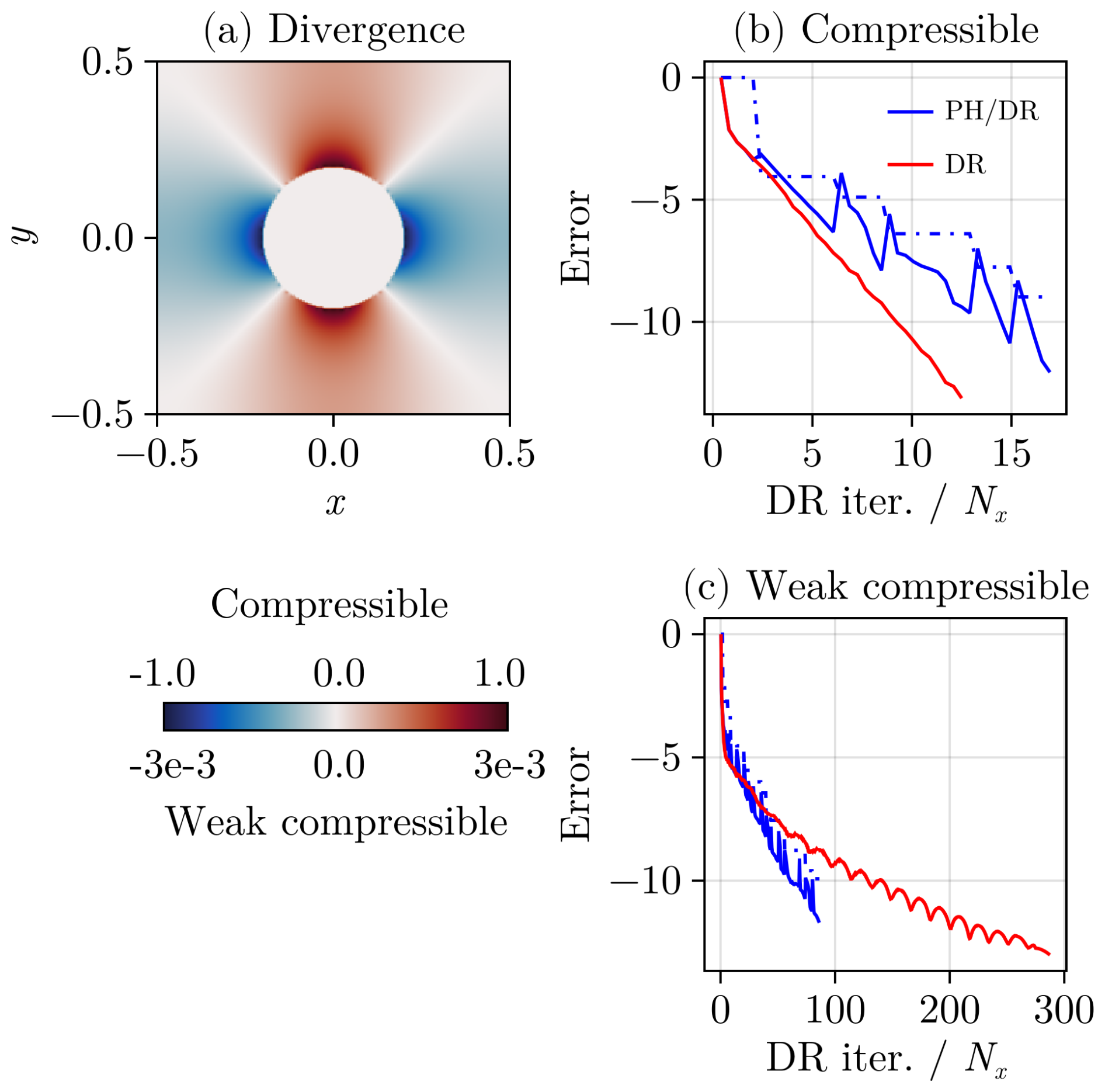
Figure 8 Example of compressible flow: pure shear deformation with viscosity heterogeneity. (a) Divergence field either compressible case (η_b=2) or weakly compressible case (${\mathit{\eta }}_{\mathrm{b}}=\mathrm{2}\times {\mathrm{10}}^{\mathrm{3}}$). Convergence history of DR and PH/DR for the (b) compressible and (c) weakly compressible case. For the PH/DR case, the solid line represents the velocity error norm and the dotted line corresponds to the pressure error norm. For the PH/DR case, iterations are summed over the Powell–Hestenes needed for converging the problem. In (a) and (b), x and y have arbitrary units.

7.2 Hydro-mechanical coupling

We further applied the PH/DR scheme to the solution of a coupled multi-physics problem. The equations governing deformation and fluid flow in a Darcy poro-viscous medium can be expressed following Yarushina and Podladchikov (2015):

$$\begin{array}{}\text{(30)}& {\displaystyle }\mathbf{\nabla }\cdot \stackrel{\mathrm{‾}}{\mathit{\tau }}-\mathbf{\nabla }\stackrel{\mathrm{‾}}{P}=\mathbf{0},\text{(31)}& {\displaystyle }\mathbf{\nabla }\cdot {\mathit{v}}^{\mathrm{s}}+{\displaystyle \frac{\stackrel{\mathrm{‾}}{P}-P^{\mathrm{f}}}{(\mathrm{1}-\mathit{\varphi }){\mathit{\eta }}_{\mathit{\varphi }}}}=\mathrm{0},\text{(32)}& {\displaystyle }\mathbf{\nabla }\cdot {\mathit{q}}^{\mathrm{D}}-{\displaystyle \frac{\stackrel{\mathrm{‾}}{P}-P^{\mathrm{f}}}{(\mathrm{1}-\mathit{\varphi }){\mathit{\eta }}_{\mathit{\varphi }}}}=\mathrm{0}.\end{array}$$

Here, the Darcy flux is expressed as ${\mathit{q}}^{\mathrm{D}}=-k^{\mathrm{f}}/{\mathit{\eta }}^{\mathrm{f}}\mathbf{\nabla }{P}^{\mathrm{f}}$. The overbar denotes phase-averaged quantities, ϕ is porosity, and the superscripts s and f indicate solid and fluid properties, respectively. k and η refer to permeability and viscosity. An elliptic equation for fluid pressure can be obtained by substituting the Darcy flux into Eq. (32).

The PH/DR scheme is extended by including fluid pressure updates within the inner DR iterations. The update parameters for fluid pressure are obtained from the automatic DR procedure described in Sect. 4. The pseudo-time steps and damping coefficients for velocity and fluid pressure are determined independently, with each variable assigned its own value. As in previous examples, the total pressure is updated at each Powell–Hestenes iteration.

The test case we consider uses a configuration similar to that in the previous example (Sect. 7.1). The shear viscosity of the inclusion is assigned a value 100 times greater than that of the matrix, while the bulk viscosity is taken as twice the shear viscosity. In addition, the background porosity is set to $\mathrm{1}\times {\mathrm{10}}^{-\mathrm{3}}$, and the fluid permeability-viscosity ratio $\left(k^{\mathrm{f}}/{\mathit{\eta }}^{\mathrm{f}}\right)$ is set to $\mathrm{1}\times {\mathrm{10}}^{-\mathrm{3}}$. The penalty factor is defined as

$$\mathit{\gamma }={\left({\displaystyle \frac{\mathrm{1}}{{\mathit{\gamma }}_{\mathrm{phys}}}}+{\displaystyle \frac{\mathrm{1}}{{\mathit{\gamma }}_{\mathrm{num}}}}\right)}^{-\mathrm{1}},$$

where ${\mathit{\gamma }}_{\mathrm{phys}}=(\mathrm{1}-\mathit{\varphi }){\mathit{\eta }}_{\mathit{\varphi }}$ and γ_num=5〈η^s〉.

Figure 9 shows examples of solution fields and the scaling properties of the PH/DR scheme. We compute the two-phase flow problem with a resolution varying from 31² to 992² cells and apply a tolerance of 10⁻⁷. For the chosen parameters, pronounced differences are observed between the total and fluid pressure fields (Fig. 9a, b). The total pressure field is sharply defined and zero inside the stiff inclusion, in contrast to the fluid pressure field, which is smoother and diffuses within the inclusion. We observe the characteristic sawtooth convergence history for both momentum and fluid continuity (Fig. 9c).

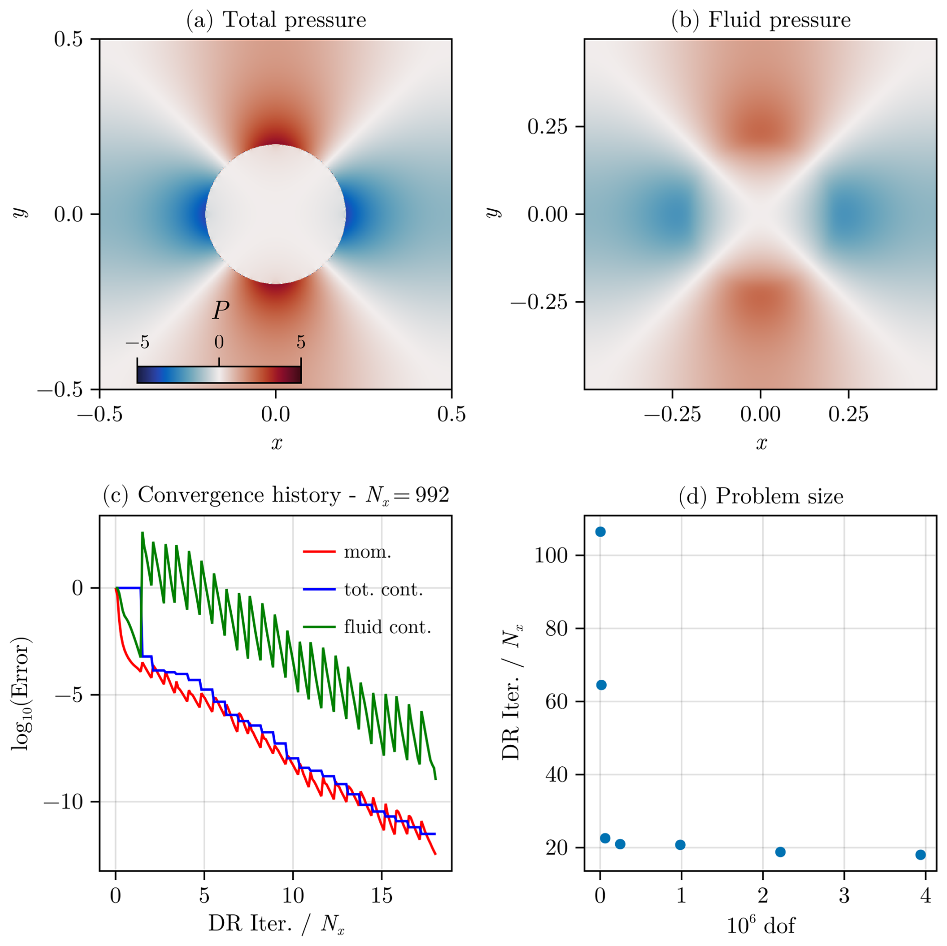
Figure 9 Poro-viscous hydro-mechanical simulation. (a) Total pressure field. (b) Fluid pressure field. (c) Convergence history for a resolution of 992². (d) Scaling of iterations relative to the problem size. In (a) and (b), x and y have arbitrary units.

We find that low-resolution models require a relatively high number of iterations (Fig. 9d). Nevertheless, the number of DR iterations per N_x drops to a stable low value (approximately 20) for resolutions greater than 100² cells. This indicates a linear dependence of the number of iterations on the problem size, which is consistent with the behavior documented in the previous examples.

7.3 Visco-elasto-viscoplasticity

In this example, we show how nonlinear material properties can be incorporated into the PH/DR solution strategy, considering the case of non-associated plasticity. With such nonlinear problems, parameters such as the effective viscosity vary throughout the nonlinear solution procedure, which directly affects the eigenvalues of the discrete operator. It is thus important to reevaluate the maximum pseudo-time step (Eq. 18) during the iterations to ensure stability of the procedure. Here, we reevaluate the pseudo-time step every 100 iterations by applying the Gershgorin circle theorem (Eq. 21).

We adopt a single-phase formulation and apply a visco-elasto-viscoplastic material model (de Borst and Duretz, 2020). An additive decomposition of the deviatoric strain rate and the divergence rate is assumed:

$$\begin{array}{}\text{(33)}& {\displaystyle }\dot{\mathit{\epsilon }}={\dot{\mathit{\epsilon }}}^{\mathrm{v}}+{\dot{\mathit{\epsilon }}}^{\mathrm{e}}+{\dot{\mathit{\epsilon }}}^{\mathrm{p}}\text{(34)}& {\displaystyle }\mathbf{\nabla }\cdot \mathit{v}={\left(\mathbf{\nabla }\cdot \mathit{v}\right)}^{\mathrm{e}}+{\left(\mathbf{\nabla }\cdot \mathit{v}\right)}^{\mathrm{p}}\end{array}$$

where the superscripts v, e, and p correspond to the viscous, elastic, and plastic components, respectively.

The viscoplastic Drucker–Prager yield and potential functions are defined as:

$$\begin{array}{}\text{(35)}& {\displaystyle }f={\mathit{\tau }}_{\mathrm{II}}-P\sin \mathrm{\Phi }-C\cos \mathrm{\Phi }-\dot{\mathit{\lambda }}{\mathit{\eta }}^{\mathrm{vp}}\text{(36)}& {\displaystyle }q={\mathit{\tau }}_{\mathrm{II}}-P\sin \mathrm{\Psi }\end{array}$$

where τ_II, C, Φ, Ψ, and η^vp denote the second deviatoric stress invariant, the cohesion, the friction angle, the dilatancy angle, and the viscoplastic viscosity, respectively.

The model domain is $\mathrm{\Omega }\in [\mathrm{0},\mathrm{2}]\times [\mathrm{0},\mathrm{1}]$ km² and contains a circular inclusion of radius $\mathrm{1}\times {\mathrm{10}}^{-\mathrm{1}}$ km (Fig. 10a). A pure shear loading rate of $-\mathrm{1}\times {\mathrm{10}}^{-\mathrm{15}}$ s⁻¹ is applied, inducing horizontal extension. The inclusion has a low viscosity (1×10¹⁰ Pa s), while the surrounding matrix is effectively elasto-plastic (1×10²³ Pa s). Both shear and bulk moduli are set to 3×10¹⁰ Pa. The cohesion is set to 50 MPa, the friction and dilatancy angles are set to 35 and 5°, respectively, and the viscoplastic viscosity is 2×10²⁰ Pa s. The simulation proceeds over 50 time steps, each of size $\mathrm{\Delta }t=\mathrm{4}\times {\mathrm{10}}^{\mathrm{10}}$ s.

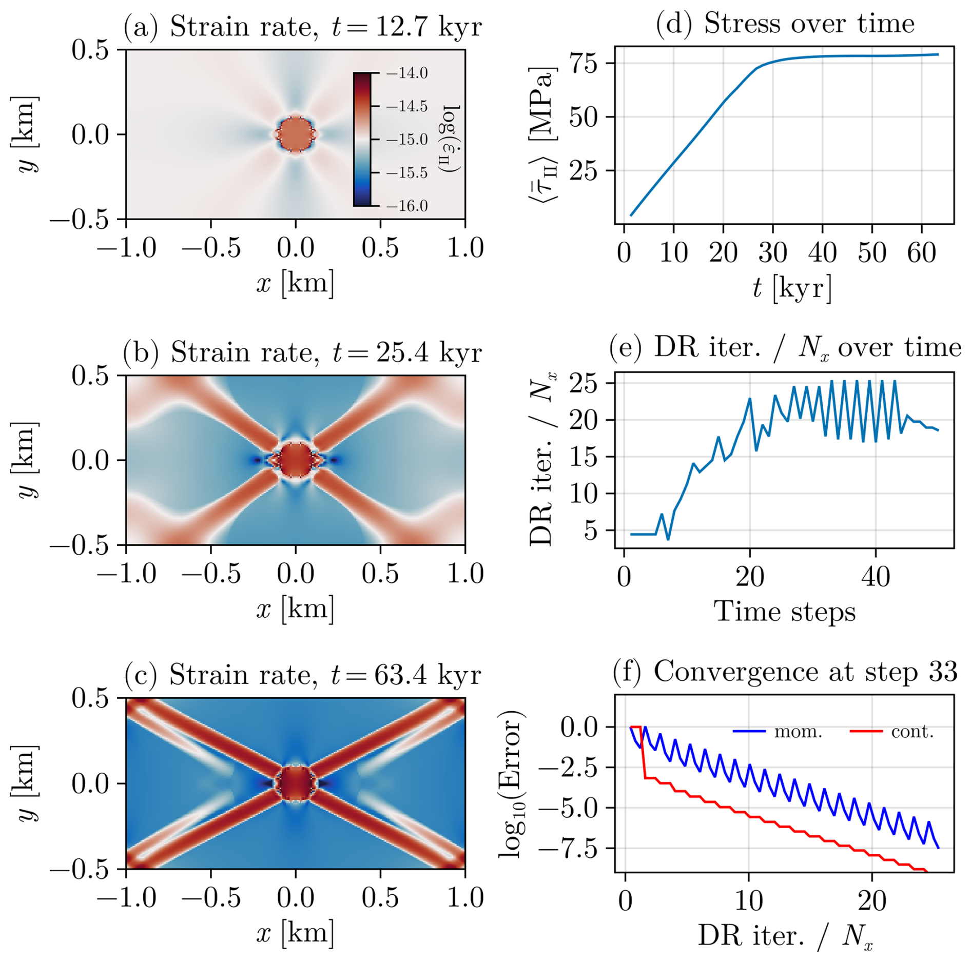
Figure 10 Visco-Elasto-Viscoplastic shear banding. (a, b, c) Model evolution (strain rate field). (d) Evolution of the mean stress. (e) Number of iteration per grid point in x over simulation time. (f) Convergence history for the most demanding time step.

The temporal evolution of the second invariant of the deviatoric strain rate is shown in Fig. 10a, b, and c, while the evolution of the mean stress is shown in Fig. 10d. The model undergoes an initial phase of elastic loading (Fig. 10a), after which shear banding initiates, propagates (Fig. 10b), and reflects off the domain boundaries (Fig. 10c). As a result, stress is limited after 30 kyr and undergoes minor fluctuations witnessing underlying structural softening (Fig. 10d). With a relative tolerance of $\mathrm{1}\times {\mathrm{10}}^{-\mathrm{6}}$, the number of iterations per N_x varies between 5 and 25 (Fig. 10e). Low iteration counts correspond to linear-elastic steps, while higher counts occur during nonlinear steps involving significant changes in the solution pattern (e.g. reflections). The convergence history for the most challenging step is shown in Fig. 10f, where the typical sawtooth convergence pattern of the PH/DR is also observed.

Overall, the model converges reliably without the need for manual tuning of numerical parameters throughout the simulation.

7.4 Practical Performance of the PH/DR Method

In this section, we investigate the benefits of the proposed PH/DR method for solving two practical geodynamic problems. The main benefit of the PH/DR method over the APT approach is its ability to automatically adapt to transient changes in solution patterns, caused by variation of the model geometry or by the emergence of internal features. The PH/DR approach can therefore determine parameters that ensure convergence while also significantly reducing the overall wall time. The results presented below are intended to be indicative. In principle, the APT method could deliver results that are at least as good as those of the PH/DR method. However, this would require manually tuning the iteration parameters at every time step, which is not a desirable task. Several simulations were performed using the open-source code JustRelax.jl (de Montserrat et al., 2026), which features both the PH/DR solver and the Accelerated Pseudo-Transient (APT) method (Räss et al., 2022).

The first model is a simplified subduction setup based on the configuration of Schmeling et al. (2008). Simulations were performed over a model duration of 25 Myr, after which the slab tip reaches a depth of approximately 500 km (Fig. 11). We observe that the use of the PH/DR scheme significantly reduces cumulative wall time compared to the APT method (Fig. 11a). The number of iterations per grid point in one dimension is also well behaved, fluctuating around 20 iterations per grid point. For the same tolerance, the APT scheme requires about 200 iterations per grid point and exhibits larger fluctuations (Fig. 11b). Overall, both approaches converge at each iteration and yield similar results (Fig. 11c, d).

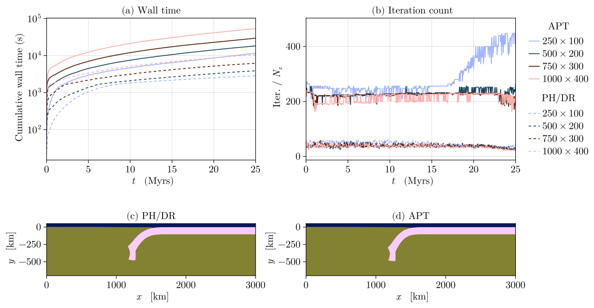
Figure 11 (a) Cumulative wall times over 25 Myr of model simulation steps using both PH/DR and APT methods at various resolutions. (b) Iterations per time step for the two methods. (c) Map of material phases at 25 Myr using the PH/DR method. The mantle is green, the slab is pink and the sticky air is blue. (d) Same as (c) for the APT method.

The second model is a crustal-scale shear banding setup, which features a visco-elasto-viscoplastic rheology and temperature-dependent creep laws. The reader is referred to Duretz et al. (2020) for the detailed model configuration and material parameters. The simulations are run for 100 time steps, in which the solution pattern evolves significantly in response to shear banding and frictional viscoplasticity. The results presented in Fig. 12 show the cumulative wall time and the number of iterations over 100 time steps for various model resolutions. Models performed with the PH/DR scheme consistently result in 2 to 12 times shorter wall times (Fig. 12a). Unlike APT models, simulations using the PH/DR method provide a reliable and well-defined range of iterations per time step. Nevertheless, the overall shear banding patterns are similar (Fig. 12c, d). The minor differences may be attributed to the fact that APT models could not reach convergence at every time step.

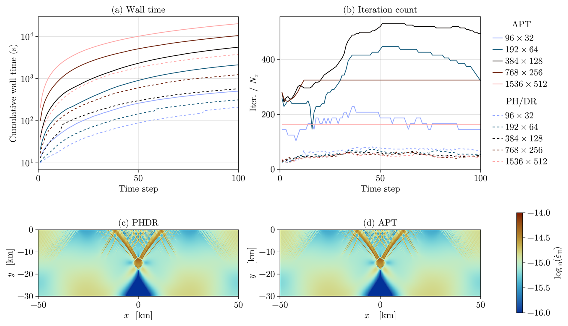
Figure 12 (a) Cumulative wall times over 100 time steps for both PH/DR and APT methods at various resolutions. (b) Iterations per time step for the two methods. The number of pseudo-transient iterations per time step was capped at 250×10³; as a result, some APT simulations did not reach the convergence criteria (relative tolerance of $\mathrm{1}\times {\mathrm{10}}^{-\mathrm{6}}$). (c) Map of the second deviatoric strain rate invariant at time step 100 (1 Myr) obtained with the PH/DR method. (d) Same as (c) for the APT method.

8 Discussion

Our study presents a quantitative assessment of the performance of the DR method, extends it to incompressible flow problems through a Powell–Hestenes strategy, and demonstrates its applicability to nonlinear and multiphysics problems.

The efficiency of pseudo-transient (PT) solvers relies on a careful selection of iterative parameters (see Appendix C). The proposed DR and PHDR solvers are not expected to outperform standard PT solvers with optimally chosen parameters. However, the DR-based methods introduced here are designed to automatically determine these iterative parameters. This automated selection introduces only a minor computational overhead and has a negligible impact on the convergence history compared to an optimally tuned PT solver (see Appendix D). In practice, DR-based schemes can offer substantial advantages over standard pseudo-transient solvers that do not feature automatic tuning of iteration parameters.

Unlike multigrid methods, DR-based approaches exhibit a total iteration count that increases linearly with problem size (see Figs. 2 and 4b). Although this behavior may appear disadvantageous, the DR methods are straightforward to parallelize and require only a few global communication steps. In all the examples presented, global communication operations (e.g., norms and inner products) and iterative parameter updates were performed every 100 DR iterations. This makes DR-based methods particularly suitable for GPU parallelism.

In particular, we show that, when using a single GPU, the wall time for three-dimensional incompressible and heterogeneous Stokes problems scales quasi-linearly with problem size (Fig. 4d). This property is attractive for large-scale 3D geodynamic simulations and makes DR-based algorithms competitive with legacy multigrid-based solvers.

Furthermore, DR-based solvers can be naturally extended to multi-GPU parallelism. Computational frameworks such as ImplicitGlobalGrid.jl (Omlin et al., 2022) provide efficient communication scheduling schemes, enabling near-ideal scaling behavior in modern computing clusters (Räss et al., 2022). In the future, several improvements may be envisaged, in particular regarding preconditioning. To our knowledge, Jacobi preconditioning is known to be relatively inefficient in comparison to other preconditioners (e.g. incomplete Cholesky). Nevertheless, the application of Jacobi is fully parallel, and thus efficiently implemented on GPUs. Recently, iterative implementations of incomplete LU and Cholesky preconditioners have been introduced (Anzt et al., 2016; Chow et al., 2018). Although these methods are fully parallel, achieving effective preconditioning requires accurate application of the LU/Cholesky operators, often necessitating many iterations. Whether such an approach would offer benefits within the framework of DR solvers remains to be established. Multigrid preconditioning represents another possible avenue. In principle, it could maintain a constant iteration count as the resolution increases. However, its implementation requires hierarchical data structures and coarse-grid solvers on GPUs, and it remains uncertain whether this added complexity would yield tangible reductions in wall time or enhance the already quasi-linear wall time scaling.

DR solvers are traditionally used in conjunction with the Finite Element Method (FEM) (e.g. Oakley and Knight, 1995; Joldes et al., 2011). Here, we have shown that such solvers can also be applied to finite difference methods, as well as finite volume or low-order discontinuous Galerkin methods. In practice, efficient implementation is facilitated by the structured nature of these problems, which allows information from neighboring cells to be easily gathered for stencil evaluations. Extending DR solvers to unstructured FEM or FCFV discretizations in the context of GPU computing requires specialized algorithms to improve memory access (e.g. Fu et al., 2014; Kiran et al., 2019). The combination of these approaches with DR solvers may provide an alternative to traditionally employed solvers, a possibility that remains to be explored.

The relatively low algorithmic complexity of DR methods makes them particularly attractive for solving nonlinear and multiphysics coupled problems. While we have focused on basic hydro-mechanical and linear plasticity models, future implementations could naturally extend these solvers to include thermal or chemical couplings.

9 Conclusions

In this contribution, we have employed DR-based techniques to develop robust and high-performance solvers for geodynamic problems. These solvers incorporate automatic tuning of iterative parameters, including pseudo-time steps and damping coefficients based on estimates of the spectral bounds of the discrete operators.

The approach was applied to problems discretized on structured grids using both finite-difference (FD) and face-centered finite-volume/discontinuous Galerkin (FCFV) methods. To handle incompressible deformations, DR-based solvers were combined with Powell–Hestenes iterations, enabling the successful solution of heterogeneous Stokes problems.

When implemented on GPU accelerators, the solvers exhibit a quasi-linear scaling of solution time with problem size, demonstrating excellent computational efficiency. Moreover, the method can be trivially extended to handle compressible flow, multiphase flow, and nonlinear constitutive laws.

This flexibility stems from the algorithmic simplicity of the DR-based methods, which makes them particularly well-suited for large-scale geoscientific simulations and opens new paths for exploring complex coupled physical processes.

Appendix A: Three-dimensional multiple inclusion problem

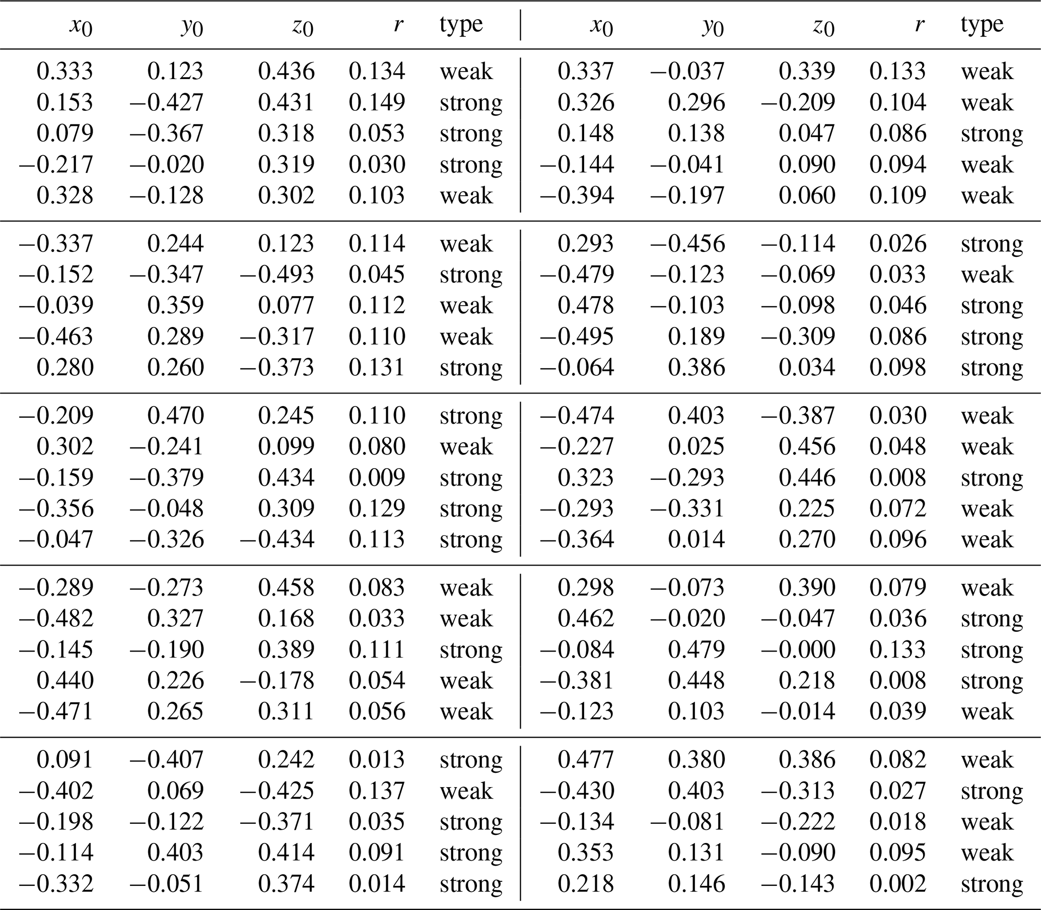
The position and type of inclusion used in the example in the main text are provided in the following table (Table A1). The extent of the model domain and the viscosity contrast are detailed in the main text.

Table A1 Tabulated values of x₀, y₀, z₀, r, and type (weak/strong). Each block of 5 rows is shown side by side.

Appendix B: Two-dimensional heterogeneous Stokes flow with FD and FCFV

To verify our implementation of PH/DR iterative solvers, the results were compared against solutions obtained using direct solvers. This verification could only be conducted in 2D due to the prohibitive computational cost of direct solvers in 3D. Both FD and FCFV models were executed using configurations analogous to the 3D setups. The inclusion positions are given in the table below (Table B1): weak inclusions have a viscosity of $\mathrm{1}\times {\mathrm{10}}^{-\mathrm{3}}$, while strong inclusions have a viscosity of 1000. No smoothing of the viscosity contrast was applied. A background pure shear rate and free-slip boundary conditions were imposed on the box boundaries.

FD models solved with a direct solver follow the approach of Räss et al. (2017), whereas the FCFV direct-solver implementation is based on Sevilla and Duretz (2023). All simulations were performed on meshes of 128² cells. The resulting pressure fields are shown in Fig. B1.

For both discretizations, good agreement is obtained between models solved iteratively and those solved directly, demonstrating that the FD and FCFV implementations are consistent with previous studies. In addition, this comparison highlights differences between the two schemes: while the FD approach exhibits spurious oscillations at sharp viscosity contrasts, the FCFV method yields a smoother pressure field. It should be noted that the mesh used in the FCFV simulations is similar to that of the FD models and does not explicitly capture the material interface through traction continuity enforcement.

Table B1 Tabulated values of x₀, y₀, r, and type (weak/strong). Each block of 5 rows is shown side by side.

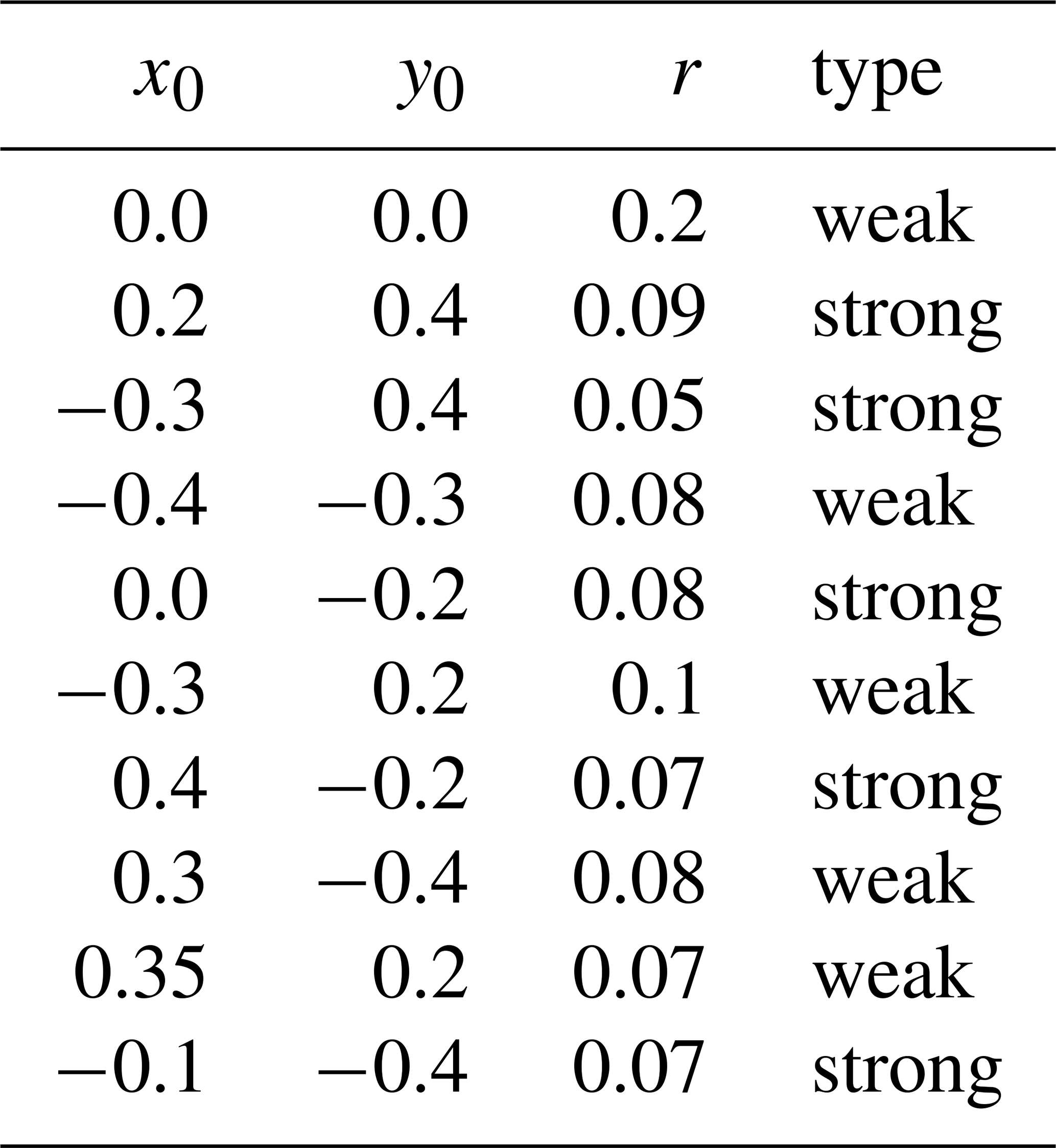
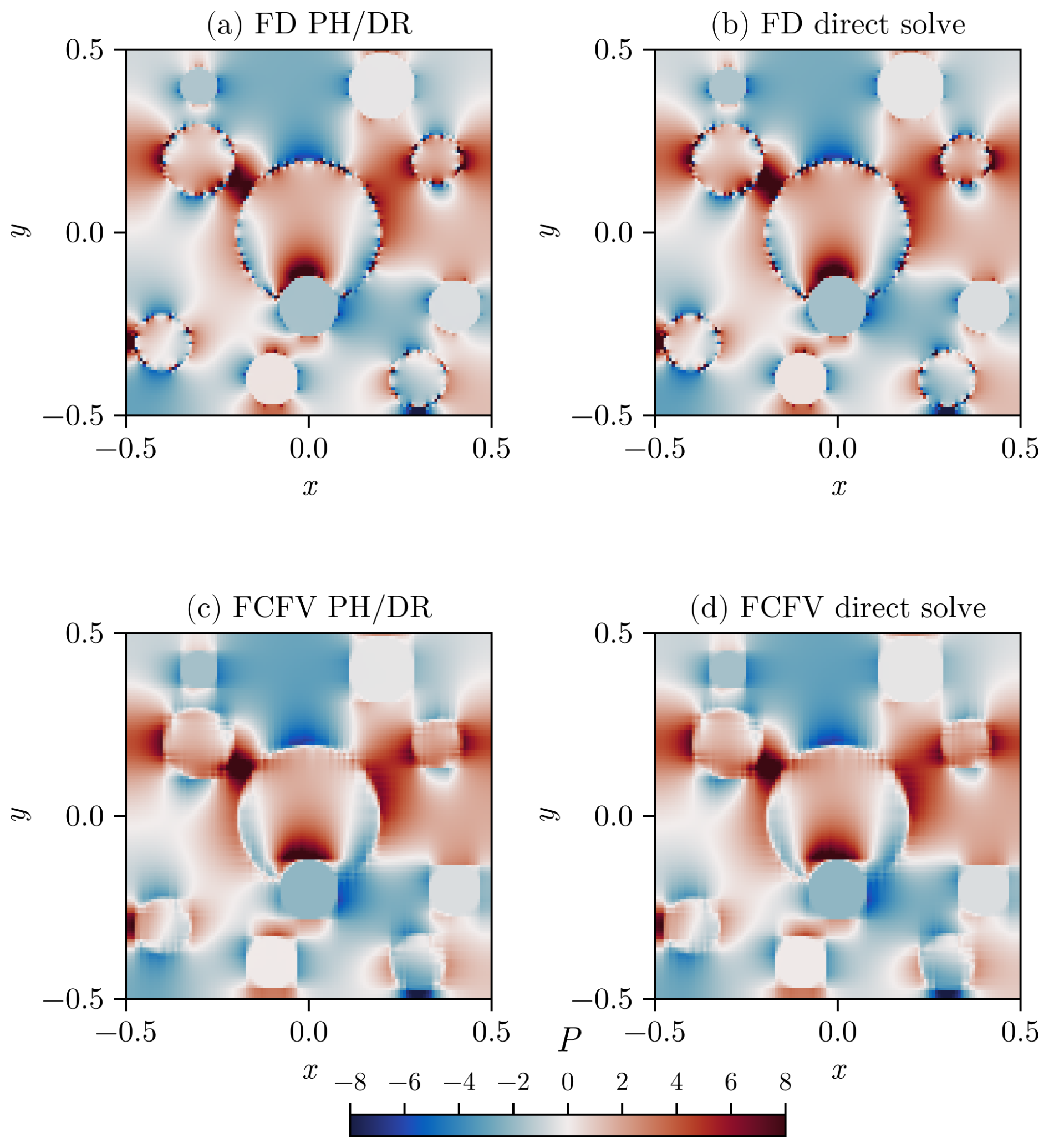
Figure B1 (a) Pressure field obtained with FD using a PH/DR scheme. (b) Pressure field obtained with a direct solution scheme. (c) Pressure field obtained with FCFV using a PH/DR scheme. (d) Pressure field obtained with FCFV using a direct solution scheme. In all panels, x and y have arbitrary units.

Appendix C: Comparison with the pseudo-transient formulation

The DR and PH/DR schemes are formulated in a manner similar to pseudo-transient (PT) solvers. The solution fields are updated iteratively, with update steps determined through stability analysis to ensure stable integration in pseudo-time. Most importantly, damping is applied, which effectively modifies the form of the equation to be integrated in pseudo-time, resulting in a second-order integration scheme following Frankel (1950). The pseudo-time step and damping parameters constitute the two numerical parameters that control the convergence behavior.

Optimal values for these parameters can be derived analytically (e.g. Räss et al., 2022). However, they depend on the spectral properties of the discrete operator Papadrakakis (1981); Oakley and Knight (1995). Consequently, determining iteration parameters a priori that remain optimal throughout simulations involving evolving geometry or time-dependent material properties is highly challenging. This may result in degraded convergence, stagnation, or even divergence.

The DR and PH/DR schemes address this difficulty by estimating spectral bounds and adjusting the iteration parameters accordingly. In practice, the main additional components are:

1. a routine to estimate the maximum eigenvalue (Gershgorin analysis),

2. a routine to approximate the minimum eigenvalue (Rayleigh quotient), and

3. a recalculation of the iteration parameters based on these estimates.

In addition, the PH/DR scheme features an outer loop for pressure updates. During the velocity update cycles, the pressure is held fixed. At the end of each such cycle, the pressure is updated using a numerical bulk viscosity and the continuity residual, following the classical Powell–Hestenes approach. The pressure is thus updated less frequently than the velocity, which constitutes a key difference from the pseudo-transient approach presented in Räss et al. (2022).

Appendix D: Comparison with the pseudo-transient formulation and the results of Räss et al. (2022)

We employed the PT solvers developed by Räss et al. (2022) to assess the relative performance of the PH/DR solver, using the single-inclusion benchmark configuration. The inclusion has a viscosity of $\mathrm{1}\times {\mathrm{10}}^{-\mathrm{3}}$, while the surrounding matrix has a viscosity of 1. A smoothing of the viscosity contrast similar to that used in Räss et al. (2022) was applied. Both the PT and PH/DR models were run to the same relative tolerance of $\mathrm{1}\times {\mathrm{10}}^{-\mathrm{6}}$. The resulting model fields are shown in Fig. D1.

The PT models of Räss et al. (2022) were computed using optimally tuned iterative parameters and thus represent the best possible performance bound. The present results demonstrate that the additional computational cost associated with the automatic parameter selection inherent to the PH/DR scheme is very small. Both methods converge in fewer than 20 iterations per grid point for this model configuration. Because pressure updates are less frequent than velocity updates, the convergence of the pressure residual does not closely track that of the momentum residuals.

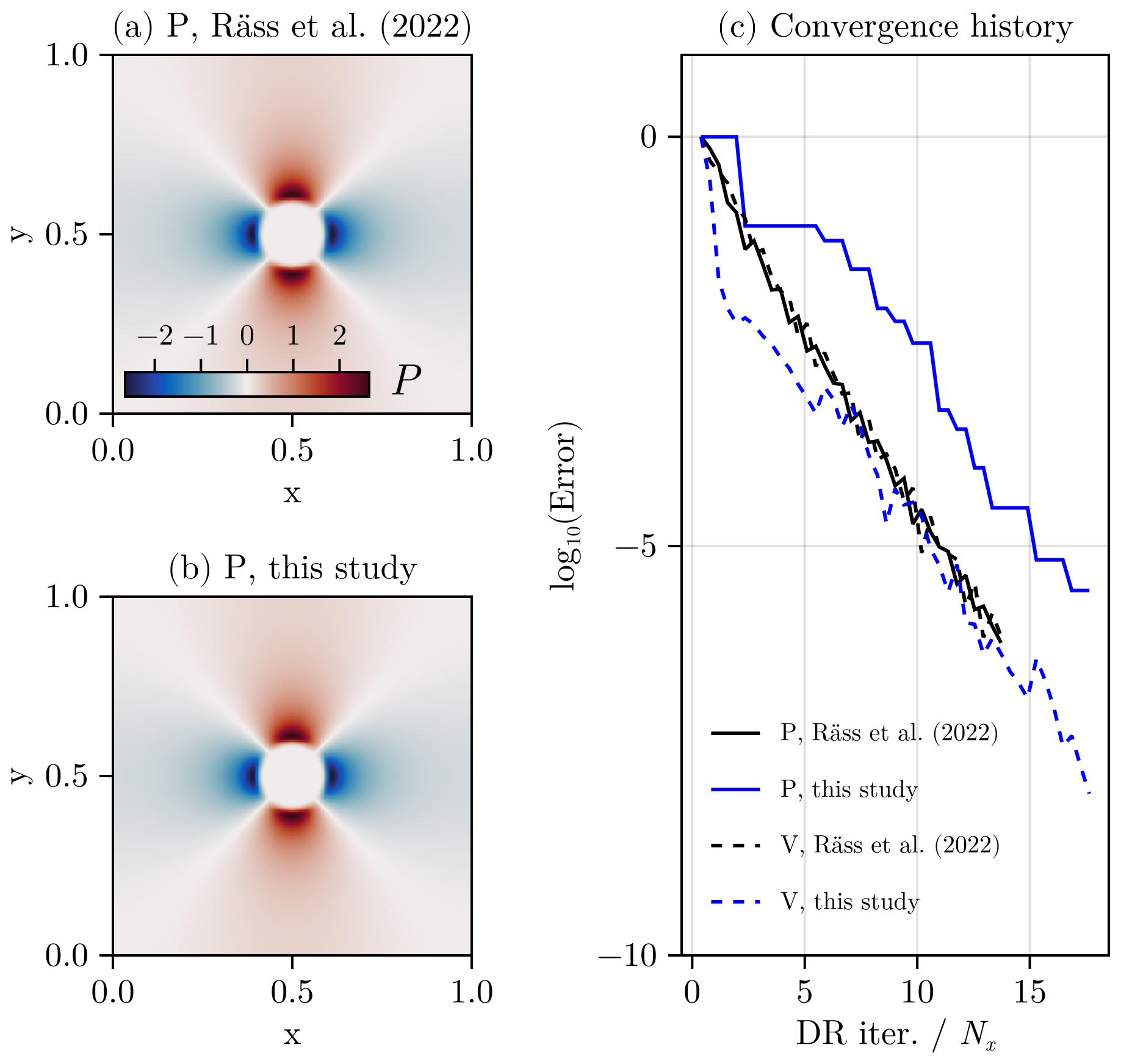
Figure D1 (a) Pressure field obtained by Räss et al. (2022). (b) Pressure field obtained in this study. (c) Convergence of momentum and continuity residuals. In (a) and (b), x and y have arbitrary units.