G&M3D 1.0: an interactive framework for 3D model construction and forward calculation of potential fields

Building source models and performing forward calculations are fundamental for processing, analyzing, and interpreting geophysical data. However, open-source tools that allow for both the flexible and interactive construction of source models and potential-field forward calculations are rare. To address this gap, we develop a new Qt-based software called G&M3D 1.0 (Gravity and Magnetic 3D modelling), which supports interactive three-dimensional (3D) model construction and provides accurate and efficient forward modelling. G&M3D 1.0 features two core functionalities: (1) constructing 3D gravity and magnetic source models and (2) calculating and visualizing their gravity/magnetic fields, as well as their gradient fields. In the 3D Modelling Module, user-defined anomalous bodies are internally discretized into assemblies of rectangular prisms for forward calculation. Based on this prism-based representation, users can conveniently construct regular bodies, such as spheres, cuboids, cylinders, ellipsoids and prismoids, and assign density contrast or magnetic parameters to them. Complex structures can be represented using the Irregular (Layer-Building) tool, which is especially suitable for stratigraphic or faulted formations. In addition, the Forward-Modelling Module allows for the rapid calculation, visualization, and saving of gravity anomalies, gravity gradients, total magnetic intensity, and magnetic gradients generated by the created 3D sources. To enhance computational efficiency, the software employs a 2D discrete convolution algorithm for the gravity and magnetic forward calculations. G&M3D 1.0 offers several significant advantages, including open-source accessibility, flexible interactive operations, an intuitive 3D modelling interface, efficient forward computation, and excellent file portability. As a demonstration of its capabilities, we use G&M3D 1.0 for forward gravity modelling over a salt dome at Vinton Dome in southern Louisiana, U.S., validating its accuracy and practicality.

1 Introduction

Compared with more logistically demanding methods, such as seismic reflection surveys and electrical surveys requiring dense electrode deployment, gravity and magnetic surveys generally offer simpler field procedures, lower acquisition costs, and greater efficiency for large-area data collection. Building forward source models and conducting forward calculations are fundamental to the processing, analysis, and interpretation of gravity and magnetic data (Blakely, 1996). Although several open-source tools already exist, few available tools combine interactive 3D body construction, gravity and magnetic forward calculation, and result visualization within a standalone graphical user interface (GUI).

To estimate the gravitational or magnetic effects generated by anomalous masses, geophysicists often represent complex subsurface volumes or geological bodies as a combination of idealized sources with simple shapes (Blakely, 1996; Hinze et al., 2013). These shapes include spheres, cylinders, vertical laminas, horizontal laminas, prisms, and polyhedra. Most of these idealized sources can be easily integrated over the volume and evaluated in closed analytical forms. Among these simple cells, the rectangular prism is particularly favoured for forward modelling and is also widely used in inversion studies, as it provides a straightforward way to approximate complicated anomalous sources and represents the total underground volume without gaps (Caratori Tontini et al., 2009; Li and Chouteau, 1998; Zhao et al., 2018).

Numerous early scholars have contributed to the closed formulas for gravity and magnetic anomalies caused by rectangular prisms (Bhattacharyya, 1964; Bhattacharyya and Navolio, 1976; Li and Chouteau, 1998; Nagy, 1966; Nagy et al., 2000; Okabe, 1979; Plouff, 1976). For example, Bhattacharyya (1964) presented formulas for the magnetic anomalies resulting from prism-shaped bodies with arbitrary polarization. Nagy (1966) derived a closed expression to calculate the gravitational attraction of a rectangular prism. Bhattacharyya and Navolio (1976) provided spectral expressions for the gravity and magnetic anomalies arising from irregular three-dimensional (3D) sources by combining prisms. Later, Guo et al. (2004) introduced a new singularity-free calculation formula for the forward modelling of the magnetic field produced by a rectangular prism. Additionally, Luo and Yao (2007) optimized the theoretical magnetic calculation formula to enhance its computational efficiency.

A fine subdivision is often required to approximate anomalous bodies more precisely. However, when the subspace is finely subdivided, the repeated cumulative calculations can make the forward analysis time-consuming. To improve calculation efficiency, various algorithms have been developed for forward calculations of gravity and magnetic anomalies. For instance, Wu and Tian (2014) proposed a Gauss-fast Fourier transform (FFT) method for calculating potential fields in the Fourier domain. Zhang and Wong (2015) established a block-Toeplitz-Toeplitz-block (BTTB) structure using a discrete multi-layer model, then embedded the BTTB matrix into a block-cyclic-cyclic-block (BCCB) matrix by applying FFT in forward calculations. Additionally, Chen and Liu (2019) optimized the computation of the weight coefficient matrix and applied a 2D discrete convolution algorithm through block circulant extension (referred to as the BCE method) to calculate the gravity anomaly in the spatial domain. This method was later extended to calculate magnetic anomalies on undulating terrain (Qiang et al., 2019). Subsequently, Hogue et al. (2020) developed an open-source MATLAB code for evaluating gravity and magnetic kernels based on the BCE method. Recently, Yuan et al. (2022) advanced the BCE algorithm for magnetic forward modelling.

Significant progress has been made in the forward calculation of the potential fields; however, constructing 3D anomalous models for algorithm testing or generating synthetic models for inversion studies remains complex and non-intuitive, especially when creating intricate, irregular sources (Jessell et al., 2021). To address these needs, various software packages have been developed for the computational synthesis of geological models and geophysical simulations (Bauville and Baumann, 2019; Cockett et al., 2015; de la Varga et al., 2019; Hassanzadeh et al., 2022; Pirot et al., 2022; Ulug and Karslıoglu, 2022; Wellmann et al., 2016). For example, SimPEG provides a flexible open-source framework for geophysical simulation (Cockett et al., 2015), while geomIO supports geometrical model construction for numerical simulations (Bauville and Baumann, 2019). Additionally, Hogue et al. (2020) developed open-source MATLAB code for the efficient evaluation of gravity and magnetic kernels, and SRBF_Soft focuses on regional gravity field modelling using spherical radial basis functions (Ulug and Karslıoglu, 2022). Despite these advancements, open-source options that seamlessly integrate interactive 3D body construction with efficient forward calculations within a standalone GUI remain rare. This study, therefore, aims to develop a free and open-source software framework that bridges this gap by integrating flexible model construction with high-performance forward calculation of potential fields.

C$++$ is a widely used general-purpose programming language with strong computational performance and portability, making it well suited for numerical computing and scientific software development. Qt (https://wiki.qt.io, last access: 11 June 2026), a powerful cross-platform C$++$ framework, is widely used for designing GUI applications across various platforms, including desktop, mobile, and embedded systems. It offers extensive development tools and libraries that facilitate the rapid creation of high-quality applications. For instance, Snopek and Casten (2006) developed the 3GRAINS software using standard C++ with the Qt library for gravity data interpretation.

In this study, we choose the rectangular prism as the primary cell to approximate the source volume. We then develop a software package called G&M3D 1.0 to construct 3D density contrast and magnetization models, as well as to perform forward calculations and visualize their gravity and magnetic fields using the Qt Creator framework and C++. The software includes the following functions: (1) interactively creating various geological models and assigning density contrasts or magnetization parameters; (2) performing fast and accurate forward calculations of gravity, gravity gradients, total magnetic intensity, and magnetic gradients. In addition, G&M3D 1.0 supports visualizing, saving, and exporting the constructed models and the corresponding density or magnetization distributions, as well as the forward-modelling results.

Figure 1 Division schematic diagram of the source region and observation points.

The paper is organized as follows. Section 2 introduces the principles of gravity and magnetic forward calculation, as well as fast calculation strategies. In Sect. 3, we describe the software workflow, focusing on how to create a source model and conduct forward modelling. Section 4 presents an example of applying G&M3D 1.0 to the real-world forward gravity modelling at Vinton Dome, southern Louisiana, U.S. The final section is the conclusions.

2 Forward method

2.1 Forward modelling theory

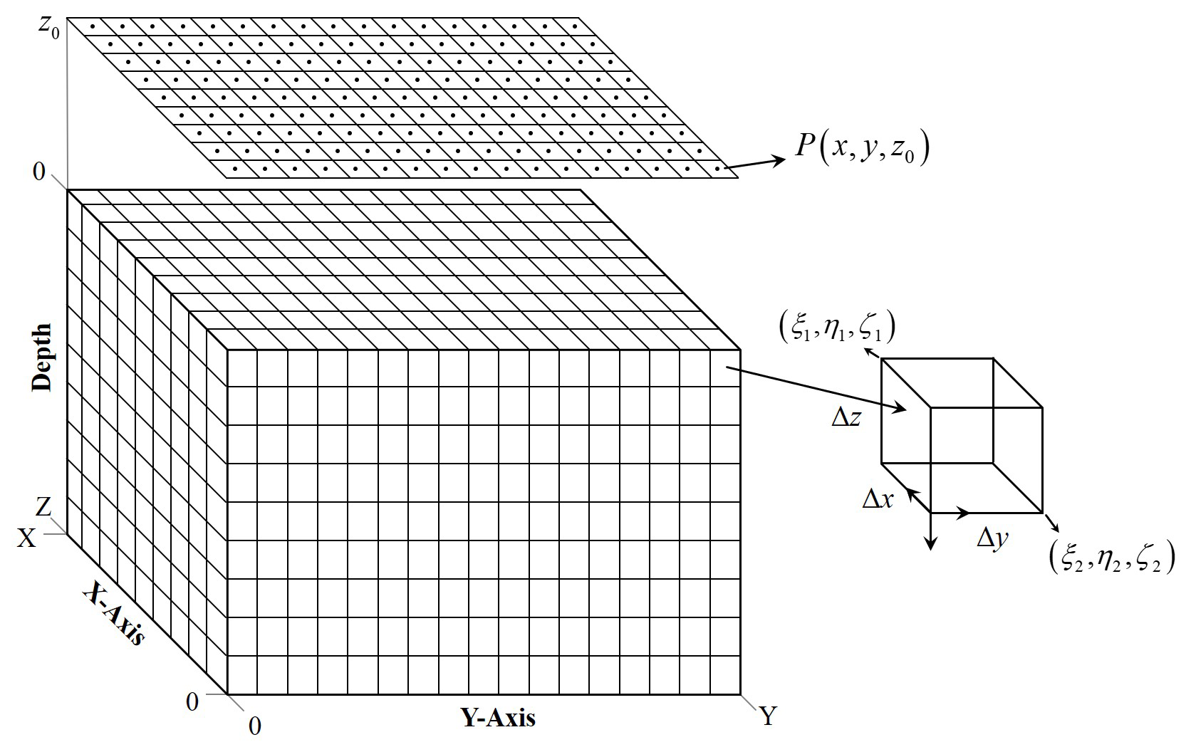
As shown in Fig. 1, a collection of rectangular prisms offers a straightforward way to approximate the volume of an anomalous body (Li and Chouteau, 1998). Each prism is assumed to have constant physical properties, such as density contrast or magnetization. For a rectangular prism whose dimensions are constrained as [ξ₁,ξ₂], [η₁,η₂], [ζ₁,ζ₂] in the x, y, and z directions (Fig. 1), according to Li and Chouteau (1998) and Nagy et al. (2000), the vertical component of the gravity attraction  Δg and the gravity gradient components V_zz, V_xx, V_yy, V_xz, V_zx, V_yz, V_zy, V_xy and V_yx at the observation point $P(x,y,z_{\mathrm{0}})$ are given by:

$$\begin{array}{}\text{(1)}& {\displaystyle }\begin{array}{rl}& \mathrm{\Delta }g(x,y,z_{\mathrm{0}})=-G\mathrm{\Delta }\mathit{\rho }\sum _{i=\mathrm{1}}^{\mathrm{2}}\sum _{j=\mathrm{1}}^{\mathrm{2}}\sum _{k=\mathrm{1}}^{\mathrm{2}}{u}_{ijk}\left[x_i\ln \right(r_{ijk}+y_j)\\ & +y_j\ln (r_{ijk}+x_i)-z_k\arctan \left({\displaystyle \frac{x_i{y}_j}{z_k{r}_{ijk}}}\right)],\end{array}\text{(2)}& {\displaystyle }{V}_{zz}(x,y,z_{\mathrm{0}})=G\mathrm{\Delta }\mathit{\rho }\sum _{i=\mathrm{1}}^{\mathrm{2}}\sum _{j=\mathrm{1}}^{\mathrm{2}}\sum _{k=\mathrm{1}}^{\mathrm{2}}{u}_{ijk}\arctan \left({\displaystyle \frac{x_i{y}_j}{z_k{r}_{ijk}}}\right),\end{array}$$

$$\begin{array}{}\text{(3)}& {\displaystyle }{V}_{xx}(x,y,z_{\mathrm{0}})=G\mathrm{\Delta }\mathit{\rho }\sum _{i=\mathrm{1}}^{\mathrm{2}}\sum _{j=\mathrm{1}}^{\mathrm{2}}\sum _{k=\mathrm{1}}^{\mathrm{2}}{u}_{ijk}\arctan \left({\displaystyle \frac{y_j{z}_k}{x_i{r}_{ijk}}}\right),\text{(4)}& {\displaystyle }{V}_{yy}(x,y,z_{\mathrm{0}})=G\mathrm{\Delta }\mathit{\rho }\sum _{i=\mathrm{1}}^{\mathrm{2}}\sum _{j=\mathrm{1}}^{\mathrm{2}}\sum _{k=\mathrm{1}}^{\mathrm{2}}{u}_{ijk}\arctan \left({\displaystyle \frac{x_i{z}_k}{y_j{r}_{ijk}}}\right),\text{(5)}& {\displaystyle }\begin{array}{rl}& V_{xz}(x,y,z_{\mathrm{0}})=V_{zx}(x,y,z_{\mathrm{0}})\\ & =-G\mathrm{\Delta }\mathit{\rho }\sum _{i=\mathrm{1}}^{\mathrm{2}}\sum _{j=\mathrm{1}}^{\mathrm{2}}\sum _{k=\mathrm{1}}^{\mathrm{2}}{u}_{ijk}\ln (r_{ijk}+y_j),\end{array}\text{(6)}& {\displaystyle }\begin{array}{rl}& V_{yz}(x,y,z_{\mathrm{0}})=V_{zy}(x,y,z_{\mathrm{0}})\\ & =-G\mathrm{\Delta }\mathit{\rho }\sum _{i=\mathrm{1}}^{\mathrm{2}}\sum _{j=\mathrm{1}}^{\mathrm{2}}\sum _{k=\mathrm{1}}^{\mathrm{2}}{u}_{ijk}\ln (r_{ijk}+x_i),\end{array}\text{(7)}& {\displaystyle }\begin{array}{rl}& V_{xy}(x,y,z_{\mathrm{0}})=V_{yx}(x,y,z_{\mathrm{0}})\\ & =-G\mathrm{\Delta }\mathit{\rho }\sum _{i=\mathrm{1}}^{\mathrm{2}}\sum _{j=\mathrm{1}}^{\mathrm{2}}\sum _{k=\mathrm{1}}^{\mathrm{2}}{u}_{ijk}\ln (r_{ijk}+z_k),\end{array}\end{array}$$

where G is the universal gravitational constant ($\mathrm{6.672}\times {\mathrm{10}}^{-\mathrm{11}}{\mathrm{m}}^{\mathrm{3}}{\mathrm{kg}}^{-\mathrm{1}}{\mathrm{s}}^{-\mathrm{2}}$), Δρ is the density contrast of the rectangular prism, $x_i=x-{\mathit{\xi }}_i$, $y_j=y-{\mathit{\eta }}_j$, $z_k=z_{\mathrm{0}}-{\mathit{\zeta }}_k$, $r_{ijk}=\sqrt{x_i^{\mathrm{2}}+y_j^{\mathrm{2}}+z_k^{\mathrm{2}}}$, and $u_{ijk}=(-\mathrm{1}{)}^{i+j+k}$. The z-axis is taken to be positive downward.

According to Luo and Yao (2007), the three components of the magnetic field anomaly $(B_x,B_y,B_z)$ and its gradient tensors due to the prism at the observation point $P(x,y,z_{\mathrm{0}})$ are given by:

$$\begin{array}{}\text{(8)}& {\displaystyle }& {\displaystyle }\begin{array}{rl}{\displaystyle }{B}_x(x,y,z_{\mathrm{0}})& {\displaystyle }={\displaystyle \frac{{\mathit{\mu }}_{\mathrm{0}}M}{\mathrm{4}\mathit{\pi }}}{\sum }_{i=\mathrm{1}}^{\mathrm{2}}{\sum }_{j=\mathrm{1}}^{\mathrm{2}}{\sum }_{k=\mathrm{1}}^{\mathrm{2}}{u}_{ijk}\\ {\displaystyle }& {\displaystyle }\times [-k_{\mathrm{1}}\arctan \left({\displaystyle \frac{y_j{z}_k}{x_i{r}_{ijk}}}\right)+k_{\mathrm{2}}\ln (r_{ijk}+z_k)\\ {\displaystyle }& {\displaystyle }+k_{\mathrm{3}}\ln (r_{ijk}+y_j)],\end{array}\text{(9)}& {\displaystyle }& {\displaystyle }\begin{array}{rl}{\displaystyle }{B}_y(x,y,z_{\mathrm{0}})& {\displaystyle }={\displaystyle \frac{{\mathit{\mu }}_{\mathrm{0}}M}{\mathrm{4}\mathit{\pi }}}{\sum }_{i=\mathrm{1}}^{\mathrm{2}}{\sum }_{j=\mathrm{1}}^{\mathrm{2}}{\sum }_{k=\mathrm{1}}^{\mathrm{2}}{u}_{ijk}\\ {\displaystyle }& {\displaystyle }\times \left[k_{\mathrm{1}}\ln \right(r_{ijk}+z_k)-k_{\mathrm{2}}\arctan \left({\displaystyle \frac{x_i{z}_k}{y_j{r}_{ijk}}}\right)\\ {\displaystyle }& {\displaystyle }+k_{\mathrm{3}}\ln (r_{ijk}+x_i)],\end{array}\text{(10)}& {\displaystyle }& {\displaystyle }\begin{array}{rl}{\displaystyle }{B}_z(x,y,z_{\mathrm{0}})& {\displaystyle }={\displaystyle \frac{{\mathit{\mu }}_{\mathrm{0}}M}{\mathrm{4}\mathit{\pi }}}{\sum }_{i=\mathrm{1}}^{\mathrm{2}}{\sum }_{j=\mathrm{1}}^{\mathrm{2}}{\sum }_{k=\mathrm{1}}^{\mathrm{2}}{u}_{ijk}\\ {\displaystyle }& {\displaystyle }\times \left[k_{\mathrm{1}}\ln \right(r_{ijk}+y_j)+k_{\mathrm{2}}\ln (r_{ijk}+x_i)-k_{\mathrm{3}}\\ {\displaystyle }& {\displaystyle }\times \arctan \left({\displaystyle \frac{x_i{y}_j}{z_k{r}_{ijk}}}\right)],\end{array}\text{(11)}& {\displaystyle }& {\displaystyle }\begin{array}{rl}{\displaystyle }{B}_{xx}(x,y,z_{\mathrm{0}})& {\displaystyle }=-{\displaystyle \frac{{\mathit{\mu }}_{\mathrm{0}}M}{\mathrm{4}\mathit{\pi }}}{\sum }_{i=\mathrm{1}}^{\mathrm{2}}{\sum }_{j=\mathrm{1}}^{\mathrm{2}}{\sum }_{k=\mathrm{1}}^{\mathrm{2}}{u}_{ijk}\\ {\displaystyle }& {\displaystyle }\times [k_{\mathrm{1}}{\displaystyle \frac{y_j{z}_k\left(r_{ijk}^{\mathrm{2}}+x_i^{\mathrm{2}}\right)}{\left(x_i^{\mathrm{2}}+z_k^{\mathrm{2}}\right)\left(x_i^{\mathrm{2}}+y_j^{\mathrm{2}}\right)r_{ijk}}}\\ {\displaystyle }& {\displaystyle }+k_{\mathrm{2}}{\displaystyle \frac{x_i}{r_{ijk}(r_{ijk}+z_k)}}+k_{\mathrm{3}}{\displaystyle \frac{x_i}{r_{ijk}(r_{ijk}+y_j)}}],\end{array}\text{(12)}& {\displaystyle }& {\displaystyle }\begin{array}{rl}{\displaystyle }{B}_{yy}(x,y,z_{\mathrm{0}})& {\displaystyle }=-{\displaystyle \frac{{\mathit{\mu }}_{\mathrm{0}}M}{\mathrm{4}\mathit{\pi }}}{\sum }_{i=\mathrm{1}}^{\mathrm{2}}{\sum }_{j=\mathrm{1}}^{\mathrm{2}}{\sum }_{k=\mathrm{1}}^{\mathrm{2}}{u}_{ijk}\\ {\displaystyle }& {\displaystyle }\times [k_{\mathrm{1}}{\displaystyle \frac{y_j}{r_{ijk}(r_{ijk}+z_k)}}\\ {\displaystyle }& {\displaystyle }+k_{\mathrm{2}}{\displaystyle \frac{x_i{z}_k\left(r_{ijk}^{\mathrm{2}}+y_j^{\mathrm{2}}\right)}{\left(y_j^{\mathrm{2}}+z_k^{\mathrm{2}}\right)\left(x_i^{\mathrm{2}}+y_j^{\mathrm{2}}\right)r_{ijk}}}\\ {\displaystyle }& {\displaystyle }+k_{\mathrm{3}}{\displaystyle \frac{y_j}{r_{ijk}\left(r_{ijk}+x_i\right)}}],\end{array}\text{(13)}& {\displaystyle }& {\displaystyle }\begin{array}{rl}{\displaystyle }{B}_{zz}(x,y,z_{\mathrm{0}})& {\displaystyle }=-{\displaystyle \frac{{\mathit{\mu }}_{\mathrm{0}}M}{\mathrm{4}\mathit{\pi }}}{\sum }_{i=\mathrm{1}}^{\mathrm{2}}{\sum }_{j=\mathrm{1}}^{\mathrm{2}}{\sum }_{k=\mathrm{1}}^{\mathrm{2}}{u}_{ijk}\\ {\displaystyle }& {\displaystyle }\times [k_{\mathrm{1}}{\displaystyle \frac{z_k}{r_{ijk}(r_{ijk}+y_j)}}+k_{\mathrm{2}}{\displaystyle \frac{z_k}{r_{ijk}(r_{ijk}+x_i)}}\\ {\displaystyle }& {\displaystyle }+k_{\mathrm{3}}{\displaystyle \frac{x_i{y}_j\left(r_{ijk}^{\mathrm{2}}+z_k^{\mathrm{2}}\right)}{\left(x_i^{\mathrm{2}}+z_k^{\mathrm{2}}\right)\left(y_j^{\mathrm{2}}+z_k^{\mathrm{2}}\right)r_{ijk}}}],\end{array}\end{array}$$

$$\begin{array}{}\text{(14)}& {\displaystyle }& {\displaystyle }\begin{array}{rl}{\displaystyle }{B}_{xy}(x,y,z_{\mathrm{0}})& {\displaystyle }=B_{yx}(x,y,z_{\mathrm{0}})\\ {\displaystyle }& {\displaystyle }=-{\displaystyle \frac{{\mathit{\mu }}_{\mathrm{0}}M}{\mathrm{4}\mathit{\pi }}}{\sum }_{i=\mathrm{1}}^{\mathrm{2}}{\sum }_{j=\mathrm{1}}^{\mathrm{2}}{\sum }_{k=\mathrm{1}}^{\mathrm{2}}{u}_{ijk}\\ {\displaystyle }& {\displaystyle }[k_{\mathrm{1}}{\displaystyle \frac{x_i}{r_{ijk}\left(r_{ijk}+z_k\right)}}+k_{\mathrm{2}}{\displaystyle \frac{y_j}{r_{ijk}(r_{ijk}+z_k)}}\\ {\displaystyle }& {\displaystyle }+k_{\mathrm{3}}{\displaystyle \frac{\mathrm{1}}{r_{ijk}}}],\end{array}\text{(15)}& {\displaystyle }& {\displaystyle }\begin{array}{rl}{\displaystyle }{B}_{yz}(x,y,z_{\mathrm{0}})& {\displaystyle }=B_{zy}(x,y,z_{\mathrm{0}})\\ {\displaystyle }& {\displaystyle }=-{\displaystyle \frac{{\mathit{\mu }}_{\mathrm{0}}M}{\mathrm{4}\mathit{\pi }}}{\sum }_{i=\mathrm{1}}^{\mathrm{2}}{\sum }_{j=\mathrm{1}}^{\mathrm{2}}{\sum }_{k=\mathrm{1}}^{\mathrm{2}}{u}_{ijk}[k_{\mathrm{1}}{\displaystyle \frac{\mathrm{1}}{r_{ijk}}}\\ {\displaystyle }& {\displaystyle }+k_{\mathrm{2}}{\displaystyle \frac{y_j}{r_{ijk}(r_{ijk}+x_i)}}+k_{\mathrm{3}}{\displaystyle \frac{z_k}{r_{ijk}(r_{ijk}+x_i)}}],\end{array}\text{(16)}& {\displaystyle }& {\displaystyle }\begin{array}{rl}{\displaystyle }{B}_{xz}(x,y,z_{\mathrm{0}})& {\displaystyle }=B_{zx}(x,y,z_{\mathrm{0}})=\\ {\displaystyle }& {\displaystyle }-{\displaystyle \frac{{\mathit{\mu }}_{\mathrm{0}}M}{\mathrm{4}\mathit{\pi }}}{\sum }_{i=\mathrm{1}}^{\mathrm{2}}{\sum }_{j=\mathrm{1}}^{\mathrm{2}}{\sum }_{k=\mathrm{1}}^{\mathrm{2}}{u}_{ijk}\\ {\displaystyle }& {\displaystyle }[k_{\mathrm{1}}{\displaystyle \frac{x_i}{r_{ijk}(r_{ijk}+y_j)}}+k_{\mathrm{2}}{\displaystyle \frac{\mathrm{1}}{r_{ijk}}}+k_{\mathrm{3}}{\displaystyle \frac{z_k}{r_{ijk}(r_{ijk}+y_j)}}],\end{array}\end{array}$$

where M is the induced magnetization intensity of the rectangular prism with the inclination (I^′) and declination (D^′), $k_{\mathrm{1}}=\cos I^{\prime }\cos D^{\prime }$, $k_{\mathrm{2}}=\cos I^{\prime }\sin D^{\prime }$, $k_{\mathrm{3}}=\sin I^{\prime }$, ${\mathit{\mu }}_{\mathrm{0}}=\mathrm{4}\mathit{\pi }\times {\mathrm{10}}^{-\mathrm{7}}\mathrm{H}{\mathrm{m}}^{-\mathrm{1}}$ is the magnetic permeability of the vacuum.

Suppose the magnetic anomaly caused by a magnetic body is small compared with the Earth's main magnetic field. Then the scalar magnitude of the magnetic field anomalies can be approximately calculated by projecting the components of the anomalous field in the direction of the Earth's main magnetic field (Hinze et al., 2013; Plouff, 1976). As a result, the total magnetic intensity anomaly ΔT and its gradients $(\mathrm{\Delta }{T}_x,\mathrm{\Delta }{T}_y,\mathrm{\Delta }{T}_z)$ from the source can be approximated by:

$$\begin{array}{}\text{(17)}& {\displaystyle }& {\displaystyle }\mathrm{\Delta }T=B_x\cos I\cos D+B_y\cos I\sin D+B_z\sin I,\text{(18)}& {\displaystyle }& {\displaystyle }\mathrm{\Delta }{T}_x=B_{xx}\cos I\cos D+B_{yx}\cos I\sin D+B_{zx}\sin I,\text{(19)}& {\displaystyle }& {\displaystyle }\mathrm{\Delta }{T}_y=B_{xy}\cos I\cos D+B_{yy}\cos I\sin D+B_{zy}\sin I,\text{(20)}& {\displaystyle }& {\displaystyle }\mathrm{\Delta }{T}_z=B_{xz}\cos I\cos D+B_{yz}\cos I\sin D+B_{zz}\sin I,\end{array}$$

where I and D are the inclination and declination of the Earth's geomagnetic field at the observation point.

2.2 Fast forward modelling method

In G&M3D 1.0, we define a source region with the range [0,X], [0,Y], and [0,Z] in the x, y, and z axes, respectively. The source space is divided into $N\times M\times L$ prisms, each with dimensions of $\mathrm{\Delta }x\times \mathrm{\Delta }y\times \mathrm{\Delta }z$. These prisms are labeled as $(a,b,c)$, with their dimensions limited to $[{\mathit{\xi }}_{\mathrm{1},a}=(a-\mathrm{1})\mathrm{\Delta }x,{\mathit{\xi }}_{\mathrm{2},a}=a\mathrm{\Delta }x]$, $[{\mathit{\eta }}_{\mathrm{1},b}=(b-\mathrm{1})\mathrm{\Delta }y,{\mathit{\eta }}_{\mathrm{2},b}=b\mathrm{\Delta }y]$, $[{\mathit{\zeta }}_{\mathrm{1},c}=(c-\mathrm{1})\mathrm{\Delta }z,{\mathit{\zeta }}_{\mathrm{2},c}=c\mathrm{\Delta }z]$, where $a=\mathrm{1},\mathrm{2},\mathrm{\dots },N$; $b=\mathrm{1},\mathrm{2},\mathrm{\dots },M$; $c=\mathrm{1},\mathrm{2},\mathrm{\dots },L$.

The observation points $P(x_n,y_m,z_{\mathrm{0}})$, where $x_n=(n-\mathrm{0.5})\mathrm{\Delta }x$, $n=\mathrm{1},\mathrm{\dots },N$, $y_m=(m-\mathrm{0.5})\mathrm{\Delta }y$, $m=\mathrm{1},\mathrm{\dots },M$, are distributed at the horizontal surface z₀ at regular intervals, aligned with the prism centers, as shown in Fig. 1. The gravity/magnetic fields at the observation point $P(x_n,y_m,z_{\mathrm{0}})$ can be calculated by summing the contributions from all prisms within the source region:

$$\begin{array}{}\text{(21)}& \begin{array}{rl}{\displaystyle }& {\displaystyle }g(x_n,y_m,z_{\mathrm{0}})=\\ {\displaystyle }& {\displaystyle }{\sum }_{c=\mathrm{1}}^L\left[{\sum }_{a=\mathrm{1}}^N{\sum }_{b=\mathrm{1}}^{M}f(a,b,c)\times t(x_n,y_m,z_{\mathrm{0}},a,b,c)\right],\end{array}\end{array}$$

where $f(a,b,c)$ is the density contrast or magnetization value corresponding to the prism $(a,b,c)$, and $t(x_n,y_m,z_{\mathrm{0}},a,b,c)$ is the field response at $P(x_n,y_m,z_{\mathrm{0}})$ generated by prism $(a,b,c)$ with unit density contrast or magnetization. Therefore, t represents the kernel (or sensitivity) coefficient, which can be evaluated using any of Eqs. (1)–(16), rather than a simple distance-dependent decay term.

Thanks to Eq. (21), the gravity/magnetic field at all observation points can be presented in matrix-vector form as follows,

$$\begin{array}{}\text{(22)}& \mathit{g}=\mathbf{K}\cdot \mathit{f},\end{array}$$

where g is the field vector, f is the density contrast or magnetization parameter vector, K represents the kernel matrix (or sensitivity matrix) with dimension $(N\times M)\times (N\times M\times L)$, which is classified as a Block–Toeplitz Toeplitz–Block (BTTB) matrix.

The forward calculations described in Eq. (22) can be time-consuming, particularly when the source space is large and finely discretized. In this study, we apply a 2D discrete convolution algorithm using block circulant extension (BCE) (Chen and Liu, 2019) to optimize the forward calculations. In G&M3D 1.0, we conduct forward calculations of potential fields layer by layer along the z direction using the BCE algorithm. The procedure for the BCE algorithm (Chen and Liu, 2019) is as follows.

First, the density contrast or magnetization values of all the prisms are stored in a 3D matrix E of size $N\times M\times L$. For any given layer (e.g., the cth layer, $c=\mathrm{1},\mathrm{\dots },L$), the parameter matrix is defined as $\mathbf{f}=\mathit{E}(\mathrm{1}:N,\mathrm{1}:M,c)$. A null parameter matrix f (where all elements equal zero) indicates that the prisms in the cth layer make no contribution to the observed field. For non-zero cases, the matrix f is extended with zeros to form an extended parameter matrix F,

$$\begin{array}{}\text{(23)}& \mathbf{F}=\left[\begin{array}{cc}\mathbf{f}& {\mathbf{0}}_{N\times M}\\ {\mathbf{0}}_{N\times M}& {\mathbf{0}}_{N\times M}\end{array}\right]\end{array}$$

Next, to implement the BCE-based discrete convolution, the observation range is extended along the negative directions of the x-axis and y-axis from [0,X], [0,Y] to $[-X+\mathrm{\Delta }x,X]$, $[-Y+\mathrm{\Delta }y,Y]$, as shown in Fig. 2. This extension is necessary because Eq. (21) represents a linear convolution, whereas the FFT inherently evaluates a circular convolution. By embedding the original problem into an extended domain, the linear convolution can be reformulated in a circulant form and computed efficiently without introducing wrap-around boundary errors at the boundaries. We then compute the field effects generated by the prism $(a=\mathrm{1},b=\mathrm{1},c)$ (dimensions limited as $[{\mathit{\xi }}_{\mathrm{1}}=\mathrm{0},{\mathit{\xi }}_{\mathrm{2}}=\mathrm{\Delta }x]$, $[{\mathit{\eta }}_{\mathrm{1}}=\mathrm{0},{\mathit{\eta }}_{\mathrm{2}}=\mathrm{\Delta }y]$, $[{\mathit{\zeta }}_{\mathrm{1}}=(c-\mathrm{1})\mathrm{\Delta }z,{\mathit{\zeta }}_{\mathrm{2}}=c\mathrm{\Delta }z])$ at all observation points in the extended area. Note that the extended area serves only as an auxiliary computational domain; only the results within the original observation region are retained. This results in an extended response matrix T with a size of $(\mathrm{2}N-\mathrm{1})\times (\mathrm{2}M-\mathrm{1})$ for the cth layer,

$$\begin{array}{}\text{(24)}& \mathbf{T}=\left[\begin{array}{ccc}{t}_{\mathrm{1},\mathrm{1}}& \mathrm{\cdots }& t_{\mathrm{1},\mathrm{2}M-\mathrm{1}}\\ \mathrm{⋮}& t_{n^{\prime },m^{\prime }}& \mathrm{⋮}\\ t_{\mathrm{2}N-\mathrm{1},\mathrm{1}}& \mathrm{\cdots }& t_{\mathrm{2}N-\mathrm{1},\mathrm{2}M-\mathrm{1}}\end{array}\right],\end{array}$$

where $t_{n^{\prime },m^{\prime }}(n^{\prime }=\mathrm{1},\mathrm{2},\mathrm{\dots },\mathrm{2}N-\mathrm{1};m^{\prime }=\mathrm{1},\mathrm{2},\mathrm{\dots },\mathrm{2}M-\mathrm{1})$ is the field response at the observation $P(x_{n^{\prime }},y_{m^{\prime }},z_{\mathrm{0}})$ where $x_{n^{\prime }}=(n^{\prime }-N-\mathrm{0.5})\mathrm{\Delta }x$, $y_{m^{\prime }}=(m^{\prime }-M-\mathrm{0.5})\mathrm{\Delta }y$, which is calculated using Eqs. (1)–(16) with unit density contrast or induced magnetization intensity (namely, Δρ=1, M=1).

We extend T by zeros along the top and the left margins, as shown in Fig. 2. This creates a matrix T₀ with a size of 2N×2M,

$$\begin{array}{}\text{(25)}& {\mathbf{T}}_{\mathrm{0}}=\left[\begin{array}{cc}\mathrm{0}& {\mathbf{0}}_{\mathrm{1}\times (\mathrm{2}M-\mathrm{1})}\\ {\mathbf{0}}_{(\mathrm{2}N-\mathrm{1})\times \mathrm{1}}& \mathbf{T}\end{array}\right].\end{array}$$

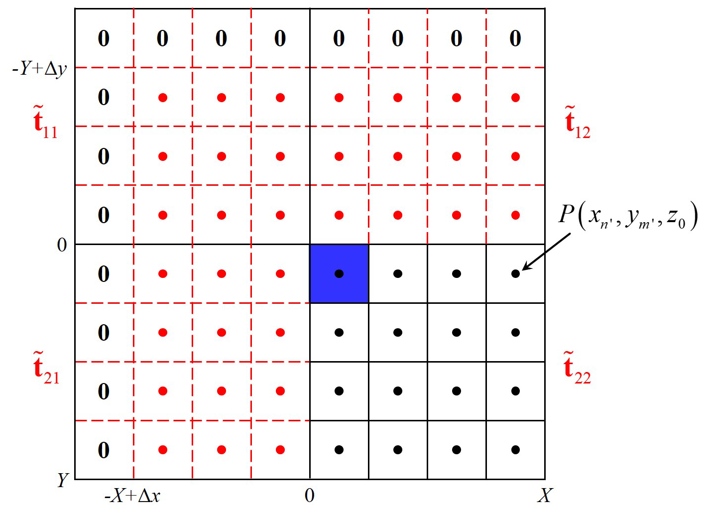
Figure 2 The sketch map shows the extended observation points and source region for the BCE method. The extended observation points are shown in red, and the observation points in the original observation domain are shown in black. The prism (1,1) is marked in blue. A single-layer model consisting of 4×4 prisms is taken as an example.

The matrix T₀ in Eq. (25) can then be rewritten into four N×M submatrices as,

$$\begin{array}{}\text{(26)}& {\mathbf{T}}_{\mathrm{0}}=\left[\begin{array}{cc}{\stackrel{\mathrm{̃}}{\mathbf{t}}}_{\mathrm{11}}& {\stackrel{\mathrm{̃}}{\mathbf{t}}}_{\mathrm{12}}\\ {\stackrel{\mathrm{̃}}{\mathbf{t}}}_{\mathrm{21}}& {\stackrel{\mathrm{̃}}{\mathbf{t}}}_{\mathrm{22}}\end{array}\right].\end{array}$$

By reordering the submatrices in Eq. (26), we get

$$\begin{array}{}\text{(27)}& \mathbf{C}=\left[\begin{array}{cc}{\stackrel{\mathrm{̃}}{\mathbf{t}}}_{\mathrm{22}}& {\stackrel{\mathrm{̃}}{\mathbf{t}}}_{\mathrm{21}}\\ {\stackrel{\mathrm{̃}}{\mathbf{t}}}_{\mathrm{12}}& {\stackrel{\mathrm{̃}}{\mathbf{t}}}_{\mathrm{11}}\end{array}\right].\end{array}$$

The matrix C in Eq. (27) is identified as a Block–Cyclic–Cyclic–Block (BCCB) matrix. The 2D discrete convolution of this matrix with the extended parameter matrix F can be efficiently computed using the fast Fourier transform (Chen and Liu, 2019; Vogel, 2002) as follows,

$$\begin{array}{}\text{(28)}& {\displaystyle }& {\displaystyle }\stackrel{\mathrm{̃}}{\mathbf{C}}=\text{fft}\mathrm{2}\left(\mathbf{C}\right),\text{(29)}& {\displaystyle }& {\displaystyle }\stackrel{\mathrm{̃}}{\mathbf{F}}=\text{fft}\mathrm{2}\left(\mathbf{F}\right),\text{(30)}& {\displaystyle }& {\displaystyle }\stackrel{\mathrm{̃}}{\mathbf{G}}=\stackrel{\mathrm{̃}}{\mathbf{C}}.\ast \stackrel{\mathrm{̃}}{\mathbf{F}},\text{(31)}& {\displaystyle }& {\displaystyle }\mathbf{G}=\text{ifft}\mathrm{2}\left(\stackrel{\mathrm{̃}}{\mathbf{G}}\right),\text{(32)}& {\displaystyle }& {\displaystyle }{\mathbf{G}}_c=\mathbf{G}(\mathrm{1}:N,\mathrm{1}:M),\end{array}$$

where fft2 is the 2D fast Fourier transform, and ifft2 denotes the 2D inverse fast Fourier transform. The symbol $.\ast$ represents the dot multiplication operator. G_c is the resulting field at the observations generated by the anomalous prisms in the cth layer.

Repeat these steps for each layer, and the total field g at all observations is obtained by,

$$\begin{array}{}\text{(33)}& \mathit{g}=\sum _{c=\mathrm{1}}^L{\mathbf{G}}_c.\end{array}$$

From a programming perspective, we implement two strategies to enhance computational efficiency in G&M3D 1.0.

2.2.1 Strategy 1

We take advantage of the fast matrix operation in Qt to optimize the forward calculations in G&M3D 1.0. We construct in advance two new matrices X_i and Y_j with sizes of $(\mathrm{2}N-\mathrm{1})\times (\mathrm{2}M-\mathrm{1})$,

$$\begin{array}{}\text{(34)}& {\displaystyle }& {\displaystyle }{\displaystyle }{\mathbf{X}}_i=\left[\begin{array}{ccc}{x}_{\mathrm{1}}& \mathrm{\cdots }& x_{\mathrm{1}}\\ \mathrm{⋮}& x_{n^{\prime }}& \mathrm{⋮}\\ x_{\mathrm{2}N-\mathrm{1}}& \mathrm{\cdots }& x_{\mathrm{2}N-\mathrm{1}}\end{array}\right]-{\mathit{\xi }}_i\mathbf{I},\text{(35)}& {\displaystyle }& {\displaystyle }{\displaystyle }{\mathbf{Y}}_j=\left[\begin{array}{ccc}{y}_{\mathrm{1}}& \mathrm{\cdots }& y_{\mathrm{2}M-\mathrm{1}}\\ \mathrm{⋮}& y_{m^{\prime }}& \mathrm{⋮}\\ y_{\mathrm{1}}& \mathrm{\cdots }& y_{\mathrm{2}M-\mathrm{1}}\end{array}\right]-{\mathit{\eta }}_j\mathbf{I},\end{array}$$

where $i,j=\mathrm{1},\mathrm{2}$, $x_{n^{\prime }}=(n^{\prime }-N+\mathrm{0.5})\mathrm{\Delta }x$, $y_{m^{\prime }}=(m^{\prime }-M+\mathrm{0.5})\mathrm{\Delta }y$, $(n^{\prime }=\mathrm{1},\mathrm{2},\mathrm{\dots },\mathrm{2}N-\mathrm{1}$; $m^{\prime }=\mathrm{1},\mathrm{2},\mathrm{\dots },\mathrm{2}M-\mathrm{1})$, ξ₁=0, ξ₂=Δx, η₁=0, η₂=Δy. I is an all-ones matrix. Thanks to the Eqs. (32) and (33), we can substitute the matrices X_i and Y_j to x_i and y_j in any of the Eqs. (1)–(16). This allows the extended response matrix T at all observations to be computed by a single dot product in Qt, rather than relying on a large number of cyclic calculations.

2.2.2 Strategy 2

Since the kernel matrices for gravity and magnetic components under vertical magnetization are symmetric (Hogue et al., 2020), k₁ and k₂ in Eqs. (8)–(16) are zero, and only k₃ remains. In these cases, we only calculate the submatrix ${\stackrel{\mathrm{̃}}{\mathbf{t}}}_{\mathrm{22}}$ in C (Eq. 27) for these cases. The other three submatrices $({\stackrel{\mathrm{̃}}{\mathbf{t}}}_{\mathrm{11}},{\stackrel{\mathrm{̃}}{\mathbf{t}}}_{\mathrm{12}},{\stackrel{\mathrm{̃}}{\mathbf{t}}}_{\mathrm{21}})$ can be derived from ${\stackrel{\mathrm{̃}}{\mathbf{t}}}_{\mathrm{22}}$, because they share the same value or have the opposite sign as ${\stackrel{\mathrm{̃}}{\mathbf{t}}}_{\mathrm{22}}$. This strategy results in a higher efficiency for forward calculations of gravity anomalies, gravity gradient tensor, and magnetic components with vertical magnetization compared to those for the magnetic field with non-vertical magnetization. As we know, the forward calculations of magnetic fields depend on the declination and inclination of the sources. If the anomalous bodies in the source model have varying declinations or inclinations, we classify these bodies by their declinations or inclinations and perform forward calculations of each category separately.

2.3 Synthetic model tests

To verify the efficiency of the forward calculation in G&M3D 1.0, we design a synthetic model with specified density contrast and magnetization for gravity and magnetic forward calculations. The model region extends from 0–50 km along the x, y, and z axes. It consists of an anomalous body with a density contrast of 1 g cm⁻³ and an induced magnetization of 1 A m⁻¹. The center of the body is located at (25, 25, 25) km with a size of $\mathrm{25}\mathrm{km}\times \mathrm{25}\mathrm{km}\times \mathrm{20}\mathrm{km}$.

We evaluate the computation time for gravity and magnetic forward calculations at five different numerical resolutions, employing $\mathrm{50}\times \mathrm{50}\times \mathrm{50}$, $\mathrm{100}\times \mathrm{100}\times \mathrm{100}$, $\mathrm{200}\times \mathrm{200}\times \mathrm{200}$, $\mathrm{400}\times \mathrm{400}\times \mathrm{400}$, and $\mathrm{800}\times \mathrm{800}\times \mathrm{800}$ prisms in the x-, y-, and z-directions, respectively. This corresponds to grid intervals of 1000, 500, 250, 125 and 62.5 m. In these tests, the observation points are set at the horizontal positions corresponding to the prism centers. Consequently, as the numerical resolution increases, the number of observation points also grows accordingly. The absolute computation times for the forward calculation of the gravity and magnetic fields are summarized in Table 1.

Table 1 The statistics of the absolute consumption times for forward computations of the gravity and magnetic fields with five different numerical resolutions.

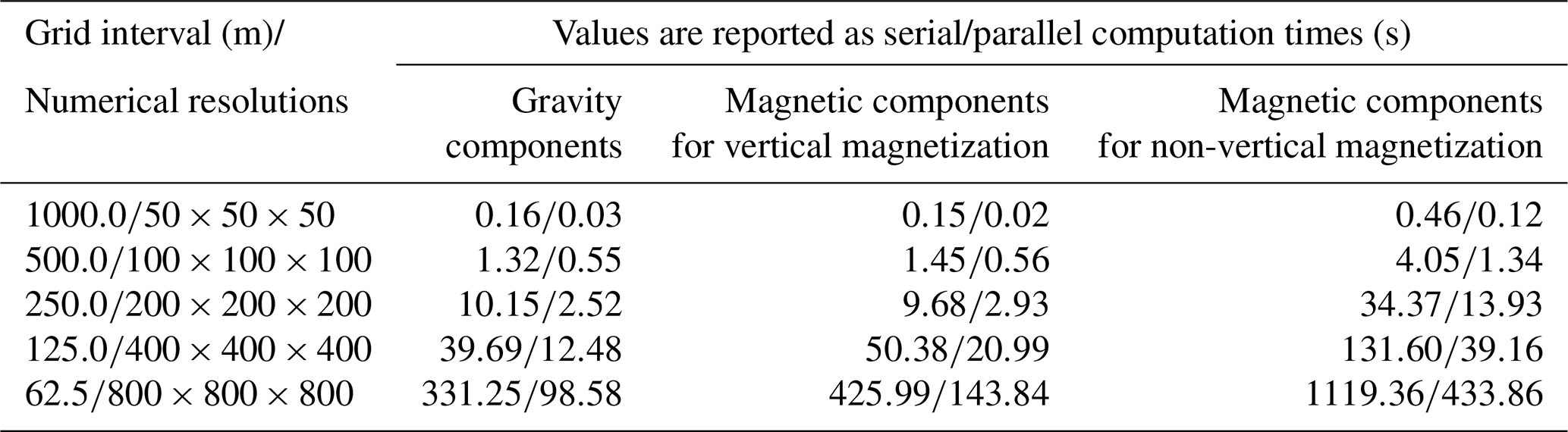
Note. All the tests are carried out on a desktop with an AMD Ryzen 7 3700X CPU (8 cores) and 32 GB of memory.

Table 1 shows that the computation time increases significantly as the numerical resolution increases. Note that the output results of the gravity calculation in Table 1 consist of 7 components, i.e., Δg, V_zz, V_xx, V_yy, V_xz, V_yz, V_xy, and the results of magnetic forward modelling include 13 components (i.e., B_x, B_y, B_z, B_xx, B_yy, B_zz, B_xy, B_xz, B_yz, ΔT, ΔT_x, ΔT_y, ΔT_z). Due to the implementation of Strategy 2, which decouples the computation of vertically and non-vertically magnetized models, the efficiency of forward modelling improves significantly. In a $\mathrm{200}\times \mathrm{200}\times \mathrm{200}$ grid case, the computation time is reduced by 71.83 % (34.37 s vs. 9.68 s). These tests demonstrate that G&M3D 1.0 is a high-speed tool for forward calculations of the gravity and magnetic fields. It is worth noting that the layers with non-zero density/magnetization occupy 40 % of the total layers in the z direction in these tests. The forward calculation is faster if the anomalous body's vertical dimension is reduced, but it requires more time if the vertical dimension increases. For example, in the $\mathrm{100}\times \mathrm{100}\times \mathrm{100}$ case, under vertical magnetization conditions, two anomalous bodies with the same number of non-zero prisms but different spatial distributions, namely $\mathrm{1}\times \mathrm{1}\times \mathrm{100}$ prisms and $\mathrm{100}\times \mathrm{1}\times \mathrm{1}$ prisms, require total computation times of about 2.65 and 0.04 s, respectively, when calculating gravity anomalies, magnetic anomalies, and the corresponding gradient components.

To further enhance the computational performance, we implement parallel computation for the layer-by-layer forward calculations along the z-direction. In the BCE framework, the field contribution of each layer is computed independently, and the final response is obtained by summing the contributions from all layers. The parallelization is realized using task-based multithreading (standard C++), where layer-wise forward responses are launched asynchronously and collected after completion. Using the same synthetic model, discretized into $\mathrm{200}\times \mathrm{200}\times \mathrm{200}$ prisms, we record the computation times under vertical magnetization conditions using 8 threads, and the computation is approximately 3.45 times faster than that of the serial implementation.

To evaluate G&M3D 1.0 against existing open-source tools, we compare its computational efficiency with SimPEG (Cockett et al., 2015). For the $\mathrm{200}\times \mathrm{200}\times \mathrm{200}$ case, the gravity forward calculation in SimPEG takes 1606.62 s, whereas G&M3D 1.0 requires only 2.52 s. Notably, at $\mathrm{800}\times \mathrm{800}\times \mathrm{800}$ resolution, SimPEG fails due to excessive memory overflow, while G&M3D 1.0 maintains robust performance.

To validate the computational accuracy of G&M3D 1.0, we design a synthetic model consisting of three buried spheres, for which analytical solutions are available. The centers of the three spheres are located at (50, 55, 50 m), (140, 75, 65 m), and (110, 155, 80 m), with radii of 20, 30 and 35 m, respectively. The density contrasts are all set to 1 g cm⁻³, and the induced magnetizations are all set to 1 A m⁻¹. The computational domain is $\mathrm{200}\mathrm{m}\times \mathrm{200}\mathrm{m}\times \mathrm{200}\mathrm{m}$, which is discretized into $\mathrm{800}\times \mathrm{800}\times \mathrm{800}$ cells. Gravity anomalies Δg and magnetic anomalies ΔT are calculated separately, and the corresponding analytical solutions serve as references. The computed and analytical results are compared in Fig. 3. As shown in Fig. 3, the differences between our results and the analytical solutions are negligible. The maximum absolute errors of the gravity and magnetic anomalies are $\mathrm{7.5}\times {\mathrm{10}}^{-\mathrm{6}}\mathrm{mGal}$ and $\mathrm{5.4}\times {\mathrm{10}}^{-\mathrm{3}}\mathrm{nT}$, respectively.

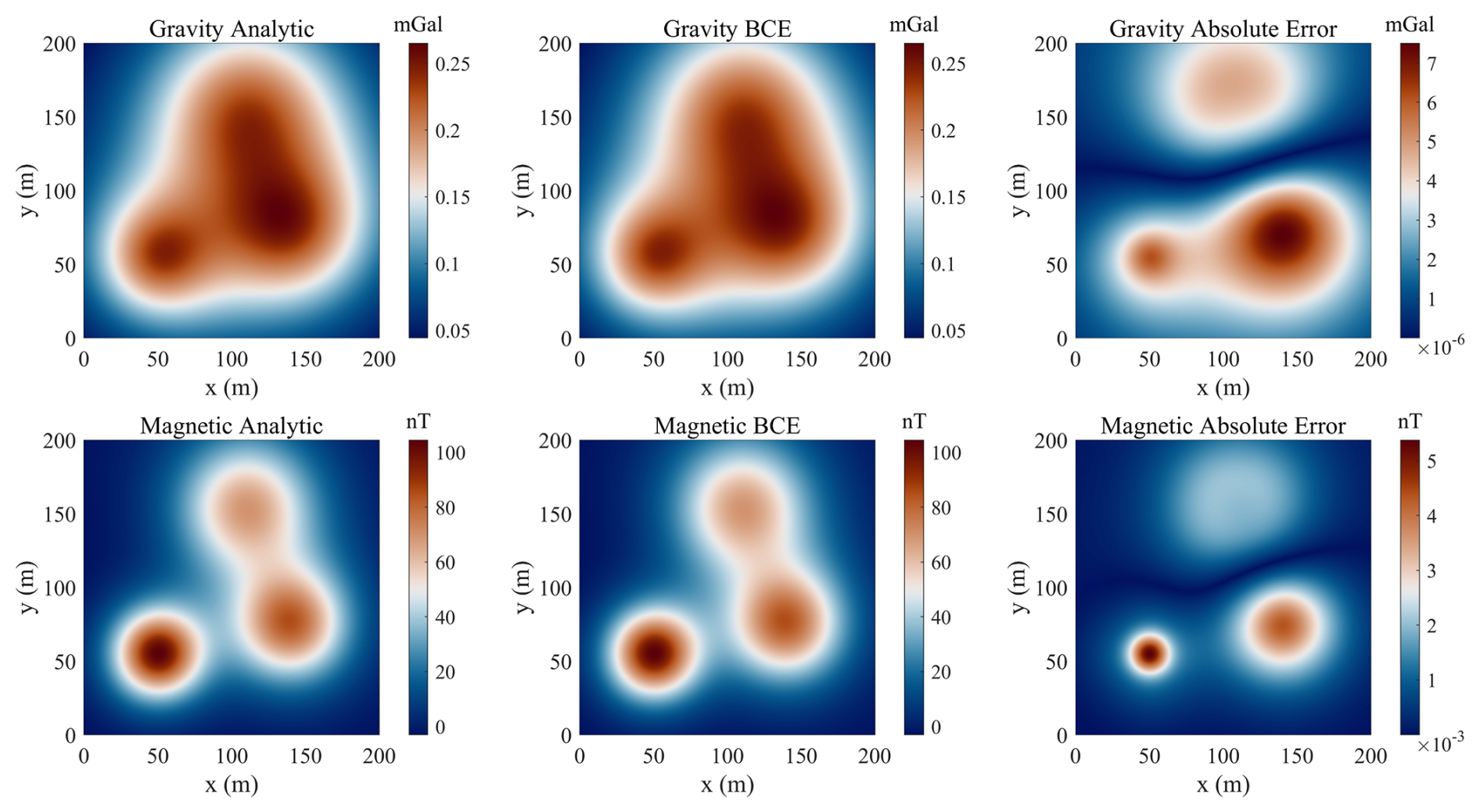
Figure 3 Comparison between analytical solutions and BCE results for gravity and magnetic anomalies produced by a synthetic model of three buried spheres.

3 The framework and functions of G&M3D

In this section, we introduce the functions and operational procedures of G&M3D 1.0. A detailed software instruction manual, including installation steps, model construction, forward modelling settings and result visualization, is provided in the Supplement. The software consists of two main modules: (1) a 3D-Modelling module for constructing source bodies and assigning physical properties, and (2) a Forward-Modelling module for calculating and visualizing the resulting gravity and magnetic fields. The workflow of G&M3D 1.0 is shown in Fig. 4. Architecturally, G&M3D 1.0 separates interactive model construction from numerical forward computation, with model data serving as an intermediate layer between the GUI and the forward-calculation kernels, thereby enhancing maintainability and extensibility. In addition, the software supports topography modelling. Users can import and visualize a topographic surface, where anomalous bodies are constrained to remain below it, and observation points can be assigned topography-dependent elevations for forward calculations over non-planar observation surfaces.

Figure 4 Workflow in G&M3D 1.0 and G&M3D 1.0 initial interface.

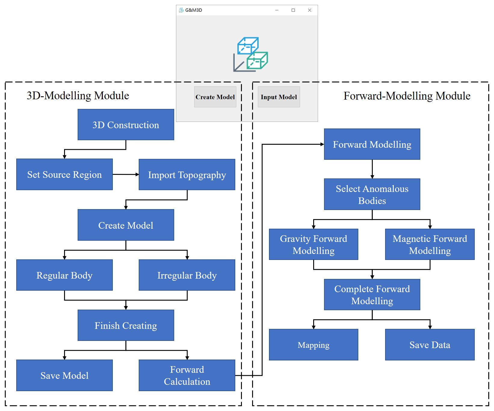
G&M3D 1.0 is based on a right-handed Cartesian coordinate system. When users open G&M3D 1.0 and enter the start interface (Fig. 4), they can access the 3D-Modelling module to create a new source model by clicking the button Create Model, or they can input an existing model data file to conduct gravity or magnetic forward calculations through the Forward-Modelling module by clicking the button Input Model.

The main interface of the Modelling module is shown in Fig. 5a. By default, G&M3D 1.0 generates an initial source region (Fig. 5b). To customize this for their needs, users should first set the source region by clicking the “Settings” button in the operation area of the main interface. In the pop-up window for the Setting Field (Fig. 5b), users can configure the basic parameters that define the source region, including the source range, mesh interval, and length unit. The supported length units are meters (m), hectometers (hm), and kilometers (km), which allow for multi-scale forward modelling simulations. If a topographic file is available, users should import it before model construction by using the “Import Topo” function in G&M3D 1.0.

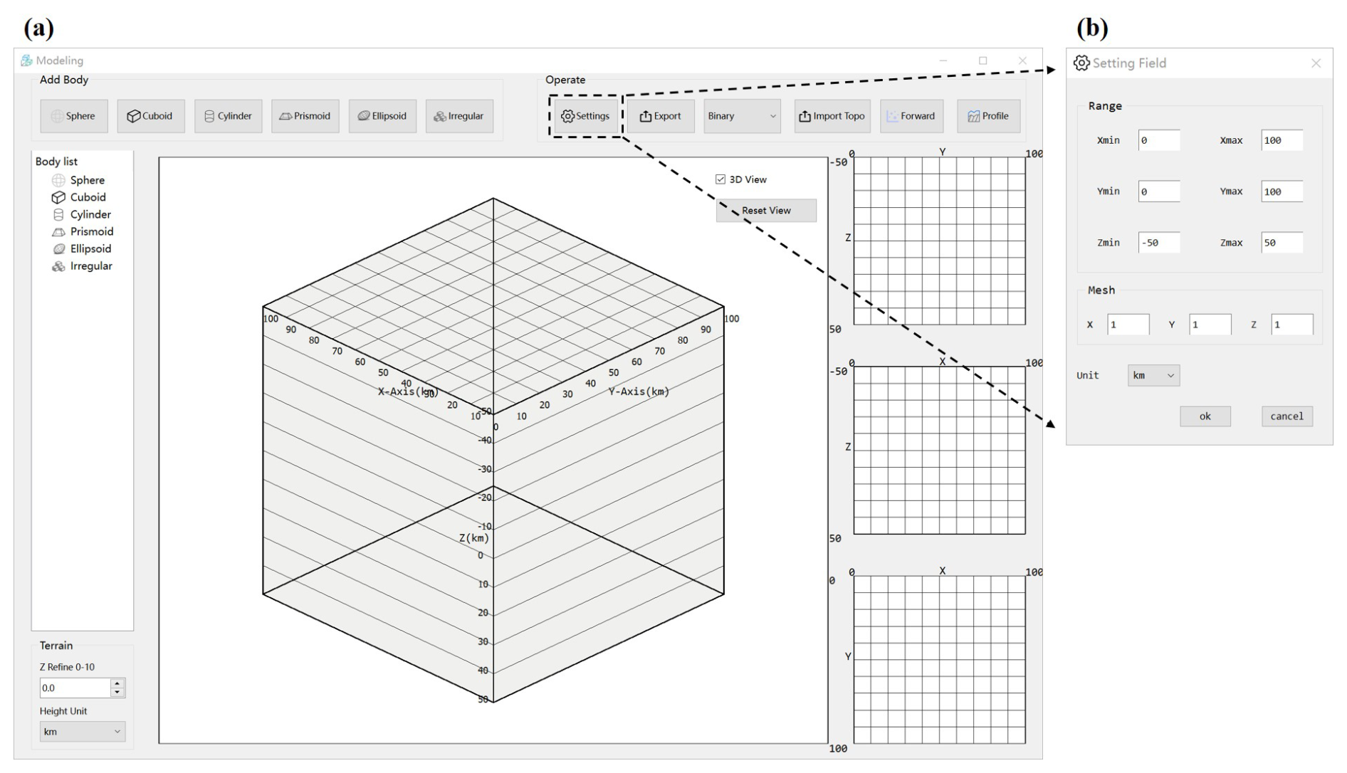
Figure 5 (a) Interface of the Modelling Module. The top functional area contains tools for creating different shapes on the left and various action buttons on the right. The middle workspace is used to display the created models (the 2D floor plan is shown in three areas on the right), and the body list is shown on the left. (b) Setting Field window showing the default initial source model settings.

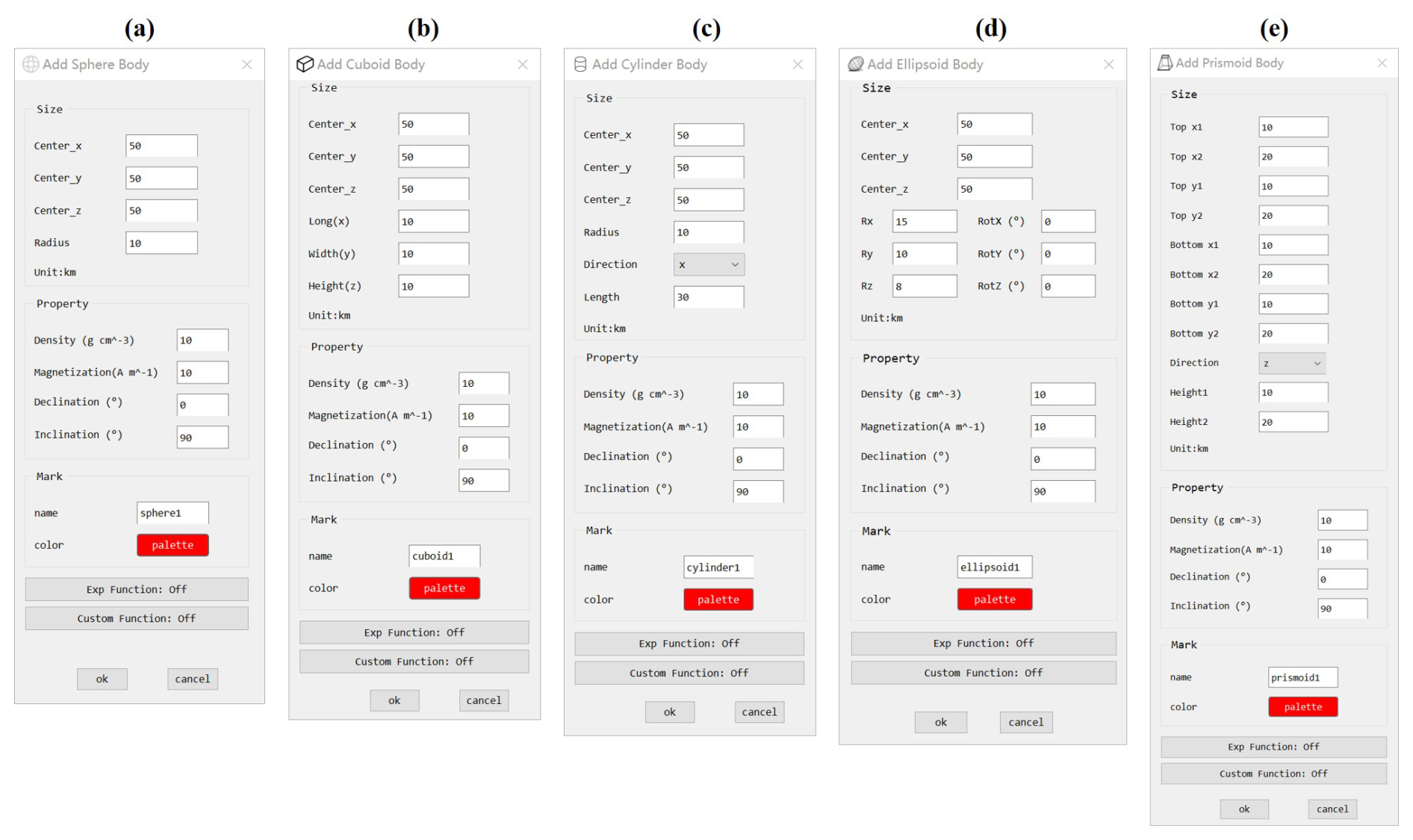
Figure 6 Parameter input interfaces for the five regular tools, including (a) Sphere, (b) Cuboid, (c) Cylinder, (d) Ellipsoid, and (e) Prismoid.

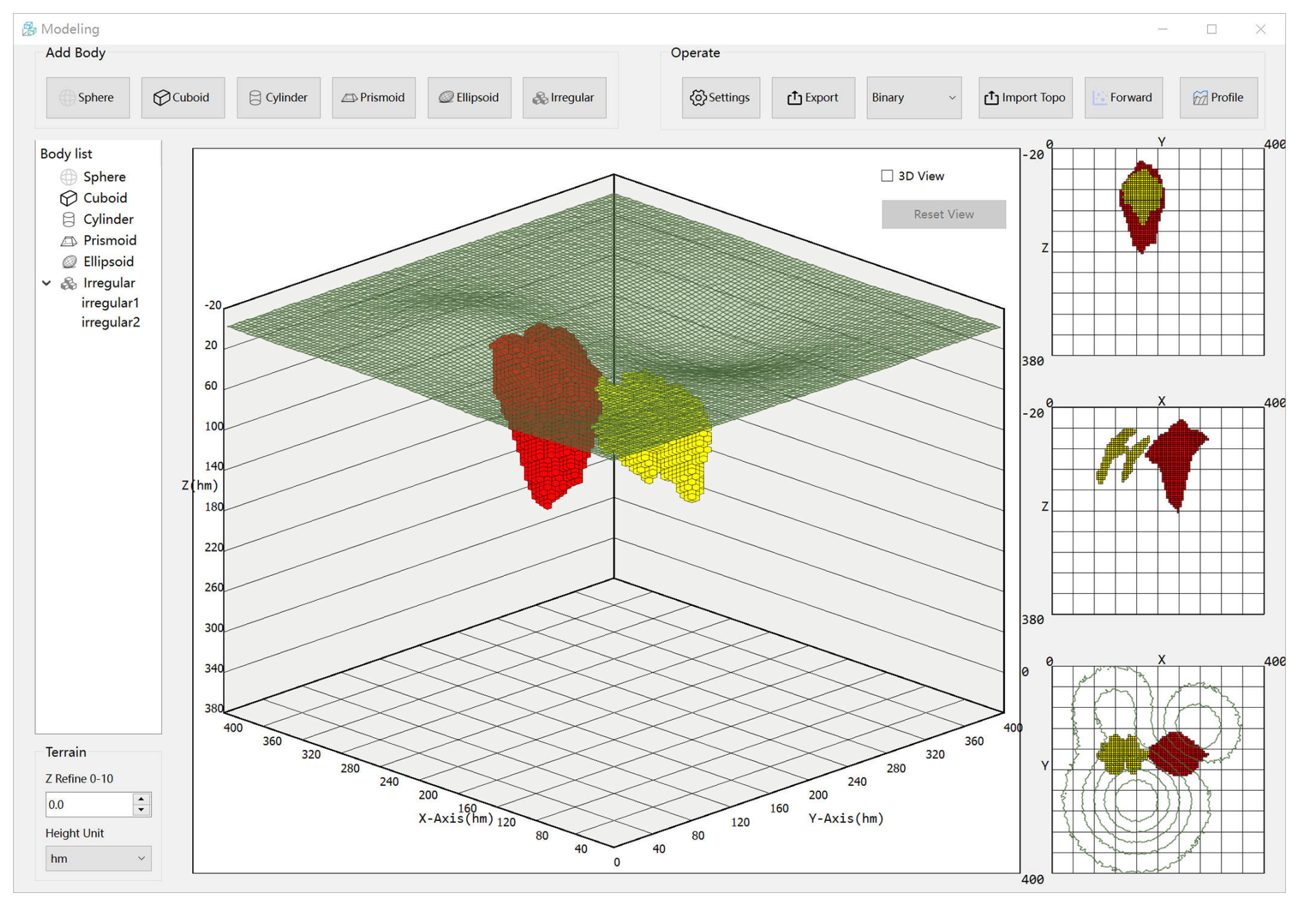
After that, users can select one of the tools on the “Add Body” panel to create anomalous bodies. G&M3D 1.0 supports sequential creation of multiple anomaly bodies, with all generated bodies automatically listed in the “Body List” section. To ensure modelling flexibility and operational efficiency, right-click functionality is provided for existing anomalies, allowing users to modify and delete them. The modification process uses the same intuitive interface as the creation process, making it just as easy to change bodies as it is to create them. G&M3D 1.0 also allows overlapping anomalous bodies. In overlapping regions, the physical properties of the later-created body overwrite those previously assigned to the corresponding prisms.

The following section explains the construction methods for regular and irregular bodies, which differ in their modelling approaches. However, both types share the same parameter configurations for gravity and magnetic properties. As shown in the “Property” panel of Fig. 6, only four parameters need to be specified: density contrast, induced magnetization intensity, magnetic declination, and magnetic inclination. Spatially heterogeneous physical-property distributions within a single body can be represented in G&M3D 1.0 through continuously varying functions. In particular, the software supports user-defined functional forms, which allow flexible construction of bodies with spatially variable density contrast or magnetization.

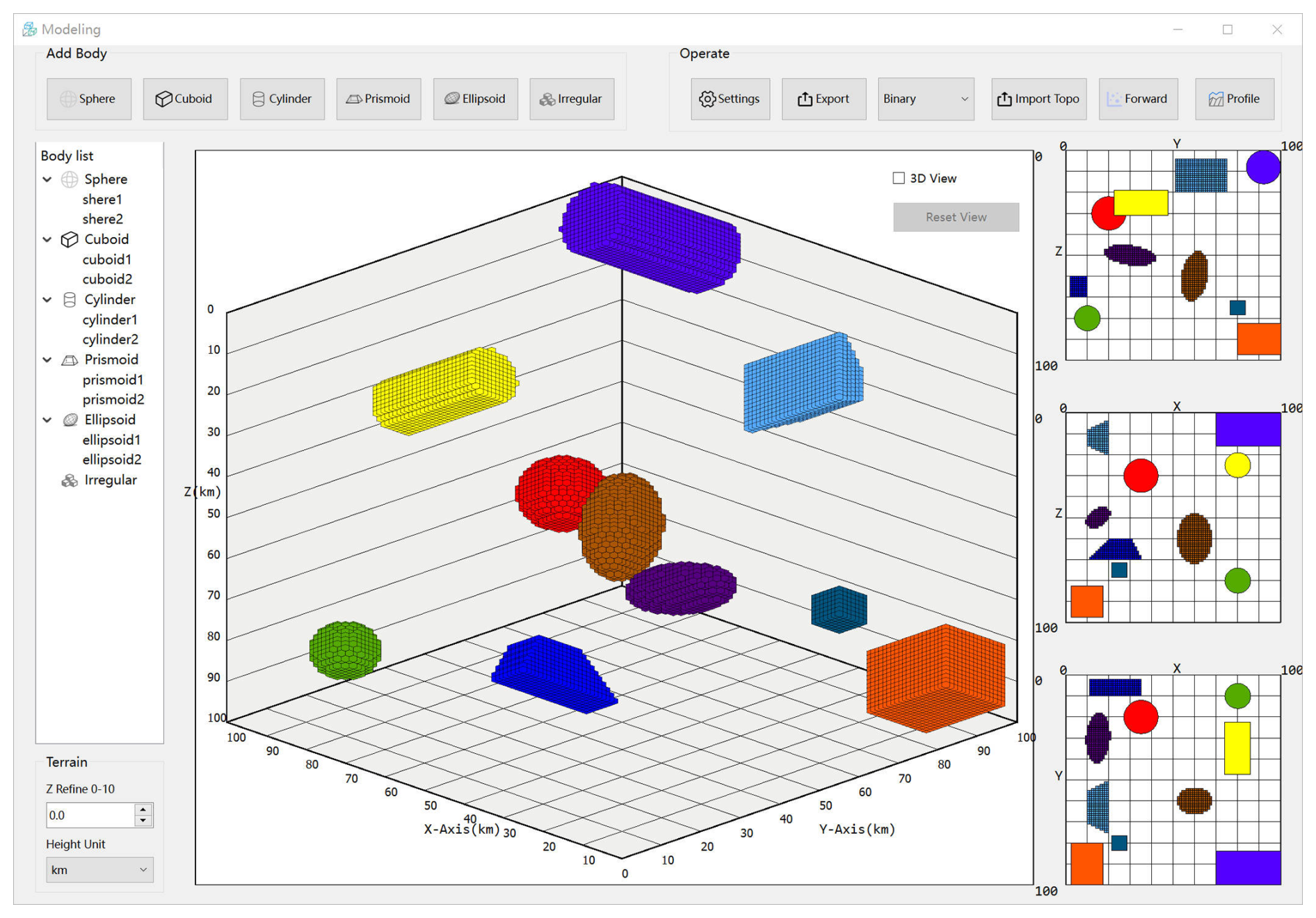
G&M3D 1.0 provides five tools for creating regular-shaped bodies: Sphere, Cuboid, Cylinder, Ellipsoid and Prismoid. Figure 6 displays the parameter input interfaces for each tool. (1) Sphere: This tool requires the radius and the coordinates of the sphere's center. (2) Cuboid: Users must input the geometric centre coordinates and the extension lengths along three orthogonal axes. (3) Cylinder: Four key parameters are needed to define a cylinder, including the trend direction, extension length, cross-sectional radius, and section centre coordinates. (4) Ellipsoid: A rotated ellipsoid is defined by the centre coordinates, the radii of the three semi-axes, and the rotation angle. (5) Prismoid: This geometry is defined by three sets of spatial parameters: the x-coordinates of its four y-parallel edges, the y-coordinates of its four x-parallel edges, and the z-values for its top and bottom planes. To enhance modelling flexibility, the “Direction” parameter specifies the normal vector orientation of the bounding planes relative to the coordinate axes. The Prismoid tool maintains strict geometric validity by enforcing essential constraints: the x-coordinates must be monotonically increasing (x1<x2), and the y-coordinates (y1<y2) likewise, ensuring proper spatial relationships for meaningful prism construction. All bodies require input of either density contrast or magnetization. Additionally, the “Mark” panel allows users to customize both the body's name and display colour according to their preferences. As an example, we create two bodies using each tool, resulting in a total of ten bodies, which are presented in Fig. 7.

Figure 7 Illustration of regular modelling tools showing ten anomalous bodies.

G&M3D 1.0 features an Irregular tool that enables users to create irregular bodies, as shown in Fig. 8. With the Irregular tool, users can accurately construct irregularly shaped bodies by interactively drawing their spatial boundaries across multiple layers. This layer-stacking method allows for the reconstruction of complex volumetric shapes that cannot be represented using conventional geometric primitives. G&M3D 1.0 automatically generates a set of prisms that fit within the limits defined by users in one layer, extending along the x, y, or z direction. To enhance operational efficiency, the software employs a dual-mode: Build Mode for creating anomalous prismatic units, and Erase Mode for removing existing anomalous units. These complementary modes work in tandem to minimize operational errors, effectively eliminating the need for complete rebuilds in case of mistakes. To maximize operational flexibility while avoiding redundant constraints, both modes maintain identical workflows and interaction processes. To facilitate reference-guided modelling, the Irregular tool also allows users to load a semi-transparent background image as a visual reference (Fig. 8).

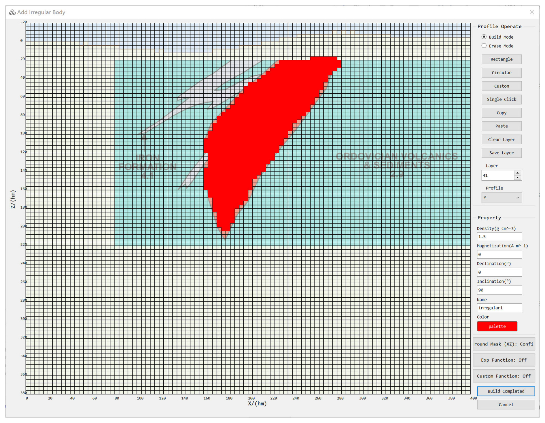
Figure 8 Interface of the Irregular tool. The main area is used to delineate the boundaries of the anomalous bodies. Right panels contain functional zones and parameter setting areas. Build Completed and Cancel buttons are used to finalize or abort the entire irregular modelling process, while all other functions only operate on the current layer. In this example, a screenshot adapted from Thomas (1997) is used as a semi-transparent background template to construct an irregular sulphide deposit with a density contrast of 1.5 g cm⁻³.

In the Irregular tool, G&M3D 1.0 offers four drawing modes: Rectangle, Circular, Custom, and Single Click. The modelling process uses a standardized left-click operation across all modes. Users press and hold the mouse button to activate a real-time visual preview of the modelling area, and release it to confirm and finalize the operation. In the Custom mode, users can draw any closed curve to define the boundary of the anomalous body, allowing automatically generated prisms to fit the boundaries more accurately with gradual sketching. To enhance workflow efficiency, G&M3D 1.0 includes Copy and Paste functionality for layers. Once users have finalized the geometric modelling and parameter settings (via the unified Property panel, consistent with regular modelling tools) for the current layer, they must manually save the layer data using the Save Layer option. After completing the model construction for all target layers, users can execute the “Build Completed” command to finalize and save the complete dataset. An example of constructing an irregular sulphide deposit model beneath undulating topography is shown in Fig. 9.

Figure 9 An irregular sulphide deposit model constructed using the Irregular tool.

Once all anomalous bodies have been constructed, G&M3D 1.0 allows users to export both the model geometry and the corresponding physical property distributions in multiple data formats. Supported export formats currently include binary, text and UBC-GIF, which can be selected directly from the drop-down menu in the Export tool. This design not only facilitates the segmentation of workflows between building source models and forward modelling tasks, potentially assigned to different operators, but also enhances operational flexibility throughout the gravity and magnetic data processing workflow. The binary .bin format efficiently retains comprehensive parametric data, while the text-based .txt export adheres to standardized formatting specifications to facilitate interdisciplinary data exchange.

G&M3D 1.0 provides two methods for forward modelling. Users can either initiate the computation through the Forward tool found in the “Operate” panel (Fig. 5) to build source models and perform forward modelling within a unified project environment or directly import the pre-constructed models into the Forward-Modelling module using the Input Model option (Fig. 4). Figure 10 shows the main interface of the Forward-Modelling module. To perform forward calculations, users must first select the desired anomalous bodies by checking the corresponding boxes in the “Body list” panel. Once the bodies are selected, users can initiate the forward modelling process by clicking the Forward Model button, which opens the Forward Model interface (Fig. 10b). In this interface, users configure the observation parameters, including observation height and optional noise levels for simulating mobile-platform gravity and magnetic surveys. In addition, users can choose whether to enable parallel computation and whether to perform the calculation with topography. After configuring these settings, clicking the ok button will execute the forward calculation. Upon completion, G&M3D 1.0 automatically generates a pseudocolor plot of the results. Users can switch between different datasets using the drop-down box. The forward modelling results can be viewed in G&M3D 1.0 or exported as datasets by clicking the Save Data button.

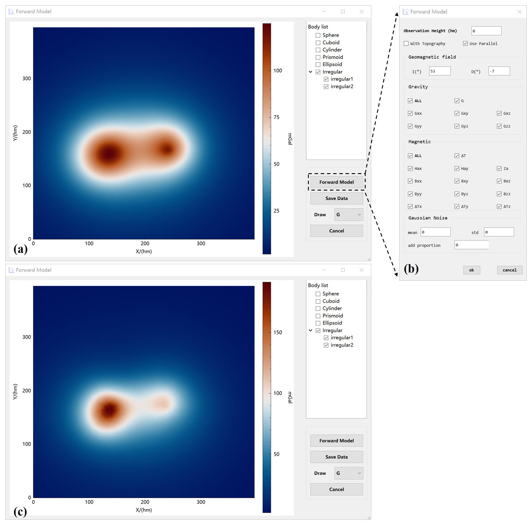
Figure 10 (a) Interface of the Forward-Modelling module. The left workspace is used to visualize the gravity/magnetic field. The upper right area shows the body list, and different bodies can be selected for forward calculation. The functional control area is located in the lower right section. A sulphide deposit is shown as an example, adapted according to Thomas (1997). (b) Parameter input pop-up window for Gravity forward modelling, Magnetic forward modelling. A certain proportion of Gaussian noise can be added to the field values to simulate errors. Mag-Inclination and Mag-Declination correspond to the inclination (I) and declination (D) of the Earth's geomagnetic field in Eqs. (17)–(20). Users can freely select the field category to be calculated. (c) Results calculated over undulating topography.

4 Application

The 3D modelling and forward calculations of the gravity and magnetic fields in G&M3D 1.0 provide practical tools for potential data analysis and interpretation. Although inversion is not implemented in the current version, the software provides flexible initial or synthetic models for studies related to inversion. Researchers often conduct synthetic model experiments to test the feasibility of their algorithms and assess parameter sensitivity. With G&M3D 1.0, they can easily create numerous density contrast or susceptibility models and quickly obtain the gravity/magnetic data. Moreover, G&M3D 1.0 serves as a practical educational resource for teaching geophysics, particularly for beginners in gravity and magnetic exploration. Educators and students can utilize G&M3D 1.0 to construct simplified geophysical models, enabling them to explore the principles of the potential fields through interactive visualization and analysis.

To illustrate the functionality of G&M3D 1.0, we perform a gravity modelling analysis of a representative salt dome as an example. This salt dome model is based on available seismic and drill-hole data from Vinton Dome in southern Louisiana (Ennen, 2012). It features a caprock with positive-density contrast at depths ranging from 160–760 m, alongside a negative-density contrast salt volume located deeper. In the study by Ennen (2012), gravity gradients produced by this salt dome model are calculated and compared to observed airborne gravity gradient data to identify potential oil signals. As highlighted by Ennen (2012), constructing such an irregular density contrast model for a salt dome is a labor-intensive process.

In this example, we utilize the salt dome model described by Ennen (2012) to demonstrate the 3-D modelling and forward calculations of gravity gradients using G&M3D 1.0. According to this study, the source space is divided into $\mathrm{66}\times \mathrm{45}\times \mathrm{28}$ prisms with dimensions of $\mathrm{100}\mathrm{m}\times \mathrm{100}\mathrm{m}\times \mathrm{100}\mathrm{m}$. The density anomaly of the salt dome varies in geometry at different depths, with differing density contrasts, as presented in Table 2.

Table 2 Density contrast distribution of the salt dome model along the depth.

Figure 11 The salt dome model built by G&M3D 1.0.

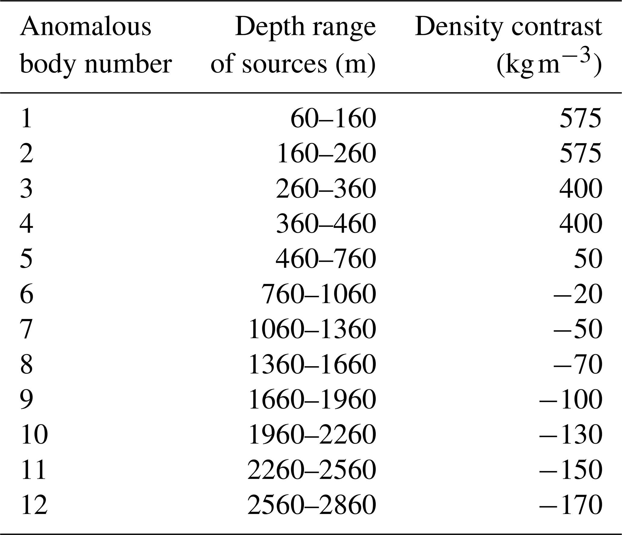
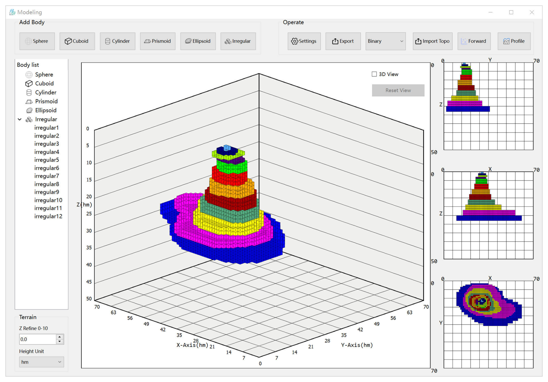
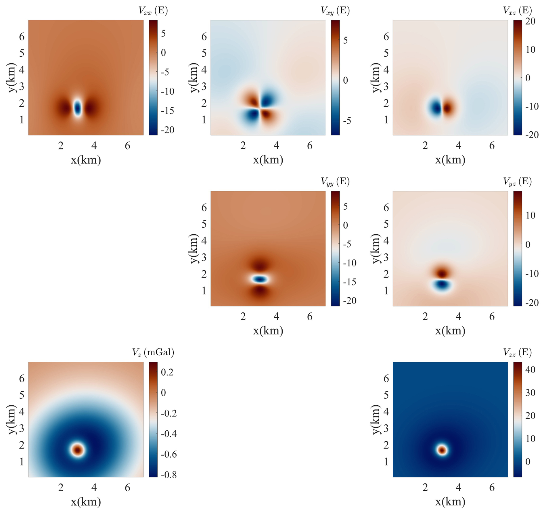
Figure 12 The gravity field and gradient components generated by the salt dome model using G&M3D 1.0. Here, $\mathrm{1}\mathrm{mGal}={\mathrm{10}}^{-\mathrm{5}}\mathrm{m}{\mathrm{s}}^{-\mathrm{2}}$ and $\mathrm{1}\mathrm{E}={\mathrm{10}}^{-\mathrm{9}}{\mathrm{s}}^{-\mathrm{2}}$.

In G&M3D 1.0, we apply the Irregular tool in the Modelling Module to create a density contrast model of the salt dome. This salt dome structure can be approximated by 12 separate irregular bodies located at different depths, each with a constant density contrast, as shown in Table 2. We build these bodies successively using the Modelling Module in G&M3D 1.0. First, we set the range for the source region in the x, y, and z axes to [0 7 km], [0 7 km], and [0 5 km], respectively. The division step is set to be $\mathrm{100}\mathrm{m}\times \mathrm{100}\mathrm{m}\times \mathrm{100}\mathrm{m}$. Next, in the Layer-Building interface, we specify the layer number as 28 and the density contrast as $-\mathrm{170}\mathrm{kg}{\mathrm{m}}^{{-}^{\mathrm{3}}}$. Using Custom mode, we outline the geometry of the salt dome at this depth in the workspace, and then we use Single Click mode to make slight modifications to its shape. After making these modifications, we save this anomalous body and change the layer number to 27. The copy and paste functions allow us to visualize the source geometry from the previous layer on the interface, which facilitates anomaly source localization. Users can easily modify the existing layer structure, significantly improving modelling efficiency. This process can be repeated to quickly build the complete salt dome model (Fig. 11).

After constructing the 12 anomalous bodies that form the salt dome model, we use the Forward Modelling Module to calculate the gravity fields and gradients. We set the observation range to match that of the source, with the observation height fixed at 200 m. The resulting gravity fields and gradient components are shown in Fig. 12. To validate the accuracy of G&M3D 1.0, we conduct a comparative analysis with spatial domain approaches (Li and Chouteau, 1998). The maximum absolute difference is $\mathrm{1.2}\times {\mathrm{10}}^{-\mathrm{12}}\mathrm{mGal}$ for the gravity anomaly and $\mathrm{1.3}\times {\mathrm{10}}^{-\mathrm{12}}\mathrm{E}$ for the gravity-gradient components. These data are consistent with the forward simulation results provided by Ennen (2012), confirming the accuracy of the forward calculation in G&M3D 1.0.

5 Conclusions

The study introduces an open-source software called G&M3D 1.0, developed using the Qt application framework and C++ programming language. G&M3D 1.0 is designed to create 3D models of density contrast and magnetization, as well as to compute their gravity and magnetic fields. Users can run the software either from source code or as a standalone desktop application. With G&M3D 1.0, users can easily create arbitrary anomalous bodies and perform modifications, deletions, storage, and display of the model. Furthermore, G&M3D 1.0 extends the efficient BCE algorithm for forward calculations of gravity gradient tensors and magnetic gradient tensors. Lastly, we demonstrate the gravity modelling over the Vinton salt dome in southern Louisiana, U.S. This practical application illustrates how G&M3D 1.0 can be utilized for geophysical research, training, data processing and interpretation. The modular architecture of G&M3D 1.0 also provides a robust foundation for future extensions, including incorporating additional body types, more flexible property representations, and advanced new forward functions.