Composite sharpening by vortex symmetrization and normalization of tropical cyclones

Cyclone composites are a powerful tool for investigating the mean characteristics of tropical cyclones (TCs), offering insights into the mechanisms driving storm development. Traditional composite methods align cyclone centers to capture large-scale patterns but they tend to smooth out mesoscale features.

We introduce a novel compositing framework, the SYmmetrized-Normalized Cyclone (SyNC) compositing, designed to address the structural variety of TCs. This method symmetrizes storms to axisymmetric vortices and normalizes them according to their eyewall location and the size of the TC (defined by the radius of 17 m s⁻¹ winds). The method is applied to simulated TCs with the weather and climate model ICON run at 5 km horizontal grid length. ICON reveals the ability to simulate even most intense storms, while overestimating the frequency of major hurricanes and underestimating the seasonal TC frequency.

By asymmetrically detecting the eyewalls and the horizontal extents of TCs, the SyNC method enables detailed storm structural analysis. A large structural variability and asymmetries are found across all simulated storm intensities, agreeing with observations.

The eyewall alignment of the SyNC framework successfully sharpens composite fields, preserving extreme values of mesoscale features such as super-gradient winds, eyewall updrafts, eyewall precipitation, and localized latent heating related to cloud microphysics. It also reduces within-group variance, thereby increasing statistical power and enabling the detection of differences between TC groups that would be missed using traditional center-based compositing. Limitations of the SyNC composites include reduced applicability during early storm stages, when tangential winds have not yet formed a Rankine-like vortex, and potential data extrapolation during normalization in small storms. Nonetheless, the method proves robust for weakly organized storms. SyNC is particularly beneficial for analyzing mesoscale features using high-resolution data (horizontal grid length of ≈ 10–20 km or finer) capable of resolving these features as well as the structural variability of TCs. As numerical models continue to improve in resolution and representation of mesoscale features and vortex variability, TC misalignment in composites will likely become an increasing challenge. Overall, the SyNC compositing method provides a cyclone-relative framework that improves the accuracy of TC composite analysis, thereby facilitating the investigation and understanding of storm development.

1 Introduction

Cyclone composites are widely used to analyze mean characteristics of groups of tropical cyclones (TCs) to improve the understanding of their development and structure (Klotz and Jiang, 2017; Bengtsson et al., 2007; Wei et al., 2025; Sun et al., 2019; Ming et al., 2015; Trier et al., 2023). Cyclone composites are usually calculated by taking the average of a cyclone group at a particular stage of their life cycles after aligning the cyclone centers (Bengtsson et al., 2007; Hanley et al., 2001; Trier et al., 2023). Some composite methods project each cyclone to the Equator, thereby using great-circle distances to represent cyclone size to make cyclones located at different latitudes more comparable (Vessey et al., 2022). To better preserve their key structures, TCs are sometimes rotated according to their storm motion or to the environmental vertical wind shear (VWS) (Klotz and Jiang, 2017; Rios-Berrios and Torn, 2017; Uhlhorn et al., 2014; Zhang et al., 2013; Carstens et al., 2024). Storm motion increases the tangential wind field asymmetry by contributing to the wind speed where the storm's tangential wind vectors and translation vectors align, typically on the right side of the storm track (Uhlhorn et al., 2014). VWS influences the storm structure by increasing the tangential and radial wind asymmetry (Klotz and Jiang, 2017; Carstens et al., 2024) and is associated with asymmetric surface fluxes and asymmetric convection (Zhang et al., 2013; Carstens et al., 2024; Rios-Berrios et al., 2024). However, depending on the research focus, TC composites can also not be rotated, when for example studying the interactions with upper-tropospheric troughs (Hanley et al., 2001). Generally, cyclone composites capture persistent synoptic scale patterns well but tend to smooth out smaller scale features (Bengtsson et al., 2007, 2009; Binder et al., 2016; Dacre et al., 2012; Vessey et al., 2022). The smoothing of mesoscale features within cyclones can be caused by misalignment of the storm's structures, when the compositing TC group contains various storm sizes and vortex axis-asymmetries, while only aligning the TC centers.

To which extent vortex structures and mesoscale features are represented in numerical models depends strongly on their horizontal resolution: In models with horizontal grid length of ≈ 25–250 km, mesoscale precipitation features for example are not resolved, leading to radially smoother and more homogeneous precipitation patterns (Sena et al., 2024; Zhang et al., 2021). Using a smaller horizontal grid length of ≈ 20 km and finer allows for a better representation of mesoscale convection, thereby increasing spatial variability in precipitation and bringing simulated precipitation fields closer to observations (Chen et al., 2007). A similar resolution dependence is found for tangential winds: at coarse resolution (horizontal grid length of ≈ 100 km), the wind field is relatively smooth, whereas pronounced horizontal variability in wind emerges at horizontal grid length of around ≈ 10 km or finer (Manganello et al., 2012; Judt et al., 2021).

Indeed, observed TCs reveal various vortex sizes and are rarely geometrically axisymmetric vortices. The vortex size is often defined as the radius where the wind field reaches 17 m s⁻¹ (R17, Kepert, 2010; Chan and Chan, 2012; Judt et al., 2021). R17 of North Atlantic TCs ranges from 101 to 370 km (10th–90th percentile). The radii of maximum winds (RMWs) of North Atlantic TCs have a 10th–90th percentile range of 28 to 111 km (Chan and Chan, 2012). The deviation from a perfect circular vortex is often measured by an asymmetry index (AI), which synthesizes measured wind radii in each quadrant around the TCs center (Chan et al., 2023). Chan et al. (2023) analyzed AIs of different sizes and found that TCs are rarely symmetric in all basins and highlighted the limitation of taking azimuthal average wind fields to quantify storm sizes.

Misalignment of eyewall and TC borders can lead to a loss of information of key physical processes that are critical for understanding storm development and associated hazards, as these processes are tightly linked to the vortex structure: RMW is often an approximation of the eyewall location (Kepert, 2010; Qin et al., 2016). In the eyewall, cloud microphysical processes and associated latent heating are indicative of warm core formation (Ohno and Satoh, 2015). Strong vertical velocities in the eyewall provide insight into the intensity of the secondary circulation (Kepert, 2010; Smith and Montgomery, 2023). Rainbands are mainly found within and around the storm border (i.e., R17). Also most of the precipitation falls within R17 (Yu et al., 2023). Some studies suggest competing effects of rainband and eyewall convection due to aerosol-cloud interactions in TCs (Lin et al., 2023; Wang et al., 2014; Rosenfeld et al., 2012), which gives another reason to preserve both, eyewall and outer rainbands, as well as make them distinguishable from each other. Besides analyzing features linked to the vortex structure, size, RMW and AI themselves can be useful parameters in studying the evolution of storms and their impact on coastal regions: determining the precise size of a TC can improve the estimation of its destructiveness potential (Emanuel, 1999). RMW is observed to contract during TC intensification due to absolute angular momentum convergence by the overturning circulation, and can coincide with or precede rapid intensification (Stern et al., 2015; Qin et al., 2016), an ongoing challenge in TC forecasting (Zhang and Tao, 2013). Relatively symmetric storms also have larger intensification rates, likely due to the absence of VWS (Li and Tang, 2025). Moreover, symmetric eyewalls can benefit intensification, since they are associated with higher convective organization and larger radial heating gradients (Martinez et al., 2022; Persing et al., 2013).

Some studies tackle the challenge of various vortex structures partially by scaling the storm distances by RMW. These composite methods (Wei et al., 2025; Klotz and Jiang, 2017; Sun et al., 2019; Ming et al., 2015) allow the alignment of eyewalls, within the compositing storm group. Nevertheless, the various vortex sizes and asymmetries are not considered in such an approach.

As numerical models achieve finer resolutions and more accurately capture mesoscale features and vortex variability, the challenge of TC misalignment in composites will likely become increasingly relevant. This study presents a novel approach to composite TCs addressing their large spread in vortex sizes and axis-asymmetries: the SYmmetrized-Normalized Cyclone (SyNC) composite framework aims to symmetrize TCs to axisymmetric storms and normalize them according to their eyewall location and storm border to preserve the individual storm structures and associated features when compositing cyclone groups with various asymmetries and sizes. It further presents an approach to accurately detect the vortex and eyewall sizes, as well as corresponding axis-asymmetries. We developed the method on a group of numerically simulated TCs and compare their characteristics and structure to the HURDAT2 best track dataset (Landsea and Franklin, 2013).

This manuscript first presents the methodology (Sect. 2) including the ICON model setup and TC tracking. A detailed technical description of the SyNC processing steps is presented in Sect. 2.6. Section 3 validates the simulated TC dataset against best track data to estimate its realism and representativeness for other TC datasets thereby indicating the broader applicability of SyNC to other datasets. To assess the SyNC approach, two case studies illustrate the effects of vortex symmetrization and normalization on individual vortices (Sect. 4). Section 5 analyzes the structural evolution of simulated and observed TCs exploiting the fine detection of simulated RMW, R_out, their AIs, and eyewall tilt by SyNC. Finally, Sect. 6 compares the SyNC composites with composites conducted by only aligning the TC centers to evaluate the performance of SyNC and identify its benefits and limitations.

2 Methods

2.1 Model setup

For the development and demonstration of the SyNC composites, the North Atlantic TC season 2005 was simulated using the non-hydrostatic numerical weather prediction and climate model ICON (Zängl et al., 2015, ICON partnership (DWD; MPI-M; DKRZ; KIT; C2SM) (2024). ICON release 2024.10. World Data Center for Climate (WDCC) at DKRZ) in limited area mode. The model domain spans the North Atlantic ocean (5 to 45° N, 105 to 18° W) using a triangular grid with 5 km (grid R2B9) horizontal grid length, 80 vertical levels up to 23 km and a time step of 25 s. Initial and six-hourly boundary conditions were taken from ECMWF IFS HRES analysis product. Sea surface temperature was prescribed using daily fields online-interpolated from monthly mean input, itself derived from the ECMWF 6-hourly IFS HRES analysis for 2005. Simulations ran from 1 July to 1 December 2005, including a two week spin-up. The selected months were chosen to capture the climatological peak of hurricane activity while balancing computational cost. The model physics is represented by a set of parametrisations: the prognostic turbulent kinetic energy (TKE) scheme for turbulences (Raschendorfer, 2001), the ecRad scheme for radiation (Hogan and Bozzo, 2018), the TERRA scheme for land surface processes (Schulz et al., 2016) and the two-moment scheme of Seifert and Beheng (2006) for clouds, predicting mass and number concentrations of cloud droplets, ice crystals, rain, snow, graupel and hail. Cloud droplets' growth is implemented by saturation adjustment, whereby updraft-induced water vapor supersaturation is reduced to 100 % by condensation on cloud droplets. Cloud droplets are formed by the cloud condensation nuclei (CCN) activation scheme of Segal and Khain (2006). The CCN concentration is prescribed to 500 cm⁻³ representing average conditions over the North Atlantic (Choudhury and Tesche, 2023). Deep and shallow convection parametrisations are switched off to align our setup with convection-permitting ICON studies from Hohenegger et al. (2023), Weiss et al. (2025) and Segura et al. (2025). Hohenegger et al. (2020) showed, that ICON is able to sufficiently capture the water and energy budgets, the cloud distribution in the tropics and the location of the InterTropical Convergence Zone (ITCZ) and hence is able to reproduce key features of the climate system without convection parametrisations at 5 km. Additionally, Judt et al. (2021) demonstrated that both simulated TC numbers and Accumulated Cyclone Energy (ACE) in ICON are much closer to observational values when the deep convection parametrization is switched off.

2.2 Ensemble generation

An ensemble of eight members was computed to increase the TC group size and assess the internal variability in the simulations. Ensemble members were created according to the method described by Fischer et al. (2023) by perturbing the initial specific moisture field. Random perturbations on the order of a rounding error ($\pm {\mathrm{10}}^{-\mathrm{13}}$ kg kg⁻¹) were added to the initial moisture field. The initially small perturbations grew as the simulations proceeded. Since the model is only constrained by the 2005 large-scale environment at the lateral domain boundaries, each member has some degree of freedom to evolve into its own internal state within the domain. Consequently, the simulations represent eight plausible realizations of the 2005 season rather than its exact reproduction. The simulated TC tracks therefore diverge from observed tracks (Fig. A1 in Appendix A).

2.3 TC tracker

TCs were identified using the multi-parameter TC tracking algorithm of Enz et al. (2023). The algorithm employs three typical TC characteristics: a surface pressure depression, a cyclonic wind field and a warm core located in the upper troposphere. These characteristics are detected by the algorithm at each time step using four parameters, each evaluated across multiple threshold values (shown in parentheses):

• 1.

  A local sea level pressure minimum within a given distance (p_min, dist [50, 100, 150] in km).

• 2.

  High relative vorticity detected at ≈ 2.5 km altitude (ζ_min [$\mathrm{1}\times {\mathrm{10}}^{-\mathrm{6}}$, $\mathrm{1}\times {\mathrm{10}}^{-\mathrm{5}}$] in s⁻¹).

• 3.

  A temperature anomaly at 300 hPa (ΔT_core [0.5, 0.75, 1.0, 1.25, 1.5] in K) within a given distance (T_dist [50, 100, 200, 300, 400] in km).

Thresholds for the parameters follow the original implementation of Enz et al. (2023) and were selected based on scientific literature and physical feasibility. In total, 150 threshold combinations are possible, whereof weak/strong TCs fulfill a low/high number of threshold combinations, respectively. A system is classified as a tropical depression once at least 10 % of the threshold combinations are met, which defines the start and end points of the detected TC tracks. The TC center is identified by the sea level pressure minimum. Once a TC center is identified at time step t₀, it is linked to the nearest TC center found at t₋₁, whereby a maximum translation velocity threshold of 25 m s⁻¹ is applied. As shown by Enz et al. (2023), the tracker identifies systems once they reach tropical depression strength. Track termination is primarily associated with the loss of the warm core or excessively high translation speeds in the extratropics (for more detail see Enz et al., 2023).

2.4 TC filtering

After cyclone detection, simulated TCs were filtered to exclude weak and short-lived systems based on the following criteria: minimum lifetime of 48 h and reaching a minimum central pressure (p_min) of 990 hPa or lower. We employed the pressure based intensity scale by Klotzbach et al. (2020), which covers pressure categories (cat_pres) from 1–5 starting at a pressure of ≤ 990 hPa being cat_pres of 1. The pressure based intensity scale has multiple benefits: pressure measurements are more accurate than wind measurements, p_min is a strong indicator of potential damage (Klotzbach et al., 2020) and the climatological spread in pressure distribution is better captured by numerical models than for maximum winds (Knutson et al., 2015; Bourdin et al., 2024; Manganello et al., 2012). The wind-pressure relationship of TCs is poorly represented in numerical models often revealing too weak winds for a given central pressure with increasing error towards intense TCs (Bourdin et al., 2024; Judt et al., 2021; Knutson et al., 2015; Reed et al., 2015; Bao et al., 2012; Manganello et al., 2012). In climate models with horizontal grid lengths of ≈ 20–200 km, the simulated wind-pressure relationship improves with increasing resolution by better resolving the vortex leading to a more realistic representation of its structure and the development of intense tropical cyclones (Cat 3–5; Bourdin et al., 2024; Manganello et al., 2012; Davis, 2018). Storm-resolving models operating at approximately ≈ 2–10 km horizontal grid length further improve simulated storm structure and intensity compared to coarser-resolution models, although model-dependent biases remain (Chen et al., 2007; Judt et al., 2021; Baker et al., 2024). Possible sources of this model dependence include the choice of dynamical core (Reed et al., 2015) and the model's physics parametrization, which determine the surface drag in the boundary layer and diabatic heating through cloud processes and by that influence the simulated TC intensities and structures (Bao et al., 2012; Baker et al., 2024). Accordingly, pressure-based metrics are more robust and well-suited for analyzing TC activity in numerical models, as demonstrated in the study by Bourdin et al. (2024).

2.5 Time normalization

To enable meaningful comparisons between TCs with different lifetimes, the evolution of each storm is normalized, inspired by the method of Schemm et al. (2018). The time axis is rescaled to an interval of [0, 1], where t_norm = 0 corresponds to genesis, t_norm = 0.5 to the time of minimum central pressure (i.e., maximum intensity), and t_norm = 1 to storm lysis. Between these three fix points, the normalized time axis is linearly interpolated to the tracking time steps. Accordingly, the intensification phase spans from t_norm ∈ [0, 0.5] and the decay phase from t_norm ∈ [0.5, 1]. TC genesis and lysis are defined by the start and end points of the detected TC tracks.

2.6 SyNC: Symmetrized-Normalized Cyclone composites

The goal of the SYmmetrized-Normalized cyclone (SyNC) composite approach is to reduce composite blurring from misaligned vortex structures. Each TC is transformed to an axisymmetric vortex and spatially normalized based on the eyewall radius and the storm size. That way, eyewalls and storm borders are aligned when compositing the symmetrized-normalized TCs. In this section, all processing steps of SyNC are described in detail. There are four main steps to obtain SyNC composites (see Table 1):

• 1.

  Cyclone-centered projection of the TC from a sphere to a plane.

• 2.

  Sector-wise eyewall and storm border detection.

• 3.

  Vortex symmetrization and normalization.

• 4.

  Compositing data fields of a TC group.

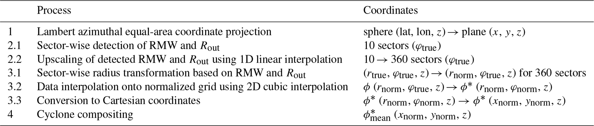
Table 1 Steps to obtain the symmetrized-normalized TC composites and corresponding coordinate conversions. The geographic coordinate system is defined by the coordinates latitude lat, longitude lon and height z. The cartesian coordinate system spans over the horizontal plane with x and y with the vertical coordinate z. The cylindrical coordinate system is described by the radial distance to the TC center r, the azimuth φ and height z. The subscript true refers to the real cylindrical coordinate system, while the subscript norm indicates the normalized cylindrical coordinate system. ϕ represent any three-dimensional data field of one TC, ϕ^* the data field after interpolation and ${\mathit{\varphi }}_{\mathrm{mean}}^{*}$ the data field mean over a group of cyclones.

First, each TC is projected from the Earth's sphere to a plane using a cyclone-centered Lambert azimuthal equal-area projection. This creates a Cartesian grid (x, y, z) with the grid origin located at the cyclone center addressing the irregular spacing of the grid due to the curvature of the Earth. Therefore, the projected grid preserves the true size of a cyclone and enables the comparison of cyclones across different latitudes. The projected horizontal grid length is set to match the model grid length (Δx=5 km) to avoid data extrapolation or interpolation, thereby minimizing data modification in this initial step. Additionally, the model output is reduced to a 1000 km × 1000 km square around the TC center to speed up the post-processing. This defines the extent of the data and determines R_max.

Second, the eyewall and the storm's size are detected based on the tangential wind field (see Fig. 1a). The location of the eyewall is approximated by RMW (Kepert, 2010; Qin et al., 2016). The horizontal extent of the TC is defined as the radius where the wind speed reaches 17 m s⁻¹ (Kepert, 2010; Chan and Chan, 2012; Judt et al., 2021, R17, from now referred to as R_out). RMW is identified for each vertical level, what allows to further estimate the eyewall tilt. When the tangential wind becomes anticyclonic at upper-levels, RMW is taken from the last level below, where winds are still cyclonic. R_out is detected from the tangential wind mean between the surface and 2 km. This ensures better representation of the storm size compared to detecting R_out only at a single vertical level. The 2 km level was selected, since it leads to the largest TC extents and with that conservatively keeps most of the vortex data in the analysis (find more details and a sensitivity experiment in Appendix B1). R_out is maintained for all height levels. Otherwise, the anticyclonic outflow would unrealistically narrow the vortex size at upper-levels. Note that the cyclone center is defined as the location of the sea level pressure minimum and is assumed not to vary with height. This assumption can introduce errors in radial and tangential wind components in the presence of vortex tilt, particularly at upper levels. However, errors mainly affect radial winds, while tangential winds are only weakly impacted (Ryglicki and Hart, 2015). Therefore, the wind radii detection are not expected to be strongly affected by this simplification. To make the wind radii detection robust, some additional rules are implemented: RMW is forced to a minimum/maximum of 15 km/400 km and R_out is capped at a maximum of 700 km. In case of a narrow R_out-RMW ring, R_out is increased until a minimum distance of 30 km between RMW and R_out is fulfilled to avoid extensive extrapolation of data points in case of a narrow R_out-RMW ring. Additionally, to exclude detected extreme radii, detected RMW and R_out are excluded when exceeding 300 % or 600 % of the median of this level, respectively, and replaced with a rolling average of radii in their neighboring sectors. These thresholds were selected based on statistics of observed wind radii and R_out-RMW distances. During testing of the algorithm, the thresholds were rounded and adjusted to the simulated TC structure in such a way that the thresholds were only applied when physical radius detection would not have been possible without them. The thresholds are especially necessary for obtaining feasible radii in the early stage of a TC, where the vortex structure is less pronounced and above 15 km, where the vortex ends or the anticyclonic outflow complicates the radii detection. For more details about threshold selection and when they are applied see Sect. B3. The RMW and R_out detection is done for 10 circle sectors (i.e., 36° sectors) individually around the cyclone center to account for vortex asymmetry (Fig. 1a). The detection resolution of 36° was chosen such that each sector contains at least one grid cell within the detection minimum of RMW (illustrated in Fig. B3b in Appendix B), which is a necessary condition to detect RMW for each sector. Hence, the maximum number of detection sectors is dependent on the data resolution, whereof for higher resolution, also a higher number of detection sectors can be employed. A high number of detection sectors can improve the detection of vortex asymmetries, as shown by a sensitivity experiment of AI to the number of detection sectors (Sect. B2). These findings suggest that the highest feasible number of detection sectors should be selected. The 10 detected R_out values are smoothed by a rolling mean over 3 data points to avoid spikes in the TC size. After this, the resolution of detected RMW and R_out is increased by linearly interpolating the detected radii from 36° sectors to 1° sectors (Fig. 1b). This allows for a more continuous vortex normalization in the next step.

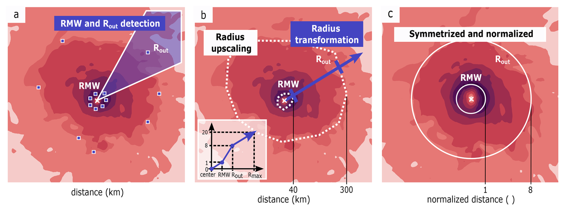
Figure 1 Illustration of the process steps to symmetrize and normalize TCs. Sector-wise RMW and R_out detection (a, visualizing step 2.1 in Table 1). The purple squares indicate the detected radii, while the purple shaded area highlights one detection sector. Upscaled detected radii (dashed white circles, step 2.2 in Table 1) and sector-wise radius transformation (purple arrow) by a linear function converts real radii to a normalized radii, sketched by the function in the left lower corner of the panel (b, step 3.1 in Table 1). A symmetrized-normalized TC on the normalized grid (c, step 3.2–3.3 in Table 1). The red contours in (a)–(c) illustrate an exemplary tangential wind field of a TC.

The spatial normalization is conducted such that the TC center is located at the grid origin, while the storm's eyewall/edge are forced to a normalized radius of $\mathrm{1}/\mathrm{8}$, respectively (Fig. 1b). The normalized radii of 1 and 8 are chosen to approximately preserve the ratio between the RMW and R_out of the simulated TCs, thereby minimizing data loss and extrapolation during storm normalization. The initial sensitivity analysis (Sect. B) revealed that both RMW and R_out vary substantially within the simulated TCs. Near maximum intensity, simulated RMW values are approximately ≈ 30–50 km, while R_out is about ≈ 350 km, yielding RMW $/$ R_out ratios between 6 and 11. To account for this structural variability while maintaining a representative normalization, an intermediate ratio of $\mathrm{1}/\mathrm{8}$ was selected. Observed North Atlantic TCs exhibit a smaller RMW $/$ R_out ratio of ≈ 1 : 5 (see observed radii in Fig. B2 in Appendix B), indicating that the choice of ratio is dataset-dependent and may require adjustment when applied to other TC datasets.

The radial normalization of the cyclone is employed in cylindrical coordinates (x, y, z → r_true, φ_true, z). Based on the eyewall and border distance to the origin (r_true), a one dimensional linear interpolation function is defined, that transforms the real radius to the unit-less normalized radius (r_norm) by assigning RMW a value of 1, R_out a value of 8 and R_max a value of 20 (r_true → r_norm). Hence, each grid cell of the projected grid obtains a new normalized radius while preserving the angles (r_true, φ_true, z → r_norm, φ_true, z). The normalization is done for each of the 1° sectors individually, which forces any TC to be an approximately axisymmetric vortex. After the radius transformation, any data field (ϕ) can be interpolated from the transformed grid to a normalized grid by applying 2D cubic interpolation (ϕ (r_norm, φ_true, z) → ϕ^* (r_norm, φ_norm, z), Fig. 1c). Note that the radius transformation and data interpolation are conducted for each height level, hence the full three dimensional fields of the TCs are symmetrized and normalized. This also straightens the eyewall, which is necessary to consistently align the eyewall and its associated cloud structures throughout the vortex. Such alignment can be beneficial for investigating processes within the eyewall, such as cloud microphysics and the associated latent heating (further discussed in Sect. 6.1 and 6.2). Last, the normalized grid is converted from cylindrical to Cartesian coordinates, from which SyNC composites are calculated.

2.7 Asymmetry index

The asymmetry index (AI) is calculated to assess the vortex shapes of the different cyclone groups and to estimate the relevance of the vortex symmetrization. The AI is defined as the ratio of the maximum radius to the effective radius of four quadrants (Chan et al., 2023). Here, we calculate AI for the overall storm using R_out and for the eyewall using RMW. Instead of estimating asymmetry based on four quadrants, all detection sectors ($s_{\mathrm{1}},s_{\mathrm{2}},\mathrm{\dots },s_n$) are used, such that AI is defined as the following:

$$\begin{array}{}\text{(1)}& {\displaystyle }{R}_{max}=max(R_{s_{\mathrm{1}}},R_{s_{\mathrm{2}}},\mathrm{\dots }{R}_{s_n})\text{(2)}& {\displaystyle }{R}_{\mathrm{eff}}=\sqrt{{\displaystyle \frac{\sum _{i=\mathrm{1}}^n{R}_{s_i}^{\mathrm{2}}}{n}}}\text{(3)}& {\displaystyle }\mathrm{AI}={\displaystyle \frac{R_{max}}{R_{\mathrm{eff}}}}-\mathrm{1}\end{array}$$

where R is the detected R_out or RMW in the tangential wind field for each vertical model level, i the sector index and n the total number of detection sectors. Hence, AI of 0 indicates a perfectly symmetric structure.

2.8 Statistical significance

To assess the significance of differences between cyclone groups, we employ independent two-sided permutation tests. The test statistic is the group mean, with the null hypothesis stating that the means of the cyclone groups are equal. By randomly drawing cyclone fields from the two groups, synthetic cyclone groups are generated. This process is repeated 10 000 times. The distribution of the synthetic group means is then used to estimate the confidence interval for the null hypothesis (Wilks, 2011). The null hypothesis is rejected at a significance level of 0.05.

The permutation tests are conducted for each grid cell in the azimuthally averaged composites. To correct for multiple testing along the radius- and height-axis, and the associated risk of falsely rejecting the null hypothesis (Ventura et al., 2004), we tighten the statistics by controlling the false discovery rate (FDR) at a level of 0.05, applying the method of Benjamini and Hochberg (1995).

2.9 Best track dataset

The simulated TCs are validated by comparing their characteristics with observed cyclones from the HURDAT2 best track dataset (Landsea and Franklin, 2013). HURDAT2 is a post-storm data reanalysis of satellite, aircraft and weather station measurements and provides best estimates of North Atlantic TC tracks, central pressure and peak winds. To be consistent, observed TCs were filtered with the same criteria as the simulated TCs regarding their lifetime and minimum pressure. In addition, only storms that developed between 15 July and 1 December were considered, consistent with the chosen simulation period.

3 Simulated TC validation

3.1 Wind-pressure relationship

To evaluate the ICON-simulated TCs, the relationship between simulated wind and central pressure is compared to observations in Fig. 2. The simulated wind-pressure relationship displays a bias near the model surface (Fig. 2a–b), where most simulated 10 m winds are weaker than observed winds for a given central pressure. This suggests a model bias that may be related to the surface drag parameterization. As discussed in Sect. 2.4, such behavior is commonly found in numerical models across a range of horizontal resolutions (Bao et al., 2012; Bourdin et al., 2024; Judt et al., 2021; Knutson et al., 2015; Reed et al., 2015; Bao et al., 2012; Manganello et al., 2012). To minimize the influence of surface parameterization, a model level is identified where the wind-pressure relationship aligns well with observations for two reasons: First, it provides a wind-based intensity estimate for simulated TCs that is consistent with simulated pressure-based estimates (see Sect. 3.2), exploiting the higher confidence in the simulated central pressure. Second, it enables a comparison of wind magnitudes and wind field structures between model and observations (see Sect. 3.3) while accepting and excluding model biases near the surface. Indeed, the fit improves at higher altitudes until 0.13 km (Fig. 2c), where the best fits is located with a MSE of only 9 m² s⁻². Above 0.13 km, TC winds appear too strong for a given central pressure. Therefore, the 0.13 km level is selected for further comparisons between observed and simulated wind fields in following sections, as it offers the best alignment with observations while also being rather close to the surface. Notably, the model reproduces intense stages of TCs accurately, covering the observed range of high winds and low pressures, although it slightly under-represents weaker stages (i.e., high central pressures). The TC tracker likely struggles to detect the weak and very early stages of TCs, when the storm's central pressure is close to the ambient pressure (Enz et al., 2023). As a result, these stages are missed in our analysis.

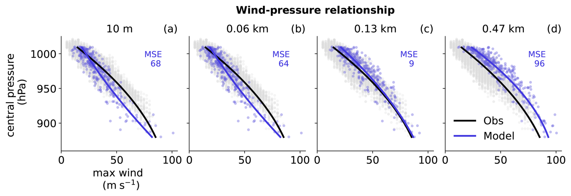
Figure 2 Wind-pressure relationship across TC life cycles for observations (black, n = 12 318) and model (blue, n = 363). Observed winds are at 10 m, modeled winds are selected from 10 m to 0.47 km (a–d). Curves show a quadratic fits excluding outliers. The mean squared error (MSE, in m² s⁻²) of the model fit is indicated in each panel.

3.2 TC characteristics

In order to place the simulated TC life cycles, frequencies and intensities into context, key TC characteristics of the simulated TCs (Fig. 3, blue) are compared to characteristics of the North Atlantic climatology (HURDAT2, 1980–2024, black) and the observed 2005 hurricane season (red). As discussed in Sect. 2.2, the simulated dataset represents plausible realizations of the highly active 2005 hurricane season. Consequently, the simulated activity is not expected to exactly reproduce the observed 2005 season nor to correspond to the climatological mean. Nevertheless, the simulated lifetime and month of genesis (Fig. 3d and h) show good agreement with the observed 2005 season and climatology. Simulated TCs predominantly form between August and October, aligning with the observed peak TC activity (Fig. 3h). However, the model fails to generate TCs during the late months of the North Atlantic TC season (November). On average, simulated TCs last approximately eight days (Fig. 3d), consistent with observed behavior. A comparison of storm tracks and additional intensification metrics can be found in Sect. A.

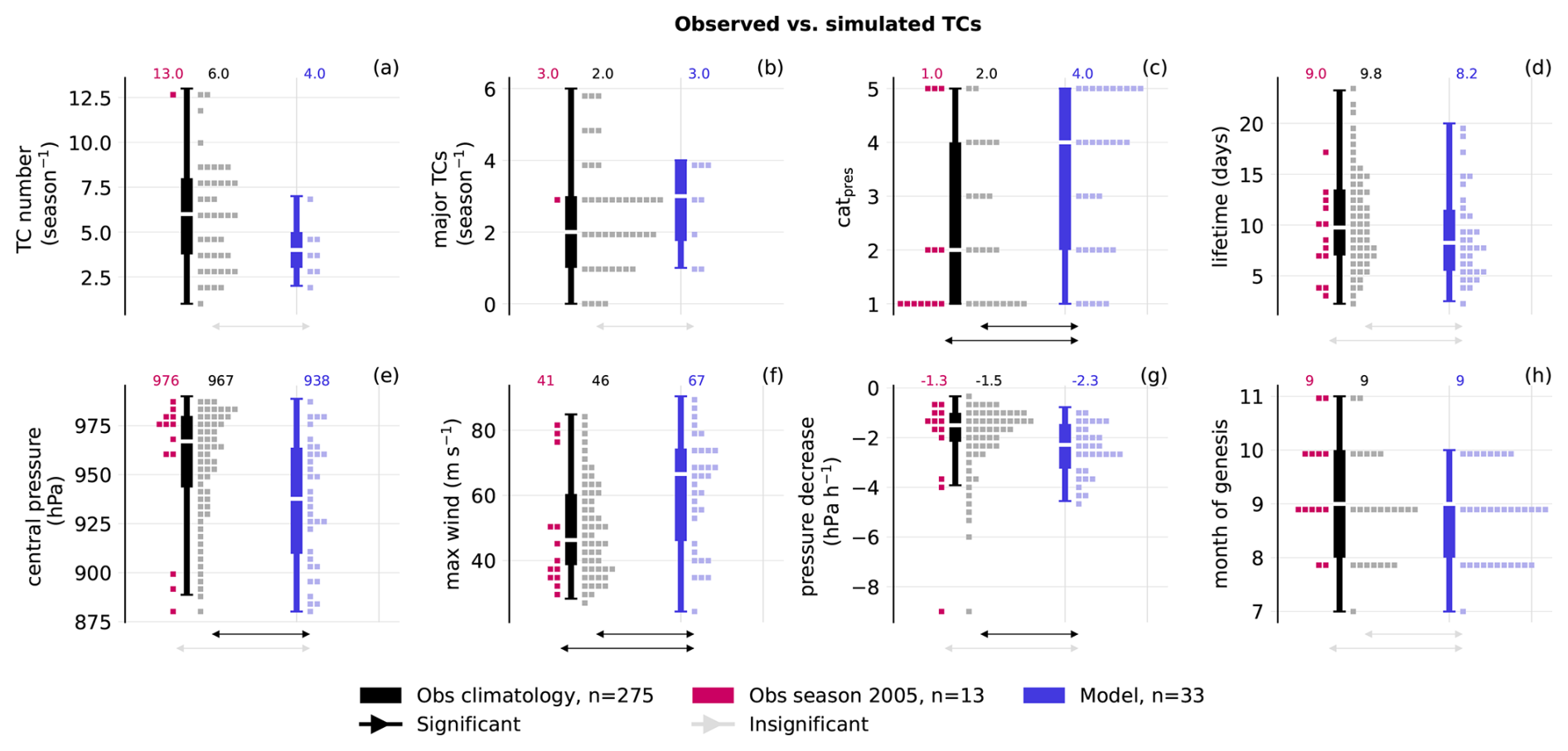
Figure 3 Comparison of observed and simulated TC activity: number of TCs per season (a), number of major hurricanes per season (cat_pres 3–5, b), overall distribution of pressure based categories (c), storm lifetime (d), minimum central pressure reached (e), wind at maximum intensity (f), largest pressure decrease within intensification phase (g) and month of genesis (h). Maximum winds in (f) are taken at 10 m for observations and at 130 m for the model. Black box plots show observed climatology (HURDAT2, since 1980), blue box plots show model results. Squares indicate underlying distributions: gray for observed climatology (n = 297, 1 square = 6 TCs, rounded to an integer), red for observations of the season 2005 (n = 16, 1 square = 1 TC), and blue for the model (n = 33, 1 square = 1 TC). In (c) and (h), each square represents 12 TCs (rounded to an integer) for the climatology for better visibility. Numbers above each panel indicate the distribution medians. Arrows at the bottom denote insignificant (gray) or significant (black) deviations of the model from the observed climatology (short arrow) or from the season 2005 (long arrow) based on a two-sided permutation test at a significance level of 0.05.

Regarding storm intensity, the model shows a tendency to produce more intense TCs, as indicated by the significantly lower median central pressure of 938 hPa compared to the climatological median of 967 hPa (Fig. 3e) and a notably higher median maximum winds of 67 m s⁻¹ compared to the observed 46 m s⁻¹ (Fig. 3f). Simulated TC also intensify more rapidly than observed climatology (Fig. 3g). This tendency towards more intense and rapidly intensifying storms may originate from the model's initiation and forcing using the extremely active TC season 2005. The hypothesis is supported by the central pressure and pressure decrease distributions of the observed season 2005, which do not show significant differences from the model. However, with a median of only 4 simulated TCs season⁻¹ (Fig. 3a), the model clearly underestimates TC frequency compared to the observed 13 storms in 2005 and the climatological median of 6 TCs season⁻¹ within July to December. Since the number of major hurricanes (cat_pres 3–5) is close to observed ones (Fig. 3b) and the distribution of TC categories is skewed towards higher categories (Fig. 3c), this suggests that the model generates a too high fraction of major TCs. The weaker storms (cat_pres 1–2) exist in the model but their frequency is underestimated compared to the climatology and the 2005 season. This imbalance between weak and intense storm frequency and the overall low number of simulated TCs could partially stem from the model setup, as coupled ocean-atmosphere ICON simulations run globally at a convection-permitting resolution with a horizontal grid length of 5 km reproduce the observed annual TC counts more accurately (Baker et al., 2024). Nevertheless, having various storm intensities ranging from cat_pres 1 to cat_pres 5 storms, the simulated TC group is suitable for testing and demonstrating the SyNC framework.

3.3 Vortex structures

To validate the vortex structure of the simulated TCs, azimuthally averaged wind profiles at maximum intensity are compared between simulated and observed TCs (Fig. 4). The median values of wind radii R33 (radius where wind reaches 33 m s⁻¹ ≃ 64 knots), R25 (25 m s⁻¹ ≃ 50 knots), and R17 (17.5 m s⁻¹ ≃ 34 knots) for the simulated TCs are close to those observed. While the spread of R33 and R25 radii also aligns with observations, the spreads of simulated R17 and RMW are slightly lower in the model. Additionally, the median simulated RMW is smaller than observed values. This suggest that the TC eyes are narrower and the vortex structures in the model tend to be slightly more uniform than those observed. Despite small discrepancies, there is overall good agreement between modeled and observed vortex structures and storm sizes, indicating that ICON realistically captures vortex structures.

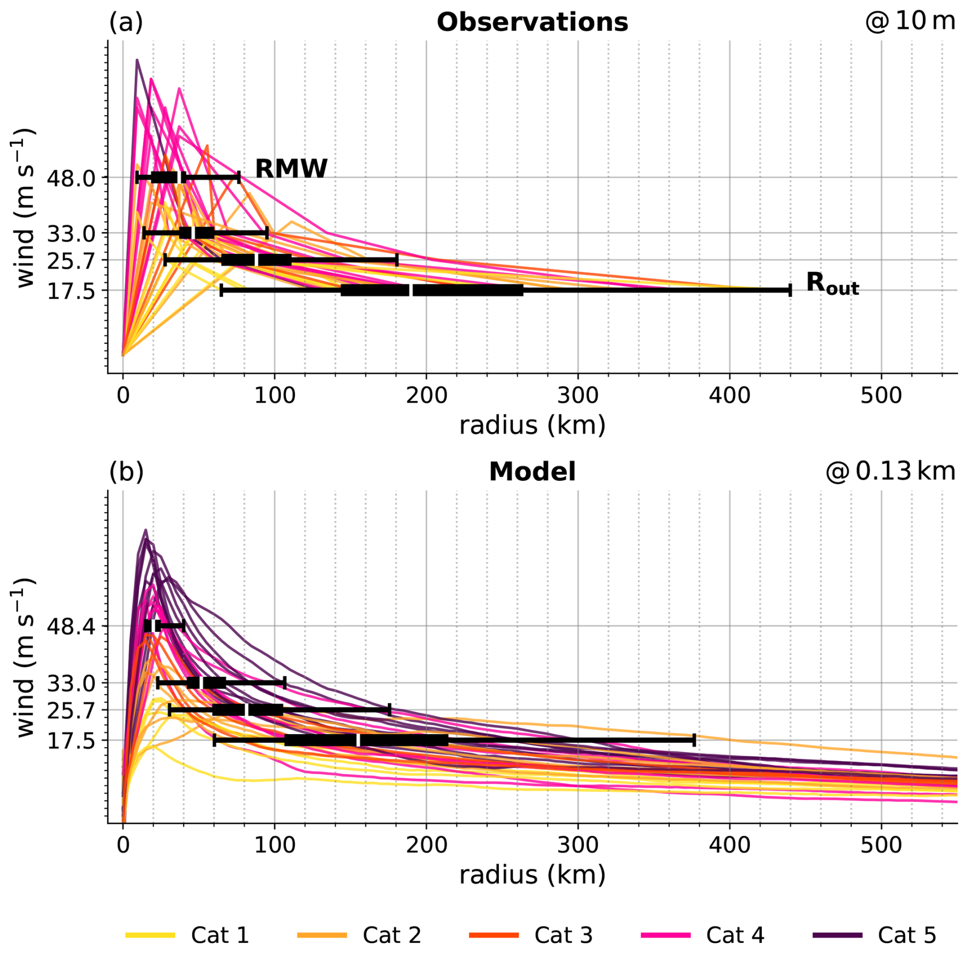
Figure 4 Vortex structures of observed (a) and simulated (b) TCs at maximum intensity (n = 33 for model and observations). Observed wind radii (at 10 m) are taken from HURDAT2 since 2021, where RMW and R_out estimates are available. A zero-velocity point at the center is added for illustration. Simulated winds are azimuthally averaged at 130 m. Box plots show the distribution of commonly used TC wind radii: 17.5 m s⁻¹ (34 knots), 25.7 m s⁻¹ (50 knots), 33 m s⁻¹ (64 knots) and RMW. Lines represent individual TCs, colored by their maximum reached pressure-based category.

4 SyNC case studies

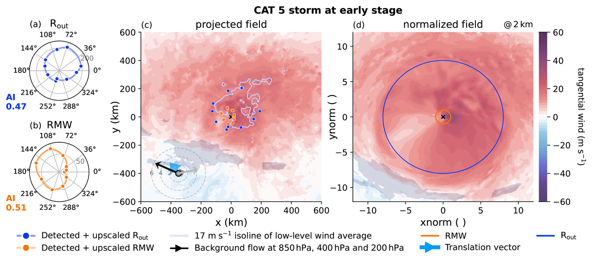
To evaluate the impact of vortex symmetrization and normalization on individual TCs, two case studies are presented in this section. The projected and the normalized tangential wind field of two individual TCs is demonstrated in Figs. 5 and 6. The cat_pres 5 storm (Fig. 5) reveals a typical TC vortex structure, exhibiting a calmer eye, a distinct eyewall and decaying winds at larger distance with an overall asymmetric vortex structure. Before the symmetrization and normalization (Fig. 5c), the tangential wind field is shifted into the northeastern quadrant, likely due to the impact of friction over land and the storm translation vector aligning with the tangential winds. Accordingly, with R_out varying from about 150 km to 600 km, AI of R_out is found to be 0.36 (Fig. 5a). Also RMW shows asymmetry, with an AI of 0.27 (Fig. 5b). After symmetrization and normalization, the vortex becomes symmetric around the storm center (Fig. 5d). RMW and R_out are repositioned to a normalized radius of 1 and 8, respectively. Mesoscale features in the data field are preserved, with only their radial distances adjusted while their angular positions relative to the center remain unchanged.

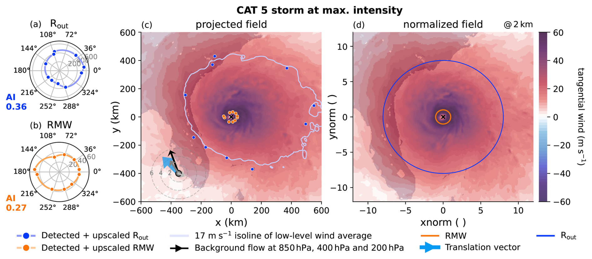
Figure 5 Demonstration of detected wind radii and the effects of SyNC of a cat_pres 5 storm at maximum intensity. Detected (blue points) and upscaled (blue line) R_out (a). Detected (orange points) and upscaled (orange line) RMW (b). The asymmetry index (AI) of R_out and RMW is noted in the left corner of corresponding sub panel. The vortex on the projected grid (c). The cyclone center is marked with a black cross. Contours show the tangential wind field at 2 km height with detected R_out (blue points) and detected RMW (orange points). The light blue line marks the 17 m s⁻¹ contour of the low-level (0–2 km) tangential wind average used for R_out detection. The arrows in the lower-left corner of (c) indicate the background flow at 850 hPa (black), 400 hPa (gray), and 200 hPa (light gray) averaged within 600–800 km horizontal distance of the storm center, as well as the storm's translation vector (blue). Dashed circles provide magnitudes of background winds and translation speeds at levels of 2, 4 and 6 m s⁻¹. The vortex on the normalized grid (d). Contours show the tangential wind field after symmetrization and normalization, where the location of R_out (blue circle) and RMW (orange circle) are highlighted. Dark background shading in (c)–(d) denotes land.

Figure 6 As Fig. 5, but for a cat_pres 1 storm.

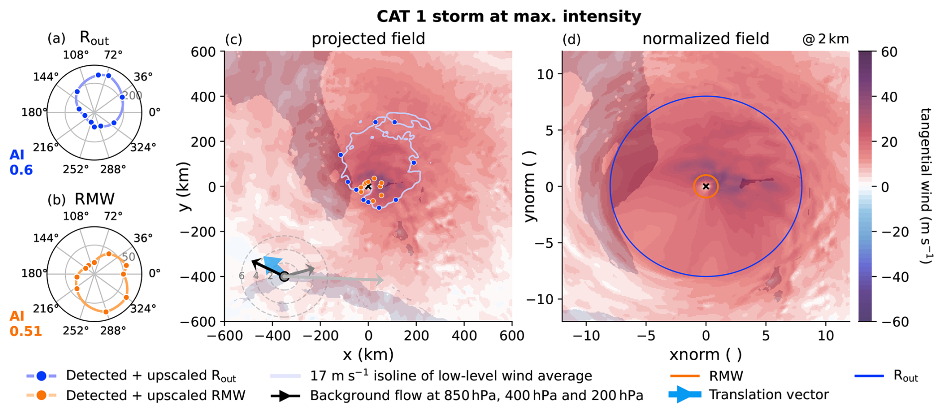
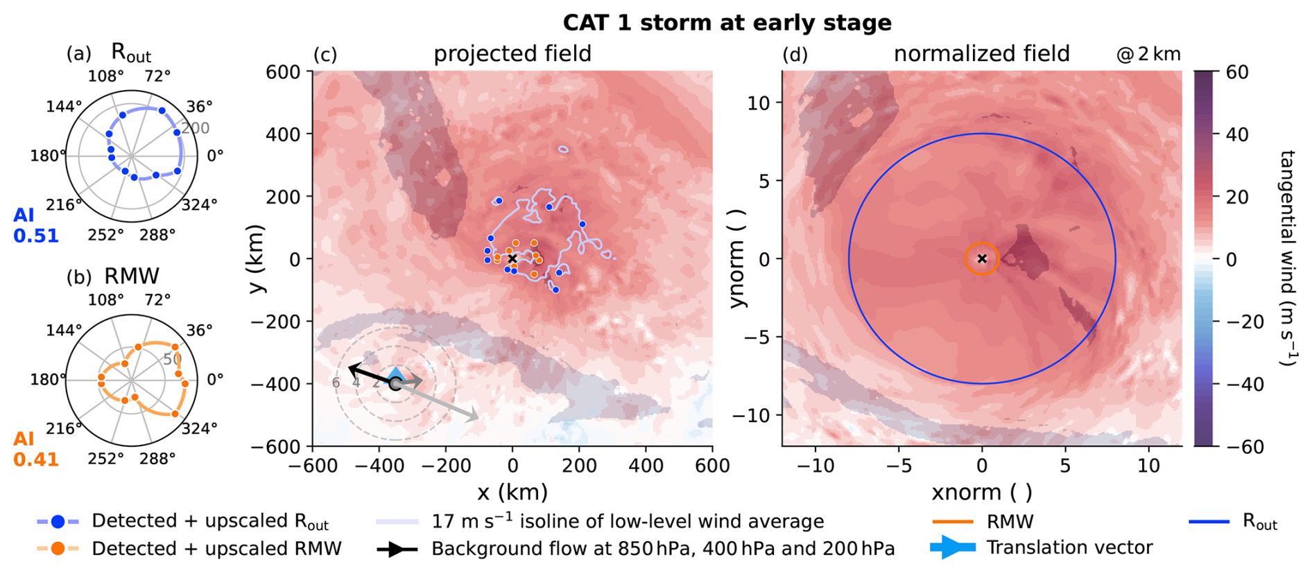
Symmetrization and normalization are more challenging for less well-organized TCs. A cat_pres 1 storm, illustrated in Fig. 6, has not achieved full structural organization, likely due to strong vertical wind shear and interactions with land. The eyewall of this weaker TC is not completely enclosed within the tangential wind field, and the outer wind distribution remains patchy, with several local wind maxima (Fig. 6c). Despite these irregularities, the algorithm was able to approximate both radii. A notable challenge lies in the cat_pres 1 storm's relatively small size and the narrow distance between RMW and R_out in the southwestern quadrant. This resulted in extrapolation of data onto the normalized grid, causing a blurring effect in that quadrant (Fig. 6d). Nevertheless, we consider this drawback to be outweighed by the benefit of achieving symmetry in both the eyewall and the storm boundary. Thanks to the relocation process, even this small storm becomes perfectly aligned with the eyewalls and boundaries of the other TCs in the group during composition.

5 Storm structure evolution

The novel composite method can be used to analyze structure evolution of TCs demonstrated in this section. Fig. 7a–c illustrates the vortex structure evolution of observed (black) and simulated (blue) TCs. The temporal evolution is aligned with respect to the lifetime maximum intensity. Consequently, storm intensities at a given normalized time step may vary. The model and observations show relatively good agreement in the structure evolution throughout the life cycle. Both observed and simulated TCs exhibit a contraction of RMW during the intensification phase reaching minimum RMWs at peak intensity (Fig. 7a), aligning with previous studies (Stern et al., 2015; Qin et al., 2016). The simulated RMW magnitudes generally align well with observations, indicating that the model realistically reproduces eye and eyewall sizes. R_out values slightly increase in the decay phase in both datasets (Fig. 7b). However, simulated R_out values are consistently overestimated due to systematic differences in the detection method, as discussed in Appendix B1. Also, both simulated wind radii are significantly larger than observed values near and shortly after genesis, likely because tangential wind based radii detection is particularly challenging at that stage. Storm size AIs remain relatively constant throughout the life cycle in both observations and simulations (Fig. 7c). This is consistent with the results of Li and Tang (2025), who found that size AI during storm intensification can increase, decrease, or remain constant. Average size AI values are approximately 0.4 for simulated TCs and 0.2 for observed TCs, both with spreads of 0.2. The non-zero AI values confirm that axisymmetry is not present in either dataset, as expected. As discussed in Appendix B2, the higher number of detection sectors in the model likely leads to systematically higher AI values in simulations compared to observations. Both observed and simulated TC groups exhibit substantial within-group variability in vortex structure over the life cycle. In the early stage, the IQR of RMW spans approximately 200 km for simulations and 50 km for observations. In the late stage, model and observations show an IQR of around 100 km. The IQR of R_out remains around 100 km for both datasets throughout the life cycle. These wide spreads in radii and AI highlight the large diversity in vortex structures within both datasets. This underlines the importance of SyNC to precisely align vortex structures for composite analysis.

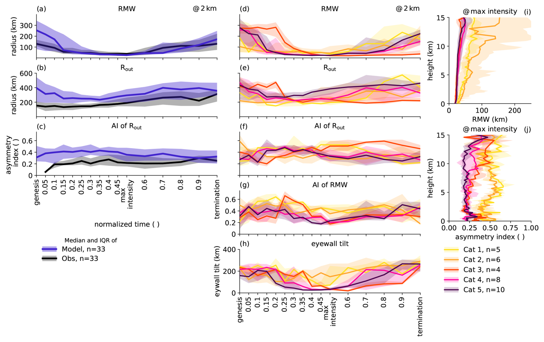
Figure 7 Evolution of TC structure related metrics over the storm's life cycle: RMW (a, d), R_out (b, e), asymmetry index (AI) of R_out (c, f), AI of RMW (g) and eyewall tilt (h). Panels (a)–(c) show a comparison of observed TC structures (HURDAT2 since 2021, black) and simulated TC structures (blue). Simulated TC wind radii and AIs are diagnosed at 2 km altitude, observations correspond to 10 m altitude. Panels (d)–(j) show simulated TCs split according to their lifetime maximum intensity, hence storm intensity can differ within one category before and after reaching maximum intensity. Vertical profiles of RMW (i) and RMW AI (j) are displayed at maximum intensity. The eyewall tilt is estimated as the difference between the minimum and maximum of the vertical profile of RMW between 0–15 km. Lines display the group's median and the shaded area represents the interquartile ranges (IQRs). Normalized time ticks indicate the frequency of diagnosed radii and AIs setting a focus on the intensification phase.

Since Li and Tang (2025) found that weaker TCs typically exhibit larger size asymmetries, often as a consequence of stronger VWS, we analyze the vortex structure evolution for storms separately according to their maximum pressure category, as illustrated in Fig. 7d–i for simulated TCs. The storm size and size asymmetry are both not significantly changing between the various storm intensities in the model (Fig 7e, f), contradicting results of Li and Tang (2025). On the contrary, the eyewall evolution shows distinguishable differences between weak and strong TCs (Fig. 7d). While all storm categories indicate the RMW contraction, it is much more pronounced for cat_pres 4 and 5 TCs, which produce the smallest eyewall radii at maximum intensity. This is also visible throughout all vertical levels (Fig. 7j).

The eyewall asymmetry also displays some change over the life cycle especially for cat_pres 3–5 TCs. At an early stage of the life cycle, RMW AIs start at relatively high values around 0.5 for all TC categories (Fig. 7g). The asymmetry of the eyewall remains at high levels also for weak TCs. However, intense TCs reveal a symmetrization of their RMW during the second half of their intensification phase, when AI drops approximately from 0.4 to 0.2. This is in agreement with previous studies (Persing et al., 2013; Martinez et al., 2022), which found that eyewall symmetrization and associated convective organization is beneficial for TC intensification. Cat_pres 3–5 TCs also exhibit a reduction in eyewall tilt during intensification and significantly smaller eyewall tilt than weaker TCs at maximum intensity (Fig. 7h, i). These results are consistent with previous observational and modeling studies that found smaller eyewall tilts in more intense TCs (Shea and Gray, 1973; Sanabia et al., 2014; Ohno et al., 2016).

6 Composite sharpening by SyNC

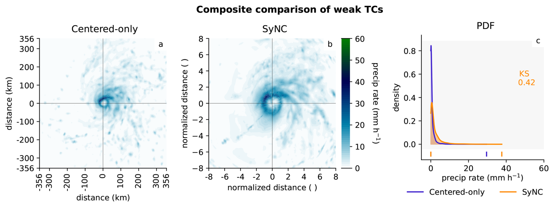
To assess the performance of SyNC and identify its benefits and limitations, SyNC composites are compared with composites in which only the storm centers are aligned (centered-only). The underlying TC groups are identical for both composite methods. For compositing, simulated TCs were split into weak (cat_pres 1–3, n = 15) and intense (cat_pres 4–5, n = 18) TC groups allowing to detect systematic differences in the SyNC performance between differently intense TCs. Moreover, these groupings maximize structural variability within the weak TC group and minimize it within the intense group based on the results shown in Fig. 7. This design enables an assessment of which TC group benefits most from the SyNC approach, the structural more homogeneous (intense) or more inhomogeneous (weak) group.

6.1 Preserved mesoscale features

This section evaluates the ability of SyNC to preserve mesoscale features in composites. Data fields are identified, which do or do not benefit from SyNC, thereby clarifying its relevance for different research applications. A comparison of the two composite methods of the intense group composed at their lifetime maximum intensity can be found in Figs. 8 and 9 (and additional data fields in Fig. D1 in Appendix D). Overall, the SyNC composite fields often reveal more pronounced extreme values in the vertical cross sections (positive and negative) compared to the centered-only composites, as illustrated by the probability distribution functions (PDFs) of respective fields (Fig. 8c, f, i and l). The enhanced extremes are attributed to improved alignment of vortex structures and associated storm features, which helps preserve these characteristics more effectively in the group average. Most fields show substantial improvement due to the SyNC method's alignment of the eyewall: Vertical winds indicate stronger eyewall updrafts and stronger downdrafts within the eye (Fig. 8b). Temperature tendencies of the cloud microphysical scheme reveal approximately 10 K h⁻¹ higher latent heating within the eyewall (Fig. 8e). Additionally, stronger cooling (evaporative cooling of rain and ice melting), is more distinctly positioned on the inner and outer flanks of the eyewall updraft. Cloud water and precipitation (Fig. D1e and h) also show extended maxima within the eyewall. Surface precipitation rates (Fig. 9) are also better preserved by SyNC indicating maximum rates 10 mm h⁻¹ higher than in the centered-only approach. This highlights the improved representation of microphysical signals and precipitation achieved by vertically aligning the eyewalls throughout the depth of the TCs, with implications for physical understanding and TC risk assessments. The super-gradient outflow above the boundary layer (Fig. 8h) is sharpened in the SyNC composite. Tangential winds not only show a larger peak near the eyewall in the lower atmosphere (Fig. 8k), but also indicate stronger winds throughout the vortex due to a better alignment of the vortex borders. The border alignment avoids overlaying environmental and storm regions, which also benefits the equivalent potential temperature field (Fig. D1k). The SyNC composite maintains a higher θ_e especially in the storm's outer region. However, due to the relatively uniform radial nature of the θ_e field, it gains the least from the SyNC compositing. A similar behavior is found for water vapor and longwave radiative cooling, both of which are also radially uniform (Fig. D1n and q).

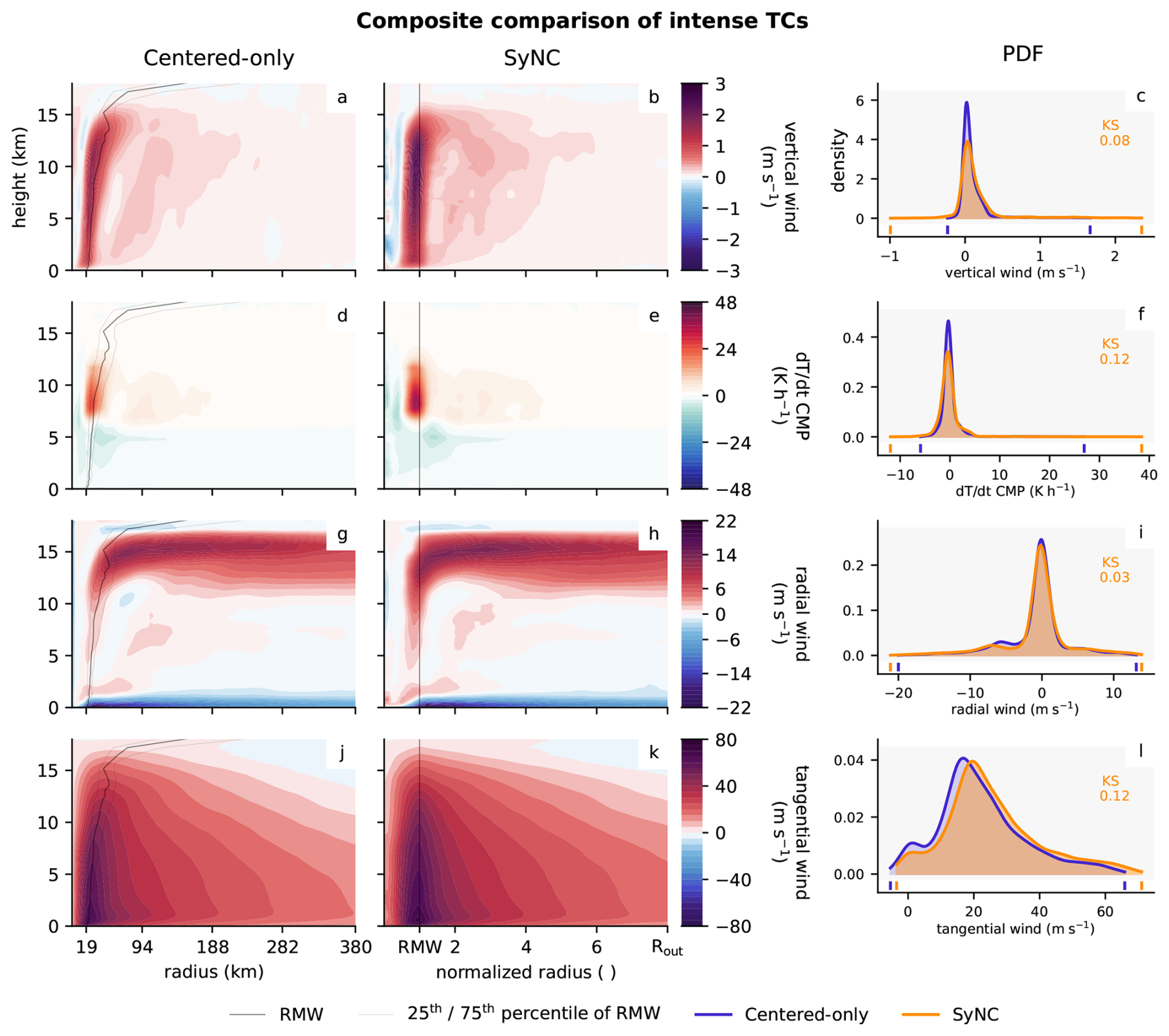
Figure 8 Comparison of centered-only (a, d, g, j) and SyNC composites (b, e, h, k) of the intense TC group (n = 18) at lifetime maximum intensity, showing the azimuthally averaged cross sections of vertical wind (a, b), temperature tendencies from the cloud microphysical scheme ($\mathrm{d}T/\mathrm{d}t$ CMP, d, e), radial winds (g, h) and tangential wind (j, k). The extent of the cross sections is set to the average R_out detected over the TC group. RMW is indicated with a black line, whereof the spread of the eyewall location is shown by the two gray lines for the centered-only approach. Panels (c), (f), (i) and (l) show the probability distribution functions (PDFs) of the cross section data fields of the centered-only (blue) and the SyNC (orange) composite methods. Minima and maxima of the PDFs are illustrated by blue/orange ticks on the x-axis. The Kolmogorov-Smirnov (KS) test statistic between the two distributions is noted in each sub panel.

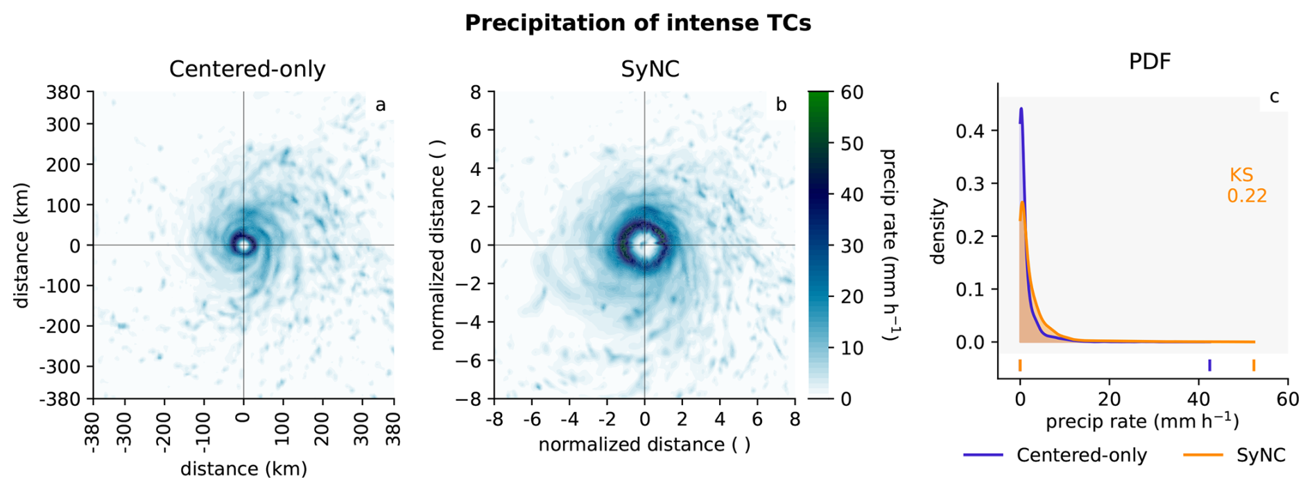
Figure 9 Plan view of surface precipitation rates for centered-only (a) and SyNC composites (b) of the intense TC group (n = 18) at lifetime maximum intensity. The extent of the plan view is set to the average R_out detected over the TC group. Panel (c) shows the probability distribution function (PDF) of the data fields of the centered-only (blue) and the SyNC (orange) composite methods. Minima and maxima of the PDF are illustrated by blue/orange ticks on the x-axis. The Kolmogorov-Smirnov (KS) test statistic between the two distributions is noted in the sub panel.

Similar results are found for the weak storms (Figs. D2, D3 and D4), which are structurally more variable than the intense one. It is worth mentioning that due to the large variability of eyewall radii in the weak group, secondary peaks in updraft (Fig. D2a) or latent heating (Fig. 11a) may be misinterpreted as features of outer rainbands. However, the SyNC composite clarifies that these are indeed eyewall features.

To statistically quantify the impact of the SyNC compositing method, the Kolmogorov-Smirnov (KS) test statistic is calculated for each variable, measuring the distance between the PDFs of the centered-only and SyNC composite fields. Overall, KS statistics of the weak group (Figs. D2c, f, i and l, and D4c) are comparable to or higher than those of the intense group (Figs. 8c, f, i and l, and 9c), suggesting that the weak group benefits slightly more from the SyNC approach. Accordingly, the benefit of preserving mesoscale features by SyNC depends on the degree of structural variability within the TC group, with the benefit likely emerging even for a relatively small TC group size. Nevertheless, with overall KS statistics of around 0.1 and larger extreme values, the SyNC method successfully sharpens the composite fields of both, weak (i.e., structurally varying) and intense (i.e., structurally more uniform) cyclone groups.

6.2 Enhanced statistical power

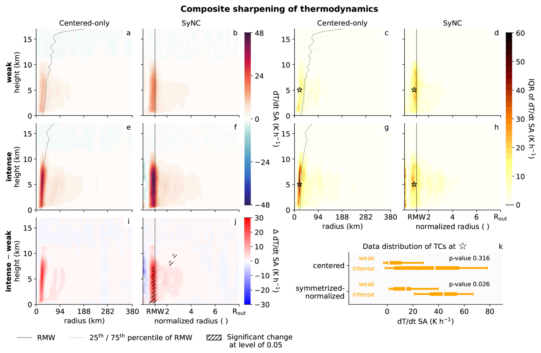
In addition to preserving mesoscale features, SyNC is found to enhance the sensitivity of statistical tests between cyclone groups as demonstated in this section. Figures 10 and 11 display the radial wind and temperature tendencies due to saturation adjustment (parametrized cloud droplet growth) for both the weak and intense TC group, along with their differences. Statistically significant differences between the two groups are determined via a false-discovery rate corrected permutation test at a 0.05 significance level and are indicated by the hatched areas (Figs. 10i, j and 11i, j). Interestingly, the regions of significant change differ between the two compositing methods, although the underlying cyclone groups are identical. While the centered-only composite shows the most prominent differences in radial winds, it misses several mesoscale features that are detected by the SyNC composite (Fig. 10j): Significantly stronger super-gradient outflow above the boundary layer, significantly stronger inflow throughout the vortex and significantly stronger mid-level outflow, potentially induced by rainbands, for intense TCs. There are two main reasons for these differences in detected significance. First, the SyNC composite better aligns the vortex and their mesoscale features, which can amplify the observed differences between the two groups, as shown in Figs. 10j and 11j. Second, the eyewall alignment can reduce the data spread within a TC group, thereby improving the statistical power of the statistical test (Krzywinski and Altman, 2014). The within-group spread of radial wind is illustrated by the IQR cross sections of each TC group per composite method in Fig. 10c, d, g, h and k. Radial wind IQRs of weak TCs are relatively similar between the composite methods. On the contrary, the intense TCs exhibit a large IQR in the centered-only composite around the eyewall, which is nearly twice that of the intense SyNC composite. To illustrate the impact of the large IQR on the power of the statistical test, box plots (Fig. 10k) show the radial wind distributions of all TCs at a selected grid cell (black star) for both composite methods. For the radial wind, the selected grid cell is located at low levels at the inner side of the eyewall, where super-gradient outflow is forming. First, the box plot medians of two cyclone groups are slightly more apart in the SyNC composite than in the centered-only composite. Second, the IQR of the centered-only intense TCs is larger than for the SyNC composite, spreading from negative (inward) to positive (outward) radial winds. This large IQR likely is a result of the their distinct though slightly displaced eyewalls: At the selected grid cell, inflow is observed for TCs with more narrow eyewalls, while for others already super gradient wind is formed at this distance. The resulting large within-group spread in the data causes the storm group distributions to overlap much more for the centered-only composite than for the SyNC composite, which increases the p-value of statistical testing for the centered-only composite. The eyewall alignment of the SyNC composite results in only outward radial winds at selected grid cells narrowing the within-group spread and reducing the p-value allowing for the detection of a significant difference between the TC groups with the SyNC approach. In the temperature tendency due to saturation adjustment (Fig. 11), the centered-only composite method even fails to detect any significant changes (Fig. 11i), whereas the SyNC method reveals significantly enhanced latent heating in the intense storms (Fig. 11j), as expected. Controversy, the median differences between the weak and intense TCs is slightly larger for the centered-only approach (Fig. 11i, k) than for SyNC. In the SyNC approach, especially the weak group benefits from the eyewall alignment resulting in the amplification of the heating signal (Fig. 11b) there producing smaller median differences between the weak and intense TC groups (Fig. 11k). However, the within-group variance reduction of the intense TCs by the SyNC composite (Fig. 11h, k) increases the sensitivity of the statistical testing, outweighing the smaller median differences, and hence detecting a significant difference between the two groups (Fig. 11j). Thus, by mitigating small eyewall displacements and reducing within-group variance, the SyNC composite proves valuable even for relatively well-organized, more homogeneously structured TC groups, increasing the accuracy of statistical analyses.

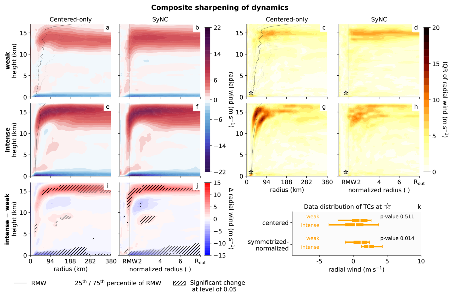
Figure 10 Composite sharpening of radial winds and its influence on statistic testing between weak and intense TC groups at lifetime maximum intensity: The centered-only composite (a, e, i) of weak TCs (n = 15, a), intense TCs (n = 18, e) and their difference (i). Panels (b), (f) and (j) show the same, but for the SyNC composite. Hatched areas (i, j) indicate statistically significant differences between the two TC groups based on a false-discovery rate corrected permutation test at a 0.05 significance level. The interquartile ranges (IQRs) of each grid cell of both composite methods are shown in (c), (d), (g) and (h): centered-only weak (c), centered-only intense (g), SyNC weak (d) and SyNC intense TCs (h). The black star highlights one selected grid cell, at which location the data distribution of the TC groups is displayed in (k). The p-value at the selected grid cell is indicated within the subpanel (k). For the centered-only cross sections, the extent of the cross sections is set to the average R_out detected over the intense TC group, since the mean R_out of the weak TC group is smaller. RMW is indicated with a black line, whereof the spread of the eyewall location is shown by the two gray lines.

Figure 11 As Fig. 10, but for temperature tendencies due to saturation adjustment ($\mathrm{d}T/\mathrm{d}t$ SA).

7 Conclusions

We presented the SyNC composite approach, that accounts for TC size, eyewall location and asymmetry, aiming to preserve mesoscale features in composite fields. The symmetrization and normalization process involves sector-wise detection of RMW and R_out (R17), followed by a sector-wise radius transformation to a normalized radius and data interpolation onto the normalized grid.

SyNC compositing is applied to TCs simulated by ICON at a convection-permitting horizontal grid length of 5 km. While ICON produces fewer storms per season than observed, it is capable of generating the most intense storms. However, ICON tends to overestimate the frequency of major hurricanes while underestimating the frequency of weaker storms. These model biases may be attributable to limitations of the chosen model configuration, such as the absence of atmosphere-ocean coupling.

The sector-wise detection of RMW and R_out enabled by the SyNC approach allows for precise analysis of TC structures. The structural evolution of the simulated TCs reveals eyewall contraction, eyewall symmetrization and eyewall tilt reduction during intensification, particularly pronounced in intense storms, aligning well with findings from previous studies (Stern et al., 2015; Qin et al., 2016; Martinez et al., 2022; Persing et al., 2013; Ohno et al., 2016; Shea and Gray, 1973; Sanabia et al., 2014). Additionally, the structural evolution highlights substantial structural variability and pronounced axis-asymmetries across all storm intensities in both simulated and observed TCs, underscoring the importance of SyNC composites in TC analysis. By aligning the eyewall and vortex boundaries during SyNC compositing, the resulting composite fields are sharpened, as evidenced by higher extreme values in the SyNC composite. This method more accurately captures mesoscale features such as super-gradient outflow above the boundary layer, eyewall updrafts, and subsidence within the eye as well as cloud properties and associated latent heating and cooling. It also more accurately represents regions at the vortex border improving estimates of tangential winds, outer boundary layer inflows and storm's moist entropy, since less environmental air is averaged into the composite field. Furthermore, it reduces within-group variance. While preserving mesoscale features is particularly beneficial for storm groups with diverse shapes, within-group variance reduction is especially advantageous for more uniformly shaped but intense storms, where small displacements of strong signals can significantly increase the group's IQR. Together, preserving mesoscale features and reducing within-group variance enhance the power of statistical testing, enabling the detection of differences between storm groups, that would be missed using a centered-only composite approach.

SyNC is particularly well suited for feature-to-feature comparisons and it enables the identification of variability among individual features. If the focus is instead on field magnitudes or variability at a fixed distance from the storm center, SyNC is less suitable, as the true radial distance from the TC center is no longer preserved and the identified variability by SyNC does not correspond to the variability at a given radius. Moreover, the SyNC compositing method is less effective for radially uniform fields, such as water vapor or longwave radiative temperature tendencies. It is also less suitable during the early stages of a storm’s life cycle, when the vortex is not yet fully developed in the tangential wind field. Moreover, a challenge for the eyewall detection arises from secondary eyewalls since within the current implication, only one eyewall can be defined. Secondary eyewalls are only identified as the primary eyewall once they exceed the primary eyewall in tangential wind strength within a given detection sector. This limitation also suggests a potential use of SyNC for investigating the formation of secondary eyewalls. The transition point at which the secondary eyewall becomes dominant may induce a sudden increase in the RMW within individual sectors and may temporarily increase eyewall asymmetry. Accordingly, variations in RMW and/or eyewall AI could be used to identify secondary eyewalls or even eyewall replacement cycles, a hypothesis that could be tested in future work. A further limitation of SyNC is the need for data interpolation onto the normalized grid, which may lead to extensive extrapolation in small TCs or when RMW and R_out are close together. Therefore, a careful definition of the normalized grid is essential.

Based on the performance of SyNC evaluated in Sect. 6, we identify potential for its application to both observational and simulated TC datasets that resolve mesoscale features and TC structural variability, based on previous studies likely requiring a horizontal grid length of ≈ 10–20 km or finer (Sena et al., 2024; Zhang et al., 2021; Manganello et al., 2012; Judt et al., 2021; Chen et al., 2007). For satellite data, or when tangential wind is unavailable, the TC symmetrization and normalization approach could be adapted to alternative data fields, provided they are strongly linked to eyewall structure and storm size. In such cases, suitable thresholds (e.g., for defining the vortex border) would need to be determined. Improvements to the SyNC method could include refining detection strategies during the early life cycle stages and at upper levels, where anticyclonic outflow complicates currently implemented radius detection. A different detection method of the vortex center and a vertically varying vortex center could further improve the precision of composites. For wind shear studies, rotating the field according to the shear vector may offer further enhancements. Despite these limitations, the SyNC compositing method significantly improves the accuracy of TC composites and enables reliability of statistical testing of the overall storm structures and mesoscale features by overcoming the challenges of various vortex structures. Although the normalization results in the loss of true spatial distances within the vortex, it offers a cyclone-relative framework that facilitates distinguishing between processes occurring within the eyewall and those in the outer regions of the TC. The sector-wise detection of RMW and R_out enables high-precision analysis of vortex asymmetries, storm size, and eyewall structures. As such, the SyNC composite method is well-suited for a wide range of research applications.

Appendix A: Simulated and observed TC tracks

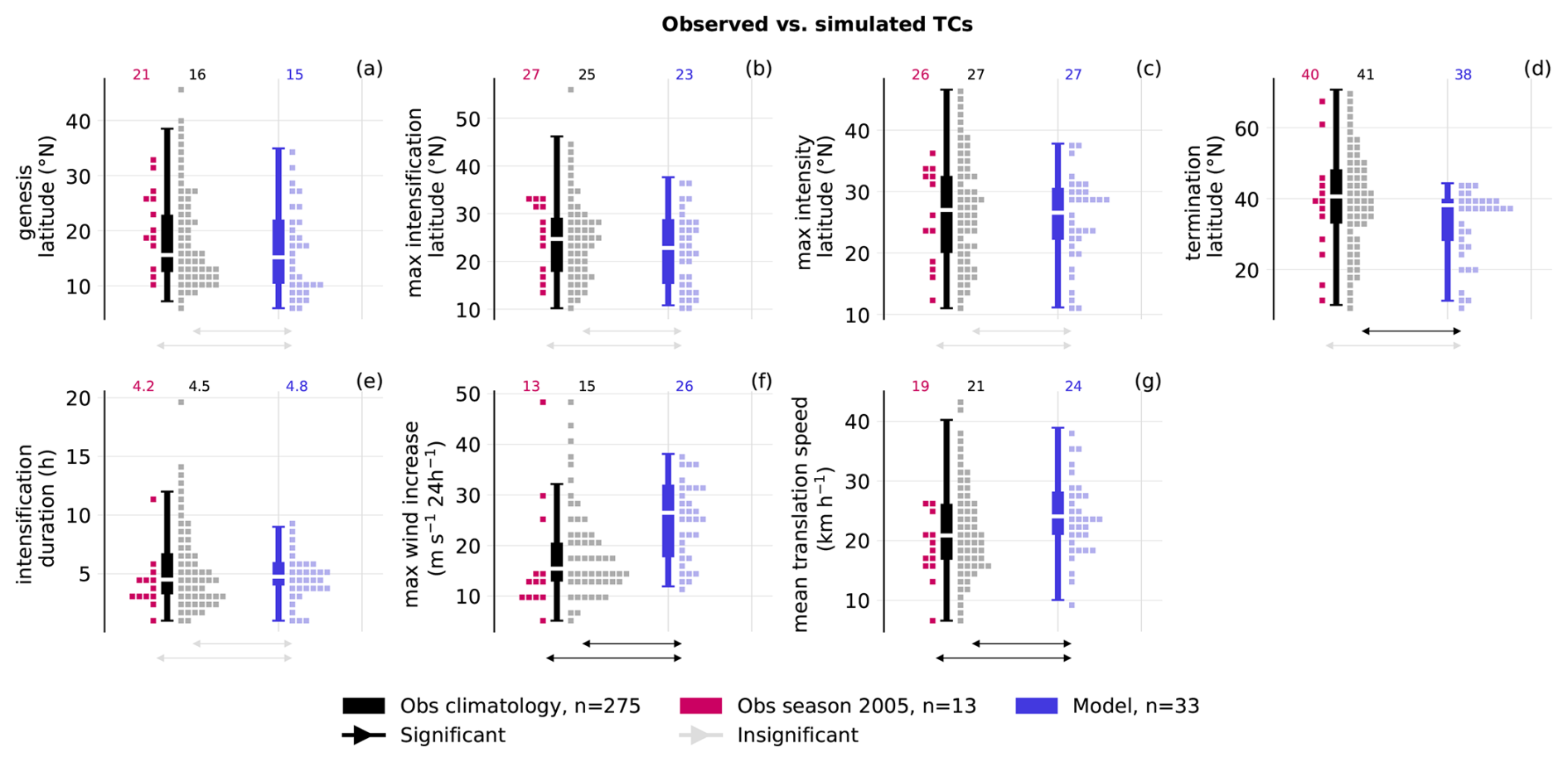
To validate the simulated TCs, tracks from the eight ensemble members are compared with observed tracks from the HURDAT2 dataset (Landsea and Franklin, 2013) (Figs. A1 and A2). Overall, the eight ensemble members (Fig. A1a) partially reproduce the observed TC tracks (Fig. A1c). The simulations capture genesis events south of the domain between 5–15° N but fail to reproduce some genesis farther north-east of the domain over cooler sea surface temperatures. Despite this, there is a good latitudinal agreement between simulated and observed locations of genesis, maximum intensity, and termination evident in Fig. A2a–d, although it is strongly influenced by the model domain. A comparison using a single ensemble member (Fig. A1b) further illustrates that the total number of simulated TCs is underestimated. In addition, the simulated tracks do not precisely match the observed trajectories because the model is only forced by the 2005 large-scale environment at the lateral boundaries and no nudging within the domain was applied. Perturbed initial conditions among the ensemble members further contribute to a model spread. Consequently, the simulated TC tracks diverge from observations.

Comparison of translation speed (Fig. A2g) shows that simulated TCs propagate faster than observed TCs. Simulated storms also intensify more rapidly (Fig. A2f), while the duration of the intensification phase (Fig. A2e) is approximately comparable to observations. This is consistent with the tendency for simulated TCs to be more intense on average than observed TCs.

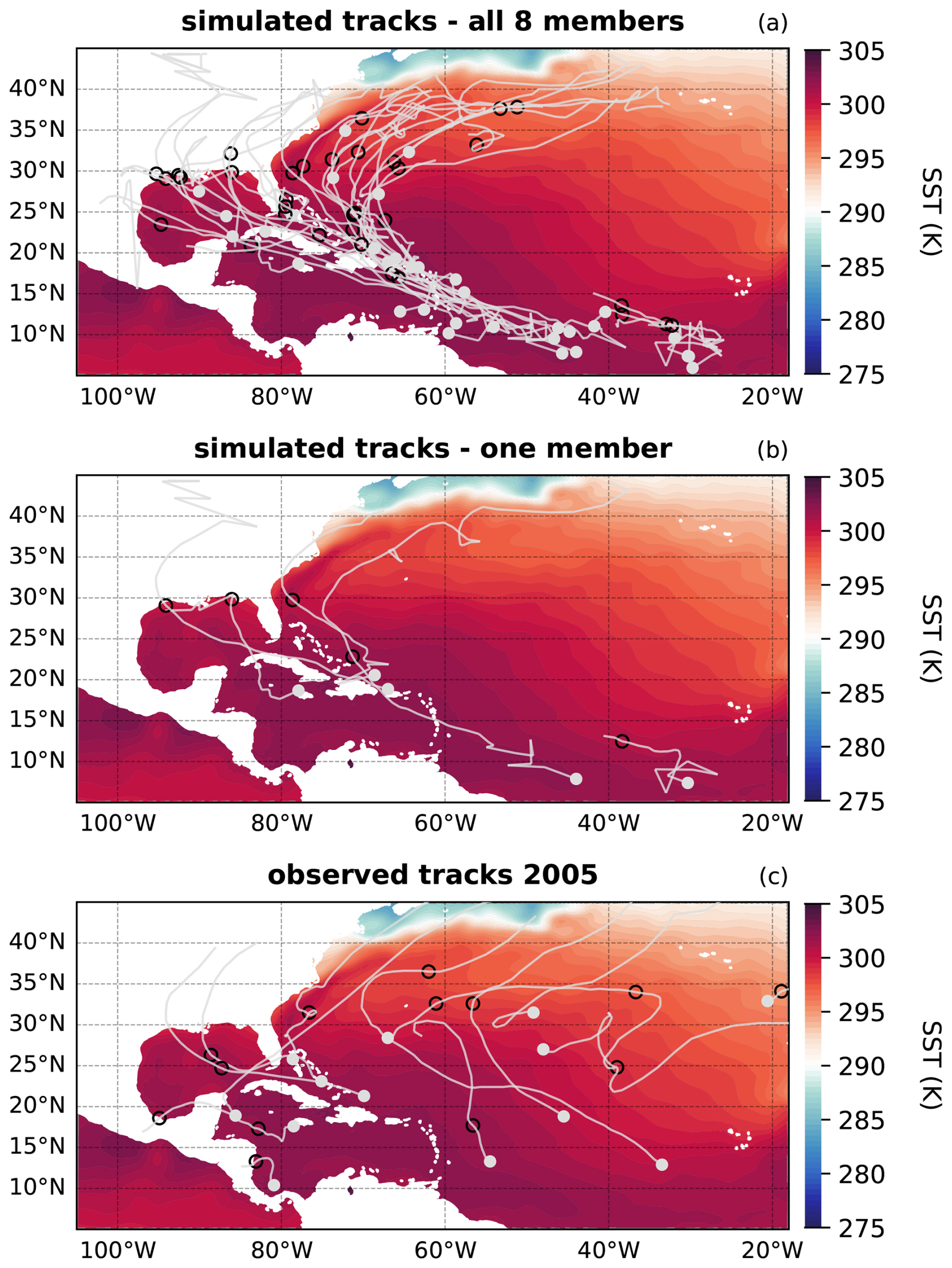
Figure A1 TC tracks of all eight simulated members (a), one simulated member (b) and observations in 2005 (HURDAT2, filtered for July to December c) in the North Atlantic. Filled gray circles denote TC genesis locations, and black circles mark the position of maximum intensity. Shading indicates the model sea surface temperature (SST) boundary conditions, averaged from July to December 2005 (from the ECMWF IFS HRES analysis).

Figure A2 As Fig. 3, but for genesis latitude (a), latitude of maximum intensification (b), latitude where maximum intensity is reached (c), termination latitude (d), intensification duration (e), wind increase over 24 h (f) and mean translation speed (g).

Appendix B: SyNC configurations

B1 R_out detection layer

The symmetrization and normalization of TCs require a selection of several parameters to avoid unphysical radius detection and to ensure algorithm robustness, especially for atypical storm structures that may occur during the early or late stages of a storm's life cycle or in weak systems. To enhance robustness and better represent storm size, R_out is not detected on tangential winds at a single vertical level, but rather on the averaged vertical wind over a thicker layer. This detection layer extends from the lowest model level (approximately 60 m) up to a selected altitude. Various detection layer thicknesses were tested ranging from 130 m to 6 km (Fig. B1, brown to blue box plots) to assess the sensitivity of R_out to the choice of the detection layer. Observed R_out are included as reference (black). All tested detection layers yield larger R_out values than observed ones. However, the model successfully reproduces the spread of observed R_out's at all life cycle stages. For all life cycle stages, R_out increases with detection layer thickness up to 2 km, then decreases for thicker layers. This behavior can be attributed to the tangential winds, which typically peak around 2 km altitude. The sensitivity is smallest at the early stage. At maximum intensity and in the late stage, R_out can vary by approximately 70 km. Since R_out defines the vortex boundary in the SyNC composite, we select the detection layer that yields the largest possible vortex boundary being the layer up to 2 km. This conservative approach maximizes the inclusion of data points, while acknowledging that it introduces a systematic bias when comparing R_out to observations.

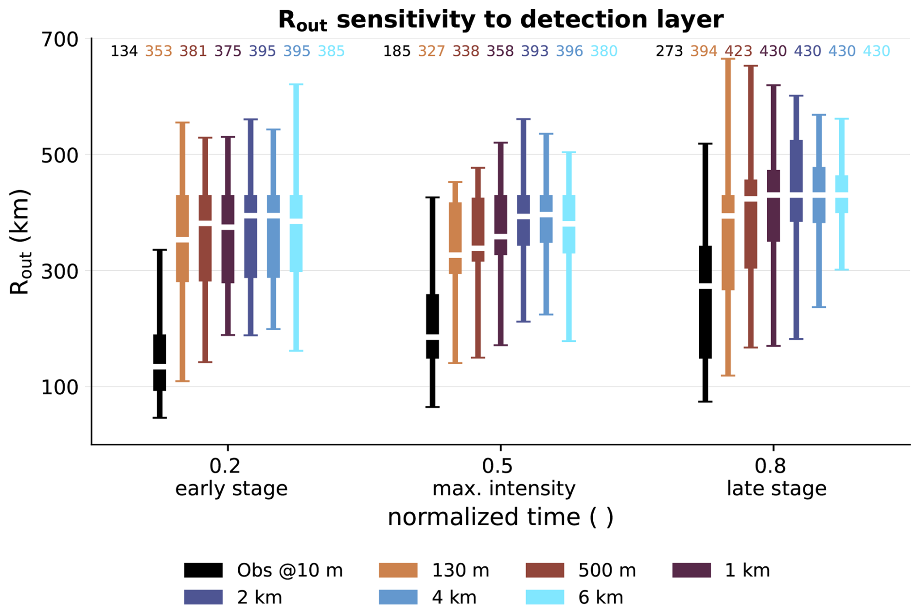
Figure B1 Sensitivity of R_out to the detection layer thickness: The colored box plots show the distribution of the detected R_out (median over the 10 detection sectors) for all the simulated TCs (n = 33) based on the detection layers reaching from 130 m to 6 km (brown to blue). The black box plots show the distribution of observed R_out at 10 m (median over the 4 observation sectors). The sensitivity analysis is performed at three TC life cycle stages: early stage, maximum intensity, and late stage. Box plots medians are indicated above each box plot.

B2 Number of detection sectors

To assess potential benefit of using a large number of detection sectors, we calculated AIs for RMW and R_out, based on radii detected in 4, 6, 8, or 10 sectors (Fig. B2, brown to blue). The AI of R_out and its spread increase with the number of detection sectors, suggesting that more sectors capture the vortex border asymmetry more accurately. Using only 4 sectors may underestimate AI by about 0.2 to 0.3 throughout the life cycle. Notably, AI of R_out is not saturated even with 10 sectors, especially in early stages. Although the 5 km horizontal grid length limits us to a maximum of 10 sectors (Sect. 2.6), using more sectors could further improve AI estimates. Observed AI of R_out (black), based on 4 sectors, is slightly higher than the simulated 4-sector AIs of R_out. The 6-sector AI of R_out aligns well with observations, while 8- and 10-sector AIs exceed them. For RMW, no sector-wise observations are available. Still, simulated AIs of RMW show similar trends: higher AI and greater spread with more sectors at peak intensity. The AI gain from 4 to 10 sectors is about 0.1. Accordingly, RMW AI benefits slightly less from more detection sectors than AIs of R_out. At early and late stages, AI appears to saturate between 8 and 10 sectors. Overall, using 10 detection sectors performs best for both radii AI estimates, so we proceed with 10 sectors in this paper.

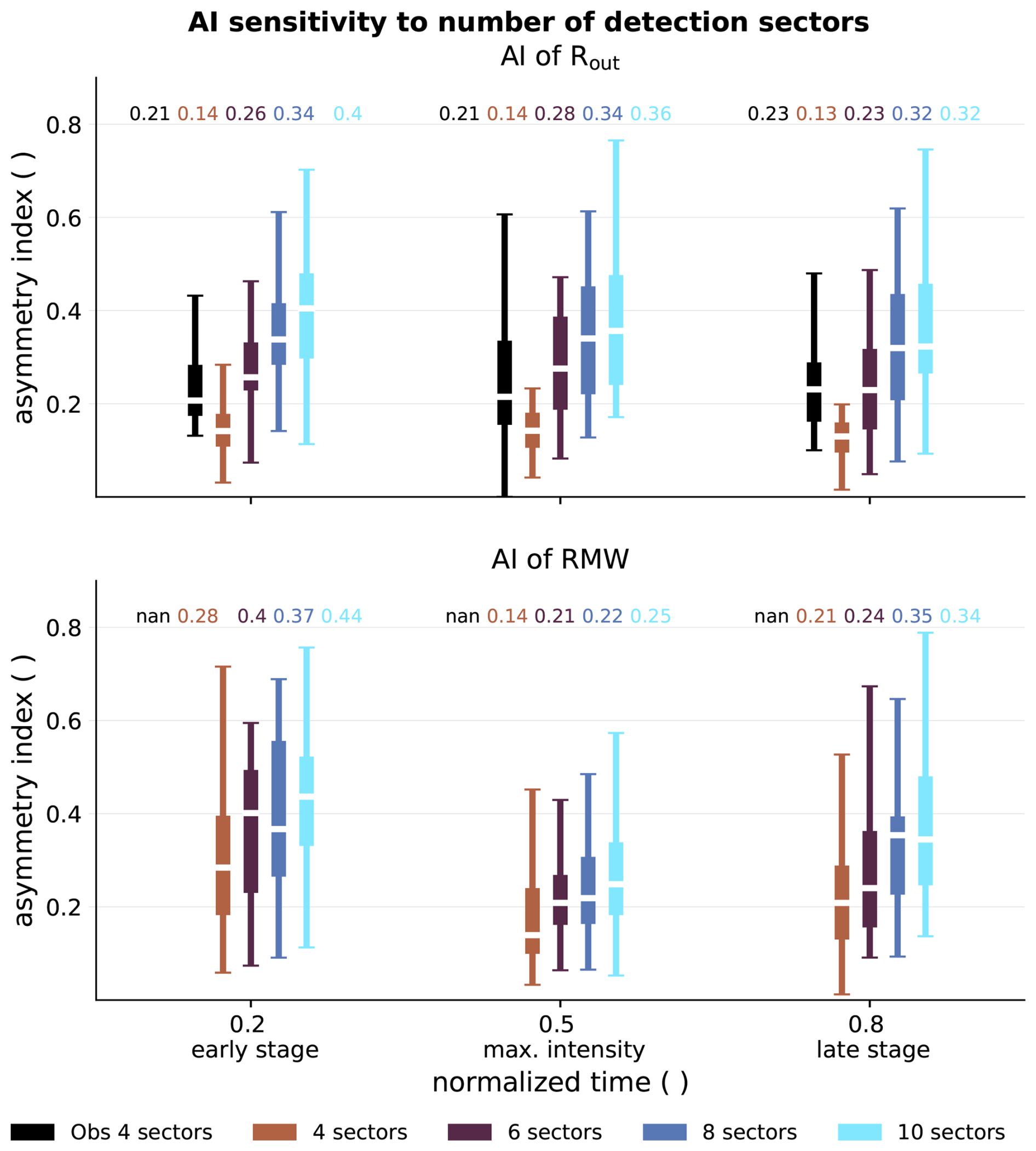
Figure B2 Sensitivity of the asymmetry index (AI) to the number of detection sectors: Colored box plots show the distribution of AIs for all the simulated TCs, where AI is detected based on 4, 6, 8 or 10 detection sectors (brown to blue). The top panel shows AIs of R_out, the bottom panel AIs of RMW. The black box plot indicates observed AI of R_out based on 4 sectors. No observed RMW AI are available. The sensitivity analysis is performed at three TC life cycle stages: early stage, maximum intensity, and late stage. Box plot medians are indicated above each box plot.

B3 Thresholds

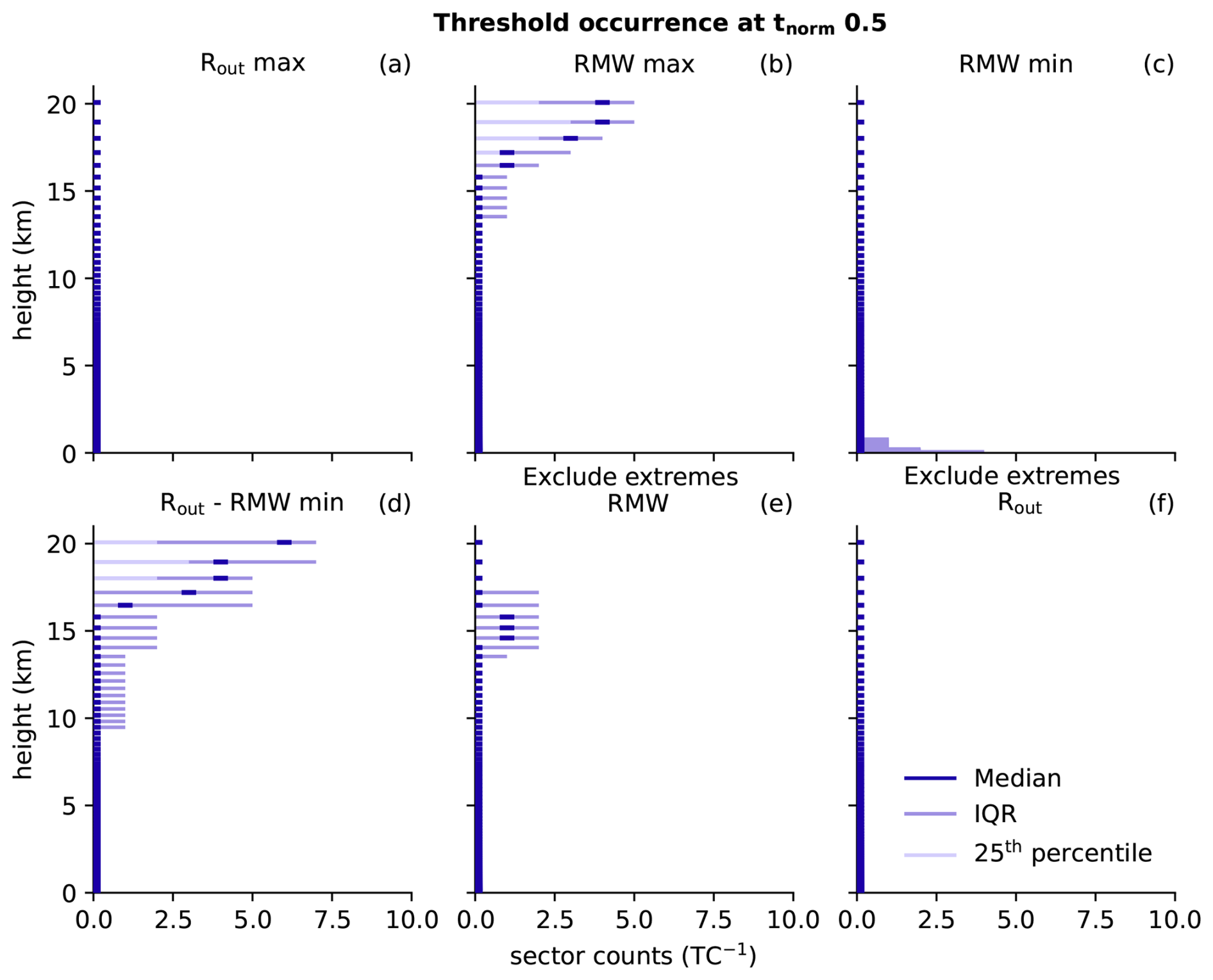
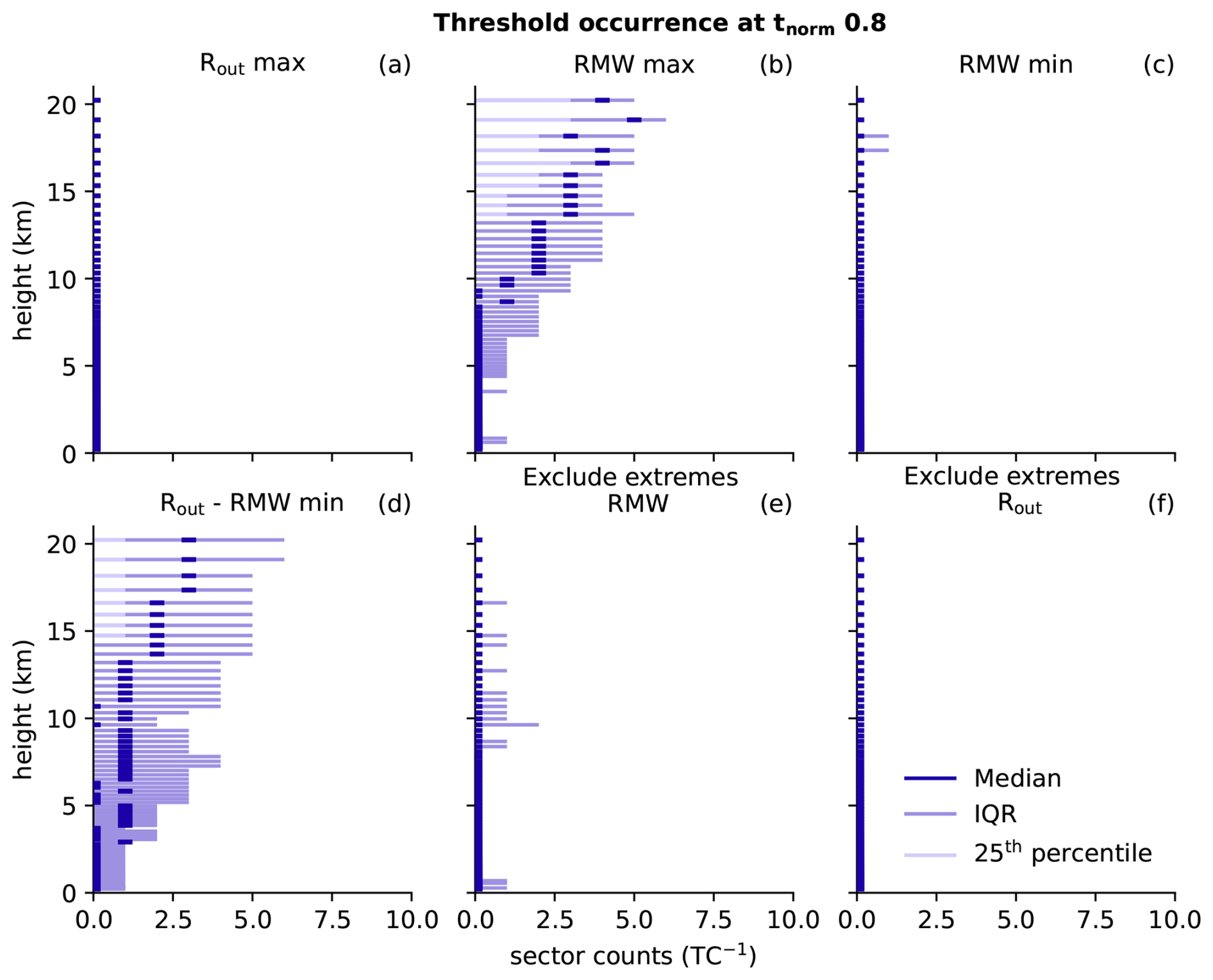
To make the radii detection robust, some thresholds regarding RMW and R_out are implemented. Figure B3a shows the observed values for RMW, R_out and their difference, which guided the selected minimum thresholds. Figure B3b illustrates the limitation of the data resolution on the selection of number of detection sectors.

Figures B4, B5 and B6 show where and when the six thresholds where applied during detection. The most applied threshold is maximum RMW and minimum distance between RMW and R_out. Thresholds where most frequently applied at upper-levels where the tangential wind turned into an anticyclonic rotation and at early and late stages, where the vortex structure is less organized.

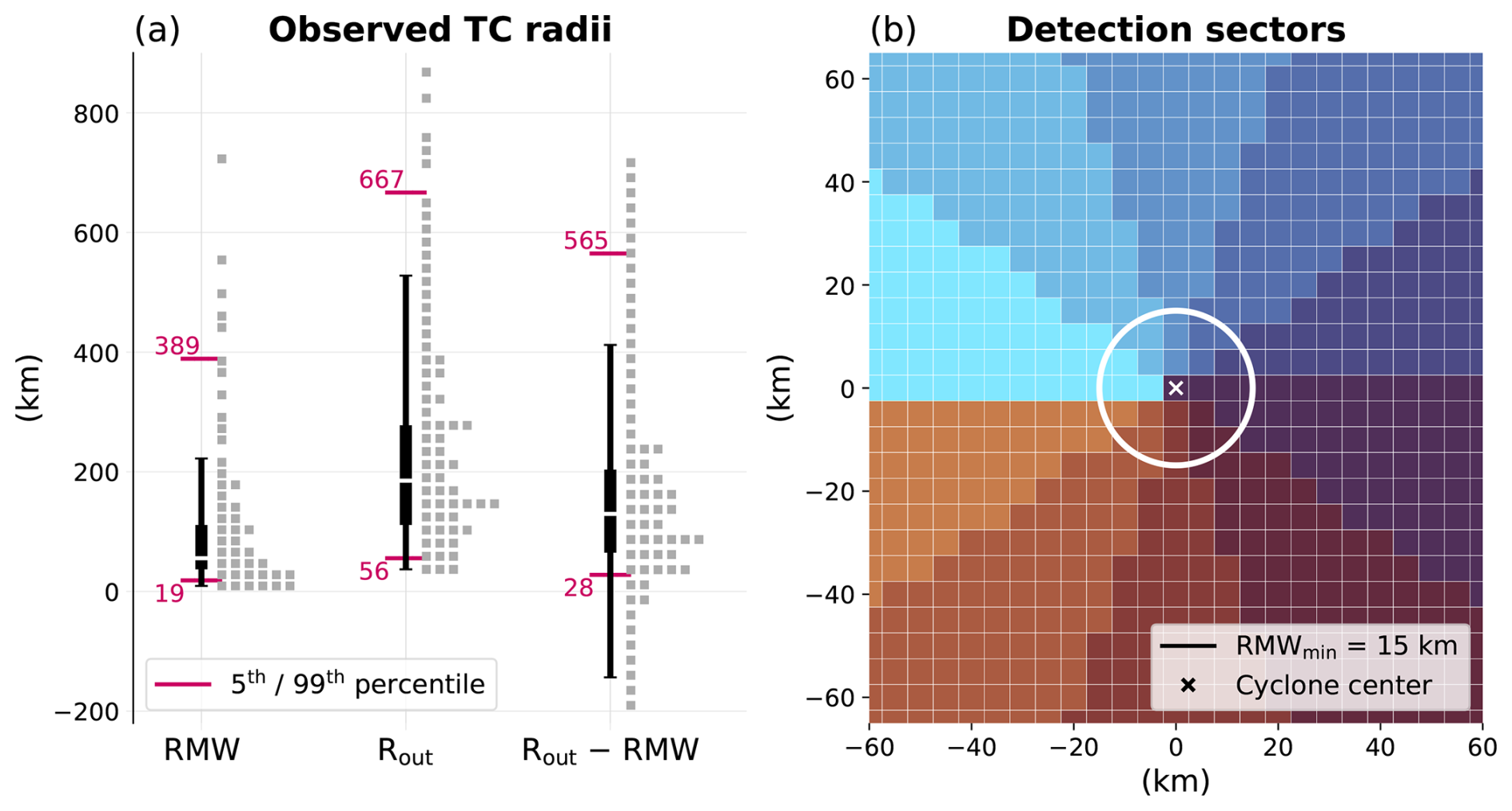
Figure B3 Box plots of observed RMW, R_out, and their difference (R_out-RMW) over the full life cycle of TCs (a), based on HURDAT2 data (since 2021, where RMW and R_out estimates are available). Gray squares to the right of each box plot represent 50/100/100 data points, respectively, to illustrate data distribution. Pink lines mark the 5th and 99th percentiles, asymmetrically chosen in the favor of the larger ones, since ICON tends to produce larger TCs than observed (Judt et al., 2021). For R_out-RMW, only positive values were considered to calculate the percentiles due to physical constraints. Schematic of the 10 detection sectors (blue to brown) on a 5 km grid (b). The TC center is marked by a white cross and the minimum RMW threshold of 15 km is shown as a white circle.

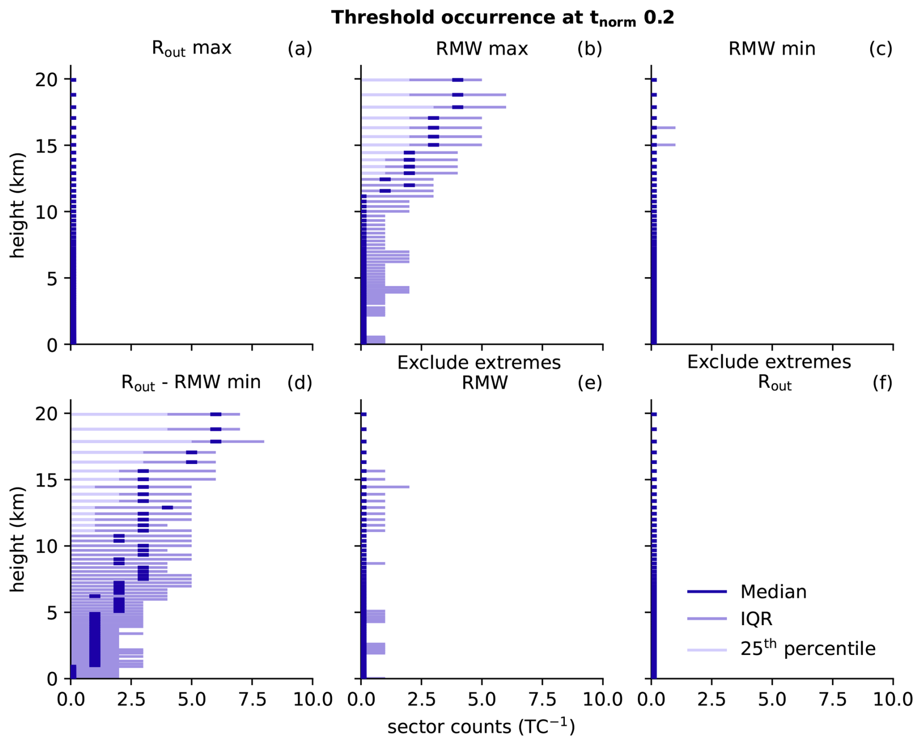
Figure B4 Occurrence of detection thresholds at early stage (t_norm = 0.2) of a TC: a maximum allowed vortex border R_out (a), maximum and minimum allowed RMW (b, c), minimal distance between R_out and RMW (d). Panels (e) and (f) indicate occurrences of extremes, which were excluded. For RMW/R_out a radius is excluded if it exceeds 300 %/600 % of the median, respectively. The occurrence is summed over the 10 detection sectors for each TC. The 25th percentile of the counts over all the simulated TCs (light violet), the median (dark violet) and the IQR (medium light violet) are displayed to illustrate the occurrence distribution of the thresholds.

Figure B5 As in Fig. B4, but for maximum intensity (t_norm = 0.5).

Figure B6 As in Fig. B4, but for a late stage (t_norm = 0.8).

Appendix C: Unstructured storms

This section provides a few examples of the SyNC composites of less well structured storms. Figure C1 is the same cat_pres 5 TC as in Fig. 5, but at a moment briefly after storm genesis. Figure C2 shows the same weaker cat_pres 1 TC as in Fig. 6 but here at an early stage. In all storm snapshots, the eyewall is less clearly built up and the storm size is relatively small. Nevertheless, the algorithm manages to estimate the eyewall location and the overall storm extent. However, especially in the south-western quadrant, the distance between eyewall and storm border for both storms is relatively small, causing data extrapolation in the normalization process.

Figure C1 As Fig. 5, but short after genesis (t_norm = 0.05).

Figure C2 As Fig. 5, but for a cat_pres 1 storm short after genesis (t_norm = 0.05).

Appendix D: Composite comparison

Figures D1, D2, D3 and D4 provide a composite comparison of additional variables. Figure D1 illustrates the benefits of the SyNC composites for intense TCs. Figures D2 and D3 illustrate the benefits for weak TCs.

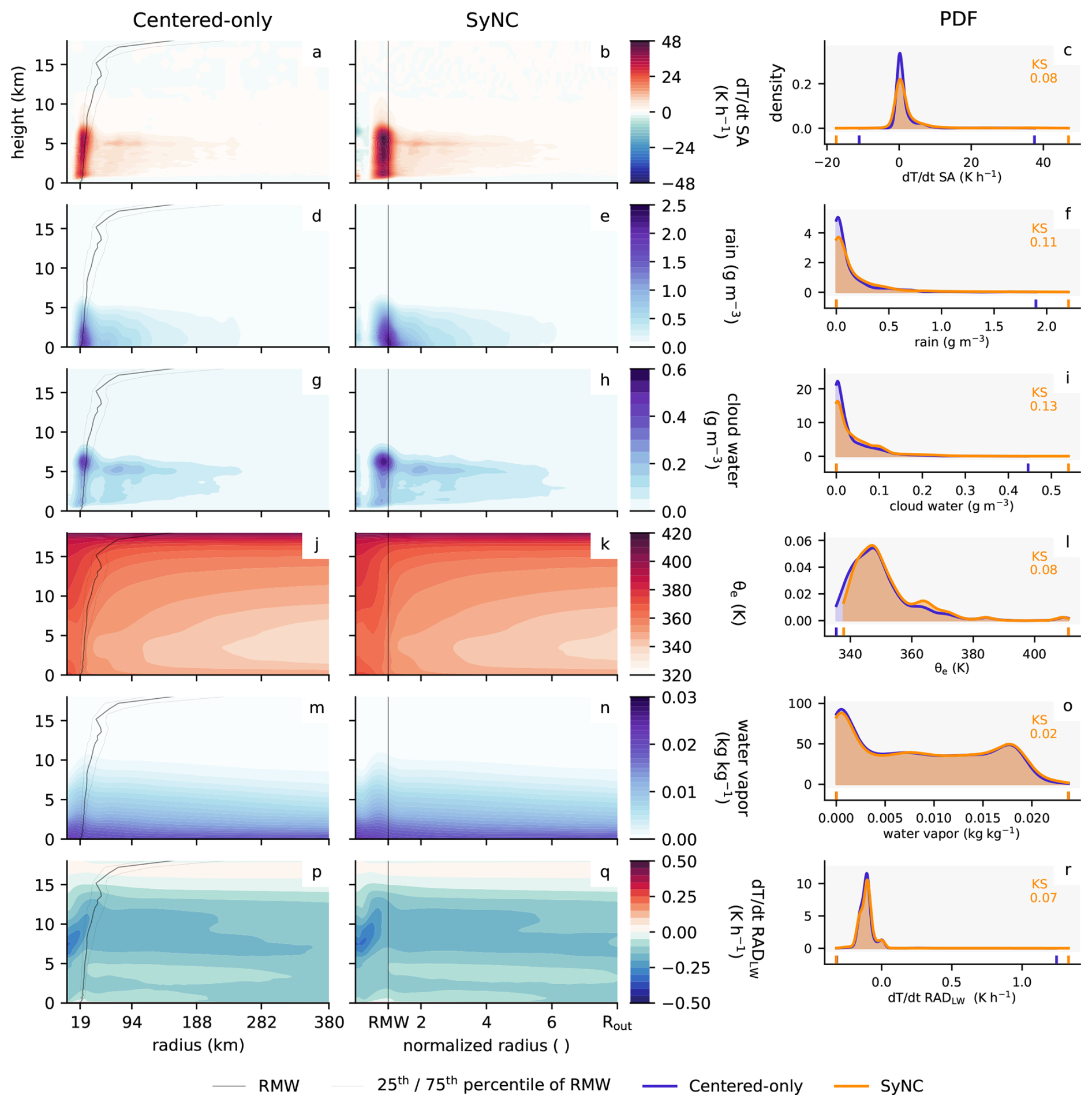
Figure D1 As Fig. 8, but for temperature tendencies due to saturation adjustment ($\mathrm{d}T/\mathrm{d}t$ SA, a–c), rain mass (d–f), cloud water (g–i), equivalent potential temperature (θ_e, j–l), water vapor (m–o) and temperature tendency due to longwave radiation emission (p–r).

Figure D2 As Fig. 8, but for weak storms (n = 15).

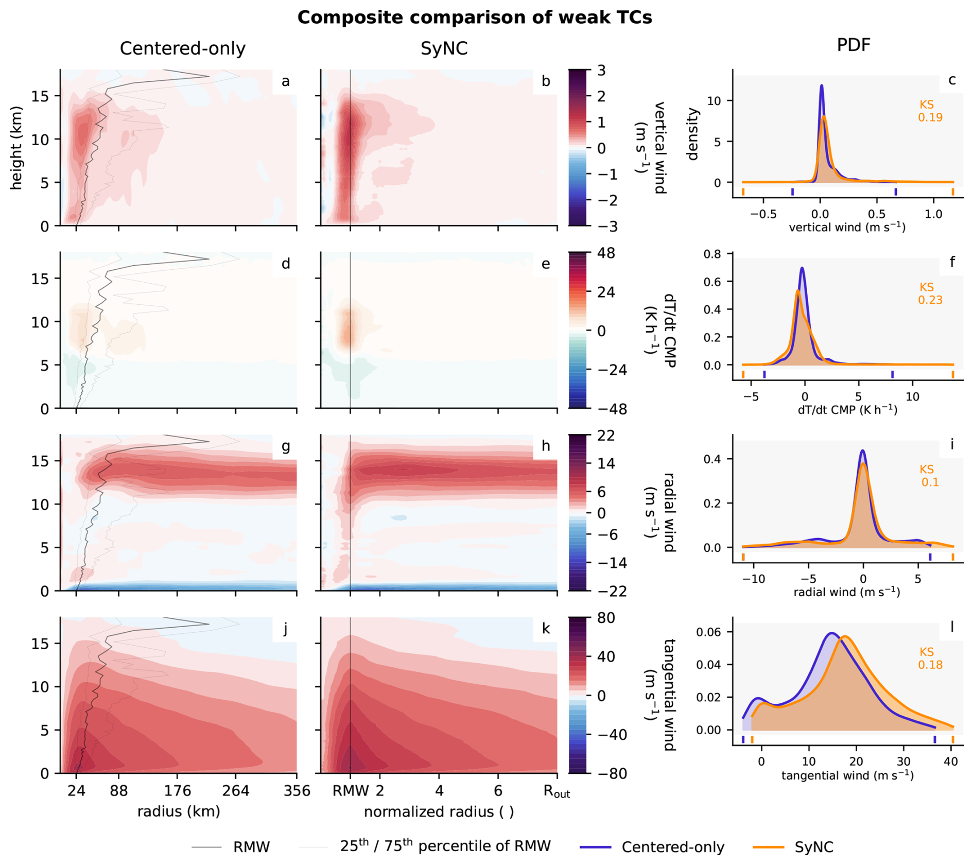
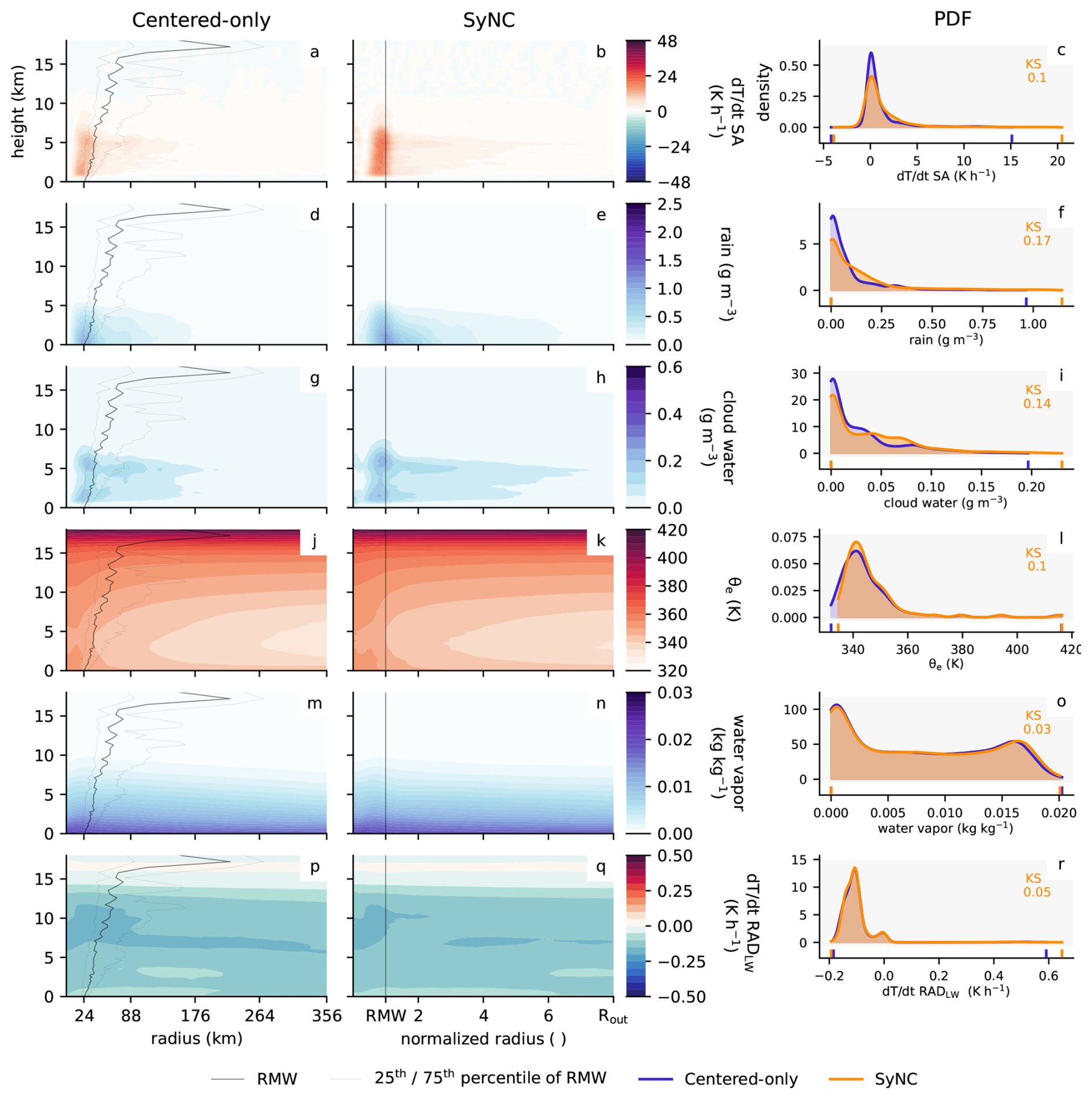
Figure D3 As Fig. 8, but for weak storms: temperature tendencies due to saturation adjustment ($\mathrm{d}T/\mathrm{d}t$ SA, a–c), rain mass (d–f), cloud water (g–i), equivalent potential temperature (θ_e, j–l), water vapor (m–o) and temperature tendency due to longwave radiation emission (p–r).

Figure D4 As Fig. 9, but for weak storms (n = 15).