Iterative run-time bias corrections in an atmospheric GCM (LMDZ v6.3)

Run-time bias corrections of atmospheric circulation models can be based on nudging (Newtonian relaxation) to an atmospheric reanalysis. In this case, the time increments of selected state variables are modified by adding the nudging terms obtained with an uncorrected version of the model. This is a well-known method to improve the models' representation of large-scale circulation patterns. In this work, we propose and evaluate a variant of this method, consisting of iterative nudging: the corrected model is itself nudged towards the reanalysis, and the resulting nudging terms are added to the initial ones to calculate the new, iterated correction terms. This procedure can be iterated an arbitrary number of times. Evaluating the LMDZ atmospheric general circulation model (AGCM) for a varying number of iterations of nudging to the ERA5 reanalysis for the period 1981–2000, we show that the simulated large-scale circulation patterns over the period 2001–2020 are consistently improved when the bias correction procedure is iterated compared to the non-iterated original procedure. However, signs of over-correction appear after about three iterations.

1 Introduction

Despite constant and continuing progress over several decades, climate models (in a broad sense, ranging from Earth System Models to limited-area dynamical atmospheric circulation models) still exhibit biases in their representation of current climate and of large-scale indicators of climate change (Eyring et al., 2021; Arias et al., 2021). Nevertheless, in the face of rapid climate change and its increasingly detrimental impacts, climate models remain the primary source of information to quantify future climate change from global to regional scales (Lee et al., 2023). However, for most use cases, run-time bias corrections of climate models, or bias adjustments of their output, are necessary (Doblas-Reyes et al., 2021; Ranasinghe et al., 2021).

The type of empirical run-time bias corrections (ERBC) that is used in the present work has, to our knowledge, first been described for atmospheric general circulation models by Guldberg et al. (2005), building on earlier work with simplified models (D'Andrea and Vautard, 2000) that already contains the main ideas. In this approach, time increments to the model's state variables are corrected using terms derived from the corrected increments that are obtained using a simulation that is nudged to atmospheric analyses or, more frequently, reanalyses (see Sect. 2). A number of studies have used this approach, or slight variations thereof (e.g., Bloom et al., 1996), to reduce systematic model errors in a weather or seasonal prediction context (e.g., Kharin and Scinocca, 2012; Chang et al., 2019).

Nudging as such, without the additional ERBC step building on it, is a frequently used technique for climate model evaluation (e.g., Sun et al., 2019; Zhang et al., 2022; Pithan et al., 2023). Notably, despite the frequent use of nudging in climate models, the specific implementation strategy and parameter choices (in particular, the nudging strength) need to be carefully chosen and evaluated (e.g., Zhang et al., 2014).

Here we use the nudging-based ERBC approach to reduce climate model biases with the explicit intention to produce bias-corrected climate projections as, for example, in Krinner et al. (2019). In a perfect model framework, the nudging-based ERBC approach has been shown to substantially improve simulated future climate projections (Krinner et al., 2020). Together with the fact that even in the context of a strong climate change (4×CO₂), large-scale climate model bias patterns have been shown to be stationary to a high degree (Krinner and Flanner, 2018), this justifies the use of this method, for example, for projections of future Antarctic climate on a centennial time scale (Krinner et al., 2019; Beaumet et al., 2019). Compared to post-hoc bias adjustment of climate model output, a potential advantage of run-time bias corrections is that the improved large-scale circulation patterns can lead to a more physically consistent multivariate representation of climate change. Moreover, even if the output of a climate model using such a run-time bias correction method may require further statistical bias correction because necessarily some biases remain (e.g.,  Scinocca and Kharin, 2024), a better representation of large-scale circulation patterns may help avoid pitfalls of post-hoc statistical bias corrections linked to the misplacement of critical circulation features (e.g., Hall, 2014; Maraun et al., 2017).

Nudging-based run-time bias corrections only partly eliminate model biases. Root mean square error (RMSE) reductions of about 30 %–50 % are typical for this method (Krinner et al., 2020; Scinocca and Kharin, 2024), depending on the model and the assessed variable. This is the main reason why in this paper, we examine the question whether an iterative application of this method can lead to a more effective bias reduction. However, as with any model tuning or bias correction, care has to be taken to avoid over-correction of model biases. The aims of this paper are therefore (a) to describe the iterative bias correction procedure implemented in the LMDZ6 atmospheric GCM (Hourdin et al., 2020); (b) to evaluate the simulated present-day climate in the uncorrected model and for a varying number of iterations of the correction procedure; (c) to determine limits of the procedure, in particular by identifying possible signs of over-correction.

The next section describes the iterative run-time bias correction method and the simulations carried out to test it. We then present results for circulation-related variables on large spatial and varying temporal scales, and discuss the potential of the method and its limitations, as well as limitations of the present work.

2 Methods

2.1 Iterative run-time bias correction

We start from the “classical” nudging-based run-time bias correction method described by Guldberg et al. (2005). Following the notation used by Scinocca and Kharin (2024), the original model increments for a state variable X (e.g. the meridional or zonal wind component) are noted M(X,t):

$$\begin{array}{}\text{(1)}& {\partial }_{t}X=\mathrm{M}(X,t).\end{array}$$

When the model is nudged (Jeuken et al., 1996) to a (re)analysis, these time-varying model increments become:

$$\begin{array}{}\text{(2)}& {\partial }_{t}X=\mathrm{M}(X,t)+{\displaystyle \frac{X_{\mathrm{a}}-X}{\mathit{\tau }}}\equiv {\mathrm{N}}_{\mathrm{0}}(X,t),\end{array}$$

where X_a denotes the reanalysis state variable, τ the nudging timescale (here, 1 d), and N₀ the nudged version of the model. The influence and the choice of the nudging time constant is discussed in Sect. 4.2. The nudging strength is reduced to 0 near the surface (using a hyperbolic tangent factor transitioning from close to 1 to close to 0 over a range of about 500 m around 1500 m above the surface, and similarly at the upper limit of the atmosphere (beyond 5 hPa)).

The climatological nudging increments $G_{\mathrm{0}}=\stackrel{\mathrm{‾}}{(X_{\mathrm{a}}-X)/\mathit{\tau }}$ (the overbar denoting a cyclostationary time average, taking into account seasonal and daily cycles) are then used in a bias-corrected simulation denoted C₀:

$$\begin{array}{}\text{(3)}& {\partial }_{t}X=\mathrm{M}(X,t)+G_{\mathrm{0}}\equiv {\mathrm{C}}_{\mathrm{0}}(X,t),\end{array}$$

where G₀ is a function of space (latitude, longitude and vertical level) and time (day of the year). To reduce the high-frequency weather noise generated by averaging over only 20 years for any given day of the year, we apply a 20 d running-mean average to the final correction terms, but preserve the mean daily cycle.

Until this stage, this is, as stated, the “classical” run-time bias correction method described by Guldberg et al. (2005).

We can now simply iterate this procedure for a first time, using the initial corrected model C₀:

$$\begin{array}{}\text{(4)}& {\partial }_{t}X={\mathrm{C}}_{\mathrm{0}}(X,t)+{\displaystyle \frac{X_{\mathrm{a}}-X}{\mathit{\tau }}}\equiv {\mathrm{N}}_{\mathrm{1}}(X,t).\end{array}$$

Here, N₁ stands for the first iterated nudging. The cyclostationary climatological nudging increments $G_{\mathrm{1}}=\stackrel{\mathrm{‾}}{(X_{\mathrm{a}}-X)/\mathit{\tau }}$ of this first iteration are then added to the initial correction terms G₀: $G_{\mathrm{0}+\mathrm{1}}=G_{\mathrm{0}}+G_{\mathrm{1}}$. The first iterated corrected model run C₁ then uses these combined correction terms:

$$\begin{array}{}\text{(5)}& {\partial }_{t}X=\mathrm{M}(X,t)+G_{\mathrm{0}+\mathrm{1}}\equiv {\mathrm{C}}_{\mathrm{1}}(X,t).\end{array}$$

This iteratively corrected model can then again be nudged to the (re)analysis. In general terms, the nth iteration of the bias-corrected model is then given by:

$$\begin{array}{}\text{(6)}& {\partial }_{t}X=\mathrm{M}(X,t)+G_{\mathrm{0}+\mathrm{1}+\mathrm{\dots }+n}\equiv {\mathrm{C}}_n(X,t).\end{array}$$

Because the nudging timescale τ is of the order of days (here, 1 d) and the model timestep of the order of minutes, the initial correction term G₀ derived from Eq. (2) only partially offsets the model's systematic drift relative to the reanalysis. Similarly, the subsequent correction terms G₀₊₁ and more generally $G_{\mathrm{0}+\mathrm{1}+\mathrm{\dots }+n}$ only partially offset this systematic drift. The question of potential convergence is addressed in Sect. 3.1.

2.2 Simulations and analysis

We use the LMDZ6 AGCM (Hourdin et al., 2020) at low resolution (96 (longitude) × 95 (latitude) horizontal grid points and 79 vertical levels), coupled to the ORCHIDEE land surface model (Krinner et al., 2005). The model is nudged towards the ERA5 reanalysis (Hersbach et al., 2020) for the period 1981–2000 (plus the year 1980 for model spinup). Only the meridional and zonal wind components above about P=0.85P_s (where P and P_s are the atmospheric pressure at a given level and at the surface, respectively) are nudged towards ERA5 with a time constant of τ=1 d in the nudged simulations N_i (i=0…3). The corrected simulations C_i (i=0…3) and the uncorrected control simulations, denoted M, are run for the evaluation period 2001–2020 (plus the year 2000 for model spinup), distinct from the nudging period. These simulations are run twice, starting in 2000 with varying initial conditions. For these simulations we use atmospheric states obtained from other uncorrected LMDZ simulations for the years 1995 and 2000, respectively, and discard the first year of the integration as spinup, as just mentioned. The presented results for these simulations M and C_i are the average of these $\mathrm{2}\times \mathrm{20}=\mathrm{40}$ model years. Table 1 provides a summary of the simulations described in this work.

Table 1 Simulations discussed in detail in this work.

In the Discussion, we briefly refer to one additional iteratively bias-corrected, supplementary test simulation that uses a nudging timescale of τ=3 d.

Evaluation is carried out against 2001–2020 ERA5 circulation characteristics such as climatological mean biases for meridional (v) and zonal (u) wind at selected standard pressure levels (850, 500 and 200 hPa), mean sea-level pressure biases, interannual patterns of sea-level pressure variability using empirical orthogonal functions, blocking frequencies (Davini et al., 2012; Palmer et al., 2023) based on 500 hPa geopotential indices, band-pass (between 2.5 and 7 d) sea-level pressure variability linked to storm track location and intensity (Chang, 2009), and frequencies of synoptic weather patterns using 5×4 self-organizing maps (Kohonen, 1982) of hemispheric extratropical (polewards of 40° N and S) daily-mean geopotential heights. Furthermore, the amplitude of the u and v correction terms is analyzed to evaluate convergence of the correction procedure.

Contrary to previous studies (Krinner et al., 2019, 2020), we refrained from bias-correcting atmospheric temperatures because we have realized that run-time temperature bias corrections in the LMDZ AGCM destructively interfere with the physical parameterizations in the tropics. In particular, the temperature corrections significantly reduce a large-scale tropospheric cold bias in the model, leading to reduced convective instability and thus to reduced simulated convective activity, accumulation of water vapour in the atmospheric boundary layer, and a substantial surface energy flux imbalance linked to reduced surface evaporation and increased downwelling longwave radiation.

3 Results

3.1 Nudging and correction increments

The amplitude of the nudging increment decreases for higher iterations, as shown in Fig. 1 for the zonal mean absolute zonal wind nudging increments. While the spatial patterns are broadly similar for all simulations N_i, the amplitude of the nudging increments decreases by approximately a factor of 2–3 from N₀ to N₃. Contrary to the nudging increments, which decrease, the amplitude of the bias correction increments applied in simulations C_i increases for higher iterations, as the correction increments $G_{\mathrm{0}+\mathrm{\dots }+i}$ for simulation C_i are the sum of the average nudging increments of N₀ to N_i (see Eq. 6). The spatial structure of the bias correction increments $G_{\mathrm{0}+\mathrm{\dots }+i}$ also remains similar for the successive iterations C_i, but for the higher iterations it is not a simple spatially constant multiple of the initial correction increments G₀ used for C₀, as shown by the ratio of the zonal mean absolute zonal wind correction increments between $G_{\mathrm{0}+\mathrm{\dots }+\mathrm{3}}$ and G₀, displayed in Fig. 2. Instead, this ratio has distinctive spatial structures varying in space and in time through the annual cycle (not shown), indicating that the iterative procedure is not identical to a simple uniform amplification of the initial correction. We interpret this as being linked to the non-linear and non-local nature of the atmospheric system, where the bias corrections implemented during a correction step can increase tendency errors elsewhere, which are then corrected during the next iteration, and where spatially unequal bias reduction at one iteration can also lead to modified tendency errors, and thus subsequent bias reduction, in the following iteration.

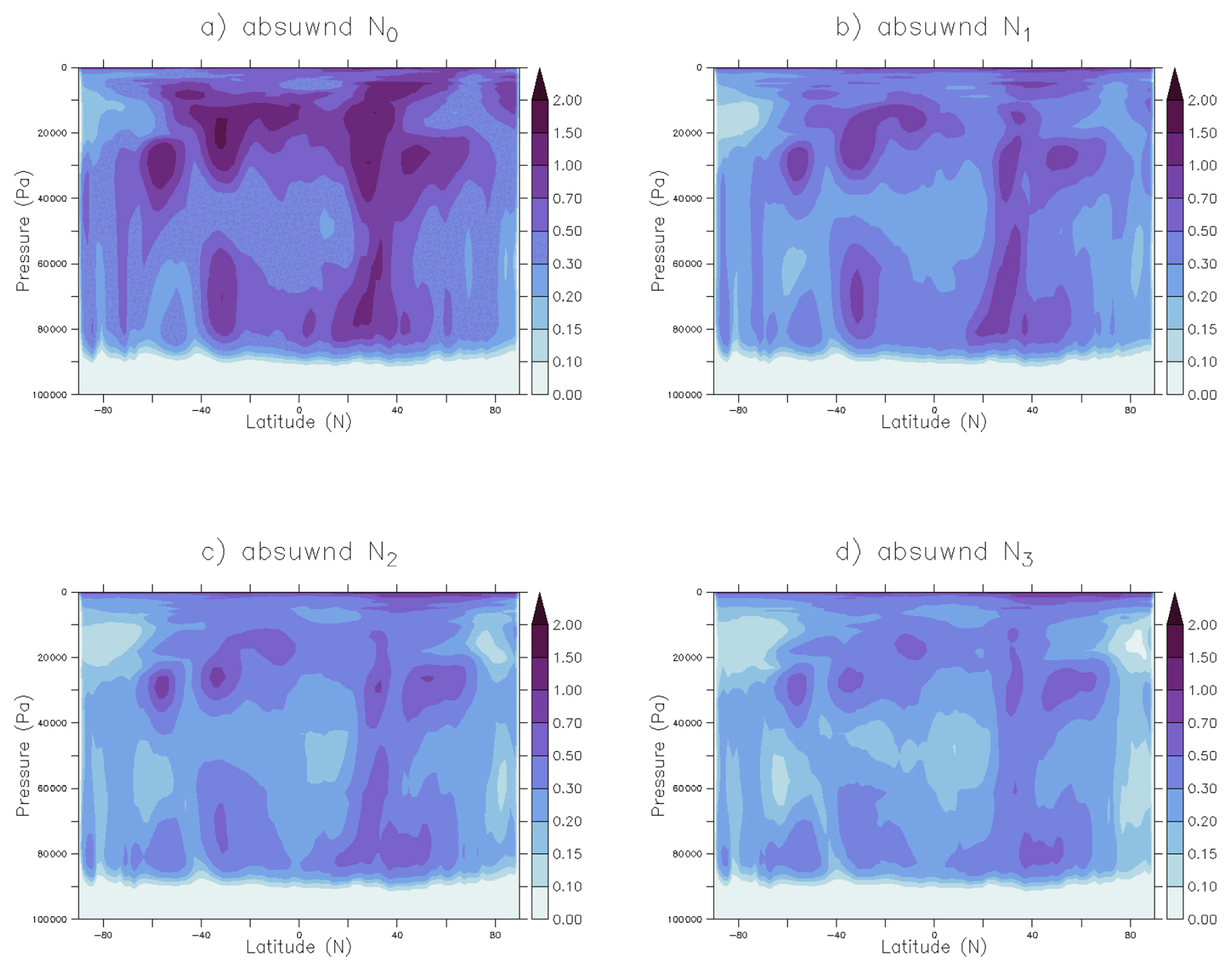
Figure 1 Zonal mean absolute zonal wind nudging increments (in $\mathrm{m}{\mathrm{s}}^{-\mathrm{1}}{\mathrm{d}}^{-\mathrm{1}}$) calculated from (a) N₀ (used in C₀); (b) N₁; (c) N₂; (d) N₃, average for January 1981 to 2000.

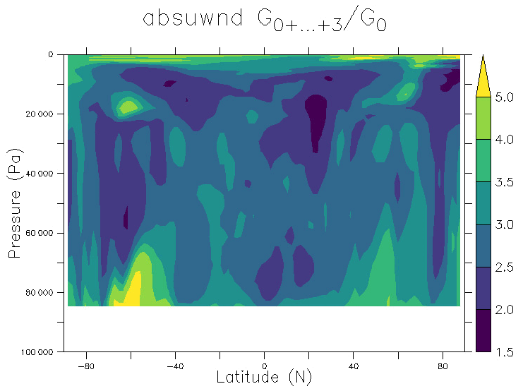
Figure 2 Ratio of the zonal mean absolute zonal wind bias correction terms (averages for January 1981 to 2000) between those used in C₃ (bias correction terms $G_{\mathrm{0}+\mathrm{\dots }+\mathrm{3}}$) and those used in C₀ (bias correction terms G₀). Values between 100 000 and 85 000 Pa are not shown in the lower part of the figure. They are not relevant as, by construction, the absolute values of the increments vanish at these altitudes (see Fig. 1).

Do these successive correction terms converge towards some “final” correction term? Figure 1d shows that the nudging increments in the third iterated nudging step N₃ do not vanish, although they are substantially weaker than in N₀ (Fig. 1a). The global mean of the absolute zonal wind nudging tendencies (in January, to be consistent with Fig. 1) is 0.50 $\mathrm{m}{\mathrm{s}}^{-\mathrm{1}}{\mathrm{d}}^{-\mathrm{1}}$ for N₀, 0.35 $\mathrm{m}{\mathrm{s}}^{-\mathrm{1}}{\mathrm{d}}^{-\mathrm{1}}$ for N₁, 0.29 $\mathrm{m}{\mathrm{s}}^{-\mathrm{1}}{\mathrm{d}}^{-\mathrm{1}}$ for N₂, and 0.26 $\mathrm{m}{\mathrm{s}}^{-\mathrm{1}}{\mathrm{d}}^{-\mathrm{1}}$ for N₃. This means that the intensity of the remaining nudging tendencies decreases at higher iterations, but convergence towards potentially vanishing final nudging tendencies is still far away after 3 iterations. The combined correction terms arising from the sum of these absolute zonal wind nudging tendencies have global mean values of 0.50 $\mathrm{m}{\mathrm{s}}^{-\mathrm{1}}{\mathrm{d}}^{-\mathrm{1}}$ for G₀ (because G₀ is identical to the mean nudging tendencies of N₀), 0.83 $\mathrm{m}{\mathrm{s}}^{-\mathrm{1}}{\mathrm{d}}^{-\mathrm{1}}$ for G₀₊₁, 1.09 $\mathrm{m}{\mathrm{s}}^{-\mathrm{1}}{\mathrm{d}}^{-\mathrm{1}}$ for $G_{\mathrm{0}+\mathrm{1}+\mathrm{2}}$, and 1.30 $\mathrm{m}{\mathrm{s}}^{-\mathrm{1}}{\mathrm{d}}^{-\mathrm{1}}$ for $G_{\mathrm{0}+\mathrm{\dots }+\mathrm{3}}$, and are thus somewhat lower than the corresponding sums of the global mean of the absolute zonal wind nudging tendencies (which would be 0.5, 0.85, 1.14 and 1.40 $\mathrm{m}{\mathrm{s}}^{-\mathrm{1}}{\mathrm{d}}^{-\mathrm{1}}$, respectively), indicating that some local-scale compensation occurs between different iterations, as already shown by Fig. 2.

3.2 Mean errors

Plots for wind bias reductions obtained with the standard bias correction method and its successive iterations are provided in Fig. 3 (maps for u at 500 hPa) and in Fig. 4 (zonal means for u and v). Figure 3 displays the 1981–2000 annual mean bias of the zonal wind component at 500 hPa for the different simulations. Figure 4 displays, in each of its two panels, the ratio of the 1981–2000 RMSE in each of the corrected simulations C_i ($i=\mathrm{0},\mathrm{\dots },\mathrm{3}$) and the RMSE of the uncorrected control simulation M: RMSE(C_i)$/$RMSE(M), for the annual mean of the zonal (a) and meridional (b) wind speed, where the RMSE is calculated with respect to ERA5.

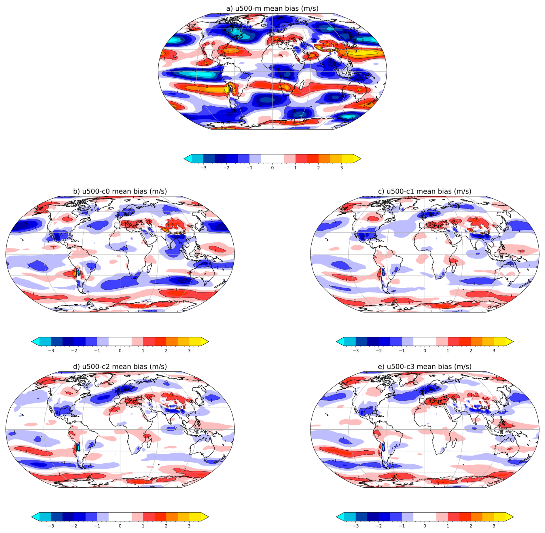
Figure 3 Annual mean 500 hPa zonal wind mean bias with respect to ERA5 (in m s⁻¹), for different simulations. (a) Uncorrected control simulation M; (b) corrected simulation C₀; (c) first iterated corrected simulation C₁; (d) second iterated corrected simulation C₂; (e) third iterated corrected simulation C₃.

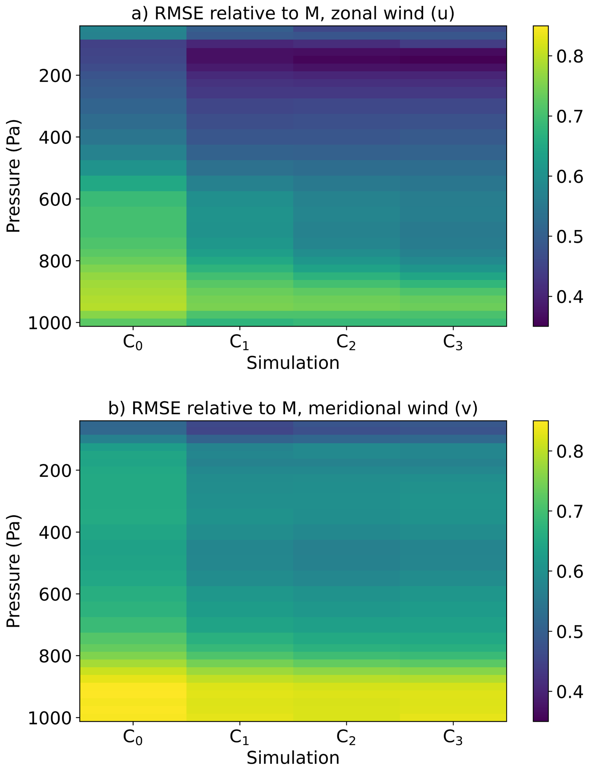
Figure 4 Annual mean of monthly mean RMSE (with respect to ERA5) for zonal (a) and meridional (b) wind, for the corrected simulations C₀–C₃, relative to the same quantity for the uncorrected control simulation M. Values below 1 indicate that the RMSE in the corrected simulations C_i is smaller than the RMSE of the uncorrected control simulation M.

By construction, mean wind biases at various levels in the atmosphere are decreased in the corrected simulation C₀ compared to the uncorrected control simulation M. Relative to M, the RMSE of the zonal and meridional wind components u and v is decreased by ≈20 % near the atmospheric boundary layer (where no correction is applied) to ≈60 % (for u) at 200 hPa. When the correction procedure is iterated once (simulation C₁), a further substantial RMSE reduction is obtained. In most cases except close to the atmospheric boundary layer, no substantial further improvement is obtained in subsequent iterations of the correction procedure.

In the absence of run-time temperature corrections in this study, substantial large-scale air temperature biases remain in our wind-only corrected simulations C_i (see Fig. 5). While the wind corrections lead to improvements in the zonal-mean temperature simulation in the upper atmosphere, above ≈300 hPa, the bias reduction is only modest below this level. In addition, further bias reduction between 200 and 300 hPa in polar regions during higher iterations (>2) of the bias correction procedure come at the expense of a degradation of the simulated temperature patterns at these latitudes at about 150 hPa. Because the wind corrections act through the model dynamics, its influence on temperature is expected to arise primarily through dynamical balance (e.g. thermal wind, geostrophic and hydrostatic adjustment), which constrains horizontal temperature gradients rather than the global-mean temperature at a given pressure level. As a result, wind-only bias correction can reasonably be expected to improve regional temperature anomalies about the level-wise global mean while leaving the global-mean temperature largely unaffected, since the latter is controlled by the column-integrated energy balance and model physics. Therefore, when for a given pressure level the global mean bias is accounted for (i.e. subtracted, yielding a centered temperature $\stackrel{\mathrm{̃}}{T}=T-\mathrm{\Delta }T$, where ΔT is the global mean temperature bias at a given atmospheric level), the remaining regional bias patterns are reduced in the corrected simulations except very close to the surface, as can be seen in Fig. 6 that displays the RMSE of this centered temperature $\stackrel{\mathrm{̃}}{T}$. In this case the iterative run-time bias correction procedure leads to further improvement in most parts of atmosphere above about 900 hPa (with the exception of a small degradation of the biases at about 850 hPa, which are already not well corrected in C₀, and an already-mentioned degradation at about 150 hPa). This means that, while the global mean temperature biases – predominantly cold below about 150 hPa and very likely caused by deficiencies in the model physics – are not corrected, regional-scale temperature bias patterns are smoothed because of the corrected model dynamics.

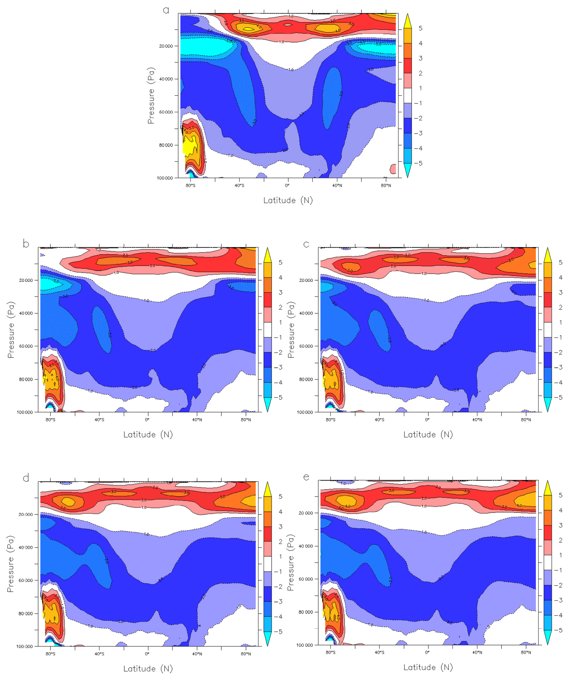
Figure 5 Zonal and annual mean temperature biases of the control simulations M (a) and the corrected simulations C₀–C₃ (b–e) against ERA5 (°C).

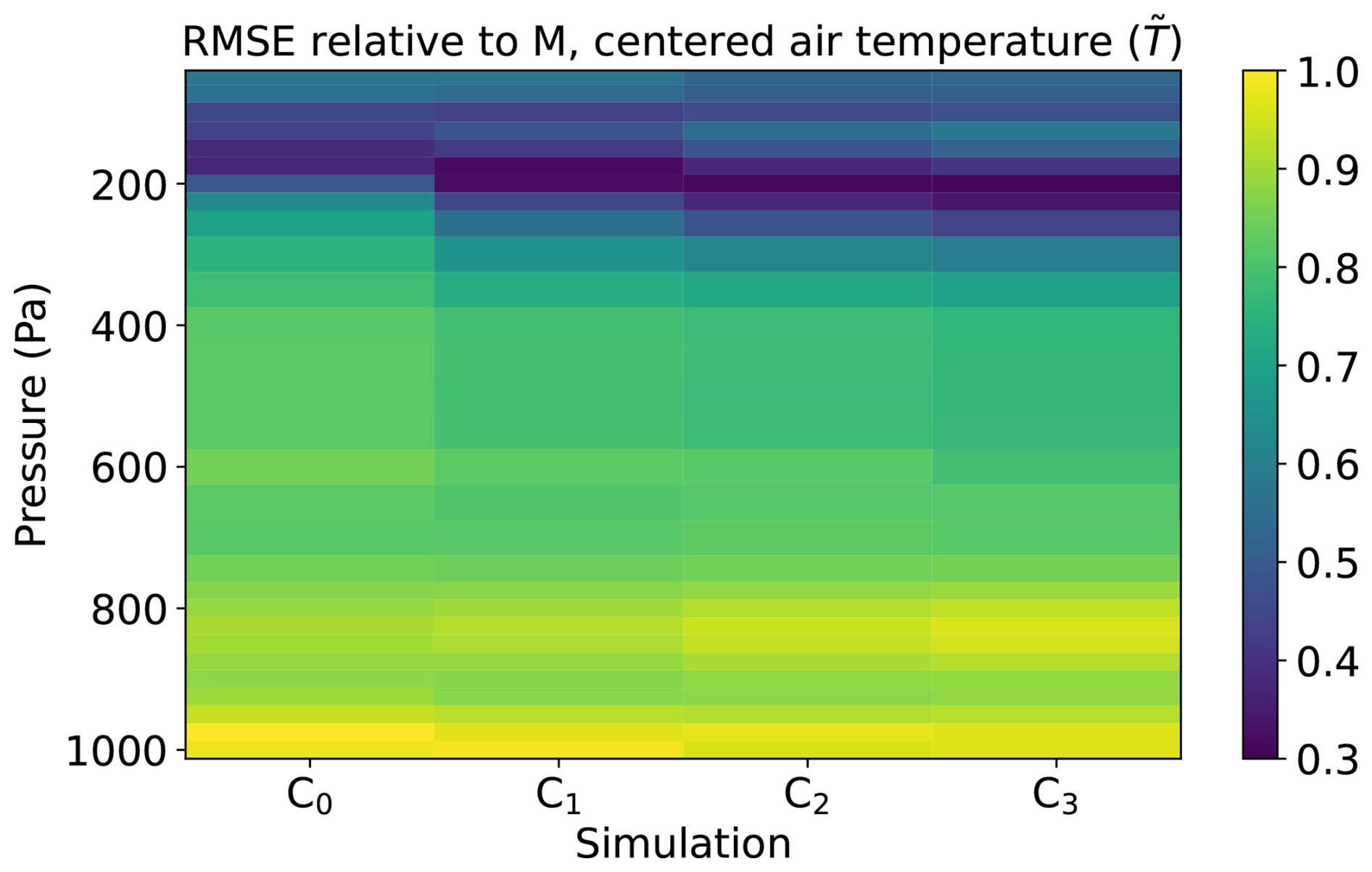
Figure 6 Annual mean of monthly mean RMSE (with respect to ERA5) of the centered air temperature $\stackrel{\mathrm{̃}}{T}$ (see text), for the corrected simulations C_0…3, relative to the same quantity for the uncorrected control simulation M, with global mean bias for the respective level subtracted. Values below 1 indicate that the RMSE in the corrected simulations is smaller than the RMSE of the uncorrected control simulation.

Sea-level pressure biases are only weakly reduced in our simulations that only bias-correct wind patterns. In C₀, the global RMSE of the annual mean sea-level pressure (with respect to ERA5) is reduced by 10 % compared to the uncorrected control simulation M, and iterations of the bias correction method only lead to insignificant overall improvements (the reduction compared to M is 13 % for simulation C₃). The weak correction of sea-level pressure errors is in contrast to earlier results for the Southern Hemisphere obtained using run-time temperature corrections (Krinner et al., 2019).

3.3 Monthly to interannual circulation variability

As stated, building on cyclostationary correction terms, the run-time bias correction procedure used here is, by construction, designed to better represent climatological mean values of the corrected variables. However, it is certainly of equal importance to assess whether these run-time bias corrections also improve the way the model represents circulation variability on different timescales.

The dominant patterns of interannual variability of monthly circulation structures are indeed more realistically depicted in the corrected simulations C₀ than in the uncorrected control simulations M, and even more so in simulations with iterated run-time bias corrections (C₁₋₃). This can be seen in Table 2 that displays the seasonal squared spatial Pearson correlation coefficient r² between simulated (LMDZ) and “observed” (ERA5) dominant modes of monthly 500 hPa geopotential anomalies, as identified by principal component analysis for the different corrected model runs C_i, relative to the corresponding squared spatial correlation coefficient for the uncorrected control simulations M: $R=r_{{\mathrm{C}}_i}^{\mathrm{2}}/r_{\mathrm{M}}^{\mathrm{2}}$.

Table 2 Squared spatial correlation coefficient r² between the corrected LMDZ runs C_i ($i=\mathrm{0},\mathrm{\dots },\mathrm{3}$) and ERA5, for the first EOF of monthly extratropical (30–90° latitude) variability of the 500 hPa geopotential height (ϕ_500 hPa) for selected seasons and hemispheres, 2001–2020, relative to the corresponding squared correlation coefficient $r_{\mathrm{M}}^{\mathrm{2}}$ of the uncorrected control simulation M: $R=r_{{\mathrm{C}}_i}^{\mathrm{2}}/r_{\mathrm{M}}^{\mathrm{2}}$. Only cases for which the variance explained in the ERA5 reanalysis exceeds 40 % are shown. The squared spatial correlation coefficient for the uncorrected control simulation M, $r_{\mathrm{M}}^{\mathrm{2}}$, is given in the last column for reference. The corrected simulation with the highest relative r² is bolded (although differences between simulations are not necessarily significant).

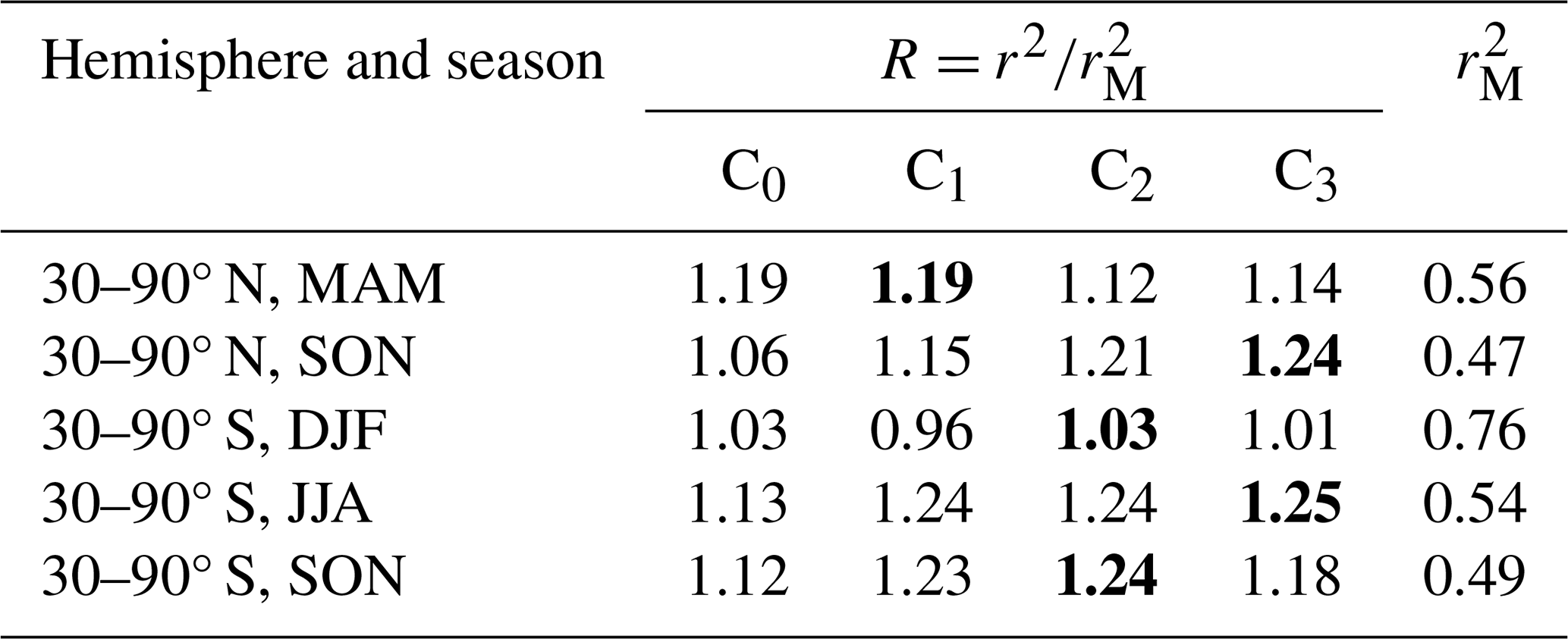
Only seasons for which the first principal component explains more than 40 % of the variance in the ERA5 dataset are retained here in order to restrict the analysis to the most stable and physically meaningful patterns. Although the 20-year observational period might be a bit short and could be the reason for some remaining noise in the results reported in Table 2 – the tendencies for a given season and hemisphere from C₀ to C₃ are not always steady –, it seems that an iteration of the run-time bias correction leads in most cases to a better representation of the interannual circulation variability patterns. The results reported here are obtained for the total 40 years of the two 20-year runs of each experiment C_i, but the results for individual 20-year runs of these experiments are very similar, increasing the confidence in the robustness of the results. Furthermore, the squared correlation coefficients overall increase between C₁ and C₂.

3.4 Short-term circulation variability

Diagnostics of short-term atmospheric circulation variability indicate an overall positive impact of the wind-based bias corrections for spatial means of bandpass-filtered extratropical winter sea-level pressure variability and average blocking frequencies (Table 3), but there is no clear improvement over multiple iterations of the correction procedure.

Table 3 RMSE of selected model results, calculated with respect to ERA5 (2001–2020) and normalized with respect to the uncorrected control simulations M, for high-frequency circulation-related quantities. σ_2.5–8 d (p_msl): bandpass-filtered (between 2.5 and 8 d) sea-level pressure standard deviation between 40 and 60° latitude in both hemispheres, limited to grid points below 1000 m surface height; f_B: annual mean frequency of blocking situations (based on daily mean 500 hPa geopotential height) between 30 and 75° N and S; f_S: individual frequencies of the 20 most representative hemispheric extratropical large-scale synoptic situations based on daily 500 hPa geopotential maps. The simulation with the lowest RMSE of the corrected simulations is bolded (note however that values >1 indicate that the model performance is degraded with respect to the uncorrected control simulations M). Differences between simulations are not necessarily significant.

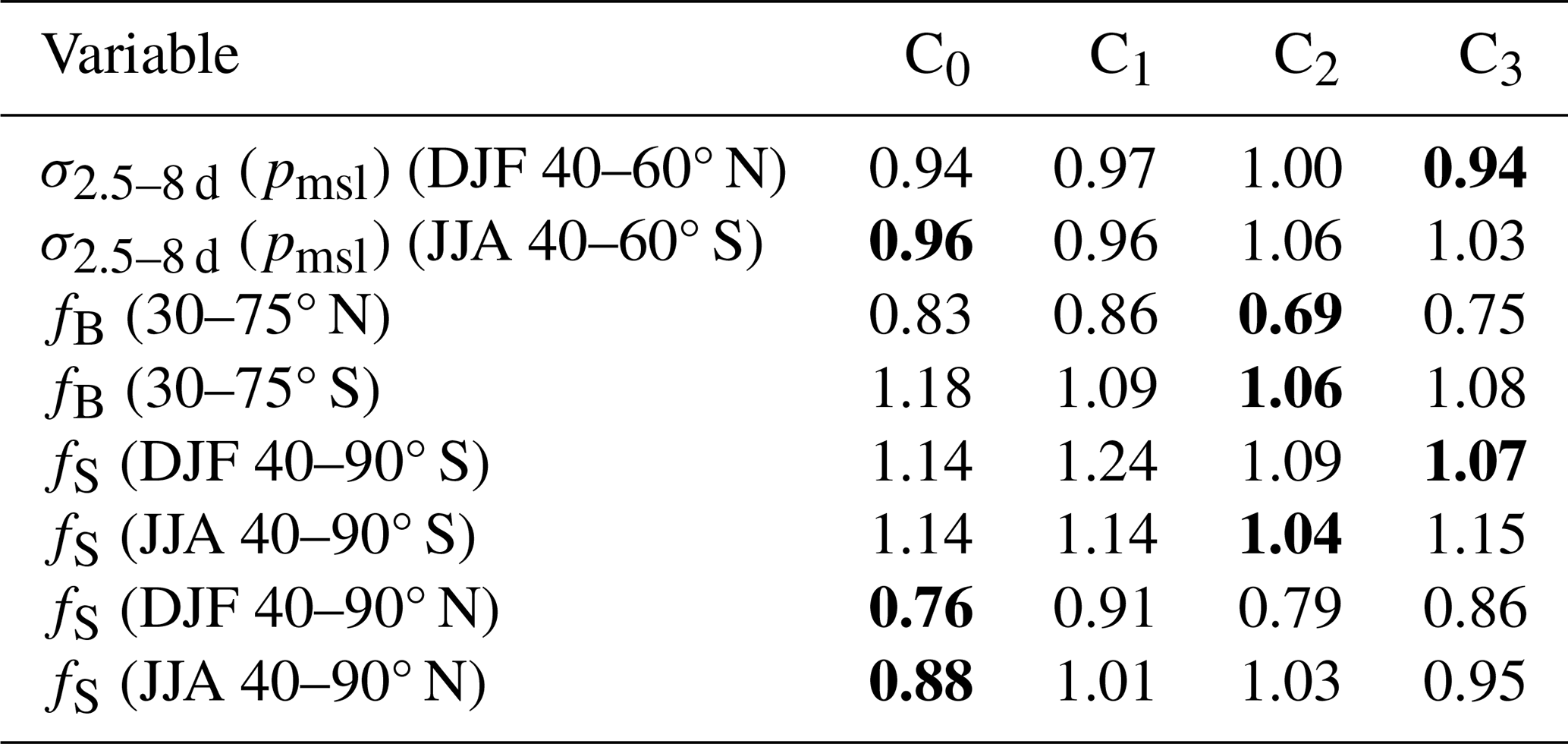
The winter short-term (2.5–8 d) mid-latitude (40–60° N and 40–60° S) sea-level pressure variability, diagnosed from the temporal standard deviation of sea-level pressure from its seasonal mean (σ_2.5–8 d, using a bandpass filtering in the frequency domain, and limited to grid points with surface height below 1000 m) shows no consistent improvement, and even slight degradation, for the iterated corrections C_1…3 compared to the simple non-iterated bias correction applied in C₀. However, the short-term pressure variability is overall better depicted in the corrected than in the uncorrected control simulations.

Blocking anticyclones are a significant atmospheric phenomenon, although there is not one standard accepted definition (Lupo, 2021). Here we follow the widely used definition by Davini et al. (2012): Blocking events are diagnosed at a given point in time and space based on the reversal of the meridional gradient of geopotential height measured at 500 hPa, extending over at least 15° of continuous longitude, and persisting within a 5° latitude × 10° longitude box centered on a given grid point for at least 5 d. We then calculate the annual mean frequency of these events for each grid point, and calculate the spatial RMSE E of these frequencies compared to ERA5. For each corrected simulation, the ratio between $E_{{\mathrm{C}}_i}$ for that simulation and E_M of the uncorrected control simulation is then computed, yielding a score $f_{\mathrm{B}}=E_{{\mathrm{C}}_i}/E_{\mathrm{M}}$. While the iterated procedure seems to improve the model score for the 30–75° N annual and spatial mean blocking frequency, (i.e., f_B (30–75° N) <1), with best results obtained for 2 and 3 iterations, the bias-corrected simulations show degraded performance compared to the uncorrected control simulations (i.e., f_B (30–75° S) >1) in the Southern Hemisphere (30–75° S). However, in the Southern Hemisphere, the iterated bias correction procedure leads to less degraded performance compared to a single bias correction in C₀.

In the Southern Hemisphere, the mean RMSE of the frequencies of typical hemispheric-scale daily circulation patterns, as identified using 20 (5×4) self-organizing maps for each season (DJF and JJA) and denoted as f_S in Table 3, is slightly degraded in the corrected simulations compared to the uncorrected control simulation (see f_S for 40–90° S in the table). Frequency errors are increased by about 15 % on average compared to the uncorrected control simulation. Iterations of the bias correction procedure (C_1…3) do not show any consistent change (neither improvement nor degradation) compared to the non-iterated bias correction applied in C₀, even if C₂ and C₃ show the least degradation in JJA and DJF, respectively, compared to C₀. In the Northern Hemisphere, the non-iterated bias correction C₀ procedure produces the best results of all simulations (including the uncorrected control simulation M). In other words, while the bias correction method appears to improve the model performance in this particular respect, iterating the bias correction procedure does not lead to further improvement of the frequency of the simulated main synoptic weather patterns (see f_S for 40–90° S in the table).

Overall, taking these diagnostics together, the wind bias correction does lead to a modestly improved representation of short-term atmospheric circulation variability, but iterating the bias correction procedure does not necessarily lead to clear further improvement. We note that in the cases where the model performance is degraded by applying the bias correction once (that is, C₀ shows degraded performance relative to M), iterating the bias correction can lead to improved (less degraded) results.

4 Discussion

4.1 Limitations linked to the design of the model simulations

4.1.1 Simulation periods: Length of the calibration and evaluation periods

We made the choice in this study to calibrate the bias-correction terms over the 1981–2000 period and to evaluate the effect of the bias correction for the out-of-sample period 2001–2020. This means that both periods only cover 20 years, albeit with two model realizations for the evaluation runs. Although 20 years is today often considered to be a reasonably long evaluation period – see for example the IPCC AR6 WGI model evaluation chapter (Eyring et al., 2021) –, one might wonder whether a longer calibration period would lead to substantially different results. However, there is a definite risk of over-correction when too long a calibration period is used, if only because this limits the possibility for out-of-sample testing. Of course this does not mean that a longer calibration period of 30 years would not be preferable when applying this method, as long as the conclusions for the experiment setup that have been drawn here with clear out-of-sample evaluation are kept in mind.

4.1.2 Model resolution

These simulations have been carried out at a rather low horizontal resolution of 3.75° (longitude) × 1.875° (latitude), lower than the standard IPSL-CM6A-LR setup used in CMIP6 (Bonnet et al., 2021) with its 2.5° × 1.25°. However, the vertical resolution, with 79 levels, corresponds to the standard CMIP6 setup for this model in order to reduce the need for re-tuning of the physical parametrisations. The reason for this choice is of course computational efficiency. Many model biases have similar structures at varying resolution, even if their amplitude can vary. The point here is to evaluate the benefit of iterated run-time bias corrections, rather than an optimum model setup with as weak as possible initial model biases. We are therefore fairly confident that our main results and conclusions remain valid at a higher horizontal resolution.

4.1.3 Choice of bias-corrected variables

Focusing on polar regions (Krinner et al., 2019), previous studies with empirical run-time corrections of wind and temperature in the LMDZ AGCM have yielded promising results. However, at least with the most recent version of the LMDZ AGCM, we have found strong detrimental effects of temperature corrections in the lower latitudes. As shown in Fig. 5, LMDZ has a wide-spread cold bias of about 2 °C in the mid-troposphere. Empirical run-time corrections of this bias physically correspond to an additional radiative heating. As mentioned before (Sect. 2), we suspect that this leads to a weakening of the temperature lapse rate and reduced convective activity. As a result, humidity accumulates in the lower troposphere, which reduces the upwards surface latent heat flux on large scales, in particular over the oceans, and the (approximate) global surface energy balance is strongly perturbed – in an ocean-atmosphere coupled model, this would lead to a very strong oceanic warming exceeding by far the observed oceanic heat uptake (von Schuckmann et al., 2023).

It is noteworthy that this destructive effect of empirical temperature correction is highly model-dependent. For example, no such effect has been noted in various versions of the Canadian atmospheric model CanAM (Krinner et al., 2020; Scinocca and Kharin, 2024). It is very likely that the package of physical parameterizations in LMDZ causes this cold bias, and at the same time counteracts temperature ERBC because it was consistently developed and tuned to comply with a certain set of observed metrics, on particular TOA radiative fluxes (Hourdin et al., 2021). In this model, complying with these radiative metrics appears to be in contradiction with an absence of a pervasive cold bias in the mid-troposphere, as tests of tuning strategies to eliminate the cold bias did not yield satisfying results in terms of TOA radiative metrics. We have to leave this problem unsolved for future work.

This motivated the choice to only bias-correct the wind in this study. As a consequence, as shown above, the widespread cold bias in the mid-troposphere is not corrected. Of course this raises questions about the usefulness of such bias-corrected simulations for driving limited-area models for simulations of the present climate and projections. The uncorrected large-scale cold bias of LMDZ would certainly also lead to a cold bias in the nested limited-area model which would, in most cases, not be able to correct for the bias through its own, possibly less biased, radiative-convective process representations, given the time scales of atmospheric circulation involved (see Labonté et al., 2025; Scinocca et al., 2025). If the aim of the bias-corrected simulations is to serve as boundary conditions for a regional climate model, then the relevant criterion will be the quality of the lateral boundary conditions (u, v, T, q) provided to the regional model rather than the internal physical behaviour of the global model, justifying temperature ERBC in LMDZ in spite of perturbed physics. But the aim of the present paper is to present the iterative ERBC method as such. Therefore, we limited the ERBC here to the zonal and meridional wind components.

The choice to only correct the horizontal wind components, and not other variables such as temperature or atmospheric humidity, can make sense if one thinks of the partly conceptual separation between model dynamics and physics. The horizontal wind components, in particular above the atmospheric boundary layer, are quite directly determined by the model dynamics. Atmospheric temperature and humidity, in contrast, and in particular on large spatial scales, can be seen as primarily determined by the model physics. One can argue that the pervasive cold bias throughout the almost entire mid-troposphere, partly “hidden” by stronger local temperature biases caused e.g. by the latitudinal misplacement of jet streams, should be preferably corrected by improved model physics or specific tuning. In contrast, localized biases caused by the misplacement of circulation features are often resolution-dependent and as such more obvious aims for empirical run-time bias corrections limited to the horizontal wind components. It can therefore make sense to separate atmospheric circulation structures from other variables such as temperature and humidity in bias-correction approaches. The effect of misplaced circulation features (for example, a misplaced storm track) often cannot be corrected a posteriori (see an example by Maraun et al., 2017), while a posteriori bias corrections of “physical” variables related to surface climate, such as temperature and precipitation, are quite usual.

4.2 Effect of the nudging time constant τ

In studies using the nudging technique, the optimal choice of the nudging time constant τ, and more generally of technical choices in the implementation of the nudging procedure, has repeatedly been the object of attention (e.g., Kruse et al., 2022; Zhang et al., 2022; Scinocca and Kharin, 2024). Tests of a range of different nudging time constants τ within the rather usual range between 1 and 3 d, both for the non-iterated and the iterated bias correction procedure, have shown that τ=1 d overall yields the best results in our modeling framework consisting of nudging wind in the LMDZ AGCM (Champouillon et al., 2026), at least for the range of time constants tested here. Scinocca and Kharin (2024) show that under certain conditions small nudging time constants (below τ=1 d) can lead to strongly degraded ERBC results. However, in a study of the effect of “classical” ERBCs on the simulation of the Antarctic climate (Krinner et al., 2019), a nudging timescale of τ=6 h was used, substantially less than that used here (τ=1 d), and that in that study, improvements of the simulated climate were shown across all timescales, including high-frequency variability. We note in this respect that the iterative procedure used here can be seen as a method that leads to a stronger effective nudging, as shown by the fact that the amplitude of the combined correction terms $G_{\mathrm{0}+\mathrm{\dots }+i}$ for higher numbers i of iterations increases (see Fig. 2). Additional systematic tests of the effects of smaller time constants τ<1 d in LMDZ are planned for future studies.

Related to this question, it is interesting to ask whether an iterated bias correction with a larger time constant τ could actually be a simple equivalent of a “classical” non-iterated bias-correction with a correspondingly smaller time constant. Figure 7 shows that this is not the case: it displays the ratio between the bias correction increments in a “classical” non-iterated simulation with τ=1 d (as in the rest of the simulations discussed in detail in this paper), relative to the increments used in a supplementary, twice iterated bias-corrected simulation with τ=3 d (which uses three nudging simulations instead of only one). This clearly shows that the iteration procedure is not equivalent to a non-iterated bias correction procedure with a correspondingly smaller nudging time constant. A more detailed comparison of these simulations with different nudging time constants and numbers of iterations is provided in Champouillon et al. (2026).

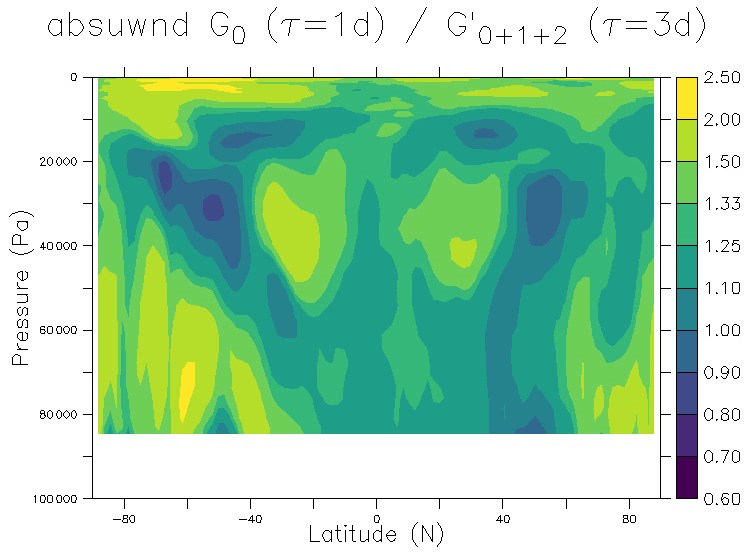
Figure 7 Ratio of the zonal mean absolute zonal wind bias correction increments G (annual mean for 1981 to 2000) between those used for C₀ (noted G₀, with τ=1 d, as in the rest of this paper) and those used in a supplementary test simulation with twice iterated bias corrections and τ=3 d (noted $G_{\mathrm{0}+\mathrm{1}+\mathrm{2}}^{\prime }$). Values between 100 000 and 85 000 Pa are not shown in the lower part of the figure. They are not relevant as, by construction, the absolute values of the increments vanish at these altitudes (see Fig. 1).

4.3 Over-correction: Out-of-sample vs. in-sample evaluation

An obvious risk of iterative bias correction procedures is over-correction of model biases, leading to degraded or physically less meaningful results when the model is applied outside of the calibration period. To detect possible signs of over-correction, the difference of the global mean RMSE reduction in corrected simulations between the calibration period (1981–2000, “in-sample”) and the normal evaluation period (2001–2020, “out of sample”) is displayed in Fig. 8 for mean annual zonal and meridional wind speed at different levels in the atmosphere. The idea is that if, as the number of iterations increases, the performance during the out-of-sample period (2001–2020) is systematically degrading compared to the performance during the in-sample period (1981–2000), then this means that the real added value of additional iterations is decreasing. As Fig. 8 suggests, this seems to be the case at least after three iterations. In that case, while for several variables the in-sample score still continues to increase, the out-of-sample score starts to decrease. This is particularly the case for variables which have low overall bias reduction scores, for example the 700 hPa meridional wind. The difference between the evolution of the in-sample and the out-of-sample scores is weaker for variables which have strong bias correction scores, such as the 200 hPa zonal wind.

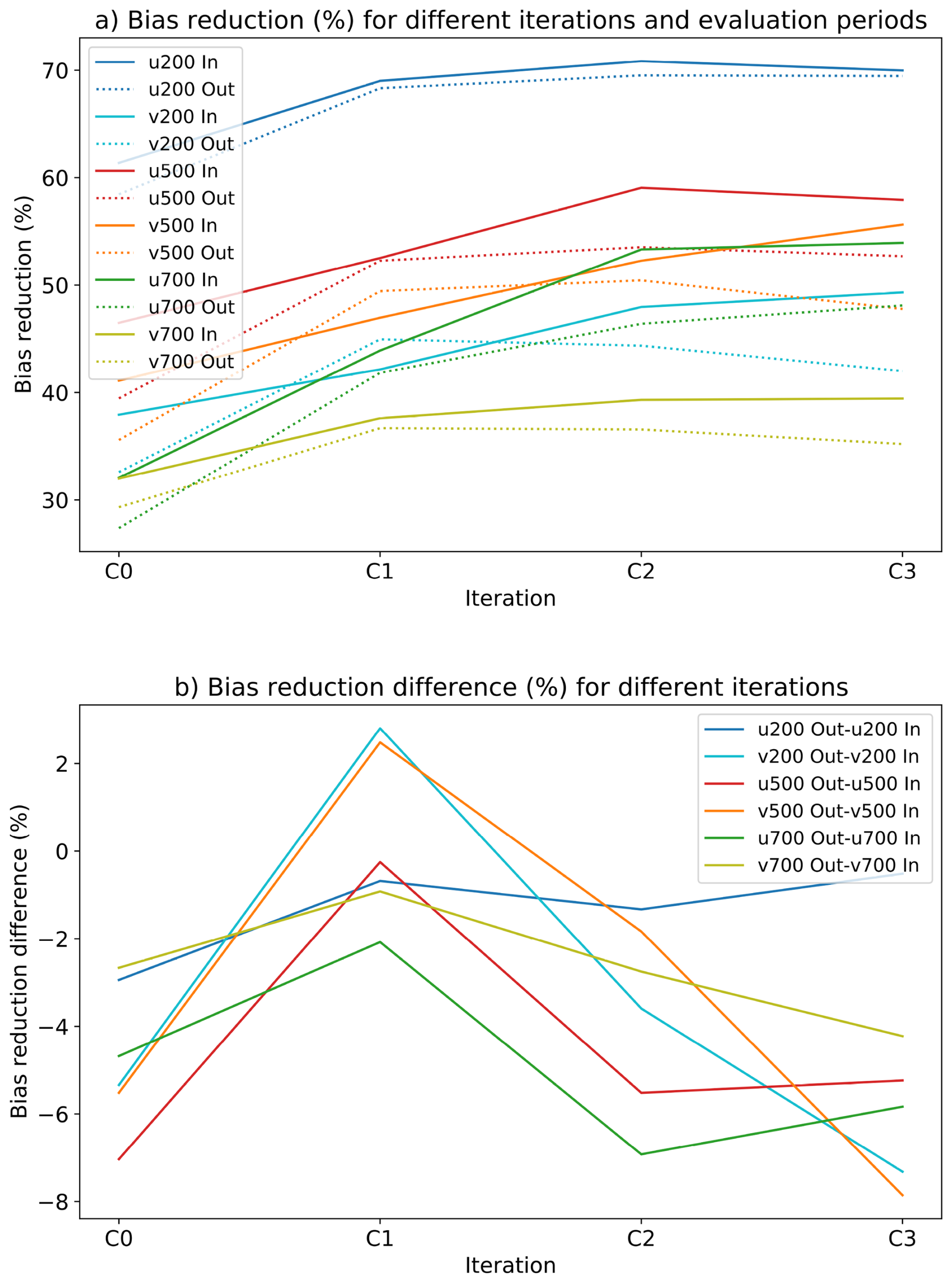
Figure 8 Comparison of bias reduction compared to the uncorrected control simulation M (in %) between different evaluation periods. (a) Bias reduction for in-sample and out-of-sample periods, for each variable; (b) Difference between in-sample and out-of-sample periods, for a given variable. As the model is nudged during the years 1981–2000, the period 1981–2020 corresponds to in-sample evaluation (noted “In”), while 2001–2020 corresponds to out-of-sample evaluation (noted “Out”).

It therefore seems that after about three iterations of the bias-correction method, the performance during the out-of-sample period is degrading compared to the performance during the in-sample period, in particular for variables for which still some potential for correction is left. As a precaution, we interpret this as a sign of over-correction, suggesting that two iterations of the bias correction method should be the maximum number in practical applications.

It is possible, however, that there is some interference between possible over-correction and the fact that the study period, 1981–2020, is a period of strong climatic change. Although it has been shown before that nudging-based ERBC remains valid under strong climate change (Krinner et al., 2020), part of the performance over the 2001–2020 period might therefore be influenced by the climate change signal. One could, as an additional test, use 2001–2020 as the ERBC calibration period and 1981–2000 for validation, or use pair years between 1981 and 2020 for the ERBC calibration and odd years of the same period for out-of-sample testing. However, the main motivation for our use of various ERBC approaches is to eventually use it in climate change simulations. In that sense, evaluating the effect of the bias corrections in a climate that is warmer than the calibration period, but still known, is a relevant test for the intended use of the ERBC approach.

4.4 Persistence and attenuation of bias patterns

We have shown that globally the mean biases are progressively reduced during the iteration of the bias correction, at least until the point when over-correction starts to occur. However, it is clear that the overall structure of the bias patterns is robust, as can be seen very clearly for example in Fig. 3. This is not surprising, as climate model bias patterns are quite persistent even under strong climate change (Krinner and Flanner, 2018; Krinner et al., 2020).

What is noteworthy nevertheless is that the strength of attenuation of mean biases is to some degree spatially variable. For example, while Fig. 3 shows a steady decrease of the annual mean 500 hPa zonal wind mean bias in the Southern Indian Ocean with increasing number of iterations of the bias correction, the corresponding bias pattern over Western Europe (positive over the Mediterranean and negative over North-western Europe) quickly stabilises, and is even amplified in simulations C₂ and C₃ relative to C₀ and C₁. Similarly, while biases continue to decrease over the North Pacific, they already start to re-increase in simulation C₂ over the South Pacific. The reasons for regional persistence of biases are not clear, and they probably are region-specific. It is for example possible that these regionally varying behaviours are linked to region-specific factors such as topography, or that they are caused by teleconnection patterns in interaction with error compensation (in the sense that in two regions linked by teleconnection mechanisms, well correcting an error in one region might unmask errors in the other region).

As a consequence, iterating the bias correction method might allow regional climate modelers to dispose of much improved atmospheric boundary conditions for the RCM in one specific region, but not in another. A detailed analysis for the reasons of bias persistence in specific regions is beyond the scope of this paper, and these reasons can depend on various factors, possibly including resolution, and are probably model-dependent. Regional bias persistence in different variations of ERBC is analysed in more detail in Champouillon et al. (2026).

4.5 Simple multiplication of correction increments

As we have shown here (see for example Fig. 3), the geographical patterns of the mean model biases are somewhat independent of the number of iterations, and the mean absolute bias correction increments increase with the number of iterations (see Fig. 2). This might suggest that as a first simple approach one could try to use a multiple of the bias correction terms obtained during the first nudging (that is, those applied in C₀) as a surrogate for the more costly iteration procedure. We have carried out a simple test in which the correction terms of C₀ are amplified by 50 %; otherwise this simulation (referred to as C${}_{\mathrm{0},\times \mathrm{1.5}}$ in the following) is identical to C₀. The analysis of C${}_{\mathrm{0},\times \mathrm{1.5}}$ shows that the bias correction is less efficient than in C₀. For example, with respect to ERA5, the annual mean global RMSE of the 500 hPa zonal and meridional wind components is 7.5 % (u₅₀₀) and 15.6 % (v₅₀₀) higher in C${}_{\mathrm{0},\times \mathrm{1.5}}$ than in C₀. However we note that C${}_{\mathrm{0},\times \mathrm{1.5}}$ still shows a substantial improvement compared to the uncorrected model run M.

It is fairly easy to understand why the model performance degrades between C₀ and C${}_{\mathrm{0},\times \mathrm{1.5}}$. As one can see in Fig. 2, although the amplitude of the correction terms does increase essentially everywhere for higher iterations of the correction procedure, the ratio of the correction terms between different phases of the iteration procedure is not uniform – it clearly has a spatial structure. A simple overall increase of the initial correction terms, although modest in our test, does not reproduce this spatial structure.

5 Conclusions

This work has shown that iterating the “classical” empirical run-time bias correction method described by Guldberg et al. (2005) once or twice (as in our simulations C₁ and C₂, respectively) substantially reduces the mean bias of the bias-corrected variables compared to simulations in which the bias correction procedure is not iterated. However, the representation of atmospheric circulation variability on interannual and shorter timescales is not always improved in simulations with iterated bias corrections. Signs of over-correction appear after about three iterations of the bias correction procedure.

All in all, the method described is easy to implement, adds substantial value and does not represent a very high additional cost compared to the non-iterated procedure.

Several other variants or further developments of run-time bias corrections have been proposed, such as a method based on direct compensation of diagnosed model biases (“CABCOR”: Scinocca and Kharin, 2024) or inference of bias-correction terms using machine learning (Watt-Meyer et al., 2021). We have implemented the CABCOR method in LMDZ and found it to yield very good results, in many respects equivalent to the iterative method presented here. We have also developed a method of state-dependent bias corrections based on the simulated instantaneous synoptic situation (as expressed in the regional 500 hPa geopotential field) as a variant of the “classical” nudging-based ERBC. These approaches are evaluated in the context of LMDZ and without temperature correction by Champouillon et al. (2026). In addition, we are currently implementing machine-learning-based inference of state-dependent ERBC in LMDZ, following Watt-Meyer et al. (2021).

More generally, because ERBC implementation choices and thus the corresponding results are at least partly model-dependent, it would be interesting to see the effect of iterative ERBC in other models, possibly in the framework of a coordinated multi-model intercomparison of various ERBC methods.