AgPaDS v1.0: a GPU-accelerated interactive Lagrangian atmospheric transport model with 3-D in situ visualization for simulating windborne dispersal of crop pathogens

Lagrangian models are widely adopted to study atmospheric transport processes, with applications in various domains, including the investigation of windborne crop diseases and epidemic risks in agriculture. Widely used Atmospheric Transport Modelling frameworks (ATMs) do not exploit the potential for performance gains and advanced computer graphics that Graphical Processing Units (GPUs) provide, and they impose limitations regarding customization for domain-specific applications in crop epidemiology and agrometeorology. The objective of this study is to contribute to addressing these gaps by developing and testing a new simulation model. We introduce AgPaDS, the Agricultural Pest and Disease Simulator, a GPU-accelerated stochastic Lagrangian model with an option for advanced interactive 3-D in-situ visualization of global-scale atmospheric transport simulations. The tool was developed with two main goals: (i) accelerate compute times through an efficient GPU implementation that enables exploratory visual analyses by means of interactive simulation setup in a graphical user interface with embedded 3-D in situ visualization; (ii) build a new atmospheric transport model dedicated to applications in crop epidemiology with model components not available in widely used ATMs and with flexibility for future domain-specific customizations. It is based on an optimized massively parallelized CUDA C$++$ and OpenGL implementation. We report on model formulation, technical implementation and testing, including a systematic comparison with HYSPLIT, one of the most widely used ATMs, and a case-evaluation with in-situ visualization of complex 3-D dynamics of simulated crop pathogen transport during the hurricane that has likely transmitted soybean rust into the USA in 2004. We show that AgPaDS produces atmospheric transport quantities broadly consistent with HYSPLIT across a set of test cases whilst providing substantial speedups for simulations with very large particle numbers (up to three orders of magnitude). The model can simulate the release of millions of Lagrangian particles from heterogeneous crop landscapes on global scales with live 3-D visualization of simulated windborne dispersal of crop pathogens. A set of supplementary videos illustrates interactive and in situ 3-D visualization methods. Examples of future use-cases include (i) exploratory 3-D visual analyses of atmospheric transport simulations, including interactions between meteorological and biological processes; (ii) assessment of global airborne connectivity of agricultural landscapes; (iii) efficient representation of wind dispersal in crop disease forecasting systems.

1 Introduction

Trillions of fungal spores, bacteria and insects form largely invisible flows of biological matter in the atmosphere (Aylor, 2017; Brown and Hovmøller, 2002; Hu et al., 2016; Huang et al., 2024; Isard and Gage, 2000; Morris et al., 2025; Schmale and Ross, 2015). Despite their significance for earth system dynamics (e.g., nuclei for cloud formation), ecology, agriculture, and health, these bioflows and their spatiotemporal dynamics are still poorly understood in exact quantitative terms. Typical numbers of airborne fungal spores and bacteria in the near-surface air that we breath in every few seconds are in the order of 10⁴ m⁻³ (Fröhlich-Nowoisky et al., 2016) and typical numbers of pathogenic fungal spores released during rust epidemics are in the order of 10¹⁰–10${}^{\mathrm{12}}{\mathrm{ha}}^{-\mathrm{1}}{\mathrm{d}}^{-\mathrm{1}}$ (Aylor, 1986; Isard et al., 2007; International Maize and Wheat Improvement Center, 1992). Several of the most devastating crop diseases and insect pests can be transported by winds over extremely long distances; they cross landscapes, regions, countries and even entire continents (e.g., soybean rust, wheat yellow rust, desert locust; Aylor, 2017; Meyer et al., 2017b; Brown and Hovmøller, 2002). The global burden of crop pathogens and pests – windborne and others – on staple food crops is estimated at 17 %–30 % yield loss (Savary et al., 2019), highlighting their relevance for food security. Research on windborne transmission of crop pathogens and insect pests on landscape to global scales is limited in large parts by gaps in available empirical data, but also because new computational techniques are required for examining, understanding and revealing the complex interplay of meteorological and biological processes governing the rich dynamics of biological flows in the atmosphere, for showing and communicating their importance, and for translating findings to actions for improving surveillance, control and early warning in agriculture (Aylor, 2017; Gilligan, 2024; Ristaino et al., 2021; Schmale and Ross, 2015).

Since the early empirical confirmation of windborne crop pathogen transmission obtained in 1930 via sampling of rust spores at an altitude of approximately 4.5 km from a plane circling above an epidemic outbreak of wheat rust, and initial mathematical modelling approaches of pathogen dispersal distances, based on typical settling velocities of fungal spores and mean horizontal wind speeds (Gregory, 1945), substantial improvements in understanding and capacity to quantify and forecast atmospheric transport of crop pathogens and insect pests have been achieved by simulation approaches, enabled by advanced computing hardware, numerical weather prediction, Atmospheric Transport Modelling frameworks (ATMs), and progress in biological modelling (Aylor, 2017; Schmale and Ross, 2015). A common methodological approach in previous work is the use of broadly applicable Lagrangian ATMs, such as the Hybrid Single-Particle Lagrangian Integrated Trajectory Model (HYSPLIT; Stein et al., 2015) or the Numerical Atmospheric Dispersion Modelling Environment (NAME; Jones et al., 2007), with input parameters configured for applications in crop epidemiology (Bradshaw et al., 2022; Burgin et al., 2013; Chapman et al., 2012; Li et al., 2025; Meyer et al., 2017b, a; Radici et al., 2021, 2022; Retkute et al., 2024; Sadyś et al., 2014; Visser et al., 2019). Another previous Lagrangian approach is the Integrated Aerobiological Modelling System (IAMS), which has been developed for domain-specific use in crop epidemiology with focus on one specific disease, soybean rust, and the risks it poses to US agriculture (Isard et al., 2005). Lagrangian models form important components in crop disease and insect pest early warning systems (Allen-Sader et al., 2019; Burgin et al., 2010; Isard et al., 2005, 2011; National Oceanic and Atmospheric Association (NOAA) – United Nations Food and Agriculture Organisation (FAO) Desert Locust, 2026).

ATMs provide flexible and detailed parameterizations for many physical processes involved in atmospheric transport, but the options for modelling biological processes and system dynamics are limited, e.g., in the field of crop epidemiology, regarding the representation of (i) complex heterogeneous crop landscapes as sources, (ii) pathogen viability decay during atmospheric transport and (iii) feedbacks with processes on the surface, such as infection dynamics during an epidemic outbreak. From a conceptual perspective on appropriate model design, it is not directly evident what level of detail is required for modelling physical and biological processes, respectively, involved in windborne transmission of crop diseases and insect pests, as this strongly depends on the specific type of application. In many applications in crop epidemiology, the available empirical data for initializing and testing mechanistic ATMs are associated with large uncertainties, the quantitative understanding of biological processes and interactions with meteorological drivers is limited, and the implications of certain meteorological regimes for risks posed to agricultural production by windborne transmission of crop diseases are challenging to assess and predict. These circumstances emphasize the need for a flexible set of modelling tools and computational workflows that can be selected and tailored to specific application cases, including also methods for exploratory analyses, identification of new hypotheses, experimentation with new domain-specific sub-models, and advanced geospatial visualization of simulation data for improving understanding, interpretation and communication of results. Broadly applicable ATMs that have been developed over the course of the last decades are well tested and flexible for applications in various thematic domains but are based on Central Processing Unit (CPU) implementations and compute workflows involving post-processing and file input/output of simulation data for visualization. Computational workflows based on these ATMs, with input parameter configuration adapted to use-cases in crop epidemiology, have proven to be of great use, and will continue to be indispensable for continued progress. However, these impose restrictions on the flexibility for specific simulation configurations and customizations for addressing some of the current active lines of research regarding airborne transport of crop pathogens and insect pests. Specifically,

• Unknowns und uncertainties around pathogen viability decay during atmospheric transport. Previous uncertainty estimates for processes involved in atmospheric transmission of crop pathogens (Aylor, 1986, 2017), and recent large scale sensitivity analyses (Meyer et al., 2017b, a; Prank et al., 2019; Visser et al., 2019) identify pathogen viability as one of the key parameters determining atmospheric transmission risks, but existing ATMs only provide limited simplistic options for representing this process and for examining, understanding and formulating new hypothesis about the effect of meteorological drivers and weather regimes on pathogen viability during atmospheric transport.

• Computation of airborne connectivity networks. Recent work combining ATMs with complex networks approaches has provided new insights for targeting surveillance and control campaigns and revealed supportive evidence for associations between windborne connectivity of crop landscapes and genetic similarity of pathogen populations in these landscapes (Choufany et al., 2021; Gilligan, 2024; Li et al., 2025; Meyer et al., 2017b; Radici et al., 2022; Sutrave et al., 2012). Computing airborne connectivity networks requires assessing airborne transport quantities between large numbers of source and target nodes, as input for constructing the weights of edges, which poses computational challenges when running detailed ATM simulations from each source cell.

• Representing heterogeneous crop landscapes as source terms. As crop pathogens and insect pests are released from complex crop landscapes, and as small changes in initial position of atmospheric transport processes can have substantial effects on resulting transmission risks, it would be beneficial and necessary in some cases to represent details of spatial characteristics of crop landscapes in source term definitions of ATMs. For example, recent genetic analyses provide novel perspectives on likely global scale exotic incursion events of wheat yellow rust (Hovmøller et al., 2026), but whilst likely geographical regions (scales of hundreds of kilometers) of interest can be identified, the exact geographical location or extent of source and receptor regions for these first incursion events remains unknown. This poses computational challenges when using a generic ATM without an option for heterogeneous gridded source terms, as it would require defining a large set of source cells arranged to cover entire crop landscapes, which often requires dedicated large-scale HPC experiments.

• Representing large numbers of source terms. Recent international crop disease and insect pest surveillance campaigns (Global Rust Reference Center, 2026; International Center for Maize and Wheat Improvement (CIMMYT) – Rusttracker, 2026; United Nations Food and Agriculture Organisation (FAO) – Desert Locust Hub, 2026) and novel techniques for automated detection of insect pests (BAYER, AgroCloud, Digital Solutions – MagicTrap, 2026) provide new data sources that include hundreds to thousands of infection/infestation sites distributed globally that, ideally, should all be included as source terms in ATMs used for early warning systems, but this can become computationally expensive when using comprehensive ATMs and usually requires costly dedicated HPC resources, restricting the number of feasible source locations in forecasting systems (Allen-Sader et al., 2019);

• Integration of realistic wind dispersal into epidemiological models. Linking mechanistic wind dispersal models with epidemiological meta-population models has been identified as a key challenge in crop epidemiology (Cunniffe et al., 2014) and it has been shown in a recent case-study that this can improve model accuracy for predicting crop disease epidemics (Radici et al., 2024). The loose coupling of a mechanistic ATM model with separate Bayesian statistical epidemiological models in previous studies is computationally demanding and restricts the flexibility for tuning the level of detail of different model components, for representing dynamic feedbacks, and for setting up efficient parameter estimation routines (Cunniffe et al., 2014; Radici et al., 2024; Retkute et al., 2024).

• Advanced 3-D visualization for exploratory visual analyses and communication. In recent work novel 3D perspectives on complex atmospheric transport of crop pathogen and insect pests have been obtained on landscape to continental scales by using a combination of an ATM with an advanced visualization software (Meyer et al., 2023). Whilst this has proven useful in the context of early warning systems for risk communication as well as for individual detailed case-analyses, the computational workflow did not allow for exploratory visual analyses of key processes such as viability decay during atmospheric transport, because it required first running an ATM on dedicated HPC resources for a certain use-case with fixed input parameters, and then visualizing the resulting simulation data via cumbersome processing routines, prohibiting smooth workflow and exploration of patterns and trends to formulate new hypothesis.

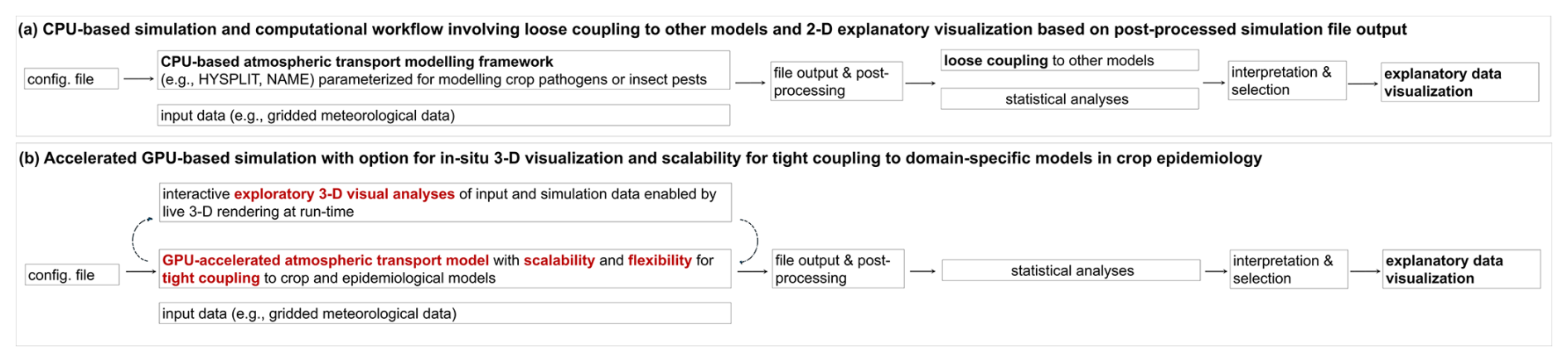
Figure 1 AgPaDS modelling approach. (a) workflow based on widely used CPU-based atmospheric modelling frameworks with post-processing of simulation data for loose coupling to other models and explanatory visualization. (b) AgPaDS modelling approach facilitating GPU-accelerated simulations with an option for exploratory visual data analyses by means of 3-D in situ visualization of simulation data and with improved scalability for tight coupling to biological models.

Recent developments in general-purpose GPU computing, computer graphics and meteorological modelling promise the potential to overcome some of the above challenges. Currently available GPUs provide immense compute power for certain tasks that can be leveraged to speed up simulations (Czarnul et al., 2020) and they provide native optimization for advanced visualization based on custom computer graphics pipelines (Rautenhaus et al., 2015). Numerical weather prediction data with increasing accuracy (Bauer et al., 2015; Govett et al., 2024) is publicly available, including consistent climatological datasets and short-term forecasting data (Hersbach et al., 2020). This in combination with recent advances in crop disease detection on field to global scales, in particular via remote sensing imagery (Yan et al., 2025) indicates the potential for notable progress in improving landscape to global scale agricultural disease and insect pest modelling in the near future. But this requires efficient computational methods capable of processing large data and detailed simulation configurations with speed and flexibility for customizations specific to crop epidemiology (Ristaino et al., 2021).

The objective of this study was to develop and test a new GPU-based Lagrangian stochastic atmospheric transport simulation tool that supports exploratory analyses by means of interactive 3-D in situ visualization and provides new model features and flexibility for domain-specific applications in crop epidemiology and agrometeorology. Figure 1 summarizes differences between previously used compute workflows in crop epidemiology based on widely used ATMs and the workflow enabled by the AgPaDS, the Agricultural Pest and Disease Simulator introduced here. In this paper, we first describe the simulation model, including goals, architecture, mechanistic simulation methods and features for interactive in situ visualization (Sect. 2), and then outline methods for model development and testing (Sect. 3). Subsequently, we report on model verification, evaluation and measurement of computational efficiency (Sect. 4) and conclude with a discussion of testing results and potential domains of use (Sect. 5).

2 Model description

This Section describes the model concept, formulation and implementation. First, modelling goals (Sect. 2.1) and model architecture (Sect. 2.2) are introduced, then a synthesis of computational implementation is given (Sect. 2.3.), followed by a summary of formal model definitions and computational aspects of parallelization and optimization for implementing the simulation model (Sect. 2.4) and the computer graphics methods for interactive 3-D in situ visualization (Sect. 2.5).

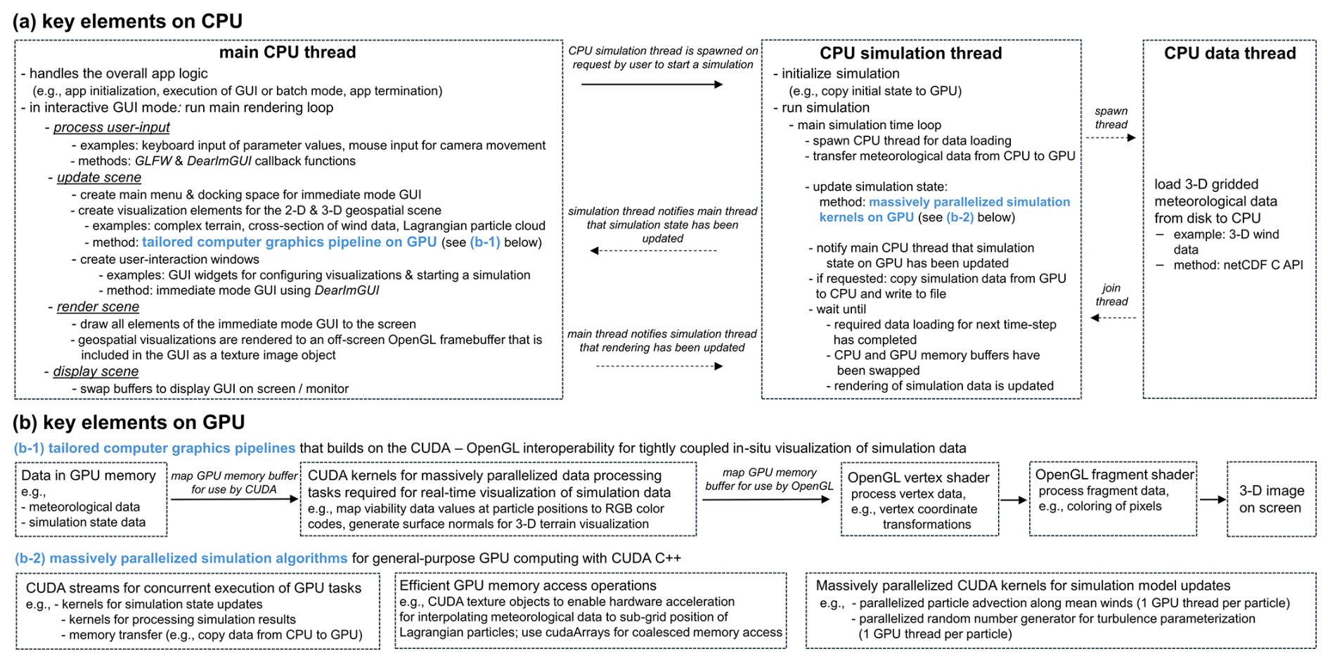
Figure 2 Conceptual summary of heterogeneous CPU-GPU implementation. (a) key elements on CPU, including tailored multi-threading for efficiency; (b) key elements on GPU, including tailored computer graphics pipelines and massively parallelized simulation algorithms.

2.1 Model goals

The simulation tool was designed with the following objectives:

• from a methodological perspective, develop a GPU-accelerated atmospheric transport model that enables, for the first time, interactive 3-D in situ visualization of stochastic Lagrangian particle simulations on global scales to obtain a tool that might complement existing ATMs by facilitating

  • a.

    exploratory 3-D visual analyses, interactive parameter sensitivity studies, visual debugging, and advanced geospatial visualization for communication purposes and teaching,

  • b.

    computational performance gains for numerical experiments that require very large numbers of Lagrangian particles, and

• from a domain-specific perspective, develop a modelling tool dedicated to simulating windborne dispersal of crop diseases and insect pests to provide custom model features not currently available in widely used ATMs that facilitate addressing open questions in crop epidemiology as part of future research, as notably

  • a.

    efficient representation of heterogeneous crop landscapes as sources,

  • b.

    efficient simulation of windborne transport from large numbers of sources, e.g. to facilitate real-time model estimates of crop disease and insect pest transmission risks from a large set of globally distributed infection sites for purposes of early warning and forecasting,

  • c.

    selection of different sub-models for viability decay during atmospheric transport,

  • d.

    interactive 3-D visual examination of the effect of meteorological factors on pathogen biology, e.g. viability decay during atmospheric transport,

  • e.

    efficient calculation of airborne connectivity of agricultural landscapes on global scales,

  • f.

    advanced 3-D geospatial visualization of windborne crop disease and insect pest transmission over crop landscapes,

  • g.

    full flexibility for future model code adaptations and extensions to allow for tailored simulation model development for, e.g., representing specific patho-systems in detailed case analyses, conducting numerical experiments tailored to new field or lab studies, tight coupling to epidemiological and crop growth models, extensions to simulate insect pest flight.

2.2 Model architecture

Simulation model inputs, main features and outputs are summarized in Fig. S1 in the Supplement. Central input for AgPaDS are gridded meteorological data as well as, for use-cases in crop epidemiology, gridded crop production and crop disease data, along with auxiliary data and parameter configurations. AgPaDS can be run in two different modes, GUI mode for exploratory visual investigations, interactive parameter sensitivity analysis and model development, and batch mode for systematic, hypothesis driven confirmatory analyses or large-scale numerical experiments and parameter sweeps. The two core model features of AgPaDS are (i) massively parallelized mechanistic simulation algorithms to model atmospheric transport, and (ii) advanced computer graphics methods that allow for interactive and in situ 3D visualization. As output in the interactive GUI mode, AgPaDS provides advanced geospatial visualizations of input and simulation data along with live calculation of basic descriptive statistics; in batch mode, two types of simulation results can be written to file: Lagrangian particle data (e.g., positions, viable pathogen material carried by particles, meteorological data at particle positions) and gridded output metrics (e.g., 2D raster data with material deposition fluxes).

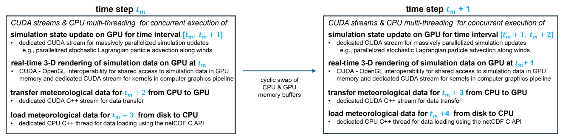
Figure 3 Time-streaming with cyclic swap of CPU & GPU memory buffers for concurrent loading of data from disk to CPU, transfer of from CPU to GPU, simulation state update and real-time rendering on GPU.

2.3 Synthesis of computational implementation

Key elements of the heterogeneous CPU-GPU workflow are summarized in Fig. 2. In short, the CPU handles overall orchestration of app and simulation logic, input data loading and rendering loop, whilst the computationally heavy tasks for simulation and visualization are massively parallelized by means of custom CUDA C$++$ and OpenGL implementations for execution on the GPU. On the CPU, the main thread coordinates overall app flow and, in GUI mode, executes the main rendering loop, whilst two separate dedicated CPU-threads are responsible for coordinating the atmospheric transport simulations and loading of meteorological data from disk. Computationally expensive tasks for simulation and for real-time 3-D visualization are executed on the GPU, using low level implementations that make efficient use of the high number (thousands) of computational cores on GPUs that can access fast shared memory and are optimized for computer graphics rendering. Whilst the overall computational bottleneck for simulation times depends on the specific model configuration, the tasks that usually require most of the computational resources are (i) loading of very large 3D meteorological input data, (ii) transfer of input data from CPU to GPU, (iii) calculation of stochastic Lagrangian atmospheric transport along winds, and (iv) computation of complex real-time interactive 3D geospatial visualization scenes. The AgPaDS modular code structure is summarized in Fig. S2 depicting an overview of main classes.

2.4 Atmospheric transport simulation model description

AgPaDS simulates key processes involved in atmospheric transport of biological matter: release from a source, atmospheric transport along winds, viability decay during transport and deposition to the surface. The spatial model domain is discretized into a regular horizontal latitude-longitude grid, with pressure as the vertical coordinate (longitudes denoted as λ, in units [degrees]; latitudes denoted as ϕ, in units [degrees]; and pressure denoted as p, in units [hPa]). To introduce the simulation model a brief conceptual summary is given in this paragraph before providing details of each process model in the Sections below. In conceptual terms, noted for application in crop epidemiology following Aylor (2017), the deposition of crop pathogen material to the surface, $D\left(\mathit{x},t;M_{\mathit{\lambda }\mathit{\varphi }\mathrm{p}}\right)$, at location, x, and time, t, in units [m ha⁻¹ d⁻¹], can be described as

$$\begin{array}{}\text{(1)}& \begin{array}{rl}& D\left(\mathit{x},t;M_{\mathit{\lambda }\mathrm{\Phi }\mathrm{p}}\right)\\ & =\underset{C\left(x,t;M_{\mathit{\lambda }\mathrm{\Phi }\mathrm{p}}\right)}{\underbrace{s_j\left({\mathit{x}}_{\mathrm{0}},t_{\mathrm{0}};M_{\mathit{\lambda }\mathrm{\Phi }}\right)\cdot T\left(\mathit{x},t;M_{\mathit{\lambda }\mathrm{\Phi }\mathrm{p}}\right)\cdot m_{\mathit{\nu }}\left(\mathit{x},t;M_{\mathit{\lambda }\mathrm{\Phi }\mathrm{p}}\right)}}\\ & \cdot {\mathit{\nu }}_{\mathrm{dep}}\left(\mathit{x},t;M_{\mathit{\lambda }\mathrm{\Phi }\mathrm{p}}\right)\end{array}\end{array}$$

where $s_j\left({\mathit{x}}_{\mathrm{0}},t_{\mathrm{0}};M_{\mathit{\lambda }\mathit{\varphi }\mathrm{p}}\right)$ represents pathogen release from source, j, at location, x₀ and time, t₀, that may depend on input data, M_λϕ, such as gridded crop production data; $T\left(\mathit{x},t;M_{\mathit{\lambda }\mathit{\varphi }\mathrm{p}}\right)$ represents a transport function that simulates atmospheric pathogen transport along winds as a function of 3-D meteorological input data, M_λϕp; and $m_{\mathrm{v}}\left(\mathit{x},t;M_{\mathit{\lambda }\mathit{\varphi }\mathrm{p}}\right)$ defines pathogen viability decay during atmospheric transport. Pathogen release, atmospheric transport and viability decay determine the pathogen material concentration in air [material/volume], denoted here as c(x,t), of which a certain part is deposited to the surface, expressed here in the form of a generic deposition function, ${\mathit{\nu }}_{\mathrm{dep}}\left(\mathit{x},t;M_{\mathit{\lambda }\mathit{\varphi }\mathrm{p}}\right)$. The above conceptual formulation is realized numerically in Lagrangian atmospheric transport models by defining a set of

$$\begin{array}{}\text{(2)}& i=\mathrm{1},\mathrm{\dots },N\end{array}$$

simulation particles that are transported along winds defined in meteorological input data. Eulerian quantities, such as material concentration per grid cell, c(x,t), are obtained as a function of the Lagrangian particle number density [number of particles/volume], $n\left(\mathit{x},t\right),$ and the material carried by each simulation particle, m_i, i.e. $c\left(\mathit{x},t\right)=m_i\cdot n\left(\mathit{x},t\right)$. In stochastic Lagrangian dispersion simulations, this is expressed in terms of the probability density function, p(x,t), for the random particle position as,

$$\begin{array}{}\text{(3)}& c\left(\mathit{x},t\right)=m_i\cdot n\left(\mathit{x},t\right)=m_i\cdot N\cdot p\left(\mathit{x},t\right)\end{array}$$

and it can be shown that the numerical solution of the set of stochastic differential equations governing the ensemble of N simulation particles provides an accurate approximation of turbulent atmospheric transport (Lin, 2013).

In AgPaDS two types of Lagrangian atmospheric transport simulations are available: mean trajectories and stochastic particle dispersion, the details of which are described in subsequent sections.

2.4.1 Spatiotemporal domain and grid

AgPaDS is designed for global, regional or landscape-scale model domains. The core 3-D spatial grid (extent and resolution) for atmospheric transport simulations is defined as the grid of the meteorological input data. AgPaDS can further represent a separate 2-D spatial grid defined by the crop input data, and it allows for user-defined grid definition for certain output analytics. The model operates in discrete time, with two characteristic time-steps: one defined by the resolution of the meteorological input data (e.g., hourly as given in ECMWF's ERA5 – the fifth generation of the European Centre for Medium-Range Weather Forecasts Reanalysis Data, as used here) and one defined as input parameter for the Lagrangian particle integration (e.g., 5 min, as used here for many test cases). The model can be used for different temporal extents, from climatological assessments to short-term forecasting, constrained by the available meteorological input data.

Computational implementation and parallelization: (i) a key computational bottleneck for enabling long simulation time extents is the processing of meteorological input data. To address this, we use a fast SSD drive and implement an efficient time-streaming algorithm that requires loading only 3 time-steps of meteorological data at any time in the simulation, avoiding the need for costly pre-loading of all meteorological data, and making use of dedicated CPU multi-threading and CUDA streams for concurrent loading of data from disk to CPU, transfer of data from CPU to GPU, and simulation state update and live 3-D rendering on the GPU (Fig. 3); (ii) a key computational bottleneck for enabling global scale and high resolution limited domain simulations are processing times associated with compute operations on large numbers of grid-cells. To address this, various grid-based calculations are accelerated by means of massively parallelized implementations that assign one GPU CUDA thread per computational grid-cell, allowing for concurrent execution of compute tasks for thousands of grid-cells.

2.4.2 Terrain

The model constructs a global 3-D terrain based on ECMWF's (European Centre for Medium-Range Weather Forecasts) ERA5 data on geopotential at the surface to approximate orography.

Computational implementation and parallelization: interactive 3-D visualization of the complex global 3-D terrain is enabled by custom CUDA kernels for massively parallelized computation of terrain vertex data, such as surface normals, combined with custom OpenGL rendering calls that, e.g., allow for interactive setting of basic lighting to improve spatial perception.

2.4.3 Input data

Gridded meteorological data are required as key input for mechanistic simulation of atmospheric transport processes. Specifically, a set of global 2-D and 3-D meteorological data grids are used to construct a digital representation of the atmosphere, with input data grid specifics defining the internal computational grid. As meteorological input data here we use ECMWF's hourly surface and pressure level ERA5 data (Hersbach et al., 2020). The data has an approximate spatial resolution of 0.25 × 0.25 decimal degrees. A total of 27 pressure levels (all available levels up to 100 hPa) are used to cover altitudes from the surface up to approximately 15 km a.s.l. Initial tests with other types of meteorological data (UKMO UM, ICON) have been conducted but are not included here. A second central input are crop production data. Global gridded crop data (International Food Policy Research Institute (IFPRI), 2024) for 46 different crops can be loaded into AgPaDS, as optional input for defining heterogeneous gridded crop source areas or as a layer in the interactive visualization scene. Initial trials with loading other types of gridded crop data that include seasonal crop phenology approximations were conducted but are not yet included here. Crop disease or insect pest surveillance data is loaded in tabular format and can be included in interactive 3D visualizations or used to define source locations for Lagrangian particle simulations. Auxiliary data, such as administrative boundaries, can be loaded optionally, e.g., for providing context in 3D visualizations or for custom analytics.

The specifically required 2-D and 3-D input data variables depend on the use-case and choice of model configuration. For example, (i) the spatiotemporal dynamics of global temperature variations in ERA5 could be examined interactively in 3-D over a certain crop landscape of choice as part of an exploratory visual analyses of input data that only requires ERA5 temperature as input; (ii) the minimum required input data for mean trajectory calculations are the three wind data fields on pressure levels (longitudinal, latitudinal and vertical wind velocity fields) and surface pressure; whilst (iii) for more detailed stochastic Lagrangian particle dispersion simulations from gridded crop landscapes as a source, and including a parameterization of non-resolved turbulent winds, viability decay and deposition processes, a set of additional input data are required, such as, gridded crop production data, boundary layer height, friction velocity, UV radiation, temperature and relative humidity.

Computational implementation and parallelization: (i) Meteorological data is loaded into AgPaDS in the form of a generic netCDF file format so that, in principle, different types of meteorological data can be processed as input in future applications with appropriate pre-processing. Data conversion scripts for ERA5 are provided in the Supplement; (ii) AgPaDS requires handling of large input data. For example, one hourly time-step of global 3-D meteorological data for one meteorological variable, e.g. temperature, on 27 pressure levels, contains approximately 28 million data entries, amounting to approximately 110 MB file size in the single precision floating point netCDF format required for AgPaDS. This corresponds to around 8 GB of meteorological input data with around 2 billion data points that need to be processed efficiently when conducting one day of global scale atmospheric mean trajectory simulations that require three wind data fields as 3-D input data; (iii) for efficient loading of meteorological data, CPU-multi-threading is used with a dedicated CPU thread that has the sole task to load meteorological data from disk using the netCDF C API, whilst other parts of the simulation are executed concurrently; (iv) gridded global crop input data with a spatial grid resolution of 0.083 [decimal degrees] is used, requiring the processing of approximately 9.3 million grid-cells with crop production data, of which, for example in the case of wheat crop, approximately 250 000 grid cells contain non-zero crop production values, which are all considered for defining gridded heterogeneous crop landscape as source terms.

2.4.4 Source term

The following types of source geometries can be defined in AgPaDS: point sources based on input data providing geographical coordinates (e.g., crop disease surveillance data with coordinates of individual infected fields); rectangular sources defined by center coordinates and latitudinal, longitudinal, and vertical extent; and heterogeneous gridded crop area sources, defined by crop input data clipped to a user-defined rectangular geographical extent. Both instantaneous and continuous particle release during a user-defined release time-window is supported.

The initial position of Lagrangian simulation particles, ${\mathit{x}}_i^{\mathrm{0}}$ is defined at the location of the source. For the rectangular and gridded source types, Lagrangian particles are randomly distributed inside the source area. The total material, M, that is released per source is uniformly distributed to all simulation particles per source,

$$\begin{array}{}\text{(4)}& m_i^{\mathrm{o}}=M/N.\end{array}$$

In line with common approaches in other ATMs (see e.g. Draxler, 1999; Jones et al., 2007), the material carried by simulation particles is independent of the actual physical mass of particles and instead represents a user-defined simulation parameter that serves to represent a transport quantity of choice, in the case of crop epidemiology, a common choice is the approximate pathogen load, expressed as an order of magnitude estimate of the number of viable fungal spores released during an epidemic outbreak in a certain geographical area.

Simulation parameters, computational implementation and parallelization: (i) Table S1 summarizes key user-defined simulation parameters to configure the source term; (ii) the custom optimization for extremely high numbers of Lagrangian particles implemented in AgPaDS (see below) provides as one key advantage the capacity for flexible definition of very large numbers of individual source terms and for the definition of heterogeneous crop landscapes as gridded sources. For example, AgPaDS can handle hundreds to thousands of individual sources in full stochastic Lagrangian dispersion mode and it can simulate heterogeneous gridded sources with hundreds of thousands of source grid cells in a cheaper trajectory mode with reduced numbers of Lagrangian trajectories per source grid cell; (iii) for efficient computation of non-instantaneous release of tens of millions of simulation particles from gridded crop area sources over an extended release time interval all required simulation particles are initialized at random positions inside the source area once during initialization on the CPU before the start of the main simulation loop, copied to the GPU and then activated and updated iteratively on the GPU as part of simulation updates during the main time loop.

2.4.5 Atmospheric transport

The atmospheric transport of Lagrangian particles, i, with position, x_i(t) defined in lat-lon-pressure space,

$$\begin{array}{}\text{(5)}& {\mathit{x}}_i\left(t\right)=\left(\mathit{\lambda }\left[\mathit{°}\right],\mathit{\varphi }\left[\mathit{°}\right],p\left[\mathrm{hPa}\right]\right)\end{array}$$

is modelled as a continuous stochastic variable, resolved to sub-grid scales relative to the spatial grid defined by the meteorological input data and with much higher temporal resolution than the meteorological input data. Particle motion in air is computed as

$$\begin{array}{}\text{(6)}& \begin{array}{rl}{\displaystyle \frac{\mathrm{d}{\mathit{x}}_i}{\mathrm{d}t}}& ={\mathit{v}}_i\left({\mathit{x}}_i;M_{\mathit{\lambda }\mathit{\varphi }\mathrm{p}}\right)={\stackrel{\mathrm{‾}}{\mathit{v}}}_{\mathrm{wind}}\left({\mathit{x}}_i\left(t\right);M_{\mathit{\lambda }\mathit{\varphi }\mathrm{p}}\right)\\ & +{\mathit{v}}_{\mathrm{stoch}}\left({\mathit{x}}_i\left(t\right);M_{\mathit{\lambda }\mathit{\varphi }\mathrm{p}}\right)+{\mathit{v}}_{\mathrm{sed}}\left({\mathit{x}}_i\left(t\right);M_{\mathit{\lambda }\mathit{\varphi }\mathrm{p}}\right),\end{array}\end{array}$$

with ${\stackrel{\mathrm{‾}}{\mathit{v}}}_{\mathrm{wind}}$ denoting advection along mean winds given in the meteorological input data, v_stoch denoting stochastic particle dispersion to parameterize non-resolved winds on shorter scales than the meteorological input, and v_sed denoting gravitational settling.

To model particle movement along winds, ${\stackrel{\mathrm{‾}}{\mathit{v}}}_{\mathrm{wind}}\left({\mathit{x}}_i\left(t\right);M_{\mathit{\lambda }\mathit{\varphi }\mathrm{p}}\right)$, the meteorological input data is interpolated in space and time to the sub-grid (relative to meteorology) location and time, x_i(t), of particle, i. As wind data in ERA5 are given in metric units, ${\mathit{v}}_{\mathrm{wind}}=\left(u\right[\mathrm{m}{\mathrm{s}}^{-\mathrm{1}}],v[\mathrm{m}{\mathrm{s}}^{-\mathrm{1}}],\mathit{\omega }[\mathrm{Pa}{\mathrm{s}}^{-\mathrm{1}}\left]\right)$, the following unit conversions are applied for particle simulations in (latitude-longitude-pressure) space: $u\left[\mathit{°}{\mathrm{s}}^{-\mathrm{1}}\right]=u\left[\mathrm{m}{\mathrm{s}}^{-\mathrm{1}}\right]/\left(L_{\mathit{\varphi }}\left[\mathrm{m}{\mathit{°}}^{-\mathrm{1}}\right]/\cos \left(\mathit{\varphi }\frac{\mathit{\pi }}{\mathrm{180}}\right)\right)$, $v\left[\mathit{°}{\mathrm{s}}^{-\mathrm{1}}\right]=v$ $\left[\mathrm{m}{\mathrm{s}}^{-\mathrm{1}}\right]/L_{\mathit{\varphi }}$ [m°−1], ω $\left[\mathrm{hPa}{\mathrm{s}}^{-\mathrm{1}}\right]=\mathit{\omega }$ $\left[\mathrm{Pa}{\mathrm{s}}^{-\mathrm{1}}\right]/\mathrm{100}$.

Following the atmospheric dispersion modelling framework NAME (Jones, 2025) the effect of non-resolved winds on Lagrangian particle simulations is parameterized using a Markov type stochastic model with two terms to mimic different scales of non-resolved winds, turbulence due to small scale eddies and mesoscale motion on scales between turbulent eddies and resolved meteorological data,

$$\begin{array}{}\text{(7)}& \begin{array}{rl}{\mathit{v}}_{\mathrm{stoch}}\left({\mathit{x}}_i\left(t\right)\right)& ={\mathit{v}}_{\mathrm{meso}.}\left({\mathit{x}}_i\left(t\right)\right)+{\mathit{v}}_{\mathrm{turb}.}\left({\mathit{x}}_i\left(t\right)\right)\\ & =\mathit{\epsilon }\sqrt{\mathrm{2}{\mathit{K}}_{\mathrm{m}}t}+\mathit{\eta }\sqrt{\mathrm{2}{\mathit{K}}_{t}t}\end{array}\end{array}$$

where, ε and η denote Gaussian white noise, i.e. normally distributed random variables with mean zero. The magnitude of stochastic displacements, which tunes the extent of atmospheric dispersion of particle plumes in air, is computed as

$$\begin{array}{}\text{(8)}& {\displaystyle }{\mathit{K}}_{\mathrm{t}}=({\mathit{\sigma }}_{\mathrm{h}}^{\mathrm{2}}\cdot {\mathit{\tau }}_{\mathrm{h}},{\mathit{\sigma }}_{\mathrm{h}}^{\mathrm{2}}\cdot {\mathit{\tau }}_{\mathrm{h}},{\mathit{\sigma }}_{\mathrm{v}}^{\mathrm{2}}\cdot {\mathit{\tau }}_{\mathrm{v}}),\text{(9)}& {\displaystyle }{\mathit{K}}_{\mathrm{m}}=({\stackrel{\mathrm{‾}}{\mathit{\sigma }}}_{\mathrm{h}}^{\mathrm{2}}\cdot {\stackrel{\mathrm{‾}}{\mathit{\tau }}}_{\mathrm{h}},{\stackrel{\mathrm{‾}}{\mathit{\sigma }}}_{\mathrm{h}}^{\mathrm{2}}\cdot {\stackrel{\mathrm{‾}}{\mathit{\tau }}}_{\mathrm{h}},{\stackrel{\mathrm{‾}}{\mathit{\sigma }}}_{\mathrm{v}}^{\mathrm{2}}\cdot {\stackrel{\mathrm{‾}}{\mathit{\tau }}}_{\mathrm{v}}),\end{array}$$

where ${\mathit{\sigma }}_{\mathrm{h}}^{\mathrm{2}}$ and ${\mathit{\sigma }}_{\mathrm{v}}^{\mathrm{2}}$ are the variances of horizontal and vertical wind speed distributions, respectively, and τ_h and τ_v are the horizontal and vertical Lagrangian timescales (i.e., the times for which turbulent fluctuations remain correlated along the path of individual particles). For non-resolved mesoscale motion, the standard deviations and Lagrangian timescales are assumed to be constant, with values taken from the NAME parameterization for hourly meteorological data (${\stackrel{\mathrm{‾}}{\mathit{\sigma }}}_{\mathrm{v},\mathrm{h}}=\mathrm{0.7}$ m s⁻¹; ${\stackrel{\mathrm{‾}}{\mathit{\tau }}}_{\mathrm{h},\mathrm{v}}=$ 8000 s) (Jones, 2025). For small-scale turbulence, the magnitude of atmospheric dispersion depends on the position of Lagrangian particles relative to the atmospheric boundary layer. Above the boundary layer, ${\mathit{\sigma }}_{\mathrm{h},\mathrm{v}}^{\mathrm{2}}$ and τ_h,v are assumed to be constant, with values defined by free troposphere values used in NAME (σ_h=0.25 m s${}^{-\mathrm{1}}{\mathit{\sigma }}_{\mathrm{v}}=\mathrm{0.1}$ m s⁻¹; τ_h=300 s; τ_v=100 s) (Jones, 2025). Inside the boundary layer the velocity variances and Lagrangian time-scales are computed as a function of planetary boundary layer height (h_b), friction velocity (v^*), and atmospheric stability (L; Monin-Obhukov length), along with constants and particle height, with definitions adapted from the turbulence parameterization in NAME (Jones, 2025). The value of atmospheric diffusivities inside the mixing layer are bound numerically from below by the constant free troposphere values and bound from above by the numerical stability criterion that total particle displacement per timestep cannot exceed the extent of one grid-cell of meteorological data.

Gravitational settling, v_sed(x_i(t);M_λϕp) is simulated following standard approaches also used in Hoffmann et al. (20212), as a function of particle diameter (r), particle density (ρ_i), density of air (ρ_air), dynamic viscosity of air (η), gravitational constant (g), and the Cunningham slip factor (C_s), as

$$\begin{array}{}\text{(10)}& {\mathit{v}}_{\mathrm{sed}}={\displaystyle \frac{C_{\mathrm{s}}\mathrm{2}{r}^{\mathrm{2}}g({\mathit{\rho }}_i-{\mathit{\rho }}_{\mathrm{air}})}{\mathrm{9}\mathit{\eta }}}\end{array}$$

By tuning input parameter configurations, the AgPaDS user can choose different schemes for simulating atmospheric transport. For example, in the simplest case, both the stochastic term and the settling term can be turned off entirely; in this case, v_stoch=0 and v_sed=0, the standard mean trajectory model is recovered, and air-parcels are advected deterministically along resolved winds in meteorological input data. In more detailed cases, Lagrangian particles might be simulated as bio-aerosols with finite mass that are subject to gravitational settling and stochastic movements that approximate non-resolved winds, carrying a user-defined pathogen material load that can be deposited to the surface.

Simulation parameters, computational implementation and parallelization: (i) Table S1 summarizes the key user-defined simulation parameters for the transport model components; (ii) the equation of motion for Lagrangian particles is solved numerically by means of an Euler forward scheme, i.e. ${\mathit{x}}_i\left(t+\mathrm{\Delta }t\right)={\mathit{x}}_i\left(t\right)+\mathrm{\Delta }t\cdot {\mathit{v}}_i(x,t)$, where the particle integration time-step, Δt, is a user-defined configuration parameter that needs be set relative to the (longer) time-step of the meteorological input data. For all simulations here the meteorological input data has an hourly resolution and a particle integration time step of Δt=5 [min] was used; (iii) the update of particle positions is fully executed on the GPU, using an optimized massively parallelized implementation with the following key specifics: (a) assign one GPU CUDA thread per Lagrangian simulation particle to allow for concurrent numerical integration thousands of particle trajectories (adapted from Green, 2008), (b) use a CUDA based random number generator on the GPU to ensure independent random displacements for all individual particles whilst speeding up costly random number generation for stochastic simulations with large particle numbers (Green, 2008; Januszewski and Kostur, 2010) and (b) load meteorological data into GPU texture memory objects that allow for efficient caching and hardware interpolation of meteorological data from grid-points to sub-grid particle positions in one memory read operation to reduce memory load times of CUDA kernels.

2.4.6 Viability decay during atmospheric transport

Four different pathogen viability sub-models with different data requirements and levels of complexity are included to provide flexibility for modelling this process, which is known to be of key importance in crop epidemiology:

in the simplest case, pathogens are either assumed to be viable or not viable,

$$\begin{array}{}\text{(11)}& m_i^{\mathrm{c}}\left(t\right)=\left\{\begin{array}{l}\mathrm{1},t<t_{\max }\\ \mathrm{0},t\ge t_{\max }\end{array}\right.\end{array}$$

where, t_max, denotes the maximum lifetime of pathogens which can be defined as an input parameter, to set the time after which simulation particles are taken out of simulation in the purely time-dependent sub-model, the decrease of pathogen viability is modelled as an exponential decay process (Meyer et al., 2017b) with the same constant decay rate for all particles,

$$\begin{array}{}\text{(12)}& m_i^{\mathrm{d}}\left(t\right)=m_i^{\mathrm{o}}\exp (-d\cdot t)\end{array}$$

in the simple UV-dependent scheme following Isard et al. (2005), viability decay is modelled as

$$\begin{array}{}\text{(13)}& m_i^{\mathrm{UV}}({\mathit{x}}_i,t)=m_i^{\mathrm{o}}\exp (-\mathit{\kappa }\cdot D({\mathit{x}}_i,t\left)\right)\end{array}$$

based on sampling the cumulative UV dose, D(x_i,t) experienced by each simulation particle during its atmospheric transport path and using a constant critical dose parameter, κ, for computing the remaining viable fraction of pathogens in a more detailed UV-dependent scheme, as introduced in (Meyer et al., 2017a), the sensitivity of pathogens to UV radiation is not constant, as in the model above, but depends on ambient relative humidity, sampled at each timestep at the position of each simulation particle during atmospheric transport and is computed as

$$\begin{array}{}\text{(14)}& m_i^{\text{UV-RH}}({\mathit{x}}_i,t)=m_i^{\mathrm{o}}\exp (-s\left(\mathrm{RH}({\mathit{x}}_i,t)\right)\cdot D({\mathit{x}}_i,t\left)\right).\end{array}$$

Simulation parameters, computational implementation and parallelization: (i) Table S1 summarizes the key user-defined simulation parameters to configure the viability decay model component; (ii) viability decay is calculated on a particle basis, facilitating a massively parallelized computation where each CUDA thread computes the loss of material during each time-step for the simulation particle that it represents; (iii) modular implementation to facilitate straightforward adaptations of the simulation framework to include other types of viability decay models in future studies, e.g., adapted to specific pathogens, or newly available empirical data.

2.4.7 Deposition to the surface

Total deposition of particle material to the surface is computed as the sum of dry and wet deposition,

$$\begin{array}{}\text{(15)}& d^{\mathrm{tot}}=d^{\mathrm{dry}}+d^{\mathrm{wet}}\end{array}$$

where dry deposition is computed as

$$\begin{array}{}\text{(16)}& d_i^{\mathrm{dry}}\left({\mathit{x}}_i,t\right)=m_i\left({\mathit{x}}_i,t\right)\cdot \exp \left(-v_{\mathrm{dep}}\left({\mathit{x}}_i,t\right)/\mathrm{\Delta }{z}_{\mathrm{o}}\right)\end{array}$$

following the approach in Hoffmann et al. (2022), and using a dry deposition velocity parameterization, v_dep(x_i,t), to scale the portion of particle material that is deposited from particles that are located inside the lowest layer of the atmosphere, defined here with a depth Δz_o of 30 hPa to the surface.

Wet deposition is computed following the approach (Isard et al., 2005) as a function of total precipitation and a critical precipitation parameter that is set such that, a precipitation total of 25.4 mm leads to wet deposition of 63.2 % of pathogen material to the surface,

$$\begin{array}{}\text{(17)}& d_i^{\mathrm{wet}}\left({\mathit{x}}_i,t\right)=m_i\left({\mathit{x}}_i,t\right)\cdot \exp (-\mathrm{TP}({\mathit{x}}_i,t)/p_{\mathrm{crit}})\end{array}$$

Simulation parameters, computational implementation and parallelization: (i) Table S1 summarizes the key user-defined simulation parameters to configure the deposition scheme; (ii) particle deposition is computed on a particle basis to facilitate massively parallelized computation; (iii) total grid-based deposition values [material/surface area/time] are obtained by summing up the contributions of all individual particles, i, per deposition grid-cell, xy, $D_{xy}^{\mathrm{tot}}\left(t\right)={\sum }_{i\in xy}{d}_i^{\mathrm{tot}}\left(t\right)$

2.5 Graphical user interface (GUI) for interactive and in situ 3-D visualization

A set of custom computer graphics methods were developed to facilitate interactive and in situ 3-D geospatial visualization of input and simulation data via a Graphical User-Interface. The custom AgPaDS GUI includes a flexible docking space for free arrangement of user windows, e.g. a window for interactive simulation parameter configuration, a window for 2-D visualization and a window for advanced 3-D geospatial data visualization. The GUI is implemented based on the ImGUI immediate mode C$++$ library (Cornut, 2025).

Figure 4 and Movie S1 illustrate the main AgPaDS GUI, along with examples of 3-D data visualizations. Table 1 summarizes the full set of methods for exploratory 3-D visual data analyses developed here, along with a short summary of the technical implementation, examplar use-cases and a reference to a supplementary movie showing a screenshot recording of the AgPaDS GUI to illustrate the method (Movies S2–S13). Exemplar use-cases of exploratory visual analyses enabled by the visualization methods developed here include, e.g., interactively navigating a virtual camera and movable 2-D data slicing planes through a 3-D scene with global meteorological data over crop landscapes; interactively configurating the source geometry for Lagrangian particle simulations inside a 3-D scene, with interactive definition of simulation parameters, and subsequent in situ visualization of stochastic Lagrangian particles, rendered as small spheres colored according to a data variable of choice, such as, e.g., the amount of viable pathogen material carried by the simulation data or meteorological data interpolated to particle positions.

Figure 4 AgPaDS Graphical User Interface with example screenshots of 3-D interactive visualization of meteorological input data and 3-D in situ visualization of Lagrangian particle transport simulations on global scales. (a) 3-D box view (with axis: [latitude, longitude, pressure]; (b) 3-D spherical globe view; (c) crop production and disease surveillance data; (d) movable vertical data slice to sample 3-D meteorological data and interactive data prober to sample individual values; (e) wind flow visualization with coloring according to horizontal wind speed with dynamic wind trails; (f) in situ visualization of Lagrangian particle simulations with release from gridded heterogeneous crop landscapes as source; (g) in situ visualization of domain filling global Lagrangian particle simulation data with coloring according to 3-D temperature (with cold to warm depicted as blue to red) at particle positions; (h) interactive vertical transparent viewing window to inspect inner structure of Lagrangian particle clouds at run-time with particle coloring as in (g). See supplementary Movies S1–S16 for screenshot recordings demonstrating interactive data exploration and dynamic in situ visualization.

Table 1 Methods for interactive 3-D visual analyses and in-situ visualization. Movies S2–S14 are available as supplementary material (see links to individual movies in section “Video Supplement” or series here: https://av.tib.eu/series/2004, last access: 3 June 2026). Table S3 summarizes key aspects of technical implementation and potential use-cases.

To obtain the necessary computational performance for interactive rendering of complex 3-D geospatial scenes involving global ERA5 meteorological data and for rendering of stochastic Lagrangian particle simulations at run-time, AgPaDS draws heavily on the CUDA – OpenGL interoperability (NVIDIA Corporation, 2025). This direct interface between custom general purpose GPU computing with CUDA C$++$ and custom computer graphics implementations based on OpenGL allows for shared access to simulation state data on the GPU for both massively accelerated simulation compute tasks and tailored low level rendering calls. It is implemented here by means of a heterogeneous CPU-GPU approach in which the main CPU thread runs the rendering loop and communicates with a separate CPU thread that controls simulation tasks, enabling the orchestration of iterative updates to rendering and simulation state, via triggering of custom compute and rendering methods that are massively parallelized for execution on the GPU and operate on GPU memory arrays that are configured for optimized performance and re-used via an iterative cyclic update of pointers to GPU memory buffers (Fig. 3). This avoids computationally expensive data copying, file Input/Output, and pre/post-processing operations, which are required as part of standard visualization workflows. For example, in a typical workflow for explanatory visualization, Lagrangian simulation data (e.g., particle positions), would be written to file by the simulation program, followed by post-processing for data conversion, and then loading into a separate visualization software, whereas here, simulation data (e.g., the position of all Lagrangian particles) are stored in GPU memory arrays that directly are accessed by both CUDA kernels for compute tasks and OpenGL rendering calls for visualization. Another key advantage of the CUDA – OpenGL interoperability is that it enables the use of general-purpose CUDA kernels for massively parallelized processing of vertex data and texture images as required as part of the computer graphics pipeline. Compared with OpenGL vertex shader code, CUDA kernels have the advantage that they are more flexible, allowing for the integration of standard C/C$++$ routines, existing numerical libraries, and pre-built components, and, importantly, different to OpenGL, there are elaborate and well-tested GPU debugging features for CUDA kernels.

3 Methods for model development and testing

This Section summarizes the model development environment (Sect. 3.1) and methods for model verification (Sect. 3.2), model evaluation (Sect. 3.3) and measurements of computational efficiency (Sect. 3.4).

3.1 Model development environment

Model development and testing was conducted on a mobile GPU workstation with the following hardware specifications: (i) GPUs: NVIDIA RTX 4000 Ada Generation Laptop GPU dedicated to custom general-purpose and computer graphics computations (compute capability 8.9; 12 GB memory; 7242 Compute Unified Device Architecture (CUDA) cores; core clock rate 2.12 GHz; approximately 31 Teraflops theoretical single-precision floating point peak performance) and a separate Intel UHD graphics card for standard display; (ii) hard drives: 2 TB SK Hynix Solid State Drive (SSD) drive and 1 TB Samsung SSD drive; (iii) installed RAM: 64 GB; (iv) CPU: i9 13th Gen Intel with 24 CPU cores and 2.2 GH base speed. Most of the model development and testing was conducted on MS Windows with selected processing, simulation and testing tasks executed on the Linux subsystem for Windows. For general-purpose GPU computations, CUDA version 12.8 with NVIDIA driver 573.57 was used, drawing on the CUDA-OpenGL interoperability, with OpenGL version 4.6.0 used for custom computer graphics methods (NVIDIA Corporation, 2025). Core simulation code is implemented in C$++$, CUDA C$++$, and OpenGL, with pre- and post-processing routines, automated simulation configuration pipelines and testing scripts written in Python, Batch and Shell. The heterogeneous CPU-GPU development was carried out in MS Visual Studio Community Edition 2022 with integrated NVIDIA Nsight GPU extension toolkit for next-generation GPU debugging and system wide performance tracing with Nsight Systems. Python script development and testing was done in MS Visual Studio Code, version 1.106.1.

3.2 Model verification

To ensure model correctness, stability and internal consistency, the following steps and procedures were carried out: (i) design of modular code for ease of testing, maintainability and future extensions; (ii) debugging of model components using the MS Visual Studio debugger for CPU-side C$++$ code and the Next-Gen NVIDIA NSight CUDA debugger for GPU code, with the latter providing comprehensive access to GPU state and simulation data in debug mode to allow for, e.g., stepping through massively parallelized GPU code in different CUDA threads for inspecting simulation variables; (iii) implementation of custom assertions, safeguards, and optional verbose logging output to ensure, e.g., plausibility of input parameters and key state variable value ranges at runtime; (iv) automated error testing for CUDA kernel calls and OpenGL code sections; (v) use of the NVIDIA Nsight Systems tool for system-wide integrated tracing of CPU and GPU processes to inspect overall logical execution of simulation flow and timing of different computational tasks, e.g., to test the sequence and concurrency of execution of different CUDA kernels and streams and to measure plausibility of computational runtimes of different code components in different simulation configurations; (vi) custom NVIDIA NVTX ranges for timing selected parts of simulation code; (vii) the custom computer graphics methods developed here for 3-D interactive and in-situ visualization were tested by visual examination of the resulting geospatial views (e.g., data slices, particle clouds, etc.) for various different input data and simulation configurations; (viii) once the custom visualization methods were running, these were used for visual debugging and verification of simulation code, which has the advantage that the in situ visualization of simulation data at runtime facilitates flexible real-time examination of complex simulation state dynamics to assess, e.g., the plausibility of 3-D dynamics of Lagrangian particle plumes; (ix) simulation methods and consistency of in-situ visualizations, live descriptive statistics and simulation output were tested in different configurations and parameterizations by inspection of selected output data in comparison with expected value ranges and visualizations.

3.3 Model evaluation

The simulation model was evaluated in three different setups: (Sect. 3.3.1) systematic comparison of AgPaDS simulation results with results from the widely used and well tested atmospheric dispersion modelling framework HYSPLIT (Stein et al., 2015) for a set of test locations in two different simulation modes (mean trajectories and stochastic dispersion runs); (Sect. 3.3.2) comparison of individual time-backwards mean trajectories in AgPaDS and in HYSPLIT; and (Sect. 3.3.3) comparison of AgPaDS with IAMS and published empirical crop disease data for the special case of the likely transmission of soybean rust into the USA caused by hurricane Ivan (Isard et al., 2007).

3.3.1 Comparing simulated atmospheric transport data from a set of test-locations from AgPaDS and HYSPLIT

AgPaDS mean trajectory and stochastic particle dispersion simulations were tested by comparison with outputs of HYSPLIT simulations. For this, a set of Python, Shell and Batch scripts were written for automated setup, execution and analysis of a suite of AgPaDS and HYSPLIT test simulations. AgPaDS was run in batch mode and file output was compared with HYSPLIT data. HYSPLIT public version 5.3.0 for Ubuntu, obtained from National Oceanic and Atmospheric Association (NOAA) – HYSPLIT (2026), was run on the Linux subsystem for Windows on the same mobile workstation as AgPaDS.

For evaluation purposes, a set of 15 test locations was defined for simulation of atmospheric mean trajectories and stochastic particle dispersion (Table S2). The coordinates of the test-locations were selected such that key wheat crop production areas are included, providing a realistic albeit synthetic test setting. As far as possible, the same simulation input configurations were used for both HYSPLIT and AgPaDS. However, there are differences between HYSPLIT and AgPaDS, e.g., regarding vertical model grid structure and some process-specific sub-models, so that some differences in simulation results between the two models are expected. As meteorological input for all test runs, the re-analysis data, ERA5, of the European Center for Medium-Range Weather Forecast (ECMWF) was used (2D surface and 3D pressure level data; hourly temporal resolution; global regular lat-lon grid with approximately 0.25 decimal degrees spatial resolution), applying the necessary conversion from ECMWF's ERA5 to NOAA's (National Oceanic and Atmospheric Administration) ARL (Air Resources Laboratory) data for HYSPLIT runs and to a generic netCDF format for AgPaDS.

To test AgPaDS mean-trajectory calculations, 10 atmospheric mean-trajectories were computed from each release location at three different release altitudes (10, 100, 1000 m a.g.l.) and results were compared with data obtained from HYSPLIT using the same setup of sources and release altitudes. The following input configuration was used for both simulation models: ERA5 meteorological input data; source location center coordinates as given in Table S2, with 10 trajectory starting locations defined via a 0.1° offset in each direction around the central position from which 2 trajectories are released; release altitudes of 10, 100, and 1000 m a.g.l., respectively; release time chosen to coincide with wheat growing regions around the source locations; and a discrete time-step for the trajectory computations of 5 min. All input parameters are available in the configuration files for test-runs provided in the code repository.

To test AgPaDS stochastic Lagrangian particle dispersion runs, 10 000 Lagrangian particles were released at one release altitude (100 m a.g.l.) from each of the 15 test-locations, defining the material release rate per location as M= 1, and simulating turbulent atmospheric transport, viability decay and material deposition to the surface. Similar input data, source locations and release timing as for the trajectory simulations were used for the stochastic Lagrangian simulations, with additional modelling of non-resolved turbulent winds, viability decay and deposition to the surface. Whilst the same viability decay scheme was used in both HYSPLIT and AgPaDS, the specifics of available turbulence parameterization and the wet deposition scheme are different (AgPaDS model definitions given in Sect. 2; HYSPLIT default turbulence and wet deposition schemes were used (Draxler, 1999). All input parameters are available in the configuration files for test-runs provided in the code repository (see Code and data availability; Meyer et al., 2026).

For evaluating AgPaDS model results in comparison with HYSPLIT, a two-step procedure was applied. In the first step, simulation output was processed to create geographical maps of mean atmospheric trajectories, stochastic particle clouds in air and deposition plumes from both simulation models (HYSPLIT, AgPaDS), which were compared visually for all test locations to evaluate similarities and differences in qualitative characteristics. Notably, key characteristics of complex plume shapes and trajectory paths were compared, including distinctive features, main directions, and approximate spatial spread. In the second step, the following set of metrics was computed for systematic comparison of quantitative characteristics of simulation data from both simulation models.

For trajectory runs, it was evaluated how AgPaDS performs with respect to the mean trajectory distance and direction from the source, as well as the mean altitude, at different simulation times. Specifically, for each test location, $i=\mathrm{1},\mathrm{\dots },s$, and mean trajectory, $j=\mathrm{1},\mathrm{\dots },N$, the average distance [km] to the source is computed as, $d_i=\frac{\mathrm{1}}{N}{\sum }_{j=\mathrm{1}}^N\mathrm{|}{\mathit{x}}_i^j\left(\mathrm{0}\right)-{\mathit{x}}_i^j\left(t\right){\mathrm{|}}_{\mathrm{h}}$, where the starting position of a mean trajectory is denoted as, ${\mathit{x}}_i^j\left(\mathrm{0}\right)$, the position at time, t, as, ${\mathit{x}}_i^j\left(t\right)$, and ||_h, denotes the horizontal great-circle distance on a sphere (globe), computed using the Haversine formula. The average direction [°] from the source is computed as ${\mathit{\theta }}_i=\frac{\mathrm{1}}{N}{\sum }_{j=\mathrm{1}}^N{\mathit{x}}_i^j\left(t\right){\mathrm{|}}_{\mathrm{a}}$, where ||_a denotes the angle between trajectory start and end point at time t. For comparing overall simulation results, the average distance over all sources is calculated as $\stackrel{\mathrm{‾}}{d}=\frac{\mathrm{1}}{s}{\sum }_{i=\mathrm{1}}^{\mathrm{s}}{d}_i$, for both simulation models, and the absolute and relative per location difference between simulation models is calculated as ${\stackrel{\mathrm{‾}}{D}}_{\mathrm{abs}}=\frac{\mathrm{1}}{s}{\sum }_{i=\mathrm{1}}^{\mathrm{s}}{d}_i^{\mathrm{H}}-d_i^{\mathrm{Ag}}$, and ${\stackrel{\mathrm{‾}}{D}}_{\mathrm{rel}}={\stackrel{\mathrm{‾}}{D}}_{\mathrm{abs}}/{\stackrel{\mathrm{‾}}{d}}^{\mathrm{H}}$, respectively, with superscripts H, Ag, for simulation models HYSPLIT and AgPaDS, respectively.

For stochastic dispersion simulations, it was evaluated how AgPaDS behaves relative to HYSPLIT with respect to key characteristics of the particle plume in air and the cumulative material deposition to the surface. Specifically, first the particle plume center is computed as the average horizontal position on a sphere, p_c=|x_i(t)|_h, and then the mean distance, direction and altitude of the plume center at time t, relative to its source position, is evaluated, similarly as described above for individual mean trajectories, but replacing ${\mathit{x}}_i^j\left(t\right)$ with p_c. Further, the horizontal and vertical spread of the particle plume in air was assessed by computing the horizontal spread as the standard deviation of the distribution of distances of individual particles to the plume center, $d_i^{\mathrm{c}}={\mathit{x}}_i\left(t\right)-p_{\mathrm{c}}\left(t\right)$ and the vertical spread computed as the standard deviation of individual particle altitudes at t= 48 h after release. Material deposition values are evaluated by comparing the following statistics of the cumulative deposition plume at t= 48 h: the mean number of grid cells with any non-zero deposition, the mean, median and maximum deposition value, as well as the spatial overlap of deposition plumes from both simulation models, measured using the intersection of union ($\mathrm{IoU}=\frac{I_{\mathrm{H}\mathrm{|}\mathrm{Ag}}}{U_{\mathrm{H}\mathrm{|}\mathrm{Ag}}}$ ) and dice ($\frac{\mathrm{2}{I}_{\mathrm{H}\mathrm{|}\mathrm{Ag}}}{A_{\mathrm{H}}+A_{\mathrm{Ag}}}$).

3.3.2 Assessing AgPaDS time-backwards trajectories by comparison with HYSPLIT

In addition to the evaluation of time-forward simulations described in previous sections, individual time-backwards trajectories in AgPaDS were tested by comparison with HYSPLIT time-backwards simulations. As time-backwards mean trajectories are obtained by a simple sign reversal in the discretized trajectory equation, we constrain the analyses to qualitative visual comparison of individual backwards trajectories as an additional test case.

3.3.3 Comparing AgPaDS with IAMS and empirical crop disease data for the case of a meteorological extreme event

In a third evaluation setup, AgPaDS simulations were compared with results of IAMS and available empirical data for likely transmission of soybean rust into the USA in 2004 via hurricane Ivan (Isard et al., 2005). For this, AgPaDS test simulations with the following configuration were carried out: definition of a heterogeneous gridded source area covering all grid-cells with non-zero soybean production in a geographical domain delimited by [latitude min: 2.5; latitude max: 10.5; longitude min: 272.5; longitude max: 297.5] in northern South America, as defined in crop input data (International Food Policy Research Institute (IFPRI), 2024), releasing a total of 50 million Lagrangian simulation particles distributed over a release time-interval of 10 d, from 6–15 September 2004 to cover the time identified as the likely transmission time window of soybean rust from northern South America into the USA (Isard et al., 2005). Non-resolved mesoscale motion was accounted for, but small-scale turbulence was turned off (IAMS does not account for turbulence); the same UV dependent viability decay scheme and wet deposition scheme employed in IAMS was also included in AgPaDS and used here. For evaluation, AgPaDS in-situ visualizations were analyzed qualitatively in the context of expected 3D atmospheric transport patterns caused by Hurricane Ivan, and AgPaDS simulation output (cumulative deposition plumes) at different simulation times was compared with published IAMS simulation data and empirical data in Isard et al. (2005).

3.4 Computational efficiency and scaling analysis

The performance of different computational tasks in AgPaDS was measured and assessed relative to each other (e.g., memory loading vs. particle trajectory calculations) and relative to performance measured in separate baseline implementations for testing different methods for key computational tasks. The overall computational performance of AgPaDS was compared with performance of the widely used simulation model HYSPLIT. For the latter, the pre-build Ubuntu HYSPLIT executable, as available on (National Oceanic and Atmospheric Association (NOAA) – HYSPLIT, 2026), was used. Computational performance measures (compute time, memory requirements, bandwidth) were obtained using a mix of Python, Shell, C$++$ and CUDA timer libraries, as well as the NVIDIA Nsight systems tool with custom NVTX ranges.

Figure 5 Exploratory analyses of pathogen viability decay. (a) snapshot of the AgPaDS GUI with methods for exploratory interactive 3-D visual analyses of simulated pathogen viability decay during atmospheric transport, 3-D in situ visualization of Lagrangian particles over terrain with coloring according to the amount of viable pathogen carried by each simulation particle and live-plotting of summary statistics showing the distribution of viable pathogen material for the entire particle ensemble. See Movie S14 for a screenshot capture of the AgPaDS GUI to demonstrate the dynamic visualization and processing of simulation data at run-time; (b) visualization of AgPaDS simulation file output to summarize time-series of the amount of viable pathogen material carried by simulation particles (top left), the cumulative UV dose along atmospheric transport trajectories (top right), along with ambient relative humidity (bottom left) and transport altitude (bottom right) at particle positions.

4 Model testing

4.1 Verification

The overall program execution flow (e.g., concurrent simulation and rendering tasks on CPU and GPU and concurrent CUDA streams on the GPU) was confirmed by analysis of system-wide computational tracing results obtained using NVIDIA's Nsight System tool in different model configurations. Figures S3–S4 show the Nsight Systems timeline view and tracing statistics for one example configuration. The methods for interactive and in situ 3-D visualization of input and simulations data were tested by means of debugging, consistency checking and inspection of visualizations for various input data sources and model configurations. For each of the visualization methods introduced here, Table 1 contains the reference to a movie that shows a screenshot recording of the AgPaDS GUI to illustrate key features and testing of the visualization method. Individual simulation model components were verified using a mix of CPU and GPU debugging, automated error catching, assertions, and plausibility tests, as well as visual debugging via in situ visualization in various model configurations. Figure 5 and Movie S14 summarize the testing of model components for analysis of pathogen viability decay during atmospheric transport.

The AgPaDS GUI allows for interactive simulation model configuration, e.g. selection of viability decay sub-model, with subsequent live 3-D visualization of changes in meteorological data and pathogen viability sampled along simulated particle trajectories, along with basic descriptive statistics that are computed at run-timed. The plausibility and consistency of meteorological data sampling and viability decay models was confirmed in different configurations, including the effect of daily solar cycles on viability decay rates for the UV dependent viability decay models.

4.2 Evaluation

The AgPaDS simulation model for Lagrangian atmospheric transport was evaluated in three different setups: (i) systematic evaluation of time-forward mean trajectory and time-forward stochastic particle dispersion simulations from a set of test locations in comparison with HYSPLIT; (ii) comparison of individual time-backwards trajectories in AgPaDS and HYSPLIT; (iii) case-analysis involving the examination of complex 3-D dynamics of simulated atmospheric transport during a meteorological extreme event, and the comparison of cumulative deposition patterns with published simulation and empirical crop disease data for the case of soybean rust incursion into the USA in 2004.

4.2.1 Systematic comparison of time-forward simulations in AgPaDS and HYSPLIT

Figure 6 illustrates the geographical distribution of test locations and a comparative plot of AgPaDS and HYSPLIT simulation results for one of the test locations. Qualitative visual comparison of mean trajectories, stochastic Lagrangian particle clouds in air and cumulative deposition plumes to the surface for all test-locations (Figs. S5–S34) confirm good agreement with respect to key characteristics of complex 3-D trajectory paths, shapes of particle clouds and deposition plumes. For some test locations the two simulation models agree very well in qualitative visual terms (e.g. Figs. S5–6, S11–12, S21–22), whereas for individual exceptions, notably test-locations in areas with very complex terrain, such as Ethiopia, deviations are more notable (see Figs. S13–14), albeit still providing fair agreement. Visual inspection of stochastic particle clouds and resulting deposition plumes confirms good agreement but suggests a tendency for modestly stronger horizontal spatial spread in HYSPLIT compared with AgPaDS.

Figure 6 Comparing AgPaDS with HYSPLIT. (left) map showing all test locations; (right) comparison of mean trajectories, Lagrangian particle cloud in air and cumulative deposition to surface for one of the test locations. Results for all test locations are given in the Supplement (Figs. S5–S34).

Statistical evaluation of the differences in mean trajectories between HYSPLIT and AgPaDS (Table 2) for all test locations, with respect to distances and directions from the source as well as trajectory altitudes, show that, on average over the per- location differences for all transport times and release altitudes, AgPaDS simulations yield very similar mean directions (2 %), slightly higher trajectory altitudes (mean difference of 4 %), and moderately longer mean distances from the source (24 %), compared with HYSPLIT. The difference in mean trajectory distances between HYSPLIT and AgPaDS decreases notably with increasing trajectory release altitudes (mean differences: −45 % for 10 [m a.g.l.] release altitudes; 16 % for 100 [m a.g.l.] release altitude; −11 % for 1000 [m a.g.l.] release altitudes).

Statistical evaluation of differences in stochastic particle clouds in air between AgPaDS and HYSPLIT (Table 3) shows very good agreement regarding the mean altitude (relative difference: 1.9 %) and mean direction (relative difference: 2.4 %) and modestly longer mean distances (relative difference: 8.7 %) of the plume center relative to its source in AgPaDS compared with HYSPLIT. The horizontal and vertical particle plume spread is larger in HYSPLIT compared with AgPaDS (34 % and 43 %, respectively). The larger particle spread is also apparent in cumulative deposition plumes, with a mean of around 29 % more grid-cells containing non-zero deposition values in HYSPLIT compared with AgPaDS. The differences in overall averages of mean, medium and maximum deposition values from all test locations are smaller or equal to approximately one order of magnitude (28.7 %, 95.1 % and 24.5 %, respectively), confirming good agreement relative to the typical range of deposition values in atmospheric transport simulations of crop pathogen loads that typically extend over several orders of magnitude (see, e.g., Meyer et al., 2017b), and also confirming that the difference between simulation models remains within the estimated uncertainty range for this process in crop epidemiology (Aylor, 1986). The statistical analysis of spatial overlap of deposition plumes, measured in terms of the mean IoU and dice values, shows moderate values (0.54, 0.68), with deviations mostly due to increased horizontal spread in HYSPLIT compared with AgPaDS, as confirmed by visual examination of all deposition plumes (Figs. S5–S34).

4.2.2 Visual examination of individual backwards trajectories in AgPaDS and HYSPLIT

Comparison of individual time-backwards trajectories in AgPaDS and HYSPLIT (Fig. S35) confirms reversal of trajectory directions compared with time-forward simulations, with trajectories computed against the main wind direction to allow indications about likely origins of air-masses, and observed differences between simulation models comparable to the observed differences in the evaluation of time-forward trajectories.

Table 2 Comparison of mean trajectory simulation output from AgPaDS and HYSPLIT.

Table 3 Comparison of stochastic Lagrangian dispersion simulation output from AgPaDS and HYSPLIT.

Figure 7 AgPaDS simulation of atmospheric transport of Phakopsora pathogenic fungal spores caused by hurricane Ivan in 2004 that has likely transmitted soybean rust into the USA. (a) cumulative pathogen deposition at different time-steps in comparison with published confirmed soybean rust detection sites and sketch of IAMS simulation results (Isard et al., 2005); (b) screenshot of AgPaDS GUI with 3-D in situ visualization of simulated atmospheric pathogen transport. See Movie S15 (https://av.tib.eu/media/72272, last access: 3 June 2026) for a screenshot recording of the AgPaDS GUI for this simulation, demonstrating the dynamic in situ 3-D visualization.

4.2.3 Analysis of AgPaDS simulations during a meteorological extreme event and comparison with IAMS and empirical crop disease data

The comparison of cumulative AgPaDS deposition patterns with published IAMS simulation data and empirical data about first detection of soybean rust in the USA indicates good agreement (in qualitative visual terms), showing that simulated deposition patterns in both models overlap and coincide with locations of rust infections detected in soybean fields in the USA (see Fig. 7a here and Fig. 7 in Isard et al., 2005). The visual examination of simulated 3-D atmospheric transport patterns of pathogenic fungal spores caused by hurricane IVAN, as captured by in situ visualization of AgPaDS simulations using ERA5 data as input, agree in qualitative visual terms, with expectations from satellite imagery of the storm (National Oceanic and Atmospheric Association (NOAA) – National Weather Service (NWS), 2026) and confirm the computationally efficient real-time simulation and visualization of windborne crop pathogen transport during a meteorological extreme event (Fig. 7b, Movie S15). Whilst the available data does not allow for exact quantitative evaluation, because neither the exact geographical extent nor pathogen material release rate from soybean rust infection sources in northern South America is known, nor the design of the sampling of deposition values in the USA was aimed at quantitative validation of atmospheric dispersion simulations (Isard et al., 2005), the analysis here provides good supportive evidence for the capacity of AgPaDS to approximate long-range atmospheric transport risks also during meteorological extreme events.

4.3 Computational efficiency

Computational efficiency was assessed using a set of different test datasets and model configurations, measuring overall runtimes relative to the widely used atmospheric dispersion modelling framework HYSPLIT, comparing the computational performance of different computational sub-tasks executed during an AgPaDS run and analyzing the scaling of runtimes for different numbers of Lagrangian particles and sizes of meteorological input data. Results are summarized in Fig. 8 (as well as Fig. S36).

Figure 8 Computational performance measurements. (a) comparison of compute times [s] for one day of stochastic Lagrangian particle dispersion simulations in AgPaDS and HYSPLIT; (b) comparison of compute times [s] for the different core tasks executed as part of AgPaDS simulations; Fig. S36 shows computational efficiency of different methods for loading meteorological data from disk (load times [s] and bandwidth in [Gb s⁻¹], scaling of compute times for Lagrangian particle simulations for different CPU- and GPU-based methods, and computational requirements for writing Lagrangian particle simulation data to file (time [s] and file size [GB]).

Total runtimes of HYSPLIT and AgPaDS were measured for simulations with different numbers of Lagrangian particles (Fig. 8a). This analysis shows that the massively parallelized AgPaDS implementation provides substantial gains in computational performance with speedups of 1 to 3 orders of magnitude compared with HYSPLIT. For low particle numbers (100–10 000), the speedup obtained by AgPaDS is approximately a factor 12–15, and for high particle numbers (10–50 million) AgPaDS is 3300–3760 times faster than HYSPLIT. This confirms the efficiency of the optimized massively parallelized GPU implementation introduced here that makes use of, amongst others, the 7242 CUDA cores in the GPU that executes the main simulation tasks, along with an efficient CPU multi-threading approach for loading meteorological data, compared with the public default single-CPU HYSPLIT version used here as a baseline.

The comparison of compute times of different key computational tasks executed during an AgPaDS simulation shows that, for low particle numbers in the range 1–10 000, the required memory operations to process meteorological input data (loading from disk and transfer to GPU) clearly represent the computational bottleneck with longest compute times, followed by the rendering tasks to create advanced in-situ 3-D visualizations, with particle integration compute times being notably shorter (Fig. 8b). However, this changes for simulations with high numbers of Lagrangian particles. For simulations with moderate numbers of particles (10 000 – 1 million) the required compute times for Lagrangian particle simulation tasks get longer than compute times for rendering tasks and for very high particle numbers (in the range 10–50 million), the computation of particle trajectories in atmospheric flows becomes the key overall bottleneck, taking longer than rendering tasks and longer than the memory operations required to process global meteorological data. The time required for creation of GUI windows is very short and can be neglected compared with data processing, simulation and rendering tasks.

Analysis of scaling of compute times for core tasks (e.g., loading of meteorological data and computation of Lagrangian particle trajectories) in separate baseline implementations for testing different computational methods and ranges of achievable speedup (e.g., Python vs. C$++$ libraries for data reading and CPU vs GPU implementations for particle advection) shows the efficiency of the netCDF C API that is used in AgPaDS for loading meteorological data (Fig. S36a) and provides typical scaling of performance gains as a function of particle number with speedups of up to approximately 3 orders of magnitude for an optimized GPU implementation of particle integrations compared with a default C$++$ CPU implementation of particle advection (Fig. S36b). The required processing time and file-size for writing simulation data to file, as would be required as part of standard workflows for explanatory visualization, becomes prohibitive (too long, too much data) for any type of exploratory analyses involving high particle numbers (Fig. S36c). A separate baseline implementation for interactive 3D visualization based on Python plotly and dash (not shown here), some of the most widely used Python libraries for this purpose, confirms expectations that these libraries do not provide the flexibility and performance required for advanced in situ 3-D visualization as developed here. For example, Python dash starts slowing down too much for achieving interactive framerates in 3-D visualizations when pre-computed particle numbers exceed 50 000, and crashes for very high particle numbers.

Movie S16 (https://av.tib.eu/media/72273, last access: 3 June 2026) shows a feasibility test confirming that AgPaDS supports global-scale stochastic Lagrangian transport simulations with release of 10 million simulation particles from heterogeneous crop landscapes and interactive 3-D in situ visualization of simulation data in complex geospatial scenes using a single powerful laptop GPU.

5 Discussion and conclusions

We first discuss model testing and then feasibility of using AgPaDS in future use-cases with focus on crop epidemiology, summarizing key novel features and outlining promising options for future research.

The testing of geospatial visualization methods in different configurations (Sect. 4.1; Tables 1 and S3; Movies S1–S14) demonstrates that the approach enables exploratory visual analyses of Lagrangian atmospheric transport simulations on global scales by means of interactive 3-D in situ visualization. To our knowledge, it is the first method to allow for this type of analysis on comparable scales, using ECMWF's ERA5 data as input and including advanced features for applications in agrometeorology. Standard methods for interactive visualization, such as Python plotly and dash, do not achieve the required speed for smooth visualization on these scales with very large particle ensembles, do not provide the custom features introduced here and do not have the flexibility and performance for low level coupling to simulation code. A few specialized geospatial visualization tools exist that do allow for more advanced 3-D visualization of meteorological and other data on global scales (Ayachit, 2015; Li et al., 2019; Rautenhaus et al., 2015; Wang, 2019). However, these tools mainly focus on visualization tasks, providing great flexibility for visualizing a broad set of data types from file, whereas AgPaDS is designed as a specialized simulation tool with the optional feature for interactive 3-D visualization of simulation input data and in situ visualization of simulation data, to facilitate exploratory simulation studies that are not feasible with existing tools and standard workflows for explanatory visualization. The low-level implementation and coupling of visualization and simulation code introduced here has proven to be computationally very efficient, but it requires careful testing as it is sensitive to implementation errors. The modular implementation with optional coupling to visualization routines ensures independence and stability of the simulation routines and provides maintainability and testability for future extensions. The option for interactive visualization of meteorological input data and in situ visualization of simulation data has proven to be very useful for the process of model development, from conceptualization to visual debugging.

AgPaDS simulations were evaluated in three test settings (Sect. 4.2), including comparison to HYSPLIT, IAMS and published empirical data, confirming that the tool serves to meet its objectives, providing a highly efficient GPU-based implementation of a Lagrangian atmospheric transport model with a sufficiently good approximation of physical processes and a tailored customization for applications in crop epidemiology that is not available in generic ATMs. A notable deviation of AgPaDS mean trajectory results in comparison with HYSPLIT is a tendency for moderately longer mean trajectory distances (Table 2), which may be consequential for applications sensitive to exact dispersal distances or arrival times. A plausible explanation are differences in handling vertical coordinates and terrain in the two simulation models (terrain following vs pressure levels), which can lead to differences in the vertical layers from which gridded wind data are interpolated and used for trajectory calculations. Initial tests with meteorological data on model levels have been conducted in AgPaDS but are not yet finalized. Another notable difference between HYSPLIT and AgPaDS in test runs conducted here was the larger spatial spread of particle plumes (Table 3). In these test simulations, mesoscale motion in AgPaDS was disabled to keep the parameterization close to HYSPLIT, which does not have the option to account for mesoscale motion separately. Enabling mesoscale motion in AgPaDS increases the spread of particle plumes and decreases the observed differences. Overall, the extent of deviations from HYSPLIT are small to moderate, which, depending on the use-case, may be acceptable, considering gains e.g. in performance, options for exploratory visual analyses, available customizations to crop epidemiology, and flexibility for further model adaptations, and coupling to biological models, as part of future use-cases in crop epidemiology. The options for quantitative simulation model validation are constraint by a lack of available empirical data that could provide, e.g., systematically measured bioaerosol concentrations over large spatial scales. Nevertheless, the testing conducted here provides solid supportive evidence for the reliability of AgPaDS atmospheric simulations as a good first approximation, as it includes a comparison to the widely used framework HYSPLIT, that has been validated e.g. against empirical data from large-scale tracer experiments, along with a comparison to another atmospheric transport model, IAMS, that is tailored to crop epidemiology, and available empirical data for the special case of likely long-range incursion of soybean rust into the USA.

Measurements of computational performance (Sect. 4.3) show a substantial speedup achieved by the massively parallelized implementation of AgPaDS in comparison with the CPU implementation of HYSPLIT, particularly for simulations with very high Lagrangian particle numbers. Whilst a certain speedup was expected, due to the known potential for parallelization of particle simulations, and also because of the testing setup – comparing the publicly available CPU-based pre-compiled executable of HYSPLIT with a GPU implementation compiled on the GPU workstation on which the test was run, the extent of the speedup achieved here, up to a factor 3762 for very high numbers of particles, is substantial and proves the efficiency of the optimized heterogeneous CPU-GPU implementation of AgPaDS in using the available GPU resources (7242 CUDA cores with access to fast shared memory). Some existing ATMs include options for a form of parallelization, e.g. NAME allows for multiple CPU threads (Jones, 2025) and FLEXPART recently introduced a parallelization using the Message Passing Interface (Pisso et al., 2019), which yield notable performance gains, but do not make use of the very large number of compute cores and fast shared memory on GPUs. The low-level CUDA and OpenGL based massively parallelized implementation introduced here is innovative. The recently published Lagrangian trajectory model MPTRAC (Hoffmann et al., 2022) is also using a form of massive parallelization on GPUs, but it is based on higher level OpenACC directives for offloading certain tasks to the GPU, optimized for use on supercomputing facilities and does not have an option for in situ visualization, as compared with the AgPaDS custom low-level CUDA-OpenGL implementation introduced here. A potentially interesting option for future research is porting AgPaDS to a HPC setting and compare performance of the OpenACC and CUDA implementations of both models. The main goal in this work, however, was not a certain amount of performance gain for the same task, but the development of a new method that allows for exploratory 3-D visual analyses via interactive and in situ visualization, and is sufficiently efficient and customized to facilitate novel approaches for addressing open questions in crop epidemiology regarding biological flows in the atmosphere. It was important to us that the model can be run efficiently on a single GPU without access to dedicated HPC resources to allow for wide access and applicability.

For applications in crop epidemiology AgPaDS provides the following advantages compared with existing generic ATMs: (i) option for heterogeneous crop landscapes up to global scales as gridded sources; (ii) efficient computation of atmospheric transmission risks for very large numbers of source terms, as e.g. provided by automated sensor technology for pathogen and pest surveillance; (iii) efficient computation of windborne connectivity amongst large sets of source and receptor areas, as required for using novel network approaches to improve surveillance and control; (iv) selection of different viability decay sub-models and exploratory 3-D analyses of the effect of meteorological drivers on pathogen viability during atmospheric transport; (vi) potential for tight coupling to epidemiological models (i.e., computation of windborne pathogen dispersal from infected grid-cells inside the epidemiological model instead of coupling of separate models) for applications that require some representation of realistic wind dispersal but not necessarily require the full detail available in comprehensive ATMs; (v) full flexibility for future model developments tailored to applications in crop epidemiology; (vi) ease of producing visualization material for teaching and communication, including with stakeholders from non-academic, non-modelling communities. The disadvantages of AgPaDS on the other hand include that it provides less detail and flexibility regarding representation of physical processes involved in atmospheric transport, and that it has not been applied, tested and refined for years to decades, as some of the established ATMs. For example, established ATMs may be the better choice for use-cases requiring very detailed representation of physical processes governing atmospheric transport, whereas AgPaDS may be the better option for use-cases requiring less detail in physical processes but more customization of biological aspects.

The feasibility of applying AgPaDS in different domains of use is summarized in Table S4 with focus on crop epidemiology. Depending on use-case, simulation parameters (Table S1) may be defined mechanistically, based on available data, or configured interactively in the GUI. In the context of current challenges in crop epidemiology, as described in Sect. 1, we see potential for future work in the following areas: (i) advance understanding around pathogen viability as key uncertainty factor in atmospheric transport simulations by facilitating exploratory interactive 3-D visual examination of the effect of meteorology on crop pathogen viability during atmospheric transport for specific use-cases; (ii) assess airborne connectivity of global agricultural landscapes for different crops, growing seasons and groups of windborne pathogens; (iii) define heterogeneous gridded sources to better represent complex crop landscapes in simulations and to address challenges around sparse data in crop epidemiology, where often the exact geographical location of infections and potential sources or long range first incursion events is not known and so the screening of large crop areas as potential sources can be helpful; (iv) real-time simulation of windborne transmission of crop pathogens and insect pests from large numbers of sources distributed globally, informed e.g. by data obtained in parts from automated ground sensors to detect pathogens and pests (e.g., BAYER, AgroCloud, Digital Solutions – MagicTrap, 2026), to move towards establishing global crop disease and insect pest early warning systems; (v) use advanced 3-D visualizations to facilitate communication about model structure and risks with stakeholders and produce material for teaching; (vi) testbed for developing new sub-models tailored to specific use-cases in crop epidemiology, e.g. novel field experiments; (vii) integration of realistic wind dispersal into epidemiological models.

In related ongoing research, the atmospheric transport model introduced here has been tightly coupled to a spatially explicit epidemiological meta-population model to allow for simulating the effect of realistic, meteorologically driven, airborne dispersal on epidemic outbreaks. In conceptual terms, this is realized by assuming a standard SI-type epidemiological model (see e.g., Keeling and Rohani, 2008) of the form, $\frac{\mathrm{d}{S}_i}{\mathrm{d}t}=-{\mathit{\lambda }}_i{S}_i$ and $\frac{\mathrm{d}{I}_i}{\mathrm{d}t}={\mathit{\lambda }}_i{S}_i$, for dynamic simulation of changes in susceptible (S) and infectious (I) crops in meta-population, i, but replacing the standard distance-dependent force of infection with a mechanistic form based on atmospheric transport quantities obtained using the model introduced here, that is ${\mathit{\lambda }}_i={\mathit{\beta }}_i{\sum }_j{\mathit{\rho }}_{ij}{I}_j$, with ρ_ij=f(D_ij(M_λϕp)), where D_ij denotes the deposition of viable spore material on meta-population i from j, instead of a standard isotropic form, with ρ_ij=f(d_ij), where d_ij is the distance between meta-populations i and j. Initial results (unpublished) are promising and confirm that the performance gains obtained here via efficient GPU implementation enable the integration of realistic wind dispersal into epidemiological models.