OIRF-LEnKF v1.0: a novel data assimilation system by integrating incremental machine learning with a localized EnKF for enhanced PM_2.5 chemical component simulation and reanalysis

Assimilating observational data into numerical simulation is crucial for accurately estimating the spatiotemporal distribution of PM_2.5 chemical components (NH${}_{\mathrm{4}}^{+}$, NO${}_{\mathrm{3}}^{-}$, SO${}_{\mathrm{4}}^{\mathrm{2}-}$, OC, and BC), which is beneficial to quantifying the impact of aerosols on the environment, climate change and human health. However, chemical transport model (CTM)-based data assimilation (DA) is computationally inefficient for large ensemble sizes and offers limited improvements in simulation skill, as it solely provides optimal initial conditions. This paper introduces an incrementally updatable machine learning-based data assimilation system (Optimized Incremental Random Forest coupled with Localized Ensemble Kalman Filter, OIRF-LEnKF v1.0) that achieves high efficiency and high quality in generating background and analysis fields for chemical components. Computational efficiency tests indicate that the total time consumed by OIRF-LEnKF v1.0 constitutes only 11.41 %–16.60 % of that of CTM-based DA, primarily because the simulation process requires only 0.13 %–0.20 % of the CTM computation time. Sensitivity tests demonstrate that the incremental learning during the simulation process enhances the percentage change of the Pearson correlation coefficient relative to its minimum value (ΔCORR) by 2.43 %–11.75 % and reduces the percentage change of the RMSE relative to its maximum value (ΔRMSE) by 32.55 %–40.36 %, compared to the stationary training mechanism. A 2-month DA experiment reveals that the RMSE values of chemical components after DA are less than 7.80 and 2.36 µg m⁻³ during the simulation and analysis processes, respectively, indicating reductions of at least 26.38 % and 68.99 % compared to values without DA. Notably, the RMSE values of our system during the simulation process exhibit a significant reduction of 33.16 %–90.10 % compared to those of the CTM-based DA, highlighting the superior simulation capability of our system. Furthermore, the spatial overestimation and underestimation of chemical components have been significantly mitigated following DA. Compared to multiple reanalysis datasets of inorganic salt aerosols (CORR: 0.56–0.89, RMSE: 2.55–8.52 µg m⁻³), the dataset generated by OIRF-LEnKF v1.0 (CORR: 0.97, RMSE: 1.12 µg m⁻³) demonstrates higher data quality.

1 Introduction

Sulfate (SO${}_{\mathrm{4}}^{\mathrm{2}-}$), nitrate (NO${}_{\mathrm{3}}^{-}$), ammonium (NH${}_{\mathrm{4}}^{+}$), organic carbon (OC), and black carbon (BC) are critical chemical components of fine particulate matter (PM_2.5) (Huang et al., 2014). The physicochemical processes of these chemical components within the atmospheric boundary layer, including chemical conversion, transboundary transport and deposition, directly influence air quality associated with PM_2.5 (Yang et al., 2024). Observational studies reveal that the contribution of transboundary transport increased from 4 %–8 % to 66 %–80 % during severe PM_2.5 pollution episodes (Sun et al., 2016). Furthermore, these components with varying physicochemical properties exert varying impacts on human health (Li et al., 2022) and climate change (Stier et al., 2024; Zhao et al., 2024). Therefore, characterizing the spatiotemporal distribution and evolution of PM_2.5 chemical components provides a scientific basis for identifying the causes of air pollution, assessing health and climate impacts, and developing effective climate change mitigation strategies and emission pathways.

Observation techniques, machine learning (ML) methods, and chemical transport models (CTMs) are the primary approaches for acquiring mass concentrations of PM_2.5 chemical components. Observation techniques achieve high-precision measurements through field sampling and instrument analysis (Wang et al., 2016; Lei et al., 2021). However, the sparse distribution of observation points, limited observation pathways, inconsistencies in observation platforms, and measurement errors hinder the acquisition of continuous measurements with high spatiotemporal coverage. ML methods utilize historical observations to establish mapping relationships between features of non-chemical and chemical components, thereby reconstructing the mass concentrations of chemical components continuously without the need for traditional instrument measurements (Li et al., 2025; Wei et al., 2023; Liu et al., 2022). However, ML methods are limited by the lack of physicochemical constraints and insufficient spatiotemporal representativeness of historical observations, which results in inadequate generalization capabilities and interpretability. CTMs can characterize the spatiotemporal distribution and evolution of chemical components by solving equations that describe physicochemical mechanisms rather than relying on observations (Weagle et al., 2018). However, the uncertainties in physicochemical mechanisms, emission inventories, meteorological fields, as well as initial and boundary conditions result in significant simulation bias (Miao et al., 2020; Xie et al., 2022; Luo et al., 2023).

Data assimilation (DA) can integrate observations from sparse sites and CTMs to estimate an optimal initial state with spatial continuity and high accuracy based on the model background field (Geer, 2021). DA has been widely used to generate reanalysis datasets of PM_2.5 chemical components at global and national scales, such as the Copernicus Atmosphere Monitoring Service ReAnalysis (CAMSRA) (Inness et al., 2019), the Modern-Era Retrospective Analysis for Research and Applications Version 2 (MERRA) (Randles et al., 2017), and the Air Quality ReAnalysis in China dataset (CAQRA-aerosol) (Kong et al., 2025). However, these datasets only assimilate the aerosol optical depth and conventional atmospheric pollutants at the surface level, indirectly enhancing simulations of chemical components. Consequently, the correlation between observations and these datasets is limited (R: 0.21 to 0.7) (Kong et al., 2025).

Our previous work developed a novel hybrid nonlinear ensemble data assimilation system (NAQPMS-PDAF v2.0, NP2) for directly assimilating observations of chemical components (Li et al., 2024a). However, CTM-based NP2 requires a reduction in ensemble size to maintain computational efficiency during simulation and assimilation processes within high-dimensional state spaces, resulting in insufficient ensemble spread (Chattopadhyay et al., 2023). Consequently, the correlation (R: 0.12–0.72) between observations and analysis fields at independent validation sites showed only minor improvement compared to the datasets mentioned above. Furthermore, the low sensitivity of background fields in NP2 to assimilation frequency suggests that improvements in initial conditions have limited effects on enhancing the simulation ability on PM_2.5 chemical components due to the uncertainties in physicochemical mechanisms and input conditions within CTMs (Cha et al., 2025).

In recent years, the combination of ML and DA has emerged as a pivotal strategy for addressing challenges associated with computational inefficiency and insufficient improvements in generating background and analysis fields. The first pathway employs the ML outputs as external constraints for DA, such as forecasting addition (Lin et al., 2019; Jin et al., 2019), bias correction (Arcucci et al., 2021; Farchi et al., 2021; He et al., 2023), parameter estimation (Legler and Janjić, 2022), and observation operator improvement (Lee et al., 2022). This pathway enhances forecasting and DA processes without perturbing the physical properties of the numerical models but fails to improve computational efficiency. The second pathway utilizes ML as an alternative to DA for generating analysis fields directly from high-density observations (Howard et al., 2024). This pathway mitigates the limitations of traditional DA algorithms in handling high-resolution observations while diminishing the physical dependence of observation propagation within model state space. The third pathway substitutes traditional numerical models with ML models to provide the background fields for DA (Dong et al., 2022, 2023; Yang and Grooms, 2021) and utilize the analysis fields to update ML model parameters, thereby enhancing forecasting performance (Brajard et al., 2020; Gottwald and Reich, 2021). This pathway improves computational efficiency by 78.3 % while maintaining high DA accuracy (Dong et al., 2022) and mitigates the adverse impact of low-quality data on ML forecasting (Buizza et al., 2022). However, to the best of our knowledge, this pathway has not yet been utilized in atmospheric chemical DA.

The Random Forest (RF) model (Gohari et al., 2025; Lin et al., 2022; Lv et al., 2021; Meng et al., 2018) and Deep Neural Networks (DNNs) (Li et al., 2025; Liu et al., 2023) have been widely used for simulating and predicting PM_2.5 chemical component concentrations, with DNNs achieving a marginally superior predictive accuracy. However, a single DNN is outperformed by a RF model in terms of the computational efficiency during both training and inference (Debjyoti and Utpal, 2025; Jalali et al., 2025; Xi, 2022). Within an ensemble DA framework, periodically creating and running an ensemble of DNNs imposes a significant computational burden in contrast to the RF model, which inherently provides an ensemble. Consequently, the RF model offers an optimal trade-off between predictive performance and computational demand, making it a practical and efficient choice for coupling with ensemble DA.

This study proposes an optimized incremental Random Forest (OIRF) model as a solution to the challenges of computational inefficiency and inadequate advancements in generating background and analysis fields within traditional CTM-based DA. The OIRF model is capable of providing a large number of background ensemble members at a reduced computational cost, which helps mitigate the underestimation of background error covariance. Additionally, it can dynamically update by integrating new training data, allowing it to adapt to the evolving dynamics of PM_2.5 chemical components, thereby enhancing its generalization capability for simulation. Then, the OIRF model is online coupled with the localized ensemble Kalman filter (LEnKF) algorithm to develop a novel data assimilation system (OIRF-LEnKF v1.0), which achieves a rapid iteration for high-quality simulation, assimilation, and incremental learning. Section 2 details the development of OIRF-LEnKF v1.0, the data used in this study and experimental settings. Section 3 presents the DA results, including an evaluation of computational efficiency, a discussion of sensitivity tests, and a validation of DA performance. Section 4 summarizes the conclusions.

2 Method and data

2.1 OIRF-LEnKF v1.0

2.1.1 Structure of OIRF-LEnKF v1.0

The OIRF-LEnKF v1.0 performs a continuous loop of simulation and assimilation for five PM_2.5 chemical components (SO${}_{\mathrm{4}}^{\mathrm{2}-}$, NO${}_{\mathrm{3}}^{-}$, NH${}_{\mathrm{4}}^{+}$, OC, and BC) through online coupling an optimized incremental Random Forest (OIRF) ensemble model with the localized ensemble Kalman filter (LEnKF) algorithm (Fig. 1). The ML-based OIRF ensemble model offers an effective alternative to conventional CTMs by promptly supplying background ensemble members of PM_2.5 chemical components to the LEnKF algorithm and iteratively updating model parameters based on analysis fields derived from the LEnKF algorithm. The LEnKF algorithm effectively assimilates chemical observations into background fields, minimizing interference from spurious correlations by implementing localization schemes, thereby generating high-accuracy analysis fields for incremental learning of the OIRF model. The online coupling of the OIRF model with the LEnKF algorithm facilitates the iterative execution of ensemble simulation, assimilation, and incremental learning at each time step. Consequently, the OIRF-LEnKF v1.0 is capable of generating high-quality background and analysis fields while simultaneously undergoing incremental learning.

Figure 1 The framework of OIRF-LEnKF v1.0.

As shown in Fig. 1, the fundamental workflow of OIRF-LEnKF v1.0 is as follows:

• Step 1: initial training of the OIRF model. The training data at the first timestep serve as the initial conditions for constructing the OIRF model. The input features include meteorological parameters, including temperature, relative humidity, U-component wind, V-component wind, and geopotential, as well as anthropogenic atmospheric pollutants, including PM_2.5, PM₁₀, SO₂, NO₂, CO, and O₃. The output features are SO${}_{\mathrm{4}}^{\mathrm{2}-}$, NO${}_{\mathrm{3}}^{-}$, NH${}_{\mathrm{4}}^{+}$, OC, and BC.

• Step 2: incremental learning of the OIRF model at time steps > 1. High-quality analysis fields at the last time step, along with the corresponding meteorological and anthropogenic input data, are employed to train a new ensemble of decision trees. The old decision trees, which exhibit poor simulation performance, are subsequently replaced with new decision trees to enhance the simulation accuracy and generalization ability of the OIRF model.

• Step 3: generating a background ensemble of PM_2.5 chemical component concentrations at the current timestep using the OIRF model, along with the current meteorological and anthropogenic input data.

• Step 4: generating the analysis fields of PM_2.5 chemical component concentrations at the current timestep by assimilating chemical observations into background fields using the LEnKF algorithm.

• Step 5: scoring the simulation performance of ensemble decision trees in the OIRF model using mean absolute error (MAE) and screening out the decision trees with poor simulation performance based on a predefined threshold. Repeat steps 2–5 until the end of the loop.

2.1.2 Optimized Incremental Random Forest (OIRF)

The OIRF model utilizes the Random Forest (RF) algorithm to establish a mapping relationship between anthropogenic atmospheric pollutants (PM_2.5, PM₁₀, SO₂, NO₂, CO, and O₃), meteorological conditions (temperature, relative humidity, U-component wind, V-component wind, and geopotential), and the five PM_2.5 chemical components (SO${}_{\mathrm{4}}^{\mathrm{2}-}$, NO${}_{\mathrm{3}}^{-}$, NH4⁺, OC, and BC). The RF model consists of N decision trees (DTs), each using an independently and identically distributed random vector (θ_n) to facilitate feature random selection and sample bootstrapping. This approach enhances the diversity among DTs while maintaining the predictive capability of each DT (Breiman, 2001). Unlike conventional ensemble simulations that rely on multiple CTMs, RF can swiftly generate an ensemble of background fields required for DA from multiple DTs without requiring external ensemble perturbation. The final simulation of the RF model is represented by the average of all DT outputs (Eq. 1).

$$\begin{array}{}\text{(1)}& f^{\mathrm{RF}}\left(\mathit{x}\right)={\displaystyle \frac{\mathrm{1}}{N}}\sum _{n=\mathrm{1}}^N{f}^{\mathrm{DT}}\left(\mathit{x},{\mathit{\theta }}_n\right),\end{array}$$

where x represents the input features, including anthropogenic atmospheric pollutants and meteorological conditions. f^RF(x) denotes the simulation of PM_2.5 chemical component concentrations. N is the total number of DTs. f^DT(x,θ_n) denotes the output of the nth DT and θ_n is an independently and identically distributed random vector that facilitates feature random selection and sample bootstrapping. The criterion for selecting the optimal split at each node during the training of an individual DT involves maximizing the reduction in mean squared error (MSE) over all splitting candidates.

Inspired by the idea of dynamically updating DTs with weak performance (Xie et al., 2016), the OIRF model incorporates a novel incremental learning mechanism into the RF model, enabling it to conduct effective updating from newly available training data within a simulation-assimilation cycle. In the incremental learning mechanism, the OIRF model scores the simulation performance of each DT based on the mean absolute error (MAE), as shown in Eq. (2). The MAE is quantified by the DT outputs and high-accuracy analysis fields at the same time step. A leakage-aware evaluation indicates that using the analysis field as scoring target did not cause substantial information leakage, while employing the independent high-quality observation as scoring target is also recommended (Sect. S1 in the Supplement).

$$\begin{array}{}\text{(2)}& f_n^{\mathrm{score}}={\displaystyle \frac{\mathrm{1}}{K}}\sum _{i=\mathrm{1}}^K\left|x_i^{\mathrm{ana}}-f^{\mathrm{DT}}\left(x_i,{\mathit{\theta }}_n\right)\right|,n=\mathrm{1},\mathrm{2},\mathrm{\dots },N\end{array}$$

Here, $f_n^{\mathrm{score}}$ is the MAE value of the nth DT. K is the total number of grid points of PM_2.5 chemical component concentrations. $x_i^{\mathrm{ana}}$ is the analysis value of concentrations at the ith grid point after DA. f^DT(x_i,θ_n) denotes the simulation value of the nth DT at the ith grid point. Notably, x_i used in machine learning denotes the input features, while $x_i^{\mathrm{ana}}$ used in data assimilation denotes the analysis states.

The incremental learning mechanism introduces a threshold (τ_p) to screen out the DTs with poor simulation performance. The threshold is defined as the pth percentile value of $f_n^{\mathrm{score}}$. The percentile-based threshold ensures a stable and controllable number of DTs are updated, a critical feature for maintaining the smoothness and stability of the estimation of background error covariance within the ensemble data assimilation framework and preventing model overfitting to the new information. As shown in Eq. (3), the old DTs with scores not higher than τ_p are retained, while the old DTs with scores higher than τ_p will be replaced by new DTs obtained from the incremental learning process.

$$\begin{array}{}\text{(3)}& \begin{array}{rl}& f_t^{\mathrm{DT}}=\\ & \left\{\begin{array}{ll}{f}^{\mathrm{DT}}\left(\mathit{x},{\mathit{\theta }}_n\mathrm{|}{\mathit{x}}_{t-\mathrm{\Delta }t}^{\mathrm{ana}}\right),f_n^{\mathrm{score}}\le {\mathit{\tau }}_p,& n=\mathrm{1},\mathrm{2},\mathrm{\dots },N_p\\ f^{\mathrm{DT}}\left(\mathit{x},{\mathit{\theta }}_n\mathrm{|}{\mathit{x}}_t^{\mathrm{ana}}\right),f_n^{\mathrm{score}}>{\mathit{\tau }}_p,& n=N_p+\mathrm{1},N_p+\mathrm{2},\mathrm{\dots },N\end{array}\right.\end{array}\end{array}$$

Here, $f_t^{\mathrm{DT}}$ represents the final output of the updated DTs following incremental learning at time t. $f^{\mathrm{DT}}(\mathit{x},{\mathit{\theta }}_n\mathrm{|}{\mathit{x}}_{t-\mathrm{\Delta }t}^{\mathrm{ana}})$ denotes the output of the retained old DTs while $f^{\mathrm{DT}}(\mathit{x},{\mathit{\theta }}_n\mathrm{|}{\mathit{x}}_t^{\mathrm{ana}})$ refers to the output of the new DTs. Δt represents the time interval of incremental learning. τ_p indicates the pth percentile value of $f_n^{\mathrm{score}}(n=\mathrm{1},\mathrm{2},\mathrm{\dots },N)$, and N_p signifies the number of retained old DTs that achieve a score not exceeding τ_p. The p is set at 80 to prevent excessive updating of DTs, which may introduce instability and artificially optimistic performance into ensemble simulation of the OIRF model.

The final simulation (f^OIRF(x)) of the OIRF model at time t is derived from Eq. (4) by averaging the outputs of the updated DTs.

$$\begin{array}{}\text{(4)}& f_t^{\mathrm{OIRF}}\left(\mathit{x}\right)={\displaystyle \frac{\mathrm{1}}{N}}\sum _{n=\mathrm{1}}^N{f}_t^{\mathrm{DT}}\left(\mathit{x},{\mathit{\theta }}_n\right)\end{array}$$

Notably, the incremental learning mechanism generates new DTs within a Bayesian optimization framework, which ensures that the updated RF model simultaneously acquires new knowledge and preserves optimal hyperparameters over time. Consequently, the incremental learning mechanism enhances the capacity of the OIRF model to incorporate newly available training data and replace the underperforming DTs with deterministically superior ones, thereby dynamically improving its generalization ability in simulating PM_2.5 chemical component concentrations.

The hyperparameters in the OIRF model, such as the minimum number of leaf node observations, the maximal number of decision splits, and the number of predictors to select at random for each split, control the model structure and randomness level (Probst et al., 2019). The OIRF model integrates the RF model with the Bayesian optimization algorithm to ensure the statistical optimization of the hyperparameters. The Bayesian optimization algorithm incorporates hyperparameters as decision variables within the objective function, thereby abstracting the optimization problem as a solution problem of the objective function (Wu et al., 2019). The objective function was defined by Eq. (5). This algorithm is capable of identifying the global optimal solution using fewer iterations, thereby reducing the computational costs associated with evaluating the loss function and enhancing the performance of the ML model (Shahriari et al., 2016). A probabilistic surrogate model and an acquisition function are two essential components of the Bayesian optimization algorithm. The former is employed to approximate the complex objective function, thereby minimizing computational costs. The latter is used to identify potential optimal decision variables and update the surrogate model during iterative optimization. In this study, the surrogate model and acquisition function are specifically implemented using a non-parametric Gaussian process regression model (Rasmussen, 2004, February) and the Expected Improvement per Second Plus (Elps+) function (Gelbart et al., 2014). The detailed implementation of the Bayesian optimization algorithm in machine learning models is described in our previous work (Li et al., 2025).

$$\begin{array}{}\text{(5)}& J\left(\mathit{\theta }\right)=\ln \left(\mathrm{1}+{\displaystyle \frac{\mathrm{1}}{N}}\sum _{i=\mathrm{1}}^N{\left(y_i^{\mathrm{pred}}\left(\mathit{\theta }\right)-y_i^{\mathrm{o}}\right)}^{\mathrm{2}}\right)\end{array}$$

Here, J(θ) represents the objective value, θ represents the set of hyperparameters under optimization, N is the total number of samples in the training dataset. $y_i^{\mathrm{pred}}\left(\mathit{\theta }\right)$ is the predicted value for the ith sample, $y_i^{\mathrm{o}}$ is the observation value for the ith sample.

2.1.3 Localized Ensemble Kalman Filter (LEnKF)

LEnKF is an Ensemble Kalman Filter (EnKF) algorithm with localization schemes that mitigate filter divergence induced by sampling errors of the estimated error covariance matrix (Nerger et al., 2012), thereby generating high-precision analysis fields of PM_2.5 chemical component concentrations. The EnKF is an extension of the Kalman filter, specifically designed for atmospheric and oceanic DA with nonlinear and high-dimensional model state spaces (Houtekamer and Zhang, 2016). The EnKF utilizes the Monte Carlo method to estimate a flow-dependent background error covariance matrix from an ensemble of model states at each time step. This algorithm mitigates the high computational costs associated with the explicit operations of high-dimensional matrices (Evensen, 1994, 2003). In this study, the OIRF model replaced the conventional CTMs to provide an ensemble of DT-simulated background fields for estimating the background error covariance (Eq. 6). The ensemble size in DA is equal to the total number of DTs in the OIRF model.

$$\begin{array}{}\text{(6)}& \begin{array}{rl}{\mathbf{P}}_t^{\mathrm{f}}=& {\displaystyle \frac{\mathrm{1}}{N-\mathrm{1}}}\sum _{n=\mathrm{1}}^N\left(f_t^{\mathrm{DT}}\left(\mathit{x},{\mathit{\theta }}_n\right)-\stackrel{\mathrm{‾}}{f_t^{\mathrm{DT}}\left(\mathit{x},{\mathit{\theta }}_{\mathit{n}}\right)}\right)\\ & {\left(f_t^{\mathrm{DT}}\left(\mathit{x},{\mathit{\theta }}_n\right)-\stackrel{\mathrm{‾}}{f_t^{\mathrm{DT}}\left(\mathit{x},{\mathit{\theta }}_n\right)}\right)}^T\end{array}\end{array}$$

Here, ${\mathbf{P}}_t^{\mathrm{f}}$ is the flow-dependent background error covariance matrix of PM_2.5 chemical component concentrations at time t, $\stackrel{\mathrm{‾}}{f_t^{\mathrm{DT}}(\mathit{x},{\mathit{\theta }}_n)}$ refers to the ensemble mean across decision trees in the random forest at time t.

Figure 2 The scheme for domain localization and parallelization.

The Kalman gain matrix (K) can be calculated by Eqs. (7)–(9).

$$\begin{array}{}\text{(7)}& {\displaystyle }\mathbf{K}={\mathbf{P}}_t^{\mathrm{f}}{\mathbf{H}}_t^T{\left({\mathbf{H}}_t{\mathbf{P}}_t^{\mathrm{f}}{\mathbf{H}}_t^T+{\mathbf{R}}_t\right)}^{-\mathrm{1}},\text{(8)}& {\displaystyle }\begin{array}{rl}{\mathbf{P}}_t^{\mathrm{f}}{\mathbf{H}}_t^T=& {\displaystyle \frac{\mathrm{1}}{N-\mathrm{1}}}\sum _{n=\mathrm{1}}^N\left(f_t^{\mathrm{DT}}\left(\mathit{x},{\mathit{\theta }}_n\right)-\stackrel{\mathrm{‾}}{f_t^{\mathrm{DT}}\left(\mathit{x},{\mathit{\theta }}_n\right)}\right)\\ & {\left(H\left(f_t^{\mathrm{DT}}\left(\mathit{x},{\mathit{\theta }}_n\right)\right)-\stackrel{\mathrm{‾}}{H\left(f_t^{\mathrm{DT}}\left(\mathit{x},{\mathit{\theta }}_n\right)\right)}\right)}^T,\end{array}\text{(9)}& {\displaystyle }\begin{array}{rl}{\mathbf{H}}_t{\mathbf{P}}_t^{\mathrm{f}}{\mathbf{H}}_t^T=& {\displaystyle \frac{\mathrm{1}}{N-\mathrm{1}}}\sum _{n=\mathrm{1}}^N\left(H\left(f_t^{\mathrm{DT}}\left(\mathit{x},{\mathit{\theta }}_n\right)\right)-\stackrel{\mathrm{‾}}{H\left(f_t^{\mathrm{DT}}\left(\mathit{x},{\mathit{\theta }}_n\right)\right)}\right)\\ & {\left(H\left(f_t^{\mathrm{DT}}\left(\mathit{x},{\mathit{\theta }}_n\right)\right)-\stackrel{\mathrm{‾}}{H\left(f_t^{\mathrm{DT}}\left(\mathit{x},{\mathit{\theta }}_n\right)\right)}\right)}^T,\end{array}\end{array}$$

Here, K is the Kalman gain matrix. H_t is the observation operator at t. R_t is the observation error covariance matrix at t, which is a diagonal matrix. H is the linear observation operator. In this study, the observation operator solely conducts spatial mapping between the observations and the background fields due to consistency in the variable and temporal dimensions. The method employed for spatial mapping between observations from sparse sites and gridded background fields is the k-nearest neighbor search (Friedman et al., 1977).

The final analysis fields (${\mathit{x}}_{n,t}^{\mathrm{ana}}$) can be obtained from the integration of background fields ($f_t^{\mathrm{DT}}(x,{\mathit{\theta }}_n)$) and observations ($y_t^{\mathrm{o}}$):

$$\begin{array}{}\text{(10)}& \begin{array}{rl}{\mathit{x}}_{n,t}^{\mathrm{ana}}=& f_t^{\mathrm{DT}}\left(\mathit{x},{\mathit{\theta }}_n\right)+\mathbf{K}\left({\mathit{y}}_t^{\mathrm{o}}+y{{}^{\prime }}_{n,t}^{\mathrm{o}}-H\left(f_t^{\mathrm{DT}}\left(\mathit{x},{\mathit{\theta }}_n\right)\right)\right),\\ & n=\mathrm{1},\mathrm{2},\mathrm{\dots },N\end{array}\end{array}$$

Here, ${\mathit{x}}_{n,t}^{\mathrm{ana}}$ is the analysis field of the nth ensemble member at t. ${\mathit{y}}_t^{\mathrm{o}}$ is the observation of PM_2.5 chemical components at t and $y{{}^{\prime }}_{n,t}^{\mathrm{o}}$ is the observation perturbation of the nth ensemble member at t, characterized by a normal distribution with a mean of 0 and a standard deviation equal to the observation error.

The LEnKF integrates domain localization and observation localization into the EnKF algorithm to diminish the interference of non-physical teleconnections within a high-dimensional model state space, especially for small ensemble sizes (Nerger et al., 2012). The domain localization segments the global state space into several disjoint local state spaces, each of which assimilates observations independently within a defined localization radius, thereby effectively increasing the rank of the background covariance matrix and eliminating the interference of long-distance spurious correlations (Houtekamer and Mitchell, 1998). The independence of the analysis process within the local state space facilitates parallel computation (Janjić et al., 2011). However, this may result in discontinuities at the boundaries of adjacent local state spaces. To address this challenge, domain localization in our system conducts assimilation for each analysis grid point using only background fields and observations within a specific localization radius (Fig. 2), with the same update form as global EnKF (Eq. 10). The fundamental update form is presented in Eq. (11).

$$\begin{array}{}\text{(11)}& \begin{array}{rl}{\mathit{x}}_{n,\mathit{\delta }}^{\mathrm{ana}}=& f_{\mathit{\delta }}^{\mathrm{DT}}\left(\mathit{x},{\mathit{\theta }}_n\right)+{\mathbf{K}}_{\mathit{\delta }}\left({\mathit{y}}_{\mathit{\delta }}^{\mathrm{o}}+y{{}^{\prime }}_{n,\mathit{\delta }}^{\mathrm{o}}-H_{\mathit{\delta }}\left(f_{\mathit{\delta }}^{\mathrm{DT}}\left(\mathit{x},{\mathit{\theta }}_n\right)\right)\right),\\ & n=\mathrm{1},\mathrm{2},\mathrm{\dots },N\end{array}\end{array}$$

Here, ${\mathit{x}}_{n,\mathit{\delta }}^{\mathrm{ana}}$ is the analysis value within the localization domain δ of the nth ensemble member. $f_{\mathit{\delta }}^{\mathrm{DT}}(\mathit{x},{\mathit{\theta }}_n)$ is the background value within the localization domain δ of the nth ensemble member. K_δ is the local Kalman gain matrix computed from the ensemble covariance within the localization domain δ. ${\mathit{y}}_{\mathit{\delta }}^{\mathrm{o}}$ is the observation of PM_2.5 chemical components within the localization domain δ and $y{{}^{\prime }}_{n,\mathit{\delta }}^{\mathrm{o}}$ is the observation perturbation of the nth ensemble member within the localization domain δ. H_δ is the linear observation operator within the localization domain δ.

The overlap of observations across analysis grid points smooths the boundaries of adjacent local state spaces. However, grid-by-grid assimilation at a fine spatial resolution incurs high computational costs. To mitigate this issue, OIRF-LEnKF v1.0 incorporates a second-level parallel computational framework that facilitates the simultaneous assimilation of various chemical species and multiple analysis grid points (Fig. 2). Computational tasks for different chemical species are allocated to independent computational nodes to prevent interference of spurious correlations among chemical species and eliminate the need for inter-node communication. Subsequently, the grid points of each chemical component are assigned to multiple CPUs within these independent computational nodes.

Observation localization is combined with domain localization to enhance the physical authenticity of observation propagation within state spaces (Nerger et al., 2012). This scheme conducts observation localization by applying the Schur product between the observation error covariance matrix (R_t) and a distance-based weight matrix (W) as shown in Eq. (12).

$$\begin{array}{}\text{(12)}& {\mathbf{K}}^{\mathrm{L}}={\mathbf{P}}_t^{\mathrm{f}}{\mathbf{H}}_t^T{\left({\mathbf{H}}_t{\mathbf{P}}_t^{\mathrm{f}}{\mathbf{H}}_t^T+\mathbf{W}\cdot {\mathbf{R}}_t\right)}^{-\mathrm{1}}\end{array}$$

Here, K^L is the Kalman gain matrix applied observation localization, and W is a distance-based weight matrix, which is diagonal.

The distance-based weight matrix (W_i) for the ith localization domain is obtained using a Gaussian function:

$$\begin{array}{}\text{(13)}& {\mathbf{W}}_i=\mathrm{diag}\left(\exp \left({\displaystyle \frac{-d(i,j{)}^{\mathrm{2}}}{\mathrm{2}{L}^{\mathrm{2}}}}\right)\right)j=\mathrm{1},\mathrm{2},\mathrm{\dots },N_{\mathrm{obs}}.\end{array}$$

Here, d(i,j) is the Euclidean distance between center grid point of the ith localization domain and observation point j. L is the decorrelation length. N_obs is the total number of effective observations within the ith localization domain. W is constructed as a diagonal matrix (N_obs×N_obs), applying a distance-dependent weighting directly to the diagonal elements of observation error covariance matrix R_t.

2.1.4 Configurations

Table 1 presents the fundamental configuration parameters in OIRF-LEnKF v1.0. The state variables consist of five PM_2.5 key chemical components (SO${}_{\mathrm{4}}^{\mathrm{2}-}$, NO${}_{\mathrm{3}}^{-}$, NH${}_{\mathrm{4}}^{+}$, OC and BC). The modeling domain encompasses North China, with a spatial range of 32.38–44.90° N and 108.07–127.01° E. The spatial and temporal resolutions are established at 5 km × 5 km and 1 h, respectively. The data of the input feature utilized for training the OIRF model are outlined in Sect. 2.2.1, including U-component wind, V-component wind, temperature, relative humidity, geopotential, and the mass concentrations of PM_2.5, PM₁₀, SO₂, NO₂, CO, and O₃. The ensemble sizes employed in the assimilation experiments are 2, 5, 10, 15, 20, 30, 40, 50, 100, and 200. The update frequencies for incremental learning in the experiments include 0 (no update), 18 h intervals, 12 h intervals, 6 h intervals, and 1 h intervals. The experimental design is detailed in Sect. 2.3. Hyperparameters in the OIRF model, such as the minimum number of leaf node observations, the maximum number of decision splits, and the number of predictors to select at random for each split, are tuned using Bayesian optimization over 30 iterations. The training data are randomly re-partitioned at each optimization iteration to enhance the robustness of the OIRF model. Regarding the DA-related parameters, the localization radius and decorrelation length are set to 200 and 80 km, respectively, based on the spatial range and resolution requirements. The assimilation frequency matches the temporal resolution of 1 h.

Table 1 Fundamental configuration parameters in OIRF-LEnKF v1.0.

2.1.5 Data

2.1.6 Features

The input features used in the OIRF model training include six anthropogenic air pollutants and five meteorological parameters (Table 1). The hourly gridded data of anthropogenic air pollutants were obtained from Chinese Air Quality ReAnalysis (CAQRA, https://doi.org/10.11922/sciencedb.00053, Tang et al., 2020). CAQRA is generated by assimilating surface observations of hourly concentrations of conventional air pollutants into the Nested Air Quality Prediction Modeling System (NAQPMS), with a spatial resolution of 15 km × 15 km and a 5-fold cross-validation R² of 0.52–0.81 (Kong et al., 2021). The hourly gridded data of meteorological parameters were obtained from the 5th Generation ECMWF ReAnalysis (ERA5, https://doi.org/10.24381/cds.bd0915c6, Hersbach et al., 2023) with a horizontal resolution of 0.25°×0.25° (Hersbach et al., 2023). The output features include five PM_2.5 chemical components (NH${}_{\mathrm{4}}^{+}$, NO${}_{\mathrm{3}}^{-}$, SO${}_{\mathrm{4}}^{\mathrm{2}-}$, OC and BC). The hourly gridded data of these components were obtained from the PM_2.5 chemical composition dataset (CAQRA-aerosol, https://doi.org/10.1007/s00376-024-4046-5, Kong et al., 2025). CAQRA-aerosol is developed based on a CTM-based simulation method with an improved inorganic aerosol module and a constrained emission inventory, with a spatial resolution of 15 km × 15 km and a mean bias of less than 1.1 µg m⁻³ (Kong et al., 2025). Due to consideration of the distribution of available ground-based observational sites for PM_2.5 chemical components, the gridded data containing various features in China have been transformed into a new grid with a spatial resolution of 5 km × 5 km in North China, utilizing a triangulation-based linear interpolation method (Amidror, 2002).

2.1.7 Observations

Observations of hourly mass concentrations of five PM_2.5 chemical components (NH${}_{\mathrm{4}}^{+}$, NO${}_{\mathrm{3}}^{-}$, SO${}_{\mathrm{4}}^{\mathrm{2}-}$, OC, and BC) were collected over a two-month period (February to March 2022) from 33 ground-based sites in North China and its surrounding areas. Of these 33 sites, 24 sites (designated as DA sites) were employed for DA and internal validation, while the remaining 9 sites (defined as VE sites) were used for independent verification to evaluate the influence of DA sites on neighboring areas. The description of site distribution and the division method of DA sites and VE sites were detailed in our previous work (Li et al., 2024a).

2.1.8 Reanalysis dataset for comparison

The multi-source reanalysis datasets of PM_2.5 chemical components were collected to assess the relative quality of the reanalysis dataset generated by OIRF-LEnKF v1.0, including the CAQRA-aerosol, the Tracking Air Pollution in China (TAP, http://tapdata.org.cn/, last access: 2 June 2025), the Copernicus Atmosphere Monitoring Service ReAnalysis (CAMSRA, https://doi.org/10.24381/d58bbf47, Copernicus Atmosphere Monitoring Service, 2020), the Modern-Era Retrospective analysis for Research and Applications, Version 2 (MERRA-2, https://disc.gsfc.nasa.gov/datasets?project=MERRA-2, last access: 2 June 2025) and the reanalysis dataset generated by NAQPMS-PDAF v2.0 (NP2, https://doi.org/10.5281/zenodo.10886914, Li et al., 2024b). The High-resolution and High-quality Air Pollutants dataset for China (CHAP, https://doi.org/10.5281/zenodo.10011898, Wei et al., 2022) was not considered in this study because it did not cover the observation period. The properties of the multi-source reanalysis datasets are presented in Table 2.

Table 2 Properties of the multi-source reanalysis datasets for PM_2.5 chemical components.

2.2 Experimental setting

We designed four experiments to evaluate the performance of OIRF-LEnKF v1.0 on background and analysis fields of the concentrations of SO${}_{\mathrm{4}}^{\mathrm{2}-}$, NO${}_{\mathrm{3}}^{-}$, NH${}_{\mathrm{4}}^{+}$, OC, and BC. In the first experiment, we conducted model training, simulation, and assimilation at the first time step using 10 distinct ensemble sizes (2, 5, 10, 15, 20, 30, 40, 50, 100, and 200) to assess the dependence of computational efficiency on ensemble size. In the second experiment, we performed 24-timestep simulation and assimilation across 30 different scenarios, which comprised all possible combinations of 6 ensemble sizes (20, 30, 40, 50, 100, and 200) and 5 varied update frequencies for incremental learning (no update, 18 h interval, 12 h interval, 6 h interval, and 1 h interval). This design aimed to evaluate the sensitivity of simulation and assimilation performance to ensemble size and update frequency. In the third experiment, we conducted a 2-month simulation-assimilation loop using ground-level observations at 24 DA sites to comprehensively assess the capabilities of OIRF-LEnKF v1.0 in interpreting the spatiotemporal distribution of PM_2.5 chemical component concentrations. In the fourth experiment, we simultaneously assimilated all ground-level observations at 33 sites to generate a 1-month reanalysis dataset of PM_2.5 chemical component concentrations in North China and compared it with multiple reanalysis datasets. The observation errors in the four experiments were set at 0.5 µg m⁻³ (NH${}_{\mathrm{4}}^{+}$), 0.5 µg m⁻³ (NO${}_{\mathrm{3}}^{-}$), 1.0 µg m⁻³ (SO${}_{\mathrm{4}}^{\mathrm{2}-}$), 3.0 µg m⁻³ (OC), and 0.5 µg m⁻³ (BC), with the assumption that the observation errors were spatially isotropic in state space to reduce computational complexity.

3 Results and discussion

3.1 Computational efficiency

As shown in Fig. 3, we evaluate the computational efficiencies of hyperparameter tuning, simulation and assimilation. Previous studies have indicated that the Bayesian optimization algorithm is both efficient and stable for hyperparameter tuning in various ML models (Lai, 2024). In this section, we validate its stability within the OIRF model and computational costs. Figure 3a demonstrates that both the estimated and observed minimum objective values initially decrease rapidly and subsequently converge within 10 iterations across all ensemble sizes, indicating the convergence stability and high efficiency of the OIRF model. In addition, the consistency in both the magnitude and variation between the estimated and observed minimum objective values suggests that the surrogate model employed in Bayesian optimization exhibits a high fitting accuracy for the objective function. Although the time consumed during each iteration increases positively with ensemble size, the number of optimal hyperparameter searches remains relatively insensitive to ensemble size. As illustrated in Fig. 3b, the minimum value of the total observed objectives decreases significantly as the ensemble size increases, ranging from 2 to 20, indicating that a larger ensemble size enhances the optimization accuracy of the OIRF model. Notably, when the ensemble size exceeds 20, the rate of improvement in optimization accuracy diminishes. The total time consumed by the optimization process increases gradually with ensemble sizes ranging from 2 to 50 but rises sharply beyond an ensemble size of 50. Therefore, an ensemble size of 50 is determined to be optimal for the OIRF model, effectively balancing the optimization accuracy and efficiency.

Figure 3 Computational efficiency of OIRF-LEnKF v1.0. (a) Variation in the minimum objective value throughout the Bayesian optimization process and time consumed by each iteration, determined by Eq. (5). (b) Minimum value of total observed minimum objectives and total time consumed during Bayesian optimization process for different ensemble sizes, (c) time consumed by model simulation and data assimilation at each timestep for OIRF-LEnKF and NAQPMS-PDAF v2.0 (NP2), and the ratio of total time consumed between OIRF-LEnKF and NP2, (d) the ratio of time consumed by model simulation and data assimilation between OIRF-LEnKF and NP2. SIM represents the simulation phase, and DA represents the data assimilation phase. The elapsed time of the OIRF-LEnKF simulation process in (c) has been magnified by a factor of 10 for better clarity.

The computational costs of OIRF-LEnKF v1.0 in simulation and assimilation processes were compared with those of a CTM-based DA system (NP2). To ensure comparability of computational expenses between OIRF-LEnKF v1.0 and NP2, the number of CPUs allocated for each grid calculation was intentionally set closer, at 35 and 50, respectively. As illustrated in Fig. 3c, the total time consumed by simulation and assimilation for OIRF-LEnKF v1.0 amounts to only 11.41 % to 16.60 % of that for NP2, especially during the simulation process, which accounts for merely 0.13 % to 0.20 % (Fig. 3d). The marked improvement in simulation efficiency by OIRF-LEnKF v1.0 is comparable to the deep neural network model (Adie et al., 2024). This enhancement is primarily attributed to the fact that ML-based simulation does not necessitate a profound understanding of the complex physicochemical mechanisms of the atmosphere (Fang et al., 2022), whereas CTM-based simulation involves intricate computations of a large number of chemical species and reaction processes (Zaveri and Peters, 1999; Stockwell et al., 1990). The computational efficiency of OIRF-LEnKF v1.0 during the DA stage is slightly lower than that of NP2, as its time consumed is 1.76 to 3.02 times greater than that of NP2 (Fig. 3d), primarily due to minor differences in the DA algorithm and the number of CPUs allocated.

As the ensemble size increases from 2 to 50, the total time consumed for OIRF-LEnKF v1.0 and NP2 increases by 17.91 and 39.53 s, respectively. Specifically, the time consumed by simulation increases by 0.22 and 39.53 s, respectively, while the time consumed by assimilation increases by 17.69 and 0 s, respectively. Although the time consumed by assimilation for OIRF-LEnKF v1.0 is sensitive to ensemble size, the total time consumed remains relatively low (less than 50 s) at an ensemble size of 50. Given that the ensemble spread typically correlates positively with ensemble size (Lei and Whitaker, 2017), configuring an ensemble size of 50 in OIRF-LEnKF v1.0 offers an optimal balance among optimization accuracy, optimization efficiency, time consumed by simulation and assimilation, and ensemble spread.

3.2 Sensitivity to parameterization scheme

The ensemble size and update frequency for incremental learning are critical parameters that influence the simulation and reanalysis capabilities of OIRF-LEnKF v1.0. Specifically, the ensemble size affects the estimation of the background error covariance matrix (Valler et al., 2019), which determines the observation propagation at the analysis step and the uncertainty range of the ensemble simulation at the simulation step. The update frequency for incremental learning drives the adaptability of the ML model to non-stationary data distributions (Shaheen et al., 2022), thereby influencing the generalization ability at the simulation step and indirectly affecting the background error information at the analysis step.

Figure 4 (a) Percentage change of Pearson correlation coefficient (CORR) relative to the minimum CORR (0.5) (ΔCORR, %) for sensitivity test with six ensemble sizes (20, 30, 40, 50, 100, 200) and five update frequencies (no update, 18 h interval, 12 h interval, 6 h interval and 1 h interval) at the simulation step. (b) Same as (a) but for percentage change of root mean square error (RMSE) relative to the maximum RMSE (3.46 µg m⁻³) (ΔRMSE, %) at the simulation step. (c) Same as (a) but for percentage change of CORR relative to the minimum CORR (0.7) at the analysis step. (d) Same as (a) but for percentage change of RMSE relative to the maximum RMSE (1.65 µg m⁻³) at the analysis step.

During the ML simulation process, the statistical indicators that compare the background fields and observations for OIRF-LEnKF v1.0 exhibit a pronounced sensitivity to update frequency but are less sensitive to ensemble size. With a fixed ensemble size, the correlation coefficient (CORR) increases as the update frequency rises (Fig. 4a). At the same time, the root mean square error (RMSE) decreases significantly with a higher update frequency (Fig. 4b). Specifically, the percentage change of CORR relative to minimum CORR (ΔCORR) rises by 2.43 % (ensembles size is 200) to 11.75 % (ensembles size is 30), and the percentage change of RMSE relative to maximum RMSE (ΔRMSE) decreases by 32.55 % (ensembles size is 20) to 40.36 % (ensembles size is 100) when comparing a 1 h update frequency to the scenario without incremental learning, which indicates that high-frequency incremental learning effectively enhances the adaptability of the statically trained ML model to the non-stationary data distributions, enabling it to demonstrate improved generalization capabilities and higher simulation accuracy in rapidly changing chemical component simulations. Notably, an increase in ensemble size can amplify the effect of incremental learning on simulation errors. Specifically, the reduction in ΔRMSE at an ensemble size of 100 is approximately 8 % greater than at an ensemble size of 20 when comparing a 1 h update frequency to a scenario without incremental learning (Fig. 4b), which is attributed to the fact that as the ensemble size increases, the probability density distribution becomes more accurate, leading to improved ensemble simulation skill (Chen, 2024).

During the DA analysis phase, the statistical indicators that compare the analysis fields and observations for OIRF-LEnKF v1.0 are found to be significantly dependent on the ensemble size rather than the update frequency. With a fixed update frequency, excluding the 1 h update frequency, the CORR increases considerably with a larger ensemble size (Fig. 4c). At the same time, the RMSE decreased markedly as the ensemble size increases (Fig. 4d). Specifically, the ΔCORR increased by 9.75 % (update frequency is 6 h) to 19.04 % (update frequency is 18 h), and the ΔRMSE decreased by 16.70 % (update frequency is 6 h) to 30.48 % (update frequency is 18 h) when comparing an ensemble size of 200 to that of 20. This improvement is attributed to the enhanced accuracy of estimating the background error covariance matrix, resulting from a larger ensemble size, which enables the effective propagation of observations within the model state space. (Valler et al., 2019). However, the 1 h update frequency diminishes the dependence of the analysis fields on the ensemble size. This interference may result from high-frequency incremental learning, which causes the new DTs in the OIRF model to diverge from the existing DTs, leading to a deviation in the background error covariance structure from the true state. Consequently, although the 1 h update frequency can significantly enhance the simulation performance, we configured an ensemble size of 50 with a 6 h update frequency in OIRF-LEnKF v1.0 to balance computational efficiency, ML simulation accuracy, and DA analysis performance.

3.3 Evaluation of DA results

This section assesses the performance of the free-run field without DA and incremental learning (FR), the ML-simulated background field with incremental learning (SIM) and the analysis field with DA (ANA) in interpreting the spatiotemporal distribution of PM_2.5 chemical components.

3.3.1 Assessment of temporal variation in chemical components

Figure 5 presents the time series of errors (observations minus OIRF-LEnKF v1.0 outputs) and statistical indicators comparing observations with FR, SIM, and ANA across 33 ground-level sites. As illustrated in Fig. 5a1–a3, the errors of FR for NH${}_{\mathrm{4}}^{+}$, NO${}_{\mathrm{3}}^{-}$, and SO${}_{\mathrm{4}}^{\mathrm{2}-}$ ranged from $-\mathrm{2.30}\pm \mathrm{1.97}$ µg m⁻³ to 8.84±5.04 µg m⁻³, $-\mathrm{7.60}\pm \mathrm{5.29}$ µg m⁻³ to 14.64±17.20 µg m⁻³, and $-\mathrm{4.31}\pm \mathrm{3.81}$ µg m⁻³ to 9.61±6.00 µg m⁻³, respectively. The overall errors of FR for NH${}_{\mathrm{4}}^{+}$, NO${}_{\mathrm{3}}^{-}$, and SO${}_{\mathrm{4}}^{\mathrm{2}-}$ are positive and relatively dispersed, suggesting a general underestimation of inorganic salt concentrations. Conversely, the errors of SIM concentrated to a range of $-\mathrm{2.66}\pm \mathrm{4.18}$ µg m⁻³ to 5.18±4.87 µg m⁻³ (NH${}_{\mathrm{4}}^{+}$), $-\mathrm{7.17}\pm \mathrm{10.75}$ µg m⁻³ to 10.07±7.48 µg m⁻³ (NO${}_{\mathrm{3}}^{-}$), and $-\mathrm{1.37}\pm \mathrm{1.98}$ µg m⁻³ to 6.50±4.81 µg m⁻³ (SO${}_{\mathrm{4}}^{\mathrm{2}-}$), indicating that incremental learning enhances the ability to capture the temporal features of inorganic salt concentrations. Compared to FR and SIM, the errors of ANA predominantly concentrated around zero over time, signifying that DA significantly enhances the capacity to interpret the temporal variation of inorganic salt concentrations. Unlike inorganic salt aerosols, the errors of FR for OC and BC ranged from $-\mathrm{12.18}\pm \mathrm{4.09}$ µg m⁻³ to $-\mathrm{1.11}\pm \mathrm{2.78}$ µg m⁻³ and $-\mathrm{5.41}\pm \mathrm{1.39}$ µg m⁻³ to $-\mathrm{0.87}\pm \mathrm{0.57}$ µg m⁻³, respectively, with a general overestimation of carbonaceous aerosol concentrations (Fig. 5a4 and a5). The errors of SIM and ANA are relatively similar, both concentrating around zero over time due to the effects of incremental learning and DA.

Figure 5 Smoothed variation in the error between observation and model output – including the free-run field (FR), the ML-simulated background field (SIM) and the analysis field (ANA) – for (a1) NH${}_{\mathrm{4}}^{+}$, (a2) NO${}_{\mathrm{3}}^{-}$, (a3) SO${}_{\mathrm{4}}^{\mathrm{2}-}$, (a4) OC and (a5) BC at total sites during February and March of 2022. The lines and shading areas represent the mean and standard deviation of the errors, respectively. (b) Correlation coefficient (CORR) between observation and model output for five PM_2.5 chemical components at DA sites. (c) Same as (b) but for root mean square errors (RMSE). (d) Same as (b) but for VE sites. (e) Same as (b) but for RMSE at VE sites.

Figure 5b–e presents the CORR and RMSE for the time series of five PM_2.5 chemical components across 24 DA sites and 9 VE sites. For the DA sites, the CORR values of FR for NH${}_{\mathrm{4}}^{+}$, NO${}_{\mathrm{3}}^{-}$, SO${}_{\mathrm{4}}^{\mathrm{2}-}$, OC, and BC ranged from 0.24 to 0.76, 0.25 to 0.76, 0.11 to 0.64, 0.33 to 0.77, and 0.12 to 0.62, respectively (Fig. 5b). The RMSE values varied from 2.64 to 9.15 µg m⁻³, 4.73 to 16.24 µg m⁻³, 2.31 to 10.24 µg m⁻³, 4.57 to 10.41 µg m⁻³, and 1.36 to 3.42 µg m⁻³, respectively (Fig. 5c). Following incremental learning, the CORR and RMSE values of SIM demonstrated a more concentrated data distribution than those of FR, with average CORR (0.42 to 0.83) and RMSE (0.99 to 7.80 µg m⁻³) values increasing by 5.61 % to 114.28 % and decreasing by 26.38 % to 61.75 %, respectively. Additionally, compared to the SIM of a CTM-based DA system, the SIM of OIRF-LEnKF v1.0 exhibited advancements of 19.14 % to 73.19 % and 33.16 % to 90.10 % in CORR and RMSE, respectively (Table 3). This finding indicates that the incremental learning mechanism is more effective than the optimal estimation of initial conditions in enhancing PM_2.5 chemical component simulations, which is attributed to the fact that the enhancement in ML-based simulation by incremental learning is global, while the CTM-based simulation is still constrained by the uncertainties in emission inventories and physiochemical mechanisms in addition to initial conditions (Mallet and Sportisse, 2006; Luo et al., 2023). After DA, the CORR and RMSE values of ANA for NH${}_{\mathrm{4}}^{+}$, NO${}_{\mathrm{3}}^{-}$, SO${}_{\mathrm{4}}^{\mathrm{2}-}$, OC, and BC exhibited a more concentrated data distribution than those of FR and SIM. The average CORR (0.58 to 1.00) and RMSE (0.80 to 2.36 µg m⁻³) values demonstrated advancements of 35.27 % to 187.15 % and 68.99 % to 91.31 %, respectively, compared to FR, and advancements of 18.85 % to 38.73 % and 19.71 % to 88.20 %, respectively, compared to SIM.

Table 3 The correlation coefficient (CORR) and root mean square error (RMSE, µg m⁻³) of OIRF-LEnKF v1.0 (this study) and NAQPMS-PDAF v2.0 (NP2) at DA sites and VE sites for the simulations of NH${}_{\mathrm{4}}^{+}$, NO${}_{\mathrm{3}}^{-}$, SO${}_{\mathrm{4}}^{\mathrm{2}-}$, OC and BC, as well as the improvement (%) of this study relative to NP2.

For the VE sites without DA, the CORR values of FR for NH${}_{\mathrm{4}}^{+}$, NO${}_{\mathrm{3}}^{-}$, SO${}_{\mathrm{4}}^{\mathrm{2}-}$, OC, and BC ranged from 0.20 to 0.66, 0.25 to 0.71, −0.20 to 0.50, 0.13 to 0.66, and 0.15 to 0.47, respectively (Fig. 5d). The RMSE values varied from 3.39 to 8.25 µg m⁻³, 8.04 to 14.18 µg m⁻³, 3.94 to 7.04 µg m⁻³, 6.23 to 10.05 µg m⁻³, and 2.33 to 3.30 µg m⁻³, respectively (Fig. 5e). After incremental learning, the CORR and RMSE values of SIM exhibited a more concentrated data distribution than those of FR, with average CORR (0.39 to 0.81) and RMSE (0.93 to 7.76 µg m⁻³) values increasing by 12.00 % to 124.69 % and decreasing by 28.37 % to 68.00 %, respectively. Furthermore, compared to the SIM of a CTM-based DA system, the SIM of OIRF-LEnKF v1.0 demonstrated advancements of 21.92 % to 110.49 % and 37.10 % to 91.55 % in CORR and RMSE, respectively (Table 3), with greater advancements at VE sites than those at DA sites, further demonstrating the advantages of the incremental learning mechanism for improving ML-based simulations in a global scale. After DA, the CORR and RMSE values of ANA for NH${}_{\mathrm{4}}^{+}$, NO${}_{\mathrm{3}}^{-}$, SO${}_{\mathrm{4}}^{\mathrm{2}-}$, OC, and BC ranged from 0.38 to 0.80 and 0.90 to 7.76 µg m⁻³, respectively, showing a more concentrated data distribution than those of FR and SIM. The average CORR and RMSE values increased by 14.14 % to 116.65 % and decreased by 23.46 % to 68.75 %, respectively, compared to FR, indicating that the EnKF algorithm with localization schemes effectively propagates observations within the model state space.

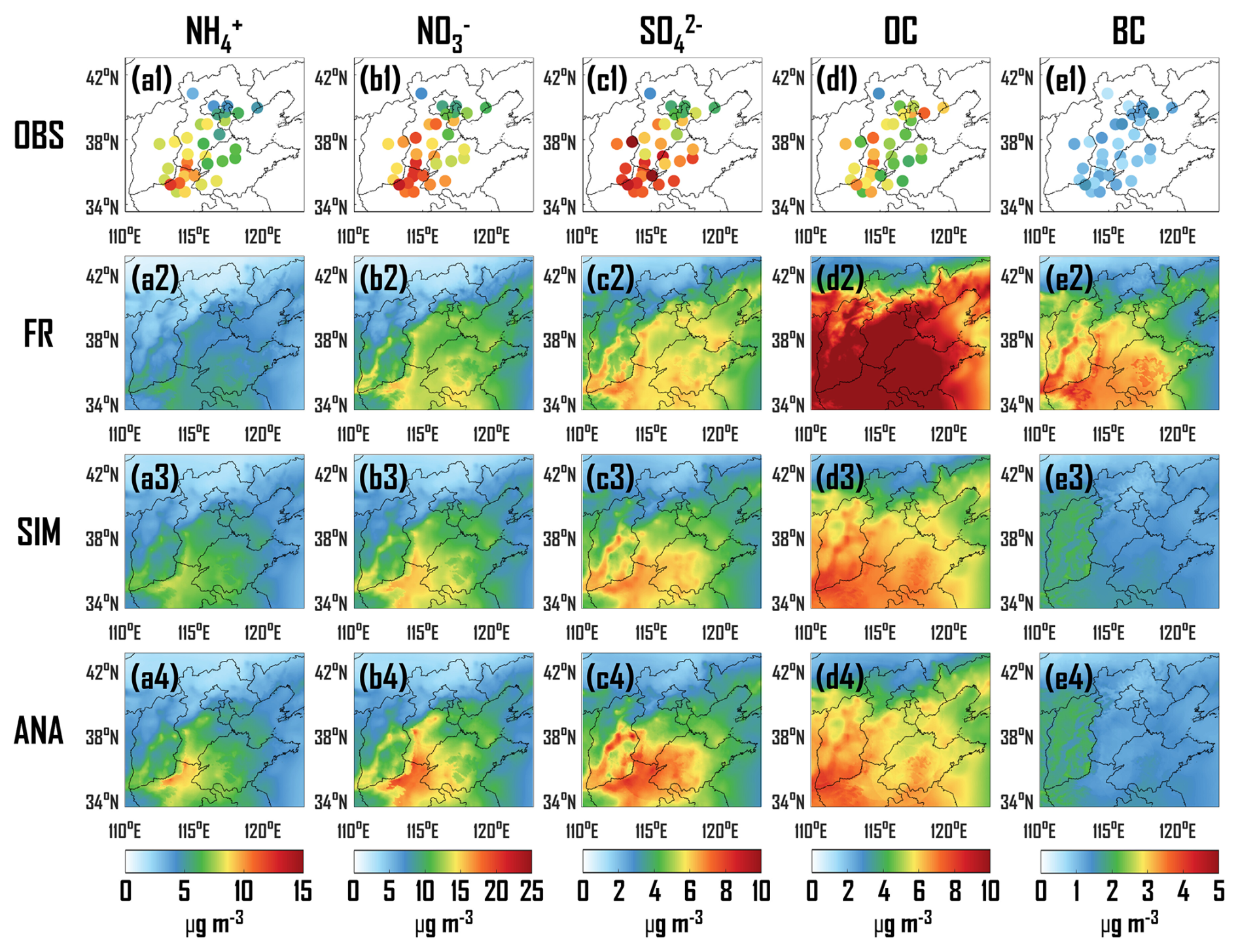
Figure 6 Spatial distribution of observation (OBS), free-run field (FRFR), ML-simulated background field (SIM) and analysis field (ANA) for NH${}_{\mathrm{4}}^{+}$ (a1–a4), NO${}_{\mathrm{3}}^{-}$ (b1–b4), SO${}_{\mathrm{4}}^{\mathrm{2}-}$ (c1–c4), OC (d1–d4) and BC (e1–e4).

3.3.2 Assessment of spatial distribution in chemical components

Figure 6 presents the spatial distributions of observations from sparse sites (OBS), FR, SIM and ANA for the average concentrations of NH${}_{\mathrm{4}}^{+}$, NO${}_{\mathrm{3}}^{-}$, SO${}_{\mathrm{4}}^{\mathrm{2}-}$, OC, and BC over a two-month period from February to March 2022. The OBS of NH${}_{\mathrm{4}}^{+}$ reveals that the concentrations at southern sites in North China are significantly higher than those at northern sites, particularly in northern Henan Province, with a maximum concentration of 12.20 µg m⁻³ (Fig. 6a1). However, FR fails to accurately capture the spatial patterns of NH${}_{\mathrm{4}}^{+}$ concentration (Fig. 6a2), exhibiting underestimations at 100 % of DA sites and 89 % of VE sites, with average underestimations of 2.71 and 3.07 µg m⁻³, respectively (Fig. 7a1). This finding is attributed to the underestimation of the original training samples (Kong et al., 2025). Compared to FR, the SIM mitigates the underestimation (Fig. 6a3), with 96 % of DA sites underestimating by 1.56 µg m⁻³ and 78 % of VE sites underestimating by 1.88 µg m⁻³ (Fig. 7a2). After DA, ANA accurately depicts the spatial distribution of NH${}_{\mathrm{4}}^{+}$ concentrations (Fig. 6a4), with 92 % of DA sites underestimating by 0.74 µg m⁻³ and 44 % of VE sites underestimating by 2.34 µg m⁻³, respectively (Fig. 7a3). The increment field (INC) between ANA and SIM exhibits substantial positive increments in southern North China (Fig. 7a4), indicating that the observations from 24 DA sites were effectively propagated within the model state space, thereby addressing the underestimation of NH${}_{\mathrm{4}}^{+}$ concentrations in the whole domain.

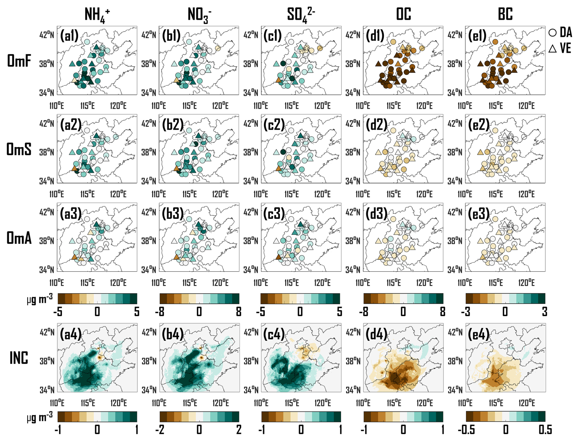
Figure 7 Spatial distribution of observation minus free-run field (OmF), observation minus ML-simulated background field (OmS), observation minus analysis field (OmA) and analysis field minus background field (INC) for NH${}_{\mathrm{4}}^{+}$ (a1–a4), NO${}_{\mathrm{3}}^{-}$ (b1–b4), SO${}_{\mathrm{4}}^{\mathrm{2}-}$ (c1–c4), OC (d1–d4) and BC (e1–e4). The circle indicates the DA sites with data assimilation, and the upward-pointing triangle indicates the VE sites without data assimilation.

The observed spatial distributions of NO${}_{\mathrm{3}}^{-}$ and SO${}_{\mathrm{4}}^{\mathrm{2}-}$ are consistent with those of NH${}_{\mathrm{4}}^{+}$, revealing significantly higher concentrations at southern sites in the North China region than at northern sites, particularly in the Hebei-Henan-Shandong junction areas (Fig. 6b1 and c1). Although FR can capture the spatial patterns of NO${}_{\mathrm{3}}^{-}$ and SO${}_{\mathrm{4}}^{\mathrm{2}-}$, it significantly underestimates their concentrations (Fig. 6b2 and c2). Specifically, 63 %–79 % of DA sites and 89 % of VE sites underestimate by 1.87–3.76 and 1.57–3.44 µg m⁻³, respectively (Fig. 7b1 and c1). Compared to FR, SIM mitigates the underestimations in the Hebei-Henan-Shandong junction areas and overestimations in the Beijing-Tianjin-Hebei eastern areas (Fig. 6b3 and c3), with improvements at most DA and VE sites (Fig. 7b2 and c2). After DA, ANA accurately characterizes the spatial distribution of NO${}_{\mathrm{3}}^{-}$ and SO${}_{\mathrm{4}}^{\mathrm{2}-}$ concentrations (Fig. 6b4 and c4), with 88 %–100 % of DA sites and 56 %–67 % of VE sites merely underestimating by 0.77–1.31 and 1.85–2.73 µg m⁻³, respectively (Fig. 7b3 and c3). Furthermore, similar to the INC of NH${}_{\mathrm{4}}^{+}$, INCs of NO${}_{\mathrm{3}}^{-}$ and SO${}_{\mathrm{4}}^{\mathrm{2}-}$ exhibit widespread positive increments across the North China region (Fig. 7b4 and c4).

In contrast to the spatial distributions of NH${}_{\mathrm{4}}^{+}$, NO${}_{\mathrm{3}}^{-}$ and SO${}_{\mathrm{4}}^{\mathrm{2}-}$, the observed spatial distributions of OC and BC reveal that concentrations in the North China region demonstrate spatial homogeneity (Fig. 6d1 and e1). However, FR significantly overestimated the concentrations of OC and BC in the North China region (Figs. 6d2, e2, and 7d1, e1), with an average overestimation of 6.12 µg m⁻³ for OC and 1.99 µg m⁻³ for BC at all DA sites, and 6.88 µg m⁻³ for OC and 2.29 µg m⁻³ for BC at all VE sites. Following incremental learning, SIM significantly reduced the overestimations (Figs. 6d3, e3, and 7d2, e2), resulting in an average overestimation of 1.46 µg m⁻³ for OC and 0.53 µg m⁻³ for BC at 71 %–79 % of DA sites, and 1.56 µg m⁻³ for OC and 0.65 µg m⁻³ for BC at 89 % of VE sites. The number of sites exhibiting overestimation and the degree of overestimation are markedly lower than those of FR. After DA, ANA further mitigates the overestimation in SIM, accurately interpreting the spatial distributions of OC and BC concentrations (Fig. 6d4 and e4), with the gaps between the observations and analysis fields for both DA and VE sites approaching 0 (Fig. 7d3 and e3). Assimilating the observations from 24 DA sites effectively mitigates the overestimation in the southern North China region (Fig. 7d4 and e4).

3.3.3 Comparison with multiple reanalysis datasets

In this section, we utilized OIRF-LEnKF v1.0 to generate an hourly reanalysis dataset of PM_2.5 key chemical components (SO${}_{\mathrm{4}}^{\mathrm{2}-}$, NO${}_{\mathrm{3}}^{-}$, NH${}_{\mathrm{4}}^{+}$, OC and BC) for the North China region in February 2022. We compared it with multiple related reanalysis datasets, including CAQRA-aerosol, TAP, Global-RA (CAMS and MERRA-2), and the dataset generated by NP2. The temporal and spatial resolutions of CAQRA-aerosol, TAP, and Global-RA on both global and national scales are lower than those of OIRF-LEnKF v1.0 and NP2 on the regional scale (Table 2). It is important to note that the spatial range and resolution of OIRF-LEnKF v1.0 are contingent upon those of the available training data. Consequently, OIRF-LEnKF v1.0 has significant potential for elucidating the spatiotemporal distribution of PM_2.5 chemical components on a global and national scale.

Figure 8 illustrates the average values of observation minus analysis (OmA) over 1 month. For NH${}_{\mathrm{4}}^{+}$ (Fig. 8a1–a5), the mean absolute OmA of OIRF-LEnKF v1.0 at a total of 33 sites (0.25 µg m⁻³) is significantly lower than that of NP2 (0.81 µg m⁻³), CAQRA (1.18 µg m⁻³), TAP (0.92 µg m⁻³), and Global-RA (2.92 µg m⁻³). Furthermore, the OmA of OIRF-LEnKF v1.0 is within ±1 µg m⁻³ at 97 % of the sites, whereas NP2, CAQRA, TAP, and Global-RA had only 9 %–70 % of the sites within this range. Most of the sites exhibit slight underestimations in NP2 and TAP, overestimations in CAQRA, and significant underestimations in Global-RA, while the disparity between OIRF-LEnKF v1.0 and the observations is minimal. The findings for NO${}_{\mathrm{3}}^{-}$ are comparable to those for NH${}_{\mathrm{4}}^{+}$ (Fig. 8b1–b5), the mean absolute OmA of OIRF-LEnKF v1.0 at a total of 33 sites (0.19 µg m⁻³) is significantly lower than that of NP2 (0.93 µg m⁻³), CAQRA (8.42 µg m⁻³), TAP (2.24 µg m⁻³), and Global-RA (2.27 µg m⁻³). Furthermore, the OmA of OIRF-LEnKF v1.0 is within ±2 µg m⁻³ at all sites, whereas NP2, CAQRA, TAP, and Global-RA had only 3 %–94 % of the sites within this range. The similar spatial patterns of OmA for NH${}_{\mathrm{4}}^{+}$ and NO${}_{\mathrm{3}}^{-}$ are related to thermodynamic equilibrium (Nenes et al., 1998) and consistency between NH${}_{\mathrm{4}}^{+}$ and NO${}_{\mathrm{3}}^{-}$ has also been observed in previous works (Sun, 2018; Shi et al., 2021; Wu et al., 2022).

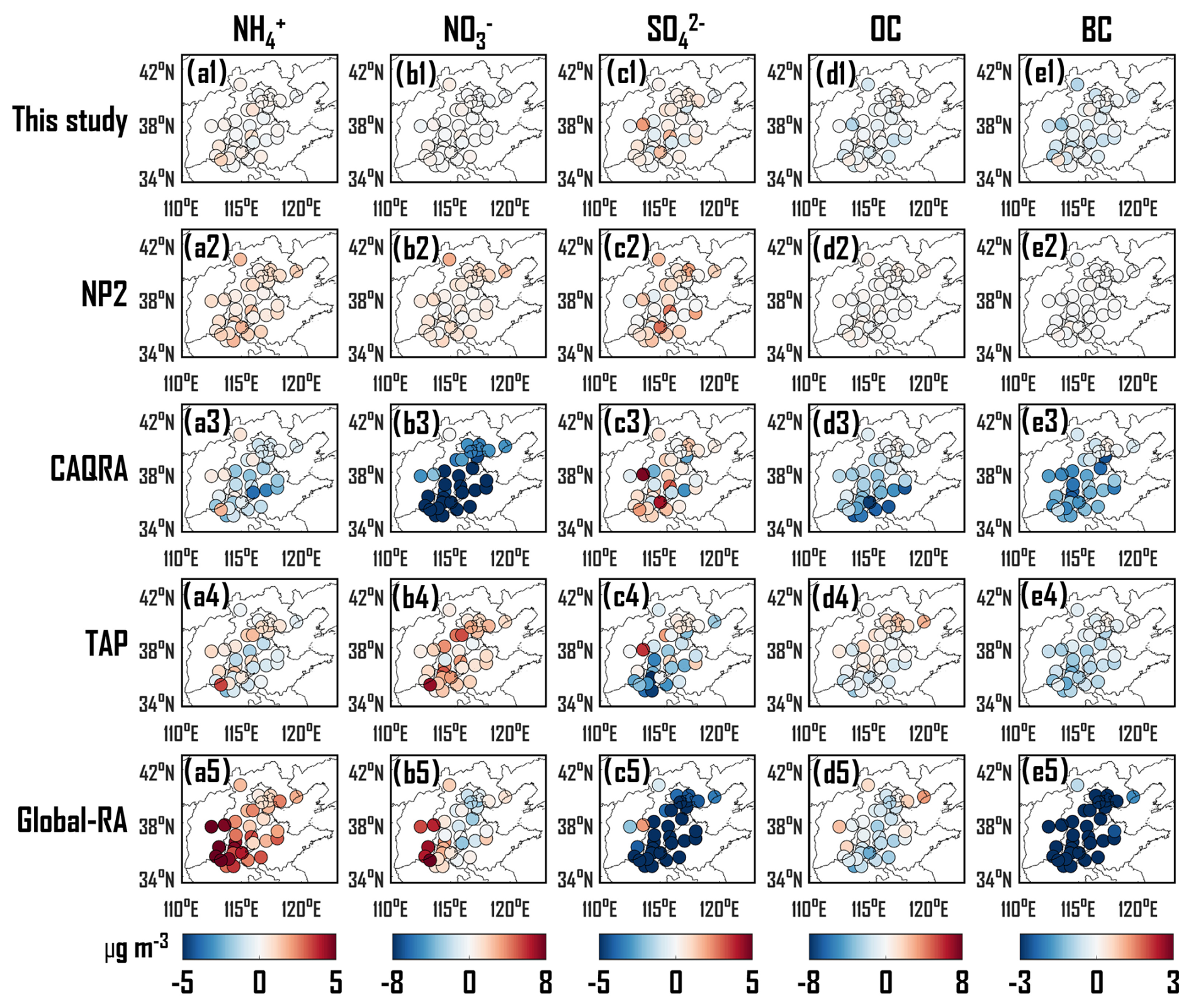
Figure 8 Difference between observations at a total of 33 sites and five reanalysis datasets for NH${}_{\mathrm{4}}^{+}$ (a1–a5), NO${}_{\mathrm{3}}^{-}$ (b1–b5), SO${}_{\mathrm{4}}^{\mathrm{2}-}$ (c1–c5), OC (d1–d5) and BC (e1–e5). Global-RA is the combination of CAMSRA and MERRA-2.

For SO${}_{\mathrm{4}}^{\mathrm{2}-}$ (Fig. 8c1–c5), the average absolute OmA of OIRF-LEnKF v1.0 (0.54 µg m⁻³) is slightly lower than that of NP2 (0.86 µg m⁻³) but significantly lower than that of CAQRA (1.26 µg m⁻³), TAP (1.72 µg m⁻³), and Global-RA (7.19 µg m⁻³). In contrast to NO${}_{\mathrm{3}}^{-}$, most of the sites exhibit underestimation in CAQRA, overestimation in TAP, and significant overestimation in Global-RA for SO${}_{\mathrm{4}}^{\mathrm{2}-}$. This discrepancy between NO${}_{\mathrm{3}}^{-}$ and SO${}_{\mathrm{4}}^{\mathrm{2}-}$ arises from the competition for the capture of NH₃. Thus, the underestimation of SO${}_{\mathrm{4}}^{\mathrm{2}-}$ is considered a factor in the overestimation of NO${}_{\mathrm{3}}^{-}$ (Xie et al., 2022). Unlike the four CTM-based reanalysis datasets, OIRF-LEnKF v1.0 implements independent simulation and DA processes for various chemical components, thereby reducing the constraints imposed by correlations among variables.

The OmA of OC (Fig. 8d1–d5) and BC (Fig. 8e1–e5) exhibit similar spatial patterns. Specifically, the average absolute OmA of OIRF-LEnKF v1.0 (0.66 µg m⁻³ for OC and 0.40 µg m⁻³ for BC) is slightly higher than that of NP2 (0.23 µg m⁻³ for OC and 0.03 µg m⁻³ for BC) but significantly lower than those of CAQRA (2.90 µg m⁻³ for OC and 1.32 µg m⁻³ for BC), TAP (1.04 µg m⁻³ for OC and 0.65 µg m⁻³ for BC), and Global-RA (1.62 µg m⁻³ for OC and 5.85 µg m⁻³ for BC). The significant overestimation of carbonaceous aerosols observed in CTM-based CAQRA and Global-RA is likely attributed to the hygroscopic growth schemes of carbonaceous aerosols, the poorly constrained semi-volatile species that escape from primary organic aerosols, and aging mechanisms (Soni et al., 2021; Huang et al., 2013). Overall, the reanalysis dataset generated by OIRF-LEnKF v1.0 demonstrates lower errors in the concentrations of the five PM_2.5 chemical components in the North China region compared to four CTM-based datasets.

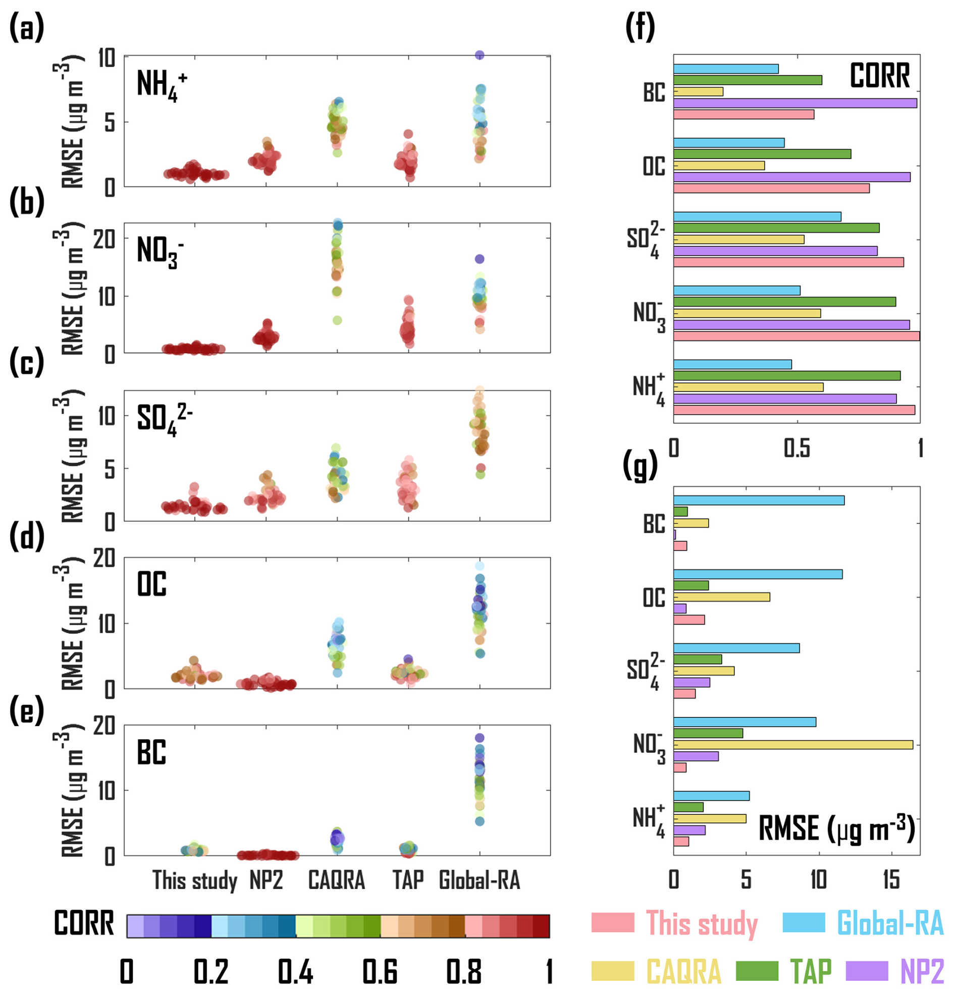
Figure 9 Pearson correlation coefficient (CORR) and root mean square error (RMSE, µg m⁻³) quantified by the five reanalysis datasets and observations at a total of 33 sites for NH${}_{\mathrm{4}}^{+}$ (a), NO${}_{\mathrm{3}}^{-}$ (b), SO${}_{\mathrm{4}}^{\mathrm{2}-}$ (c), OC (d) and BC (e). The averages of CORR (f) and RMSE (g) across all observational sites for the five reanalysis datasets for the five PM_2.5 chemical components. Global-RA is the combination of CAMSRA and MERRA-2.

We further compared the differences in RMSE and CORR among five reanalysis datasets. As illustrated in Fig. 9a–c, the CORR values of OIRF-LEnKF v1.0 for NH${}_{\mathrm{4}}^{+}$, NO${}_{\mathrm{3}}^{-}$, and SO${}_{\mathrm{4}}^{\mathrm{2}-}$ (mean CORR: 0.97, Fig. 9f) are significantly higher than those of other datasets (mean CORR: 0.56 to 0.89, Fig. 9f), while the RMSE values (mean RMSE: 1.12 µg m⁻³, Fig. 9g) are significantly lower than those of other datasets (mean RMSE: 2.55–8.52 µg m⁻³, Fig. 9g). Furthermore, the RMSE values of OIRF-LEnKF v1.0 are relatively concentrated across all sites, indicating a marked improvement in simulation of NH${}_{\mathrm{4}}^{+}$, NO${}_{\mathrm{3}}^{-}$, and SO${}_{\mathrm{4}}^{\mathrm{2}-}$ across a broad spatial range. From Fig. 9d and e, the CORR and RMSE values of OIRF-LEnKF v1.0 for carbonaceous aerosols (OC and BC) (mean CORR: 0.68, Fig. 9f; mean RMSE: 1.49 µg m⁻³, Fig. 9g) are slightly worse than those of NP2 (mean CORR: 0.97, Fig. 9f; mean RMSE: 1.66 µg m⁻³, Fig. 9g) and are comparable to those of TAP (mean CORR: 0.66, Fig. 9f; mean RMSE: 1.49 µg m⁻³, Fig. 9g), while demonstrating superiority over the other datasets (mean CORR: 0.28–0.44, Fig. 9f; mean RMSE: 4.49–11.70 µg m⁻³, Fig. 9g). Overall, OIRF-LEnKF v1.0 exhibits a notable advantage in accurately interpreting the concentrations of PM_2.5 chemical components on a regional scale. Further improvements in the performance of OIRF-LEnKF v1.0 in interpreting carbonaceous aerosols are expected by modifying the structure of the OIRF model and the frequency of incremental learning, as well as by adopting hybrid nonlinear DA algorithms.

3.4 Limitations

Although the OIRF model serves as an efficient surrogate for the CTM in generating simulation or forecast ensembles for data assimilation, it inherits a constrained extrapolation capability of tree-based models. Specifically, the OIRF model may exhibit a tendency to saturate at learned extremes when extrapolating beyond its training data distribution, which directly limits its generalizability in diverse and complex atmospheric scenarios, such as the pollution extremes in seasons outside the training period. The poor performance of tree-based models on testing sets has been reported in our previous study (Li et al., 2025). Our incremental learning mechanism is designed to mitigate the extrapolation limitation by dynamically updating the RF model with new knowledge. However, the effectiveness of incremental learning is contingent upon the availability of high-quality analysis fields. A lack of observations, which prevents the generation of analysis fields, exposes the OIRF model to its inherent extrapolation limitations, leading to compromised simulation accuracy.

Replacing the RF model with an ensemble of deep neural networks (DNNs) holds promise for superior nonlinear mapping and extrapolation. However, the considerably higher computational cost required for both training and inference of DNNs (Debjyoti and Utpal, 2025; Xi, 2022) results in an operational bottleneck that the process of updating and running an ensemble of DNNs can be slower than traditional CTM-based ensemble simulations, which could offset its accuracy advantages. Therefore, balancing the inherent predictive performance of a machine learning model against its computational cost remains a central challenge for the practical online coupling of machine learning with data assimilation.

4 Conclusions

In this paper, we online coupled the OIRF model with the LEnKF algorithm to develop a novel DA system (OIRF-LEnKF v1.0) that mitigates the limitations of high computational costs and inadequate advancements in generating background and analysis fields of PM_2.5 chemical components (NH${}_{\mathrm{4}}^{+}$, SO${}_{\mathrm{4}}^{\mathrm{2}-}$, NO${}_{\mathrm{3}}^{-}$, OC and BC) in conventional CTM-based DA. The OIRF model introduces an incremental learning mechanism that enhances the generalization ability of ML by iteratively absorbing newly available training data to dynamically update the model structure. The domain localization and observation localization schemes are incorporated into the EnKF algorithm within a second-level parallel computation framework, which effectively reduces the interference of spatial and variable spurious correlations and improves computational efficiency. The findings are outlined as follows.

OIRF-LEnKF v1.0 exhibits stable convergence capability and high convergence efficiency, achieving convergence within 10 iterations across ensemble sizes ranging from 2 to 200. Computational tests reveal that the total time consumed by OIRF-LEnKF v1.0 constitutes only 11.41 %–16.60 % of that of CTM-based DA, primarily because the simulation process requires only 0.13 % to 0.20 % of the CTM computation time, demonstrating its superior computational efficiency.

Sensitivity tests reveal that the background fields in OIRF-LEnKF v1.0 are more sensitive to updating frequency within the incremental learning mechanism. In contrast, the analysis fields exhibit a marked sensitivity to ensemble size. Specifically, the ΔCORR rises by 2.43 %–11.75 %, and the ΔRMSE decreases by 32.55 %–40.36 % when comparing a 1 h update frequency to the scenario without incremental learning during the simulation phase. Additionally, the ΔCORR increases by 9.75 %–19.04 %, and the ΔRMSE decreases by 16.70 %–30.48 % when comparing an ensemble size of 200 to that of 20 during the DA analysis phase. However, the 1 h update frequency diminishes the dependence of the analysis fields on ensemble size. Thus, an ensemble size of 50 with a 6 h update frequency is configured to balance computational efficiency, ML simulation accuracy, and DA analysis performance.

A 2-month DA experiment demonstrates that the RMSE values for PM_2.5 chemical components at DA sites range from 0.99 to 7.80 µg m⁻³ after incremental learning and 0.80 to 2.36 µg m⁻³ after DA analysis, exhibiting reductions of 26.38 %–61.75 % and 68.99 %–91.31 %, respectively, compared to values obtained without incremental learning and DA analysis. For VE sites, the RMSE values range from 0.93 to 7.76 µg m⁻³ after incremental learning and 0.90 to 7.76 µg m⁻³ after DA analysis, exhibiting reductions of 28.37 %–68.00 % and 23.46 %–68.75 %, respectively, relative to values obtained without incremental learning and DA analysis. Notably, the RMSE values of our system during the simulation process show a significant reduction of 33.16 %–90.10 % at DA sites and 37.10 %–91.55 % at VE sites compared to those of CTM-based DA, highlighting the superior simulation capability of ML-based DA. Additionally, the spatial patterns of the background and analysis fields for chemical components more accurately reflect those of the observations when employing incremental learning and DA.

In comparison to the datasets provided by NP2, CAQRA, TAP, CAMSRA, and MERRA-2, the dataset generated by OIRF-LEnKF v1.0 exhibits superior data quality. Notably, for NH${}_{\mathrm{4}}^{+}$, NO${}_{\mathrm{3}}^{-}$ and SO${}_{\mathrm{4}}^{\mathrm{2}-}$, the CORR values of OIRF-LEnKF v1.0 (0.97) are significantly higher than those of the aforementioned datasets (0.56–0.89). Additionally, the RMSE values of OIRF-LEnKF v1.0 (1.12 µg m⁻³) are markedly lower than those of the four reanalysis datasets (2.55–8.52 µg m⁻³). Future work should focus on generating reanalysis datasets that utilize configurations with larger domains and higher spatial resolutions, as well as improving data quality through the application of deep learning techniques and hybrid nonlinear DA algorithms.