Applying corrective machine learning in the E3SM atmosphere model in C+ +  (EAMxx)

The Simple Cloud-Resolving E3SM Atmosphere Model (SCREAM) is the newest addition to the family of earth system models capable of explicitly resolving convective systems. SCREAM is a kilometer-scale configuration of the advanced E3SM Atmosphere Model (EAMxx), designed for heterogeneous computing architectures. While the enhanced accuracy of kilometer-scale modeling offers significant benefits, it comes with a substantial computational cost, limiting feasible simulation durations to only a few years to a few decades, even on the fastest supercomputers. Machine learning presents an opportunity for scientists to achieve the high accuracy of storm-resolving models at a significantly reduced cost. Building on the previous success of applying corrective machine learning (ML) to the FV3GFS earth system model, this study explores the effects of implementing corrective-ML in EAMxx-SCREAM. We also address the computational challenges of integrating our implementation of corrective-ML, which is written in Python, with the C$++$/Kokkos EAMxx driver, as well as potential reasons why this approach has not proved as effective for EAMxx-SCREAM as for FV3GFS.

1 Introduction

Accurate future climate projections are crucial to a variety of sectors, including agricultural, energy, and public health. For instance, they can help predict shifts in growing seasons, optimize renewable energy deployment, and improve understanding of climate-sensitive diseases. Currently, physics-based earth system models, also referred to as general circulation models (GCMs), are responsible for generating these projections and require a massive amount of computing resources in order to produce one climate realization (Hohenegger et al., 2023). These models need to balance accuracy with feasibility, and most opt to use coarse spatial resolution, typically around 100 km, allowing them to produce ensembles of climate simulations for decades or centuries. However, the downside of using coarse-resolution GCMs is their inability to resolve storms, clouds, and complex topography (Satoh et al., 2019). The Simple Cloud-Resolving E3SM Atmosphere Model (SCREAM) addresses the resolution problem by using kilometer-scale resolution, but it is too computationally expensive to run more than a few years at a time (Caldwell et al., 2021). This project aims to apply a computationally efficient machine learning (ML) based emulator of high-resolution SCREAM nudging tendencies, thus replicating the high accuracy of the cloud-resolving GCM at the reduced computational cost of the coarse-resolution GCM.

ML has the potential of revolutionizing how weather forecasts and climate predictions are generated (Eyring et al., 2024). Within this active area of research, there are two primary approaches. The first approach relies solely on ML models trained on historical observations, reanalysis datasets, or outputs from existing GCMs (Keisler, 2022; Chen et al., 2023; Lam et al., 2023; Price et al., 2023). The second approach involves a hybrid framework that combines machine learning with traditional GCMs. In this method, machine learning methods are often used to replace a specific physical process of GCMs (Kochkov et al., 2023; Henn et al., 2024; Hu et al., 2025) or to apply column-wise correction to the coarse-grid GCM (Bretherton et al., 2022). This study builds on the success of a study using the second approach by the Allen Institute for Artificial Intelligence (Ai2) working with the Finite-Volume Cubed-Sphere Global Forecast System (FV3GFS) GCM (https://github.com/ai2cm/fv3gfs-fortran, last access: 9 July 2024) (Zhou et al., 2019). Ai2 was able to improve the predictive accuracy of relatively coarse-resolution global simulations using a machine-learning based correction to the atmosphere state (Bretherton et al., 2022; Kwa et al., 2023; Sanford et al., 2023).

This study applies their corrective-ML approach to SCREAM. In addition, it developed software infrastructure that will be helpful for subsequent studies coupling ML to SCREAM. Section 2 provides the recipe for the development of the ML training data. Section 3 covers how the corrective-ML model was embedded into the SCREAM code base. Section 4 examines how well the ML-corrected coarse GCM performs with respect to the fine-resolution target, followed by discussion of the results and conclusions of the study in Sects. 5 and 6.

2 Methods

SCREAM is a configuration of the atmosphere component of the Energy Exascale Earth System Model (E3SM) targeting kilometer-scale global resolutions. In order to accomplish performant simulations at this scale, the E3SM Atmosphere Model (EAMxx) was rewritten from the original Fortran code to C$++$/Kokkos (Donahue et al., 2024). The adoption of Kokkos (Carter-Edwards et al., 2014) in EAMxx unlocks the computational power of mixed CPU/GPU machines and ensures that EAMxx maintains good performance across a number of high performance computing systems (Donahue et al., 2024). EAMxx employs a spectral-element, nonhydrostatic dynamical core for resolved-scale processes (Taylor et al., 2020). Major subgrid physics parameterizations include P3 microphysics (Morrison and Milbrandt, 2015), SHOC turbulence and boundary layer physics (Bogenschutz and Krueger, 2013), and RRTMG++ radiation (Pincus et al., 2019). Notably, the SCREAM configuration omits a deep convection parameterization, regardless of grid resolution (Caldwell et al., 2021). For all simulations in this work, the model configuration and initial start date are identical. Initial conditions for all simulations are generated from ERA5 (Hersbach et al., 2020).

While EAMxx achieves computational performance of more than one simulated year per wallclock day for a km-scale GCM (Taylor et al., 2023), its computational cost is still prohibitive for global km-scale simulations of a decade or more in length. This limitation makes it attractive to apply corrective-ML to EAMxx in order to represent effects of fine scale features at coarse resolution. We follow Ai2's approach with FV3GFS (Bretherton et al., 2022), using a km-scale EAMxx simulation to produce fine-scale training data for a corrective-ML model embedded in coarse-resolution EAMxx simulations. The approach is modified to handle technical and architectural differences between FV3GFS and EAMxx, see Sects. 2.1 and 2.2 for more details.

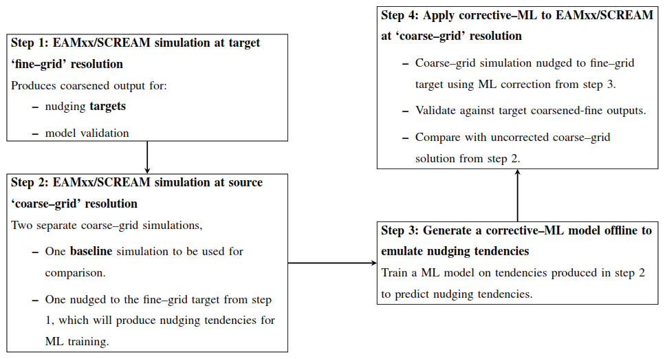
Figure 1 Flow diagram for training and applying the corrective machine learning (ML) model, which uses ML predicted nudging tendencies (step 3) to correct coarse-scale E3SM simulations (step 4). For this study “coarse-grid” resolution refers to 100 km global resolution and “fine-grid” resolution refers to 3 km global resolution. All simulations are conducted using the Simple Cloud-Resolving E3SM Atmosphere Model (SCREAM) configuration of the E3SM Atmosphere Model in C$++$/Kokkos (EAMxx).

The corrective-ML approach described in this study can be represented by four steps (Fig. 1). The first step involves the generation of a fine-grid reference simulation. This simulation serves two purposes: to provide the nudging targets for the training data set and to provide a validation data set for the ML-corrected solution. The second step involves nudging an EAMxx simulation at coarse resolution to the reference state. “Nudging tendencies” derived from this step are used for the third step, training of the corrective-ML models. Finally, a coarse-grid EAMxx simulation is run with inline corrections from these ML models; ideally the resulting ML-corrected coarse GCM will more closely approximate the time evolution and solution of the target fine-grid GCM. Each of these steps is described in more detail in the following subsections.

All tunable model parameters are held fixed between the coarse- and fine-resolution simulations, so in every case the parameter space is consistent with that of the target fine-resolution simulation. As a result, the climate states of the untuned coarse simulations would likely diverge from the fine resolution over long timescales. However, this study focuses on the shorter timescale of one year. We therefore expect the coarse simulations, when nudged toward the fine-resolution state, to agree more closely with the fine-resolution simulation.

2.1 A km-scale reference solution

For the training and validation discussed in this paper, we used one year of customized outputs from a reference fine-grid simulation using the default SCREAM configuration of EAMxx (Donahue et al., 2024). This used a cubed-sphere spectral-element grid for the dynamics calculation which had a number of elements per cube face of 1024 × 1024. Each element contains a physics grid with a 2 × 2 arrangement of columns. Referred to in shorthand as the “ne1024pg2” horizontal grid, this grid has approximately 3.25 km horizontal resolution, 128 vertical levels, and a physics timestep of 100 s.

The 1-year simulations in this study follow the “standard climate” configuration of a Cess-style SCREAM simulation pair further discussed by Terai et al. (2025). It started on 1 August 2019 and used a climatological seasonal cycle of sea-surface temperature (SST) and sea ice. The Terai et al. (2025) study provided the fine-resolution data for training and validation.

Table 1 List of variables used for the 100 km to 3 km nudged simulations.Column 1 is the typical variable description, column 2 is the variable name as provided in EAMxx output files, column 3 is the units of the variable, column 4 describes the dimensionality of the variable. 2D has no vertical extent, 3D has vertical layers. Column 5 states if the variable was nudged or prescribed in the nudged simulation. Surface variables were prescribed.

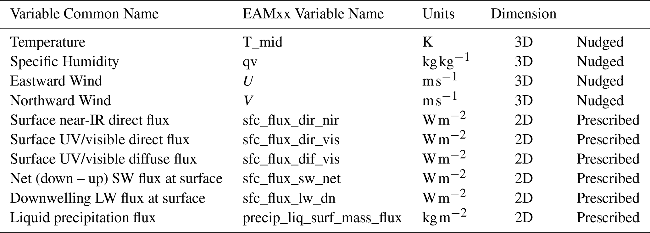
Table 2 List of variables from the nudged simulation used for validation of the corrective-ML model. Column 1 is the typical variable description, column 2 is the variable name as provided in EAMxx output files, column 3 is the units of the variable and column 4 describes the dimensionality of the variable. 2D has no vertical extent, 3D has vertical layers.

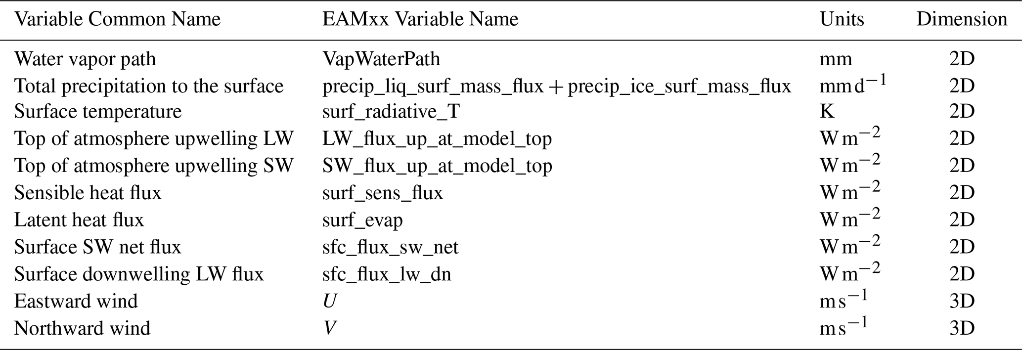
Temporally averaged SCREAM output was produced every 3 h. Three-dimensional fields required for our ML study were vertically interpolated natively in SCREAM onto a set of fixed pressure levels (specified below), then horizontally averaged (area-weighted) along pressure surfaces to a target “ne30pg2” (≈ 100 km) coarse grid, masking fine-grid points below the surface. Two dimensional ML-relevant fields such as surface precipitation were also horizontally averaged inline to the “ne30pg2” grid. Only these horizontally coarsened 3D and 2D outputs were stored. Training data was produced from a 100 km simulation that was nudged to the 3 km state, see Sect. 2.2 for details. Table 1 lists the variables used for nudging. Table 2 list all variables output for validation of the ML model.

The vertical grid used for pressure interpolation has 221 vertical levels. Starting with a lowest level of 1075 hPa, each subsequent level decreases by 5 hPa until 540 hPa. From 540 to 270 hPa the spacing is 10 hPa, and from 270 to 145 hPa the spacing is again 5 hPa. For the remainder of the upper atmosphere, the vertical grid uses the upper 60 typical isobaric vertical layers in an EAMxx grid, for a total of 221 layers. The interpolated data is masked for below-surface pressure levels, which is particularly important in mountainous terrain. The horizontal area-weighted averaging from the fine to the coarse grid is performed using the Tempest remap algorithm (Ullrich and Taylor, 2015; Ullrich et al., 2016), which efficiently redistributes data across different grid resolutions.

The approach to vertical remapping in this study differs from that used in the FV3GFS study. There, fine-grid data were vertically interpolated to the local pressure levels of the coarse-resolution data, masking out fine-grid data at any resulting grid points below the surface (since the FV3GFS model levels are terrain-following, these pressure levels differ between coarse grid cells). They then used the same method for horizontal coarsening as we do (Bretherton et al., 2022). Our coarse-grid ne30pg2 EAMxx configuration has only 72 terrain-following vertical levels, rather than the 128 levels of the fine-grid configuration. In the FV3GFS application, the coarse- and fine-grid model versions had the same set of vertical levels.

To maintain hydrostatic balance and conserve atmospheric mass during the vertical interpolation and horizontal coarsening process, the FV3GFS study also applied a small correction to the area-weighted surface elevation, which we neglect. See Sect. 2.4 in Bretherton et al. (2022) for more details.

For the FV3GFS study, instantaneous 3-hourly snapshots of the prognostic fields were stored, rather than the 3-hourly average fields used here. Our approach produces smoother nudging tendencies, whereas the FV3GFS approach has the interpretational advantage that 3-hourly average tendencies are simply differences between successive 3-hourly snapshots.

2.2 Machine learning training data – nudged simulation

Similar to the work with FV3GFS (Bretherton et al., 2022), our training dataset for corrective-ML was constructed from a “low-resolution” 100 km global simulation that was nudged to track the vertically interpolated and horizontally coarsened reference solution evolution described in Sect. 2.1. At the end of each atmospheric timestep, the atmosphere state was adjusted to match the fine-resolution solution state using data from the reference simulations, with a nudging timescale of 3 h. At each timestep, the reference data was interpolated to the current time before nudging.

EAMxx employs a hybrid pressure coordinate system vertically (Dennis et al., 2005), thus the reference data also required vertical interpolation from its fixed vertical pressure grid onto the EAMxx pressure coordinates at each timestep. For the training dataset simulation, only the three-dimensional variables – temperature, specific humidity, and horizontal velocities – were nudged. The other surface variables, as detailed in Table 1, were directly prescribed at the end of the atmospheric timestep. The nudging tendencies from this simulation were averaged every 3 h and written to output. In addition, the training data requires a record of the atmosphere state that led to each nudging tendency, recorded at the same 3-hourly times as the tendencies.

2.3 Training the model

Following Ai2's prior work with FV3GFS, the nudging tendencies recorded during the nudged simulation discussed in Sect. 2.2 are used to train three separate corrective-ML models for different state variables in EAMxx. All models utilize the Ai2 Climate Modeling Group's open-source fv3net GitHub repository (Donahue and Wu, 2025a). The training process is column-independent, meaning that each training data point does not consider neighboring spatial columns in the grid. However, the training dataset does include some grid location information through the latitude and cosine zenith angle associated with each point. Below, we outline the parameters for each model.

1. Thermodynamic Model: This model focuses on the thermodynamic state of the atmosphere. The input variables for training include temperature, specific humidity, latitude, surface geopotential, and cosine zenith angle. The training outputs are the prescribed nudging tendencies for temperature and specific humidity. We follow Kwa et al. (2023) where a fully-connected dense network with 3 hidden layers with 419 neurons per layer is used.

2. Momentum Model: This model targets the atmospheric momentum state. The outputs are the eastward and northward velocity nudging tendencies. The input variables are the same as those used in the thermodynamic model, with the addition of eastward and northward velocity. This model uses the same dense network as the thermodynamic model.

3. Surface Forcing Model: This model addresses the surface forcing passed to other components of the earth system. Unlike the other models, it does not use nudging tendencies as input. Instead, it relies on the prescribed surface fluxes calculated in the reference solution. The inputs for this model match those of the thermodynamic model, while the outputs are the surface downwelling longwave flux and surface net shortwave flux broken down into near-infrared and visible direct and diffuse flux fraction. Like the thermodynamic model, this model also uses the same dense network. We apply output limiters to ensure physical consistency (e.g., downward near-infrared diffuse fraction is between 0–1).

All models are trained for 300 epochs, with an early stopping condition if convergence is detected. Random subsets of dates from the EAMxx dataset are selected for training and validation.

2.4 Coarse-grid GCM

The three machine learning models developed in Sect. 2.3 are integrated into EAMxx to create a coarse-grid GCM that aspirationally produces solutions closer to fine-grid accuracy. For more details on how the ML models were embedded in the EAMxx code base please refer to the section on Python/C$++$ coupling, Sect. 3. The corrective-ML is applied at the end of each atmospheric timestep, with the thermodynamic and momentum models operating independently but using the same model input state. The surface forcing model updates the surface fluxes based on the ML-corrected state. The set of variables saved for validation of the ML-corrected solution is given in Table 2.

Special care is needed when applying corrections from the thermodynamic model. Nudging specific humidity effectively adds or removes water vapor mass from the system, which typically reflects precipitation differences in the fine-resolution solution compared with the coarse-resolution solution. To account for this, the total change to the column water mass is calculated after adjusting specific humidity, and this result is then added to or subtracted from the total liquid precipitation. A mass clipper, in which negative values are set to zero, is employed to ensure that precipitation values remain non-negative. This correction method does not account for ice precipitation. Future studies could explore separate ice and liquid precipitation adjustments, depending e.g. on near-surface air temperature. For the short simulations considered in this study, we do not expect the change in mass due to clipping to have a significant impact, but for simulations that would be expected to run for hundreds of years a detailed analysis of the mass clipping frequency would be beneficial.

Likewise, the adjustment to specific humidity does not correct the cloud state toward the reference solution. Coarse GCM cloud biases affect the accuracy of the radiative forcing to the surface components in the GCM, which could feed back on the atmospheric evolution. Since our corrective-ML model directly learns the surface fluxes from the fine-grid reference data rather than predicting corrective fluxes, we expect it to have surface fluxes consistent with the fine-grid reference simulations given the input profiles.

3 Implementation of ML workflow in EAMxx (Python/C$++$ coupling)

We opted to utilize an existing framework, fv3net (Donahue and Wu, 2025a), built by Ai2 and used in Bretherton et al. (2022); Clark et al. (2022); Kwa et al. (2023). fv3net includes all aspects of the ML workflow, including pre-processing native GCM output, ML training, offline and online testing, and reporting. fv3net was originally developed for Geophysical Fluid Dynamics Laboratory's (GFDL) FV3GFS. We made necessary modifications to work with EAMxx's data, and all updates are available in the open-source fv3net repository.

One of the main challenges is that fv3net is written in Python whereas EAMxx is in C$++$. We use pybind11 to bridge between C$++$ and Python (Jakob et al., 2017). The strategies for running on CPU and GPU are slightly different. On CPU, we utilize pybind11's numpy bindings to transfer EAMxx's Kokkos view data to Python and declare them as numpy arrays. We do this as a non-copy operation, making the operations relatively cheap. On GPU, the data passing is different since numpy does not support GPU. In this case we pass EAMxx's Kokkos view data as pointers to Python and reconstruct numpy-like arrays from the Cupy package through unmanaged memory access (Okuta et al., 2017). As in the CPU case, we do not do any memory copies. Once Cupy arrays are constructed on the Python side, we are able to reuse the same workflow as in the CPU case. For both the CPU and GPU implementation the state variables are directly overwritten during the Python calls. The ML workflow adds 10 % overhead for the CPU runs and 6 % for GPU. There is also a one-time initialization cost for loading the necessary libraries in Python, which becomes negligible once the simulation is sufficiently long (e.g., 1 simulation month for the 100 km resolution case).

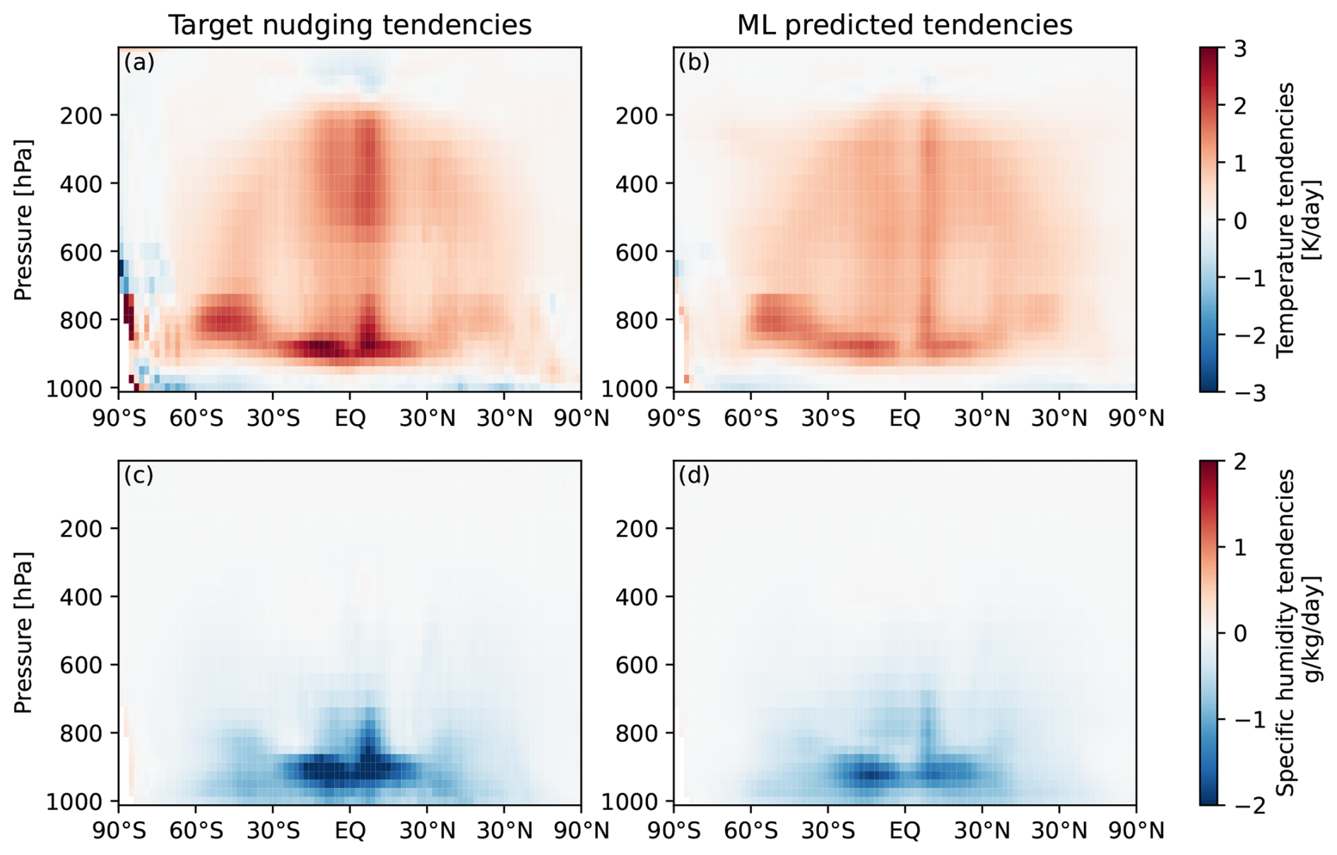
Figure 2 Zonal mean of target nudging tendencies (a, c) and ML-predicted tendencies (b, d) of air temperature and specific humidity over the 1-year free-running simulation.

While it is possible to avoid Python and instead directly interface with a trained ML model in C$++$ (e.g. via Tensorflow's C$++$ interface), our approach allowed us to take advantage of the existing fv3net package's robustness and stability. For example, we are able to take advantage of safeguards built into fv3net to ensure ML has physically-consistent output. Since fv3net is an end-to-end ML workflow, we also utilize its reporting for data analysis and visualization. Overall, using fv3net drastically reduced development time in every step of the ML workflow.

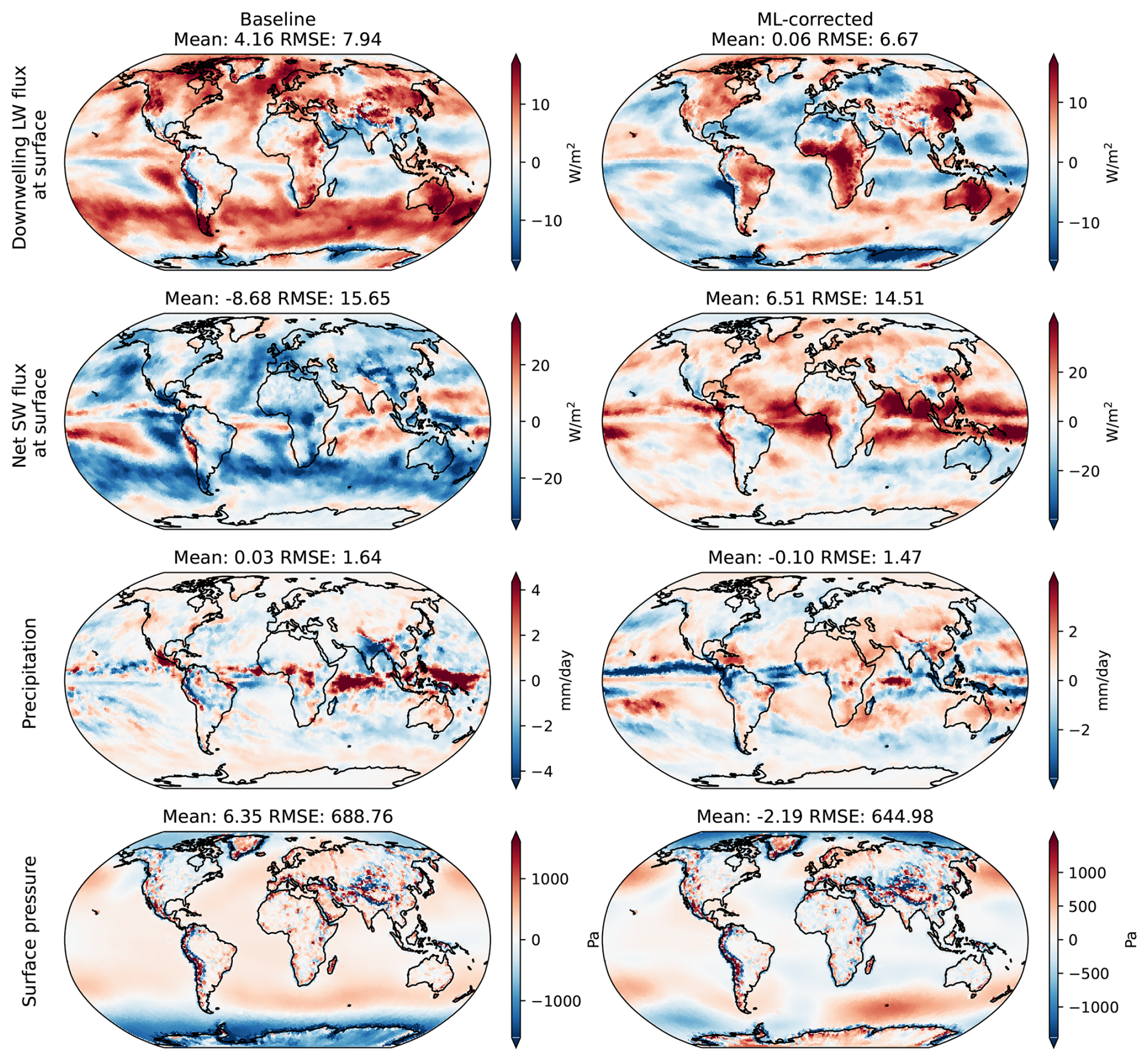
Figure 3 Spatial pattern of time mean simulation error with respect to the coarsened fine-grid reference simulation. Variables shown here, from top to bottom are the downwelling longwave flux and the net shortwave flux at the surface, the precipitation and the surface pressure. Shown here are the validation variables where the uncorrected coarse-resolution baseline (left column) has a higher RMSE than the coarse simulation including corrective-ML (right column). The RMSE is calculated as global area-weighted mean.

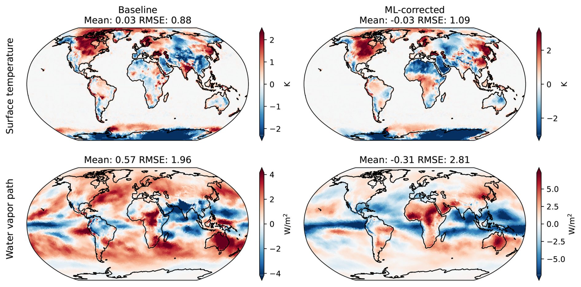
Figure 4 Same as Fig. 3, showing variables where the RMSE is worse for the ML-corrected simulation. These variables are the surface temperature (top) and the total integrated water vapor path (bottom).

4 Results from km-scale experiment

We present results from a 1-year free-running coarse-grid simulation that includes “online” ML correction toward the fine-grid reference (Donahue and Wu, 2025b). We use an uncorrected 100 km run as a baseline comparison. While the ML model captures the overall vertical structure of the target nudging tendencies for both temperature and specific humidity, it consistently underestimates the strength. This is illustrated in Fig. 2 for the temperature and specific humidity fields. Figures 3 and 4 show the annual-mean bias and root mean square error (RMSE) of baseline and ML-corrected runs from the reference data (3.25 km coarsened to 100 km, also used as ML training data). For this experiment, we found the largest improvement in surface downwelling longwave flux, with 16 % improvement in global RMSE when compared to the baseline. Additionally, we found marginal improvement (5 %–10 %) for net shortwave flux at the surface, precipitation, and surface pressure. However, RMSE was worse for surface temperature (24 %) and total water vapor path (43 %) in the ML-corrected run. Not shown are the eastward and northward wind comparisons, which showed little to no change between the nudged and ML-corrected solutions.

As shown in Fig. 2, the ML model exhibits its largest bias in the tropics. This underestimation of the target nudging tendencies likely contributes to the observed weakening of the ITCZ, because the model provides insufficient local heating and moistening to sustain the expected convergence and convective intensity. Recall that EAMxx currently does not include a deep convection scheme. This omission may help explain the greater weakening observed in the tropics, where stronger ML corrections would be required to reduce the bias.

The pattern of variables that improve or degrade is broadly consistent with the underestimation of nudging tendencies shown in Fig. 3. Surface radiative fluxes show the greatest improvement, which is plausible because the surface forcing model learns these fluxes directly from the fine-grid reference rather than inferring them from predicted tendencies. Precipitation and surface pressure improve more modestly. By contrast, water vapor path and surface temperature are closely linked to the temperature and specific humidity profiles that the model is designed to correct. When these corrections are systematically too weak, particularly in the tropics, as evident in Fig. 3, the ML-corrected simulation may become less self-consistent than the uncorrected baseline, leading to larger annual-mean errors in these fields.

To evaluate the stability and robustness of the corrective-ML approach, we conducted a series of training experiments using three different random seeds in the neural networks. During the online prognostic runs, models trained with seeds 1 and 3 crashed due to the inputs being out-of-sample. To address this issue, we adopted the method outlined in Sanford et al. (2023), training a separate out-of-sample novelty detector to complement the existing neural networks for temperature and specific humidity modeling. This approach proved reliable, allowing all random seeds to successfully complete a full-year simulation. We found the ML-predicted tendencies to be similar across random seeds, although these results are not shown.

5 Discussion

This study investigated the transferability of an ML parameterization from one GCM to another, a subject of growing importance as modeling groups plan to integrate ML machinery from other groups. Although we adopted the same strategy as Ai2, it quickly became clear that applying the workflow to a different atmospheric model would be challenging because of differences in GCM design and implementation. Each step in the corrective-ML workflow – nudging from coarse to fine-resolution simulation, prescribing surface fluxes for the coarse simulation, integrating ML, and diagnostics – is tightly coupled to the specifics of the underlying GCM, making generalization difficult. Even though this project was a collaboration between the team that developed EAMxx and the team that successfully applied this corrective-ML approach to FV3GFS, the end result fell short of the desired improvement from corrective-ML.

There are several possibilities for why corrective-ML was less successful for EAMxx than it was for FV3GFS. The most obvious difference between the two modeling frameworks is that the ML-corrected version of EAMxx does not include a deep convective parameterization and therefore produces a less realistic large-scale state. As a result, more is being asked of corrective-ML in EAMxx than in FV3GFS. Our initial expectation was that larger differences between the nudged and free-running low-resolution simulations would provide a stronger signal for training the ML. But in such an environment, imperfections in the corrective-ML will also stand out more. Potential improvements in the ML model from the stronger signal may be too small to offset the larger biases in EAMxx associated with the absence of a subgrid convection scheme. Additionally, this study was limited to 3-hourly averaged fields, rather than the instantaneous fields used in the FV3GFS study. Training on these smoother averaged fields may have reduced the ML model's skill in predicting the appropriate nudging tendencies for instantaneous states. Future work will address these hypotheses when EAMxx is enhanced to support a low-resolution configuration with parameterized deep convection.

As discussed in the Methods section, there are three independent ML models that make up the full corrective-ML implementation, each with its own set of parameters to train on. In this study, we focused on training the models following the same approach as with the FV3GFS test case (Bretherton et al., 2022). Given the differences between EAMxx and FV3GFS, it is possible that a successfully trained model may require an adjustment to the training hyperparameters. An example is the use of latitude as an input into the ML training data set. We found that the inclusion of latitude in the training input improved model accuracy, presumably as a proxy for physical variables that correlate strongly with latitude but are not well represented in the coarse GCM. A subsequent study could investigate what other parameters and input variables improve the performance of the ML models.

Adoption of the corrective-ML framework involved the development of several new features in EAMxx (https://github.com/E3SM-Project/E3SM, last access: 24 June 2024). EAMxx is heavily unit tested, but there is always a chance that a difficult bug or untested edge case is able to make it past the testing. There are three major developments that were added to EAMxx as part of this effort; Python to C$++$ bridging for ML, ability to nudge the EAMxx model state, and prescribed atmospheric surface fluxes in EAMxx. While significant effort went into developing and testing these new features, future work may want to revisit their implementation as a potential source of error in the ML implementation.

Finally, as outlined in the Methods section, the fine-resolution solution was coarsened to the target resolution both horizontally and vertically. The decision to map onto fixed vertical pressure coordinates resulted in situations where grid points over topography could lead to many or all data points being masked. This could create either masked data in the target state or grid points with disproportionate weighting based on only a few source columns. To investigate this hypothesis, a separate lightweight study was conducted using a 25 km fine-resolution simulation, comparing two corrective-ML models. One model utilized the approach described in this study, while the other did not apply vertical interpolation for the target state. Preliminary analysis showed that the latter model had slightly better performance. Unfortunately, due to the high cost of 3.25 km simulations, it was not feasible within the scope of this project to repeat this study using horizontal-only interpolation. A more detailed investigation of the impact from vertical interpolation should be included in any subsequent studies.

6 Conclusions

Although this work did not achieve the anticipated accuracy improvements from corrective-ML in EAMxx (Donahue et al., 2024), it did have several beneficial effects. In particular, this study marked the first time Python packages were integrated into EAMxx, providing a blueprint for future hybrid ML without degrading EAMxx performance on either CPU or GPU architectures. This work also led to the development of new infrastructure within EAMxx to support prescribed surface fluxes and atmospheric state nudging. While the latter was already a planned milestone for the regionally-refined configuration of EAMxx, this effort expanded that capability. The introduction of prescribed surface fluxes is important for some doubly-periodic use cases and useful for debugging and hypothesis testing (Bogenschutz et al., 2025). Finally, the fact that EAMxx benefited less from corrective-ML than FV3GFS (Bretherton et al., 2022) is a useful data point in the quest to understand generalizability of ML approaches in GCMs.

There is increasing interest in the earth system modeling community in utilizing differentiable algorithms and software. This strategy has already been successfully applied to NeuralGCM, which marries a spectral dycore coded in the Jax machine learning language with a learned ML representation of the combined physical parameterizations of a global model, trained to evolve following a gridded reanalysis. In this setting, the ML model can be trained end-to-end including feedbacks with other earth system components within this differentiable framework, dramatically improving the prognostic performance of this hybrid model such that it has highly accurate weather forecasts and strong climate skill (Kochkov et al., 2024). In principle, an analogous approach could be implemented to dramatically improve the prognostic skill of corrective-ML within EAMxx. However, refactoring EAMxx to enable such a capability while retaining leadership-class performance would be a substantial software engineering challenge.