Spatialize v1.0: a Python/C+ +  library for ensemble spatial interpolation

In this paper, we present Spatialize, an open-source library that implements ensemble spatial interpolation, a novel method that combines the simplicity of basic interpolation methods with the power of classical geostatistical tools, like Kriging. It leverages the richness of stochastic modelling and ensemble learning, making it robust, scalable and suitable for large datasets. In addition, Spatialize provides a powerful framework for uncertainty quantification, offering both point estimates and empirical posterior distributions. It is implemented in Python 3.x, with a C$++$ core for improved performance, and is designed to be easy to use, requiring minimal user intervention. This library aims to bridge the gap between expert and non-expert users of geostatistics by providing automated tools that rival traditional geostatistical methods. Here, we present a detailed description of Spatialize along with a wealth of examples of its use.

1 Introduction

A significant challenge in the field of geosciences is the issue of sparsity that is often observed in spatial databases, such as soil properties, climate data, or mineral concentrations, which are characterised at limited point locations (Li and Heap, 2014). The presence of these data gaps hinders a comprehensive understanding of the variable's domain. The central issue, therefore, is estimating values at unmeasured locations. Various spatial interpolation algorithms have been developed for this purpose.

Geostatistics is a field focused on the analysis, estimation, and modelling of spatial variables. Unlike traditional statistics, geostatistics emphasises the spatial dependencies between observations (Maroufpoor et al., 2020). The Kriging technique, the most relevant exponent of geostatistical interpolation (McKinley and Atkinson, 2020; Kirkwood et al., 2022), was initially devised for the estimation of gold reserves (Kleijnen, 2017; Virdee and Kottegoda, 1984). As an unbiased linear estimator that minimises estimation error at each position, Kriging is commonly referred to as BLUE (Best Linear Unbiased Estimator) (McKinley and Atkinson, 2020; Fischer and Getis, 2009; Varouchakis et al., 2012; Abzalov, 2016). Beyond providing robust estimates, Kriging also facilitates the calculation of estimation variance, which is widely used for assessing spatial prediction uncertainty (Abzalov, 2016; Varouchakis et al., 2012). A variety of user-friendly tools are available for the implementation of Kriging, including PyKrige (last access: 28 May 2026), PySAL (last access: 28 May 2026), gstat (last access: 28 May 2026), automap (last access: 28 May 2026), geoR (last access: 28 May 2026), and fields (last access: 28 May 2026). Nevertheless, it should be noted that the use of Kriging without actual knowledge of the model may result in suboptimal and misleading outcomes (Oliver and Webster, 2014; Assibey-Bonsu, 2017). In particular, parameter selection and spatial continuity modelling have a significant effect on the accuracy of Kriging estimates (Abzalov, 2016; Chilès and Desassis, 2018; Pannecoucke et al., 2020). However, the correct determination of these inputs requires substantial expertise and data (Fischer and Getis, 2009; Wang et al., 2017; Pannecoucke et al., 2020; de Sousa Mendes et al., 2020), which creates a significant barrier for most potential users. Moreover, the task becomes increasingly complex when the variables under study are of a dynamic, spatio-temporal nature (Samson and Deutsch, 2022; Boroh et al., 2022), or are not structurable as a regular grid (Oliver and Webster, 2014).

In summary, spatial interpolation tasks, when assessed from the perspective of classical geostatistical analysis, can be time-consuming and require considerable expertise. Consequently, there is a need for more straightforward yet effective spatial interpolation methods that can address highly dynamic spatial problems without necessitating manual spatial analysis tasks.

In contrast to geostatistical approaches, deterministic models employ straightforward calculations; nevertheless, they are only capable of producing estimations (Li and Heap, 2014), and thus do not offer uncertainty quantifications. The most widely applied of these methods is inverse distance weighting (IDW), a simple yet powerful spatial interpolation method that uses a weighted average of surrounding point values to estimate the unknown value at an unsampled location (Mitáš and Mitášová, 1988). In recent years, variants of IDW have been successfully used in a variety of applications, including estimation of air pollution levels (Li et al., 2017), soil moisture (Abdulwadood et al., 2021) and water quality (Khouni et al., 2021). The main limitation of IDW is that it does not take into account the spatial structure or correlation of the variable being interpolated. This can lead to over-smoothing or under-smoothing of the estimated values, depending on the degree of spatial correlation in the data (Li, 2021).

Another promising approach for spatial interpolation is the use of machine learning-based methods, which can learn complex spatial relationships from large datasets without requiring manual spatial modelling (Li et al., 2011; Kirkwood et al., 2022). For example, Leirvik and Yuan (2021) and Wang et al. (2019) proposed deep learning-based spatial interpolation methods to estimate solar radiation and interpolate seismic data, respectively. Nevertheless, challenges that arise from deep learning models are, firstly, the need for large amounts of data and computational resources to train them, and secondly, the necessity to measure additional variables other than the one under study. This is especially true for complex spatial-temporal problems, where the number of input variables and temporal observations can be substantial (Hamdi et al., 2022). A further challenge in using deep learning for spatial interpolation is the difficulty of interpreting the results. These models are often referred to as “black boxes”, meaning that the process by which predictions are derived remains uncertain. This can be problematic in situations where transparency and interpretability are important, such as in environmental applications (Paudel et al., 2023; Meng et al., 2013; Susanto et al., 2016).

In addressing the need for a simple and flexible spatial interpolation technique, able to adapt to highly dynamic phenomena, scalable to big data, interpretable, and most importantly widely accessible to the entire geoscientific community, Menafoglio et al. (2018) and Egaña et al. (2021) independently proposed a new state-of-the-art spatial interpolation method based on ensemble learning. This method combines the simplicity of methods such as IDW with the power of Kriging spatial analysis, which the authors of the latter named Ensemble Spatial Interpolation (ESI). This model is able to provide reliable estimates that are comparable to those of Kriging, while eliminating the need for manual spatial continuity modelling. Its main features are: (a) it is based on a stochastic space partitioning process, which aids in managing large datasets; (b) it is built under an ensemble scheme, which guarantees robustness despite the use of weak local interpolation functions with small subsets of data, and (c) it provides a powerful framework for uncertainty quantification, as it is based on a Bayesian scheme, thus yielding an empirical posterior distribution of the estimate (instead of a single point estimate).

The aim of this article is to present spatialize, a novel software library that facilitates an efficient implementation of ESI. Spatialize has been designed to be easy to use, efficient and flexible. The core of the library is implemented in C$++$ with a Python 3.x programming API. It is available as an open-source project, making it accessible to researchers and practitioners in industry and academia. The subsequent sections provide a comprehensive overview of the ESI model and the Spatialize library, including its features and capabilities. We also present several examples of how the library can be used in practical applications. Finally, the future directions of the library and its potential impact on spatial interpolation research and practice will be discussed.

2 Ensemble spatial interpolation

Ensemble learning is usually regarded as the statistical and computational conception of the “wisdom of the crowd”, whose idea is to collect and combine the points of view of many experts to produce an ensemble result (Egaña et al., 2021). An ensemble model $\widehat{z}$ can be formulated as:

$$\begin{array}{}\text{(1)}& \widehat{z}=G\left(f_{\mathrm{1}}\right({\mathit{x}}^{\ast }),\mathrm{\dots },f_m({\mathit{x}}^{\ast }\left)\right)\end{array}$$

where x^∗ is a vector of covariances and $\mathit{\{}{f}_{\mathrm{1}},\mathrm{\dots },f_m\mathit{\}}$ is a set of weak voter (regression, classification, interpolation, etc.) functions. Function G is an aggregation function that combines the responses from each voter function and it can be as simple as majority voting for classification (Friedman et al., 2000; Collins et al., 2002; Džeroski and Ženko, 2004; Hothorn and Lausen, 2005; Reid and Grudic, 2009), averaging for regression, or more sophisticated approaches such as a mixture of experts (MoE) (Jacobs et al., 1991; Jacobs, 1995; Jordan and Xu, 1995; Cohen and Intrator, 2000).

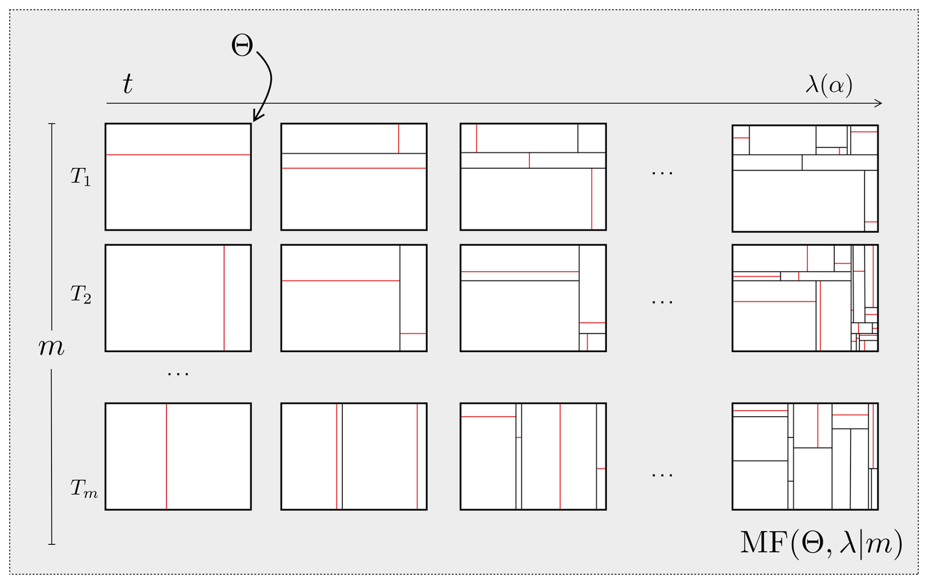
Figure 1 Generative process to draw a time-dependent stochastic partition set of size m. Time goes along the x-axis, ending at time given by λ(α), where α controls the average depth for the trees in the forest. Red lines indicate the current time partition cut. Note: Reprinted from “Ensemble Spatial Interpolation: A New Approach to Natural or Anthropogenic Variable Assessment”, by Egaña et al. (2021), Natural Resources Research, 30, 3777–3793.

2.1 Weak voter function set generation

In the ESI model, the construction of the set of weak voter functions is achieved through the concept of “bootstrapping the space” (Egaña et al., 2021), which involves generating different spatial configurations through random partitioning of the space where the data are located. These partitions are generated in a way that any combination of data is possible, while preserving their spatial locations and avoiding data clustering (Fig. 1). Each partition creates unique data subsets within the partition cells, where any spatial interpolation method can be applied. An unmeasured location is then estimated by combining (aggregating) the estimates derived from all the partition elements across the set of partitions where that location falls (Egaña et al., 2021).

It is well known that a spatial partition data structure can be represented as a tree (Samet, 1984), where nodes represent partition spaces and edges indicate containment relationships. This representation enables efficient spatial data querying and operations on the data contained in the spaces, similar to how certain related hierarchical data structures, such as k-d trees and octrees, are used in spatial indexing. Thus, in practice, generating a set of random partitions is equivalent to generating a forest of random tree structures, analogous to how multiple decision trees form a random forest.

The spatialize library uses two methodologies to generate these partitions of space:

(a) Mondrian Forests (MF): As proposed by Egaña et al. (2021) and introduced by Lakshminarayanan et al. (2014). The latter is a non-parametric Bayesian strategy that is employed for both classification and online regression, which has been demonstrated to be as efficacious as other high-level ensemble learning methods, such as random forests (Breiman, 2001) or additive trees (Hastie et al., 2009).

In the context of ESI, MF is a collection of random tree structures defined as:

$$\begin{array}{}\text{(2)}& \text{MF}(\mathrm{\Theta },\mathit{\lambda }|m)=\mathit{\{}{T}_{\mathrm{1}},\mathrm{\dots },T_m\mathit{\}},T_k\sim \text{MT}(\mathrm{\Theta },\mathit{\lambda })\end{array}$$

where m is the number of random tree structures in the forest and MT(Θ,λ) is the generative process, described in Algorithm 1, which produces random samples of tree structures. The latter represents random space partitions of the target domain Θ that are assumed to be $\mathrm{\Theta }=[a_{\mathrm{1}},b_{\mathrm{1}}]\times \mathrm{\dots }\times [a_d,b_d]\subset {\mathbb{R}}^d$.

Algorithm 1 MT(Θ,λ) Sampling Algorithm

1:

procedure Main()

2:

SampleMT(Θ,λ) {$\mathrm{\Theta }=[a_{\mathrm{1}},b_{\mathrm{1}}]\times \mathrm{\dots }\times [a_d,b_d]$}

3:

end procedure

4:

procedure SampleMT(θ,λ)

5:

SampleMTBranch($\mathit{\theta },\mathit{\lambda },\mathrm{0}$)

6:

end procedure

7:

procedure SampleMTBranch($\mathit{\theta },\mathit{\lambda },\mathit{\tau }$)

8:

E∼Exp(μ(θ)) {μ is a measure on ℝ^d}

9:

if $(\mathit{\tau }+E)<\mathit{\lambda }$ then

10:

$d_x\sim \text{Discrete}(p_{\mathrm{1}},\mathrm{\dots },p_d)$

11:

$x\sim U\left(\right[a_{d_x},b_{d_x}\left]\right)$

12:

SampleMTBranch(${\mathit{\theta }}^{>},\mathit{\lambda },(\mathit{\tau }+E)$)

13:

SampleMTBranch(${\mathit{\theta }}^{<},\mathit{\lambda },(\mathit{\tau }+E)$)

14:

end if

15:

end procedure

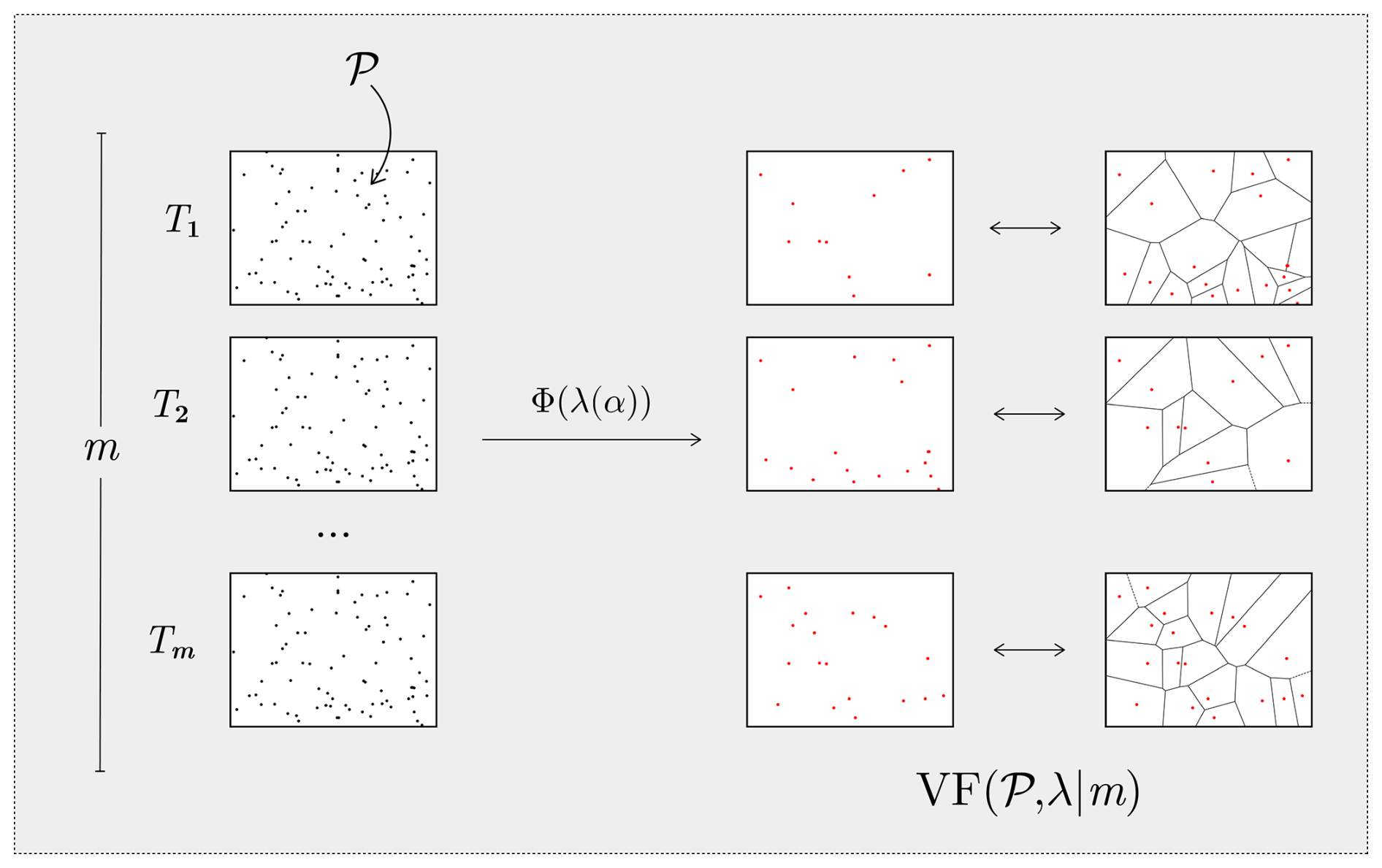
Figure 2 Generative process to draw a topological stochastic partition set of size m. The number of Voronoi nuclei is given by λ(α), where α controls the average depth for the partitions in the forest. Red points indicate the selected locations, among the sampled locations, for the nuclei.

Algorithm 1 implements a temporal stochastic process that generates Mondrian partitions, i.e. nested random partitions aligned with coordinate axes. Parameter λ represents the process's finite lifetime, while τ represents the elapsed time through recursion levels. The recursive partitioning process is as follows: Line 8 samples the “time” until the next cut in the sub-box θ from an exponential distribution, parametrized such that $\mathbb{E}\left(E\right)=\mathrm{1}/\mathit{\mu }\left(\mathit{\theta }\right)$, where $\mathit{\mu }\left(\mathit{\theta }\right)={\sum }_{i=\mathrm{1}}^d(b_i^{\mathit{\theta }}-a_i^{\mathit{\theta }})$. This ensures smaller sub-boxes are less likely to be partitioned. In line 10, the dimension to be partitioned is selected, where p_k determines the probability of selecting dimension k. For a sub-box θ, p_k is proportional to $(b_k^{\mathit{\theta }}-a_k^{\mathit{\theta }})$, favouring the partition of larger sides. In line 11, the cut point is randomly determined along the selected dimension, creating sub-boxes θ^> and θ^<. Figure 1 illustrates the partitioning process, with each red line representing a cut at time t for all T_k.

(b) Voronoi Forests (VF): A variation of (a) which employs Voronoi partitions instead of Mondrian trees, in a manner analogous to that described by Menafoglio et al. (2018). However, rather than using a fixed number of nuclei, spatialize employs a random number per partition, calibrated to ensure that the expected number of data points per cell matches that of a Mondrian tree.

Thus, a Voronoi Forest (VF) is a collection of structures defined as:

$$\begin{array}{}\text{(3)}& \text{VF}(\mathrm{\Theta },\mathit{\lambda }|m)=\mathit{\{}{T}_{\mathrm{1}},\mathrm{\dots },T_m\mathit{\}},T_k\sim \text{VT}(\mathrm{\Theta },\mathit{\lambda })\end{array}$$

where VT(Θ,λ) is the generative process that produces a Voronoi partition. The process begins with the selection of K, the number of Voronoi nuclei, which is drawn from a Poisson distribution with parameter λ. Next, a random sample of K nuclei, denoted by ${\mathrm{\Phi }}_K=\mathit{\{}{c}_{\mathrm{1}},\mathrm{\dots },c_K\mathit{\}}\subseteq \mathrm{\Theta }$, is randomly generated. Finally, the target domain Θ is partitioned by assigning all contained locations x∈Θ to the nearest nuclei based on the Euclidean distance. A Voronoi cell is thus defined by ${\mathcal{L}}_i=\mathit{\{}x\in \mathrm{\Theta }:\Vert x-c_i\Vert \le \Vert x-c_j\Vert \forall c_j\in {\mathrm{\Phi }}_K,j\ne i\mathit{\}}$. The process of generating a Voronoi Forest is illustrated in Fig. 2.

2.1.1 Model training

Let us define conditioning data as a set $\mathcal{M}=\mathit{\{}{z}_j{\mathit{\}}}_{j=\mathrm{1}}^{N_s}$ of N_s measurements of a variable of interest, obtained at specific spatial locations $\mathcal{P}=\mathit{\{}{\mathbf{\text{x}}}_j{\mathit{\}}}_{j=\mathrm{1}}^{N_s}$ within a particular region of a d-dimensional space. The classical formulation of spatial interpolation can be stated as: find a d-variate function S_(𝒫,ℳ) that fulfils the condition ${\mathbf{\text{S}}}_{(\mathcal{P},\mathcal{M})}\left({\mathbf{\text{x}}}_j\right)=z_j$, $j=\mathit{\{}\mathrm{1},\mathrm{\dots },N_s\mathit{\}}$¹.

Now, let us assume 𝒫⊂Θ. Then, both a Mondrian Forest, $\text{MF}(\mathrm{\Theta },\mathit{\lambda }|m)$, and a Voronoi Forest, $\text{VF}(\mathrm{\Theta },\mathit{\lambda }|m)$, can be “trained” when a set of d-dimensional data points (the conditioning data) are used to condition the sampling of $\mathit{\{}{T}_{\mathrm{1}},\mathrm{\dots },T_m\mathit{\}}$. We see, then, that:

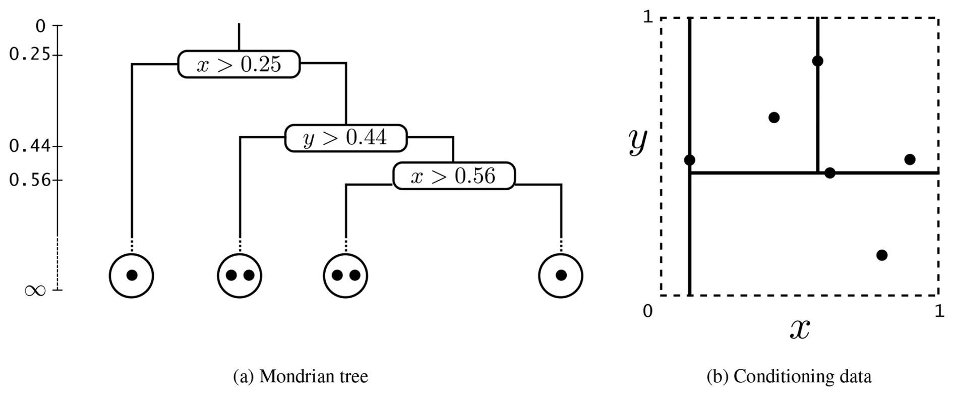
Figure 3 Tree structure schema. (a) Decision tree structure. (b) The spatial partition corresponding to the decision tree structure shown in (a). Black points represent conditioning data. Note: Reprinted from “Ensemble Spatial Interpolation: A New Approach to Natural or Anthropogenic Variable Assessment”, by Egaña et al. (2021), Natural Resources Research, 30, 3777–3793.

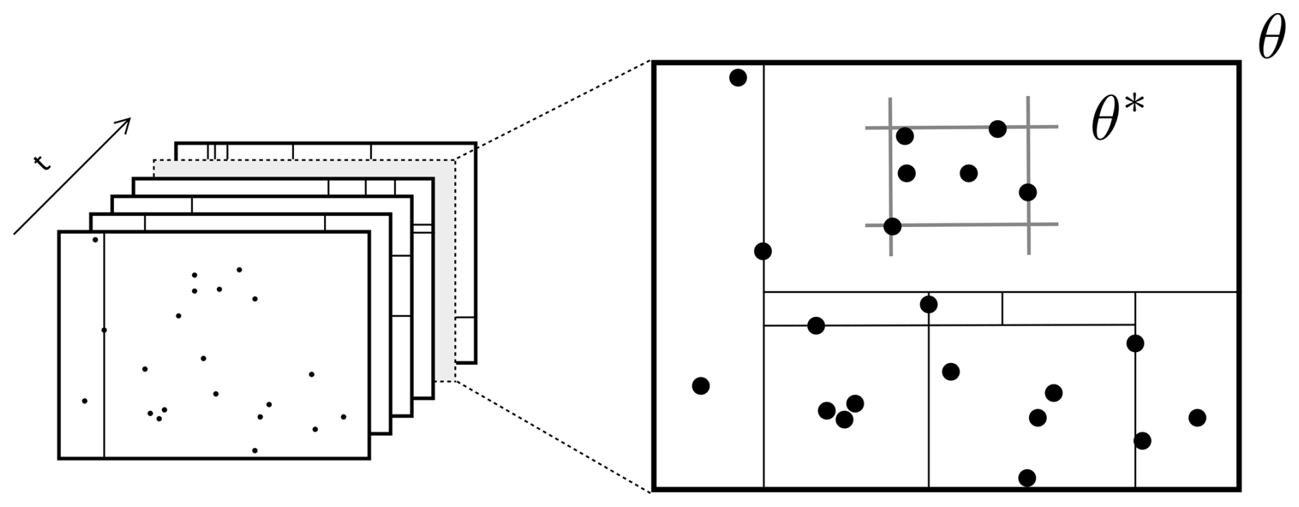
Figure 4 Illustration of θ^∗ given a set of data points, which enables Algorithm 1 to be trained using sample data. Note: Reprinted from “Ensemble Spatial Interpolation: A New Approach to Natural or Anthropogenic Variable Assessment”, by Egaña et al. (2021), Natural Resources Research, 30, 3777–3793.

(a) When using Mondrian Forests

A trained Mondrian Forest is defined as:

$$\begin{array}{}\text{(4)}& \text{MF}(\mathrm{\Theta },\mathit{\lambda }|\mathcal{P},m)=\mathit{\{}{T}_{\mathrm{1}},\mathrm{\dots },T_m\mathit{\}},T_k\sim \text{MT}(\mathrm{\Theta },\mathit{\lambda }\left|\mathcal{P}\right).\end{array}$$

A Mondrian tree can be trained by conditioning the partitioning process to the data (Fig. 3b). Thus, a trained random partition set, $\text{MF}(\mathrm{\Theta },\mathit{\lambda }|\mathcal{P},m)$, can be obtained by modifying Algorithm 1 as follows:

• For any box θ define ${\mathit{\theta }}^{\ast }=k(\mathit{\theta },\mathcal{P})$ as the smallest sub-box containing all conditioning positions in θ (see Fig. 4).

• The probability of splitting a sub-box (line 8) is replaced by: Sample $E\sim \text{Exp}\left(\mathit{\mu }\right({\mathit{\theta }}^{\ast }\left)\right)$.

• Lines 10 and 11 in Algorithm 1 are adjusted to work on θ^∗ instead of θ.

As a result of this modification, sub-boxes containing highly concentrated data are more likely to be partitioned. This offers the advantage of ensuring that most leaf nodes (i.e. the resulting sub-boxes) contain a reasonable amount of conditioning data, thus avoiding spatial clustering.

(b) When using Voronoi Forests

A trained Voronoi Forest (VF) is defined as:

$$\begin{array}{}\text{(5)}& \text{VF}(\mathrm{\Theta },\mathit{\lambda }|\mathcal{P},m)=\mathit{\{}{T}_{\mathrm{1}},\mathrm{\dots },T_m\mathit{\}},T_k\sim \text{VT}(\mathrm{\Theta },\mathit{\lambda }\left|\mathcal{P}\right).\end{array}$$

A trained random partition set, $\text{VF}(\mathrm{\Theta },\mathit{\lambda }|\mathcal{P},m)$, can be obtained by sampling the m sets of Voronoi nuclei from the locations at which measurements of the variable of interest are available, as opposed to being sampled from Θ. For each tree, this results in the set ${\mathrm{\Phi }}_K=\mathit{\{}{c}_{\mathrm{1}},\mathrm{\dots },c_K\mathit{\}}$ where K≤N_s and Φ_K⊆𝒫.

Thus, the process to obtain samples from $\text{VT}(\mathrm{\Theta },\mathit{\lambda }|\mathcal{P})$ is as follows:

• Sample $K\sim \text{Poisson}\left(\mathit{\lambda }\right),\mathrm{1}\le K\le N_s$.

• Sample ${\mathrm{\Phi }}_K=\mathit{\{}{c}_{\mathrm{1}},\mathrm{\dots },c_K\mathit{\}}$ from the measured locations 𝒫

• Establish each Voronoi cell as ${\mathcal{L}}_i=\mathit{\{}x\in \mathrm{\Theta }:\Vert x-c_i\Vert \le \Vert x-c_j\Vert \forall c_j\in {\mathrm{\Phi }}_K,j\ne i\mathit{\}}$.

Sampling from the measured locations 𝒫 ensures that all partition cells ${\mathcal{L}}_{\mathrm{1}},\mathrm{\dots },{\mathcal{L}}_K$, generated by sampling $\text{VT}(\mathrm{\Theta },\mathit{\lambda }|\mathcal{P})$, will contain at least one measured location.

2.1.2 Weak voter function set

For an unmeasured position ${\mathit{x}}^{\ast }\in \mathrm{\Theta }$, we define ${\mathcal{L}}_k\subset (\mathcal{P},\mathcal{M})$ as the set of conditioning data points contained within the partition cell where x^∗ falls into in tree T_k.

Then, let us consider a base interpolation function S_(𝒫,ℳ), which can be any spatial interpolator for which no additional information, other than measurements and their locations, is required to interpolate new positions – such as Kriging or IDW.

Now, for each tree T_k, let ${\mathbf{\text{S}}}_{{\mathcal{L}}_k}$ be the base interpolation function restricted to ℒ_k. Thus, the kth weak voter function for x^∗ is obtained by applying the base interpolator S_(𝒫,ℳ) to estimate the value at x^∗ using only the points in ℒ_k.

Formally, the weak voter function set is defined as:

$$\begin{array}{}\text{(6)}& f_k\left({\mathit{x}}^{\ast }\right)={\mathbf{\text{S}}}_{{\mathcal{L}}_k}\left({\mathit{x}}^{\ast }\right),k=\mathrm{1},\mathrm{\dots },m.\end{array}$$

2.2 Interpolation using the trained model

Let us denote $x_k^{\ast }=f_k\left({\mathit{x}}^{\ast }\right)={\mathbf{\text{S}}}_{{\mathcal{L}}_k}\left({\mathit{x}}^{\ast }\right)$ as the kth weak voter function for x^∗. Then, $\mathit{\{}{x}_k^{\ast }{\mathit{\}}}_{k=\mathrm{1}}^m$ corresponds to the set of weak voter functions for x^∗ resulting from all m trees.

Thus, the interpolation function 𝒵_(𝒫,ℳ) corresponds to the aggregation of these weak voter functions:

$$\begin{array}{}\text{(7)}& e^{\ast }={\mathcal{Z}}_{(\mathcal{P},\mathcal{M})}\left({\mathit{x}}^{\ast }\right)=G\left(\mathit{\{}{x}_k^{\ast }{\mathit{\}}}_{k=\mathrm{1}}^m\right).\end{array}$$

The simplest choice for the aggregation function G is the mean 𝔼[⋅]. In this case, the interpolation function becomes:

$$\begin{array}{}\text{(8)}& e_{\mathbb{E}}^{\ast }={\displaystyle \frac{\mathrm{1}}{m}}\sum _{k=\mathrm{1}}^m{x}_k^{\ast }.\end{array}$$

2.3 Interpolation precision modelling

A precision model p^∗ for ${\mathcal{Z}}_{(\mathcal{P},\mathcal{M})}\left({\mathit{x}}^{\ast }\right)$ can be defined using a loss function 𝕃 as follows:

$$\begin{array}{}\text{(9)}& p^{\ast }={\mathbb{E}}_{\widehat{P}\left(\mathit{\{}{x}_k^{\ast }{\mathit{\}}}_m\right)}\left(\mathbb{L}\left(e^{\ast },\mathit{\{}{x}_k^{\ast }{\mathit{\}}}_m\right)\right).\end{array}$$

Equation (9) represents a generalisation of the mean-variance concept within the context of Bayesian variability. Here, ${\mathbb{E}}_{\widehat{P}(\cdot )}$, represents the expectation over the posterior distribution, averages 𝕃 over all sampled partitions, weighted by their posterior probability.

When using the mean-based interpolator $e_{\mathbb{E}}^{\ast }$, we can define an associated interpolation variance (or error) ${\mathbb{V}}_{e_{\mathbb{E}}^{\ast }}\left({\mathit{x}}^{\ast }\right)$ as:

$$\begin{array}{}\text{(10)}& p_{\mathbb{E}}^{\ast }={\mathbb{V}}_{e_{\mathbb{E}}^{\ast }}\left({\mathit{x}}^{\ast }\right)={\displaystyle \frac{\mathrm{1}}{m}}\sum _{k=\mathrm{1}}^m{\left(x_k^{\ast }-e_{\mathbb{E}}^{\ast }\right)}^{\mathrm{2}}.\end{array}$$

2.4 Rule of thumb for parameter choice

2.4.1 When using Mondrian Forests

The domain parameter Θ can be considered as any bounding box containing the positions of the conditioning data 𝒫. Thus, in practice, the only two parameters of the model are:

• The number of partitions (or tree structures) m. A reasonable suggestion for this parameter is that higher is better, keeping in mind that higher values will directly impact time performance. Experiments have shown that certain stability is reached for m≥500 (Egaña et al., 2021), so this would be a good starting point.

• The process lifetime λ. The only restriction for this parameter is that it must be positive. This renders the selection, or any sensitivity analysis, of its value challenging. In order to address this issue, a function of a normalised parameter $\mathit{\alpha }\in [\mathrm{0},\mathrm{1})$ is used to obtain suitable values for λ, which is defined as follows:

  $$\begin{array}{}\text{(11)}& \mathit{\lambda }\left(\mathit{\alpha }\right)={\displaystyle \frac{\mathrm{1}}{\mathit{\mu }\left(\mathrm{\Theta }\right)(\mathrm{1}-\mathit{\alpha })}}.\end{array}$$

  In practice, α controls the average tree depth in the forest, determining how finely the space is partitioned. In this way, α=0 will generate the coarsest partition, while α→1 will generate finer ones. α must be carefully chosen to ensure that the base interpolation function ${\mathbf{\text{S}}}_{{\mathcal{L}}_k}$ has sufficient sample data. Once m has been defined, it is recommended to use cross-validation to find the optimal α, typically within [0.7,0.95].

2.4.2 When using Voronoi Forests

As seen in Mondrian Forest, the domain parameter Θ may be regarded as any bounding box encompassing 𝒫. Consequently, the parameters of the model remain identical, yet their respective roles and practical considerations differ:

• The number of partitions (or tree structures) m. A reasonable suggestion for this parameter is that higher is better, keeping in mind that higher values will directly impact time performance. However, the possibility of reaching stability for a certain value of m is yet to be studied in the context of Voronoi Forests.

• The process lifetime λ. This parameter determines the expected number of Voronoi nuclei for each partition. In the context of Voronoi Forest, λ is related to the mean of the Poisson distribution. Although the only theoretical restriction for this parameter is that it must be greater than one, in spatialize, it is also constrained to match the expected number of leaves in a Mondrian tree. To this end, λ is calculated by multiplying the parameter α, defined in the context of Mondrian forests, by a factor according to the number of observations N_s, as follows:

  $$\begin{array}{}\text{(12)}& \mathit{\lambda }\left(\mathit{\alpha }\right)={\displaystyle \frac{\mathrm{1}}{\mathrm{2}}}\times N_s\times \mathit{\alpha },\mathit{\alpha }\in [\mathrm{0},\mathrm{1}).\end{array}$$

  As in the case of Mondrian partitions, α also controls how coarse or fine the partitions are by affecting the number of Voronoi nuclei. Thus, α=0.25 will generate the coarsest partition, while α→1 will generate finer ones.

In the context of sampling from a trained tree $\text{VT}(\mathrm{\Theta },\mathit{\lambda }|\mathcal{P})$, additional considerations arise with respect to m and λ. Firstly, the number of nuclei, K(λ(α)), must not exceed the number of observations, N_s. Secondly, as K(λ(α))→N_s, when sampling from 𝒫, the number of possible Voronoi nuclei combinations decreases, and thus a large m value may result in duplicated partitions. To avoid such inefficiencies, it is recommended that $m\ll \left(\genfrac{}{}{0ex}{}{N_s}{K}\right)$, or alternatively, not employing trained trees (also possible on spatialize). Alternatively, spatialize also permits the direct sampling of Φ_K from Θ (i.e. not employing trained trees).

3 The spatialize library

Spatialize is an open source library for spatial analysis which offers different tools for implementing the Ensemble Spatial Interpolation (ESI) model. The main motivation behind the development of the spatialize library was to provide the scientific and technical community with a robust and automated spatial estimation tool that can be used across different disciplines by researchers and professionals who are not experts in geostatistics. In this sense, spatialize provides automated tools that eliminate the need for manual spatial analysis and extensive domain expertise.

The spatialize library is organized into three functional layers. First, the API is implemented in Python, offering three high-level functions: esi_griddata() performs ESI estimation on regular grids, esi_nongriddata() generates estimates at arbitrary spatial locations, and esi_hparams_search() searches for optimal ESI parameters. The latter employs cross-validation to determine the parameter combination that yields the minimum error out of a previously defined set. Second, the library provides aggregation functions according to Eq. (1), as well as precision estimation functions following Eq. (9), including a class for implementing custom precision functions. Test datasets are also included. Third, the spatial estimation methods are efficiently implemented in C$++$ for optimal performance.

The three main functions – esi_hparams_search(), esi_griddata(), and esi_nongriddata() – share three mandatory parameters: points, an n-samples × n-dimensions array specifying sample locations; values, an n-samples × 1 array containing the observed values at these locations; and xi, the query locations where estimates are required (as a standard array for non-gridded data or a meshgrid for gridded data). Optional arguments include ESI-specific parameters (n_partitions, alpha, data_cond, agg_function, seed, local_interpolator, and p_process) and local interpolator-specific parameters. A comprehensive description of these functions and their arguments can be found in the user manual, which is provided as supplementary material.

Spatialize 1.0.2 offers two alternatives for ESI local interpolators: Inverse Distance Weighting (IDW), a deterministic interpolator that assigns greater weighting to points in closer proximity, and an Ordinary Kriging variant with a normalized covariance matrix. Additionally, an implementation of traditional IDW is provided. In a different vein, two space partitioning methods are available, Mondrian Forests and Voronoi Forests².

Table 1 Comparison of spatialize with commonly used spatial interpolation libraries.

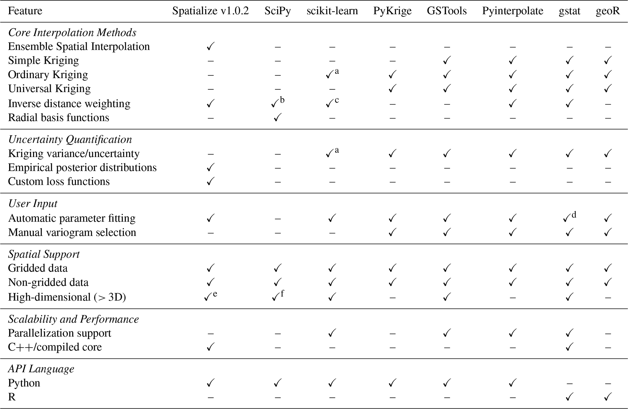
^a Through Gaussian Process Regression (GaussianProcessRegressor). ^b Must be manually implemented using (scipy.spatial.distance). ^c Through k-nearest neighbors (KNeighborsRegressor). ^d Available using automap. ^e Only available with Mondrian partitions. ^f RBFInterpolator supports arbitrary dimensions.

Table 1 offers a comparative analysis of the capabilities of spatialize and those of libraries commonly utilized for spatial interpolation.

The functionality of the aforementioned tools is demonstrated in the subsequent section.

4 Usage examples

The standard usage of spatialize follows a clear roadmap:

• 1.

  definition of inputs (points, values, xi);

• 2.

  hyperparameter optimization using the esi_hparams_search function;

• 3.

  execution of the ESI algorithm using either esi_griddata() or esi_nongriddata();

• 4.

  retrieving the estimation with result.estimation() and the uncertainty quantification with result.precision().

This section presents usage examples demonstrating the core functionality of spatialize, including hyperparameter optimization, gridded and non-gridded data estimation, and uncertainty quantification.

These examples illustrate how automated grid searches over ESI parameters make geostatistical spatial estimation accessible without requiring expert selection of a priori parameters, while achieving performance comparable to or better than other automatic spatial estimation tools, as well as offering uncertainty quantifications. For comparison, examples using SciPy and PyKrige are also presented.

4.1 Datasets

The examples are built upon two distinct case studies: a synthetic dataset and a real-world dataset.

4.1.1 Synthetic dataset

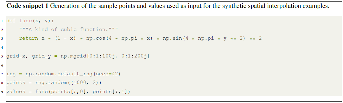
The synthetic dataset consists of a two-dimensional surface defined by a cubic-type function, adapted from the scipy.inter polate.griddata documentation. This function exhibits non-linear spatial variation with oscillatory features, making it suitable for evaluating interpolation performance under controlled conditions.

The dataset comprises a regular grid of 100 × 200 points spanning the unit square $[\mathrm{0},\mathrm{1}]\times [\mathrm{0},\mathrm{1}]$, with 1000 randomly sampled data points and ground truth values available at all grid locations.

The primary purpose of using synthetic data is to enable thorough quantitative performance evaluation by calculating error metrics (RMSE, MAE, etc.) across the entire estimation grid. This is not possible in real-world applications, where reference values are typically limited to sampled locations.

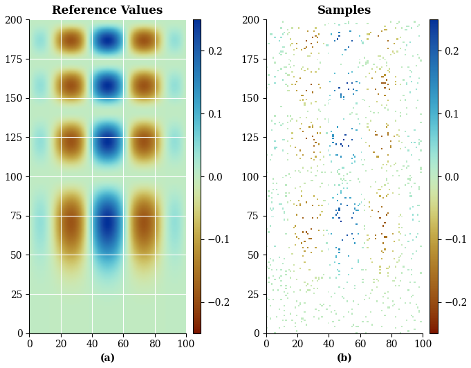
Figure 5 (a) Ground truth cubic function alongside (b) randomly sampled conditioning data (n=1000) used for spatial interpolation.

Code snippet 1 shows the generation of the grid, sampling points, and corresponding values generated by the cubic type function. Figure 5 illustrates the underlying function alongside the randomly sampled conditioning data used for interpolation.

In this case study, we evaluate spatialize performance on gridded estimation using the esi_griddata() function. We compare ESI implementations with IDW and Kriging as local interpolators (ESI-IDW and ESI-Kriging, respectively) against traditional IDW and SciPy interpolators. We employ the esi_hparams_search() function to automatically optimize ESI hyperparameters through grid search, demonstrating the library's capability for automated tuning without requiring expert knowledge. Additionally, we demonstrate the process of quantifying uncertainty through built-in and custom loss functions.

4.1.2 Real-world dataset

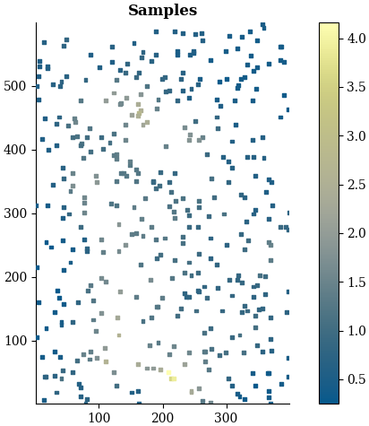
The real-world dataset consists of copper grade measurements from drill holes in the Andes, representing a typical mineral exploration scenario with sparse spatial sampling. The irregular sampling pattern reflects realistic exploration drilling strategies where sample locations are constrained by geological, topographical, and economic factors.

The dataset comprises 400 copper grade measurements at irregularly spaced locations over a $[\mathrm{0},\mathrm{400}]\times [\mathrm{0},\mathrm{600}]$ spatial extent. The estimation domain is discretized using a regular two-dimensional grid with uniform 2-unit spacing, resulting in 200 × 300 nodes for a total of 60 000 estimation points.

The dataset employed for this example, as well as corresponding Ordinary Kriging baseline estimates, are available directly through spatialize, as shown in Code snippet 2.

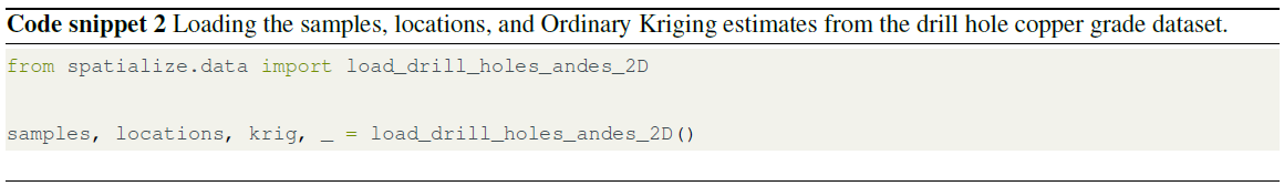
The available samples are displayed in Fig. 6.

Figure 6 Copper grade measurements used for spatial interpolation.

In this case study, we demonstrate spatialize performance on real-world non-gridded data using the esi_nongriddata() function. We compare ESI-IDW with different partitioning strategies (Mondrian and Voronoi) against ESI-Kriging and Ordinary Kriging. We assess performance via cross-validation, since ground truth values are unavailable at unsampled locations.

4.2 Synthetic data case study

This section presents the procedure and results from the synthetic data case study, demonstrating the use of spatialize on gridded data.

4.2.1 Spatialize: ESI-IDW implementation

We begin by implementing ESI with IDW as local interpolator.

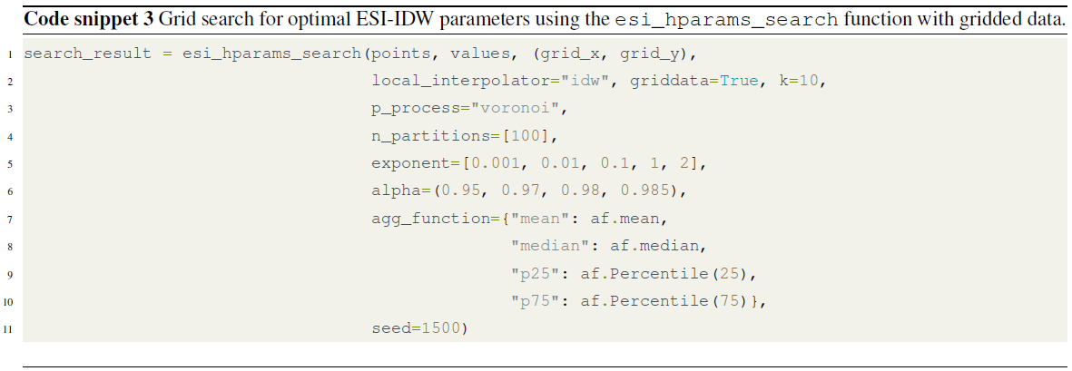
First, we perform a parameter search using the esi_hparams_search function. As shown in Code snippet 3, this function receives ranges or sets of parameters that produce different combinations for interpolation. We define a comprehensive set of combinations, including different exponent values, alpha values, and aggregation functions. Additionally, we use the Voronoi partitioning method because it generates more regular partition elements, which aligns well with the radial nature of the local IDW interpolator.

Since interpolation methods reproduce reference data values at grid points by construction, the parameter search function employs K-fold cross-validation to calculate the error. K points are removed from the dataset in each iteration, and the estimation error is calculated at these locations. The final error metric is obtained by averaging across all iterations. In this example, we use K=10.

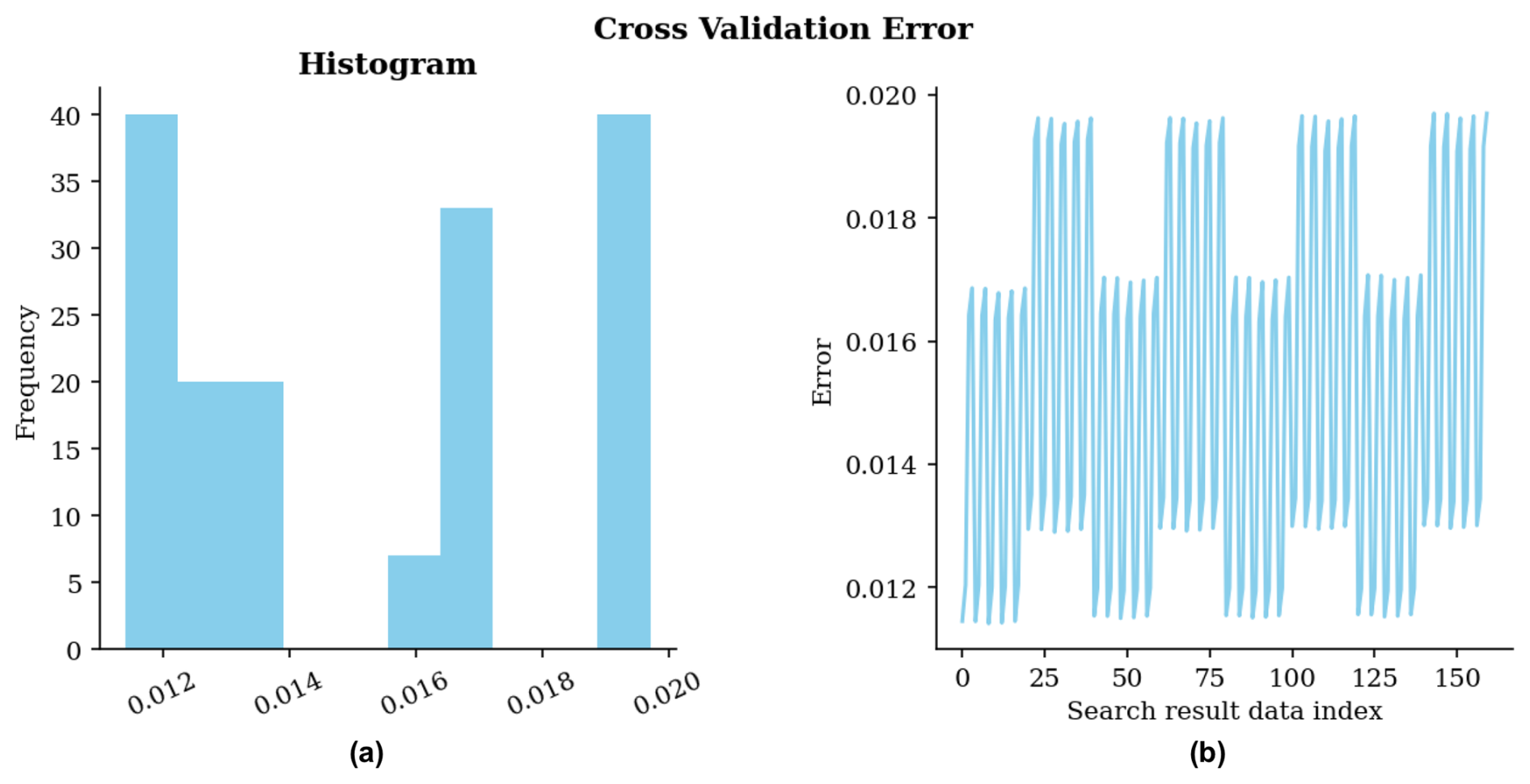
Figure 7 Cross-validation error for grid search using IDW as local interpolator. (a) Histogram of errors; (b) errors in the sequence of scenarios during the search.

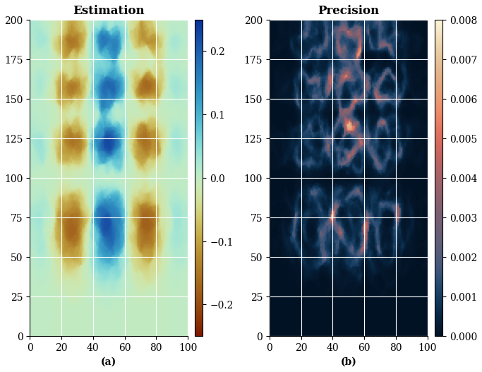
Figure 8 (a) ESI grid search best estimation using IDW as local interpolator; (b) Precision obtained with MSE (default) loss function.

In Code snippet 3, the object search_result stores the grid search results. Figure 7 displays the cross-validation errors for the 100+ parameter combinations evaluated during the search. The dual visualization provides complementary insights: the histogram (left panel) shows the distribution of estimation errors, while the sequential plot (right panel) reveals the evolution of error across scenarios. This plot can be quickly obtained using the method search_result.plot_cv_error().

The minimum error of 0.0114 was achieved in scenario number 8, which corresponds to the following parameters:

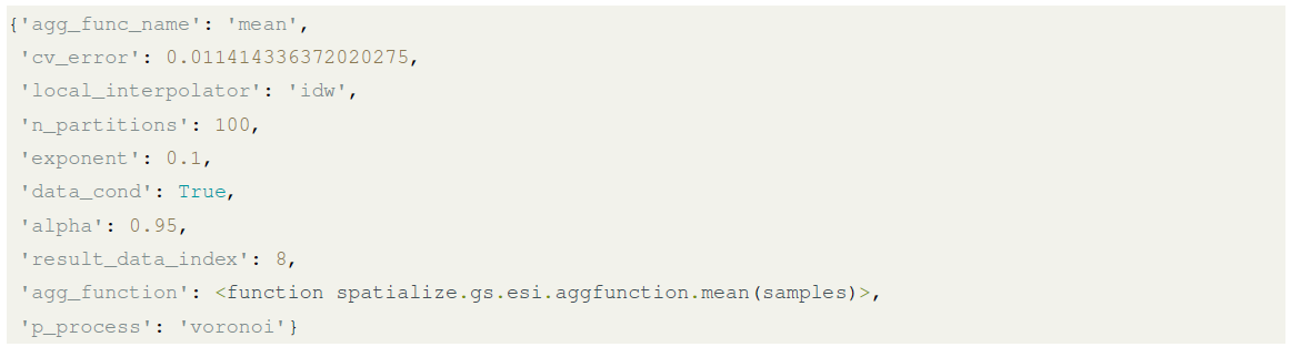
Finally, Code snippet 4 performs the ESI-IDW estimation using the optimal parameters found in the search. For convenience, the estimation function is designed to accept the dictionary returned by the method search_result.best_result() directly as an argument³. The estimates can be then retrieved using the result.estimation() method, while their corresponding precision is obtained through result.precision().

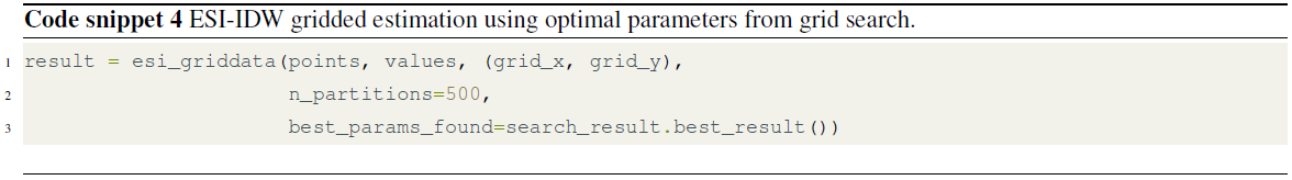
Figure 8 presents the ESI-IDW estimation alongside its corresponding precision map, calculated with the default loss function (MSE). The resulting interpolation partially captures the structural features of the reference function, though some differences remain, particularly in regions characterized by pronounced spatial variation. Accordingly, the precision map reveals elevated uncertainty in these same regions.

4.2.2 Spatialize: ESI-Kriging implementation

We now employ Kriging as the local interpolator for ESI, following the same parameter search and estimation procedure described in the ESI-IDW example. The underlying partitioning is carried out using the Mondrian forest process.

Code snippet 5 implements the parameter optimization process. We evaluate four omnidirectional variogram models across a range of nugget and sill values. The function generates and compares all possible parameter combinations to identify the optimal configuration.

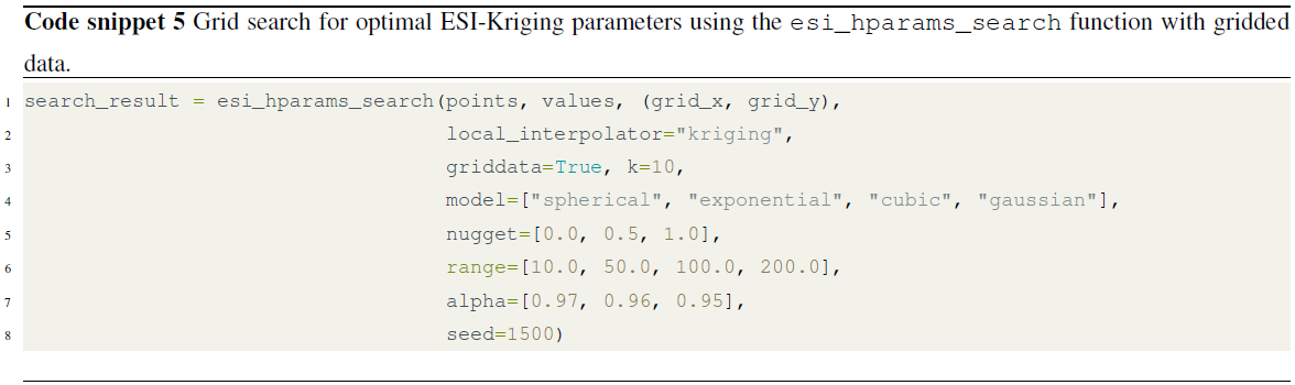
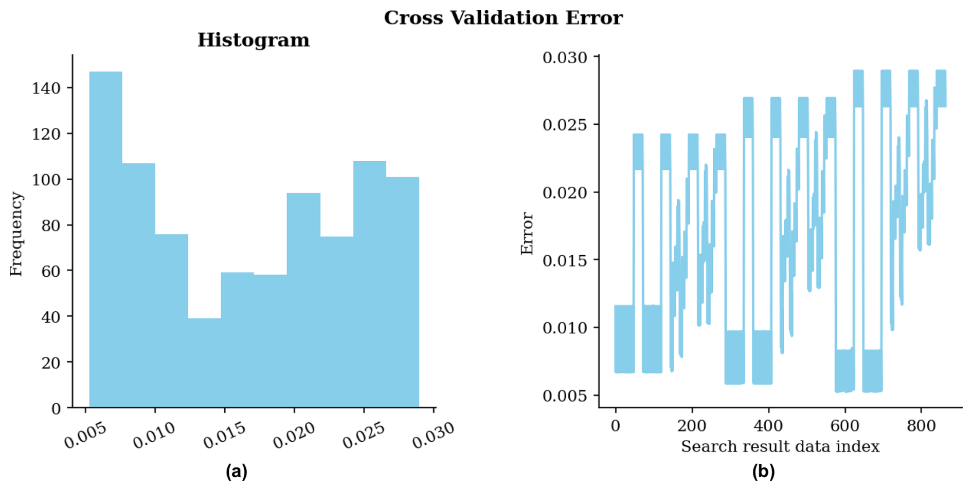
Figure 9 Cross-validation error for ESI grid search using Kriging as local interpolator. (a) Histogram of errors; (b) Errors in the sequence of scenarios during the search.

Figure 9 shows the cross-validation error frequency graphs (left) and the different error levels for each scenario (right).

Finally, we perform the estimation based on the parameters of the scenario with the lowest cross-validation error, which in this case has a value of 0.0053 at index 603. The optimal parameters are the following:

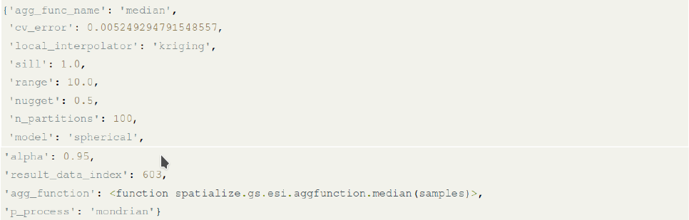
Code snippet 6 shows the implementation of ESI, applying the optimized parameters through the best_params_found argument. Just as in the ESI-IDW case, using result.estimation() returns the estimates, while result.precision() computes their precision.

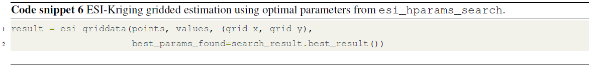
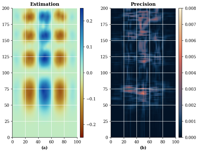
Figure 10 (a) ESI grid search best estimation using Kriging as local interpolator; (b) Precision obtained with MSE (default) loss function.

Figure 10 presents the ESI-Kriging estimation alongside its corresponding precision map, calculated with the default loss function (MSE). The ESI-Kriging interpolation successfully recovers the structural features of the reference function, despite the absence of domain-specific knowledge or formal variographic analysis in the model specification. The precision map reveals generally low uncertainty throughout the domain, with localized increases near boundaries of high-gradient regions, consistent with expected interpolation behaviour in areas of rapid spatial variation.

4.2.3 Spatialize: custom precision functions

In this section, we demonstrate the implementation of custom precision metrics for ESI estimates. As a reminder, precision in ESI is calculated by aggregating a loss function that compares each partition-specific ESI estimate with the final aggregated estimation.

The spatialize library provides a modular framework for implementing custom loss functions. For instance, Code Snippet 7 demonstrates a custom implementation of the operational error loss, which is also available as a built-in class in the lossfunction module.

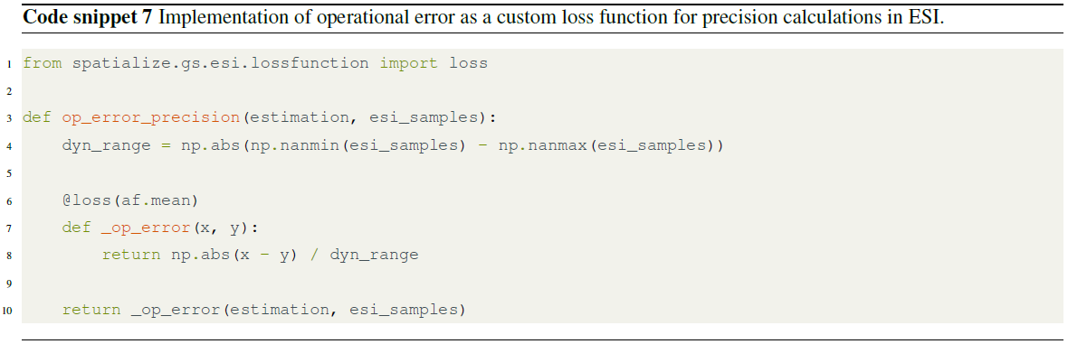
The function architecture consists of two nested components: an outer function that computes necessary parameters, and an inner function decorated with @loss() that specifies both the point-wise error calculation and the aggregation method for combining scenario-specific losses into a single precision layer. The operational error precision can then be obtained by using result.precision(op_error_precision).

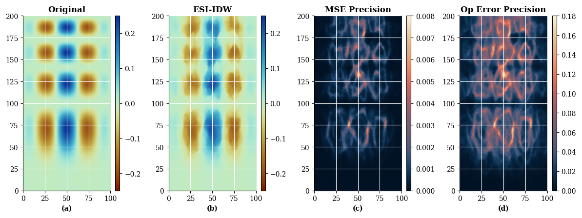
Figure 11 Mean squared error and operational error precision for an ESI-IDW interpolation. (a) The original cubic type function; (b) ESI-IDW interpolation; (c) Mean squared error precision; (d) Operational error precision.

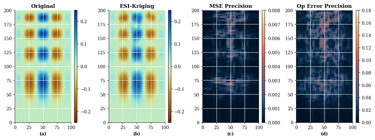
Figure 12 Mean squared error and operational error for an ESI-Kriging interpolation. (a) The original cubic type function; (b) ESI-Kriging interpolation; (c) Mean squared error precision; (d) Operational error precision.

Figures 11 and 12 compare the default MSE-based precision (contained in the ESIResult object) with the precision calculated using the custom operational error function for ESI-IDW and ESI-Kriging, respectively.

Both precision functions illustrate that ESI-IDW estimates have a higher uncertainty than those produced by ESI-Kriging in this scenario. However, each loss function highlights different aspects of this uncertainty. The mean squared error precision emphasizes regions of higher uncertainty, whereas the operational error precision clearly delineates the uncertainty in the spatial structure itself as represented by the interpolation.

4.2.4 Comparison with traditional IDW

To demonstrate the added value of ensemble spatial interpolation, we now compare the estimates provided by standard IDW interpolation against the previously presented ESI-IDW estimations.

First, Code snippet 8 implements an automated hyperparameter optimization using the idw_hparams_search function, analogous to the esi_hparams_search function.

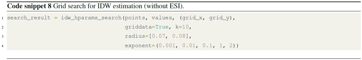
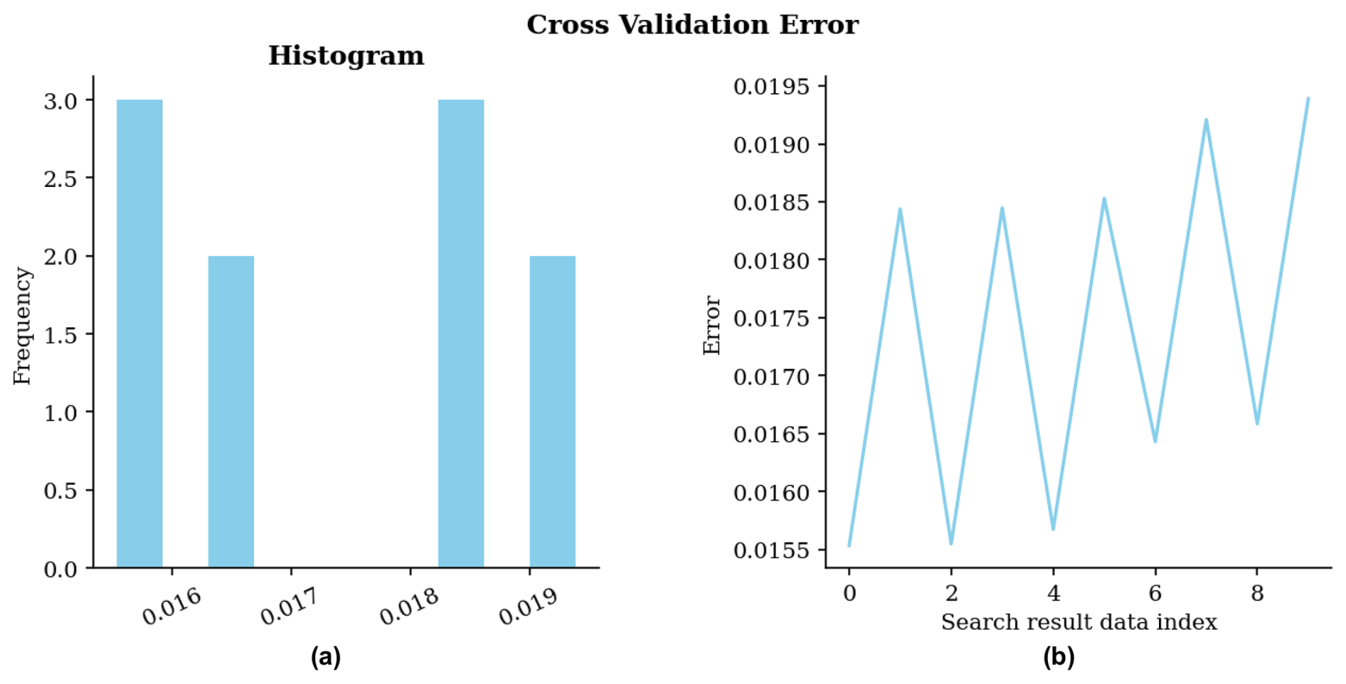
Figure 13 Cross-validation error for grid search for IDW interpolator without ESI. (a) Histogram of errors; (b) Errors in the sequence of scenarios during the search.

Figure 13 illustrates the cross-validation errors for each scenario in the grid search. The minimum error obtained has a value of 0.0155 at index 0. This scenario used a radius of 0.07 and an exponent of 0.001.

Then, we generate estimates using the best hyperparameters found in the search, as shown in Code snippet 9.

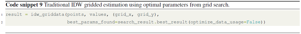
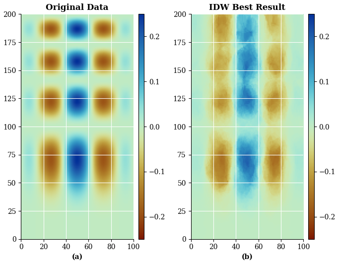
Figure 14 Best estimation using IDW interpolator without ESI. (a) The original cubic type function; (b) Traditional IDW interpolation.

Figure 14 shows the IDW estimates obtained using the optimal parameters. While the interpolator partially recovers the original image structures, ESI-IDW (Fig. 8) achieves notably superior resemblance to the reference image.

4.2.5 Comparison with SciPy

To benchmark our results against established Python interpolation tools, we employ the griddata function from the scipy.interpolate module using three standard methods: “nearest neighbour”, “linear” and “cubic” interpolation. Code snippet 10 demonstrates the implementation of these three approaches.

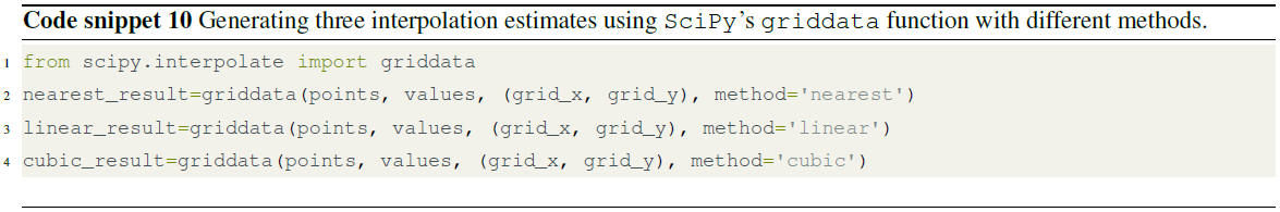
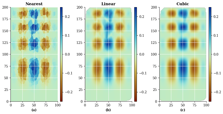
Figure 15 Comparison of SciPy estimates for the same gridded dataset. (a) Nearest-neighbour interpolation; (b) Linear interpolation; (c) Piecewise cubic interpolation.

Figure 15 presents the estimates generated by the three SciPy interpolation methods. Since the ground-truth function is cubic, the cubic interpolator unsurprisingly achieves the best visual reconstruction. This illustrates the inductive bias effect: when prior knowledge about the underlying function is available, selecting a matching interpolator yields superior results. However, in practical scenarios lacking such previous knowledge, choosing an appropriate interpolator becomes challenging.

Finally, it should be noted that the interpolators implemented in the SciPy library are deterministic and therefore do not provide uncertainty quantification.

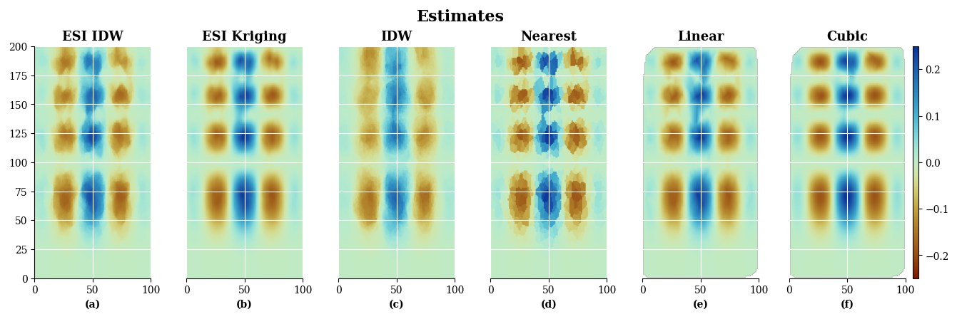
Figure 16 Comparison of ESI and SciPy estimates for the same gridded dataset. (a) ESI-IDW interpolation; (b) ESI-Kriging interpolation; (c) IDW interpolation; (d) SciPy nearest-neighbour interpolation; (e) SciPy linear interpolation; (f) SciPy piecewise cubic interpolation.

4.2.6 Performance comparison

This section provides a visual and quantitative comparison of all interpolators employed in the synthetic data case study.

Figure 16 presents the estimates side-by-side. Visually, ESI Kriging, along with the linear and cubic interpolators, appear to offer the best reconstruction of the target image. Notably, ESI achieves acceptable results without prior structural assumptions, as opposed to the SciPy interpolators.

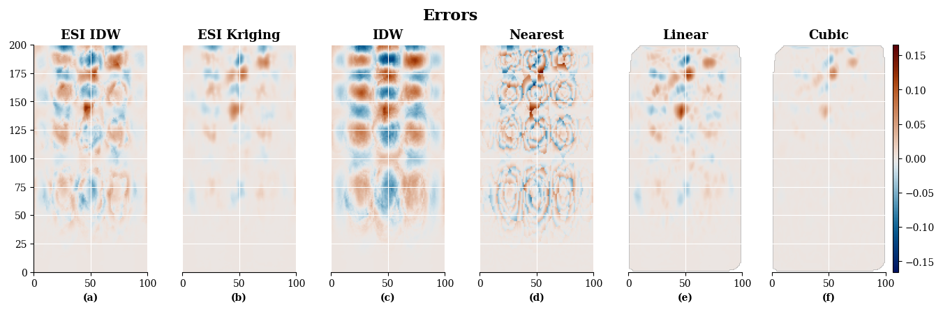
Figure 17 Comparison of ESI and SciPy estimation errors for the same gridded dataset. (a) ESI-IDW interpolation; (b) ESI-Kriging interpolation; (c) IDW interpolation; (d) SciPy nearest-neighbour interpolation; (e) SciPy linear interpolation; (f) SciPy piecewise cubic interpolation.

Figure 17 presents error maps for each method. Notably, the error patterns of methods that failed to fully reproduce the target structure visually – such as ESI-IDW, IDW, and nearest-neighbor interpolation – exhibit the cubic spatial structure itself, indicating their inability to capture it. In contrast, the error maps of ESI-Kriging, linear interpolation, and cubic interpolation show minimal structural patterns, confirming their superior capture of the underlying function. Additionally, all methods exhibit higher errors in areas with more pronounced value gradients.

Finally, Table 2 presents the mean absolute error (MAE), root mean squared error (RMSE), and mean squared error (MSE) for all interpolations. The cubic interpolator achieves the lowest values across all three metrics, which is expected given the cubic nature of the underlying spatial structure. ESI-Kriging achieves the second-best performance, followed by the linear interpolator. Classic IDW demonstrates the highest errors.

Table 2 Performance metrics for ESI and SciPy interpolations for the same gridded dataset.

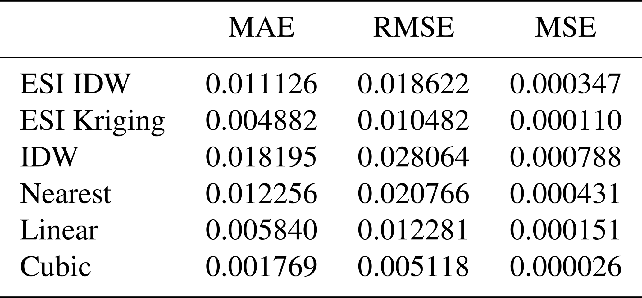
Although ESI-IDW did not achieve exceptional performance in this case study, its superior results relative to traditional IDW highlight the value of the ensemble framework in enhancing the performance of a fundamentally deterministic interpolation method.

4.3 Real-world case study

This section presents the procedure and results from the real-world data case study, demonstrating the use of spatialize on non-gridded data.

4.3.1 Spatialize: ESI-IDW with Mondrian partitioning

We begin by implementing ESI with IDW as local interpolator. As mentioned within Sect. 2.1, both Mondrian Forest and Voronoi Forest can be used as the partitioning method in the case of ESI-IDW⁴. In this first example, we employ Mondrian partitions.

First, we employ the esi_hparams_search() function to obtain optimal parameters for the estimation. The evaluated set is shown in Code snippet 11.

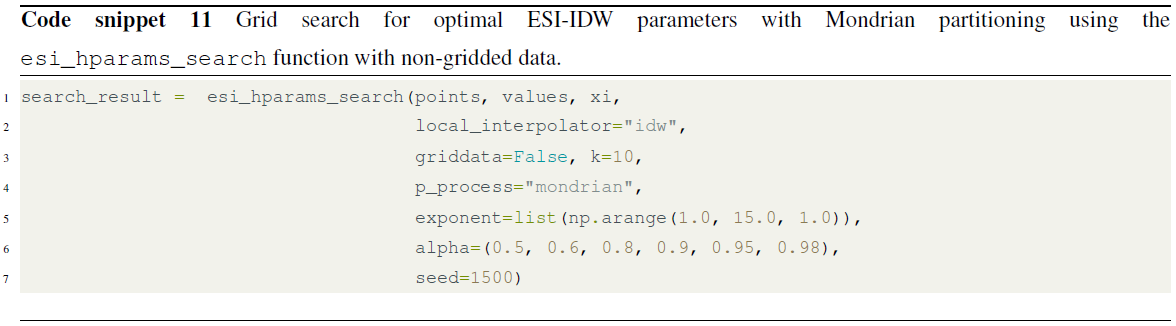
Figure 18 illustrates the cross-validation errors of the 168 search scenarios.

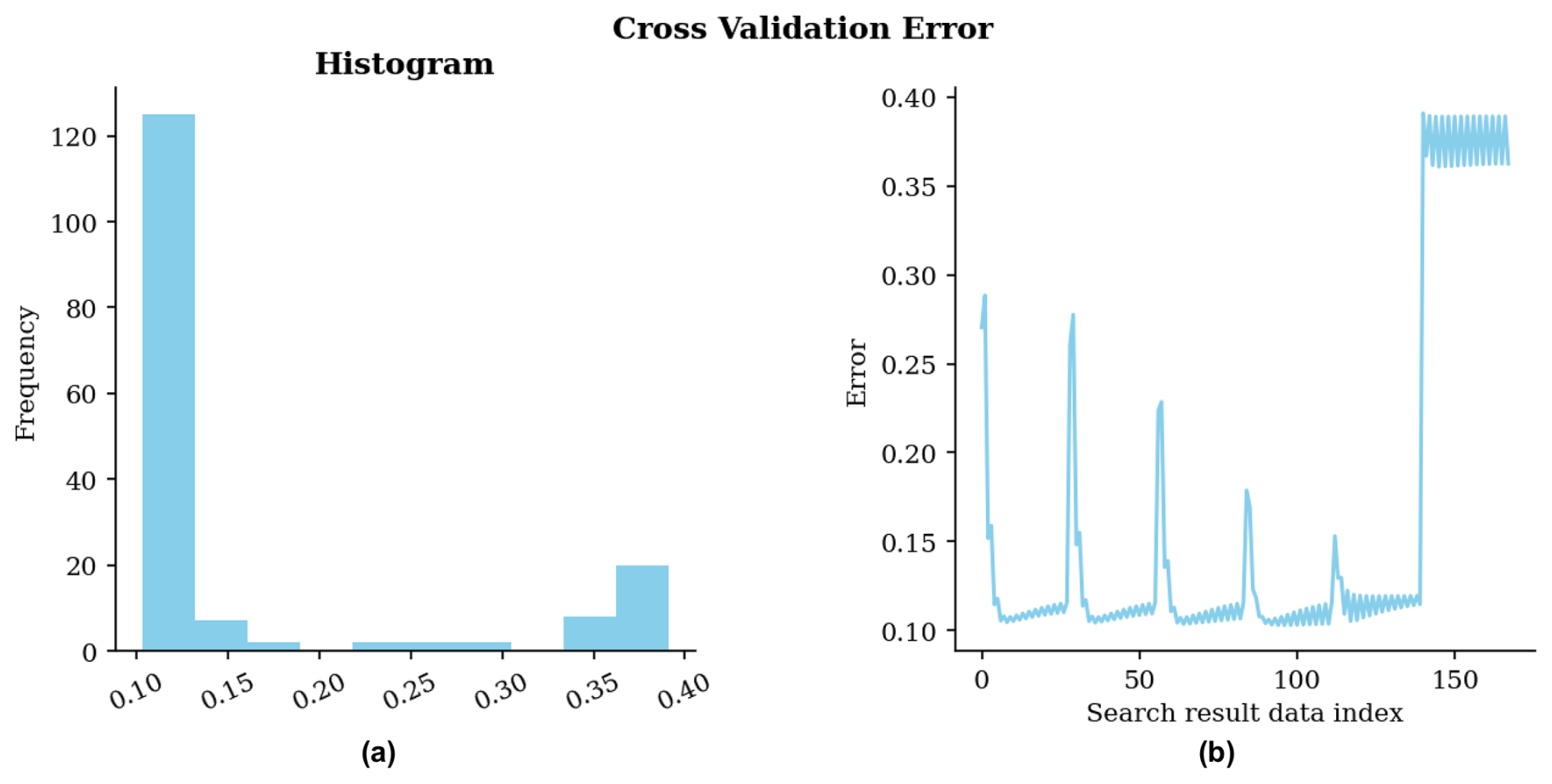
Figure 18 Cross-validation error for the ESI-IDW non-gridded estimation parameter grid search. (a) Histogram of errors; (b) Errors in the sequence of scenarios during the search.

The best-case scenario has the following parameters:

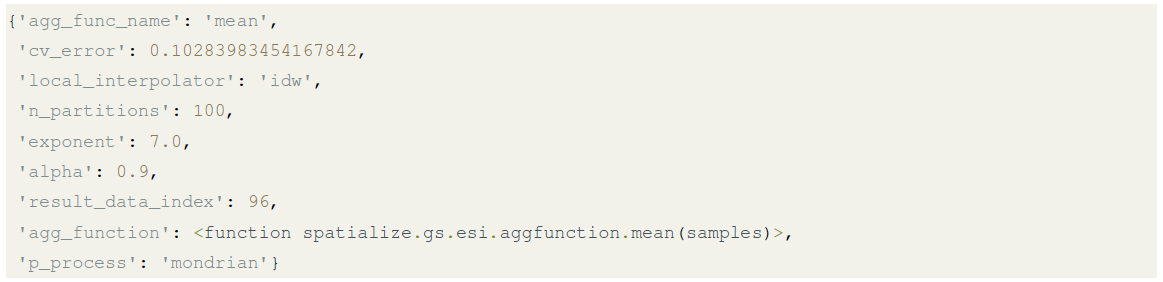
As observed, the optimal exponent for the IDW interpolator is relatively high. Recall that when the exponent equals zero, the local estimate becomes a simple average of all neighbors, producing a smoothing effect similar to Kriging. Conversely, as the exponent approaches infinity, IDW converges to a nearest neighbor estimator, resulting in more abrupt spatial transitions.

With these optimal parameters, we then perform the corresponding estimation using the esi_nongriddata() function, as shown in Code snippet 12.

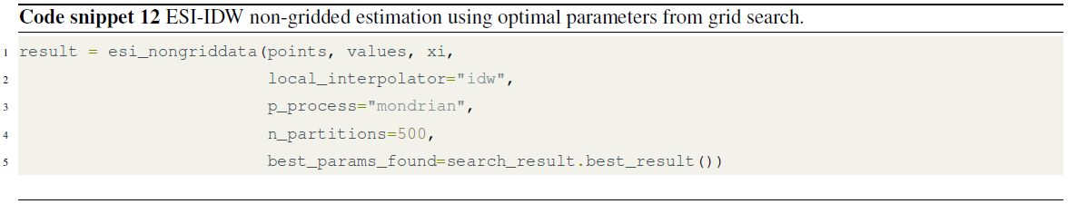
Just like in the gridded-data case, the estimates can be retrieved using the result.estimation() method, while their corresponding precision is obtained through result.precision().

Once we obtain the prediction, we use the lf.OperationalErrorLoss() function to implement the “Operational Error” loss function for ESI precision calculations:

This loss function can then be passed to the precision method: result.precision(op_error).

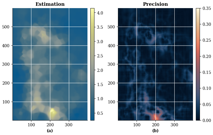
Figure 19 (a) Best parameter non-gridded estimation with ESI-IDW; (b) Precision obtained with operational error loss function.

Figure 19 shows the resulting estimation and the corresponding precision based on the operational error loss function. The figure exhibits a somewhat pixelated texture, which can be attributed to the high optimal exponent value for the local IDW interpolator. The precision map reveals elevated uncertainty near regions corresponding to the maximum estimated values.

4.3.2 Spatialize: ESI-IDW with Voronoi partitioning

We now employ ESI-IDW with Voronoi as the partitioning method, following the same parameter search configuration and estimation procedure described in the Mondrian example.

Figure 20 illustrates the cross-validation errors across the 336 evaluated parameter combinations. Note that the Voronoi partitioning method yields twice the number of search scenarios compared to Mondrian partitioning, as the data_cond parameter offers two options: conditioning the partition on sample locations or using an unconditioned partition.

Figure 20 Cross-validation error for the ESI-IDW non-gridded estimation parameter grid search, using Voronoi partitioning method. (a) Histogram of errors; (b) Errors in the sequence of scenarios during the search.

In this case, the best-case scenario has the following parameters:

As in the previous case using Mondrian partitioning, the optimal exponent for the local interpolator is relatively high, implying that the resulting estimates should exhibit abrupt spatial transitions. However, cross-validation selected a coarser partition for Voronoi (alpha=0.5) than for Mondrian (alpha=0.9). Although the alpha parameter controls partition granularity in both methods, its operational mechanism differs between them, explaining this discrepancy.

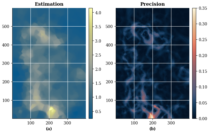
Figure 21 a) Best parameter non-gridded estimation with ESI-IDW; (b) Precision obtained with operational error loss function, this time with Voronoi partition method.

Next, we perform the corresponding ESI estimation using the esi_nongriddata() function with the optimal parameters for Voronoi partitioning. Figure 21 presents the resulting estimates and their associated precision based on the operational error loss function.

As observed with Mondrian partitioning, the estimates exhibit abrupt spatial transitions. However, the precision map exhibits substantially higher values, indicating greater uncertainty in the Voronoi implementation. Whether this elevated uncertainty reflects geometric differences between the partitioning methods or the contrasting optimal alpha remains unclear and requires further investigation.

4.3.3 Spatialize: ESI-Kriging

Analogous to the ESI-IDW case, we present estimates for the ESI-Kriging case, where Kriging serves as the local interpolator for ESI ⁵.

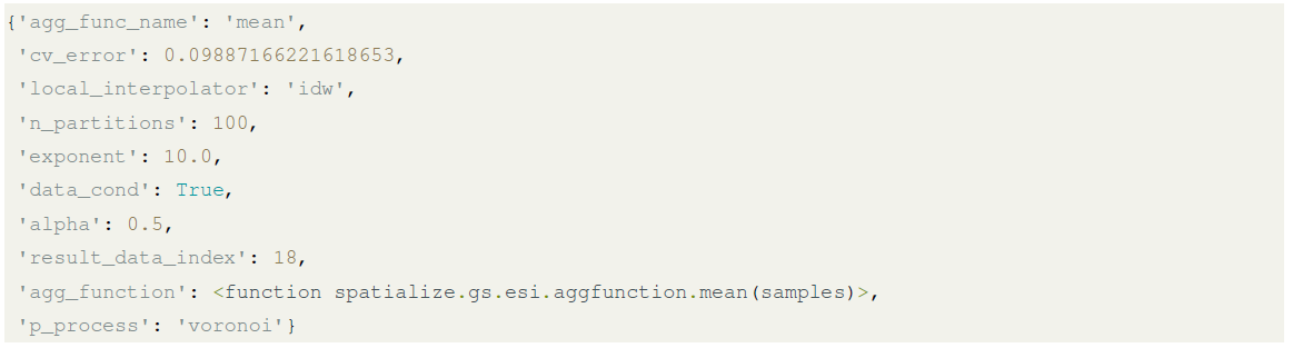
The parameter grid, presented in Code snippet 13, includes four omnidirectional covariance function models, each evaluated across multiple values of alpha, nugget, range, and sill parameters.

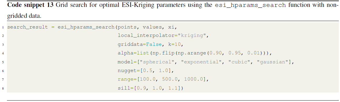
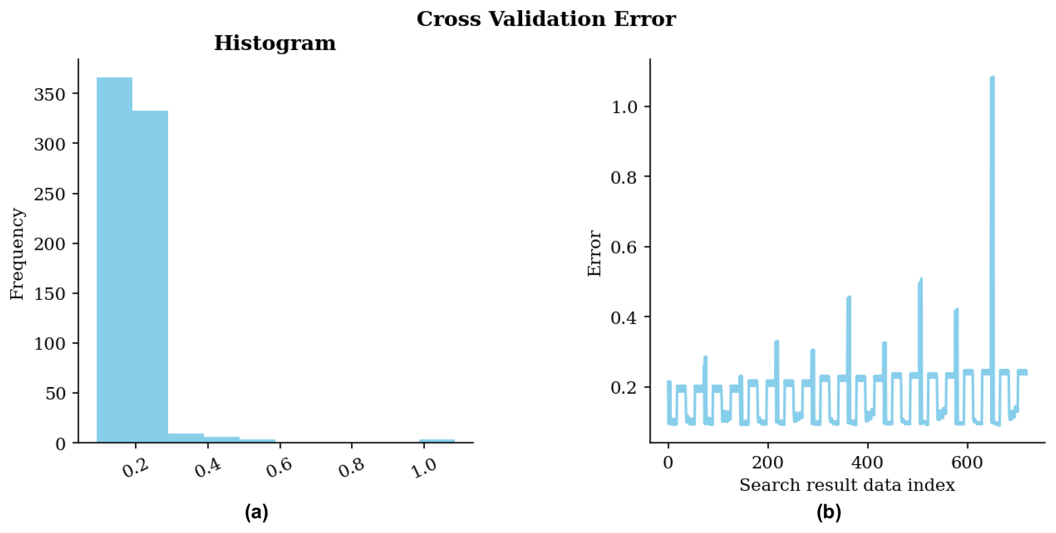
Figure 22 Cross-validation error for the ESI-Kriging non-gridded estimation parameter grid search. (a) Histogram of errors; (b) Errors in the sequence of scenarios during the search.

Figure 22 illustrates the cross-validation error for all evaluated parameter combinations.

In this case, the optimal parameters are:

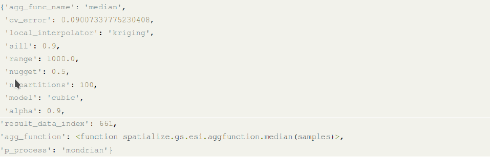
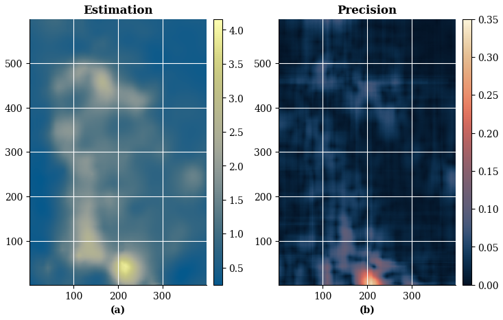
Figure 23 (a) Best parameter non-gridded estimation with ESI-Kriging; (b) Precision obtained with operational error loss function.

Using the optimal parameters, we generate the corresponding estimates via the esi_nongriddata() function. We compute the precision using the operational error loss function, following the same procedure as in the ESI-IDW case. Figure 23 presents the resulting estimation and precision maps. Compared to ESI-IDW, the ESI-Kriging estimates exhibit substantially smoother spatial transitions.

4.3.4 Comparison with Kriging

To compare the ESI estimates against the gold standard method in the mining industry, we now present Ordinary Kriging estimates.

To produce the Ordinary Kriging estimate, an omnidirectional experimental variogram was computed and fitted to a theoretical variogram model comprising two nested spherical structures (Eq. 13).

$$\begin{array}{}\text{(13)}& \begin{array}{rl}\mathit{\gamma }\left(h\right)& ={\text{sill}}_{\mathrm{1}}\left(\mathrm{1.5}{\displaystyle \frac{h}{{\text{range}}_{\mathrm{1}}}}-\mathrm{0.5}{\left({\displaystyle \frac{h}{{\text{range}}_{\mathrm{1}}}}\right)}^{\mathrm{3}}\right)\\ & +{\text{sill}}_{\mathrm{2}}\left(\mathrm{1.5}{\displaystyle \frac{h}{{\text{range}}_{\mathrm{2}}}}-\mathrm{0.5}{\left({\displaystyle \frac{h}{{\text{range}}_{\mathrm{2}}}}\right)}^{\mathrm{3}}\right)\end{array}\end{array}$$

where:

$${\text{sill}}_{\mathrm{1}}=\mathrm{0.17},{\text{ \hspace{0.17em}\hspace{0.17em}\hspace{0.17em}\hspace{0.17em}range}}_{\mathrm{1}}=\mathrm{95},{\text{ \hspace{0.17em}\hspace{0.17em}\hspace{0.17em}\hspace{0.17em}sill}}_{\mathrm{2}}=\mathrm{0.14},{\text{ \hspace{0.17em}\hspace{0.17em}\hspace{0.17em}\hspace{0.17em}range}}_{\mathrm{2}}=\mathrm{220}.$$

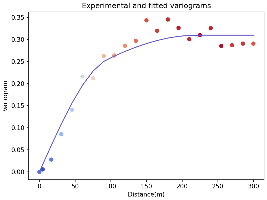
Figure 24 Experimental (dots) and theoretical (blue line) variograms for the Global Ordinary Kriging example.

Both experimental and theoretical variograms are shown in Fig. 24.

Additionally, we have implemented an automated workflow that employs scikit-learn to run a parameter grid search for identifying the optimal variogram model, followed by PyKrige to perform Ordinary Kriging using the identified optimal parameters.

This automated approach differs from the process carried out by the expert in three ways: It uses global Kriging instead of domains depending on local stationarities; it determines variogram parameters in a heuristic way rather than through expert judgment; and it assumes that the variogram is the same in all directions (isotropy), ignoring potential anisotropies in the data. The result obtained for the parameter search is as follows:

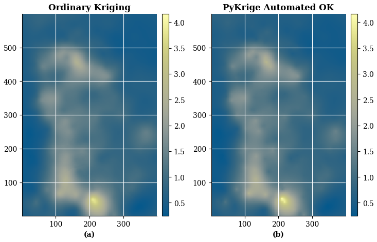
Figure 25 (a) Global Ordinary Kriging estimation based on non-gridded example data points; (b) Automated Kriging estimation with PyKrige.

Figure 25 compares the manual expert implementation of Global Ordinary Kriging (left) – previously presented in (Egaña et al., 2021) – with the automated implementation (right).

As we can see in Fig. 25, the estimation obtained with the automated algorithm is comparable to the ordinary Kriging performed manually on the basis of expert judgment. This is because the example is an ideal case of isotropy and stationarity, i.e. it fulfils the basic assumptions of a linear method such as Kriging.

4.3.5 Performance comparison

This section provides a visual and quantitative comparison of all interpolators employed in the real-world data case study.

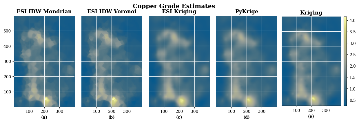
Figure 26 Comparison of ESI and Ordinary Kriging estimates for the same non-gridded dataset. (a) ESI-IDW-Mondrian interpolation; (b) ESI-IDW-Voronoi interpolation; (c) ESI-Kriging interpolation; (d) PyKrige automated Ordinary Kriging interpolation; (e) Ordinary Kriging interpolation.

Figure 26 presents the estimates side-by-side. Both ESI-IDW implementations yield visually similar results characterized by abrupt spatial transitions. In contrast, ESI-Kriging, PyKrige, and Ordinary Kriging produce substantially smoother estimates. Notably, ESI-Kriging exhibits moderately less smoothing than the conventional Kriging approaches, potentially achieving a more favourable balance between spatial continuity and preservation of local variability.

We employed two approaches for quantitative performance evaluation. First, we performed leave-one-out cross-validation with global hyperparameter optimization, as individual optimization for each of the 400 samples would be computationally prohibitive. Second, we conducted 10-fold cross-validation with hyperparameter optimization performed within each fold.

Table 3 presents the mean absolute error (MAE), root mean squared error (RMSE), and mean squared error (MSE) for all automated interpolation methods, obtained using leave-one-out cross-validation. For both ESI and Kriging methods, parameters were determined from the previously conducted grid searches to avoid re-optimization within each fold. Both ESI-IDW implementations achieve comparable performance, although inferior to ESI-Kriging and Ordinary Kriging, with the Mondrian partitioning yielding slightly smaller errors. Ordinary Kriging, implemented with PyKrige, achieves the lowest RMSE and MSE values, while ESI-Kriging achieves the lowest MAE. Since RMSE and MSE penalize larger errors more heavily than MAE, these results suggest that ESI-Kriging produces more accurate estimates on average, but is more susceptible to occasional large prediction errors.

Table 3 Leave-one-out cross-validation performance metrics for ESI and PyKrige interpolations for the same non-gridded dataset.

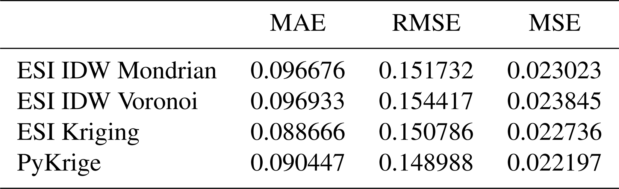
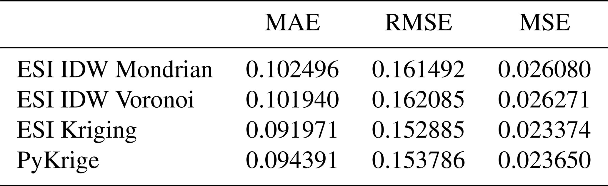
Table 4 presents the mean absolute error (MAE), root mean squared error (RMSE), and mean squared error (MSE) for all automated interpolation methods, obtained using 10-fold cross-validation. ESI-Kriging achieved the best performance across all metrics, followed by PyKrige's Ordinary Kriging. As in the leave-one-out case, ESI-IDW with Mondrian partitioning outperformed the Voronoi method. For all methods and metrics, errors were higher than in the leave-one-out case.

Table 4 K-fold cross-validation performance metrics for ESI and PyKrige interpolations for the same non-gridded dataset (K=10).

Comparing the two validation approaches reveals two key findings.

First, the higher errors across all methods in 10-fold validation – where training datasets are smaller – confirms that interpolation quality decreases with reduced data availability. Second, while ESI-Kriging outperformed PyKrige under 10-fold validation, it showed higher RMSE and MSE under leave-one-out validation. This suggests the ESI ensemble scheme may provide additional benefits when limited data availability makes both parameter optimization and interpolation more challenging. However, these results may be influenced by the specific fold configurations.

Given the ideal conditions in this dataset – isotropy, stationarity, and linear spatial correlation, as confirmed by the expert variogram analysis – one might expect Ordinary Kriging to perform best. However, as observed with IDW in the synthetic data case study, ESI's non-linear ensemble scheme proves beneficial, particularly under limited data availability. Moreover, ESI-Kriging offers competitive performance with automated parameter selection. This provides significant advantages in more complex scenarios involving spatial heterogeneity, where determining appropriate variogram models is challenging or where available models in automatable tools such as PyKrige may be unsuitable.

5 Conclusion and future work

We have introduced spatialize, an open-source Python library that implements ensemble spatial interpolation (ESI), a novel data-driven geostatistical technique grounded in computational statistics and ensemble learning principles. The library addresses a critical gap in geostatistics by providing automated functionality with performance comparable to expert-level methods while quantifying prediction uncertainty.

The primary strength of spatialize lies in its minimal requirement for user intervention, enabling researchers without specialized geostatistical expertise to obtain optimal spatial predictions. In cases where user input is necessary – such as hyperparameter selection – the library provides tools that facilitate the process.

Our vision is for spatialize to become one of the leading open-source geostatistical libraries available in Python. To this end, future work includes the following enhancements:

• Implement additional partition generation processes, such as Mondrian processes with random rotations, to increase the expressiveness and diversity of space partitions.

• Integrate adaptive local interpolators to improve performance in heterogeneous spatial domains.

• Incorporate interpolators compatible with spatial statistical tools, including conditional autoregressive (CAR)-type models.

• Extend functionality to accommodate the estimation of categorical variables.

• Implement GPU support to enhance computational performance and enable seamless integration with platforms such as Google Colab.

• Provide classical geostatistical tools for expert users, including more general Kriging implementations that support nested structures and other advanced configurations.