Biogeodynamics-Ice sheet-Geneva-MITgcm (BIG-MITgcm, v1.0): a simulation tool for exploring climate states with a representation of global ice sheets

Modelling the climate system on multi-millennial timescales is challenging when slow-response components, such as the deep ocean, vegetation, and ice sheets, must evolve alongside fast-response components such as atmospheric weather systems. This is crucial for investigating, for example, the dynamical structure of Earth's climate, including steady states, mapping the attractor of those states in a multi-dimensional phase space, and their response to external forcing and internal variability. Earth system models, such as those used in the Coupled Model Intercomparison Project (CMIP), are often too computationally expensive for simulations spanning many thousands of years. Moreover, simplified parameterizations and coarse resolutions typically employed in Earth Models of Intermediate Complexity (EMICs) can adversely affect the nonlinear interactions among the various climate components. Here, we describe a new tool, Biogeodynamics-Ice sheet-Geneva-MITgcm – or BIG-MITgcm for short – which attempts to fill in the hierarchy between these two classes of model. The core of BIG-MITgcm is a coupled MITgcm setup that includes atmospheric, ocean, thermodynamic sea ice, and land modules. To this, we asynchronously couple a vegetation model (BIOME4), a hydrological model (pysheds), and a new global-scale ice sheet model (MITgcmIS). The latter is implemented on the same cubed-sphere grid as MITgcm, using the shallow-ice approximation, and driven by a modified Positive Degree Day method to evaluate the ice-sheet surface mass balance. Here, we present a detailed description of the new ice sheet model and the coupling procedure employed. We evaluate BIG-MITgcm using a pre-industrial simulation initialized from observations of bedrock topography, together with a forced simulation over the 1979–2009 period. The model spontaneously grows plausible ice sheets. These two experiments allow us to assess the model's performance against CMIP-class models, as well as a combination of reanalyses and observations. To evaluate the ability of our model to represent completely different climate conditions and continental configurations, we also discuss a Permian-Triassic solution with a small ice sheet in the Northern Hemisphere. In summary, BIG-MITgcm successfully captures many large-scale properties of the current climate, suggesting that it will be a very useful tool for exploring current, past, and future climates. We conclude by discussing potential applications and future developments.

1 Introduction

As atmospheric CO₂ concentrations rise from the pre-industrial era, there is a potential risk of crossing critical thresholds in which key parts of the climate system may suddenly change, potentially irreversibly (Wunderling et al., 2024). It is important, therefore, to understand the dynamical structure of Earth's climate in which possibly different climate states (attractors) co-exist with the same external forcing (e.g. CO₂), the limits of their existence (basins of attraction), and boundaries beyond which forcing shifts climate into a different steady state. Reaching a true steady state is an important property for characterizing climatic attractors (Hawkins et al., 2011; Drótos et al., 2017; Lucarini and Bódai, 2017; Brunetti et al., 2019; Brunetti and Ragon, 2023; Moinat et al., 2024). However, to reach equilibrium among all the components of climate, and particularly those with very slow response times, such as the deep ocean, terrestrial vegetation, or ice sheets, experiments must be carried out on millennia time scales. This requires dedicated modeling techniques.

Here, we are interested in a modeling framework that allows us to explore global climate dynamics in which, for example, ice sheets are not necessarily confined to high latitudes but can spread equatorwards as in glacial periods, waterbelt or snowball states. The model must be able to span from daily to millennial timescales on global spatial scales, and include atmosphere, surface, and deep ocean, sea ice, land vegetation, and ice sheet dynamics. Although these components are sometimes included in CMIP-like models (Eyring et al., 2016), such models are very demanding of computational resources and solutions cannot reach stationarity in the sluggish deep-ocean and/or ice sheets (Balaji et al., 2017). In contrast, Earth Models of Intermediate Complexity (EMICs) can economically reach a stationary state (Claussen et al., 2002; Willeit et al., 2022), but their typically coarse spatial resolution (∼500 km) and highly simplified parameterizations may have non negligible impacts on the nonlinear interaction among climatic components.

Currently, there are few CMIP6 models with interactive ice sheets (e.g. Ackermann et al., 2020; Muntjewerf et al., 2020; Madsen et al., 2022; Smith et al., 2021) and/or dynamical vegetation (Drüke et al., 2021). However, extreme computational cost makes such models inappropriate for studying climate evolution on millennial timescales. A technique for speeding up models in which components with disparate timescales are brought together is asynchronous coupling (Claussen, 1994; Herrington and Poulsen, 2011; Pohl et al., 2016; Sommers et al., 2021). In such an approach, for example, the climate is first computed with fixed ice sheets and vegetation, and the latter are then updated to match the equilibrium conditions of the former (Foley et al., 1998). The procedure is repeated until convergence. In this way, fast and slow components evolve consistently until a stationary state is reached.

Here, we describe a simulation tool, which we call Biogeodynamics-Ice sheet-Geneva-MITgcm (or BIG-MITgcm for short), that couples ice sheets, surface processes, vegetation, and climate dynamics on multi-millennial timescales, with a state-of-the-art ocean and simplified atmospheric parameterizations. It has a high vertical resolution in the ocean and a finer spatial resolution than traditional EMICs (Holden et al., 2016; Willeit et al., 2022). The model employs asynchronous coupling with a vegetation model and a newly developed global-scale ice sheet model. In so doing, it consistently draws together the evolution of key Earth processes on multi-millennial time scales: vegetation, atmosphere, ocean, cryosphere, hydrosphere, and their interactions, under different boundary conditions given by continental and ocean basin configurations. We have designed the system so that is can also be used to investigate deep-time climates, which are characterized by large uncertainties in initial conditions, especially for ice sheets and vegetation. We provide a short description of the dynamical core (based on MITgcm), the vegetation model (BIOME4) and the hydrology model (pysheds): these have already been described in detail elsewhere. Our focus here is on the ice sheet model (MITgcmIS). To assess the ability of BIG-MITgcm to represent the present climate, we compare its climate state to those of some CMIP6 class models and reanalysis products. In addition, to showcase its ability to simulate ice sheets that might develop in a world of very different continental configuration and climate conditions, the climate state appropriate to a Permian-Triassic paleogeography based on Ragon et al. (2024) is described.

2 Details of the BIG-MITgcm simulation tool

Here, we describe each component of our coupled model, including the boundary conditions employed and the coupling strategy.

2.1 GCM – coupled MITgcm setup

The dynamical core is the MIT general circulation model (MITgcm) (Marshall et al., 1997a, b; Adcroft et al., 2004), which solves the Navier–Stokes equations for the atmosphere and the ocean on the same cubed-sphere (CS) grid (Marshall et al., 2004). In particular, we deploy MITgcm (version c68s) in a coupled setup including atmosphere, ocean, thermodynamic sea ice, and land (denoted as Coupled MITgcm Setup). We use the so-called CS32 configuration, where each face of the cube has 32×32 grid cells, corresponding to an average horizontal resolution of 2.8°. This or similar configurations have already been used for studying idealized configurations such as the coupled aquaplanet (Marshall et al., 2007; Rose, 2015; Ferreira et al., 2011, 2018; Brunetti et al., 2019; Ragon et al., 2022; Zhu and Rose, 2023; Brunetti and Ragon, 2023; Moinat et al., 2024), deep-time climates (Brunetti et al., 2015; Ragon et al., 2024, 2025), and the present-day climate (Brunetti and Vérard, 2018).

Physical parameterizations for the atmosphere are based on the 5-layer SPEEDY model (Simplified Parameterizations, privitivE-Equation DYnamics) (Molteni, 2003). SPEEDY is a model of intermediate complexity for the atmosphere, and includes simplified representations of convection, large-scale condensation, vertical diffusion, surface fluxes of momentum and energy. The radiative scheme uses two spectral bands for the shortwave radiation and four for the longwave radiation. Cloud cover and thickness are defined diagnostically from the values of relative and absolute humidity. The cloud albedo depends on latitude, as done in Ragon et al. (2022), to reduce net solar radiation at high latitudes and therefore to have better agreement with observational data (Kucharski et al., 2013). Five pressure levels are represented, from 1000 hPa to 0 Pa, where the bottom level represents the planetary boundary layer, the upper one the stratosphere and the remaining three the free troposphere. SPEEDY has been evaluated against the NCEP-NCAR and ERA5 reanalysis (Molteni, 2003) and, despite its simplified parameterizations, has been assessed to provide a realistic description of the atmosphere, with the advantage of requiring fewer computer resources than state-of-the-art Atmospheric GCMs. A simple 2-layer land model (Hansen et al., 1983) is coupled to SPEEDY.

The physics packages used in the ocean component are the K-profile parameterization scheme (Large and Yeager, 2004) to account for vertical mixing in the water column and the Gent and McWilliams scheme  (Gent and McWilliams, 1990) to capture residual-mean circulation and mixing by mesoscale eddies. The Winton model (Winton, 2000) is used to represent sea ice thermodynamics (THSICE), while sea ice dynamics is neglected. In our setup, there are 25 vertical nonuniform levels in the ocean, with thickness ranging between 20 m near the surface and 1300 m at the bottom.

The Coupled MITgcm Setup requires the following boundary conditions: bare-surface albedos, vegetation fraction, bathymetry, topography, runoff routing map, salinity, and ocean temperature for all ocean levels (the latter two files are used to initialize the coupled model and then updated by the dynamical core as the integration proceeds). Orbital parameters can be set by specifying obliquity, precession, and eccentricity. In addition, the duration of the day and the solar incoming radiative influx can be modified. The whole system runs at a speed of about 200 years per day using 25 cores, which is equivalent to 300 CPU hours for 100 simulated years.

2.2 Boundary conditions – land-ocean configuration

Our model can be applied to the present-day and deep-time climates using different paleogeographies. Although the present day observed continental configuration is well known, we employ reconstructions of paleogeography for deep-time climates. Several options are available (Vérard, 2019; Scotese, 2021; Merdith et al., 2021). Although in previous studies MITgcm made use of the PANALESIS reconstructions (Brunetti et al., 2015; Brunetti and Vérard, 2018; Ragon et al., 2024, 2025), the model can be initialized using any boundary conditions (i.e. alternative paleogeographical reconstructions, idealized land-ocean configurations, or aquaplanet) and ocean depths, which is useful for exoplanet or conceptual studies.

In both present-day and deep-time applications, the procedure for adapting the high resolution geographical maps to the MITgcm grid is the same. Using the present-day ETOPO global relief model (ETOPO, 2022) or a paleogeographic reconstruction, the input geography is given in a latitude/longitude coordinate system with arc-sec horizontal resolution. Since simulations are performed with the cubed-sphere CS32 grid, interpolation and smoothing are used to upscale the resolution to 2.8° (Ragon, 2024). Then, isolated oceanic points or lakes are removed, irrespective of their size, to avoid numerical instability when there are enclosed areas of water. Moreover, very shallow waters are also prone to instability, especially when sea ice develops; all oceanic points shallower than −20 m are set to this depth.

2.3 Vegetation – BIOME4

BIOME4 is a vegetation model that predicts the global steady state of the vegetation distribution corresponding to long-term averages of monthly mean 2-m air temperature (denoted as surface air temperature in the following or SAT), sunshine and precipitation (Kaplan, 2001). Additional inputs are soil depth and texture, which are used to determine water holding capacity and percolation rates (Kaplan et al., 2003). Moreover, the atmospheric CO₂ content needs to be specified. All these quantities are obtained from steady-state simulations performed using MITgcm in the coupled configuration described in Sect. 2.1. Bare-surface albedos and the vegetation map obtained as outputs of BIOME4 are then reused in the next iteration of the coupling system. Water holding capacity and percolation rates are kept constant in our simulations and set to the present-day average value.

BIOME4 follows the principle that ecosystems can be divided into a set of biomes characterised by the performance of plant functional types (PFTs), i.e. key parameters used to classify plant species having a similar response to the environment (Haxeltine and Prentice, 1996; Kaplan, 2001). The model selects among a set of 12 PFTs the subset that can be present in a grid cell on the basis of physiological and climatic constraints, like minimal temperature and water supply. Using a coupled carbon and water flux model, BIOME4 calculates the net primary productivity (NPP) of each PFT and the corresponding seasonal maximum leaf area index (LAI) that maximises NPP. At this point, competition among PFTs is simulated by selecting the PFT with the optimal NPP as the dominant plant type. Opposing effects due to light competition and wildfires are included through semi-empirical rules. The final output is the vegetation distribution in terms of the dominant and secondary PFTs, total LAI and NPP, which can be classified into biome types, for a total of 27 biomes (28 including land ice). Land-ice points are determined by the ice sheet extent computed by MITgcmIS (see next section). Therefore, the grid points that are identified as land ice overwrite the biome number given by BIOME4.

Main differences between BIOME4 and earlier versions (developed by Prentice et al., 1996; Haxeltine and Prentice, 1996) are the inclusion of new PFTs to represent vegetation types in the polar regions, and the calculation of photosynthetic pathways (for C₃ and C₄ plants) that depend on the PFT. BIOME4 and its earlier versions have been used to investigate climate-biosphere interactions in the past (de Noblet-Ducoudré et al., 2000; Haywood et al., 2002; Kaplan et al., 2003; Salzmann et al., 2008; Sellwood and Valdes, 2008), and coupled to MITgcm in Ragon et al. (2024, 2025) for the Permian-Triassic Boundary. BIOME4 has also been used to assess the impact of current climate changes on the distribution of vegetation types (Allen et al., 2024).

2.4 Ice sheet – MITgcmIS

We have developed a Python code, called MITgcmIS, that describes the evolution of ice sheets at the global scale on the same cubed-sphere grid used by MITgcm. A global-scale ice sheet model is required when the climate state allows for the presence of ice sheets at low latitudes, for example during glaciation periods, waterbelt states or snowball states (Kirschvink, 1992; Hoffman and Schrag, 2002). Since we are interested in simulating the main processes occurring at spatial resolutions of around 2° or coarser, we neglect basal melting and other fine-scale processes, as calving and ice streams, since they cannot be resolved at such coarse resolutions. Note that there is already an MITgcm module, called STREAMICE, which implements in Fortran these small-scale processes at the km-scale (Goldberg and Heimbach, 2013), however this package is not used in our coupled setup.

In MITgcmIS, we use the shallow-ice approximation (Cuffey and Paterson, 2010) to model the ice-sheet movement and the Positive Degree Day (PDD) method (Braithwaite, 1977) to compute the surface mass balance. In particular, we choose the PDD approach as described in Tsai and Ruan (2018) instead of the Surface Energy Balance (SEB) method, since the latter requires quantities at the km-scale to estimate the energy budget, such as layer structure, surface roughness, and stability of the surface terrain to obtain latent and sensible heat fluxes (Hock and Holmgren, 2005). Thus, the SEB method is generally used in regional climate models, which are able to reach the required accuracy in the representation of the climatic fields (especially clouds), in general provided by reanalyses (Wake and Marshall, 2015).

Although the PDD approach succeeds in representing the surface mass balance in coarse simulations, it can underestimate the melting in past periods of high insolation (Plach et al., 2018). Moreover, since this method does not account for energy exchanges between the ice sheet and the other components of the climate system, it cannot ensure a closed energy budget. Despite its limitations, we believe that the PDD method is the best choice when the representation of the atmosphere and snow processes are at the global scale on a coarse grid and simplified as in the SPEEDY and land modules (Sect. 2.1).

2.4.1 Basic description

We start from the equation that describes the depth-integrated mass conservation for incompressible ice (Schoof and Hewitt, 2013):

$$\begin{array}{}\text{(1)}& {\displaystyle }{\displaystyle \frac{\mathrm{d}H}{\mathrm{d}t}}=-\mathbf{\nabla }\cdot \mathit{q}+\dot{A}-\dot{B}\end{array}$$

where $H=z_{\mathrm{S}}-z_{\mathrm{B}}$ is the height of the ice sheet between the bed z_B and the surface z_S vertical coordinates, $\mathit{q}={\int }_{z_{\mathrm{B}}}^{z_{\mathrm{S}}}\mathit{U}\mathrm{d}z$ is the horizontal flux obtained by vertical integration over the ice thickness of the horizontal part U of the velocity vector, $\dot{A}$ is the surface mass balance rate and $\dot{B}$ is the basal melting rate. In our case, we neglect the basal melting rate, hence $\dot{B}=\mathrm{0}$. Equation (1) is simply an expression of mass continuity; but the specific form of q derives from the full Stokes equations in the so-called shallow-ice approximation, based on the low aspect ratio ($\sim {\mathrm{10}}^{-\mathrm{2}}$–10⁻³) between vertical and horizontal length in ice sheets. This relationship describes how ice flux responds to ice-sheet geometry, as described below.

Ice deformation can be simplified by neglecting basal sliding, by considering that the only important type of deformation is vertical shearing, and by assuming a power-law shear thinning viscous rheology, with strain rates $\dot{\mathit{ϵ}}$ proportional to the driving stress τ_d, as $\dot{\mathit{ϵ}}=a|{\mathit{\tau }}_{\mathrm{d}}{|}^{n-\mathrm{1}}{\mathit{\tau }}_{\mathrm{d}}$, where a is the Glen's law coefficient, which is assumed constant, and n is typically set to 3. This leads to the following relation (Cuffey and Paterson, 2010):

$$\begin{array}{}\text{(2)}& {\displaystyle }{\displaystyle }\mathit{q}={\displaystyle \frac{\mathrm{2}a}{n+\mathrm{2}}}|{\mathit{\tau }}_{\mathrm{d}}{|}^{n-\mathrm{1}}{\mathit{\tau }}_{\mathrm{d}}{H}^{\mathrm{2}}=-D\mathbf{\nabla }{z}_{\mathrm{S}}\end{array}$$

where ${\mathit{\tau }}_{\mathrm{d}}=-{\mathit{\rho }}_{\mathrm{i}}gH\mathbf{\nabla }{z}_{\mathrm{S}}$, ∇z_S is the surface slope, g the gravitational acceleration, ρ_i=920 kg m⁻³ the ice density, and

$$\begin{array}{}\text{(3)}& {\displaystyle }{\displaystyle }D={\displaystyle \frac{\mathrm{2}a}{n+\mathrm{2}}}\left({\mathit{\rho }}_{\mathrm{i}}g{)}^n\right|\mathbf{\nabla }{z}_{\mathrm{S}}{|}^{n-\mathrm{1}}{H}^{n+\mathrm{2}}.\end{array}$$

By combining the two relations, one obtains

$$\begin{array}{}\text{(4)}& {\displaystyle }{\displaystyle \frac{\mathrm{d}H}{\mathrm{d}t}}=\mathbf{\nabla }\cdot \left(D\mathbf{\nabla }H\right)+\mathbf{\nabla }\cdot \left(D\mathbf{\nabla }{z}_{\mathrm{B}}\right)+\dot{A}.\end{array}$$

Equation (4) is numerically integrated in Python on the cubed-sphere grid, once the surface mass balance rate $\dot{A}$ is determined, as detailed in the next section.

As noted above, we do not consider spatially varying Glen's law parameter a or basal sliding. Both processes are sometimes included in modelling of paleo ice sheets, by employing thermomechanical components to model ice temperature (which influences Glen's law, Cuffey and Paterson, 2010), and to determine where basal sliding occurs due to thawed-bed conditions (e.g. Moreno-Parada et al., 2023). However, the coarse resolution of our numerical grid does not allow one to represent the fast streaming that results from basal melting. Since our purpose is to investigate climatic steady states in which ice sheets are in balance with the ocean, atmosphere, and biosphere, through their impacts of global albedo, large-scale orography and freshwater fluxes, we choose not to represent these km-scale processes. Moreover, the inclusion of such processes would introduce additional uncertain quantities and formulations – such as the temperature dependence of a, the pattern and magnitude of geothermal heat flux, and the response of basal stress to basal water formation and drainage. Instead, using a single parameter, a, to describe ice-sheet dynamics allows it to be constrained straightforwardly using ice volume, as shown in Sect. 3.2.

2.4.2 Surface mass balance

To compute the surface mass balance we use a method based on the Positive Degree Day (PDD), which has in addition a percolation layer for correctly assessing the melting (Tsai and Ruan, 2018).

The idea of this PDD method is to account for the presence of a percolation layer of thickness H_p that creates a delay in melting at the ice surface, as the ice is not expected to melt as soon as the SAT reaches 0 °C (Tsai and Ruan, 2018). The heat is assumed to be diffused downwards in the percolation layer, which reaches a uniform temperature T_p on a relatively fast timescale. In our setup, we assume that the percolation depth H_p is constant even if in reality it can slightly change, depending on the type of ice. Below the percolation depth, the temperature quickly relaxes to an equilibrium value that does not depend on diffusion (Tsai and Ruan, 2018).

We assume that, between the ice surface (z=0) and the height where the temperature measurement is performed (z=h), there is a constant temperature gradient. Thus, the heat flux can be written as:

$$\begin{array}{}\text{(5)}& {\displaystyle }{\displaystyle }q\left(t\right)=-k{\displaystyle \frac{\partial T}{\partial z}}=-k{\displaystyle \frac{T_a\left(t\right)-T_{\mathrm{p}}\left(t\right)}{h}}\end{array}$$

where k is the effective thermal conductivity of air, T_a is the temperature at z=h, and T_p is the percolation layer temperature. From this assumption, and using conservation of energy between the percolation layer and the air, one can compute the ordinary differential equations for the percolation layer temperature T_p and for the ablation rate a_r (Tsai and Ruan, 2018):

$$\begin{array}{}\text{(6)}& {\displaystyle }& {\displaystyle \frac{\mathrm{d}{T}_{\mathrm{p}}}{\mathrm{d}t}}={\displaystyle \frac{k}{h{\mathit{\rho }}_{\mathrm{i}}{c}_P{H}_{\mathrm{p}}}}(T_a-T_{\mathrm{p}})\text{ if }{T}_{\mathrm{p}}<\mathrm{0}\text{ or }{T}_a<\mathrm{0}\text{(7)}& {\displaystyle }& {\displaystyle }{a}_{\mathrm{r}}\left(t\right)=-{\displaystyle \frac{\mathrm{d}{z}_{\mathrm{S}}}{\mathrm{d}t}}={\displaystyle \frac{k}{h{\mathit{\rho }}_{\mathrm{i}}L}}(T_a-T_{\mathrm{p}})\text{ if }{T}_{\mathrm{p}}=\mathrm{0}\text{ or }{T}_a>\mathrm{0}\end{array}$$

where z_S is the ice surface elevation. Constants k, h, ρ_i, c_P, H_p, and L are all assumed to be known. We have used ρ_i=920 kg m⁻³, c_P=2100 $\mathrm{J}{\mathrm{kg}}^{-\mathrm{1}}\mathrm{°}{\mathrm{C}}^{-\mathrm{1}}$, and L=334 kJ kg⁻¹ as in Tsai and Ruan (2018), and we set $k/h=\mathrm{40}$ $\mathrm{W}{\mathrm{m}}^{-\mathrm{2}}\mathrm{°}{\mathrm{C}}^{-\mathrm{1}}$, H_p=10 m, and h=2 m in our setup. The required input is the air temperature T_a at h=2 m, which is an MITgcm output. Tsai and Ruan (2018) showed good agreement with observations, along with a significant improvement in capturing early-season melting compared to the classical PDD method. During each model iteration, we compute the surface mass balance by including the lapse rate effect that accounts for changes in surface elevation (see Sect. 2.4.3).

To determine the remaining contribution to the surface mass balance, we evaluate the accumulation of snow. This quantity is obtained by using outputs from the Coupled MITgcm Setup. To be consistent with the energy budget in the MITgcm, the accumulation is estimated from the snow precipitation per grid cell. Since the MITgcm land module does not include accurate snow physics and, in particular, a process that densifies snow over time to obtain glacial ice, this densification is assumed to happen instantaneously. Therefore, as snow precipitation is expressed in units of [$\mathrm{kg}{\mathrm{m}}^{-\mathrm{2}}{\mathrm{s}}^{-\mathrm{1}}$], we divide this quantity directly by the glacial ice density, ρ_i=920 kg m⁻³ to obtain the accumulation rate in [m s⁻¹ ice equivalent]. Rain over the ice sheet cannot be freezed and is handled by the runoff routing scheme in Sect. 2.5.

In summary, two MITgcm outputs are needed: the 2-m air temperature (for the ablation) and the snow precipitation (for the accumulation). These two quantities are extracted from a simulation that has reached a steady state. We take daily outputs over an interval of 30 years, and then we take the average of these quantities for each day and each grid cell. Finally, the surface mass balance rate $\dot{A}$ is obtained by subtracting the ablation from the accumulation rates, and inserted at the right-hand side of Eq. (4), which is then solved in terms of the ice thickness H.

2.4.3 Isostatic adjustment, lapse-rate, freshwater and sea-level corrections

Taking into account the isostatic adjustment due to the ice sheet mass can be computed in several ways. Here, we adopt the Local Lithosphere Relaxing Asthenosphere (LLRA) method, where a time delay is included (Greve and Blatter, 2009). The idea behind this method is that there is a vertical displacement w_ss (measured in meters) of the lithosphere that is due to the ice load. A steady state is reached when the buoyancy force equilibrates the ice load (Greve and Blatter, 2009):

$$\begin{array}{}\text{(8)}& {\displaystyle }{\displaystyle }{\mathit{\rho }}_{\mathrm{a}}g{w}_{ss}={\mathit{\rho }}_{\mathrm{i}}g\mathrm{\Delta }{H}_{\text{ice}}\end{array}$$

where ρ_i=920 kg m⁻³ is the ice density, ρ_a=3300 kg m⁻³ is the density of the asthenosphere and ΔH_ice is the ice thickness calculated by the ice sheet model. Thus

$$\begin{array}{}\text{(9)}& {\displaystyle }{\displaystyle }{w}_{ss}={\displaystyle \frac{{\mathit{\rho }}_{\mathrm{i}}}{{\mathit{\rho }}_{\mathrm{a}}}}\mathrm{\Delta }{H}_{\text{ice}}.\end{array}$$

However, the response of the asthenosphere is not immediate due to its viscous properties, and has a time delay that can be parameterised as:

$$\begin{array}{}\text{(10)}& {\displaystyle }{\displaystyle \frac{\mathrm{d}w}{\mathrm{d}t}}=-{\displaystyle \frac{\mathrm{1}}{{\mathit{\tau }}_a}}(w-w_{ss})\end{array}$$

where τ_a is typically set to 3000 years (Greve and Blatter, 2009). At each time step Δt=1 yr of MITgcmIS, the ice sheet elevation is computed as:

$$\begin{array}{}\text{(11)}& {\displaystyle }{\displaystyle }{H}_{\text{total}}=H_{\text{topo}}+\mathrm{\Delta }{H}_{\text{ice}}-{\displaystyle \frac{\mathrm{d}w}{\mathrm{d}t}}\mathrm{\Delta }t\end{array}$$

where H_topo is given by the bedrock topography file, which for deep-time climates corresponds to paleogeography reconstructions (Vérard, 2019; Scotese, 2021; Merdith et al., 2021).

As the surface elevation is varied when an ice sheet develops by Δz, not only the topography changes but also the 2-m air temperature. Thus, the effect due to the lapse rate $dT/dz$ needs to be included, as follows:

$$\begin{array}{}\text{(12)}& {\displaystyle }{\displaystyle }{T}_n=T_{n-\mathrm{1}}-{\displaystyle \frac{\mathrm{d}{T}_{n-\mathrm{1}}}{\mathrm{d}z}}\mathrm{\Delta }z\end{array}$$

where T_n is used to run the ice sheet model, and the lapse rate is computed at each ice-sheet grid point using the MITgcm output T_n−1 of the previous iteration. A temperature value is extracted from each pressure level in the atmosphere, and then, using the relation between pressure and altitude, the slope of the linear regression (zonally averaged) is used to estimate the lapse rate.

Finally, since some ice-sheet volume V_ice may have formed or disappeared, the amount of water V_water that has been exchanged with the ocean is estimated by $V_{\text{water}}=V_{\text{ice}}{\mathit{\rho }}_{\text{ice}}/{\mathit{\rho }}_{\text{water}}$. To guarantee the conservation of salt, a volume compensation (Mehling et al., 2026) is performed, $S_n=S_{n-\mathrm{1}}{V}_{n-\mathrm{1}}/V_n$, where S_n and V_n are the global salinity and ocean volume at iteration n, respectively. The variation of water volume in the ocean is converted in sea level change, with updated coastlines defining new topography (including ice sheet height), mask and bathymetry files.

2.5 Runoff – pysheds

In our study, we need to consider different continental configurations corresponding to the Earth's evolution, under a range of ice sheet loading. Hence, for each new configuration, we need to recalculate the runoff map. The Coupled MITgcm Setup needs as an input a file with three arrays, specifying for each land point L_i the corresponding precipitation storage area A_i and the ocean point O_i where it is drained (outlet point).

For present-day as well as for past (palæo-) topographies, we discriminate between land and ocean points by defining a contour line at 0 m in elevation. If any area with negative values are fully enclosed within area with positive values, they are considered as “lakes” (unless elevation reaches values below −2000 m). In such cases, we re-assign the elevation (without affecting the ocean volume) in order to remove the depression and reroute the flow direction. For this purpose, as well as for cleaning local pits, depressions and flat terrains are corrected using the fill_pits, fill_depressions, and resolve_flats functions from pysheds (Bartos, 2020). This ensures a continuous Digital Elevation Model (DEM) with no single pixel or stagnant areas where water would not flow. Finally, we clip the DEM to all elevations above 0 m and retrieve the closest outlet point.

Every point in the MITgcm grid is hence defined as “continental” or “oceanic” depending on whether or not it is located inside the land (positive elevation) or not. Using the corrected topography, we generate a flow direction by applying an eight-direction (D8) flow routing algorithm from pysheds. This method assumes that water from each cell in the DEM will flow to one of its eight neighboring cells, the one that results in the steepest descent. The D8 algorithm is computationally efficient and widely used for hydrological modelling.

The slope from a cell c to each of its eight neighbors i is calculated as:

$$\begin{array}{}\text{(13)}& {\displaystyle }{\displaystyle }{s}_i={\displaystyle \frac{Z_{\mathrm{c}}-Z_i}{d_i}}\end{array}$$

where Z_c is the elevation at the center cell, Z_i is the elevation of the ith neighbor, and d_i is the distance to that neighbor. For cardinal directions (N, E, S, W), d_i=1, and for diagonal directions (NE, SE, SW, NW), $d_i=\sqrt{\mathrm{2}}$.

Then, the flow direction is determined by selecting the neighbor with the maximum positive slope:

$$\begin{array}{}\text{(14)}& {\displaystyle }{\displaystyle }\text{flow\_dir}=\underset{i}{\arg max}\left(s_i\right),\text{where }{s}_i>\mathrm{0}.\end{array}$$

The resulting direction is encoded using a directional mapping:

$${\displaystyle }\left(\text{N,\hspace{0.17em}NE,\hspace{0.17em}E,\hspace{0.17em}SE,\hspace{0.17em}S,\hspace{0.17em}SW,\hspace{0.17em}W,\hspace{0.17em}NW}\right]=[\mathrm{64},\mathrm{128},\mathrm{1},\mathrm{2},\mathrm{4},\mathrm{8},\mathrm{16},\mathrm{32}].$$

Each cell is assigned one of these values in the resulting flow direction map, indicating the direction water would flow from that cell based on the steepest slope. We then trace the flow path for every continental point using the flow direction until we reach the ocean, and define the nearest oceanic point as its outlet. Each initial continental point ultimately is being assigned one oceanic outlet, while initial oceanic points are their own outlet. Note that this approach mimicking the drainage system is different from grid schemes used in CMIP6 models Hou et al., 2023.

Moreover, since the MITgcm has no proper online ice sheet model, excess water that would accumulate to form ice sheets is instead evacuated via runoff. More precisely, in the MITgcm code, snow precipitation P_snow exceeding the tolerated limit (usually set to 10 m) is automatically redirected into the ocean via the runoff. This creates an artificial excess of runoff in our asynchronous coupling, where P_snow is now used in the surface mass balance accumulation term, and hence a correction is necessary in the first steps of the coupling procedure, until a steady state is reached and the ice sheet is stabilised. Thus, we introduce the following correction in the precipitation storage area A_i at each land point:

$$\begin{array}{}\text{(15)}& {\displaystyle }{\displaystyle }{A}_i^{\prime }=A_i\left(\mathrm{1}-{\displaystyle \frac{P_{\text{snow}}^i}{P_{\text{tot}}^i+P_{\text{snow}}^i}}\right)\end{array}$$

where $P_{\text{tot}}^i$ is the total precipitation at the land point i and $P_{\text{snow}}^i\le P_{\text{tot}}^i$. This correction has an effect only on land points where the ice sheet is developing.

2.6 Coupling framework

Offline coupling between the Coupled MITgcm Setup and BIOME4 has been already successfully applied in Ragon et al. (2024, 2025). Here, we will document the comprehensive framework that includes BIOME4, the new ice sheet module MITgcmIS and the runoff map calculation for different boundary conditions (present-day, paleo or idealised configurations), as schematically illustrated in Fig. 1.

Figure 1 Schematic representation of the asynchronous coupling framework.

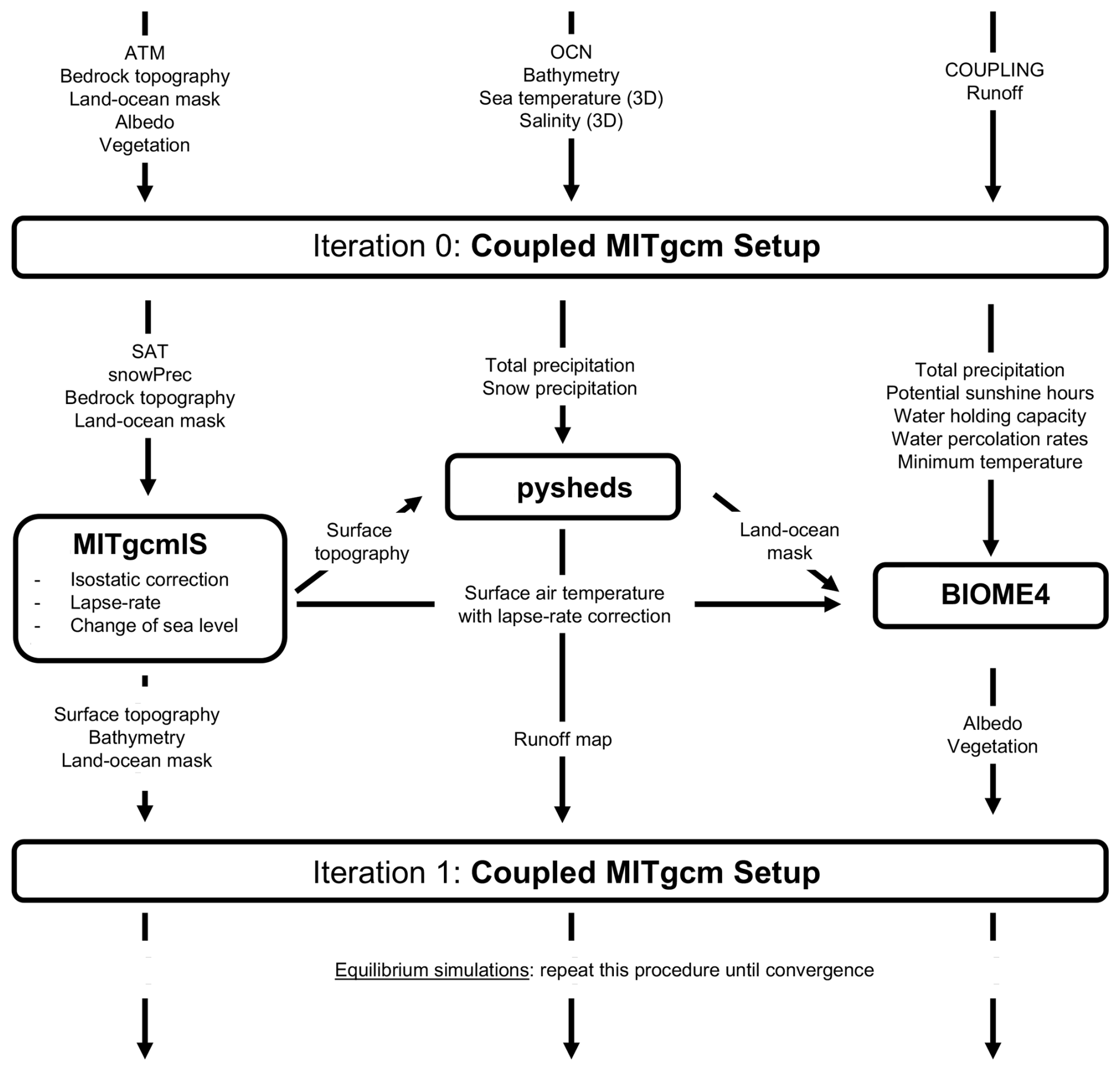
A first simulation is run until the Coupled MITgcm Setup has reached a steady state, defined by having a surface energy balance $F_{\mathrm{s}}<\mathrm{0.2}\mathrm{W}{\mathrm{m}}^{-\mathrm{2}}$ (usually several thousands of simulated years are required). Afterwards, additional 30 year are run with monthly frequency for the variables required by BIOME4, and with daily frequency for the variables required by MITgcmIS.

At this point, the offline coupling workflow can start. Before running the ice sheet model, the following corrections are required. For representing an advancing ice flow over shallow ocean, we mimic this process as follows: if the sea ice thickness is equal to the ocean depth (up to a depth of −20 m), the ocean point becomes a land point and hence the ice sheet can develop on it. Then, the corrected topography file is given as an input to the ice-sheet model, together with daily MITgcm outputs per grid cell for SAT and snow precipitation, which are used to calculate ablation and accumulation rates, respectively. MITgcmIS is run for 40–100×10³ years, during which the isostatic adjustment is calculated and the lapse rate from the previous convergence step is used, until the ice sheet reaches a steady state (MacAyeal, 1997). Sea level correction and salt compensation (Sect. 2.4.3) are included at this stage, giving rise to new topography (including ice sheet height), mask and bathymetry files. Afterwards, pysheds is applied using the mask and the topography, closing lakes and small passages if necessary, and giving a new runoff map as output.

Finally, the vegetation model is run based on the new files. The outputs needed from MITgcm and the ice-sheet model (namely, precipitation, SAT and sunshine) are converted on a latitude/longitude grid and then given to the BIOME4 model. The equilibrium biome distribution is converted in new files for vegetation fraction and surface albedo using the values reported in Haywood et al. (2010). Due to the coordinate change, some land and ocean points can be inverted on the cubed-sphere grid. Hence, a vegetation fraction equal to 0 and an albedo value equal to the default water value of 0.07 are assigned to new ocean points on the CS grid, while the value of the closest land point is assigned to new land points.

Before running a second iteration, salinity and sea temperature at all ocean levels are averaged over the last 30 yr to generate new input files for the Coupled MITgcm Setup. Then, these files, along with the new vegetation fraction, albedo, topography, bathymetry, runoff and mask files, are given back to the Coupled MITgcm Setup to run the whole coupling process at least twice, so that the GCM has time to adjust to the new input files. Convergence is considered achieved when less than 10 % of the land points experience a change in biome distribution and total ice sheet volume. Moreover, the Coupled MITgcm simulation needs to have a surface energy imbalance $F_{\mathrm{s}}<\mathrm{0.2}\mathrm{W}{\mathrm{m}}^{-\mathrm{2}}$, corresponding to extremely low drifts in both the global ocean temperature and the surface air temperature. The whole procedure forms the BIG-MITgcm simulation tool, which thus describes the climatic steady state, including those components with a slow response, like deep-ocean dynamics, vegetation and ice sheets.

3 Experimental setup

3.1 Comparison with data and CMIP models

To assess the performance of our climate framework BIG-MITgcm, we run three simulations. The first one, denoted as run1, is the pre-industrial simulation at 280 ppm starting from an input map of land elevation in the absence of ice. This simulation will be assessed against two CMIP6 models, as there is a lack of observational data for this period. The second simulation (run2), which corresponds to the 1979–2009 period with an average CO₂ concentration of 360 ppm (Lan et al., 2025), is started from the run1 steady state by applying a constant increase of CO₂ of 1 ppm yr⁻¹ for 80 year and keeping the ice sheet fixed. This run is evaluated against reanalysis and observational data. Finally, a third simulation (run3) is run using the Coupled MITgcm Setup at 280 ppm starting from ETOPO2 (thus, including present-day ice sheets) and the vegetation cover obtained in run1. Comparing run1 and run3 helps evaluate the ability of BIG-MITgcm to grow plausible ice sheets.

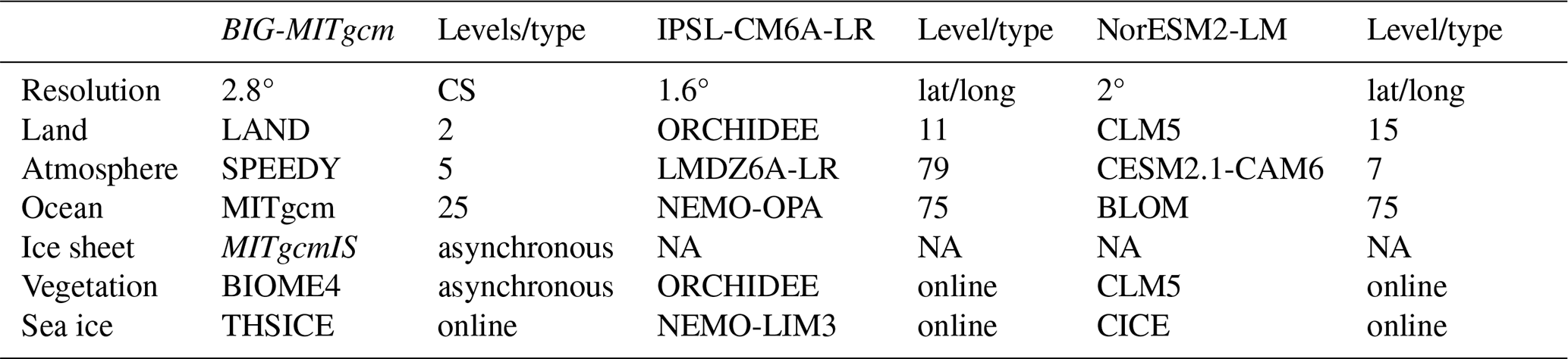
More specifically, for assessing the pre-industrial run at 280 ppm, we use the output data from the IPSL-CM6A-LR model (Boucher et al., 2018) and the NorESM2-LM model (Seland et al., 2020) using the piControl dataset (Eyring et al., 2016). We chose these two CMIP models because they include dynamical vegetation (see Table 1). For the second run at 360 ppm, we compare our data with the following datasets: ERA5 (Hersbach et al., 2023) for the atmosphere, OSRA5 (Copernicus Climate Change Service, 2021) for ocean diagnostics, MODIS for the vegetation, BedMachine for the surface elevation of Greenland and Antarctica (Morlighem et al., 2022; Morlighem, 2022), RAPID observations for the Atlantic Meridional Overturning Circulation (AMOC) profile (Moat et al., 2025), and the Sea Ice index for the sea ice extent (Fetterer et al., 2002).

Table 1 Models description: module names with corresponding number of vertical levels or type of coupling.

Five iterations of the procedure illustrated in Fig. 1 were necessary to reach convergence in run1. The last 30 years of the fifth iteration are used for diagnostics. To be consistent in comparisons, all diagnostics are converted to the same longitude-latitude coordinate system with a spatial resolution of 2°×2°.

The outputs were treated using Matlab version 2023b and the figures were made using python. The MITgcm took approximately 1500 simulated years per week to reach equilibrium using 25 processors for each iteration. BIOME4 and pysheds run in less than 5 min on a desktop computer. MITgcmIS needs around 1 h of CPU time for 40 thousand years due to the daily stepping of Eqs. (6)–(7) for all ice-covered points.

3.2 BIG-MITgcm initial conditions

To start the first run of our simulations, it is necessary to provide initial conditions that are representative of the present-day climate. The three-dimensional distributions of sea potential temperature and salinity are derived from the Levitus World Ocean Atlas (Levitus, 1982). Orbital forcing is prescribed at present-day values, with a solar constant of 1365.4 W m⁻² and obliquity of 23.45°. Topography (including ice sheets and glaciers), bathymetry and the corresponding files are taken from the ETOPO2 dataset (ETOPO2, 2006) with a resolution of 2 arcminutes. Annual mean values of bare-surface albedos (in the absence of snow or ice) and fraction of land-surface covered by vegetation are the same as those used in Molteni (2003) and derived from the ERA dataset. Interpolation and smoothing are applied to convert these maps to the resolution of the MITgcm CS32 grid (Ragon, 2024).

In order to assess the ability of MITgcmIS to correctly generate the ice sheets, we need to provide an input map of land elevation in the absence of ice. This map was generated using the BedMachine dataset that is part of the MEaSUREs program of NASA (Morlighem, 2022; Morlighem et al., 2022), with the addition of an isostatic correction as in Paxman et al. (2022a) for Antarctica and Greenland. The BedMachine dataset provides a density-corrected satellite-based DEM of the ice sheet surface, as well as a data-constrained estimate of bedrock elevation and a mask for identifying the different parts of the ice sheets. There are two separate products for Antarctica (Morlighem, 2022) and Greenland (Morlighem et al., 2022), respectively. The surface elevation of the ice sheets are used to assess the performance of MITgcmIS, while bedrock elevations with isostatic adjustment are used as initial boundary conditions, as shown in Fig. 2. Note that, regarding paleoclimate simulations, PANALESIS or other reconstructions directly provide unloaded bedrock elevations.

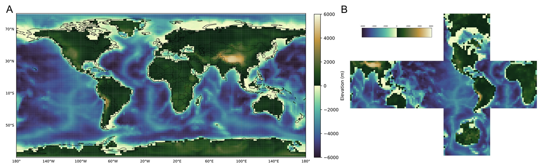
Figure 2 Bedrock topography (with isostatic adjustment) and bathymetry used as initial boundary conditions in the pre-industrial run at 280 ppm (run1) on the latitude-longitude grid (A) and on the cubed-sphere grid (B).

Finally, it is important to also describe the tuning procedure. In order to obtain pre-industrial conditions at 280 ppm, once all the albedo values for vegetation cover, snow and ice have been fixed and set to values within observational ranges, we tune the relative humidity threshold for the formation of low clouds (a parameter denoted as RHCL2 in SPEEDY) so that the average global SAT becomes approximately equal to the observed value of 13.7 °C (NOAA National Centers for Environmental Information, 2024). The adjusted value, RHCL2=0.7727, is applied to all simulations. Moreover, the coefficient a in Glen's law, which in our simulations is assumed to be constant (see Eq. 2) and governs the ice sheet formation, is determined as follows.

Evaluating the surface mass balance produced for Antarctica in our setup is necessary to calibrate the Glen's law parameter using the total ice sheet volume. The reason is that the volume is strongly sensitive to both the net surface mass balance and the Glen's law coefficient; without a good estimate of the surface mass balance, the correct volume can be achieved for the wrong reasons. The surface mass balance of Antarctica is estimated by the Coupled MITgcm Setup started from the present-day ice sheets (ETOPO2), and turns out to be approximately 1500 Gt yr⁻¹. This value can be compared with the ensemble mean obtained from a comparison of Regional Climate Models (RCMs) in Mottram et al. (2021). In that study, the ensemble mean over the grounded ice sheet is estimated at 2073±306 Gt yr⁻¹. Although the value obtained in our simulation is lower than this ensemble mean, as well as lower than the values obtained by all individual models in that comparison, it is important to consider that the spatial interpolation and smoothing applied to obtain 2.8° resolution in our simulations (Ragon, 2024) implies a different representation of the Antarctic continent compared to models with finer resolutions (25–50 km). Additionally, there are known limitations in the representation of snow processes in the land module, as discussed in Sect. 2.4. Therefore, even if our value is lower than those obtained from RCMs, it remains within the same order of magnitude. Using this value for the surface mass balance, we apply our ice sheet model MITgcmIS (which always starts from the bedrock and isostatic adjusted topography) with a range of a values. This yields different Antarctic volumes (Table A1), while maintaining a similar surface elevation profile. We selected $a=\mathrm{0.6}\times {\mathrm{10}}^{-\mathrm{15}}$ ${\mathrm{Pa}}^{-\mathrm{3}}{\mathrm{yr}}^{-\mathrm{1}}$ as a compromise, as it produces a volume within 10 % of the observed value and surface elevations consistent with observations.

4 Results

4.1 BIG-MITgcm evaluation

To evaluate if our coupling setup correctly reproduces the modern Earth climate, we examined several diagnostics of the dynamical behavior of atmosphere, ocean, vegetation and cryosphere.

4.1.1 Atmosphere

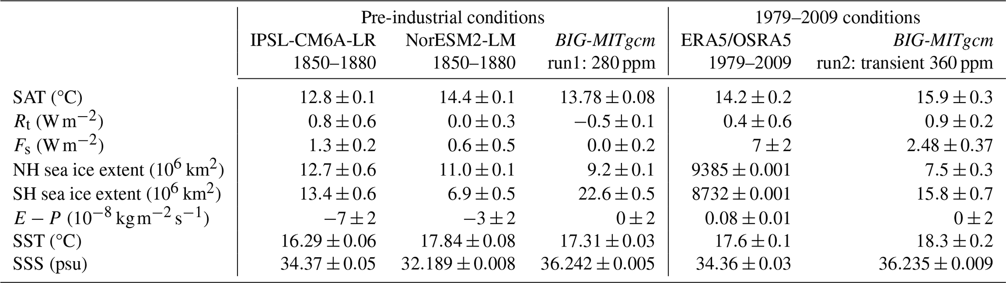
In Table 2 global mean values of the relevant variables, calculated from the last 30 simulated years, are listed, together with the reanalysis data and the climatology values from the two CMIP models. The global mean SAT of 13.78 °C in run1 is intermediate between the two CMIP values, and close to the measured pre-industrial (1850 year) value of 13.7 °C (NOAA National Centers for Environmental Information, 2024) because of our tuning procedure. However, the global mean SAT of 15.9 °C for the 1979–2009 period in run2 is larger than the ERA5 value. This depends on the Equilibrium Climate Sensitivity (ECS), which is around 5 °C in our model, i.e. in the highest range of CMIP6 values (Nijsse et al., 2020; Zelinka et al., 2020).

Table 2 Global annual mean values averaged over the last 30 years, and associated standard deviations derived from interannual variability. The acronyms in the table are: surface air temperature (SAT), top-of-the-atmosphere budget (R_t), ocean surface budget (F_s), Northern Hemisphere (NH), Southern Hemisphere (SH), evaporation minus precipitation (E−P), sea surface temperature (SST) and sea surface salinity (SSS).

More in detail, if we look at the SAT zonal profiles shown in Fig. 3 (first column), we can make common remarks for the two runs concerning the polar regions. The overall behaviour is well reproduced in our simulations, except the temperature around 60S, which is approximately 10 °C lower in BIG-MITgcm compared to the CMIP6 models and the ERA5 values, as also shown in Fig. A1. This is due to the Southern Hemisphere sea ice extent, which is higher than in CMIP models and observations, probably because our setup does not include dynamical but only thermodynamical effects. This is confirmed by run3, showing the same behavior. Figure A1 also shows that SAT over ice sheets is higher than in CMIP models and observations. This can be due to the coarser resolution of the Coupled MITgcm Setup (2.8°), which underestimates the elevation of Antarctica and Greenland, hence giving higher temperatures than observations and CMIP models, where the ice sheet elevation is fixed to observed values.

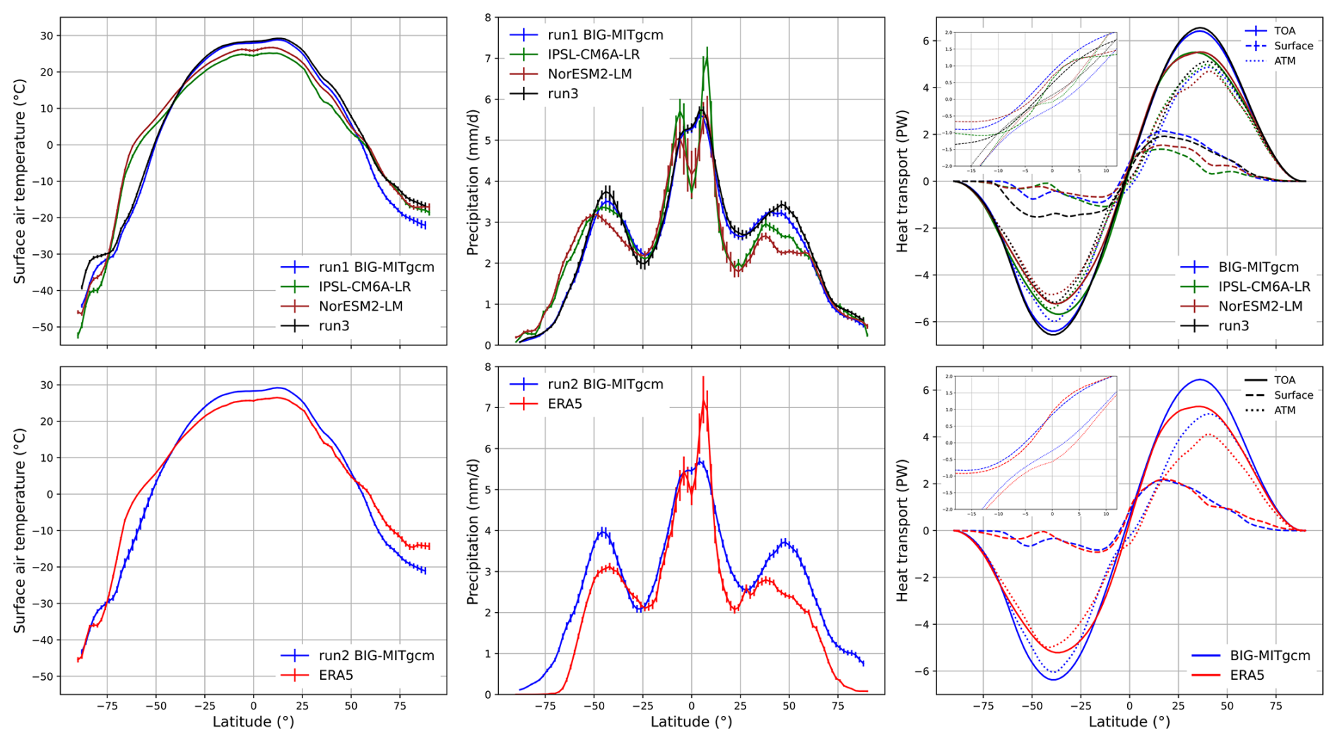
Figure 3 Zonal profile of the surface air temperature (first column), precipitation (second column) and the heat transport (third column). The first line represents the simulations that were run under pre-industrial conditions (280 ppm) and the second line under the 1979–2009 conditions. For the pre-industrial conditions, BIG-MITgcm run1 (blue), IPSL-CM6A-LR (green), NorESM2-LM (dark red), and run3 (black) data are plotted. For the 1979–2009 conditions, BIG-MITgcm run2 (blue) and ERA5 (red) data are plotted. The heat transport panels contain the top-of-the-atmosphere (TOA, solid lines), the atmosphere (ATM, dotted lines) and the surface (dashed lines) components. The inset panel for the heat transport is a zoom around the equatorial region.

Another important feature to be checked regarding the atmosphere dynamics is the model capability to correctly reproduce the Hadley cells, as shown in Fig. 4. In run2, our model gives rise to a weaker positive overturning cell near the Equator, as also seen by Ruggieri et al. (2024) where the 8-layer SPEEDY module is coupled with the NEMO ocean. However, from run1 we see that the positive overturning cells reconstructed by NorESM2-LM are similarly weak, despite a number of vertical layers in the atmosphere that is larger than the 5 layers in SPEEDY-MITgcm. In run1, SPEEDY gives cells with similar extent as the IPSL-CM6A-LR model, which has a state-of-the-art atmospheric module with 75 levels, while there is an additional positive south polar cell in the NorESM2-LM model. The lower branch of the positive Hadley cell is less intense than that in IPSL-CM6A-LR and ERA5. This feature has direct consequences on southward transport of water mass in the tropics, as shown in Fig. A2, which in our setup is indeed weaker than observations and CMIP models. In contrast, the transport towards the southern polar region turns out to be larger in our simulations due to the comparatively intense Ferrel cell in the Southern Hemisphere. In addition, the mean zonal wind in our simulations, shown in Fig. A3, agrees with ERA5 and the two CMIP models, with a slightly lower intensity of the jet stream in the Northern Hemisphere. Despite these limitations, it is important to note that the total water mass E−P shows only a small imbalance in our simulations with respect to the control runs of the two CMIP models, as reported in Table 2.

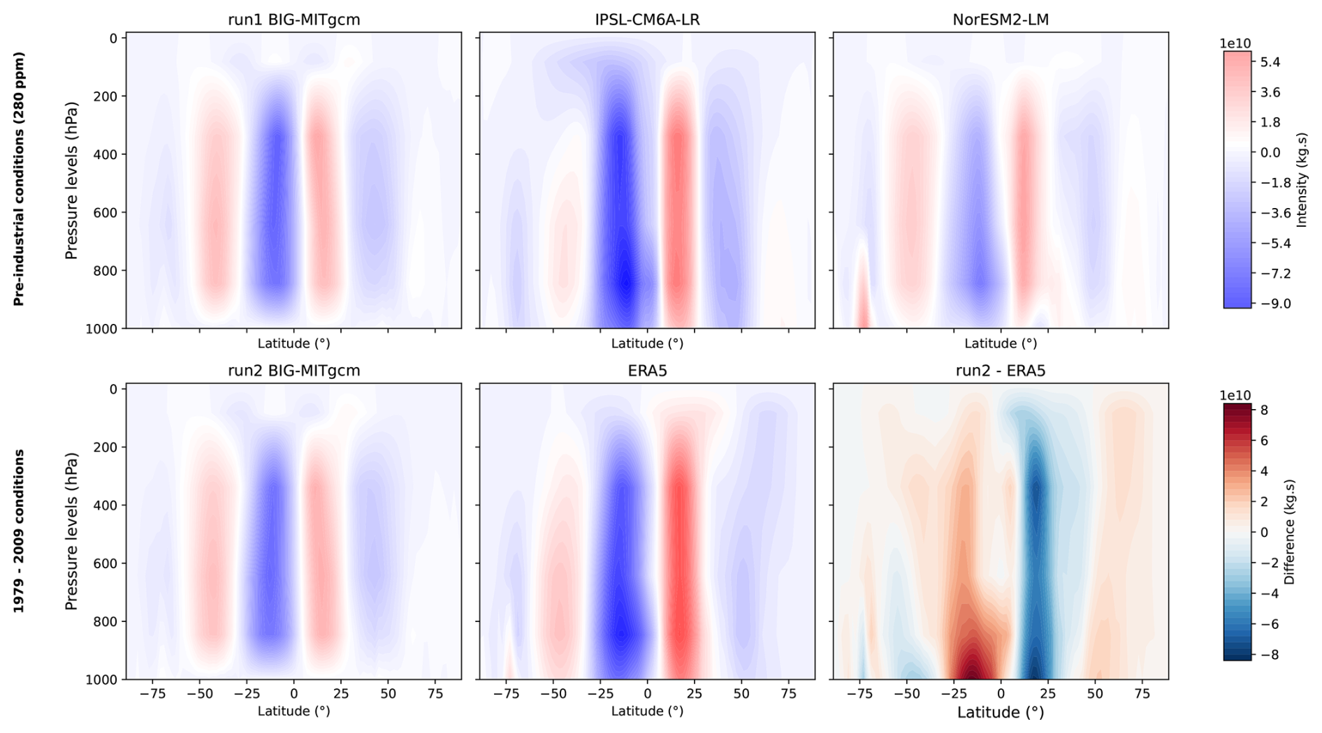
Figure 4 Atmospheric overturning cells for the pre-industrial conditions (first line) and for the 1979–2009 conditions (second line). For the pre-industrial conditions, BIG-MITgcm run1, IPSL-CM6A-LR and NorESM2-LM data are plotted in this respective order. For the 1979–2009 conditions, BIG-MITgcm run2, ERA5 data and the difference between the two are plotted, respectively.

As we can see in Fig. 3 (second column), while the precipitation peak at the ITCZ is correctly reproduced in our simulations, at a mean latitude of approximately 6° N (Marshall et al., 2014) that corresponds to the ascending branch of the Hadley cells, the precipitation intensity at ITCZ is underestimated due to weak Hadley overturning cells. In addition, our simulations do not capture the decrease in precipitation intensity at the Equator, as also observed in Ruggieri et al. (2024). The precipitation is in general overestimated in BIG-MITgcm with respect to observations in the extratropics, with peaks occurring at higher latitudes. However, the SPEEDY module captures the overall precipitation pattern in both runs (see Fig. A4), with localised maximum anomalies of around 5 mm d⁻¹ in the equatorial region.

The heat transport at the top of the atmosphere (TOA) in Fig. 3 (third column, solid lines) shows that BIG-MITgcm closely follows the overall pattern in both runs, except for sligthly stronger total heat transport at approximately 40° S and 40° N. Across the Equator, the atmospheric heat transport (dotted lines) is southward in our simulations and in ERA5, correctly compensating for the northward ocean heat transport driven by the AMOC, as described in Marshall et al. (2014). In contrast, the CMIP models do not show this compensation across the Equator despite their finer vertical resolution in the atmosphere, as can be seen in the inset of Fig. 3 (third column). Moreover, as shown in Table 2, the energy budget R_t at TOA is almost closed in BIG-MITgcm run1 and within the range of CMIP models (Lembo et al., 2019). In run2, the TOA imbalance increases due to forcing conditions.

4.1.2 Ocean

In order to assess the capacity of BIG-MITgcm to correctly represent the ocean dynamics, we looked at the sea surface temperature (SST) and salinity (SSS), the sea ice extent, the water-mass budget, the AMOC profile and the heat transport at the surface.

As shown in Table 2, SST in BIG-MITgcm run1 is in between the two CMIP models, whereas it is higher than in OSRA5 being consistent with SAT. Sea ice extent in our run1 simulation is lower in the Northern Hemisphere (NH) than in the Southern Hemisphere (SH), in contrast to NorESM2-LM results. Note that the NorESM2-LM model simulates a pre-industrial climate with less SH sea ice (with an extent of 6.9×10⁶ km²) compared to ERA5 (with approximately 8.7×10⁶ km²), even though ERA5 reflects a climate state with a higher atmospheric CO₂ content.

For run2, the values of sea ice extent in BIG-MITgcm differ from those in ERA5 (lower in the Northern Hemisphere and higher in the Southern Hemisphere), due to the starting values obtained in the pre-industrial run. However, we observe that the sea ice extent obtained in our simulations, shown in Fig. A5, is in good agreement with that in Ruggieri et al. (2024), obtained with SPEEDY-NEMO for the period 1979–2014.

Our two simulations show a reduction in the sea ice extent with increasing atmospheric CO₂ concentrations. The total extent of sea ice in our run1 simulation is larger than in NorESM2-LM, which explains a higher value of salt concentration. It is comparable to that of IPSL-CM6A-LR, which, however, shows an imbalance in the water budget of $E-P=-\mathrm{7}\times {\mathrm{10}}^{-\mathrm{8}}$ $\mathrm{kg}{\mathrm{m}}^{-\mathrm{2}}{\mathrm{s}}^{-\mathrm{1}}$ and a slightly lower value of salinity.

The ocean heat transport (OHT) in Fig. 3 (third column, dashed lines) shows a larger amount of heat towards the northern polar region compared to CMIP models, explaining why our setup produces less sea ice there. The bulk of the OHT is dominated by the Ekman transport in the subtropical gyres. As mentioned before, the AMOC effect is to increase heat transport across the Equator (Marshall et al., 2014), which is of around 0.7 PW in all models. It is important to note that the surface energy imbalance F_s of run1 is very low ($\left|F_{\mathrm{s}}\right|\le \mathrm{0.1}\mathrm{W}{\mathrm{m}}^{-\mathrm{2}}$, see Table 2), because it is run close to equilibrium. In contrast, $F_{\mathrm{s}}=\mathrm{2.48}\mathrm{W}{\mathrm{m}}^{-\mathrm{2}}$ in run2 and $F_{\mathrm{s}}=\mathrm{7}\mathrm{W}{\mathrm{m}}^{-\mathrm{2}}$ in the observations, reflecting forced conditions. Although they represent control runs, the two CMIP simulations exhibit values larger than 0.1 W m⁻², indicating that they are not fully equilibrated.

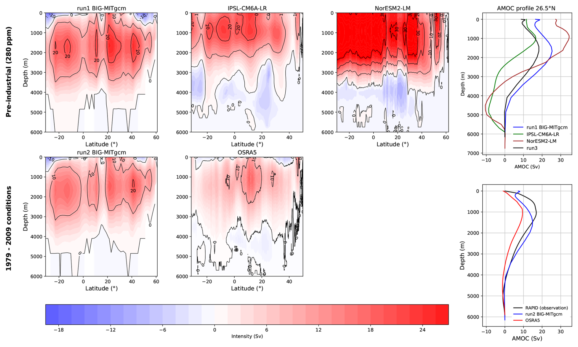
Figure 5 Atlantic meridional overturning circulation (AMOC) intensity for the pre-industrial conditions (first line) and the 1979–2009 conditions (second line). The coloured plots represent the intensity of the overturning and the two most right panels represent the AMOC intensity profile at 26.5° N (as in the RAPID measurement). For the pre-industrial conditions, BIG-MITgcm run1, IPSL-CM6A-LR and NorESM2-LM intensity data are plotted (run3 is also added in the 26.5° N profile). For the 1979–2009 conditions, BIG-MITgcm run2 and OSRA5 data are plotted.

As shown in Fig. 5, the AMOC produced by our coupled setup for run1 has a clockwise (positive) overturning cell with intensity comparable to the cell obtained by IPSL-CM6A-LR, which however develops at lower depths. The positive overturning cell in NorESM2-LM has a higher intensity than both BIG-MITgcm and IPSL-CM6A-LR. For run2, the AMOC intensity produced by OSRA5 exhibits a maximum at the Tropics, while in our coupled setup there are several regions of high intensity. In both, there is a weak anticlockwise (negative) overturning cell at depths higher than 4 km. Right panels in Fig. 5 show vertical profiles at 26.5° N of the AMOC streamfunction. The two blue curves correspond to the BIG-MITgcm simulations and show that there is a decrease in the intensity of the AMOC positive cell as the CO₂ concentration increases. This behavior is expected (Caesar et al., 2018) and demonstrates the ability of BIG-MITgcm to produce consistent results. It is important to note that the two CMIP models exhibit strong negative values around 4500 m depth that do not appear in the observations. A similar pattern is also observed in another class of CMIP models described in Valdes et al. (2017), even in present-day simulations. However, BIG-MITgcm shows the maximum of the positive cell around 1500 m, whereas it should be around 1000 m according to the RAPID measurements. This discrepancy may be related to the fact that the MITgcm ocean module includes only 25 vertical levels, compared to 75 in the two CMIP models.

4.1.3 Vegetation

In this section, we evaluate the capacity of the coupled system to correctly reproduce the present-day vegetation and we assess its performance against models with dynamical vegetation.

As shown in Fig. 6C, BIG-MITgcm run2 gives rise to a good representation of the major biomes. Run2 displays the boreal forest, which, following the biome classification used in Kaplan et al. (2003) and Haywood et al. (2010), corresponds to cool mixed forests, evergreen and deciduous taiga (see the legend in Fig. 6C). It also displays the Amazon rainforest by returning the tropical evergreen forest biome, and the desert biome (Norby et al., 2005), although the latter is smaller than in observations. This is directly linked to the excess of precipitation produced by the SPEEDY module in North Africa (Fig. A4).

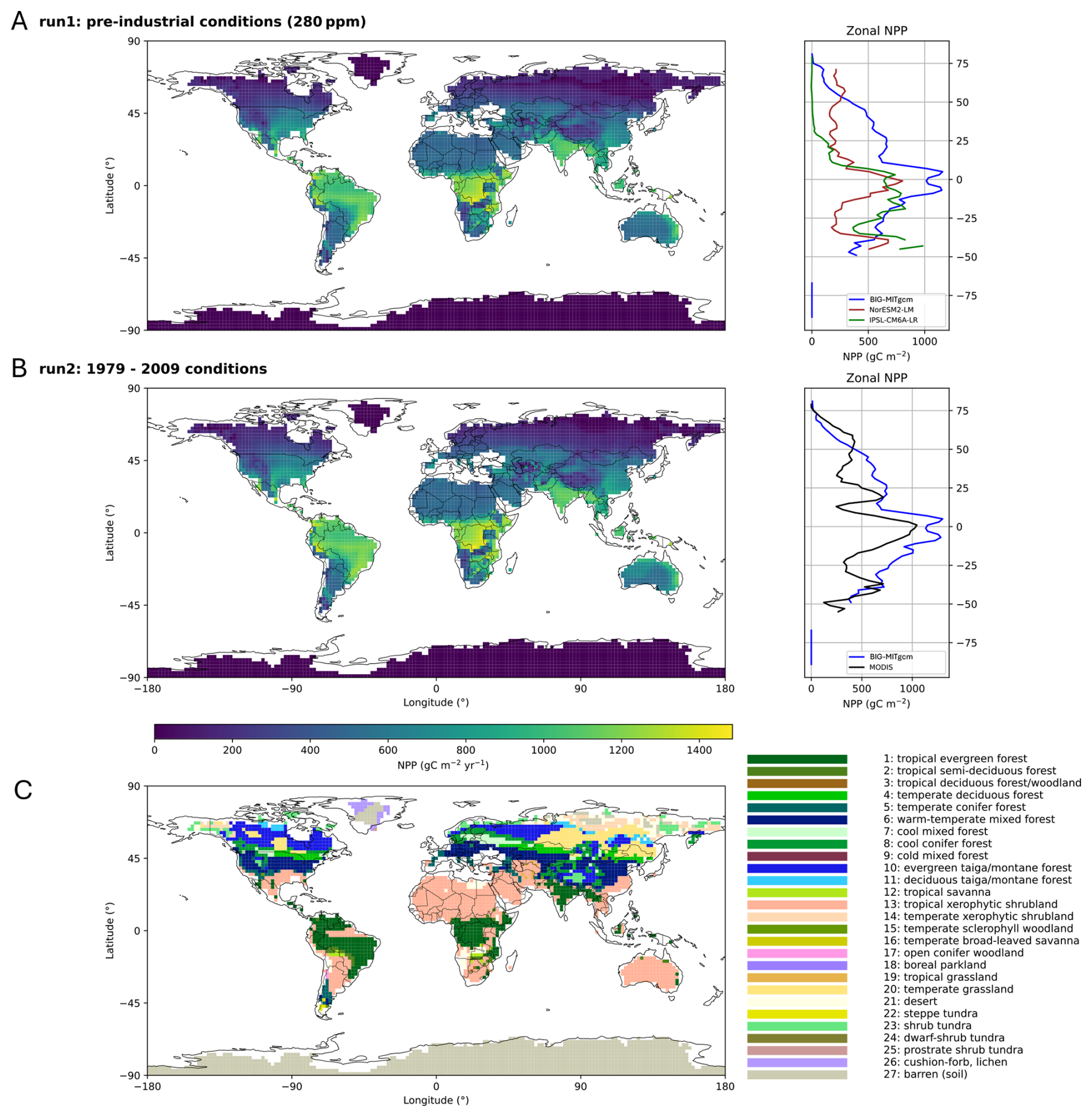
Figure 6 Net primary productivity (NPP) for the pre-industrial conditions for BIG-MITgcm run1 (panel A) and 1979–2009 conditions for BIG-MITgcm run2 (panel B), biome distribution for the 1979–2009 conditions for BIG-MITgcm run2 (panel C), with the corresponding colormap biome designation. The right most panels are the zonal profiles of the NPP distribution in the pre-industrial conditions for BIG-MITgcm, IPSL-CM6A-LR and NorESM2-LM, and in the 1979–2009 conditions for BIG-MITgcm run2 and MODIS.

Maps and zonal profiles of the Net Primary Production (NPP) for run1 and run2 are shown in Fig. 6A and B. The zonal profiles are compared to those of CMIP models and the MODIS dataset. Our simulations reproduce the general pattern by correctly displaying an increase in the equatorial region. However, they fail to capture the decrease at 10 and −25° latitude, as shown by MODIS. It is important to note that there is a difference in NPP intensity between run1 and run2. This is mainly explained by the increase of CO₂ concentration, precipitation and temperature, as shown in Fig. 3 (first and second columns). The two CMIP models show different behaviors. NorESM2-LM captures quite well the decrease at 10 and −25°, as well as the increase in the equatorial region, despite lower intensities than MODIS. IPSL-CM6A-LR does not show vegetation at latitudes higher than 25° N, as ORCHIDEE does not include high-latitude biomes such as tundra (Dinh et al., 2024). The two dynamical vegetation models do not capture all the trends in the NPP pattern, even with more sophisticated land modules than the one used in our setup. This is confirmed by the correlation analysis shown in Fig. A6. The correlation coefficient r is close to 0.8 and the slope value is close to 1 when the results of run2 are plotted against MODIS, confirming a broad agreement with observations. The correlations of the results of run1 against the two CMIP models are around 0.6. This emphasizes that, even without online dynamical vegetation, our setup successfully captures global-scale vegetation features.

4.1.4 Ice sheet

The performance of MITgcmIS is evaluated against present-day observations using the BedMachine datasets. Since there are no observational data available for the pre-industrial period, and the two CMIP models do not include dynamical ice sheets, BIG-MITgcm run 1 is assessed using present-day observations. We also compare the resulting climate in run1 with that obtained in run3 (started from ETOPO2, i.e. fixed present-day ice sheets, and same vegetation as in run1). We find that the resulting climatic attractors are essentially the same, with very small differences in terms of temperature and precipitation, as shown in Fig. A7, and limited differences in the zonal profiles (see Figs. 3 and 5), demonstrating the ability of our procedure to reconstruct first-order processes in ice sheets.

The ice sheets obtained in run1 are shown in Fig. 7. The total volume is 24.5×10⁶ km³, of which 21.0×10⁶ km³ in Antarctica (due to the tuning procedure, Sect. 3.2) and 3.5×10⁶ km³ in Greenland. Hence, in run1 the ice sheet volume is of the same order as the observed volume (22.9×10⁶ km³ for the Antarctica ice sheet and 28.0×10⁶ km³ for the observed total ice sheet volume, after smoothing on the same 32×32 cubed-sphere grid) (Morlighem et al., 2022; Morlighem, 2022). Other glaciers (in Alaska, Canada, India, etc), with a global glacier volume of around 1.6×10⁵ km³ (Farinotti et al., 2019), are not captured by our model due to its coarse resolution.

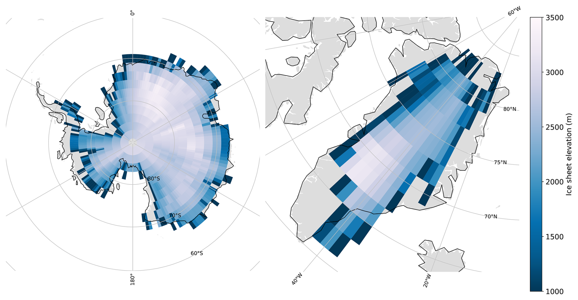
Figure 7 Ice sheet elevation for Antarctica in ESPG:3031 projection (left panel) and Greenland in ESPG:3413 projection (right panel) obtained from BIG-MITgcm run1.

This overall agreement with observations (BedMachine dataset) is confirmed in statistically significant Pearson correlation coefficients of 0.76 and 0.80 for the surface elevation of both ice sheets and Antarctica only, respectively, as shown in Fig. A8. However, the slope values of 0.33 and 0.35 for both ice sheets and Antarctica only, respectively, are lower than 1. This means that the model tends to underestimate the largest ice sheet heights and to overestimate the smallest ones on the edges. This pattern is evident in Fig. A9, particularly in West Antarctica. In contrast, conclusions about Greenland are more uncertain due to the limited pixel coverage. Overall, we observe that Antarctica in MITgcmIS agrees more closely with observations than Greenland.

If we examine the histograms in the right panel of Fig. A9, we observe that they support the conclusions discussed above. The excess accumulation in West Antarctica is also reported in Xie et al. (2022), which uses an ice sheet model of similar complexity. In addition, analogous biases in ice thickness are also observed in more sophisticated models, such as in Quiquet et al. (2018), which underestimates the ice thickness in central Antarctica of around 300–400 m. The fact that MITgcmIS does not correctly capture the peak of ice sheet elevation in central Antarctica can be attributed to the model's coarse spatial resolution, confirming the role played by spatial resolution in ice sheet models (Rückamp et al., 2020). In addition, it is important to consider uncertainties related to measurements of bedrock elevation, isostatic adjustment, and ice sheet thickness. Nevertheless, we can conclude that our model reproduces the first-order characteristics of the ice sheets reasonably well.

4.1.5 Runoff

The final topography obtained in run1 is shown in Fig. 8A. The topography includes the ice sheets formed by iterating the asynchronous coupling procedure five times (Fig. 1). By applying pysheds to this topography, the drainage basins and the corresponding main rivers are identified, resulting in the runoff routing map shown in Fig. 8B. In this way, each land point is associated with an ocean point corresponding to the revelant river mouth. The main river paths can be clearly recognised, such as the Amazon, Congo, Nile or Yangtze rivers.

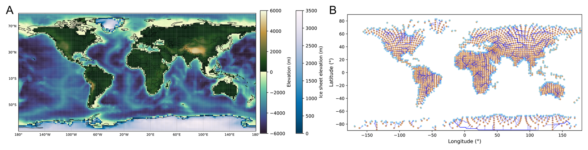
Figure 8 Topography with ice sheet elevation obtained as an output from BIG-MITgcm run1 (panel A) and the corresponding runoff routing map (panel B).

4.2 The Permian-Triassic case

We now demonstrate how the asynchronous procedure can be applied to a very different continental configuration. As an example, we consider the Permian-Triassic bedrock paleogeography as reconstructed by PANALESIS (Vérard, 2019). Three alternative climatic steady states have been identified for this paleogeography by Ragon et al. (2024), with mean surface air temperatures (SAT) higher than present-day values. However, the so-called cold state, with an average SAT of around 17 °C and a meridional overturning circulation characterised by a negative cell (i.e. flowing from north to south at the surface), corresponds to climate conditions where a small ice cap can develop in the Northern Hemisphere. Therefore, we applied our procedure to investigate this possibility.

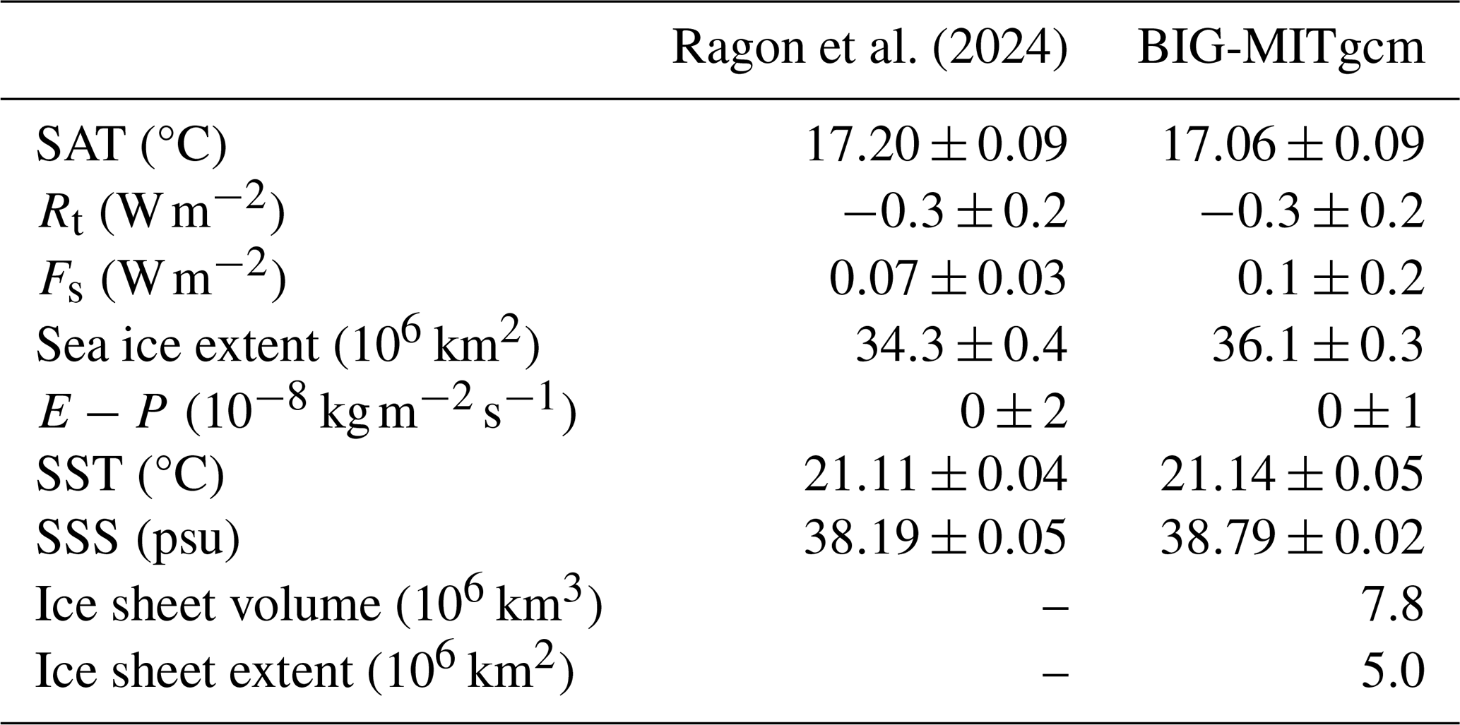
We find that a small ice cap can indeed develop in the Northern Hemisphere in the cold state, as shown in the resulting topography in Fig. 9A. The associated runoff routing map is also shown in Fig. 9B. Global annual values of the main climatic variables, listed in Table 3, fall within the same range as those reported by Ragon et al. (2024), with slightly lower SAT and higher sea ice extent, indicating that this climatic state can be represented by the same attractor. The ice sheet extends in the north polar region with a volume of 7.8×10⁶ km³, corresponding to approximately −20 m of sea-level change relative to a climate state without ice sheets, and −65 m relative to the present-day value. Interestingly, this value falls within the range of eustatic variations in the Early Triassic reconstructed by global stratigraphic data (Haq, 2018; Simmons et al., 2020).

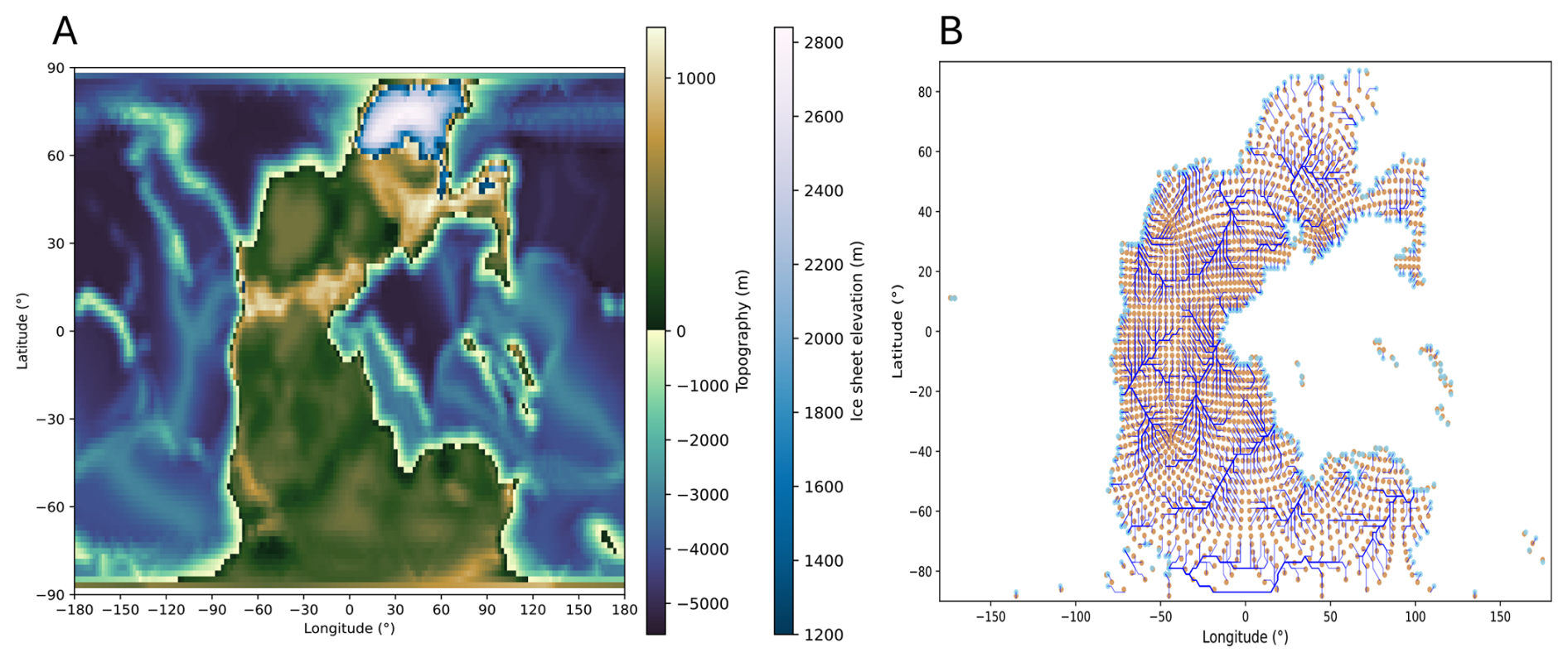
Figure 9 Permian-Triassic topography from the PANALESIS reconstruction with ice sheet elevation obtained using BIG-MITgcm (panel A). The bedrock elevation used to start the simulation can be found in Ragon et al. (2024). Runoff routing map for the corresponding topography (panel B).

Table 3 Global annual mean values averaged over the last 30 years, and associated standard deviations derived from interannual variability. The acronyms in the table are: surface air temperature (SAT), top-of-the-atmosphere budget (R_t), ocean surface budget (F_s), evaporation minus precipitation (E−P), sea surface temperature (SST) and sea surface salinity (SSS).

Regarding the vegetation cover, the main differences in NPP distribution relative to Ragon et al. (2024) occur at high latitudes, as shown in Fig. 10, due to the equatorward migration of temperate forests and the disappearance of tundra in regions covered by the ice sheet.

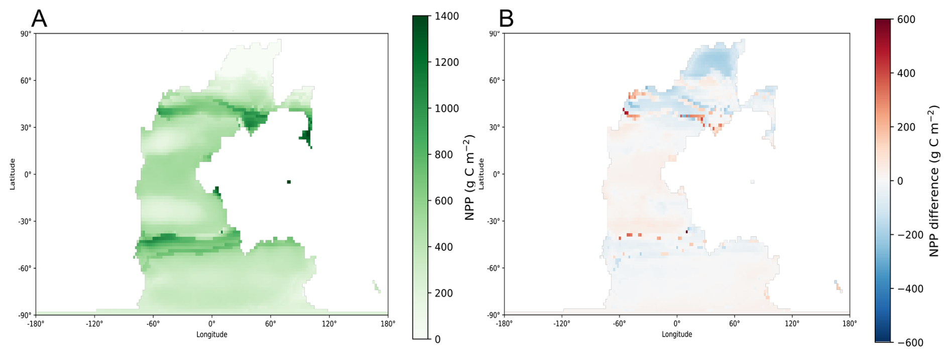
Figure 10 NPP distribution map obtained with BIG-MITgcm (panel A) and the difference with the cold state in Ragon et al. (2024) (panel B).

5 Future developments

In this paper, we have described how the implemented asynchronous coupling framework successfully reproduces the large-scale climate and its major components, giving results comparable to those of two CMIP6 models for the pre-industrial climate, and demonstrating its capability to represent deep-time climates. However, further improvements are possible, some of which we discuss below.

The atmospheric module is currently based on a previous version of SPEEDY with five vertical levels, while a newer version with eight levels is now available (Kucharski et al., 2013). This updated version has recently been coupled with the NEMO ocean model (Ruggieri et al., 2024), providing a good representation of both climatology and the main modes of internal variability. A further improvement would be to directly implement the asynchronous coupling with BIOME4 on the MITgcm cubed-sphere grid, thereby eliminating interpolation errors, as discussed in Sect. 2.6.

Regarding the ice sheet model, we plan to provide the option of performing both online and offline coupling with the MITgcm dynamical kernel. This upgrade requires an enhancement of the land module within MITgcm. While incorporating a detailed land surface scheme, such as the one used in the JULES model (Wiltshire et al., 2020) would constitute a major improvement, we plan to follow a different approach, as only selected processes need to be represented at coarse spatial resolutions. As mentioned in the Methods section, the current two-layer land module in MITgcm lacks representations of processes such as heat conduction in snow, meltwater refreezing and retention, and snow compaction. All of these can significantly affect the ablation and accumulation in the surface mass balance, which is currently underestimated in our simulations. The use of the open-source snowpack model described in Essery (2015) could be a viable option. In future iterations of MITgcmIS, sliding and basal heat balance could easily be implemented – this would allow study of nonlinear processes that occur over continental and millennial scales, such as binge-purge oscillations (MacAyeal, 1993). Furthermore, incorporating a dynamical ice sheet model would lead to a more consistent energy budget across the different model components. However, due to the slow temporal evolution of ice sheets starting from bedrock conditions, a spin-up phase using offline coupling will always be necessary, since the Coupled MITgcm Setup cannot be run on timescales of hundreds of thousands of years due to computational costs.

6 Conclusions

In summary, the BIG-MITgcm coupled setup provides a good representation of large-scale features of the present-day climate with reasonably low computational costs. Atmosphere and ocean dynamics broadly agree with observations, giving a model performance comparable to CMIP6-class models. Coupling with the BIOME4 vegetation model reproduces the main biomes, with results similar to those obtained using CMIP6 models with dynamical vegetation. Moreover, the vegetation cover obtained with BIG-MITgcm exhibits coherent behavior under increasing CO₂ concentrations. The ice sheet component, MITgcmIS, reproduces reasonably well the surface mass balance, as well as the global volume and the thickness of Antarctica and Greenland ice sheets, considering its coarse spatial resolution. An upgrade of the land module and the development of an online ice sheet module could address some of the limitations of the current version and are planned for future development.

For now, this new tool, which describes the global-scale coupled dynamics of the ocean, atmosphere, vegetation, and ice over multimillennial timescales with relatively low computational costs, allows for a new range of climate investigations. Climatic steady states and their basin boundaries, including the position of unstable boundaries (so-called tipping points at the global scale) can be studied with our modelling framework that allows for the consistent evolution of all these interacting components. An additional advantage is that BIG-MITgcm is adaptable to different modelling setups, as each module can be removed if needed. We expect that the proposed model will contribute to the investigation of the climate system on Earth, for both present-day and past continental configurations, as well as on idealised scenarios and exoplanet research.

Appendix A:  

Additional table and figures, mentioned in the main text, are shown in this Appendix.

Table A1 Glen's law parameter and corresponding ice sheet volume produced in Antarctica by MITgcmIS.

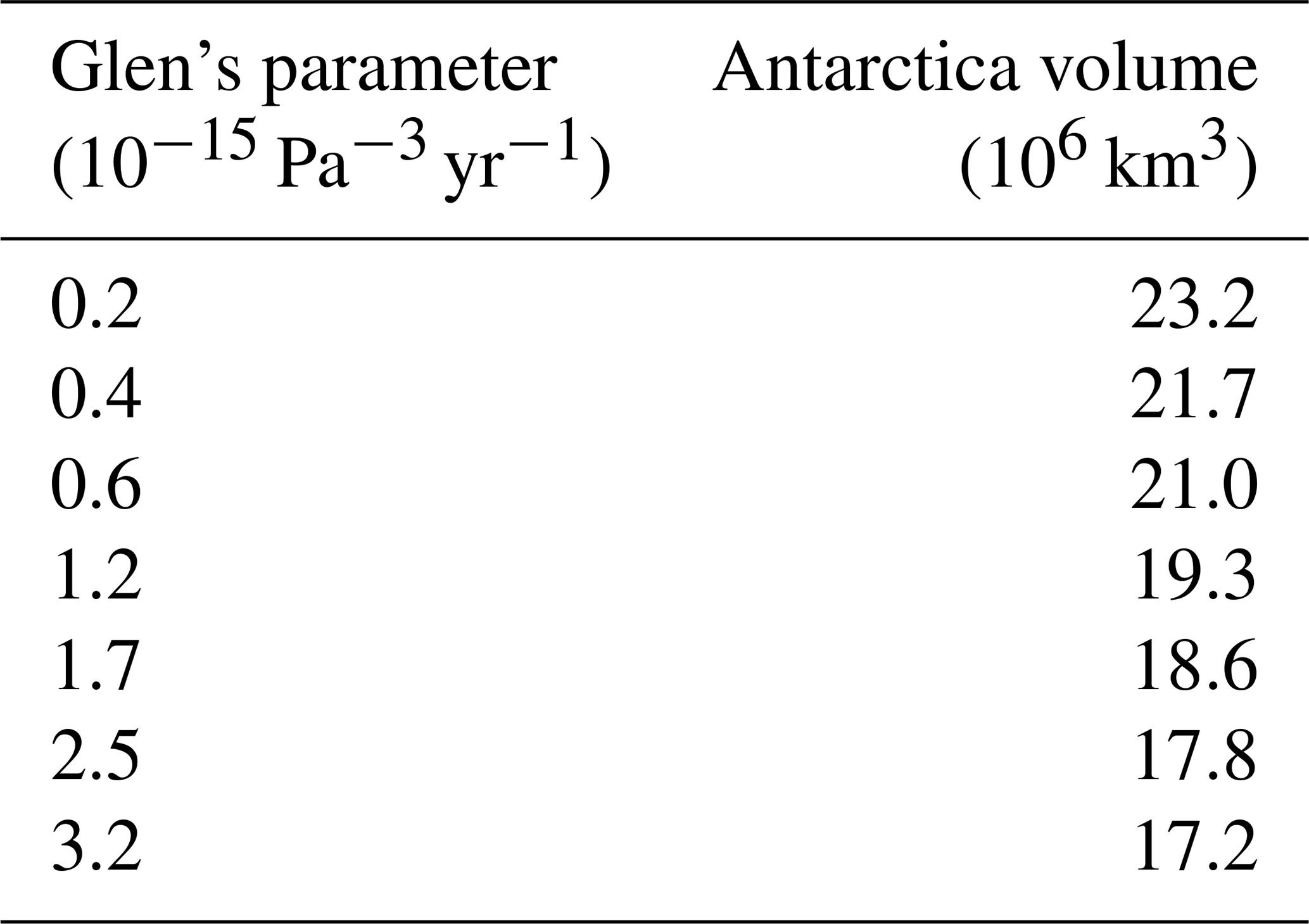
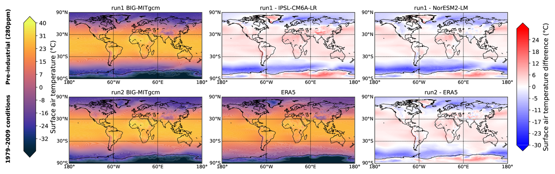
Figure A1 Surface air temperature averaged over 30 years for the pre-industrial conditions (first line) and the 1979–2009 conditions (second line). For the pre-industrial conditions, BIG-MITgcm run1 temperature distribution, IPSL-CM6A-LR and NorESM2-LM difference with respect to BIG-MITgcm run1. For the 1979–2009 conditions, BIG-MITgcm run2 and ERA5 temperature distribution, and ERA5 difference with respect to BIG-MITgcm run2.

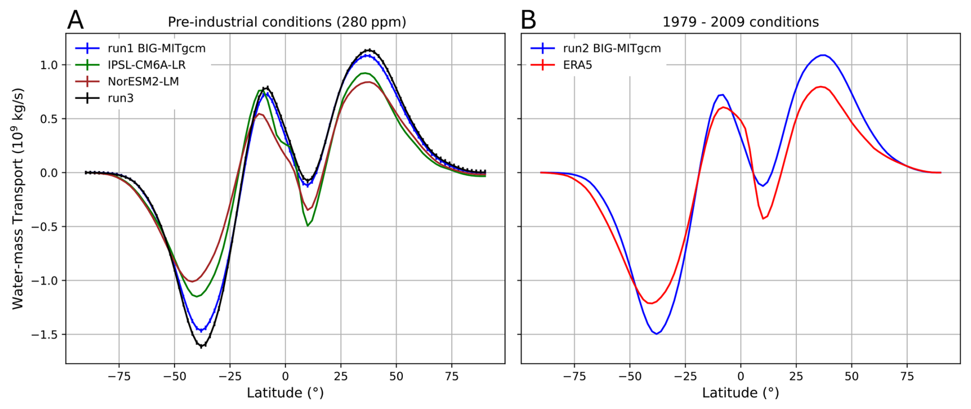
Figure A2 Zonal average of the northward water-mass transport in the atmosphere for the pre-industrial conditions (panel A) and the 1979–2009 conditions (panel B). Data are plotted using the Carissimo correction (Carissimo et al., 1985).

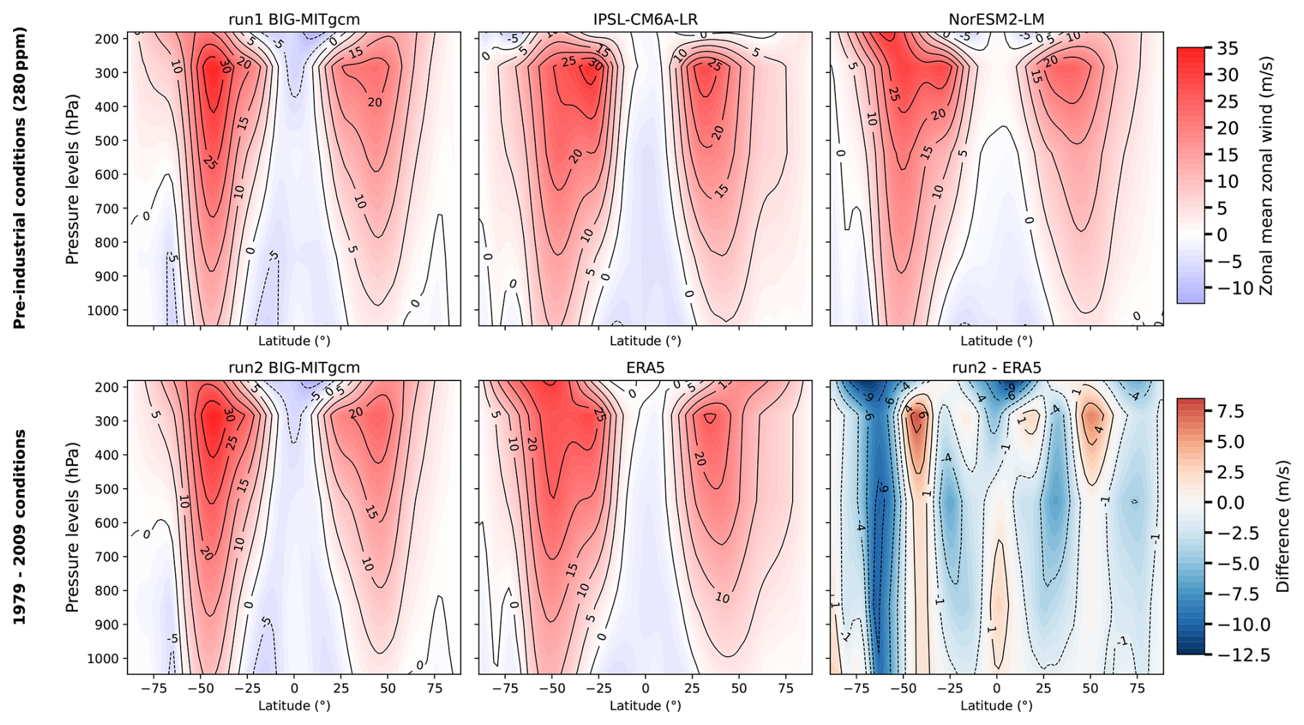
Figure A3 Zonal annual mean of zonal wind for the pre-industrial conditions (first line) and the 1979–2009 conditions (second line). For the pre-industrial conditions, BIG-MITgcm run1, IPSL-CM6A-LR and NorESM2-LM data are plotted in this respective order. For the 1979–2009 conditions, BIG-MITgcm and ERA5 distribution, and ERA5 difference with resepct to BIG-MITgcm run2.

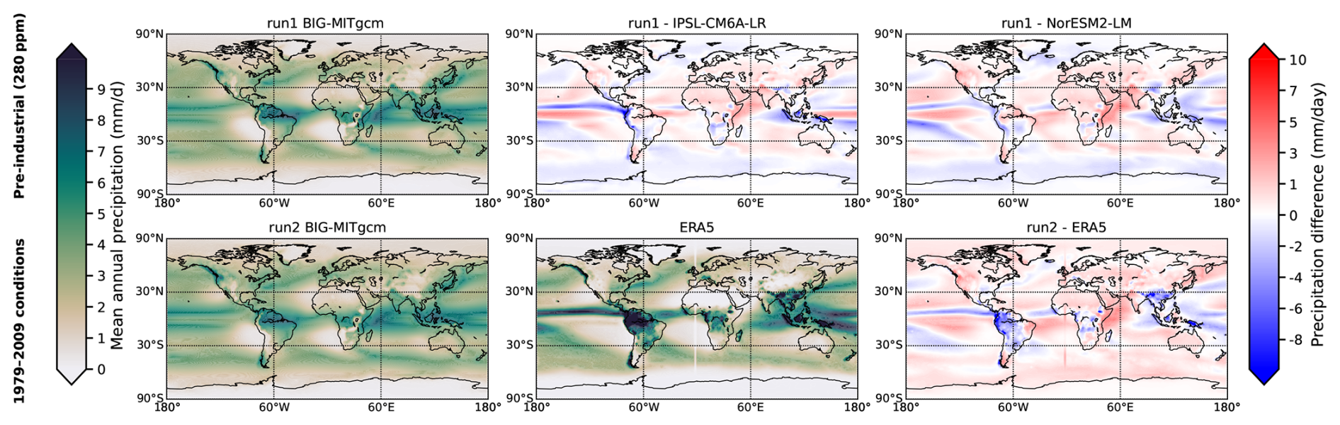
Figure A4 Precipitation averaged over 30 years for the pre-industrial conditions (first line) and the 1979–2009 conditions (second line). For the pre-industrial conditions, BIG-MITgcm run1 precipitation distribution, IPSL-CM6A-LR and NorESM2-LM difference with respect to BIG-MITgcm run1. For the 1979–2009 conditions, BIG-MITgcm run2 and ERA5 precipitation distribution, and ERA5 difference with respect to BIG-MITgcm run2.

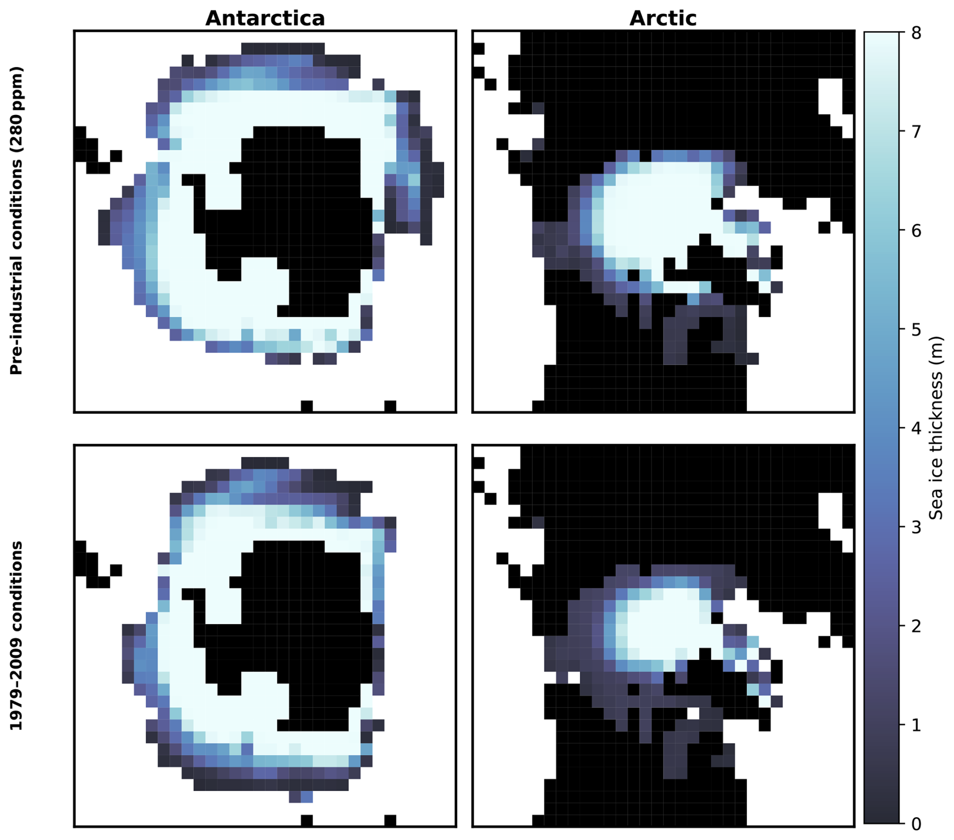
Figure A5 Annual mean sea ice thickness for BIG-MITgcm run1 (first line) and for BIG-MITgcm run2 (second line). The first column displays the Antarctica region and the second column the Arctic region. They are displayed on the cubed-sphere grid.

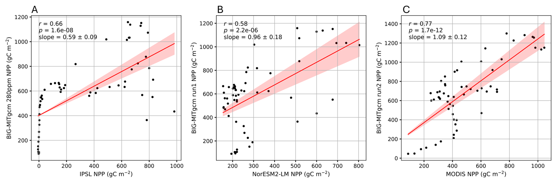
Figure A6 Linear regression (with corresponding r, p, and slope values) of NPP obtained with BIG-MITgcm run1 against IPSL-CM6A-LR (panel A), NorESM2-LM (panel B), and BIG-MITgcm run2 against the MODIS dataset (panel C).

Figure A7 Difference between BIG-MITgcm run1 and run3 for the surface air temperature and precipitation. Scales are the same as in the anomaly maps in Figs. A1 and A4.

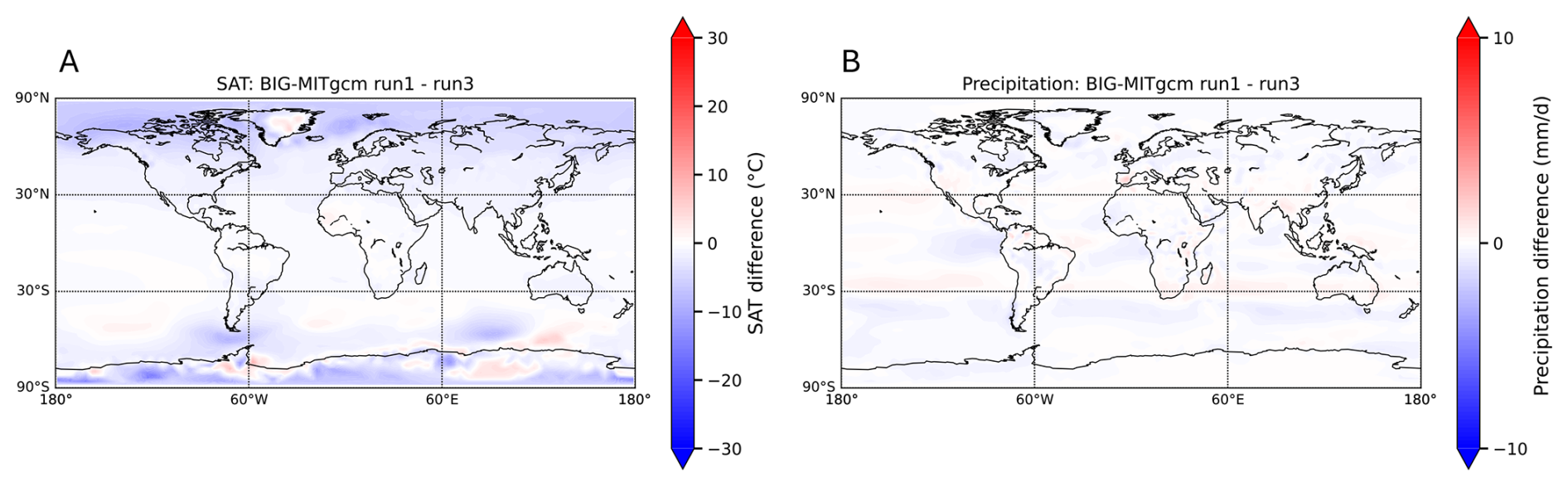
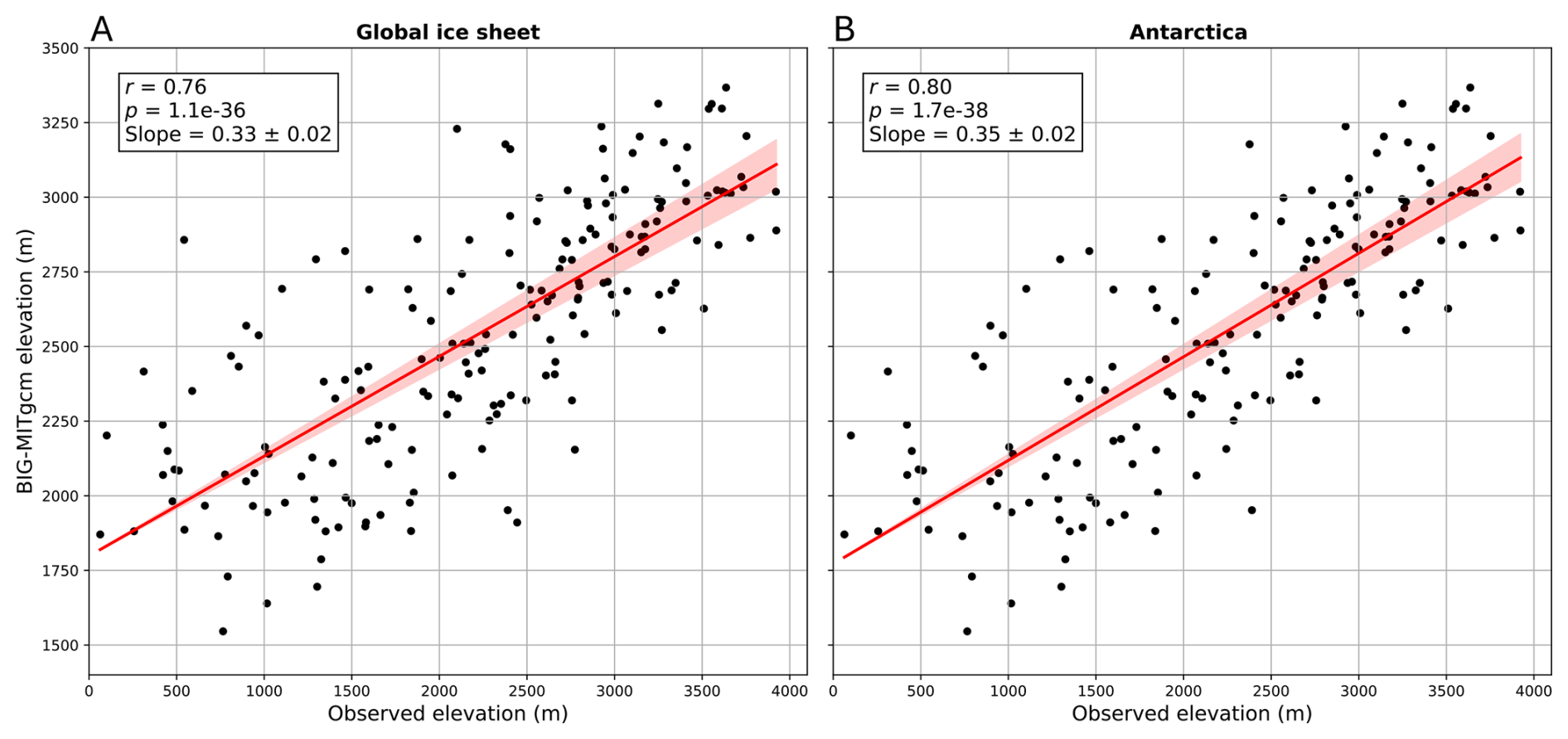
Figure A8 Correlations between the surface elevation of the ice sheets in BIG-MITgcm run1 and the BedMachine dataset for the global ice sheets (panel A) and Antarctica (panel B).

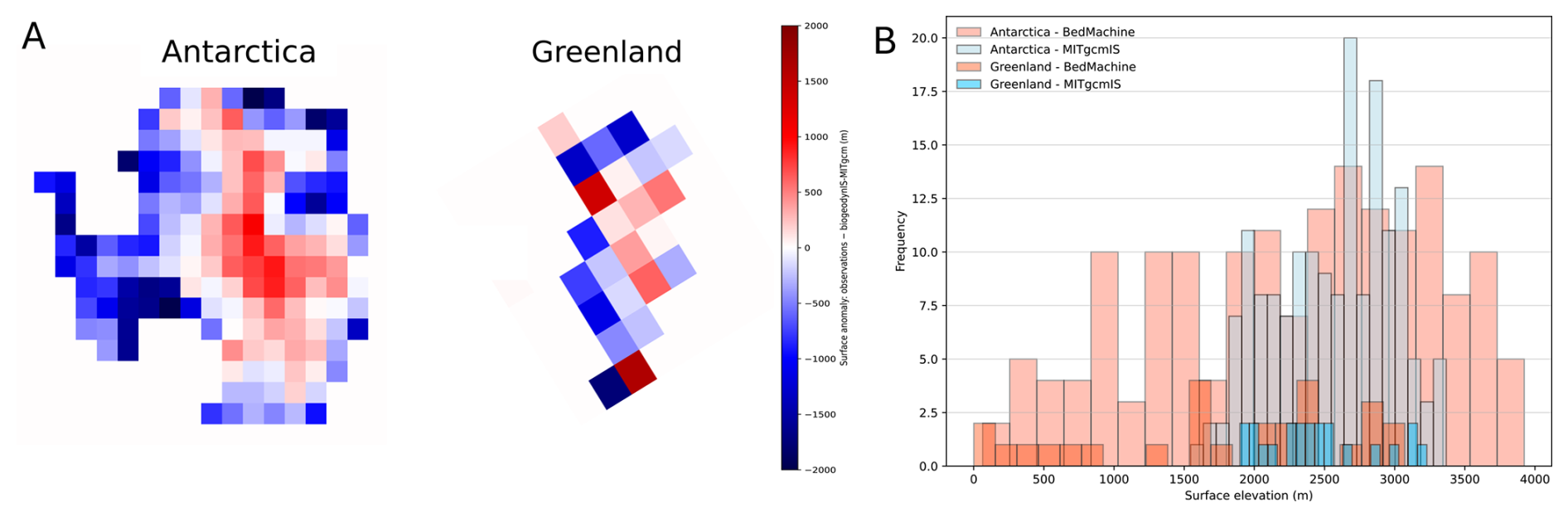
Figure A9 Anomaly maps of the surface elevation between the BedMachine dataset and BIG-MITgcm run1 for Antarctica and Greenland (panel A). Histograms of surface elevation where ice sheets form in BIG-MITgcm run1 (blue) and in the BedMachine dataset (orange) (panel B).