Two-tier MOM6 regional modelling suite of the East Australian Current system

We present a new ultra-high resolution $\mathrm{1}/\mathrm{30}$° (∼ 3 km) regional ocean model of the eastern Australian region and evaluate the performance of this model against two $\mathrm{1}/\mathrm{10}$° (∼ 10 km) models as well as a suite of satellite and in situ observations. We evaluate model biases in the context of (i) submesoscale-permitting (∼ 3 km) vs. mesoscale-permitting (∼ 10 km) horizontal resolution and (ii) differences between version 5 and version 6 of the Modular Ocean Model (MOM5 vs. MOM6) to assess the added value in each case and determine the suitability of our higher resolution model for scientific research. There are some consistent biases shared by the two regional MOM6 configurations, and also in the higher resolution configuration that are not seen in the lower resolution models. These biases are further investigated with two sets of sensitivity experiments to understand the effect of submesoscale eddy parameterization and imposed dynamic viscosity at a submesoscale-permitting resolution. The high-resolution simulation has much higher variance compared to the lower resolution simulations across all evaluation metrics, indicating that the greater spectrum of length scales also manifests in more variability in the temporal domain. The two MOM6 regional configurations of differing resolution appear to be more aligned than the regional (MOM6) and global (MOM5) $\mathrm{1}/\mathrm{10}$° configurations in most results, reflecting the substantial changes made to the MOM between version 5 and version 6. Importantly, we also show that higher resolution is not a panacea: in regions where key dynamics are quasi-linear and well-captured captured by coarser grids (e.g., the EAC jet), further refinement may offer limited benefit – and actually degrade the performance if parameterizations are not appropriately tuned.

1 Introduction

The East Australian Current (EAC) is a western boundary current (WBC) that begins as a coherent poleward jet along the shelf break off north-eastern Australia (from 15° S) before separating from the shelf typically around 32° S and forming large mesoscale eddies that tend eastward towards New Zealand, or poleward along the south-east Australian margin (Godfrey et al., 1980). The EAC has a leading order influence on the physical, biological and nutrient conditions in the shelf waters of eastern Australia (Roughan et al., 2022; Suthers et al., 2011; Chapman et al., 2024). Although the upstream jet component of the EAC has not changed significantly over the past half century (Sloyan and O'Kane, 2015; Sloyan et al., 2024), this steadiness does not extend poleward into the separation region and downstream eddy field which have changed markedly. The separation of the EAC is tending to occur at its poleward limit more often (Cetina-Heredia et al., 2014), whilst the energetics associated with separation and the episodic eddy shedding have intensified (Li and Roughan, 2023; Malan et al., 2021). Downstream of this region, along the most densely populated part of the Australian coastline, a strengthening eddy field has driven an ocean warming rate well above the global average for the past century (Ridgway, 2007; Li et al., 2022a). Our understanding of the processes connecting the offshore warming to the nearshore regions of south-east Australia is still limited, and urgent attention targeting this rapidly changing system is needed to inform decision making on seasonal to decadal time scales.

Much of what we currently understand about ocean-shelf connectivity in the EAC system has been derived from a long-standing configuration of the Regional Ocean Modelling System (ROMS; Kerry et al., 2016). Here, we describe the development of an alternative regional model based on the Geophysical Fluid Dynamics Laboratory's (GFDL's) Modular Ocean Model, version 6 (MOM6) at a nominal 3 km resolution. Following the recent approach taken in MOM6 regional modelling of the north-west Atlantic (Ross et al., 2023) and the north-east Pacific (Drenkard et al., 2024), we have opted for a “coastwide” model domain that encapsulates the entire EAC system and the eastern boundary of Australia. The previous ROMS modelling of this region has focused on a spatial subset centred around the EAC separation point that neglects the upper and lower limits of the EAC and adjacent coastline. Chapman et al. (2025) identified an upstream control through eddy-jet interactions that can substantially modulate the conditions in the eddy-dominated EAC extension region, highlighting the importance of resolving the EAC's origins to the north. The southern half of the EAC extension is where physical and ecological changes are most accelerated and many species range distributions are already contracting significantly (Ling et al., 2009). While our MOM6 regional model is not expected to outperform ROMS in all aspects of the overlapping domains, we believe the challenge of understanding the EAC's influence on eastern Australia, in the context of a rapidly shifting large-scale mean state warrants exploration through complementary modelling frameworks to build a more robust understanding of ocean-shelf connectivity. Furthermore the fact that ROMS is a terrain-following vertical coordinate model while MOM6 adopts the novel Arbitrary Lagrangian Eulerian (ALE) coordinate system of Griffies et al. (2020) is likely to reveal some different insights into the dynamics, particularly along the steep topographic gradient of the continental slope (Haney, 1991; Haidvogel et al., 2008).

We assess the improvements gained in modelling the EAC system at higher resolution – specifically focusing on the four key dynamical regimes of this system: the coherent EAC jet; the highly variable EAC separation point; the energetic, eddy-dominated EAC extension region and the narrow continental shelf. We hypothesize that increasing horizontal resolution will provide the greatest benefits (in terms of reducing model bias) in the turbulent eddy field of the EAC extension, whereas upstream, the quasi-linear dynamics of the EAC jet are already well resolved at 10 km, likely leading to diminishing returns for further resolution increases in the jet region. The separation dynamics of the EAC are driven by the growth of barotropic and baroclinic instabilities, while typically barotropic instabilities dominate (Mata et al., 2006; Bowen et al., 2005; Bull et al., 2017; Li et al., 2021). Increasing the resolution should allow a better representation of both instability pathways, likely improving the modelled separation and eddy shedding dynamics. The growth of instabilities during EAC eddy shedding events in the separation latitudes will be sensitive to the choice of horizontal viscosity. We will explore how the 3 km model responds to changes in this parameter choice, as well as changes in the length scale associated with the mixed layer eddy (MLE) parameterization (Fox-Kemper et al., 2011). The results from this study will provide the ocean modelling community with a new test case for the MOM6 regional modelling framework, advance our understanding of parameter sensitivity in western boundary currents, and establish a foundation for future investigations into the EAC's role in shaping nearshore physical and biogeochemical variability.

The remainder of the paper is structured as follows: Sect. 2 details the approach taken in configuring a two-tier nested regional MOM6 configuration, along with the rationale behind a set of two sensitivity tests to assess parameter choices when moving to submesoscale-permitting resolutions. Section 3 presents the results of the model evaluation and sensitivity experiments, while Sect. 4 discusses the conclusions and provides recommendations for high-resolution modelling and the tuning of subgrid-scale parameters.

2 Methods

Here, we introduce the two-tier nested model suite for the EAC region which we developed following a similar approach to Herzfeld et al. (2011), and then outline the set of parameter sensitivity experiments we carried out to further explore the biases in the nested configuration.

2.1 Two-tier nested suite

The hierarchical design of the nested modelling suite is shown in Fig. 1, and consists of a “parent” global model, enclosing a large regional model, further enclosing a small regional model that spans the entire EAC system. The global model used is the Australian Community Climate and Earth System Simulator – Ocean Model v2 1/10th degree horizontal resolution configuration (hereafter referred to as OM2-01) (Kiss et al., 2020), which uses a Mercator grid, such that the horizontal grid spacing scales with cosine of latitude. The large regional model named “STHPAC10K” (referring to the partial basin-scale “South-west Pacific” that it encompasses) takes the horizontal and vertical grids, topography and open boundary forcing directly from OM2-01. The higher resolution model of the East Australian current region, named “EAC03K” has horizontal resolution three times higher in both zonal and meridional directions (i.e., nine grid cells for every one in STHPAC10K), 25 more vertical levels, an updated topography dataset (GEBCO2022 vs. GEBCO2014; Kapoor, 1981), and takes open boundary forcing from STHPAC10K. Both regional models adopt the Mercator grid projection of the OM2-01 global model. We have chosen to use the metric of distance (e.g., “EAC03K”, “STHPAC10K”), rather than degrees (e.g., “EAC-003”, “STHPAC-01”) as the naming conventions for our regional models. Throughout this paper, when discussing differences between the coarser models (OM2-01, STHPAC10K) and the high resolution model (EAC03K), we will use the terms “10 km models” and “3 km model” respectively. Our regional simulations have been configured using the regional-mom6 software package described by Barnes et al. (2024).

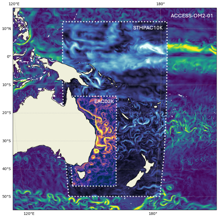
Figure 1 Map demonstrating the two-tier nesting approach taken for our MOM6 regional modelling endeavour. The outer dashed box delineates our 10th degree (10 km) large regional model named STHPAC10K. The inner dashed box encapsulates our 30th degree (3 km) small regional model named EAC03K. The shading shows a snapshot of surface speed across the three models to demonstrate the effectiveness of the open boundary conditions in transmitting signals into and out of the model domains (noting that our models are only one-way nested).

Stewart et al. (2017)Arakawa and Lamb (1977)Kapoor (1981)Griffies and Hallberg (2000)Adcroft et al. (2019)Flather (1976)Orlanski (1976)

Table 1 Summary of model configuration choices for the double-nested experiments (adapted from Ross et al., 2023).

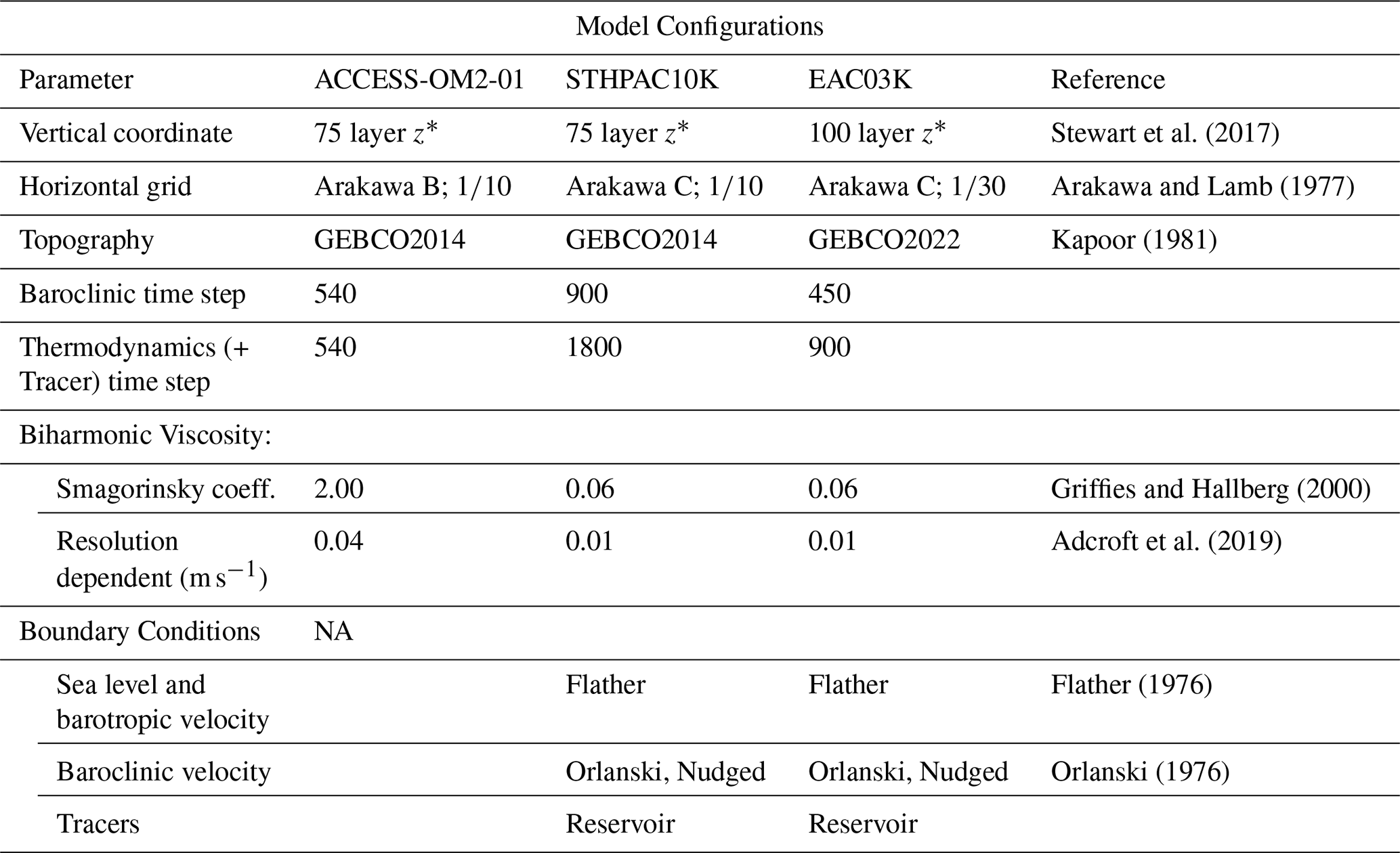
Table 1 summarizes the key parameters used in the parent, large regional, and small regional models. For the MOM6 regional models in our initial nesting experiment, we adopt most parameter choices taken in Adcroft et al. (2019). MOM6 employs a generalized vertical coordinate framework based on the Arbitrary Lagrangian-Eulerian (ALE) method, in which the ocean state is first advanced using a vertical Lagrangian timestep and is then periodically regridded and remapped onto a prescribed target grid (Adcroft et al., 2019; Griffies et al., 2020). The z^∗ coordinate system employed by Kiss et al. (2020) for their OM2-01 configuration is the chosen target grid in our regional models, for consistency with the parent model, and for its improved representation of the steep bathymetric gradients when vertical resolution permits. For all models, the vertical resolution is finest in the upper ocean, and coarsens with depth. The number of layers is guided by Stewart et al. (2017), considering the baroclinic modes resolved by the horizontal grid, and ensuring the vertical grid is capable of resolving the vertical structure of those horizontal modes. Stewart et al. (2017) note that 50 levels is sufficient for resolving the first baroclinic mode, with an additional 25 levels required for each further mode. In the next section we will show that 3 km horizontal resolution over the EAC domain can approximately resolve up to the third baroclinic deformation radius – hence justifying the use of 100 vertical levels for this configuration.

The different horizontal grid schemes between the MOM5 and MOM6 is a major source of discrepancy between the two 10 km models compared in this study. The parent global model employs an Arakawa B grid, while the MOM6 based regional models employ Arakawa C grids (Arakawa and Lamb, 1977). In B grids, the velocity points are co-located in the north-west corner of the grid cell, whereas in C grids, the u and v points are offset to the eastern and northern edges of the grid cell respectively. At coarse resolutions, this staggering of the velocity components in C grids can introduce numerical errors, particularly in the representation of large-scale balanced flows (Griffies et al., 2000). For this reason, B grids have historically been preferred in global models with coarse resolution (Griffies et al., 2000). However, C grids offer significant advantages at higher resolutions – especially in their ability to more accurately represent energy cascades and the nonlinear dynamics of baroclinic eddies. Since capturing these eddy processes is a key goal of the EAC03K configuration, the use of MOM6 and the C grid is well aligned with the scientific objectives of our study.

2.1.1 Horizontal resolution

The choice of horizontal resolution for EAC03K was based on the length scales that we are interested in resolving within the EAC system. To understand the range of dynamics that we expect to resolve, one must consider the horizontal grid spacing with respect to the internal deformation radii of the region (Hallberg, 2013). This relationship is approximated by

$$\begin{array}{}\text{(1)}& R_{\mathrm{H}}={\displaystyle \frac{L_{\mathrm{d},\mathrm{1}}}{\mathrm{\Delta }}}=\sqrt{{\displaystyle \frac{\frac{c_{\mathrm{g}}^{\mathrm{2}}}{f^{\mathrm{2}}+\mathrm{2}\mathit{\beta }{c}_{\mathrm{g}}}}{\frac{\mathrm{\Delta }{x}^{\mathrm{2}}+\mathrm{\Delta }{y}^{\mathrm{2}}}{\mathrm{2}}}}}\end{array}$$

where L_d,1 is deformation radius of the first baroclinic mode, c_g is the associated gravity wave speed, f is the Coriolis parameter, and $\mathit{\beta }=\partial f/\partial y$ is its meridional gradient. The approximate grid size Δ is taken as the average of the grid length along the two horizontal axes, Δx and Δy.

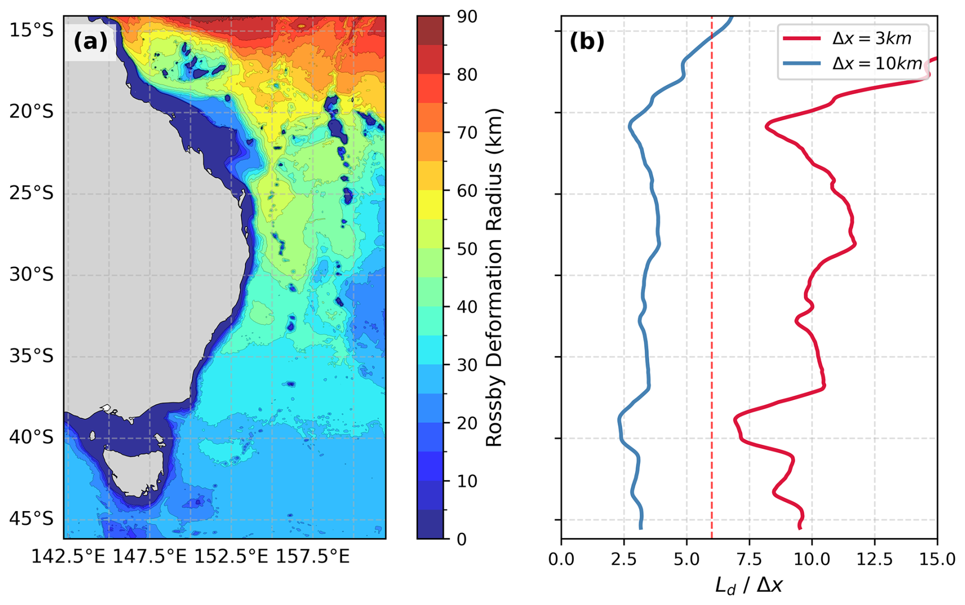
Figure 2 (a) First baroclinic mode Rossby radius of deformation (L_d,1) for the EAC domain. (b) Ratio of zonally averaged deformation radius to the model grid spacing for EAC03K (red) and 10 km models (STHPAC10K, OM2-01) (blue). Vertical red dashed line in panel (b) shows the ratio value of 6 identifying where the first three baroclinic modes are approximately resolved.

We show the spatial distribution of the first baroclinic deformation radius in Fig. 2a, whereby typical open ocean values exceed 90 km towards the equator, and contract poleward to around 20 km in the mid-latitudes – primarily controlled by the increased effect of the Coriolis parameter towards the poles. The ratio of this length scale to the respective grid spacings of the two resolutions is shown in Fig. 2b, where the difference between the two models is very clear. The horizontal resolution of the 10 km models (STHPAC10K and OM2-01) yields a $L_{\mathrm{d},\mathrm{1}}/\mathrm{\Delta }x$ ratio of approximately 2.5 across most latitudes, while the EAC03K model exceeds a ratio of 6 throughout (Fig. 2b). According to Hallberg (2013), a ratio of at least 2 is sufficient to omit the Gent-McWilliams (GM) mesoscale eddy parameterization (Gent et al., 1995), as the grid is fine enough to partially resolve large-scale eddy effects. This justifies the exclusion of GM in our 10 km configuration. However, resolving the full dynamical influence of mesoscale eddies on the general circulation – particularly their energy cascades and interactions with topography – requires finer resolution. Hallberg (2013) recommend a ratio of 6 for this purpose, and EAC03K meets this criterion across the entire domain (Fig. 2b). At this resolution, the model can begin to capture higher-order baroclinic modes, likely resolving up to the third baroclinic mode in the open ocean, and on the order of the first baroclinic mode over the shelf (Hallberg, 2013). Combined with the increased vertical resolution (Stewart et al., 2017), this horizontal resolution leads to a well-resolved mesoscale regime for EAC03K throughout the domain, whereby scale interactions are free to self-regulate without diffusive parameterizations suppressing the variability. Hallberg and Gnanadesikan (2006) demonstrate that explicitly resolving mesoscale eddies leads to increased transport within these coherent features. We anticipate this will lead to an improved representation of the EAC extension eddy field, and subsequent improvement in temperature variability both inshore and offshore of the continental shelf along south-eastern Australia (Malan et al., 2020).

2.1.2 Forcing

To ensure consistency across model configurations, the two regional models use the same atmospheric forcing as the global model (OM2-01): version 1.5 of the Japanese Reanalysis for Driving Oceans (JRA55-do v1.5; Tsujino et al., 2018). The historical simulations span 1990–2020, using interannual forcing (IAF) to capture the large-scale climate variability and long-term change over three decades. Surface momentum fluxes are computed online within MOM6 from these prescribed atmospheric fields using a relative-wind formulation, such that the applied wind stress depends on the difference between the 10 m wind and the model surface ocean velocity. In an ocean-only configuration, this relative-wind formulation is expected to reduce the net wind work on the ocean circulation, and can damp mesoscale eddy variability relative to simulations forced with direct winds (Renault et al., 2016).

Tidal forcing and river inputs are omitted in the regional configurations, as our focus is on the deep ocean circulation's influence on shelf conditions, and river runoff in the Australian region is relatively low. We are primarily interested in the ocean dynamics governing connectivity across the shelf break and not necessarily the localised processes driving variability within the inner shelf region (< 200 m). Previous studies of different sections of the shelf along eastern Australia have found very little influence from tidal and river forcing on shelf conditions away from the estuaries and inner shelf (Oliver et al., 2016; Li et al., 2022b).

2.2 Parameter Sensitivity Experiments

Two sets of parameter sensitivity experiments were performed using EAC03K in order to improve our understanding of model sensitivity to the mixed-layer eddy restratification and dynamic viscosity at submesoscale-permitting grid resolutions. Due to computational constraints, these experiments had a shorter duration of 10 years. However global diagnostics indicate the simulations reached a relatively steady state after about 2 years (not shown). Furthermore, two additional tests were conducted to address (i) senstivity to boundary conditions (BCs): does the interior solution change if we force the EAC03K configuration with OM2-01 rather than STHPAC10K? and (ii) sensitivity to initial conditions (ICs): does initialising the EAC03K configuration from a 10 year long repeat year spin-up improve the solution?

2.2.1 Mixed-Layer Eddy Parameterization

The first sub-grid parameterisation sensitivity experiment concerns the Mixed-Layer Eddy (MLE) scheme. In MOM6, this scheme acts to restratify the mixed layer in the presence of sharp horizontal buoyancy gradients (Fox-Kemper et al., 2011), and has been shown to influence mixed-layer structure and sea surface temperature, particularly in coarser-resolution models where mixed-layer eddies are unresolved (Adcroft et al., 2019; Ross et al., 2023). Here, however, our aim is not to evaluate MLE in that established coarse-resolution setting, but to test whether it remains influential in the 3 km EAC03K configuration, where submesoscale variability is partially resolved and some mixed-layer restratification processes may begin to be represented explicitly.

The sensitivity of this scheme is controlled by a single dimensional parameter, the frontal length scale, which is on the order of the mixed layer deformation radius, $NH/f$ (where N is the buoyancy frequency and H is the mixed layer depth) and acts as a lower bound upon which a mixed-layer overturning streamfunction is scaled via

$$\begin{array}{}\text{(2)}& \mathit{\Psi }\propto {\displaystyle \frac{\mathrm{\Delta }s}{L_{\mathrm{f}}}}\end{array}$$

where Δs is the model horizontal grid scale, and the frontal length scale is chosen as

$$\begin{array}{}\text{(3)}& L_{\mathrm{f}}=max\left(NH/\left|f\right|,L_{\mathrm{f},min}\right).\end{array}$$

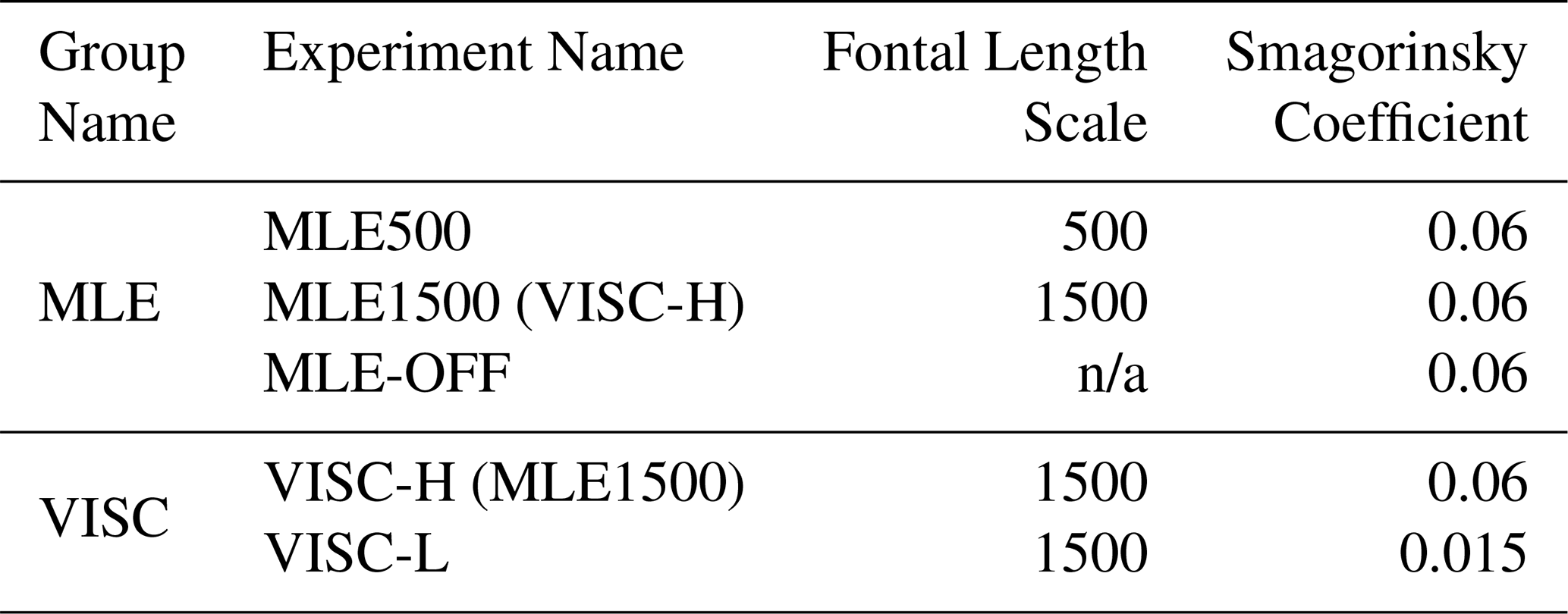
The base value for the nested simulations was $L_{\mathrm{f},min}=\mathrm{500}$ m (Adcroft et al., 2019), whilst we run two additional sensitivity experiments, with $L_{\mathrm{f},min}=\mathrm{1500}$ m and with the parameterization turned off entirely (Table 2). A larger minimum length reduces the influence of the parameterization, and the mixed layer will not restratify as much in response to strong horizontal gradients. This is expected to have an impact on the SST long-term statistics. It is uncertain whether the scheme is needed at higher resolutions, hence turning it off will reveal insights into the model's ability to resolve processes associated with large mesoscale eddy strain.

Table 2 Sensitivity experiments performed to assess two important parameterizations influencing the model fidelity.

In order to investigate the influence of the Fox-Kemper MLE parameterization (Fox-Kemper et al., 2011), we additionally assessed biases in the mixed layer depth (MLD) against the Global Ocean Reanalysis and Simulations (GLORYS12V1; (Lellouche et al., 2021) reanalysis product. This reanalysis was chosen due to its high resolution and duration spanning the majority of our model duration, with a start date of 1993.

2.2.2 Dynamic Viscosity

The second sensitivity test assess the model response to the dynamic viscosity parameterization, referred to throughout as VISC. Numerical modelling of WBC regimes has historically revealed a large sensitivity to the horizontal viscosity parameterization used in the model. In the Euler momentum equations of geophysical fluid dynamics, viscosity acts to dampen the linear terms, and suppress growth of the nonlinear terms whilst the precise nature of the effect depends on whether a Laplacian or biharmonic velocity scaling is employed (Griffies and Hallberg, 2000). The biharmonic approach has proven to be most effective at suppressing grid-scale noise whilst preserving energy at large scales and is used with the Smagorinsky dynamic viscosity scheme for all configurations in this paper (Griffies and Hallberg, 2000; Smagorinsky, 1963).

Ross et al. (2023) note a strong sensitivity of the Gulf Stream separation in their MOM6 based regional model to the biharmonic viscosity whereby higher viscosities lead to a more poleward separation of the WBC, whilst lower viscosities lead to an earlier, equatorward separation. They note this viscosity response to be typical and consistent with earlier studies (e.g., Bryan et al., 2007; Chassignet and Garraffo, 2001). However Tilburg et al. (2001), albeit using a simplified 1.5 layer reduced-gravity linear model of the EAC system, found the opposite effect – a weaker viscosity led to a more poleward separation, whilst a stronger viscosity led to an equatorward separation.

These two contradicting cases highlight the important and competing processes driving WBC separation. In the nonlinear case of Ross et al. (2023), instabilities grow through baroclinic and barotropic processes, generating eddies that disrupt the coherent WBC and drive separation. Since viscosity damps these instabilities, a higher viscosity suppresses the turbulence and delays separation, whereas a lower viscosity allows faster eddy growth and earlier separation. In the linear case, however, separation is dictated by the large-scale wind stress curl and planetary vorticity balance, rather than instability-driven processes. In this system, viscosity dissipates momentum from the WBC, reducing its inertial resistance to the wind-driven gyre circulation. As a result, a higher viscosity weakens the WBC, making it more susceptible to turning eastward at a lower latitude, whereas a lower viscosity allows a stronger WBC that can persist farther poleward before separating.

We adopt the dynamic viscosity scheme chosen by Ross et al. (2023) whereby the imposed horizontal viscosity is the maximum of two quantities. The first is a predetermined velocity scale multiplied by the cube of the grid spacing $u_{\mathrm{4}}{\mathrm{\Delta }}_x^{\mathrm{3}}$, while the second is the biharmonic Smagorinsky viscosity – a dynamic flow-dependent quantity. The coefficients of the Smagorinsky viscosity were set to 0.06 in the double-nested and MLE experiments, which is the recommended upper bound for the MOM6 model (Adcroft et al., 2019). To test an alternate case, we take the MLE-1500 experiment from the MLE tests, and refer to this as the high viscosity run (VISC-H), while we run one additional experiment – VISC-L – with a Smagorinsky coefficient set at the lower bound of the MOM6 recommended range, 0.015 as also used in the Ross et al. (2023) NWA12 model (Table 2).

2.3 Model evaluation

We evaluate the model configurations against observational and reanalysis products as specified below, and compare their behaviour across a set of region-specific diagnostics. We note that the three configurations considered here (OM2-01, STHPAC10K, and EAC03K) differ in more than one aspect, including model framework, domain configuration, and horizontal and vertical resolution. Accordingly, the model evaluation is not intended as a controlled, single-factor attribution study of individual model settings. Rather, its purpose is to provide a contextual evaluation across two broad axes of model development that are central to this study: (i) the transition from MOM5 to MOM6, and (ii) the refinement from 10 to 3 km resolution within the nested MOM6 framework. Observations and reanalysis products are used as an external reference to assess whether the net cumulative changes lead to improved representation of the EAC system. Controlled sensitivity experiments designed to isolate the impact of specific parameter choices are presented separately in Sect. 3.2.

2.3.1 Region-wide evaluation metrics

Daily sea surface temperature (SST) fields from all models are compared with the National Oceanic and Atmospheric Administration SST product, developed using optimum interpolation (OISST; Reynolds et al., 2007). The OISST product combines satellite and in situ observations and is representative of the top 0.5 m of the ocean. Daily sea surface height fields (SSH) fields are evaluated against the Archiving, Validation, and Interpretation of Satellite Oceanographic data (AVISO) altimetry-derived SSH product.

All region-wide metrics are evaluated over the EAC domain (Fig. 1, EAC03K box) and all model grids are bilinearly interpolated onto the observational products' horizontal grid. The root mean square error (RMSE) at each coarsened model grid point is calculated and the spatial average of this metric is computed in order to assess overall differences between datasets.

Marine heatwave (MHW) analysis has also been performed on the surface SST fields of all datasets, following the approach of Hobday et al. (2016). The SST fields are first regridded to the coarser OISST (∼ 25 km) grid using bilinear interpolation, and then we computed the daily-varying climatology and the 90th percentile threshold temperature at all grid points in the EAC domain. We then use the 90th percentile temperature as a lower bound and identify all anomalies exceeding this. If the temperature persists above this threshold for greater than 5 days, we record this as a MHW event and various metrics are stored for the event such as the anomaly above the 90th percentile temperature, and the duration.

2.3.2 Region-specific metrics

The EAC jet flows coherently along the shelf break of southern Queensland and northern New South Wales between latitudes 14–32° S. In 2012, a mooring array was established at 27.5° S to gain insight into the subsurface structure and variability of the jet upstream of the separation point (Sloyan et al., 2024). This mooring array was in operation until 2022, allowing almost a decade of high spatial and temporal resolution in situ measurements of the jet. In this jet regime, we are interested in whether the regional models can represent the seasonal cycle of volume transport identified in observations. We compute poleward transports within the longitudinal range of the mooring array, and calculate the climatology over the simulation period. We do not take into account interannual differences here, and compare the climatologies calculated from 30 year model simulations with that from the ∼ 10 year observational period.

In order to identify where the EAC separates from the coast in each model (and observations), we established two distinct definitions that describe this process – the “separation latitude”, and the subsequent “retroflection latitude”. Adapting the approach of Cetina-Heredia et al. (2015), we choose a SSH contour that best represents the path of the EAC jet at 28° S and follow this poleward to the “separation latitude”, defined as the variable point where this contour exceeds a zonal distance of 80 km from the 2000 m isobath (Fig. 7a, b). Following the contour further south, we define the retroflection point where the tangent of this contour veers due east (i.e., tangent vector transitions from the south-east quadrant to the north-east quadrant (Fig. 7a, b). We make the distinction between the two points since the dynamics controlling the pair of latitudes are likely semi-independent, however no distinction has been made previously between the two separate processes. Adopting this more nuanced definition of the WBC separation latitudes has revealed new insights into the controlling dynamics of both the separation and retroflection latitudes.

Additional improvements on the approach taken by Cetina-Heredia et al. (2015) were necessary to account for cyclonic frontal eddies developing inshore of the EAC jet (Schaeffer et al., 2017), leading to the temporary detachment and re-attachment of the jet upstream of the main separation latitude. Cetina-Heredia et al. (2015) choose the SSH contour that aligns with the maximum poleward velocity of the upstream EAC jet, which in our 3 km model, led to approximately 20 % of the timesteps failing to identify an appropriate pair of separation/retroflection latitudes. An improvement was achieved when smoothing the nominated SSH contour using a simple coarsened linear interpolation which removed the effect of frontal eddies that pushed the contour offshore, only for it to reattach ∼ 50 km downstream. However, further improvement was achieved by deciding to choose the SSH contour based on an iterative process, similar to that of (Chapman et al., 2025), whereby we first detect the longest positively-sloped segment of a zonal SSH transect at 28° S and assume (via geostrophy) this represents the poleward EAC jet at this latitude. Then, starting from the western extent of the segment, we follow the SSH contour originating at that point to see whether it is a good representation of the EAC jet. This decision is automated and primarily based on the length of the contour and a sensible result for the detected points. This is repeated at each timestep until a suitable SSH contour is found, which has resulted in a vastly improved failure rate less than three percent. The failed timesteps show SSH contour maps with no sign of an EAC jet present, highlighting the variable nature of the EAC system as a whole.

The most variable component of the EAC system and potentially the most important for our interests in the south-east Australian region is the eddy field (aka “Eddy Avenue”; Everett et al., 2012) poleward of the EAC separation point. There is a direct relationship between the growth of instabilities in the EAC separation region and eddy characteristics in the EAC extension (Li et al., 2021). As such, if there are biases in the separation dynamics, these are likely to cascade into the EAC extension eddy characteristics in our model. To get a synthesis of the eddy variability in this region, we perform an eddy tracking using the python package py-Eddy-Tracker (Delepoulle et al., 2022) which can efficiently track the size and polarity of eddies over the 30 year analysis period from the SSH fields. We then calculate the mean amplitude of eddies within coarsened grids (25 × 25 km) which provides a metric to understand the amount of eddy kinetic energy (EKE) present spatially in the model domain.

We anticipate a higher resolution model to have improved connectivity across the shelf break, due to important scales of variability being better represented at 3 km resolution. Here we are interested in assessing how well the different models produce the SST warming rates along the shelf of eastern Australia. We take polygons of all the bioregions that are designed to capture quasi-homogeneous oceanographic and ecological conditions in the nearshore domain (O'Hara et al., 2016). Sea surface temperatures within each bioregion are then spatially averaged to obtain a daily SST time-series for each bioregion and then the linear trend is calculated. We further group the time-series by season and re-calculate the SST trends to understand whether or not the trends are ubiquitous across seasons. In order to further validate the model results, we use an additional observational dataset produced specifically for the Australian region, namely Integrated Marine Observing System SST (IMOS-SST) satellite product (Griffin et al., 2017). The IMOS-SST product has a resolution of 0.02° and has proven to be more reliable than OISST in representing temperature trends and variability closer to the coast (Beggs et al., 2018).

3 Results

3.1 Nested Experiments

3.1.1 Surface Fields

The mean SST biases in the global model are relatively weak and spatially patchy, whereas STHPAC10K exhibits minimal bias and closely aligns with observations (Fig. 3b, c). In contrast, EAC03K shows a pronounced cold bias in the EAC extension, accompanied by a warm bias in the mid-latitude eastern sector of the domain (Fig. 3a). This pattern may indicate a weaker poleward transport of the EAC, with an associated redistribution of heat toward the eastern boundary. In terms of the SST trends, all models capture the broad pattern of faster warming in the EAC extension (not shown), however EAC03K shows a much more concentrated, coastal-bound warm pool off south-east Australia (Fig. 3d).

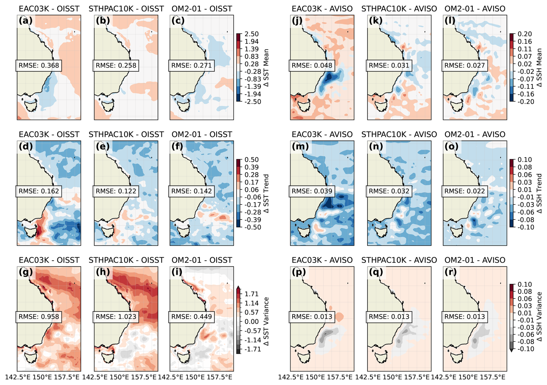
Figure 3 Surface biases of the three models relative to observations for SST (left) and SSH (right). The top row represents Mean bias, middle row represents Trend bias, and the bottom row shows Variance bias for both prognostic variables.

When comparing the SST variance from a model, which represents day-to-day variability, to OISST, which represents a smoothed 5 d window of variability, we expect to find a systematic positive bias for all modelled SST variance due to the reduced spatial and temporal interpolation in the models (Reynolds et al., 2007). This expectation holds true for our 3 km model, EAC03K, whereby there is a tendency for larger variance (positive bias) across the entire domain (Fig. 3g). Importantly, in the EAC extension region, both 10 km models produce less variability than the already dampened OISST, suggesting that these models may under-represent the intensity or frequency of eddy-driven temperature fluctuations off south-east Australia (Fig. 3h, i). Both regional models exhibit an expansive north-west to south-east oriented band of high variance across the northern half of the domain, having the appearance of an imprinted south Pacific convergence zone (SPCZ) that is not present in observations or the global model (Fig. 3g, h). Given all models use the same version of JRA55 atmospheric interannual forcing, this is likely associated with the updated surface flux numerics in MOM6. However it appears to be independent of other biases and hence is not further explored in this paper.

At 10 km resolution, MOM6 appears to slightly improve on MOM5 in representing the mean SST pattern compared with observations (Fig. 3b, c). However the strong variance bias in MOM6 (Fig. 3g, h), the nature of which remains uncertain, prevents us from designating the updated model as unequivocally superior. The question around resolution, in comparing STHPAC10K to EAC03K is also not straightforward. For EAC03K, we have an EAC extension region with juxtaposing cold mean bias, and strong warming bias (Fig. 3a, d), both of which are weak or not present in STHPAC10K (Fig. 3b, e). Furthermore, EAC03K has a much higher SST variance throughout the extension region compared to STHPAC10K (Fig. 3g, h). Thus, there is likely weaker mean transport in the EAC jet, whilst the eddies in the extension region are strengthening at a faster rate, leading to the faster warming trends in the 3 km model compared to the 10 km model.

In a similar region to the cold mean SST bias for EAC03k in the poleward extension region (Fig. 3a), we see a very strong negative SSH mean bias (Fig. 3j). This SSH bias is most intense in the typical separation region of the EAC and extends to the east and south into the EAC extension (Fig. 3j). As a result, EAC03K shows a substantially higher root mean square error (RMSE) relative to the coarser models, which both exhibit only minimal and spatially patchy mean SSH biases. The strong coherent SSH bias for EAC03K suggests a fundamental shift in the latitude and structure of the EAC separation at 3 km resolution. How this shift translates into specific dynamical changes will be explored in the region-specific analysis.

All models show a positive SSH trend in the EAC extension that is consistent with the observed trend towards more intense eddies off south-east Australia. However there are mesoscale variations to the intensity of this trend, as shown by the patchy positive and negative trend biases in Fig. 3m–o. EAC03K shows a stronger negative trend bias in the EAC separation region as well as a smaller region of positive SSH trend bias off the north-east coast of Tasmania. The SSH trend biases for the 10 km models are weak and spatially patchy without clear dynamical explanation. Underlying these mesoscale variations is a domain-wide negative bias shared by all models relative to altimetry. This arises from a combination of reference offsets and the omission of global mean sea level rise contributions from land-ice melt.

The SSH variance bias highlights regions where modeled eddy activity deviates from the satellite-derived observations. As with OISST, AVISO represents a smoothed realization of the true SSH field due to interpolation and observational limitations, meaning we would generally expect models to exhibit a systematic positive bias in SSH variance. However, as noted in Sect. 2.1.2, these simulations use a relative-wind stress formulation, which includes current feedback and is known to damp mesoscale eddy variability relative to a direct-wind forcing. This may therefore contribute to a systematic negative bias in SSH variance. Across all models, there is indeed a negative bias in SSH variance in the upper extension region between latitudes of 32 and 35° S (Fig. 3p–r). While this negative bias extends further north in the 10 km models, there is a shift to positive SSH variance bias to the north in EAC03K located in the separation region. This provides further evidence for a potential earlier separation of the EAC in the 3 km model, which in turn generates higher SSH variance (eddy activity) further north than typically observed.

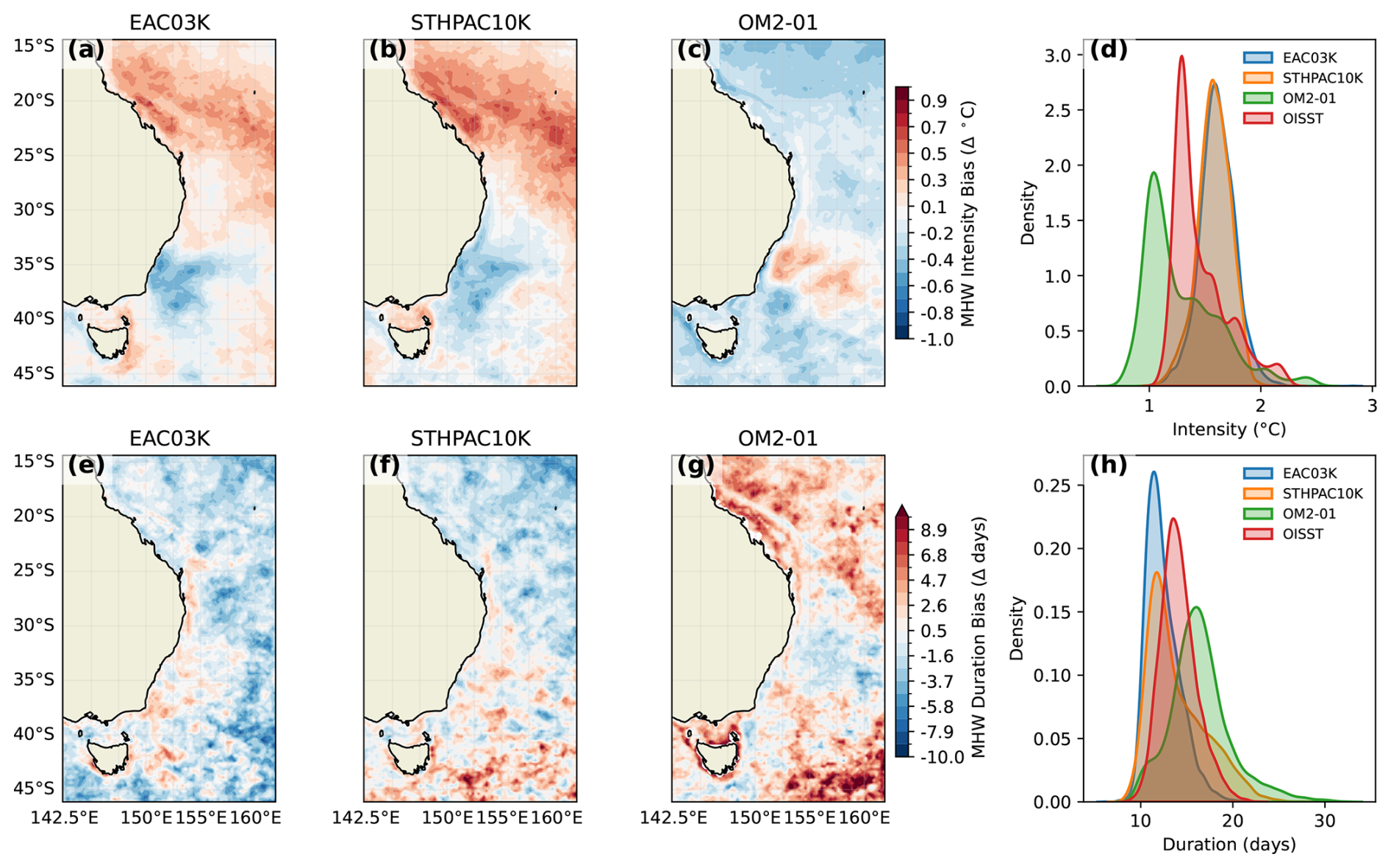
Figure 4 Surface marine heatwave results: (a–c) MHW mean intensity bias relative to OISST with (d) corresponding probability density function (PDF) of mean intensity per dataset (e–g) MHW mean Duration bias relative to OISST with (h) corresponding PDF.

Marine heatwaves (MHWs) are a key focal point for future use of the EAC03K model, hence it's important that this model not only represents the temperature variability, but also the presence of persistent extremes that arise in the satellite observations. Figure 4 summarizes the MHW results focusing on two key MHW metrics – mean intensity and mean duration. Figure 4a–c present the mean intensity bias averaged over all events at each grid point across the EAC domain. Here we see a similar spatial pattern to the SST variance bias (Fig. 3e) for the two regional models, which emerges as the broad north-west to south-east South Pacific convergence zone imprint of more intense MHW events than OISST produces. This is expected, given the intensity is essentially a derived metric from the SST variance, albeit relative to the daily-varying 90th percentile rather than the long-term mean (Hobday et al., 2016). Furthermore, there are noticeable differences in mean intensity for the separation and extension region. The regional models both have a coherent region of weaker intensities near the separation point (∼ 32° S) while the global model has higher intensities at the same location (Fig. 4a–c).

MHW durations are slightly shorter in EAC03K than STHPAC10K, particularly towards the south-east of the domain, while both models show longer-than-observed durations within the EAC system. The global model shows much longer durations throughout the domain as previously shown by Pilo et al. (2019). The spatially averaged probability density distributions (Fig. 4d, h) highlight the strong agreement between the two regional models, which consistently suggest higher mean intensities and shorter mean durations than the observational distribution. The global model shows broader distributions for both intensity and duration, while the peak of the distributions describe marine heatwaves that are less intense, and of longer duration than observations over the EAC model domain. This suggests that while the regional and global models may each align with observations at different times or under specific conditions, their inherent numerical differences prevent them from converging on a consistent representation of MHW characteristics.

We now assess the ability of each configuration to capture the temporal occurrence of MHWs. While MHWs in the region have a strong stochastic element due to the dominant control of the flow by mesoscale eddies (Cravatte et al., 2021; Chapman et al., 2025) we note that all configurations have identical surface forcing. As such, while individual events may be largely stochastic, we expect large-scale forcing to impact the general interannual variability in extreme events similarly across both OISST and the each simulation.

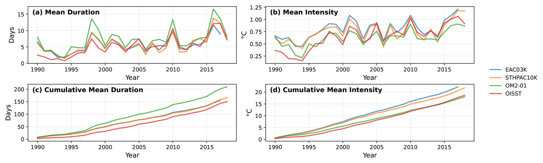
Figure 5 Spatially averaged MHW metrics: (a) mean duration; (b) mean intensity; (c) cumulative mean duration; (d) cumulative mean intensity.

We see a strong overall agreement between models and OISST in capturing interannual variability of MHW duration, with distinct peaks during strong El Niño years (e.g., 1998, 2010, and 2016) (Fig. 5a). As the probability distributions suggested (Fig. 4h), the two regional models agree strongly for the interannual MHW durations while MHWs in the global model tend to be consistently longer than observations across all years. Similarly, mean intensity patterns are broadly consistent across datasets, with a notable shift to higher intensities after 1994. The regional models generally produce more intense MHWs than the global model and observations, likely due to higher SST variance in the northern half of the domain (Fig. 5b). Interestingly, the 3 km model occasionally diverges from the 10 km model, such as in 2016, where it better matches observed mean durations. This suggests that resolution may play a more critical role during dynamically intense events, such as the advection-driven MHW of 2015/16 (Oliver et al., 2017). Overall, while model version differences dominate the results, resolution-specific effects emerge during periods of heightened dynamical complexity, highlighting the nuanced interplay between model numerics and resolution in simulating MHWs.

3.1.2 Regional Dynamics

All models show interannual variability in the poleward transports at the EAC jet zonal transect (Fig. 6a, c), and while the timing of enhanced (e.g., year 1998) and weakened (year 2000) transports track well between models, the magnitude of this yearly averaged transports differs substantially between the 3 and 10 km models (Fig. 6c). In the year 1998 for example, the yearly averaged transport for the 10 km models is between 15–18 Sv (1 Sv ≡ 10⁶ m³ s⁻¹) while for EAC03K, this peak reached 24 Sv. Although there are large interannual fluctuations in the modelled poleward transports, the long-term trend over the 30 year model runs appears relatively stable as shown by the dashed linear trend lines in Fig. 6c). The observational transports for the overlapping years with models shows similar magnitude to the 10 km models, while the EAC03K model produces transports weaker than observations in the first overlapping year (2012), and then transports almost twice as high for the year after (2013).

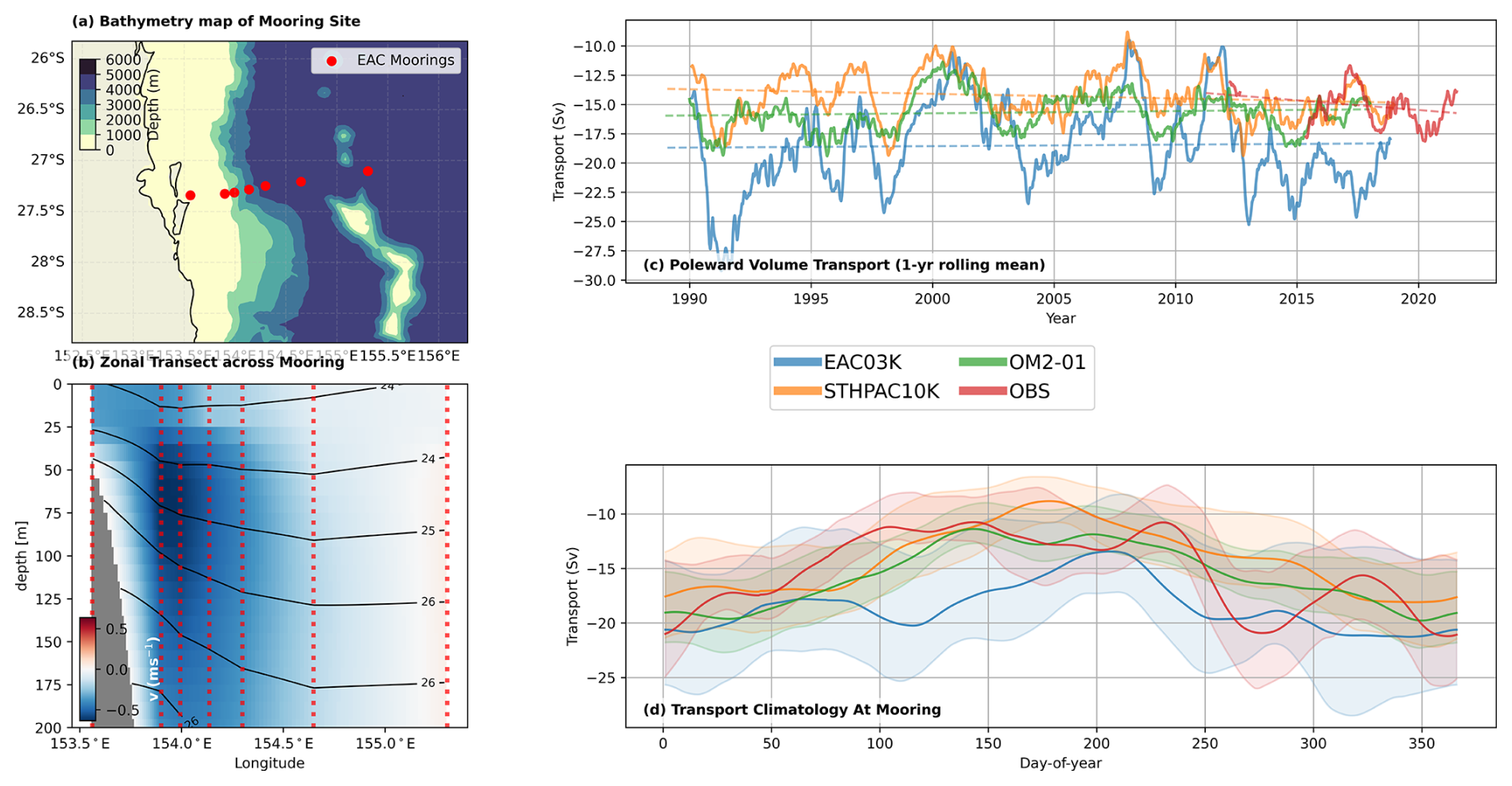
Figure 6 EAC jet full-depth southward transports at the EAC mooring array (∼ 27.3° S) – red transect in panel (a). (b) Zonal transect of long-term average meridional velocity from EAC Mooring Array with density layers in black and mooring locations in red; (c) 1-year rolling mean poleward transports at mooring site with linear trends as dashed lines; (d) daily-varying Climatological transport for all datasets.

The climatology of poleward transports in the EAC jet for all datasets is shown in Fig. 6d. All models follow observations with a poleward strengthening of transports in summer and a minimum in winter. The two 10 km models have very little variability around the daily-varying mean throughout the climatological year which allows for a clear seasonal cycle to be identified. The EAC03K climatology has a much higher sub-seasonal variability, however there is still an overall weakening in the winter months and strengthening in the summer. Interestingly, both the observations and EAC03K appear to have a two-stage strengthening from their winter minima whereby an initial rapid increase in transport is followed by a weakening before a second strengthening into the maximum summer peak. The timing of this sub-annual cycle is earlier for EAC03K than for the mooring observations by about one month. Nevertheless, the transition period is distinctly similar between the two configurations.

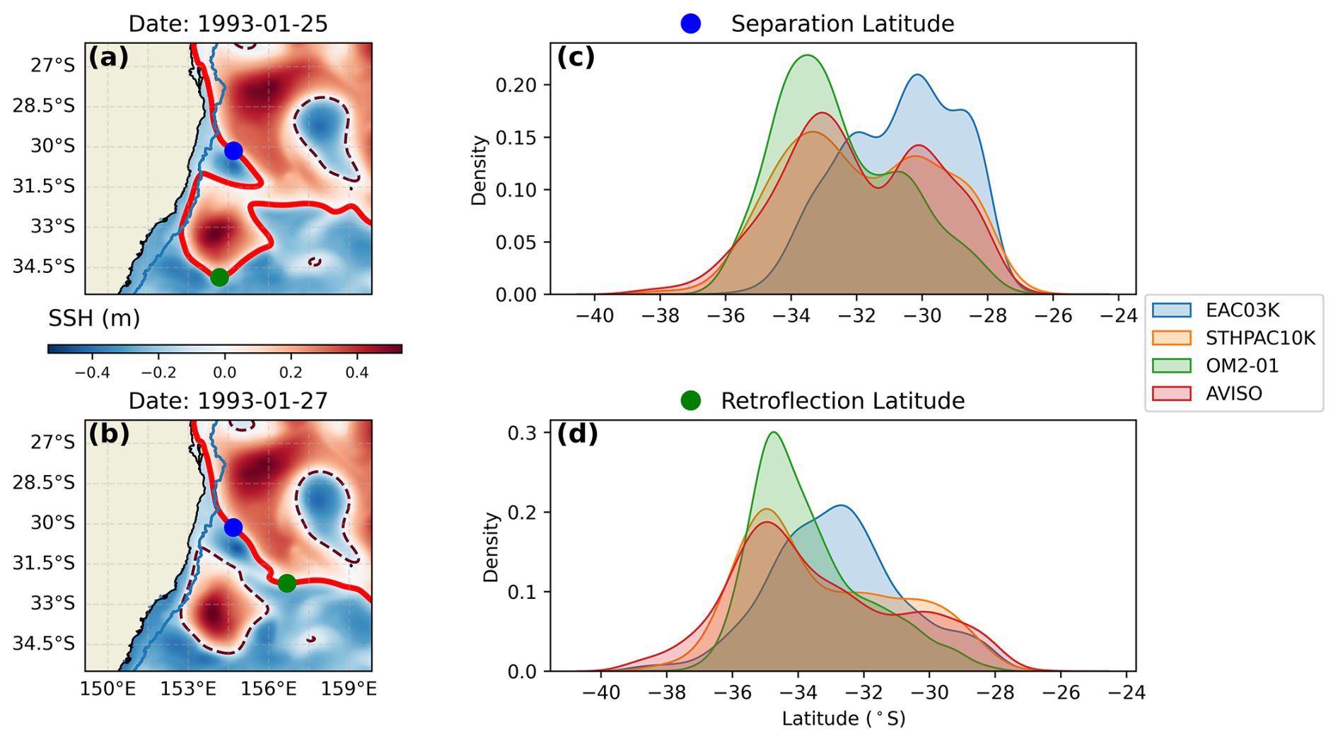
Figure 7 Separation and retroflection latitudes for all datasets. (a, b) Snapshots of SSH (shading) two days apart to highlight distinction between separation (blue dot) and retroflection (green dot) points. The red contour in panels (a) and (b) represents the chosen contour for detection. (c) PDF of separation latitude for all datasets; (d) PDF of retroflection point for all datasets.

Next we move south to the separation point of the EAC where our primary interest is understanding the latitude where the EAC jet separates from the shelf break, and additionally, where the main jet retroflects, i.e., where it changes direction from a poleward flow to a predominantly eastward or recirculating flow. The spatial maps in Fig. 7a, b demonstrate the typical case of the EAC before and after an eddy shedding event, and clearly demonstrate the importance of defining two distinct latitudes of interest for this region. Prior to eddy shedding (Fig. 7a), we have a separation point near 30° S and a retroflection much further poleward of 34.5° S. Two days later, after the eddy detaches from the main jet, we see little change in the separation latitude, while the retroflection latitude retracts equatorward by around 200 km. The separation latitude distribution of AVISO (Fig. 7c) shows two distinct peaks – a result previously reported by Cetina-Heredia et al. (2014). However, the exact locations of the peaks between that observed by our analysis (30.0 and 33.0° S) and that reported in their study (28.7 and 30.8° S) do indeed differ. Meanwhile, the retroflection point of AVISO in Fig. 7d has only a single peak two degrees of latitude below the poleward peak of the separation latitude at 35.1° S. The distinct difference between the separation and retroflection distributions of AVISO support the possibility that these critical points are governed by independent dynamics and forcing mechanisms – a finding not captured in earlier studies of the separation region, but one that may have important implications for the model behaviour explored below.

There is substantial difference between models in representing both the separation and retroflection latitudes. The global model, OM2-01, shows a tendency to separate toward the poleward (southern) extent of the latitudinal range, while STHPAC10K best represents the double peak distribution shape of AVISO (Fig. 7c). EAC03K separates much further north than the 10 km models and observations, and while there are occasions when it separates near the poleward peak of the observations, this rarely occurs. STHPAC10K captures the retroflection latitude distribution remarkably well, with a single peak and positively skewed tail (Fig. 7d). Similar to the separation latitude, EAC03K also shows an equatorward shift in the retroflection point relative to observationals and the 10 km models. These findings for the 3 km model support our earlier hypothesis that the positive SSH variance bias north of the typical separation region (Fig. 3o) could result in an earlier (equatorward) separation.

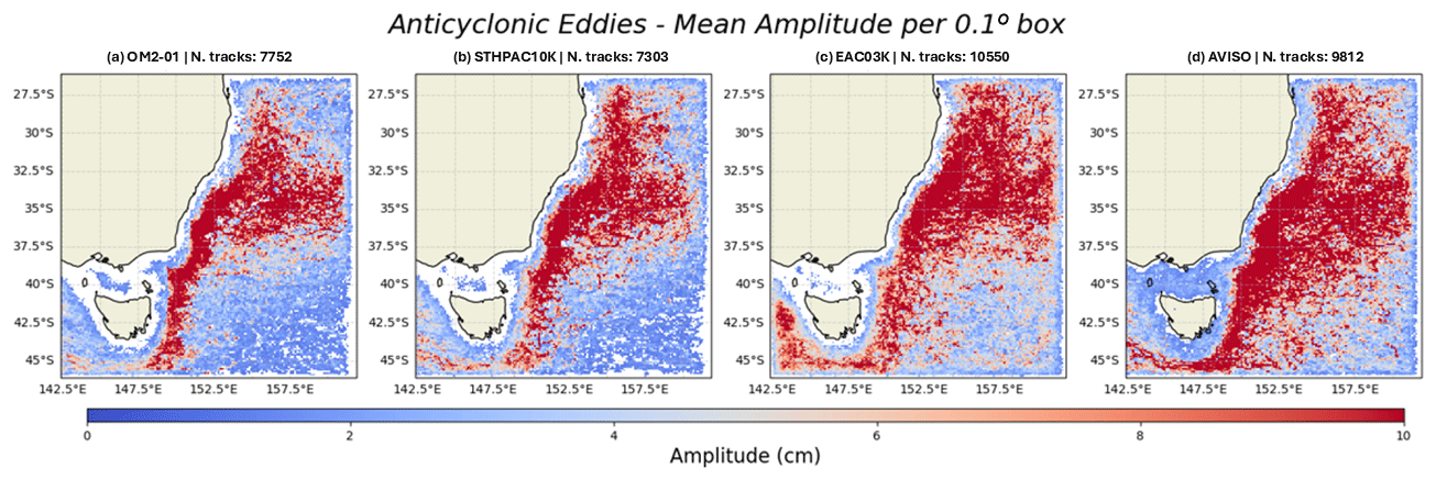
Figure 8 Mean eddy amplitudes for tracked anticyclonic eddies in all datasets.

The eddy tracking in the EAC extension has given us insight into the typical pathway of eddies and the amplitudes of these transient features that are critical to the heat transport along south-east Australia's nearshore region (Fig. 8). Here we focus specifically on anticyclonic eddies for the eddy tracking results. The 3 km model best reproduces the pathway and amplitude of anticyclonic eddies found in observations over the study period with a broad band of high amplitude eddies extending well below and to the south-west of Tasmania. The 10 km models capture the general pathway, however the band of high amplitude eddies is much narrower and eddies below Tasmania appear much weaker than in EAC03K and observations. Finally, the number of eddy tracks found in EAC03K (10 550 tracks) is much closer to that detected in the observational record (9812 tracks) while the 10 km models detected at least 20 % fewer anticylonic eddy tracks over the same period. The eddy tracking results suggest that EAC03K produces more high amplitude eddies than the 10 km models, highlighting the improvement gained from higher resolution when modelling geographical regions dominated by nonlinear turbulent ocean features. As above, these eddy-amplitude diagnostics are obtained from simulations using relative-wind stress, which is expected to suppress mesoscale kinetic energy to some degree through current feedback. Although this effect may itself vary with model resolution, it is not expected to substantially alter the qualitative differences shown here.

Australia's eastern continental shelf is exceptionally narrow, with some locations spanning less than half the width of a single 25 km resolution grid cell from the widely used observational datasets of AVISO and OISST. As a result, these global products do not resolve the sharp oceanographic gradients that define the shelf break, leading to a significant smoothing of critical nearshore features in addition to the well-known land contamination near coastlines. For this section we have introduced a new observational dataset, the IMOS-SST product at 2 km resolution (Griffin et al., 2017) which will provide further insight into the uncertainty between observational datasets and allow for more confidence when interpreting the differences between models and satellite-derived observations.

In this section we are primarily interested in assessing the agreement between models and observations in capturing the long-term SST trends along the shelf. We use the metric of relative warming in order to highlight regions that may be warming much faster than the global average, compared to those that might be warming on par with or slower than the global rate. This is a useful baseline, as it highlights regions where the ocean dynamics are changing, superimposing a localised ocean heat contribution onto the global SST warming trend.

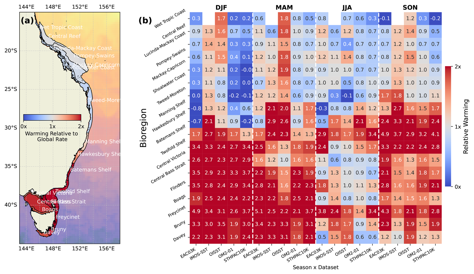
Figure 9 Sea surface temperature warming rates for coastal bioregions along eastern Australia relative to the global average warming rate over the past four decades. (a) Spatial map of labelled bioregions with shading representing the long-term annual SST trend across each polygon averaged over all datasets. (b) Heatmap of coastal bioregion warming relative to global average for all datasets across all seasons.

The broad SST warming patterns within the continental shelf bioregions of eastern Australia are presented in Fig. 9a. The shading, which shows the long-term average warming relative to the global average rate across all datasets for each bioregion, reveals a distinct shift between those upstream of the separation range, and those downstream. North of the Manning Shelf, the warming weaker than or equal to the global average rate. From the Manning Shelf and southward, the warming rates increase to well above twice the global SST trend. This supports previous work of Malan et al. (2021) which also find the coastal seas downstream of the separation point to be warming at twice the rate of those upstream.

Analysis of the bioregion SST trends by season and dataset (Fig. 9b) shows that the north/south contrast in warming rates are nuanced. Seasonally, regions upstream of the separation point show very little change across the year, while downstream, we see much lower warming rates in winter than all other seasons. This seasonal difference is particularly pronounced in the bioregions within Bass Strait, whereby winter warming rates are on par with global averages, while summer warming rates can be greater than three times the global rate. To further emphasize the local-scale differences in warming, bioregions directly adjacent to Bass Strait, such as the Freycinet bioregion show warming rates year-round that are around twice the rate as those in Bass Strait, e.g., Flinders bioregion. The winter cooling within Bass Strait is likely dominant over the continuous heat advected down the EAC extension during this season, while for locations more exposed to the EAC, weaker winter trends are less prominent (e.g., Freycinet).

The two observational products are largely in good agreement, apart from in spring and summer for bioregions within the latitude range of the typical separation point. During these two seasons, the IMOS-SST shows warming rates at least 1.5 times greater than the OISST product. The largest disagreement between models and observations occurs in summer for the upstream bioregions, whereby all models produce warming rates much slower than the global rate (shown by the blue shading), while the observations are close to or faster than the global average. In the downstream region, there is much less inter-model agreement, except in theFreycinet bioregion. EAC03K produces warming rates in autumn that are 5.1 times the global average rate, while the observations suggest relative warming rates of 2.5 and 2.2 for IMOS-SST and OISST respectively. This surprisingly large warming for the 3 km model raised some further questions as to the validity of this signal, which was also present in the surface biases presented in Sect. 3.1.

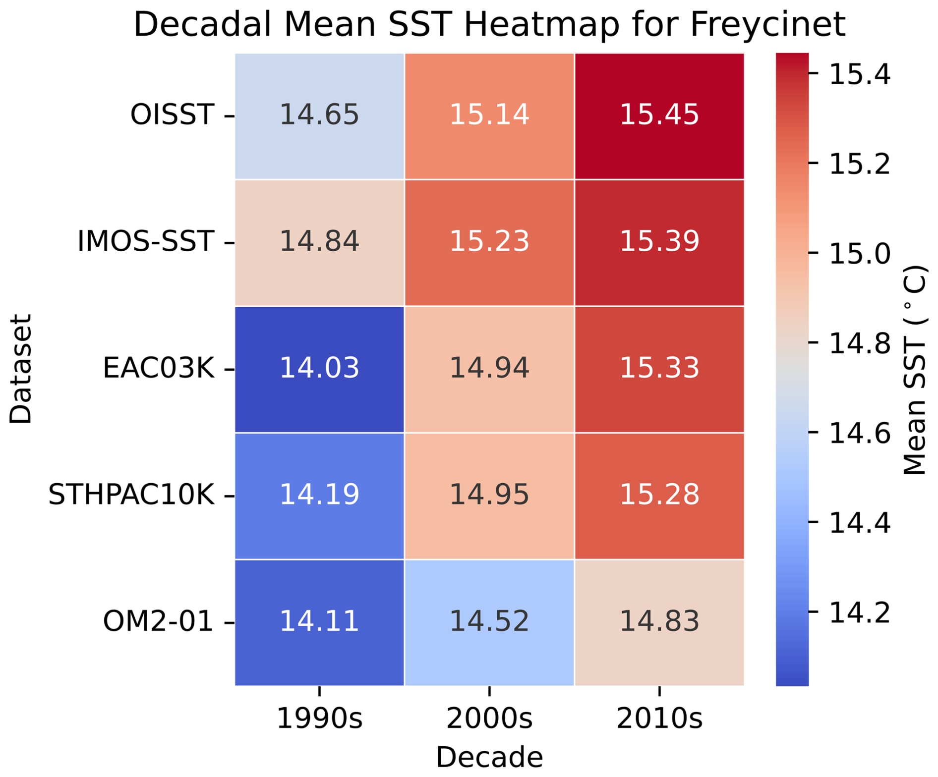
To further investigate the warming rate in the Freycinet bioregion, we analysed the average SST by decade across all datasets (Fig. 10), The 3 km model produces mean SSTs closer to the observed values for the last two decades than the global model, OM2-01. Hence, it is clear that although EAC03K is initially cold-biased in this region, as also identified in Fig. 3a, it adjusts and then better estimates the mean SST climate on the shelf of eastern Tasmania than the global model for the last two decades of the simulation.

Figure 10 Decadal Mean SST for the Freycinet bioregion shown in Fig. 9a.

3.2 Sensitivity Experiments

We tested the sensitivity to the initial conditions (ICs) by running a 10-year repeat-year-forcing (RYF) simulation over the EAC03K domain and taking the ICs for all sensitivity experiments from the 10th year of this RYF run. Subsequent comparisons between RYF-ICs and the ICs taken directly from the forcing dataset (IAF runs) showed no substantial changes in global metrics (not shown). We conclude that it makes little difference whether the IAF run is initiated from a 10-year RYF spin-up or from an IAF snapshot of the forcing model. However, all sensitivity experiments are initiated from the 10-year RYF spin-up (RYF-ICs).

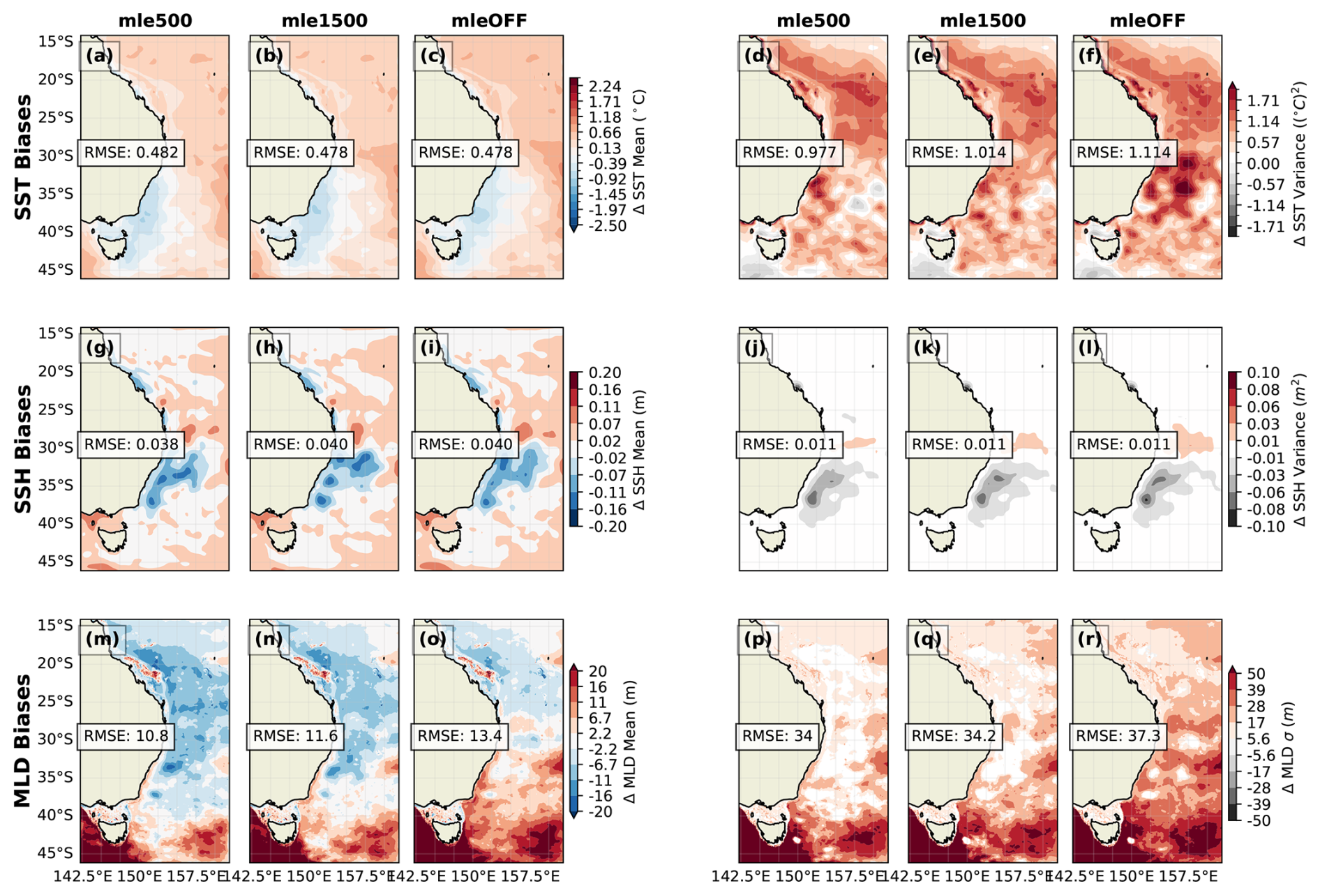
Figure 11 MLE Sensitivity Biases for SST (a–f), SSH (g–l) and MLD (m–r) while long-term (10-year) mean bias are presented in the left column, and long-term variance bias are presented in the right column. Note that negative mean biases here indicate shallower modelled MLD, while positive biases indicate deeper MLDs.

Both increasing the MLE parameter value from 500 to 1500 m, and further turning the MLE scheme off, have little effect on the mean and variance of SST and SSH (Fig. 11a–l). Given Adcroft et al. (2019) and Ross et al. (2023) both highlight the sensitivity of SST biases to the MLE scheme, this was a surprising result and indicates the potential redundancy of MLE parameterization at 3 km horizontal resolution. The mixed-layer depth (MLD) does show more sensitivity to the MLE scheme. With a parameter value (frontal length) of 500 m (Fig. 11m), there is a negative bias over much of the EAC domain, while the southern boundary has substantial positive mean biases exceeding 20 m in some areas. When the MLE scheme is slightly relaxed to a frontal length of 1500 m, the overall effect is to reduce the shallow mean bias in mid-latitudes, but increase the area of deep MLD bias south of about 30° S. With the MLE parameterization turned off, there is a substantial decline in negative mean MLD bias, and an overall growth in the positive mean MLD bias in the southern half of the domain. A similar pattern is observed with the MLD variance; a region in the south of large variability in the MLE500 experiment, extends northward with the MLE1500 experiment, and then extends over the entire domain for the MLE-OFF experiment (Fig. 11p–r). Hence it is clear that relaxing the MLE parameterization both deepens the mixed layer, and produces more variability. However, given the minimal effect on the surface properties and the range of uncertainty associated with the MLD observational dataset, this suggests the 3 km model is quite robust to the parameterization choice for mixed layer instabilities.

A surprising result from the VISC experiments is the strong agreement between the VISC-H (high viscosity) and AVISO for separation and retroflection latitudes that was not seen in the earlier EAC03K simulation (Fig. 7). Noting the only difference between VISC-H and the nested EAC03K configuration is the boundary forcing dataset (STHPAC10K for EAC03K, and OM2-01 for VISC-H), we can therefore conclude that there is clearly a sensitivity to the boundary conditions for the 3 km model. Further investigating the cause of the poor agreement when forcing this model with the large-regional model is outside the scope of this study. It is nevertheless important to highlight this discrepancy and furthermore, surprising to note the now strong agreement between the 3 km model with high viscosity, and the AVISO results.

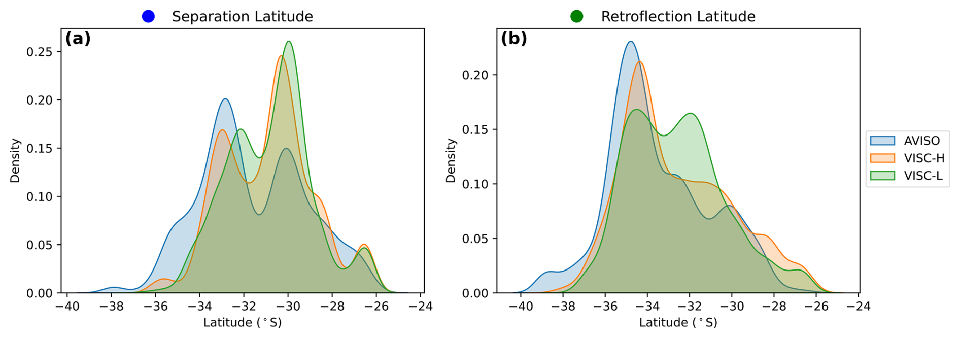
Figure 12 (a) Separation latitude and (b) retroflection latitude probability density distributions for the VISC experiments.

The separation latitude distribution of the low-viscosity (VISC-L) experiment is remarkably similar in shape to VISC-H, however its peaks are shifted northward by up to 100 km (Fig. 12a). VISC-H shows strong agreement with the observed retroflection distribution, with a single peak between 35–36° S, and a positive skew toward the north of the range (Fig. 12b). Interestingly, VISC-L exhibits two peaks, resembling observed separation latitude moreso than the observed retroflection distribution shape. This demonstrates vastly different behaviour in the retroflection latitude for VISC-L compared to the VISC-H simulation. It is clear that the original viscosity parameter value used in VISC-H best suits the observed distributions of both the separation and retroflection.

4 Discussion

This paper has evaluated a MOM6 regional model suite nested within a global MOM5 configuration, for the simulation of the East Australian Current region and adjacent Coral and Tasman Seas. We have also assessed the sensitivity of a submesoscale-permitting regional model to sub-grid parameterizations and boundary forcing. In doing so we have made several modelling and scientific contributions that will be discussed in more detail below. Key modelling results include the improved representation of eddy characteristics along the EAC extension pathway and Tasman Outflow and also the demonstrated influence of weaker viscosity on WBC separation dynamics within the model. Importantly, we have also presented evidence for a redundancy of the Mixed-Layer Eddy parameterization in a 3 km resolution ocean model, suggesting that the restratification effects of mixed layer instabilities are at least partially resolved at this resolution. The scientific results include the novel definition for separation and retroflection latitudes and how these points differ dynamically, and also the improved understanding of temperature trends along the entire eastern Australian continental shelf. Ultimately we are still left with biases in our model suite that are not explained by the sensitivity tests we have carried out. However these do not have any overwhelming detrimental influence on the key dynamical features of the EAC system in our 3 km model.

4.1 Horizontal Resolution

We anticipated that a higher resolution would lead to improved representation of the nonlinear dynamics of the EAC extension eddy field based on the argument of the first baroclinic deformation radius being well resolved at higher latitudes in our 3 km resolution model compared to the 10 km resolution models (Fig. 2b). This does indeed appear to be the case in our eddy tracking results, which show that high amplitude eddies at 3 km resolution retain their structure along the southward path of the EAC extension and on through the Tasman Outflow (Pilo et al., 2015). Additionally the broad spatial extent of high amplitude eddies at 3 km aligns much more closely with that of the observations, while the 10 km models have a much narrower meridional band of high amplitude eddies close to the coast. Li and Roughan (2023) identified baroclinic instability as the dominant energy source for mesoscale eddies in the southern EAC extension region, which is a process with energy injection scales close to the first baroclinic Rossby radius (Cushman-Roisin and Beckers, 2011). As the 10 km models do not well-resolve this length scale, particularly in the more poleward extent of the domain, we indeed see weaker simulated eddy amplitudes with respect to the observed results for the coarse models, while the 3 km model truly resolves this baroclinic energy conversion process. This result presents a clear case for truly resolving the mesoscale energy spectrum in order to accurately represent nonlinear eddy dynamics in regions of high baroclinic instability.

While it is clear that resolving smaller length scales can improve the representation of eddies compared to observations, the opposite is evident regarding EAC separation and retroflection latitudes. The earlier boundary current separation and retroflection in the EAC03k model was associated with the open boundary forcing from STHPAC10K – likely introducing more instability in the upstream jet – and it was shown in the sensitivity experiments, that forcing EAC03K with OM2-01 indeed remedied this issue. This result highlights the higher sensitivity of model behaviour when we are moving to finer horizontal grids and also the sensitivity to the open-boundary forcing data.

The 3 km model exhibits strong SST biases off eastern Tasmania, showing a colder mean temperature and a faster warming trend compared to observations and 10 km models. These biases are partly linked to the slower equilibration of EAC03K in the highly nonlinear EAC extension region. Li and Roughan (2023) showed that baroclinic processes dominate the local energy balance off south-east Australia, and these processes act on inherently slower timescales than the more barotropically dominated northern extent of the EAC extension. Furthermore, because the high-resolution model resolves a wider range of active spatial scales, energy must cascade across many more degrees of freedom. As a result, additional eddy turnover times are required for the system to reach a quasi-equilibrated turbulent regime (Smith and Vallis, 2001). The nearshore temperatures in EAC03K show a similar cold start before converging on observed temperatures for the latter two decades of the simulation, providing confidence in the equilibrated ocean state in this region for the later period. Future work will focus on the scales and efficiency of energy flow in the turbulent EAC extension region, comparing the interannual variability in mesoscale energy between the models developed for this study.

An important limitation of the present ocean-only framework as opposed to a coupled ocean-atmosphere model is the use of relative-wind stress in combination with a prescribed atmospheric forcing. By including the surface current in the bulk momentum flux, this formulation accounts for wind-current interaction, but it also tends to reduce wind work on the mesoscale circulation and damp eddy kinetic energy relative to direct-wind forcing (Renault et al., 2016). This should be kept in mind when interpreting absolute SSH variance, and eddy-related diagnostics. Nevertheless, because the same stress formulation is used consistently across the configurations analysed here, the comparative differences reported in this study remain informative, even though the absolute level of mesoscale variability may depend in part on the chosen wind-stress formulation.

4.2 EAC03K Sensitivities

We will now discuss what we have identified as the most important considerations for configuring a higher resolution model based on the presented evidence and experience gained through the sensitivity experiments in this study.

Firstly, the separation latitudes measured in the EAC03K model matched better with observations when forced with OM2-01 at the boundaries rather than with STHPAC10K, the latter resulting in an unrealistic earlier separation of the WBC (Figs. 7 and 12 respectively). This result was surprising, given STHPAC10K improves on OM2-01 in many ways including improved agreement with AVISO for the separation/retroflection latitudes. The tendency for an earlier separation of the WBC indicates that the upstream jet is too unstable within the simulation forced by STHPAC10K. This result underscores the importance of considering the quality of the forcing datasets at the boundaries.

Relaxing the MLE parameterization had the expected effect of deepening the mean mixed layer and increasing its variability, similar to the changes outlined by Fox-Kemper et al. (2011) and Ross et al. (2023). Although it was hoped that this sensitivity test might explain the band of high SST variance bias across the northern half of the domain in both MOM6 regional models (Fig. 3), it had no effect on the SST mean or variance in this region. This was surprising as Adcroft et al. (2019) reported a strong sensitivity in SST with biases to the MLE parameterization under different frontal length scales in their $\mathrm{1}/\mathrm{4}$ and $\mathrm{1}/\mathrm{2}$° global configurations. Although only a very broad evaluation has been conducted here, results suggest a 3 km resolution model may partially represent the mixed layer instabilities required to break down the Rossby-adjusted mixed layer fronts in the EAC domain – a mechanism well described by Boccaletti et al. (2007). Similar to the Gent-McWilliams mesoscale parameterization scheme being turned off for resolutions that do not fully resolve the mesoscale, perhaps the Fox-Kemper MLE restratification becomes unnecessary at scales that partially resolve the submesoscale (i.e., 3 km resolution).

Through the novel definition and algorithmic improvement in detecting the separation and retroflection latitudes of the EAC, we have identified semi-independent dynamics governing the latitude where the EAC first separates, and where the main current veers eastward. The distinctly different PDFs of the two latitudes, consistent across both observations and models, suggest that they are indeed semi-independent. The initial separation tends to occur at two preferred latitudes, previously shown to align with key geographical locations where the continental shelf narrows (Cetina-Heredia et al., 2014). The retroflection predominantly occurs further downstream at a relatively stable latitude, largely independent of where the topographic separation takes place. This suggests both points likely have a flow-dependent component – as indicated by the variability around the PDF peaks, while the separation point is influenced more by topography, and the retroflection point more by the basin-scale external forcing.

The viscosity experiments further highlight the differences in dynamics governing the separation and retroflection points of the EAC jet. Weakening the imposed viscosity results in a linear shift in the PDF for the separation point whereby the entire distribution migrates ∼ 100 km equatorward. This suggests the two peaks are still associated with the topography, while the lower viscosity leads to faster/earlier response of the current to instability growth. The retroflection PDF exhibits a nonlinear response to weaker viscosity indicated by the change in the PDF from a single positively skewed distribution, to a double peak, more similar to the separation PDF in shape. This shift towards a co-varying response between the separation and retroflection at lower viscosity indicates a change in the governing dynamics of the retroflection, from an externally forced (wind stress) response, to a topographic response, simply due to a weaker viscosity allowing faster instability growth. We have shown that the larger viscosity coefficient produces a more realistic WBC separation, while also highlighting the distinct forcings associated with the separation and retroflection latitude ranges and how that changes under a lower viscosity simulation.

There were substantial differences between the MOM5 (OM2-01) and MOM6 (STHPAC10K) simulations, both in surface metrics and region-specific evaluations. Interestingly, the 10 km regional model (STHPAC10K) often showed greater similarity to the 3 km regional model than to its global counterpart, despite the 3 km model having widely different boundary locations. This suggests that the open boundary conditions are not the dominant source of bias in the regional simulations. If boundary effects were the primary driver, we would expect significantly different bias patterns between the two regional models. Instead, the biases in the EAC region are large, coherent, and consistent across both regional configurations, indicating that their source lies elsewhere.

Given that OM2-01 and STHPAC10K share identical horizontal and vertical resolution, forcing, and bathymetry, the differences between them must stem from the fundamental difference between MOM5 and MOM6. However, it is not immediately clear whether MOM6 systematically outperforms MOM5 in this region under the given forcing and parameter set. While some biases in STHPAC10K are weaker than those in the global model, others are of opposite sign and/or even larger in magnitude (e.g., SST variance, MHW intensity). These findings reinforce that MOM6 introduces notable changes compared to MOM5, many of which remain underexplored in the context of regional ocean dynamics.

5 Conclusions

We have developed and assessed two new regional ocean models to investigate the influence of the East Australian Current on the adjacent shelf seas of eastern Australia. While our primary goal was to evaluate the skill of a high-resolution 3 km ($\mathrm{1}/\mathrm{30}$°) model in capturing the large-scale variability of the EAC, our analysis also revealed important sensitivities of the regional MOM6 model to boundary forcing, physical parameterizations (e.g., the Fox–Kemper MLE scheme), and numerical closures (dynamic viscosity) that extend beyond the initial scope of the study. We found that the 3 km model more faithfully represents the nonlinear dynamics (mesoscale eddies) of the EAC extension than the 10 km models, whereas in the upstream quasi-linear region the meso-to-large scale structure is adequately resolved at 10 km resolution, offering limited added value from further grid refinement. Overall, the 3 km model demonstrates clear fitness for purpose in reproducing the meso- and large-scale dynamics of the EAC system, while highlighting the limitations of coarser (10 km) models in representing the complex, nonlinear variability that governs the EAC extension and its interaction with the adjacent shelf.