Representing canopy structure dynamics within the LPJ-GUESS dynamic global vegetation model (revision 13221)

The competition, especially for light, is a fundamental determinant of the structure and composition of a forest. Large-scale forest models must balance real-world complexity with computational demand and poorly constrained parameters. The LPJ-GUESS dynamic global vegetation model has a strong track record of simulating forest composition and tree demography with a simple representation of forest canopies. However, its current approach is limited in its ability to explore the functional coexistence of trees within forest patches or to represent the full implications of forest management actions that create heterogeneous light conditions on the forest floor. This is because LPJ-GUESS currently represents forest canopy light transmission with vertically overlapping crowns, neglecting any horizontal structural heterogeneity. Whilst computationally efficient, this scheme does not allow for a realistic representation of light distribution on forest floor following tree death or harvest.

Here we describe the implementation of a new scheme with spatially explicit canopies, where tree cohorts have a fixed position within a patch, enabling simulation of forest floor light conditions that better captures spatial variation, especially following disturbances such as tree death or harvest. Additionally, we test a lower-complexity canopy scheme based on the perfect plasticity approximation.

To evaluate these developments, we conducted four assessments. First, we evaluated the model's performance against field observations of aboveground woody biomass, mortality, and productivity across diameter size classes. Second, we examined their ability to represent tree functional coexistence. Third, we explored how forest harvest influenced the re-establishment of a woody understory. Lastly, we conducted two sensitivity tests.

Results show that the spatially explicit canopy scheme improves the representation of forest tree size structure and dynamics across boreal, temperate, and tropical regions. It enables functional coexistence without the influence of large-scale disturbances, captures the interplay of forest gap dynamics with the establishment of a recruitment layer, and produces more realistic understory light environments and competitive interactions, capabilities not achievable with the standard canopy scheme. By capturing these dynamics without requiring explicit individuals, the scheme expands methodological options for bridging individual-based and cohort-based models, while avoiding abrupt canopy-layer transitions and enabling a more gradual and ecologically consistent representation of canopy reorganization. This improves the representation of stand structure and key demographic processes, enhancing the model's capacity to simulate forest dynamics, resource fluxes, and responses to environmental change, while improving alignment with observational data.

1 Introduction

Forest demography is the study of how tree populations change over time through processes such as recruitment, growth, and mortality. From these processes emerges a complex mosaic of individual trees of different size, age, and species. The emergent forest structure and composition then govern its capability to react to environmental changes, disturbances, and climate variability (Waring and Running, 2010). A correct representation of forest structure and demographic processes are therefore crucial for forecasting ecosystem services like carbon sequestration, biodiversity, and resilience to extreme events and disturbances (Brockerhoff et al., 2017; McDowell et al., 2020).

One of the primary drivers of forest dynamics is competition, whether for light, water, or nutrients, which shapes the structure and composition of vegetation within a forest. The vertical and horizontal distribution of trees within the forest canopy determines how photosynthetically active radiation (PAR) is partitioned, influencing the growth and productivity of different trees and other forest species. Taller trees typically absorb more light, overshadowing shorter trees in the understory and, thus, affecting their growth, survival, and succession (King, 1990; Niinemets and Kull, 1995). Not only does the vertical distribution of trees within the canopy play a crucial role, but spatial interactions in general. As neighbouring trees compete for resources, their spatial arrangement determines their individual success, as well as the overall structure and function of the forest (Pacala and Deutschman, 1995; Kunstler et al., 2012). Physical arrangements and interactions result in the establishment of spatial heterogeneity, supporting the creation of canopy gaps, which allow light to reach various forest layers, facilitating species coexistence, succession, and the promotion of biodiversity by generating diverse micro-environments (Brokaw and Busing, 2000). Beyond that, disturbances, ranging from individual tree mortality to large stand-replacing events, further shape forest structure and composition (Hardiman et al., 2013). The dynamic interplay between light availability, stand structure, and disturbance regimes drives ecological processes such as species interactions and forest succession. Such processes, in turn, influence ecosystem resilience, helping forests recover from disturbances and maintain their ecological function.

To understand this complex interplay of forest dynamics, demographic modelling is a critical tool to advance our understanding of forest ecology (Lavorel and Garnier, 2002). Through the simulation of vegetation demography, we can gain insights into plant population interactions, ecosystem health, and resilience, as well as better predict environmental responses and inform sustainable forest management strategies (Sitch et al., 2008). In recent years, various approaches have been developed to model forest dynamics, striving to balance model fidelity with its complexity (Shugart, 1984; Moorcroft et al., 2001; Strigul et al., 2008). Vegetation demographic models (VDMs) are powerful tools for generating ecological forecasts, as they simulate the complex interactions between plants, climate, and both biotic and abiotic factors. These models typically incorporate key processes such as photosynthesis, respiration, as well as carbon, nutrient, and water cycling, all of which are essential for capturing the complex functioning of ecosystems (Fisher et al., 2018). By resolving demographic processes, VDMs can represent how plant populations respond to internal dynamics (e.g. establishment, growth, and mortality) and external drivers such as climate change, land-use change, management or natural disturbances. One such model, LPJ-GUESS, has represented forest demography for over 25 years. LPJ-GUESS uniquely combines an individual- and patch-based representation of vegetation dynamics with ecosystem biogeochemical cycling, making it well-suited for simulating forest structure, species composition, and demographic processes (Smith et al., 2001, 2014).

Over the years, LPJ-GUESS has proven to be highly capable of modelling forest ecosystem processes. The representation of vegetation composition and structure is achieved by grouping tree individuals based on their plant functional types (PFTs) and age classes into cohorts, which represent groups of trees with similar ecological characteristics. Individual trees within a cohort do not compete among themselves for light, as they are assumed to be perfectly aligned, with the total crown area representing the sum of all individual tree crown areas in the cohort. For resources such as water and nutrients, all individuals within a cohort are assumed to experience the same level of limitation, if any, and therefore do not compete among themselves. Competition for essential resources such as light, water, nutrients, and space only occurs between cohorts within the modelled area (patch). By simulating the competition between cohorts of different PFTs and age classes, LPJ-GUESS captures changes in forest structure and composition over time, especially in response to stand-replacing disturbances (Hickler et al., 2012; Smith et al., 2014; Pugh et al., 2024). Such simulations reflect natural forest succession, where cohorts of fast-growing, shade-intolerant and early successional PFTs occupy open areas, rapidly generating shade that suppresses their own seedlings. As the forest matures, the environment becomes more conducive to the establishment of shade-tolerant, late successional PFT cohorts.

To account for the stochastic nature of ecological processes and the inherent heterogeneity of the landscape, LPJ-GUESS simulates multiple replicate patches per grid cell, each evolving independently to capture variability in processes such as establishment, mortality, and disturbance, processes that in turn shape vegetation composition, structure, and forest dynamics, including age structure and productivity. As an example, LPJ-GUESS simulates how changes in disturbance regimes, such as shifts in the frequency of stand replacing events, influence the forest carbon sink, either increasing or decreasing it depending on disturbance return times and forest type (Pugh et al., 2019b). Also, the simulation of fire regimes and their impact on forest demography provides valuable insights into how changing fire frequencies influence forest composition and structure (D’Onofrio et al., 2020). Furthermore, LPJ-GUESS incorporates nutrient limitations, which are critical in shaping forest composition and structure. When simulating boreal forests, for instance, alleviating nutrient limitations on productivity could lead to forest densification in a warmer future climate (Wårlind et al., 2014). All in all, these capabilities make LPJ-GUESS a versatile tool for simulating forest dynamics in response to a wide range of ecological and environmental factors.

While LPJ-GUESS has proven successful in modelling dynamic forest responses thanks to representing demography, the increasing availability of observational data has revealed some limitations in the model pertaining to capturing finer-scale processes (Pugh et al., 2019b; Dietze et al., 2018; Van der Plas et al., 2018). For instance, the model relies on stand-replacing disturbances as proxies for all types of disturbances, which is an oversimplification that leads to the under-representation of vertical forest structure shaped by smaller-scale disturbances, which are more common in reality. As a consequence, it struggles to accurately represent tree size distribution and species composition, when assessed at a small scale. Moreover, the model tends to simulate a persistent dominance of late-successional PFTs in old-growth forests, which may overlook the ongoing compositional changes and structural complexity present in many natural forests. While such dominance has been documented in certain systems (Brzeziecki et al., 2020), numerous old-growth forests continue to exhibit dynamic and diverse community structures over time (Waterman et al., 2020). Incorporating horizontal variability within forest ecosystems is another crucial consideration. For example, LPJ-GUESS has difficulties in simulating regeneration patterns after small scale natural mortality and harvest events, where pioneer PFTs should rapidly colonise newly created small gaps. Pacala and Deutschman (1995) demonstrated that mean-field models, i.e. models which often ignore horizontal heterogeneity within a patch, can underestimate basal area by as much as 50 % compared to models that account for spatial variability, underscoring the importance of integrating horizontal patchiness into forest demographic simulations.

These shortcomings might be less relevant for large tropical trees but become important for the majority of trees, which have much smaller crowns than the patch size, particularly during forest regeneration. This highlights the need for further improvements in the model’s canopy structure representations, which are central to simulating small scale forest dynamics. Currently, LPJ-GUESS distributes each cohort’s leaf area evenly across the entire patch, disregarding the actual crown area, which results in a horizontal uniform light distribution over the patch. This uniformity prevents the formation of light gaps, hampering regeneration and species coexistence. To address the above issue, we have developed a new light transmission scheme called the “spatially-explicit canopy” (SEC). This novel scheme aims to provide a more accurate representation of the horizontal canopy structure, particularly in the absence of large disturbances, as well as to enhance species coexistence and allow simulation of the re-establishment of shade-intolerant PFTs in relatively small canopy gaps following individual tree mortality or harvest events.

In this paper, we present a detailed description of the spatially-explicit canopy scheme, SEC, and evaluate its performance in several key areas. We (1) evaluate its ability to capture stand structure and dynamics using data from forests around the world; (2) assess its improved representation of functional coexistence, here defined as the persistence of multiple PFTs within a single patch; (3) examine how sensitive the simulated re-establishment is to different harvest intensities, as a proxy for gap size; and (4) test the scheme’s responsiveness to key parameters, such as wood density, establishment rates, and mortality.

2 Methods

2.1 Model description

Historically, LPJ-GUESS (Smith et al., 2001, 2014; Sitch et al., 2003) employed a “vertically overlapping crowns” approach to represent canopy structure (Fig. 1a). This approach is referred to as LPJ in this context. In the LPJ canopy structure scheme, horizontal spatial structure within a patch was not considered for light absorption. Instead, the scheme represents canopy structure purely in the vertical dimension, using cohort bole and total height derived from pipe model-based allometric relationships (Shinozaki et al., 1964a, b; Waring et al., 1964; Smith et al., 2001, 2014). The actual crown area was not directly accounted for, as the leaf area of each cohort was assumed to be uniformly distributed both horizontally across the patch and vertically through the canopy, resulting in a well-mixed leaf distribution.

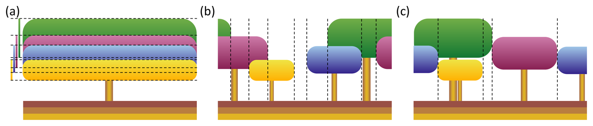
Figure 1 Canopy structure representation of four tree cohorts in a single LPJ-GUESS patch. (a) Standard LPJ-GUESS (LPJ) – in this scheme, the canopy lacks a heterogeneous horizontal structure. The leaf area is evenly distributed across the entire patch, and the canopy structure is determined solely by the tree and bole height of each cohort. In this example, the canopy has a single horizontal section with seven distinct vertical sections in which light absorption needs to be calculated. The bars on the left visualise the depth of each cohort's canopy. (b) Spatially-explicit canopy (SEC) – cohorts have fixed positions within the patch. When an individual tree within a cohort dies, the cohort’s total crown area is reduced, a gap may be created in the canopy. This gap persists over time, allowing new cohorts to establish and grow under full light conditions. This example has nine vertical sections, the outer sections being identical, whose individual light conditions are determined in a similar manner as in (a). (c) Perfect plasticity approximation (PPA) – cohorts are organised by tree height, filling the patch area perfectly. The tallest tree cohorts fill the patch until the cumulative crown area equals or exceeds the patch area. Once the patch is filled, an understory layer is formed by the next shorter tree cohort. This example has five distinct vertical sections.

The fraction of incoming PAR (fPAR) absorbed by each cohort was calculated using the Lambert-Beer law (Prentice et al., 1993; Smith et al., 2001), which assumes that cohorts shade themselves and the cohorts beneath them

$$\begin{array}{}\text{(1)}& \text{fPAR}\left(z\right)=\mathrm{1}-e^{-k\text{LAI}\left(z\right)}\end{array}$$

where fPAR(z) denotes the fraction of PAR at canopy depth z (m), k is the light extinction coefficient, and LAI(z) is the summed leaf-area index (LAI; m² m⁻²) of leaves from all cohorts above canopy depth z. For canopy sections with more than one cohort, fPAR was distributed among the cohorts based on each cohort's LAI fraction in that section, assuming that all cohorts shared the same extinction coefficient (k). For the canopy illustrated in Fig. 1a, this resulted in seven distinct vertical sections that needed to be calculated to determine each cohort's fPAR. The remaining fPAR (fPAR_herb,top) becomes available on the forest floor for absorption by the herbaceous understory. The total annual forest floor PAR (PAR_est; $\mathrm{J}{\mathrm{m}}^{-\mathrm{2}}{\mathrm{d}}^{-\mathrm{1}}$) then determined whether the light conditions were sufficient for a specific PFT to establish and influenced both the biomass and the number of newly established saplings. The minimum light condition (PAR_est,min; $\mathrm{J}{\mathrm{m}}^{-\mathrm{2}}{\mathrm{d}}^{-\mathrm{1}}$) required for fast-growing, shade-intolerant pioneer PFTs was higher than that for slow-growing, shade-tolerant PFTs. In the LPJ approach, the uniform distribution of each cohort's leaf area across the entire patch ensured that there were no canopy gaps that allowed full light to reach the forest floor, as long as at least one tree cohort was present. Consequently, consistent shading provided an advantage to slow-growing, shade-tolerant PFTs, as the forest floor remained constantly shaded. Instead of representing actual canopy gaps, the LPJ scheme simulated canopy gap dynamics by using a large set of replicate patches. Each patch faced a patch-destroying disturbance with a probability corresponding to an average return interval of 100 years (Smith et al., 2014; Pugh et al., 2019a). In this study, we examined the effect of this patch-destroying disturbance by having it turned on (LPD) and off (LPJ). Another issue with uniformly distributed leaf area across the patch was that in a patch containing a single tree cohort, where its total crown area (CA_i; m²) only covered a fraction of the patch, the fPAR of that cohort was overestimated, according to Eq. (1), compared to if the cohort's leaves only covered its actual crown area. This occurred because the leaves were spread over a larger area, resulting in less self-shading than what would occur with a more realistic crown area. Consequently, this could lead to an unrealistically low tree density (under-crowding). In highly productive sites, a single large cohort with high LAI could potentially shade all shorter cohorts to the point of death caused by reduced growth efficiency. This can occur even if the taller cohort’s CA_i covers only a fraction of the patch. Conversely, over-crowding could occur because the CA_i did not limit tree density in a patch unless CA_i of an individual cohort exceeded its maximum available crown area (CA_max,i; m²), which corresponded to the entire patch area (0.1 ha) in LPJ. Self-thinning was triggered only when ${\text{CA}}_i>{\text{CA}}_{\text{max},i}$, implemented as an increased probability of mortality (mort_self); otherwise, no self-thinning occurred (Eq. 2). This self-thinning response was determined solely by the crown area of the individual cohort and did not depend on the total crown area of all cohorts within the patch.

$$\begin{array}{}\text{(2)}& {\text{mort}}_{\text{self}}=\left\{\begin{array}{ll}\mathrm{0}& {\text{CA}}_i\le {\text{CA}}_{\text{max},i}\\ \frac{{\text{CA}}_i-{\text{CA}}_{\text{max},i}}{{\text{CA}}_i}& {\text{CA}}_i>{\text{CA}}_{\text{max},i}\end{array}\right.\end{array}$$

To overcome limitations of the LPJ approach associated with its lack of horizontal spatial structure, the new SEC canopy scheme was introduced. In SEC (Fig. 1b), the centroid of a cohort’s aggregated crown area, representing the combined crown area of all individuals within the cohort, was assigned a fixed position within the patch, enabling gaps created by tree mortality to persist over time. This approach represented an intermediate level of spatial complexity, bridging the gap between the standard non-spatial scheme and fully spatially explicit individual-based models while remaining computationally efficient. The representation of canopy gaps provided optimal light conditions at the forest floor, promoting the establishment of shade-intolerant PFTs. Over time, the size of the gap decreased as overstory cohorts grew, occupying more space as their crown area increased. The centroid of each cohort was defined in a one-dimensional space $\mathrm{\Theta }\in [\mathrm{0},\mathrm{2}\mathit{\pi }]$, representing its placement on a circle. This method eliminated border issues, such as when growing cohorts extended beyond their patch boundaries, as each cohort seamlessly continued in space (see green and purple cohorts in Fig. 1b). The calculation of fPAR for each cohort followed a similar method to that of LPJ, using Eq. (1). First, unique vertical sections were identified (eight in Fig. 1b). The light absorption in each section was then calculated using the same approach employed in LPJ. Unlike LPJ, the SEC approach then considered the variation in forest floor light conditions across the different sections. This made it possible for the leaf area of the herbaceous understory to be dynamically adjusted for each horizontal section to optimise total light absorption. Since the minimum PAR requirement for establishment varied among PFTs, the fraction of the patch where each PFT could be established also differed. The forest floor was divided into a fixed number of horizontal sections (N_ff; set to 100 in this study), with annual PAR calculated for each section. Consequently, only a fraction of these sections (f_est; Fig. 2) had light conditions that met PAR_est,min for a given PFT. The average annual PAR across these sections determined how many new saplings could be established for that PFT over the total patch area. If a PFT could not establish across the entire patch area, the total number of saplings assigned to that PFT was scaled by f_est. A new cohort was created for every ten saplings of a PFT. To avoid excessive cohort creation and maintain model performance, the number of new cohorts per PFT was capped at four per year. If the total number of saplings exceeded 40, the number of saplings assigned to each cohort was increased proportionally. Additionally, CA_max,i was updated, as self-thinning occurred when CA_i exceeded f_est plus the crown area of an individual tree within the cohort. The biomass of newly established saplings was also adjusted by f_est,bm (Eq. 3; Fig. 2) to account for the mean PAR_est relative to the maximum PAR (PAR_est,max; $\mathrm{J}{\mathrm{m}}^{-\mathrm{2}}{\mathrm{d}}^{-\mathrm{1}}$) in the forest floor sections that met the establishment requirements (N_ff,est).

$$\begin{array}{}\text{(3)}& f_{\text{est,bm}}={\displaystyle \frac{\mathrm{1}}{N_{\text{ff,est}}}}\sum _{i=\mathrm{1}}^{N_{\text{ff}}}\left\{\begin{array}{ll}\mathrm{0}& {\text{PAR}}_{\text{est},i}\le {\text{PAR}}_{\text{est,min}}\\ \frac{{\text{PAR}}_{\text{est},i}}{{\text{PAR}}_{\text{est,max}}}& {\text{PAR}}_{\text{est},i}>{\text{PAR}}_{\text{est,min}}\end{array}\right.\end{array}$$

Each new PFT cohort's position was randomly selected from a weighted probability distribution based on the light conditions of each forest floor section that exceeded PAR_est,min.

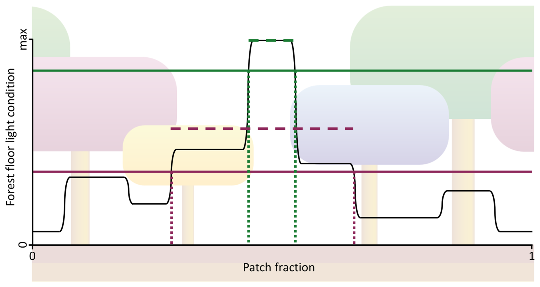
Figure 2 A visualisation of f_est,bm and f_est for new establishment using SEC (Fig. 1b). The visualisation includes the establishment of two PFTs: a shade-intolerant pioneer PFT (green lines) and a slow-growing, shade-tolerant PFT (purple lines). The range between dotted lines represents f_est, while the dashed lines indicate the mean PAR_est,i for the f_est ranges, and the solid lines show PAR_est,min. The value of f_est,bm is calculated as the ratio between the mean PAR_est,i to PAR_est,max described in Eq. (3).

To enable comparison, we introduced a perfect plasticity approximation (PPA) canopy scheme in LPJ-GUESS, based on the work of Strigul et al. (2008), Purves et al. (2008), and Fisher et al. (2010, 2018). In PPA, tree cohorts were organised according to height and arranged to perfectly fill the patch area. The tallest cohorts were assigned to the patch until their cumulative crown area equalled or exceeded the patch area. Once the patch was filled, an understory layer was created with the next tallest tree cohorts. If a cohort’s crown area could not fully fit within a single canopy layer, it was distributed across multiple layers (see blue cohort in Fig. 1c). Horizontal sections and light absorption within them were determined as per the SEC scheme, which resulted in the creation of five distinct vertical light profiles for the example in Fig. 1c. The herbaceous layer and light conditions for establishment were modelled similarly to the SEC scheme. In the PPA scheme (Strigul et al., 2008), each understory canopy layer receives the average light that penetrates through the layer above it. As a result, the position and height of cohorts within these layers become redundant, except for their allocation to specific layers. We modified this by assigning cohorts a specific horizontal position based on their height, allowing understory cohorts to intersect with the canopy layer above them if their height exceeded the bole height of the cohort above (see blue and green cohorts in Fig. 1c). This allowance for cohorts to occupy overlapping vertical space across canopy layers represents a key distinction from other implementations of the PPA framework (e.g. FATES; Fisher et al., 2015), in which cohorts from different canopy layers cannot intersect or interact. PPA shares similar challenges to LPJ when it comes to gap dynamics. If the total crown area of all cohorts exceeds the patch area, no gaps form within the canopy. To address this, some implementations of the PPA scheme introduced a gap fraction (η) that represents small gaps between trees within a cohort (Weng et al., 2015; Fisher et al., 2018). This feature allows more light to penetrate the canopy layers, improving light conditions for the understory and resulting in more realistic understory behaviour. However, our PPA representation did not incorporate this gap fraction tweak, so gaps only occurred when the total crown area of all cohorts was less than the patch area. Instead, we focused on structural features, such as tree and bole height, crown area, and cohort light interactions, as described earlier, as well as distinct forest floor light conditions for establishment. We considered these aspects to be more relevant to our study. Self-thinning in our PPA implementation was governed by both the general dynamic growth efficiency mortality and the over-crowding self-thinning mechanism, the latter as updated for SEC (Eq. 2). Additionally, the PPA method for organising the canopy horizontal structure led to dynamic promotion and demotion of cohorts between layers, depending on growth and mortality.

2.2 Model simulations

To validate the new canopy structure schemes, we performed model simulations using all four canopy schemes: LPJ, LPD, PPA, and SEC. For all schemes, we applied the standard LPJ-GUESS parametrisation without performing any additional scheme specific calibration. The model simulations were driven by the CRUNCEP global reanalysis climate dataset version 7 (Viovy, 2016), using a 30 year de-trended historical climatology from 1971 to 2000 to establish an equilibrium soil and vegetation condition over a 500 year spin-up period starting from bare ground and equal weighting between individuals of viable PFTs. During this spin-up phase, we introduced a stochastic, generic patch-destroying disturbance with a mean return interval of 100 years. After 500 years, a disturbance event reset the vegetation to bare ground, initiating a regrowth phase that lasted for an additional 1000 years under the same de-trended climate forcing. During this regrowth phase, no further disturbances were introduced, except in the LPD simulations, where disturbances continued with a 100 year mean return interval. Across all canopy structure schemes and for the full duration of the simulations, we used 100 replicate patches. The only exception was a sensitivity analysis in which the number of patches was varied. Fire was disabled for all simulations. The model was configured with 11 PFTs, as described in Table 1.

Table 1 Description of the plant functional types included in the study, highlighting the parameters that distinguish shade-tolerant from shade-intolerant PFTs.

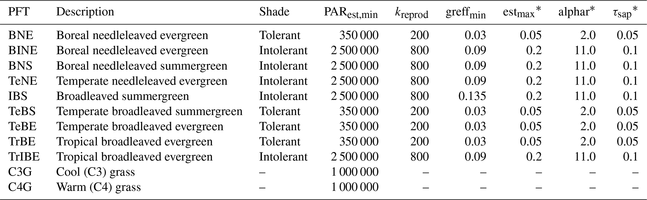
^∗ These parameters were not included in the model sensitivity analysis, as they are not directly affected by the new canopy schemes. They are: est_max, the maximum sapling establishment rate ($\mathrm{saplings}{\mathrm{m}}^{-\mathrm{2}}{\mathrm{yr}}^{-\mathrm{1}}$); alphar, a parameter describing the non-linearity of recruitment in relation to understory growing conditions for trees; and τ_sap, the annual sapwood turnover rate expressed as a fraction of sapwood C biomass.

2.3 Model evaluations

The model evaluation for stand structure and dynamics primarily relied on observations of aboveground woody biomass (AGB; $\mathrm{t}\mathrm{C}{\mathrm{ha}}^{-\mathrm{1}}{\mathrm{cm}}^{-\mathrm{1}}\mathrm{DBH}$), aboveground woody mortality (AWM; $\mathrm{t}\mathrm{C}{\mathrm{ha}}^{-\mathrm{1}}{\mathrm{yr}}^{-\mathrm{1}}{\mathrm{cm}}^{-\mathrm{1}}\mathrm{DBH}$), and aboveground woody productivity (AWP; $\mathrm{t}\mathrm{C}{\mathrm{ha}}^{-\mathrm{1}}{\mathrm{yr}}^{-\mathrm{1}}{\mathrm{cm}}^{-\mathrm{1}}\mathrm{DBH}$) collected from 25 large forest plots, as presented by Piponiot et al. (2022). To enable model comparison, the data are processed to $\mathrm{t}\mathrm{C}{\mathrm{ha}}^{-\mathrm{1}}{\mathrm{yr}}^{-\mathrm{1}}{\mathrm{cm}}^{-\mathrm{1}}\mathrm{DBH}$, i.e. AGB, AWP and AWM are provided across different diameter at breast height (DBH) size classes. For AGB, we standardised the observations into 16 DBH size classes: <1, <5, <10, <15, <20, <30, <40, <50, <60, <70, <80, <90, <100, <150, <200, and >200 cm. For AWM and AWP, the data were already standardised into 9 DBH size classes: <5, <10, <20, <30, <40, <50, <100, <200, and <500 cm. We excluded the smallest and largest size classes (<1 and >200 cm) for AGB as well as the largest size class (<500) for AWP and AWM.

The forest plots: SERC, MBW, and Palamnui were excluded from the analysis due to low growth biases detected during initial LPJ-GUESS simulations. Since this study aims to assess the impact of the new canopy structure representation rather than basic growth processes, these sites were not suitable for our tests. The San Lorenzo site was excluded because its coordinates, when converted to the climate-forcing resolution, corresponded to those of Barro Colorado Island. The Barro Colorado Island entry was updated to match the data provided by Legendre and Condit (2019). It is worth noting that some data from Piponiot et al. (2022) were gap-filled where discrepancies between observed and expected values occurred. Additionally, several study sites were subject to disturbance events of both natural and human origin. Table 2 offers a summary of all study sites and documented disturbances, although quantitative details remain limited for most events (Piponiot et al., 2022). In addition to the existing study sites, we incorporated AGB data from old-growth forests in five permanent monitoring plots within Białowieża National Park (Poland) by Brzeziecki et al. (2016) as well as data from 57 unmanaged sites across southern and central Finland by Peltoniemi and Mäkipää (2011). To ensure consistency across datasets, we interpolated the original DBH size classes from these sources to match the 16 DBH size classes used in the data compiled by Piponiot et al. (2022). This resulted in a total of 23 study sites distributed across five continents, representing three major forest climatic regions: 14 tropical, 5 temperate, and 4 boreal sites (Table 2). The sites are located in both old-growth and mature secondary forests.

Table 2 Overview of the study sites.

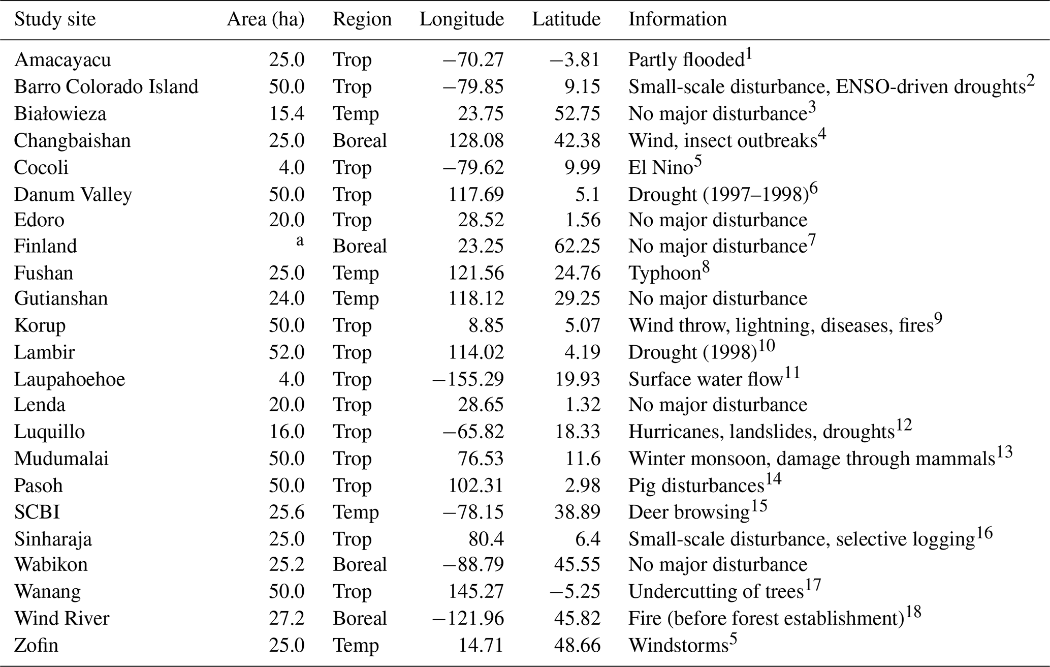
^a 57 unmanaged sites across southern and central Finland (Peltoniemi and Mäkipää, 2011).
References: ¹ López-Quintero et al., 2012, ² Koven et al., 2020, ³ Brzeziecki et al., 2020, ⁴ Zhang et al., 2023, ⁵ Piponiot et al., 2022, ⁶ Douglas, 2022, ⁷ Peltoniemi and Mäkipää, 2011 ⁸ Lin et al., 2011,⁹ Egbe et al., 2012, ¹⁰ Potts, 2003, ¹¹ Tweiten and Hotchkiss, 2009, ¹² Zimmerman et al., 2021, ¹³ Sukumar et al., 1999, ¹⁴ Peters, 2001, ¹⁵ Holm et al., 2013, ¹⁶ Alwis et al., 2016, ¹⁷ Vincent et al., 2015, ¹⁸ Shaw et al., 2004.

Our evaluation of the four canopy structure schemes focused on several key metrics. First, we assessed the accuracy of each scheme in replicating AGB, AWM, and AWP as a function of DBH size classes, comparing the results with observational data. Second, we examined the emergence of self-thinning patterns, mortality fluxes and rates, and the dynamics of functional coexistence within each scheme. Third, we analysed the re-establishment process following harvesting events across the different schemes. Fourth, we conducted two sensitivity tests: the first assessed how variations in wood density, establishment, and mortality rates affected functional coexistence, and the second investigated how the RMSE of AGB, AWM, and AWP, compared to observations, converged as the number of replicate patches increased.

The first two metrics were evaluated based on the basic model simulations across all 23 study sites. The analysis of the re-establishment process, as well as the sensitivity tests, was conducted using modifications to the basic simulations. For the third analysis (re-establishment processes following a harvesting event), the 1000 year regrowth phase was replaced with a harvesting event that occurs 80 years after the initial patch-destroying disturbance. Since re-establishment varies with harvest intensity, harvest events of the dominant cohorts were induced at different intensities: 0 % as a control, 10 %, 20 %, 30 %, 40 %, 50 %, 60 %, and 70 %. Post-harvest biomass in the recruiting layer was compared with the total biomass at 10, 30, and 60 years after the event. LPD was excluded from this analysis to ensure that patch-destroying disturbances did not affect the outcome. This analysis was carried out exclusively at the BCI site. The functional coexistence sensitivity tests involved pushing three key parameters in LPJ-GUESS to their extremes to examine the potential for coexistence between shade-tolerant and shade-intolerant PFTs over time. First, we tested the effect of wood density by doubling the wood density of shade-tolerant PFTs, thereby allowing shade-intolerant PFTs to grow taller faster than shade-tolerant PFTs. Second, we made the establishment of new saplings more uniform across all PFTs by increasing the background establishment factor (k_bgestab=0.1) and reducing the PFT-specific reproduction constant (k_reprod) by a factor of ten (Eq. 21 in Smith et al., 2001). These changes provided less dominant PFTs with a greater opportunity to establish. Finally, the growth efficiency mortality threshold (Eq. 31 in Smith et al., 2001), which determines the minimum growth efficiency (greff_min; $\mathrm{kg}\mathrm{C}{\mathrm{m}}^{-\mathrm{2}}\mathrm{leaf}{\mathrm{yr}}^{-\mathrm{1}}$) below which mortality occurs, was lowered for shade-intolerant PFTs to match that of shade-tolerant PFTs. Lastly, we evaluated the impact of the number of replicate patches on the RMSE of AGB, AWM, and AWP, relative to observations. For this test, all sites except BCI, BIA, and Finland were run again with varying numbers of replicate patches (1, 2, 5, 10, 15, 20, 30, 50, and 100) over the full simulation period.

2.4 Analysis framework

The scheme's performance was evaluated against observational data using the final simulation year. Both the model output and observational data were classified into the same DBH size classes: 16 classes for AGB and 9 classes for AWM and AWP. To ensure comparability across DBH distributions, both datasets were standardised to values per unit cm of DBH. For further analysis, AWM was normalised by AGB to provide a comparison of the aboveground woody mortality rates, rather than the flux itself. This approach was applied to both the observational and model data. All study sites were evaluated individually and as regional averages based on temperature. Białowieza and Finland were excluded from the analysis of AWM and AWP due to missing data. Independently of the observational data, the scheme's mortality fluxes were further analysed in order to understand the changing drivers of mortality. This analysis was performed for both LPJ and SEC, considering the total of above- and below-ground mortality instead of AWM. The fluxes included age mortality, self-thinning mortality, growth efficiency mortality, and other mortality. Self-thinning and growth efficiency mortality were grouped into a single class. The analysis did not consider DBH size classes, as fluxes were summed across all size classes and evaluated over the entire 1000 year regrowth period. Mortality rates were computed by dividing fluxes by the total biomass.

Self-thinning dynamics were assessed by examining the relationship between the number of trees (N; ha⁻¹) and the square root of their average quadratic mean diameter (Dg; cm), following Reineke (1933) and Bellassen et al. (2010), during the stand regrowth (years 10 to 100) and equilibrium (years 600 to 1000) phase

$$\begin{array}{}\text{(4)}& \ln \left(N\right)=c_{\mathrm{0}}+c_{\mathrm{1}}\ln \left(Dg\right)\end{array}$$

where c₀ is the intercept and c₁ is the slope.

To analyse functional coexistence, we examined biomass over the entire time series, averaging across all sites, and with PFTs categorised into three groups: shade-tolerant, shade-intolerant, and grass. This grouping allowed for a meaningful comparison of study sites with varying PFT compositions. The re-establishment test defined the recruitment layer as cohorts with a DBH smaller than 15 cm. The biomass of the recruitment layer was divided by total biomass to determine the fraction of biomass in the recruitment layer. The impact of varying simulated patch numbers was evaluated by computing the normalised distribution of AGB, AWM, and AWP across DBH classes, and then calculating the RMSE relative to observations. This test did not focus on the absolute values but on the speed at which different canopy schemes converge to estimate the optimal number of patches required for each scheme.

3 Results

3.1 Stand structure and dynamics evaluation

When comparing the biomass distribution across size classes for the final simulation year with the combined observational data from all biomes, LPJ generally captured the biomass distributions of large size classes in temperate and boreal regions (Fig. 3a–c), but tended to underestimate biomass in smaller size classes in temperate and tropical regions. In tropical sites, the overall overestimation was primarily driven by excessive biomass in large size classes. Conversely, LPD exhibited a notable leftward shift in the distribution towards smaller size classes. This shift was a result of the recurring patch-destroying disturbances that reset the patches to bare ground, increasing the occurrence of small size class trees. Consequently, LPD significantly underestimated total biomass compared to the observations. Similar to LPD, PPA and SEC simulated a greater biomass fraction in smaller trees. Their more detailed canopy structure allowed them to better align overall biomass with the observations, particularly at the tropical study sites. LPJ and SEC had the highest total mean biomass across the sites of the schemes with 196 and 161 t C ha⁻¹, respectively. PPA had a total mean biomass of 133 t C ha⁻¹ and LPD the lowest with 113 t C ha⁻¹. The reason for such low overall biomass for LPD (Fig. 3a–c) lay again in the recurring patch-destroying disturbances. The biases in woody biomass-size distributions were ultimately caused by the interaction between growth and mortality rates. When comparing the simulated growth rates to observations over all sites, it became evident that all model versions underestimated the AWP flux (Fig. 3d–f). This general underestimation was likely a result of other model biases not related to the canopy schemes, e.g. GPP or allocation of C to wood, which was beyond the scope of this work to address. What is more important for this study was the shape of growth and mortality rates across DBH size classes, as compared to the observations. In this regard, LPJ significantly underestimated the AWP flux across all size classes, except for the largest trees. Conversely, LPD exhibited a bias towards smaller size classes, consistent with its woody biomass bias. PPA and SEC simulated an AWP flux distribution across size classes that more closely aligned with observations, although the absolute values remained lower, with PPA being closest to observed values. When analysing individual regions, all canopy schemes tended to underestimate the AWP flux in tropical and temperate study sites (Fig. 3d–f). In boreal study sites, AWP flux for smaller size classes (up to <30) was overestimated by all canopy schemes except for LPJ, whereas larger size classes were consistently underestimated. Overall, larger tree cohorts in LPJ accounted for an overly large share of the AWP flux, whereas in LPD smaller tree cohorts contributed disproportionately to the AWP flux. In contrast, PPA and SEC more successfully capture the broad patterns of AWP flux distribution. Similar to the fluxes of AGB and AWP, LPJ tended to underestimate the AWM fluxes for smaller size classes and could not capture the AWM flux pattern in any of the tropical, temperate, and boreal study regions (Fig. 3g–i). LPD, PPA, and SEC had the same issue in the boreal study sites. However, they exhibited a better agreement with observed patterns in tropical and temperate regions.

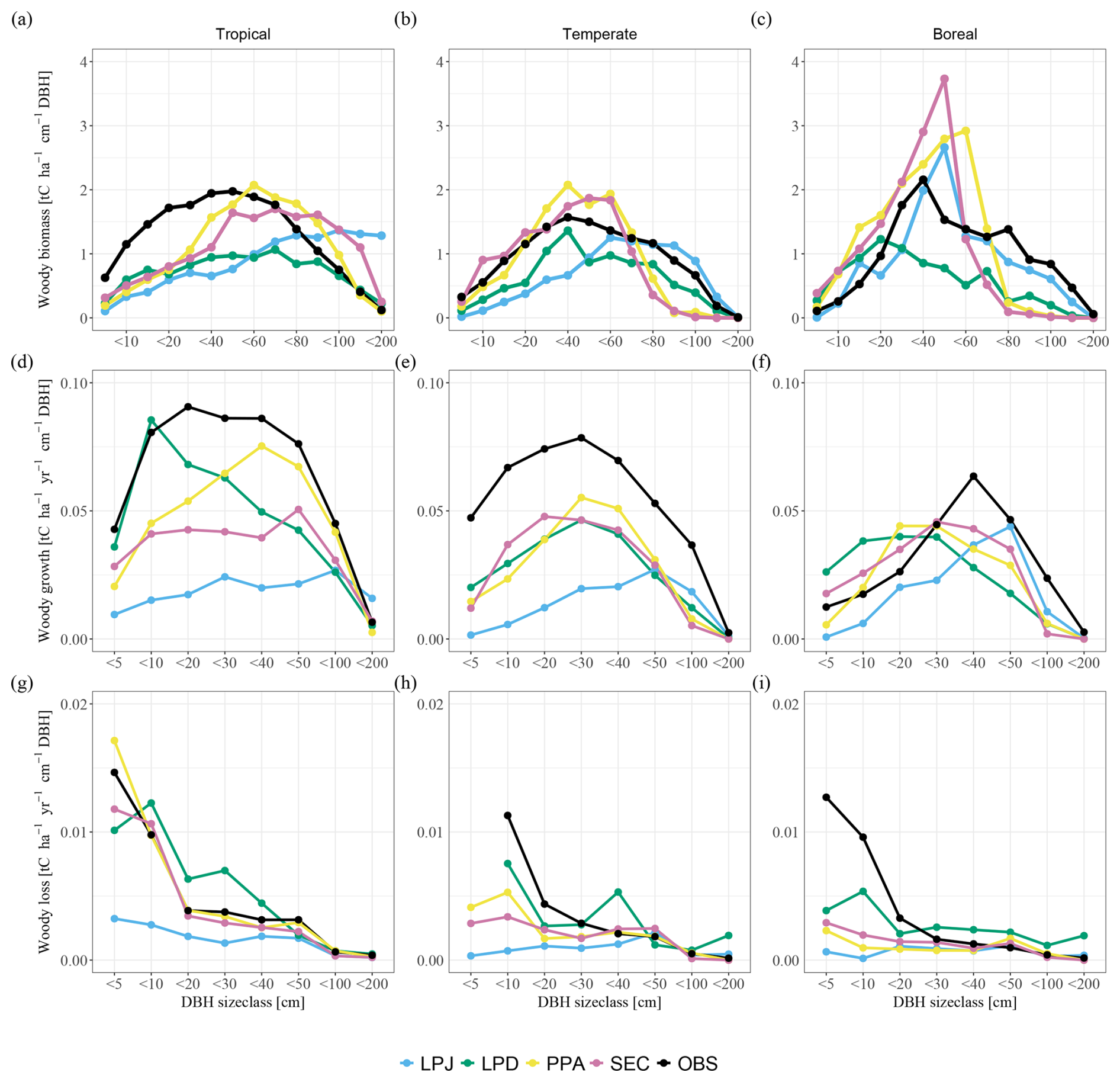
Figure 3 Comparisons of woody biomass (a–c), aboveground woody productivity (d–f), and aboveground woody mortality (g–i) across DBH size classes, averaged over biomes. Columns indicate the biomes (from left to right): tropical, temperate, and boreal.

All canopy schemes exhibited emergent self-thinning behaviour when averaged across all sites during the initial regrowth phase, the first 100 years of stand development (coloured circles in Fig. 4). In the LPJ scheme, tree numbers declined clearly as mean stem diameter increased throughout regrowth. After about 30 years, the mean number of cohorts per patch decreased significantly, leaving only a few cohorts to shape the stand’s structure (Fig. 4a, inset graph). While LPD initially followed a similar trend to LPJ, disturbances that reset patches caused the cohort numbers to stabilise, and stem diameter growth levelled off at a lower value than in LPJ. This stabilisation was a result of patches frequently resetting to bare ground, effectively resetting the patch age to zero. In contrast, both PPA and SEC started with a higher density of smaller-diameter trees, because forest floor light conditions remained favourable for establishment longer than in LPJ and LPD. As a result, both schemes exhibited a clear decline in tree numbers due to self-thinning as stem diameter increased during the regrowth phase. Once the stand reached around 1100 (650) trees with a mean stem diameter of approximately 18 (22) cm, the SEC (PPA) structure stabilised due to self-thinning and mortality factors linked to competition, which created space for new trees to establish.

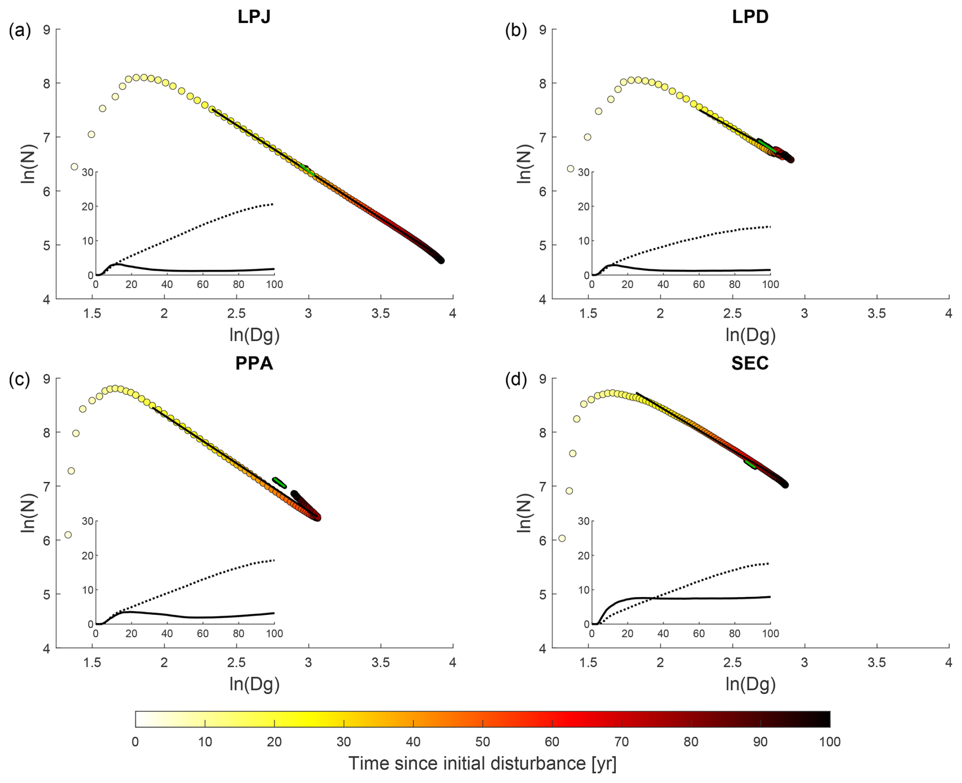
Figure 4 Tree size and density dynamics during stand regrowth (years 0 to 100) and equilibrium (years 600 to 1000) phases. N (ha⁻¹) represents the average number of trees across all sites, while Dg (cm) is the average quadratic mean diameter. The marker fill colours indicate the time elapsed since the initial disturbance that initiated the regrowth phase. Lines (black – regrowth years 20 to 90, green – equilibrium phase) represent the Reineke slope (c₁), while the black dots represent data from the equilibrium phase. The inset graph shows on the y axis the average number of cohorts per patch (solid line) and AGB (dotted line; kg C m⁻²) across all sites during the regrowth phase years (x axis).

When comparing mortality fluxes and rates during the regrowth phase for LPJ and SEC (Fig. 5), both schemes displayed similar patterns. A strong peak in competition-based mortality occurred early in the regrowth phase due to self-thinning. As the stand aged and approached equilibrium, the dominant mortality mechanism shifted to age- and size-related competition (Fig. 5). The increasing competition from uneven-size cohorts led to higher mortality, as the growth efficiency of individual trees decreased due to shading from larger cohorts. During the equilibrium phase, LPJ had the fewest trees on average (N=600), but with the largest mean DBH (Dg=20 cm). LPD and PPA reached similar equilibrium states, with tree densities of N=900 and N=1200, and corresponding DBH values of Dg=15.5 and 16.5 cm, respectively. SEC exhibited the highest tree density (N=1600) but the smallest DBH (14 cm).

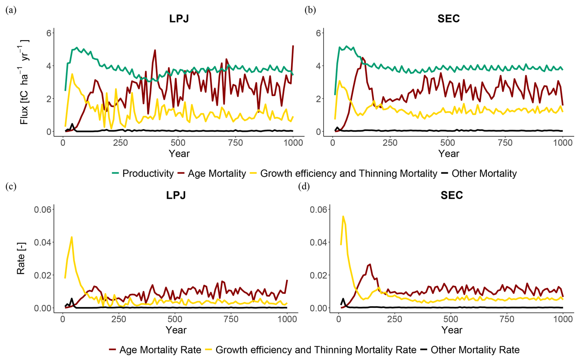
Figure 5 Mortality fluxes (top) and rates (bottom) at BCI. Productivity refers to woody biomass growth, while mortality fluxes indicate the loss of woody biomass from the stand to the litter pool.

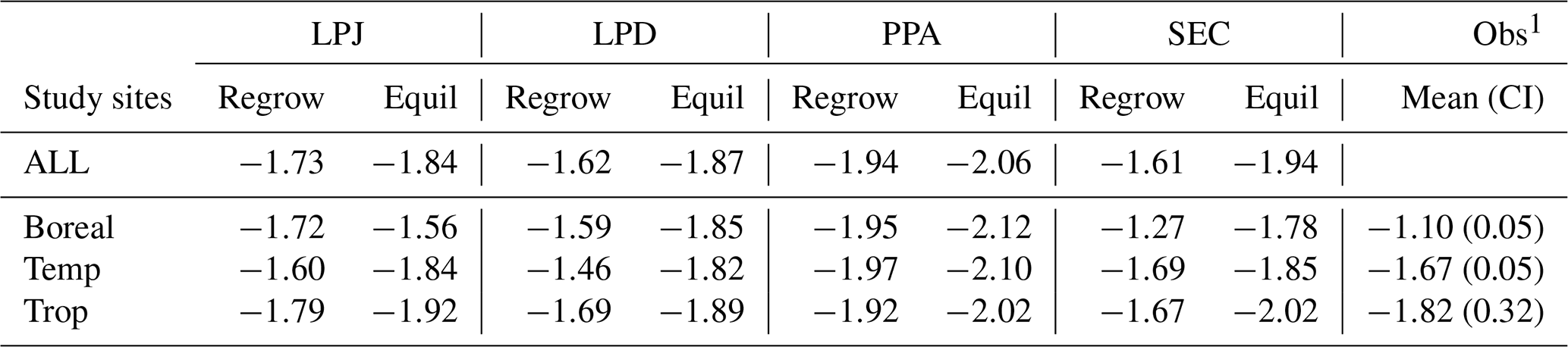
Analysing the Reineke self-thinning slopes (c₁) across all sites (Fig. 4) for the different canopy schemes revealed that PPA had the steepest overall slope (Table 3) during regrowth, which meant that its mean DBH increased the least as tree density decreased. SEC, LPD, and LPJ showed significant variation across climatic regions, whereas PPA did not. Tropical sites generally exhibited the steepest slopes, except for PPA, which had the shallowest slope in this region. In temperate zones, LPJ and SEC showed similar slopes, while LPD had the shallowest slope. In boreal regions, SEC displayed the shallowest self-thinning slope, leading to the fastest mean DBH increase as tree density decreased. Overall, the equilibrium phase tended to have a steeper slope than the regrowth phase as tree density fluctuated. PPA had the steepest slope, with SEC showing the second steepest. LPJ had the shallowest slope, particularly in the boreal region. LPJ and SEC showed a distinct increase in slope with warmer climates during the equilibrium phase.

Table 3 Average Reineke (1933) slope (c₁) for the regrowth (Regrow – years 20 to 90) and equilibrium (Equil – years 600 to 1000) phases across all sites and within specific climatic regions. Observed means and confidence intervals (CI) for the climatic regions, as reported by Yu et al. (2024).

¹ Yu et al. (2024).

3.2 Functional coexistence

LPJ simulated initial coexistence of PFTs following the patch-destroying disturbance event. However, after approximately 150 years, shade-tolerant PFTs began to outcompete shade-intolerant PFTs, ultimately dominating the stands within 200 to 350 years (Fig. 6a–c). During this period, the biomass of shade-intolerant PFTs decreased to zero, while shade-tolerant PFTs maintained relatively stable biomass levels for the remainder of the simulation. LPD produced divergent results (Fig. 6d–f); shade-intolerant PFTs maintained a stable biomass throughout the simulation, while shade-tolerant PFTs still dominated the ecosystem on average across all sites. This dominance was more pronounced in productive areas, particularly in tropical sites, whereas in boreal regions, shade-tolerant dominance was distinct. PPA and SEC showed a much higher initial biomass peak for shade-intolerant PFTs compared to LPJ and LPD. In PPA (Fig. 6g–i), shade-intolerant PFTs initially dominated in all biomes and maintained this dominance in tropical regions throughout the simulation. In temperate regions, their abundance declined, as seen in LPJ. In boreal regions, both shade-tolerant and shade-intolerant PFTs persisted at high levels, consistent with patterns seen in LPD. In SEC (Fig. 6j–l), temperate sites generally followed the PPA trend, while boreal sites showed a slight dominance of shade-tolerant PFTs, but only when the stands became very old. In tropical regions, shade-tolerant PFTs became dominant over time, but unlike in LPJ or PPA, a stable underlayer of shade-intolerant PFTs persisted throughout the simulation period. Generally, there was greater variability across individual sites, and some exhibited high levels of coexistence between shade-tolerant and shade-intolerant PFTs.

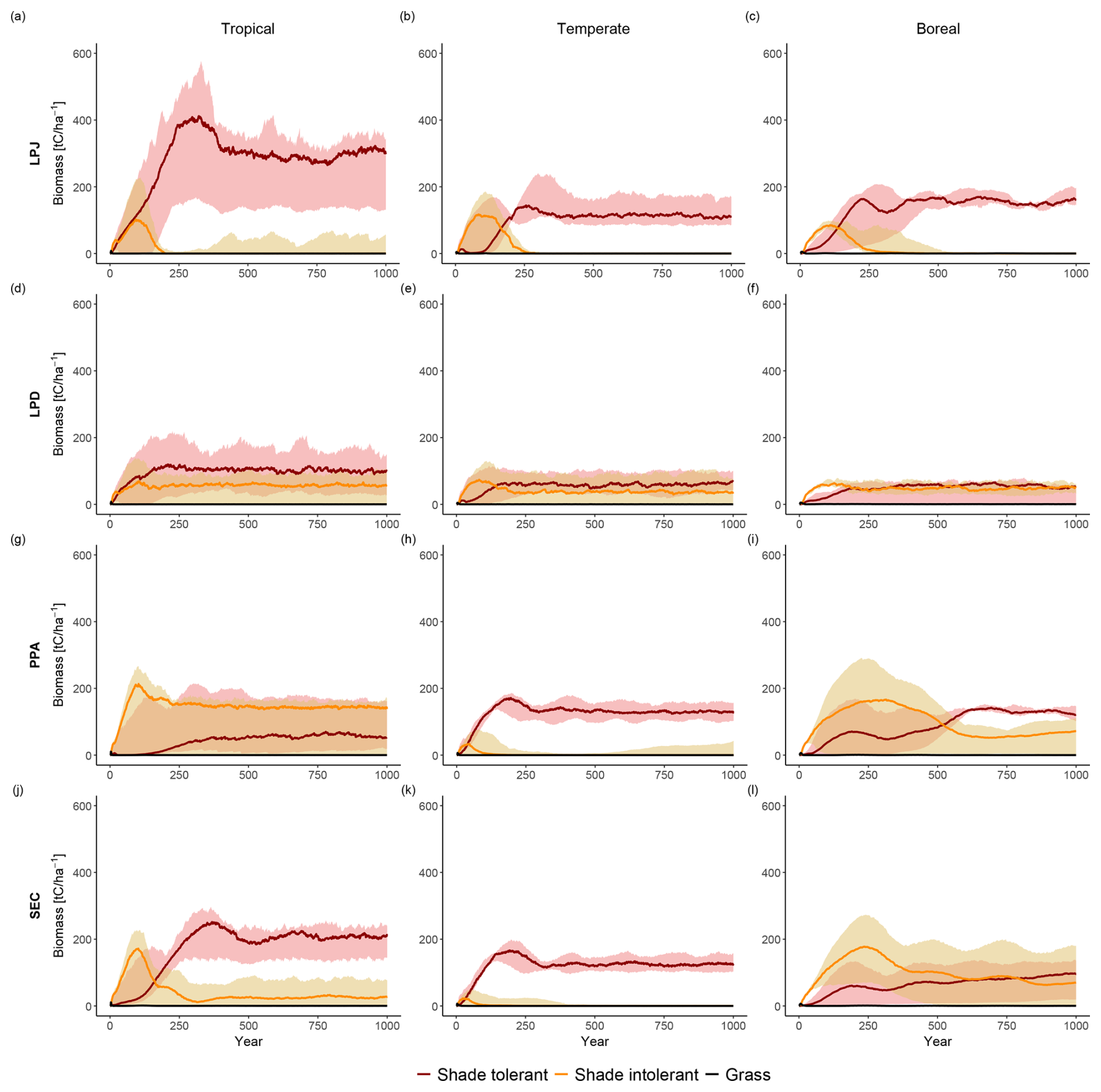
Figure 6 Comparison of functional coexistence among grouped plant functional types (shade-tolerant trees, shade-intolerant trees, and grasses), with results expressed as biome-level averages across all study sites. Rows correspond to the canopy structure schemes (from top to bottom): LPJ, LPD, PPA, and SEC. Columns indicate biomes (from left to right): tropical, temperate, and boreal.

All schemes initially displayed a typical pattern of forest dynamics: shade-intolerant PFTs established first following a disturbance event, and over time, were gradually replaced by shade-tolerant PFTs. LPD and PPA maintained high coexistence between these PFTs over time, whereas LPJ and SEC showed less coexistence on average. When analysing the sensitivity of coexistence to changes in wood density, establishment, and mortality (Fig. 7), LPJ initially showed a strong response to doubling the wood density of shade-tolerant PFTs. Despite this, shade-tolerant PFTs eventually dominated. Changes to establishment and mortality had minimal effects on LPJ’s coexistence patterns. Changes to establishment rates had little impact on LPD and PPA, which already exhibited coexistence. However, alterations to wood density and mortality caused shade-intolerant PFTs to dominate, particularly with changes in wood density. For the SEC scheme, increasing wood density alone promoted higher coexistence initially, but shade-tolerant PFTs still dominated over time. When increased wood density was combined with adjustments to mortality and establishment, SEC was capable of simulating sustained coexistence throughout the simulation (Fig. 7, bottom row).

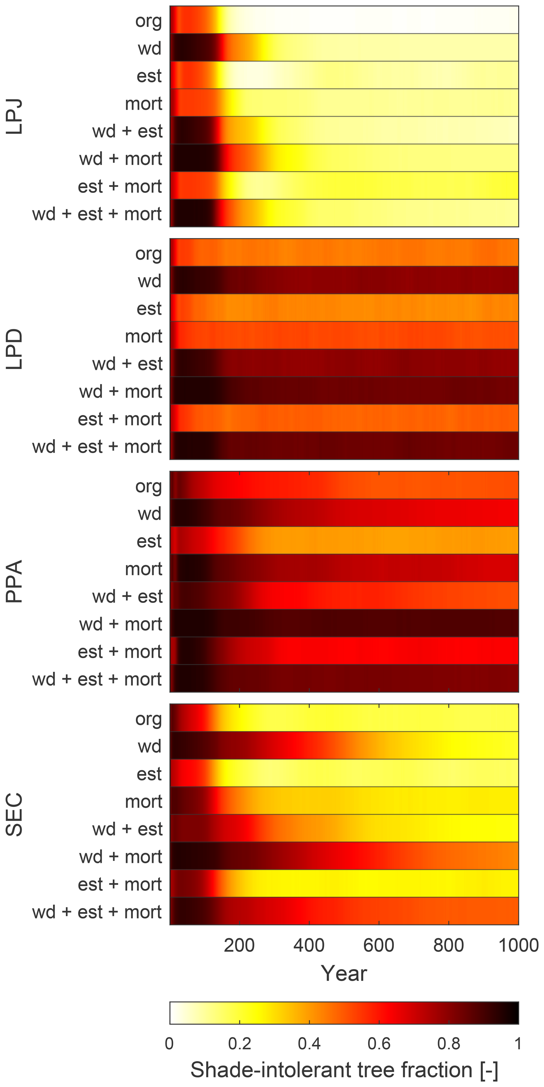
Figure 7 Fraction of coexisting shade-tolerant and intolerant PFTs when wood density (wd), establishment rate (est), and mortality rate (mort) have been changed. org – default implementation.

3.3 Re-establishment

LPJ was unable to simulate a persistent recruitment layer at any level of harvesting at BCI (Fig. 8). In contrast, PPA was able to simulate the formation of a recruitment layer at a 20 % harvest level, though for it to persist beyond 10 years, harvest levels above 40 % were required. No harvest level allowed the recruitment layer to endure for 60 years. SEC successfully maintained a recruitment layer beyond 60 years, even at a 20 % harvest level, with higher harvest levels resulting in an increased fraction of stand biomass allocated to the recruitment layer.

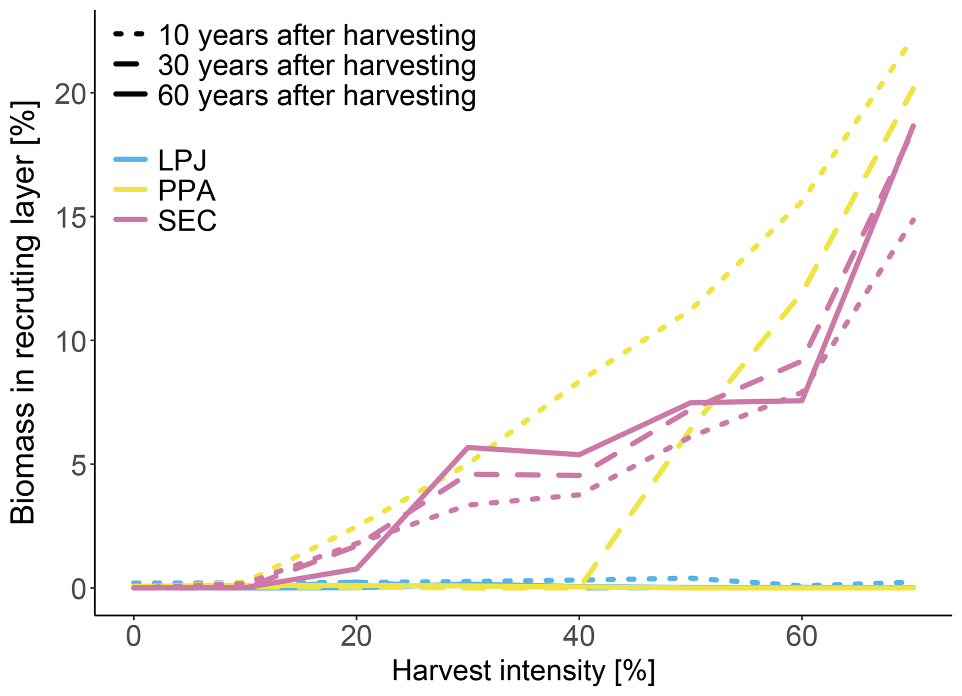
Figure 8 Re-establishment 10, 30 and 60 years after a harvest event, with a harvest strength of 0 %–70 % at BCI. Biomass in the recruiting layer is shown as fraction of total biomass.

3.4 Influence of number of patches

LPJ exhibited the highest RMSE value across all number of simulated patches when it comes to biomass, productivity, and mortality (Fig. 9). However, like PPA and SEC, it converged quickly for biomass and productivity with relatively few patches. To achieve an RMSE within 50 % of the final biomass observed at 100 patches, LPJ and SEC only required 10 patches, whereas PPA needed 15 and LPD 20 patches. For productivity, LPJ, PPA, and SEC required 15 patches and LPD 20. In terms of mortality, LPJ and PPA converged more slowly than LPD and SEC, with SEC and LPD reaching convergence the fastest falling below the 50 % RMSE threshold with 20 patches, while LPJ and PPA required 30 patches. Considering the different convergence rates of the canopy schemes, it was also important to evaluate their runtimes for the simulated sites in this study. Since LPD is the standard scheme in LPJ-GUESS, the different runtimes were compared against it. On average, LPJ required 1.14 times the runtime of LPD, PPA required 1.54 times, and SEC required 2.26 times.

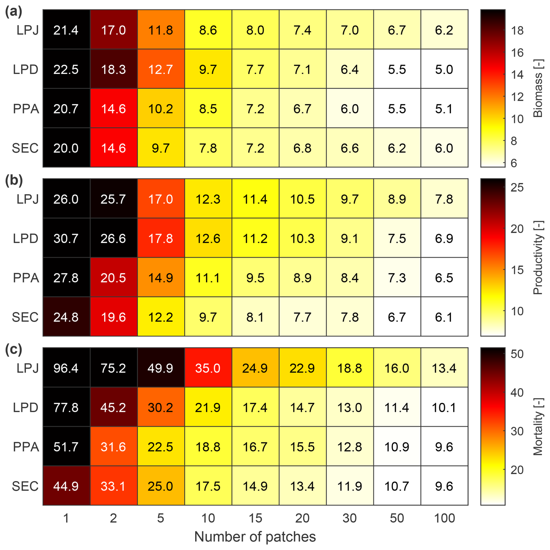
Figure 9 The impact of varying simulated patch numbers on RMSE for woody biomass (a), productivity (b), and mortality (c) against observations across all sites, excluding BCI and Finland. AGB, AWM, and AWP are normalised across DBH classes.

4 Discussion

The key reasons for incorporating the more detailed stand structure capability SEC into LPJ-GUESS were: (a) to enable closer alignment with observational data, thereby providing better constraints on the processes governing growth and mortality, and (b) to enhance the model's capability to represent critical forest features, including tree functional coexistence and the impacts of small-scale disturbances, such as mortality or self-thinning, on stand dynamics. In this respect, the development has proven largely successful.

Simulating stand biomass-size distributions with the more detailed canopy schemes revealed an improvement compared to LPJ, but no improvement compared to LPD. This outcome was expected, as LPJ-GUESS has been calibrated and developed over decades using LPD. Size distributions are fundamental relationships that have shaped the evolution of the model over several years. They are heavily influenced by growth and mortality rates throughout stand development and can also be significantly affected by individual disturbance events. The absence of horizontal spatial structures within a patch favoured the dominance of the tallest tree cohort as well as the lack of patch-destroying disturbances that would otherwise reset the patch to bare ground. For LPJ, this led to an extreme shift of AWB and AWP towards larger size classes, resulting in a representation that is far from reality. LPD, as well as the new canopy schemes, counteracts this effect using different approaches. LPD was developed with the assumption that periodic patch resetting is necessary to achieve a good size distribution. Figures 4, 6, and 7 clearly illustrate that the resetting of patches, caused by patch-destroying disturbances with a mean return interval of 100 years, caused LPD to closely resemble an average state of LPJ at a stand age of around 100 years. In contrast, both PPA and SEC could achieve a size distribution closer to observations without relying on such disturbances. PPA accomplished this by accounting for each cohort's crown area when distributing light interception between cohorts, a factor that allows more cohorts to occupy the upper canopy; an effect which is absent in LPJ and LPD. However, when the total crown area exceeded the patch area in PPA, canopy gaps could not form by construction, substantially constraining the establishment of smaller, shade-intolerant PFT cohorts. In contrast, SEC represented a mixture of size classes and allows for the formation of canopy gaps independent of the total amount of crown area, thereby explicitly overcoming this structural constraint of PPA and promoting the establishment of various PFTs. Since light is a critical resource for photosynthesis and its availability often limits plant growth in lower layers of forest ecosystems, gap formation can significantly boost photosynthetic activity, especially in newly established plants (Chazdon et al., 1996), resulting in a more accurate representation of size distributions. By enabling spatially explicit canopy gaps, SEC produces more realistic understory light environments and competitive interactions, opening new opportunities to investigate regeneration niches, gap dynamics, and demographic coexistence within a different conceptual framework. While SEC itself was not included in the demographic vegetation model intercomparison of Eckes-Shephard et al. (2025), the study demonstrated that many PPA-based models delay thinning until the light environment is fully saturated, whereas gap-based approaches induce mortality in suppressed cohorts as soon as canopy closure reduces understory light. This highlights the type of dynamics that SEC captures without requiring explicit individuals, thereby expanding methodological options for bridging individual-based and cohort-based forest modelling frameworks.

Still, a reparameterisation of LPJ-GUESS using the new canopy structure schemes is necessary to further enhance the model's ability to align with observational data at particular sites or in global application. This is especially important for the representation of woody growth and woody mortality rates, which influence AGB. A slight shift towards larger size classes, similar to LPJ, was still present for PPA and SEC schemes. Crucially, however, the general agreement between observations and model was not degraded using the new canopy schemes, demonstrating that the more detailed structure did not lead to a fundamental misrepresentation of the size distribution of the forest. Supporting this, all schemes produced Reineke slope values within the ranges reported in the literature: Pretzsch and Biber (2005) reports a range from −1.42 to −1.79, and Trifković et al. (2023) from −1.19 to $-\mathrm{2.00}.$ Notably, the mean Reineke slope for the SEC scheme was −1.61, closely matches the original global estimate by Reineke (1933) of $-\mathrm{1.605}.$ LPJ and SEC also showed an increase in slope with warmer climate regions, consistent with the findings of Yu et al. (2024). All schemes exhibited a slope that was too steep at equilibrium in boreal and temperate regions, whereas in tropical regions, all schemes fell within the confidence interval of the observations reported by Yu et al. (2024).

Beyond stand biomass-size distributions, species coexistence also plays a crucial role in many forests and thus it is important to be able to explore its impacts in VDMs. Coexistence was more realistically represented in the new SEC canopy scheme. Natural disturbances create openings in the forest canopy, allowing light to reach the forest floor and give opportunities for various species to establish and co-exist, enhancing species diversity (Viljur et al., 2022). Following a gap creating disturbance, fast-growing, light-demanding species initially colonise the area. Over time, these species are replaced by slower-growing, shade-tolerant species as the canopy closes and light availability decreases (Wright et al., 2010). While shade-tolerant species with survival-focused traits tend to dominate in stable, low-light environments, shade-intolerant species grow quickly, are more prone to death and can be found in canopy gaps or disturbed areas where light is abundant (Wright et al., 2010). In order to represent species coexistence a VDM should be able to capture these dynamic processes. Also, it should be able to account for both the initial colonisation by light-demanding species and the subsequent succession to shade-tolerant species, reflecting the ecological balance driven by disturbances and canopy dynamics. Initially, LPJ demonstrated a good representation of functional coexistence (Figs. 6a and 7), however after around 200 years, even when three key growth and survival parameters were adjusted to favour shade-intolerant PFTs (Fig. 7), shade-tolerant PFTs began to dominate, leading to the near disappearance of shade-intolerant PFTs. A higher reproduction C flux from the more abundant shade-tolerant PFTs even reinforced this dominance, further securing their strength in the ecosystem caused by a higher establishment rate. As this dominance persisted even when adjusting parameters and forest structure conditions more favourable for shade-intolerant species, we concluded that a long-term coexistence with shade-tolerant species was not possible in an LPJ approach. Again, the core issue lies in this version’s lack of horizontal spatial structure within the canopy. As a result, all cohorts end up shading one another, creating an environment where shade-tolerant PFTs thrive while shade-intolerant species are disadvantaged as soon as their canopy intersects with others. This structural limitation leads to the competitive exclusion of shade-intolerant PFTs. LPD maintained a functional coexistence throughout the simulation (Figs. 6b and 7), however, these reliable results depended on the recurring patch-destroying disturbances, which reduce the average patch age of LPD to about 100 years, maintaining conditions similar to the LPJ state at year 100. As a result, the standard representation of canopy structure in LPJ-GUESS can simulate coexistence in young, disturbed ecosystems but struggles to represent coexistence in old-growth, undisturbed forests, where allogenic (external) disturbances are absent. Whilst patch-destroying disturbance rate in LPD can be parameterised to integrate over mortality at a range of scales, it can not take advantage of the emerging observational constraints on mortality at different scales (e.g. Esquivel-Muelbert et al., 2020; Senf and Seidl, 2021).

The new canopy schemes generate reliable results resulting from a more realistic representation of forest horizontal structure. PPA's forest composition is characterised by a high proportion of shade-intolerant PFTs (Figs. 6c and 7), as the tallest trees are rarely shaded unless a second canopy layer forms, which occurs when the total crown area exceeds the patch area. In this case, the upper canopy is partially shaded by the second layer if the tree heights surpass the bole height of the upper-layer trees. Since shade-intolerant PFTs grow taller more rapidly than shade-tolerant PFTs, they consistently occupy the upper canopy layer with minimal disturbance. Similar to LPJ, this dominance is reinforced by the higher reproduction C flux for establishment by the dominant PFTs. The implementation of the new SEC canopy structure scheme leads to a more nuanced coexistence through varying light conditions throughout the patch (Figs. 6d and 7). We demonstrate that, in the absence of a patch-destroying disturbance, variation in the level of functional coexistence is structurally possible by only modifying three key parameters (Fig. 7). The SEC scheme permits openings in the forest canopy, allowing light to reach the forest floor, and giving opportunities for various PFTs to establish and co-exist. This capability of representing forest gaps enhances LPJ-GUESS's capability to represent species diversity. Following a gap-creating event, fast-growing, shade-intolerant PFTs initially colonise the area. Over time, these PFTs are replaced by slower-growing, shade-tolerant PFTs as the canopy closes and light availability decreases. As evident in Fig. 7, the SEC canopy scheme has the capability to be parametrised to have increased or decreased coexistence. Importantly, the SEC scheme can also make better use of the emerging observational constraints than LPJ or LPD.

The improvement of LPJ-GUESS by implementing more realistic canopy structure representations allows the new schemes to display a more realistic establishment after harvesting. Previous empirical studies have demonstrated the necessity of harvesting in order to promote establishment. For example, tropical forest gaps as small as 50 m² have been shown to significantly affect species composition, while larger gaps of 100–300 m² are shown to actively promote new establishment of a broader range of species (Denslow, 1987). Generally, tropical forests benefit from gaps ranging from 100–400 m², created by removing around 10 %–20 % of canopy trees (Ghazoul et al., 2015). In mixed-species temperate forest successful regeneration is found when applying harvesting practices of removing 15 %–35 % of live trees, simulating natural disturbances (Puettmann et al., 2012). Temperate forests benefit from smaller gaps compared to tropical forests ranging from 10–150 m², created by removing around 15 %–30 % of canopy trees (Larson and Churchill, 2012). For boreal forests, reducing the canopy density by 20 %–50 %, with gaps typically ranging from 50 to 200 m² has been found to generate sufficient light conditions to promote the establishment of shade-intolerant species (Thorpe and Thomas, 2007). With the standard LPJ-GUESS canopy structure scheme (LPJ), the absence of horizontal spatial structure within the canopy prevents the formation of a recruitment layer (Fig. 8). For a new cohort of any PFT to establish the average LAI must be low enough to create favourable light conditions on the forest floor. But even a 70 % reduction in LAI appears insufficient (Fig. 8). In contrast, both PPA and SEC canopy schemes generate a recruitment layer with harvest intensities as low as 20 %, aligning more closely with the studies discussed earlier. Within 10 years of harvesting, PPA shows the fastest-growing recruitment layer (dash-dotted lines, Fig. 8). However, over time, PPA cannot sustain this recruitment layer. After 30 years, a harvest rate of 50 % is required to maintain it, and by year 60, no recruitment layer remains. As tree crown area started to fill the patch area in PPA, the recruitment layer is eventually shaded out once the initial cohorts had grown so that their combined crown area matches the patch area again. At the BCI site, this occurs with harvest intensities below 50 % within 30 years, and by 60 years the recruitment layer disappears. In SEC, while the recruitment layer develops more slowly compared to PPA, it remained stable over time. As the canopy gaps have distinct locations, the initial cohorts must grow large enough to fill these gaps before the recruitment layer could reach sufficient height to compete for light. The proportion of biomass in the recruitment layer remains relatively constant over time for all harvest intensities that allowed a recruitment layer to be established. This stability is due to the prolonged existence of the canopy gaps, which enable the recruitment layer to grow and compete with the established cohorts.

Finally, the new canopy schemes have not degraded the technical performance. To capture the distribution within a landscape, LPJ-GUESS simulates a suite of patches to represent vegetation stands with different disturbance histories and developmental stages (Smith et al., 2001, 2014). The number of patches required for the standard canopy scheme LPD varies depending on the research question. For studies focused on average global fluxes and pools, approximately 15 patches may suffice. However, for questions that target site- to regional-scale dynamics, a larger number of patches is necessary to account for the variability caused by the recurring, patch-destroying disturbances. As visible in Fig. 9, LPD required a substantial number of patches to achieve convergence when calculating the RMSE for biomass, productivity, and mortality. When the RMSE has converged, the addition of more patches would not improve the simulated result. Increased model complexity often leads to longer run times. The SEC scheme, which represents a canopy structure with greater complexity than LPD, demanded more than twice the computational resources. Fortunately, SEC exhibited a faster convergence in RMSE with fewer patches, making it feasible to operate with a reduced number of patches depending on the overarching stand-replacement disturbance regime of the area. This capability allows for reliable results while decreasing model run duration and lowering memory usage.

One limitation shared by all of the canopy schemes is that tree individuals within a cohort do not interact with one another in terms of shading. They are positioned in perfect alignment, with no overlap in their crowns. As a result, the total crown area (CA_i) for each cohort increases linearly as the identical trees in the cohort grow. Additionally, none of the schemes account for the angle of the sun, assuming instead that all solar radiation comes directly from the zenith. Therefore, the PAR used in this study is adjusted for the solar zenith angle. Under this assumption, LPJ and LPD are unaffected with respect to gap dynamics, as neither scheme represents canopy gaps explicitly, whereas in both PPA and SEC the solar angle would influence the amount of direct light reaching the forest floor through canopy gaps, with lower solar elevations reducing understory direct light availability (e.g. Sato et al., 2007). This effect is not represented in the present study but will be examined in future work. In SEC, gaps are spatially explicit, while in PPA gap availability is constrained once total crown area exceeds the patch area. It is also worth noting that individual calibrations for each canopy scheme had not been performed prior to this study. Since LPD is the standard canopy scheme for LPJ-GUESS, it has undergone extensive calibration over the years.

5 Conclusions and outlook

The development of the new canopy structure scheme, SEC, marks a significant advancement in the representation of forest patch horizontal heterogeneity within LPJ-GUESS and provides an important alternative to the growing dominance of PPA-based frameworks. This innovative scheme is capable of properly representing the size structure of biomass, productivity, and mortality across a set of sites in boreal, temperate, and tropical regions. It also allows for the representation of functional coexistence without the influence of large-scale disturbances and captures the interplay of forest gap dynamics with the establishment of a recruitment layer, an aspect which, using the standard canopy structure representation in LPJ-GUESS, was previously not possible. Moreover, in contrast to PPA, SEC avoids the instantaneous promotion and demotion of cohorts between canopy layers that occur when the total crown area exceeds the patch area, thereby providing a more gradual and ecologically consistent representation of canopy reorganization. It is also anticipated that incorporating this more sophisticated canopy structure scheme will reduce biases related to stand structure and composition by more accurately representing the key processes driving vegetation and ecosystem dynamics. The presented results give confidence that the SEC canopy scheme can enhance LPJ-GUESS's capability to simulate forest demography more faithfully, especially after proper parametrisation. This advancement opens up new possibilities for improving the capability of simulating various processes, such as fire and tree mortality, in a more sophisticated manner. Ultimately, this will lead to an improved estimation of the demographic processes that drive temporal shifts in plant populations, community composition, carbon, nutrient, and water fluxes, as well as overall structure within terrestrial ecosystems, which are key processes for understanding the influence of a changing climate on our ecosystems.