Curlew 1.0: Spatio-temporal implicit geological modelling with neural fields in python

We present curlew, an open-source python package for structural geological modelling using neural fields. This modelling framework incorporates various local constraints (value, gradient, tangent and (in)equalities) and tailored global loss functions to ensure data-consistent and geologically realistic predictions. Random Fourier Feature (RFF) encodings are used to improve model convergence and facilitate stochastic uncertainty quantification, while simultaneously improving the model's ability to learn naturally periodic features such as folds. These advances are integrated into a software framework that allows incremental construction of complex geological models through temporally-linked neural fields, each representing a specific deposition, intrusion or faulting event. Significantly, this framework allows semi-supervised learning to integrate diverse unlabelled datasets (e.g., geochemistry, petrophysics), reducing interpretation bias and potentially improving model robustness. We describe and demonstrate these various capabilities using synthetic examples and real data from a faulted stratigraphic digital outcrop model from Newcastle, Australia.

1 Introduction

Three-dimensional (3D) structural geological models (SGMs) integrate disparate geological and geophysical data to make predictions about the subsurface distribution of rock types (Wellmann and Caumon, 2018). The results can be used to inform our understanding of large-scale processes, like plate tectonics, geomorphology and hydrogeology. For example, SGMs can provide crucial constraints on construction works (such as tunnelling), guide minerals explorationists and mine operators that supply society with metals, and are fundamental to successful groundwater modelling and management, geothermal energy extraction and (potentially) subsurface carbon storage (Pérez-Díaz et al., 2020; Wellmann and Caumon, 2018).

The uncertainty of SGMs (Bjerre et al., 2020; Bond, 2015; Lindsay et al., 2013; Pérez-Díaz et al., 2020; Thiele et al., 2016a; Wellmann and Caumon, 2018; Wellmann and Regenauer-Lieb, 2012) limits geoscientists' ability to disentangle Earth's history and leads to challenging risks for infrastructure, mining or energy projects. Inconsistencies regarding the thickness of a subsurface reservoir unit and its connectivity with surrounding rock types, for example, will significantly influence estimates of its storage capacity (Wellmann and Caumon, 2018), with crucial implications for groundwater management or geothermal energy.

Geological model uncertainty derives from two key challenges: data sparsity, and erroneous constraints. Subsurface data is expensive to collect, meaning that geological problems are nearly always under-constrained. Statistical methods have been developed to quantify this uncertainty (Wellmann and Caumon, 2018), and so mitigate risks or inform future data collection (Lindi et al., 2024), but these cannot account for the subjectivity of drill core or outcrop interpretations from which model inputs are derived (Pérez-Díaz et al., 2020). Additionally, the methods used to generate geological models often do not fully explore the space of geologically plausible solutions, which can result in an under-sampling of the geological uncertainty.

With this contribution we propose a framework for SGM construction using neural fields (see Sect. 2) that allow a better integration of geological constraints and unlabelled quantitative information (e.g., geochemistry or hyperspectral datasets) into interpolation workflows. We have implemented our approach in an open-source python toolbox for neural field modeling, curlew, and aim here to document the theory underlying our approach and demonstrate its applicability to a variety of geological structures and settings.

2 Context and theory

Current state-of-the-art SGM approaches, such as Aspen-SKUA (Aspen-SKUA: https://www.aspentech.com/en/products/sse/aspen-skua, last access: 10 October 2025) (formerly Gocad-SKUA), 3D-GeoModeller (3D Geomodeller: https://www.intrepid-geophysics.com/products/geomodeller/, last access: 10 October 2025), Leapfrog (Leapfrog: https://www.seequent.com/products-solutions/leapfrog-geo/, last access: 10 October 2025), GemPy (de la Varga et al., 2019) and LoopStructural (Grose et al., 2021b), represent geological bodies numerically using continuous implicit fields (Wellmann and Caumon, 2018). These fields can be interpolated from sparse data, and isosurfaces that represent geological contacts extracted for visualisation or further analysis. While many interpolation approaches can be used to construct these implicit fields, interpolation using spatial neural networks (hereafter referred to as neural fields) present a highly adaptable new approach (Hillier et al., 2023).

Neural fields (a.k.a implicit neural representations, coordinate-based/spatial neural networks) are neural networks that take spatial coordinates as inputs, and output predictions by learning the “geometry” of the spatial domain (Xie et al., 2022). The flexibility allowed by this parameterisation has been used to address a variety of geoscience problems, including to interpolate potential fields (Smith et al., 2025), full tensor gradiometry data (Kamath et al., 2025), and for geophysical inversions (Xu and Heagy, 2025).

For SGM applications, neural fields have been applied to predict implicit field values, constrained by contact and orientation information (Hillier et al., 2023). Unlike many other interpolation approaches, the loss function used to train a neural field can be adapted to perform customised and multi-objective optimisation. It is this ability that theoretically allows neural field interpolators to better incorporate geological rules, physical constraints (Raissi et al., 2019) and/or diverse unlabelled quantitative data.

Recent studies have laid the groundwork for the use of neural fields in SGM construction (Gao and Wellmann, 2025; Hillier et al., 2023), though many challenges remain. These include difficulties getting neural fields to converge appropriately without pre-fitting and careful initialisation (e.g. Hillier et al., 2023). More complex geological structures (e.g., faults) also remain difficult, although step-function based faults (Calcagno et al., 2008) have been implemented in previous works.

2.1 Local constraints

Most SGMs use two types of constraint: value constraints, which represent a geological contact and specify the value of the underlying implicit field at specific locations, and gradient constraints that constrain the direction of the field's gradient to match structural (e.g. bedding) measurements (de la Varga et al., 2019). Standard loss functions (e.g., Mean Squared Error) can be used to fit neural field predictions to value constraints by penalising differences between predicted and observed values at the constraint locations. Non-standard loss functions (e.g., involving the signed distance for geological contact information as used in Hillier et al., 2023) can also be implemented for such constraints.

Spatial gradients of the neural field can be obtained through automatic differentiation (Margossian, 2019) with respect to the inputs (coordinates). As shown by Hillier et al. (2023), this gradient can be compared to structural measurements to penalise violations of gradient constraints (i.e. bedding measurements). This comparison can be signed (called gradient constraints), using e.g., Mean-Squared Error (MSE) loss on the normalised gradient vector, or unsigned (called tangent constraints), using absolute cosine similarity as a loss function (Caumon et al., 2013). The former implies a known gradient (“younging”) direction, while the latter minimises the acute angle between the two vectors such that orientation is constrained to a known axis (strike and dip), but with unspecified younging direction.

Finally, as outlined in Sect. 3, we show that quantitative measurements of meaningful rock properties (e.g., features derived from geochemical, hyperspectral or petrophysical data) can be used to directly constrain neural field interpolations. The core assumption here is that an implicit field that accurately represents subsurface geology should explain a maximal amount of the variance in the measured properties. Property constraints can thus be implemented using a reconstruction loss, where predicted implicit field values are passed through a learned forward model (cf. Sect. 3.2) to reconstruct property measurements and penalise errors (using e.g., MSE loss).

2.2 Relational constraints

As shown by Hillier et al. (2023), neural field interpolations can be formulated so that value constraints are replaced by constraints on the relation (equality and inequality) between pairs of observation points. Because the interpolated values in an SGM are typically arbitrary, such approaches find any (under-constrained) solution in which geological contacts have the same value i.e., equality constraints, and points in younger geological units are systematically greater than (or less than, depending on convention) older ones, i.e., inequality constraints. This representation has been suggested to enable significantly more flexibility than traditional value constraints (Hillier et al., 2023).

2.3 Global constraints

The previously mentioned local and relational constraints can be used to generate models that fit a sparse set of data. However, the under-constrained nature of the problem means a typically infinite number of solutions can be found, many of which are geologically implausible. Global constraints are thus typically used to encourage smoother solutions over others, and integrate geological rules that penalise geologically unrealistic geometries.

Smoothness regularisation is used in discrete implicit modelling to constrain the evolution of the interpolated field between geological observations. In a discrete interpolation framework the implicit function is represented on a piece-wise support (e.g., tetrahedral mesh or cartesian grid) and geological constraints are applied by adding linear constraints to the element containing each observation. The smoothness constraints are applied globally to the interpolation function by adding additional constraints to locally minimize variations in the function gradient. This can be done by minimising the variations in the second derivatives of the implicit field using finite differences (Irakarama et al., 2018) or by minimising the variation in function gradient projected across the shared elements (Frank et al., 2007). Data supported methods such as co-kriging (Lajaunie et al., 1997) or radial basis function (RBF) interpolation (Hillier et al., 2014) typically use globally smooth basis functions, which naturally yield smooth interpolants. The smoothness can be controlled by the shape parameters of the basis function used. In neural field approaches, the loss functions can be adjusted to implement smoothness regularisation. This is based either on the magnitude of the gradient vector (e.g. Hillier et al., 2023), or on the second derivative tensor (i.e., the hessian) of the implicit field. These adjustments require some global support (set of points) at which these losses are accumulated.

However, smooth implicit fields can still have geologically impossible isosurfaces. Most standard interpolators operate on the minimum curvature principle and are often implemented via biharmonic splines or discrete smooth interpolation. It implies that the resulting field approximates a solution to the biharmonic equation (∇⁴ϕ=0) (Briggs, 1974; Sandwell, 1987; Mallet, 1989; Smith and Wessel, 1990). Biharmonic functions, while smooth, lack a maximum principle and therefore impose no limitations on the formation of local extrema. This leads the interpolator to generate closed isosurfaces (colloquially known as ”bubbles”), that contradict the fundamental principles of original horizontality (Steno and Oldenburg, 1671; Thiele et al., 2016a, b). To encourage geologically realistic, bubble-free stratigraphy without allowing the network to collapse to a trivial solution, we have implemented a set of global geologically-informed loss functions (Sect. 3.2.2).

In many cases it is also desirable to enforce a constant (or approximately constant) gradient magnitude (Laurent, 2016). Changes in gradient magnitude imply variations in the thicknesses of the sedimentary units (which correspondingly imply changes in volume during deformation events), which might be unwanted. For example, Hillier et al. (2023) penalised gradient vectors of non-unit lengths to limit lateral variations in the thickness of interpolated sedimentary units. Such constant gradient constraints can be useful when interpolating true distance fields, such as the distance from a fault surface, but quickly become problematic when modelling units that change thickness (e.g., sedimentary series that change thickness, folds, etc.).

2.4 Deformation fields and time-aware modelling

Many geological objects (folds, faults, intrusions) create discontinuities. Such discontinuities contradict the principles of global and local maximisation of smoothness. One approach to include such discontinuous geological features is to modify the interpolation framework and incorporate the geometries from separate implicit fields in a step-wise fashion, as in e.g., LoopStructural (Grose et al., 2021b, a). LoopStructural models are built using a temporally successive approach where the most recent geological objects are built first, and these objects are used to constrain the geometry of older geological objects through kinematic reconstruction.

In the LoopStructural approach, faults are incorporated into the implicit model in two steps. First, constraints along the fault are used to interpolate an implicit field representing the fault surface. Then, this field is either used to split the interpolator into separate domains (i.e., domain boundary faults), as a step function in the polynomial trend (Calcagno et al., 2008; de la Varga and Wellmann, 2016) or to constrain a kinematic operator for the fault (Godefroy et al., 2018; Grose et al., 2021a; Laurent et al., 2013). The kinematic approach provides the most control over the faulted surface, but requires a priori knowledge to constrain the displacement and slip direction.

Folds also pose challenges for smoothness regularisation. One approach is to modify the implicit interpolator by reducing the regularisation in the direction orthogonal to the axial surface and along the fold axis, such that high curvature in geologically plausible directions (i.e. fold hinges) is not penalised (Grose et al., 2017; Laurent, 2016).

3 Methods: geological neural fields with curlew

We have developed an open-source python package, curlew, that provides a flexible toolbox for building SGMs with neural fields. The following sections explore the Random Fourier Feature mapping (Sect. 3.1) used to improve convergence during training, and customisable loss functions (Sect. 3.2) that have been implemented to capture many of the different constraint types reviewed in the previous section. Additionally, we have established a framework (Sect. 3.3) for combining multiple neural fields representing different structures and introducing geological discontinuities.

A SGM in curlew is parameterised by a temporally directed graph of neural fields (see Sect. 3.3). Importantly, each neural field can be trained independently to fit specified constraints, and simultaneously to optimize parameters that influence multiple fields (e.g., fault slip). We also introduce a novel approach that, through a learnable forward model, allows the set of neural fields to be jointly fit to compositional data (e.g., drill core geochemistry or hyperspectral data) and/or lithological classifications (i.e., geological maps or logs) to directly update geological geometries. The inclusion of ancillary datasets (e.g., compositional, categorical, ordinal, etc.) into the modelling framework allows the model to decrease the uncertainties associated with interpretative bias and reduce the subjectivity associated with interpreted information.

3.1 Random Fourier feature encoding and neural field architecture

SGMs are defined in 2- or 3-D space. This low dimensionality presents a challenge for the neural fields, which can struggle to converge given the small number of input features. To help mitigate these limitations, Tancik et al. (2020) proposed Random Fourier Feature (RFF) mappings, a method that maps input coordinates into a higher-dimensional feature space by projecting the input coordinates onto randomly chosen direction vectors and passing the resulting lengths through sine and cosine functions. This work was built on the contribution by Rahimi and Recht (2007), who proposed these feature mappings as approximators for large-scale kernel machines. This mapping (1) improves the representation of high-frequency signals in neural fields, (2) accelerates convergence during neural network training, avoiding the problem of spectral bias in neural networks (Rahaman et al., 2019), and (3) allows the network to learn a quasi-Fourier representation of the spatial variability. This approach is particularly effective to accurately capture geological complexities, especially in situations where geological structures display periodic geometries (i.e. folds).

In our implementation, input coordinates are projected onto a set of M 2- or 3-D vectors in which each component is randomly drawn from a Gaussian distribution with zero mean and unit variance. The resulting values are scaled by a frequency term and passed through a sine and a cosine function, to give 2M features ranging between −1 and 1, analogous to amplitudes in a sparsely sampled Fourier domain. The frequencies of the mapping are explicitly scaled with length scale parameters to match the expected scale of variability in the model being constructed. These features effectively seed the network and guide feature learning at desired scales.

For a 3D input, we get a 2M dimensional feature vector ν_s for every length scale ℓ_s given by

$$\begin{array}{}\text{(1)}& \begin{array}{rl}{\displaystyle }{\mathit{\nu }}_{\mathrm{s}}=& {\displaystyle }\left[\sin \right(\mathrm{2}\mathit{\pi }{\mathbf{W}}_{\mathrm{s}}\mathit{r}),\cos (\mathrm{2}\mathit{\pi }{\mathbf{W}}_{\mathrm{s}}\mathit{r}\left)\right],\\ {\displaystyle }& {\displaystyle }\text{where }{\mathbf{W}}_{\mathrm{s}}={\mathrm{\ell }}_{\mathrm{s}}^{-\mathrm{1}}{\mathbf{W}}^{M\times \mathrm{3}}\end{array}\end{array}$$

where $\mathit{r}=[x,y,z{]}^{\mathrm{T}}$, $W_{ij}\sim \mathcal{N}(\mathrm{0},\mathrm{1})$, and the sine/cosine transformations are applied element-wise followed by concatenation along the feature axis. Hence, for L length scales (${\mathrm{\ell }}_{\mathrm{s}}\forall s=\mathrm{1}\mathrm{\dots }L$), we get a 2ML-dimensional feature vector, which is then fed into the subsequent multi-layer perceptron to get the implicit field value (Fig. 1a).

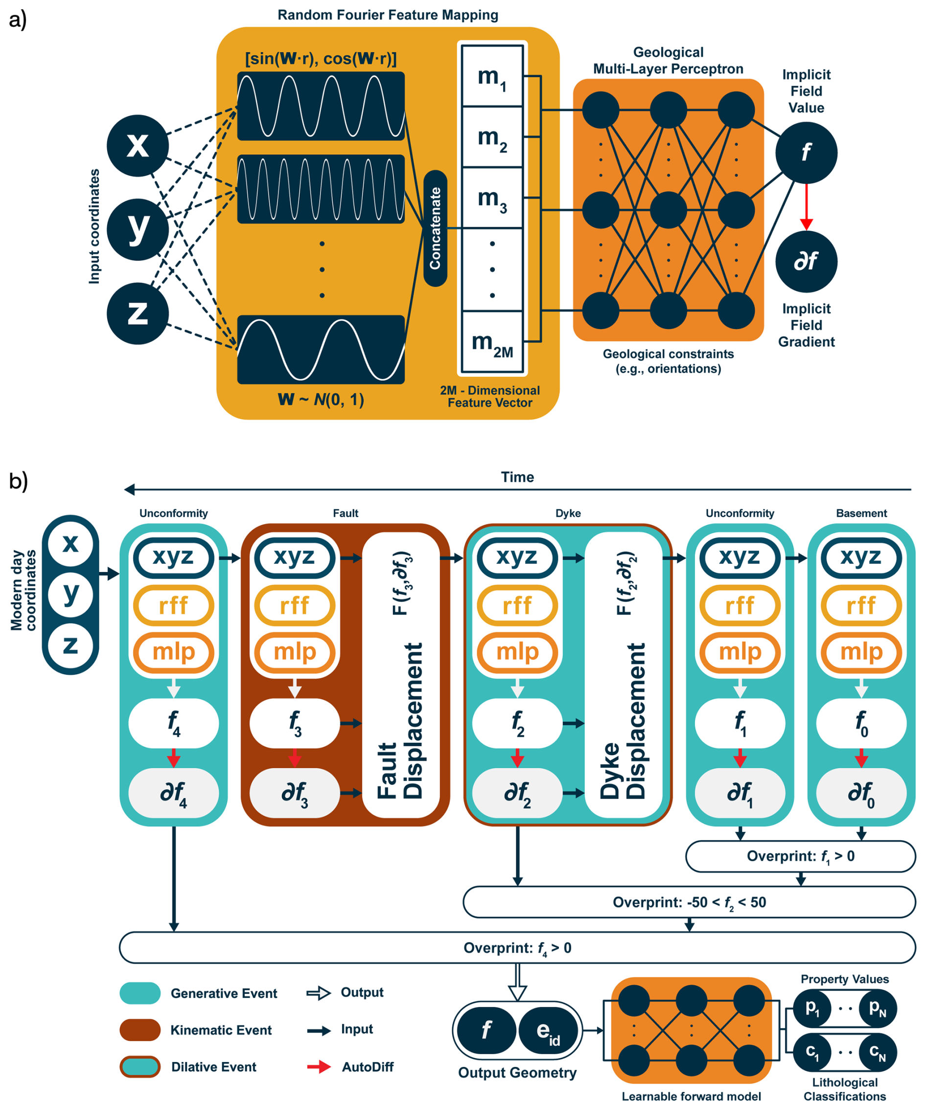
Figure 1 Overview of the curlew geological modeling approach, which combines (a) Random Fourier Feature (RFF) mappings, which transform input (spatial) coordinates into higher-dimensional Fourier features, with neural fields (multi-layer perceptrons) to predict implicit field values and gradients, guided by geological constraints. Different geological structures are each parameterised with their own neural field, such that a model is constructed from a temporally sequential combination of events (e.g., unconformities, faults, and dykes). Generative (stratigraphic deposition), kinematic (fault displacement), and dilative (dyke intrusion) events are chained through differentiable relationships, allowing integrated modeling and semi-supervised updates via a learnable forward model informed by quantitative property data and lithological classifications.

This RFF approach enhances the model's ability to learn high-frequency geological features. Furthermore, the encoding introduces inherent stochasticity into the interpolation process. Models trained with different seeds will learn different representations of the subsurface geometry for the same constraints, due to the random nature of the projection directions. Therefore, we can generate model ensembles by changing the seed of the random number generator to get different projections for each model. This becomes useful for stochastic uncertainty estimation, as multiple outputs can be generated without perturbing the input data (as is typical in established approaches; e.g., Wellmann and Regenauer-Lieb, 2012). In specific cases, it theoretically also allows known information on e.g., fold wavelength to be indirectly integrated as a model parameter by seeding the Fourier frequencies (and potentially directions) according to measured fold geometry.

The RFF encoding is followed by a standard multi-layer perceptron (MLP). The MLP block applies non-linear activation functions to all hidden layers. Because our framework computes derivatives via automatic differentiation (AD), the chosen activations must be C² differentiable (as the network requires a second backward pass for the optimisation). Functions lacking this property, such as ReLU, produce abrupt edges in the resulting interpolation. Even among C² differentiable options, performances may vary. For instance, the hyperbolic tangent (TanH) is stable, but its second-order derivatives are small and prone to saturation, which can impede convergence. Empirical testing showed that Swish (SiLU, Ramachandran et al., 2017) and Mish (Misra, 2019) provided the best overall results. We have also experimented with options in which the Fourier features are directly connected to the predicted scalar field with a single layer of neurons (i.e. with no hidden layers and no activation functions). Early tests suggest that this minimalist neural field performs well in many situations, so we suggest that this architecture is used as a starting point (and extra complexity is added only if needed).

3.2 Loss functions

A neural field stores the implicit field within the weights and biases of the MLP block. These weights and biases are trained using a combination of local and global losses (the RFF projection remains fixed after initialisation). Local losses are accumulated at specific coordinates for which there is information on the implicit field value, its gradient, or its relation to other points in the model (see Sect. 2.2). Global losses are accumulated either over a grid of points that covers (or extends slightly beyond) the model domain, or (typically) on points that are randomly sampled from a grid during each training epoch. We have implemented loss functions in curlew such that each of these aspects can be introduced via corresponding hyperparameters. However, we recommend that any specific neural field should only use two to four of these loss functions (usually a local/relational loss coupled with a global loss), with the remaining terms disabled by setting their corresponding hyperparameter to zero. Every additional loss term adds an extra objective for the optimiser to minimise, quickly turning the interpolation into a complicated multi-objective optimisation problem (see Sect. 5.3).

3.2.1 Local losses – geological data

Each local constraint is defined by a coordinate and a value, represented in curlew as pairs of arrays to allow vectorised pytorch (Paszke et al., 2019) operations. The input coordinates can be presented in any Euclidean coordinate system (e.g., UTM) as the feature mapping has a normalisation effect. The values can represent known stratigraphic position (value constraints), younging direction (gradient constraints) or strike and dip (tangent constraints). Therefore, the local loss ℒ_l is

$$\begin{array}{}\text{(2)}& {\mathcal{L}}_{\mathrm{l}}=\stackrel{\text{Value Loss}}{\overbrace{\mathit{\alpha }\Vert f_{{\mathrm{p}}_{\mathrm{1}}}-f_{{\mathrm{c}}_{\mathrm{1}}}{\Vert }_{\mathrm{2}}}}+\stackrel{\text{Gradient Loss}}{\overbrace{\mathit{\beta }\Vert {\widehat{\mathit{g}}}_{{\mathrm{p}}_{\mathrm{2}}}-{\widehat{\mathit{g}}}_{{\mathrm{c}}_{\mathrm{2}}}{\Vert }_{\mathrm{2}}}}+\stackrel{\text{Tangent Loss}}{\overbrace{\mathit{\gamma }\left(\mathrm{1}-\left|{\widehat{\mathit{g}}}_{{\mathrm{p}}_{\mathrm{3}}}\cdot {\widehat{\mathit{g}}}_{{\mathrm{c}}_{\mathrm{3}}}\right|\right)}}\end{array}$$

where f refers to the implicit field value and $\widehat{\mathit{g}}$ refers to the normalised implicit field gradient. The subscripts p and c refer to the predicted and constraint (measured) terms, $\Vert \cdot {\Vert }_{\mathrm{2}}$ is the L2 norm, and α, β, and γ are the corresponding hyperparameters. As with any multi-objective optimisation problem, careful selection of these hyperparameters can be crucial for achieving good results. Also note that where the absolute direction of the gradient is unknown, the tangent loss accumulates errors proportional to the angular distance between the predicted and measured orientation axes by maximising cosine similarity.

Relational constraints (inequalities and equalities) are implemented using a computationally efficient approach that randomly samples P pairs of points from the left- and right-hand sides of each (in)equality. This avoids needing to construct a large pairwise difference matrix, which would be prohibitively expensive for large datasets, and is analogous to widely used mini-batch approaches used when training deep learning models. Thus, if we construct a difference term $\mathrm{\Delta }=f_{\mathrm{p}\in \text{LHS}}-f_{\mathrm{p}\in \text{RHS}}$, the relational loss term ℒ_r can thus be expressed as:

$$\begin{array}{}\text{(3)}& \begin{array}{rl}{\displaystyle }& {\displaystyle }{\mathcal{L}}_{\mathrm{r}}=\\ {\displaystyle }& {\displaystyle }\left\{\begin{array}{ll}\mathit{\lambda }\Vert \mathrm{\Delta }{\Vert }_{\mathrm{2}}& \forall \text{LHS}=\text{RHS},\text{Contact equality}\\ \mathit{\lambda }min(\mathrm{\Delta },\mathrm{0})& \forall \text{LHS}>\text{RHS},\text{Above contact inequality}\\ \mathit{\lambda }max(\mathrm{\Delta },\mathrm{0})& \forall \text{LHS}<\text{RHS},\text{Below contact inequality}\end{array}\right.\end{array}\end{array}$$

where LHS and RHS refer to the set of points sampled above and below a specific geological interface (inequalities), or along a single interface (equalities), and λ is the corresponding hyperparameter. The first case in Eq. (3) corresponds to the equality constraints, where N points are drawn randomly from the LHS and RHS sets each (i.e. N pairs), and the absolute difference between the predicted implicit field values at these points is minimized. The remaining cases correspond to the inequality constraints, where the clamp function is used to ignore differences above or below 0, as per the direction of the inequality.

3.2.2 Global losses – geological rules

Global losses control more general properties of the interpolated implicit field. This can be used to e.g., encourage constant gradient (resulting in geological units that minimize changes in thickness) or discourage geologically implausible closed isosurfaces (bubbles). Unlike local losses, they are not related to any specific data, and are evaluated on either a grid of points covering the model domain, or at a set of N points chosen randomly across the model domain during each epoch. We have currently implemented three global losses (ℒ_g) in curlew: flatness loss, thickness loss and monotonicity loss. These can be written as:

$$\begin{array}{}\text{(4)}& \begin{array}{rl}{\displaystyle }{\mathcal{L}}_{\mathrm{g}}& {\displaystyle }=\stackrel{\text{Flatness Loss}}{\overbrace{\mathit{\eta }\Vert {\widehat{\mathit{g}}}_{\mathrm{p}\in G}-{\widehat{\mathit{g}}}_{\text{trend}}{\Vert }_{\mathrm{2}}}}+\stackrel{\text{Thickness Loss}}{\overbrace{\mathit{ϵ}\left({\displaystyle \frac{\text{Var}\left(\Vert {\mathit{g}}_{\mathrm{p}\in G}{\Vert }_{\mathrm{2}}\right)}{\mathbb{E}[\Vert {\mathit{g}}_{\mathrm{p}\in G}{\Vert }_{\mathrm{2}}{]}^{\mathrm{2}}}}\right)}}\\ {\displaystyle }& {\displaystyle }+\stackrel{\text{Monotonicity Loss}}{\overbrace{\mathit{\kappa }\left|\mathrm{\nabla }\cdot \left({\widehat{\mathit{g}}}_{\mathrm{p}\in G}\right)\right|}}\end{array}\end{array}$$

where G is the set of grid points sampled in each epoch, ${\widehat{\mathit{g}}}_{\text{trend}}$ is the user-defined global gradient trend, ∇(⋅) is the divergence operator, and η, ϵ, and κ are the corresponding hyperparameters. Flatness loss acts as a (weak) gradient constraint on each grid point to encourage unconstrained parts of the implicit field to have a specific orientation. The thickness loss penalises the relative deviation of gradient magnitudes from their mean, encouraging a uniform and non-zero gradient magnitude (i.e. constant thickness). It is equivalent to minimising the squared coefficient of variation (CV²) of the gradient norm – that is, the variance normalised by the squared mean – making the penalty scale-invariant.

Finally, we have implemented a loss that discourages local maxima and minima (bubbles) in the interpolated implicit field. This ‘monotonicity' loss is defined as the divergence of the normalised (unit length) gradient vector field. Rather than directly penalizing the Laplacian (which would aim for an ideal harmonic implicit field), we adopt a curvature-based divergence regulariser, by using normalized gradients. This approach is analogous to total variation regularisation (Rudin et al., 1992) and mean curvature flow formulations (Osher and Sethian, 1988), and in this context helps to preserve geological interfaces and prevents the formation of spurious internal extrema, as recently demonstrated for neural field applications (Gropp et al., 2020; Sitzmann et al., 2020). To save memory, the second derivative (hessian) matrices used to compute the monotonicity loss are estimated numerically. This numerical estimation also allows us to have an external control on the scale of curvatures we want to minimise, by controlling the size of the grid-step used to numerically compute the hessian.

3.3 Generative and kinematic events – a framework for combining neural fields

The aforementioned sections explain the constraints and controls over the interpolation of a single, smooth, and continuous implicit field. However, most SGMs contain multiple geological events, separated by unconformable, intrusive or faulted contacts. Each of these events typically need to be represented using their own interpolated implicit field, before temporally guided intersections are used to derive a combined model (Grose et al., 2021a; Wellmann and Caumon, 2018).

In curlew, this is achieved using overprint and/or offset relations (Fig. 1b). Therefore, most neural fields in a model built using curlew represent a geological event (Table 1) that (1) creates new units (generative events, such as e.g., depositions or intrusions) or (2) displaces older units (kinematic events, such as faults). Sheet intrusions (e.g., dykes) are an example of events that do both – generate a new unit (the dyke fill) while displacing the older units (due to opening along the dyke).

Table 1 Overview of structural fields available in curlew, highlighting generative and kinematic components. Domain boundaries partition the model into separate domains, each governed by distinct implicit fields or chains of implicit fields (L, G).

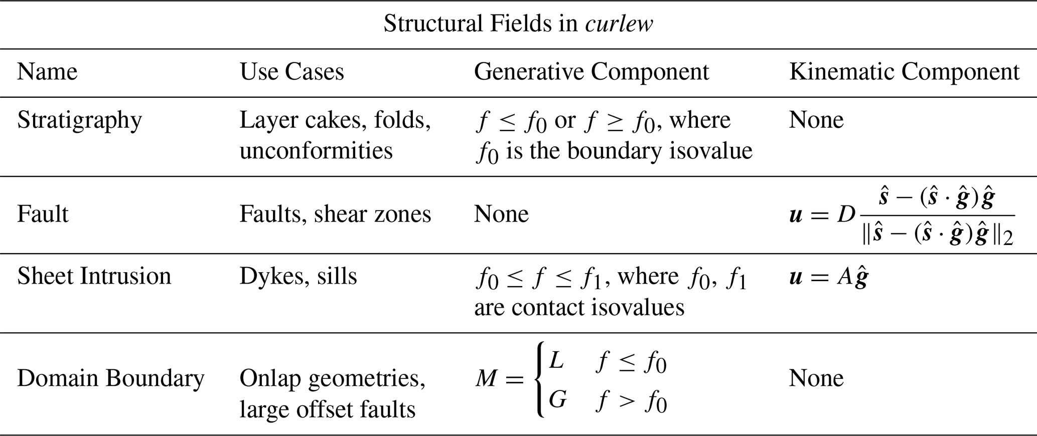
f: Implicit field value; $\widehat{\mathit{g}}$: Implicit field gradient direction; $\widehat{\mathit{s}}$: Shortening direction; D: Fault offset; A: Sheet aperture; u: Displacement.

Generative events in curlew are combined with older ones using an inequality: implicit field values representing deposition above an unconformity “overprint” older values where they exceed a threshold value, and values defining a dyke overprint older values within a specified range (proportional to the dyke aperture). Conversely, kinematic events define vector displacements (based on the gradient-direction and/or tangent plane of the interpolated implicit field) that retro-deform the input coordinates used to constrain (or evaluate) older fields. Importantly these vector displacements are differentiable, allowing the combined training of multiple neural fields to learn additional unknown parameters (e.g., fault slip magnitude).

Overprint relations are implemented using a differentiable sigmoid function, such that values from a younger implicit field replace those of older ones based on an inequality. For unconformities, this inequality specifies a basement value below which the interpolated values are ignored (to retain predictions of basement lithology from older neural fields). An Event ID (e_id, see Fig. 1b) is assigned to each overprinted location to keep track of the neural field that generated each implicit field value (and distinguish regions representing e.g., the interior of a dyke from those representing the surrounding stratigraphy). The geological operators outlining the implementation of kinematic events in curlew are outlined in the following sections, though terminology for these operations varies across the literature (Grose et al., 2021a, b; Calcagno et al., 2008; Hillier et al., 2023)

3.3.1 Faults

Faults are implemented in curlew using displacement fields. These fields modify existing geological structures by offsetting them along geologically plausible slip directions. The displacement direction is determined based on the interaction between the regional stress field and the local geometry of the fault surface.

Specifically, the slip direction vector $\widehat{\mathit{u}}$ is computed by projecting a vector representing the maximum shortening direction $\widehat{\mathit{s}}$ onto the plane perpendicular to the normalised gradient $\widehat{\mathit{g}}$ of the implicit field defining the fault surface:

$$\begin{array}{}\text{(5)}& \widehat{\mathit{u}}={\displaystyle \frac{\widehat{\mathit{s}}-(\widehat{\mathit{s}}\cdot \widehat{\mathit{g}})\widehat{\mathit{g}}}{\Vert \widehat{\mathit{s}}-(\widehat{\mathit{s}}\cdot \widehat{\mathit{g}})\widehat{\mathit{g}}{\Vert }_{\mathrm{2}}}}.\end{array}$$

Here, the term $(\widehat{\mathit{s}}\cdot \widehat{\mathit{g}})\widehat{\mathit{g}}$ gives the component of the shortening vector normal to the fault plane. Subtracting this from $\widehat{\mathit{s}}$ yields the component tangential to the fault, ensuring that the resulting slip direction is (locally) fault-parallel and consistent with mechanical considerations (Fig. 2a). The resulting vector is then normalised to give a unit slip direction vector $\widehat{\mathit{u}}$ that can be scaled by the desired displacement magnitude (D) to produce the final displacement vector u.

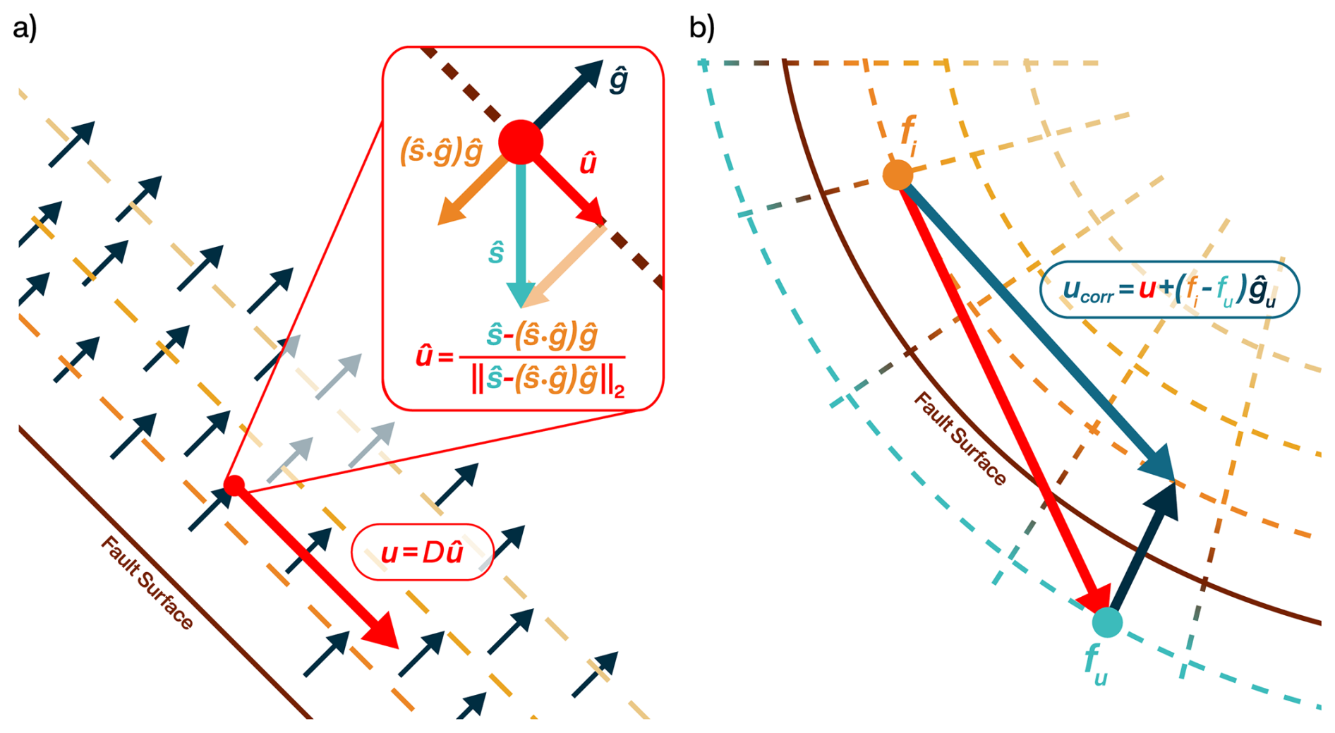
Figure 2 Fault displacement in curlew. The displacement direction at every point is calculated by projecting the (pre-defined) shortening direction $\left(\widehat{\mathit{s}}\right)$ onto the tangent plane of the implicit field that defines the fault geometry (a). The resulting displacement direction vector $\left(\widehat{\mathit{u}}\right)$ is then scaled by the (optionally learnable) offset magnitude (D) to derive a displacement vector (u). For curved fault systems (i.e., where the curvature of the fault plane is relevant with respect to the fault offset), curlew offers an optional correction (b), which uses the difference between the implicit field values at the displaced and initial locations, to project the point back onto the initial isosurface. This approximation results in some change in the displacement magnitude, but for most realistic fault geometries this error is negligible.

For infinite faults, the magnitude is defined by a single scalar value (optionally learnable). For finite faults, the magnitude would need to vary as a function of distance from the fault center – following empirical displacement profiles (Grose et al., 2021b, a). Once the displacement vector is determined, its direction (sign) is assigned by applying two sigmoid functions that impose opposite slip directions on either side (hangingwall and footwall) of the fault. The sharpness of the sigmoid can be tuned to simulate either brittle fault behavior (sharp transition) or ductile shear zones (smooth transition), enabling the generation of simple drag folds adjacent to brittle faults.

For highly curved (with respect to displacement magnitude) faults, curlew applies an optional gradient correction to correct for curvature in the displacement vector between the initial and displaced positions (Fig. 2b). This correction ensures that displaced points remain (approximately) on the same isosurface of the fault implicit field, and is given by:

$$\begin{array}{}\text{(6)}& {\mathit{u}}_{\text{corr}}=\mathit{u}+(f_i-f_u){\widehat{\mathit{g}}}_{\mathrm{u}}\end{array}$$

where ${\widehat{\mathit{g}}}_{\mathrm{u}}$ is the gradient unit vector at the displaced location, f_i and f_u are the implicit field values at the original and displaced positions, respectively. The term $(f_i-f_u){\widehat{\mathit{g}}}_{\mathrm{u}}$ projects the scalar mismatch back along the gradient, correcting for small misalignments introduced by displacement in regions of high curvature or gradient variation.

3.3.2 Sheet intrusions

Sheet intrusions, such as dykes and sills, are implemented using the logic of both generative and kinematic implicit fields. These fields create the new geological units (solidified magma), and displace older ones to account for dilation during intrusion.

The generative component uses an overprinting relationship defined between an upper and lower scalar bound, assigning new implicit field values (and event IDs) between two isosurfaces that represent the intrusion contacts. An offset function is also defined to move pre-existing structures outward, in the direction of the gradient of the intrusion's implicit field. The gradient is flipped – based on the sign of the implicit field – so that vectors consistently point away from the intrusion's centerplane, which is represented by the zero isosurface. An aperture term scales the gradient's magnitude to reflect the intrusion's thickness.

3.4 Domain boundaries – multi-domain structural models in curlew

The final structural element implemented in curlew is the domain boundary, which enables the segmentation of geological models into distinct sub-domains, each governed by its own sequence of (older) geological events. Domain boundaries thus partition the model into separate neural field chains, based on inequalities defined on the domain boundary implicit field, and can be combined to construct complex geological structures and relations.

A typical use case arises when sedimentary units are deposited above an unconformity but pinch-out laterally (onlap geometries). Because such deposits do not follow the generative logic of a conformal event (i.e., they are not stratigraphically contiguous with the unconformity), they cannot be represented within a single event chain. Instead, the unconformity is defined as a domain boundary, which splits the model into two stratigraphically and structurally independent domains: one below the unconformity and one above it.

Another key application of domain boundaries is in the modelling of major fault zones. When a fault induces large displacement, or juxtaposes basement rock against cover sequences, the stratigraphic relationship between the foot- and hanging-wall often becomes unresolvable. For such structurally complex settings, the fault is most simply defined as a domain boundary separating sub-models with different geological histories.

This formalism allows curlew to integrate geologically inconsistent or discontinuous regions within a unified framework. It removes the need for users to manually partition their models or construct separate simulations for each geological block, and facilitates instances where domain boundaries are affected by younger deformations (e.g. faults).

4 Results

We have applied curlew to a set of synthetic examples that explore the various capabilities of our neural field based interpolation approach, and illustrate different aspects of the underlying loss function. These are presented in the following sections, followed by an application to a real example constrained by data extracted from a digital outcrop model from Newcastle, Australia.

To help document and introduce potential users to specifics of the curlew modelling approach, each of these examples is provided as a jupyter notebook (see Code and Data availability section).

4.1 Folded stratigraphy

To illustrate the various loss terms described above, and to showcase the importance of the length scale parameter used during the Fourier feature projection, we have generated a simple test model containing a folded stratigraphic sequence (Fig. 3). This model involves two generations of folding events, a small wavelength small amplitude folding overprinted on large wavelength large amplitude folds. A Fourier series was used to generate similar folds with relatively sharp noses (Fig. 3a). This sequence was then sampled along hypothetical boreholes (Fig. 3b) to simulate gradient, value and tangent constraints. Note that while this synthetic example is 2D for ease of visualisation, all of the aforementioned methods (and the successive results) could be applied in 3D too.

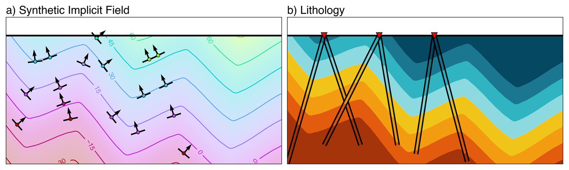
Figure 3 Synthetic (analytical) geological model simulating a folded stratigraphy. The implicit field (a) was sampled to derive gradient orientations (arrows) and implicit field values (circles) as constraints for a subsequent interpolation. Isosurfaces extracted from the implicit field at predefined seed positions also give a stratigraphic classification (b), which were used to define relational constraints. The red triangles represent the locations of the boreholes along which the constraints were sampled.

4.1.1 Local, relational and global losses

We used different combinations of constraints and losses to show the effect of each part of our loss function (Eqs. 2–4) on the interpolated result (Fig. 4). To start, we fit a neural field model using each constraint type in isolation (Fig. 4a–d), without any additional global losses. The results show that tangent constraints (Fig. 4a) on their own are (unsurprisingly) extremely weak, since they only encode the axis of the gradient. This results in closed isosurfaces (i.e. “bubbles”), where the implicit field curls back on itself due to the undefined direction of the gradient.

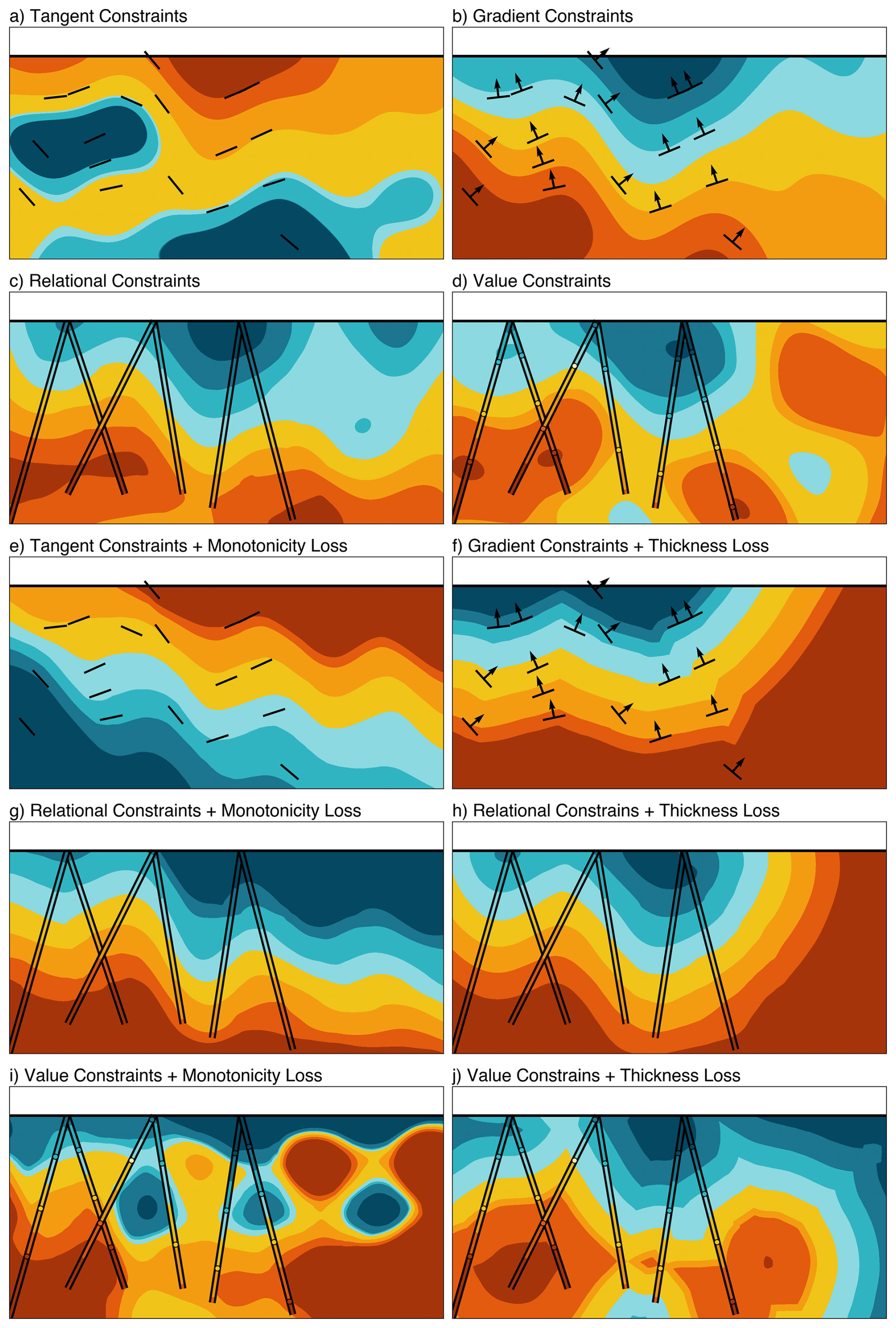
Figure 4 Interpolated stratigraphy for different combinations of constraints and losses, using the same network architecture (1 layer, 512 neurons), 2000 training epochs, and two (150, 1000) length scales. An early stopping criterion was applied to stop training after 100 epochs with less than 10⁻⁴ improvement in the loss. The individual models show results using tangent constraints (a), gradient constraints (b), relational constraints (c), and value constraints (d) in isolation. The addition of monotonicity loss to tangent constraints (e) and the thickness loss to the gradient constraints (f) improves the resulting interpolation. The flexibility afforded by relational (g, h) rather than value (i, j) constraints also seems to help the model converge to a more geologically realistic solution.

This is partially resolved when gradient constraints are used (Fig. 4b). The isosurfaces are now close to monotonic, as the directionality encoded in the gradient constraints forces the implicit field to “flow” from the bottom to the top of the model. However, away from the data, the interpolated field behaves randomly, and includes geologically unlikely variations in gradient magnitude (changes in thickness).

The use of equality and inequality (relational) constraints (Fig. 4c) results in a smoothly undulating model that correctly matches all of the contacts sampled by the boreholes, as well as maintaining correct stratigraphic relationships across the domain. Interestingly, however, the use of value constraints results in a very different interpolation (Fig. 4d) in which the neural field accurately reproduced the values at constraint locations but created artefacts (such as bubbles) elsewhere.

Introducing the monotonicity loss removes the bubble artefacts from results obtained with the aforementioned constraint types (Fig. 4e and g), but produces an interpolation with potentially unrealistic variations in unit thickness. The monotonicity loss seems to require further fine tuning in combination with value constraints (Fig. 4i).

Use of the thickness loss term resulted in an interpolation that honours unit thickness (class 1B parallel folds), giving geologically plausible models in combination with gradient and relational constraints. In combination with value constraints, however, the neural field found a solution dominated by angular bubbles that we consider to be unreasonable.

These additional global losses thus prove to be extremely useful in constraining the model in areas lacking local constraints, and can be adapted to enforce various geological rules. Interestingly, the global losses also appear to work best with relational constraints (inequalities), rather than value constraints.

4.1.2 Length scales

The synthetic folds model also allows us to explore one of the most important parameters for our implementation of a neural field interpolator: the length scale used during the Fourier feature encoding (cf. Sect. 3.1). To show the impact of different length scales, we used relational and gradient constraints in combination with a global monotonicity loss while varying only the length scales used by the neural field (Fig. 5).

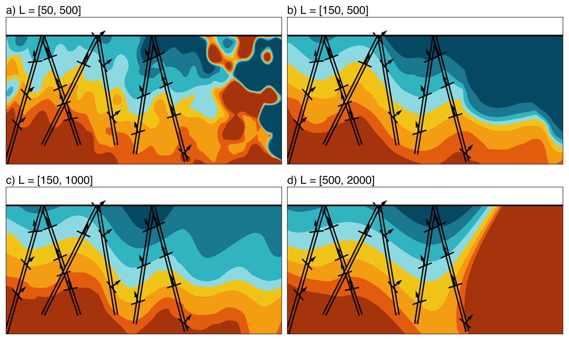
Figure 5 Interpolated stratigraphy for different pairs of length scales (but retaining the same settings as Fig. 4). Small length scales (a) result in over-fitting and random artefacts away from the data, whereas large length scales (d) result in under-fitting. Note also that the model is most influenced by the smaller length scale (as seen in b and c), whereas the larger length scale likely has more influence on large scale trends.

The resulting models highlight the importance of choosing appropriate length scales. Scales that are too small (Fig. 5a) result in severe over-fitting and largely meaningless predictions away from the data. Conversely, when the length scale is too large (Fig. 5d), the neural field under-fits and cannot make accurate predictions at the constraint locations, due to its limited capability to learn higher frequency variations.

For this example, the length scales of (150, 500) seems to be a good trade-off between fitting the data and avoiding random overfitting artefacts (Fig. 5b). A comparison of Fig. 5b and c suggest that the results are most heavily influenced by the smaller length scale (while the large length scale serves to reproduce the overall trend and so is less sensitive, albeit still important). As a rule of thumb, the longest length scale should be 4 times the longest model dimension, while the shortest should be determined by the data spacing.

4.2 Combining multiple neural fields

Only the simplest geological models can be represented by a single implicit field. Hence, we develop a second synthetic model that highlights curlew's approach to fault displacement, dyke injection and the use of domain boundaries to model intrusive and onlap relations (Fig. 6a). The implicit fields associated with the depositional and kinematic events of the model are generated using predefined analytic equations, allowing us to construct a completely synthetic model for testing. Seed locations within these implicit fields were used to define isosurfaces that mimic stratigraphic contacts (Fig. 6b). Value and gradient constraints were sampled from each implicit field along vertical drill holes, to be used as synthetic data (Fig. 6d–j) when fitting (training) an interpolated neural field based model. Every individual field in the model influences every field that came before it with displacements, overprinting, or a combination of both actions (Fig. 7c).

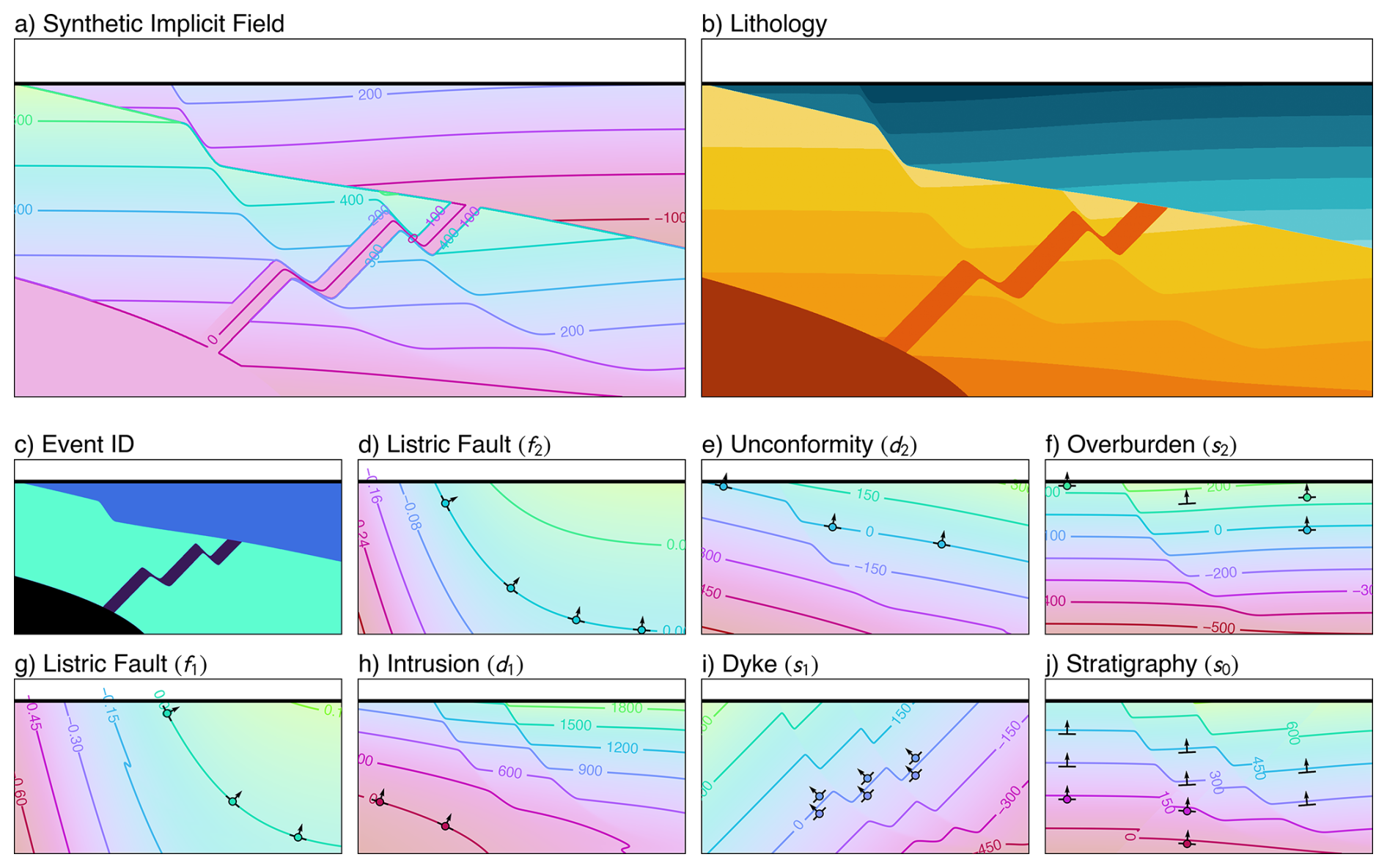
Figure 6 A structurally complex analytical synthetic model built in curlew. The resulting implicit field (a), corresponding lithology (b), and event ID (c) are also shown. This model represents a sequence of seven geological events, starting with a “layer cake” stratigraphy (j). Subsequently, this stratigraphy is intersected by a dyke (i), and intruded by a stock in the lower left corner of the model domain, represented through a domain boundary (h). The intrusion is assigned an arbitrary implicit field value (in this case −2) as its boundary is the only relevant entity. A listric fault then cuts through the units (g) followed by an unconformity that erodes through the deposited sequence, which is overlaid by a secondary deposition (f). As the deposited unit is not conformable to the unconformity surface (i.e., onlap), the unconformity is also modelled as a domain boundary (e). Finally, a second listric fault (d) cuts through the entire sequence.

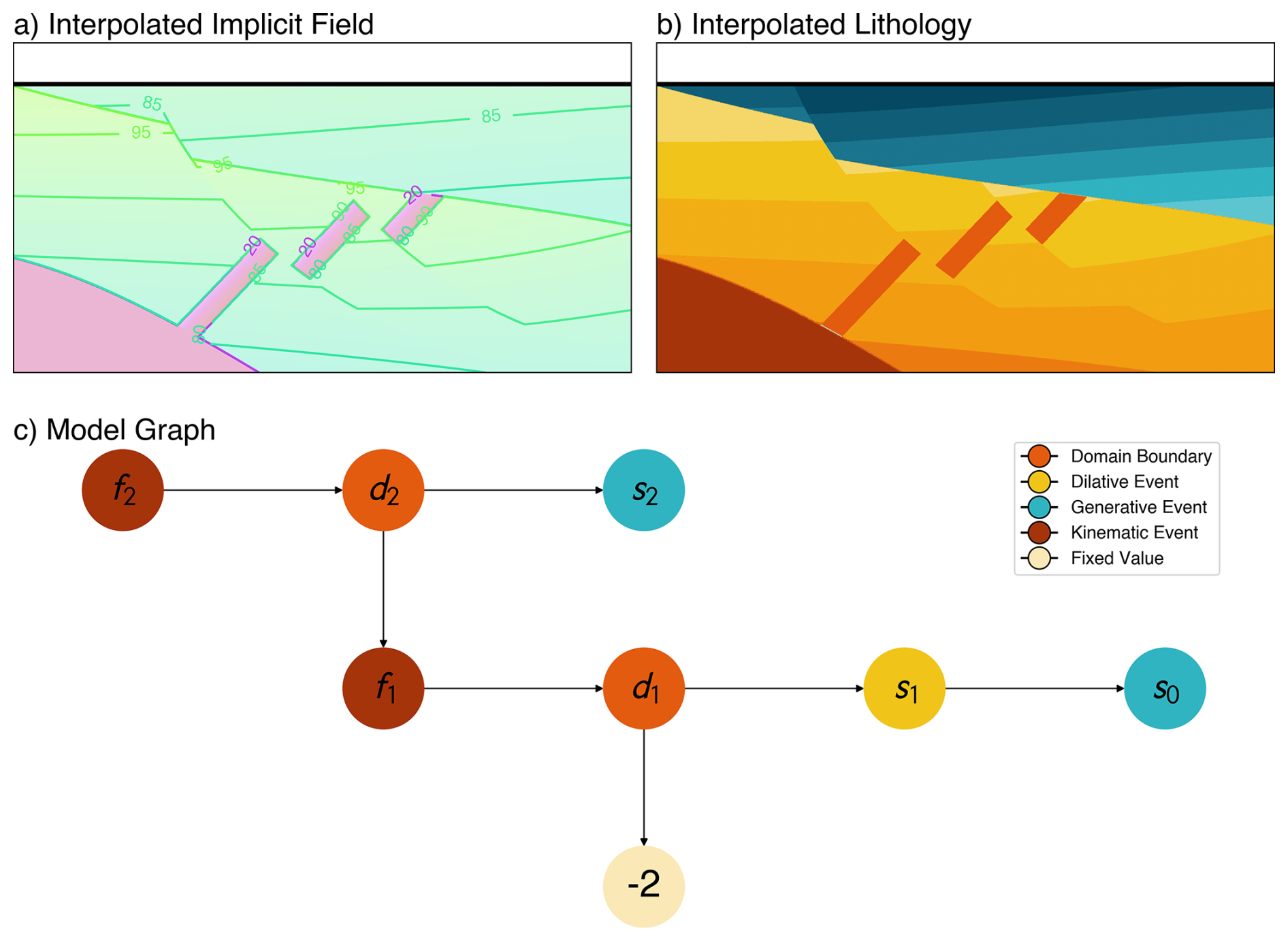
Figure 7 Interpolation results (a) and corresponding lithology classification (b) derived by fitting a network of neural fields (c) to the sparse constraints shown in Fig. 6. As mentioned earlier, the intrusive body is represented by a constant scalar field value (−2 in this case) as only the boundary of the intrusion (defined by the domain boundary field) is of interest.

A neural field was parameterised (with different hyperparameters for various losses) for each set of constraints. The gradient loss term for all the implicit fields was given a higher weight, to give more importance to the shape of the reconstructed model. For the depositional events (s₀ and s₂), the value loss was given a very low weight (as the values are arbitrarily defined and may impede convergence), and the monotonicity loss enabled used to encourage a bubble-free geometry. For the dyke, as the values determine the aperture of the dyke, the value loss was enabled, along with the thickness loss, to ensure it retains a constant thickness in interpolated regions. Finally, the domain boundaries and faults were fit by prioritising value-loss in combination with a thickness loss that acts to keep a constant implicit field gradient. For this example fault-displacement was assumed to be known, so the principal shortening direction ($\widehat{\mathit{s}}$) and slip magnitude were defined a-priori (though the slip magnitude can also be treated as a learnable parameter, as shown in the following section).

After 1000 epochs of training, the interpolated curlew model closely matches the original synthetic one, with a few visible differences (Fig. 7). The implicit values for the two models are very different (0–600 vs. 80–100 for s₀), but this is coherent with the disabled value loss function for these two fields and does not necessarily influence the isosurface geometry (given we extract the isosurfaces for the lithologies based on seed positions).

4.3 Digital outcrop reconstruction

Finally, to demonstrate that curlew can be applied to real (3D) data, we present a model generated from a digital outcrop in Australia. The digital outcrop consists of a faulted stratigraphic sequence intruded by a dyke. The Compass plugin for CloudCompare (Thiele et al., 2017) was used to extract (1) traces along the contacts between the stratigraphic units, dyke margin and fault surface, and (2) orientation measurements (strike and dip) of each of these geological structures.

Since these traces included a large number of points (due to the high resolution of the point cloud), they were subsampled to acquire evenly-spaced points along the stratigraphic contacts, the fault surface, and the dyke (Fig. 8a). While these traces could be directly used as relational constraints, we used the subsampled points as value constraints, with the values being the approximate height of the layer from the base of the digital outcrop. These constraints were then used to constrain three consecutive neural fields: (1) a stratigraphic field, (2) a fault field, and (3) dyke field.

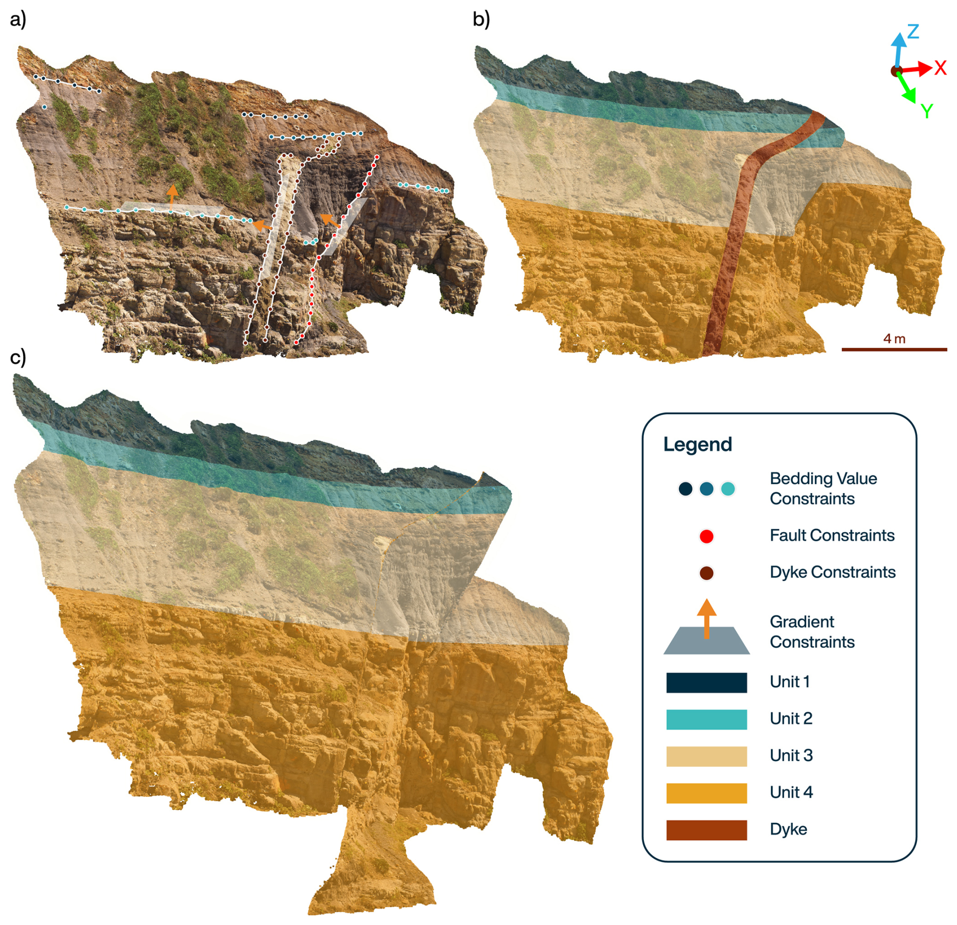
Figure 8 Interface and gradient constraints extracted from a digital outcrop model (a) from Newcastle, Australia. These were used to construct a 3D curlew model describing the main geological structures and stratigraphic units and derive a lithological classification (b), plotted here as an overlay on the original RGB colours for clarity. The fitted displacement fields from the curlew model were also used to offset these points and remove displacement from the dyke and fault, resulting in an undeformed point cloud closer to the original depositional geometry (c).

After fitting each neural field separately to generate an initial geometry, we froze the geometries of the fault and dyke fields by fixing the weights of their corresponding neural fields. The fault slip and stratigraphic interpolation were then fit simultaneously, to find an optimal displacement for the fault (i.e. by finding the fault offset that results, after reconstruction, in the smoothest interpolation of the older stratigraphy field).

The resulting model (Fig. 8b) and solutions to the displacement fields induced by the fault and the dyke were then used to “undeform” the outcrop and retrieve pre-deformation locations for all of the points in the digital outcrop model (Fig. 8c). Note that while the dyke in the original outcrop is finite, the modelled dyke is infinite. Finite dykes (and faults) are planned to be implemented in future versions of curlew.

5 Discussion

We have presented an open-source python package, curlew, which leverages neural fields to generate implicit geological representations of structural geological models. The neural field approach employed by curlew is highly versatile and adaptable, capable of handling a wide range of constraint types, data modalities, and loss functions. Its representation of structural geological models in a fully differentiable architecture, and the ability of the underlying neural fields to arbitrarily adapt the geometry they represent, opens the door to a variety of new approaches to common earth modelling, property field interpolation and geophysical inversion.

Similarly to radial basis functions (RBF) or co-kriging approaches, models built with curlew are entirely meshless. Once trained, they can be evaluated at arbitrary locations, facilitating advanced methods for contour extraction or adaptive gridding strategies. Furthermore, given its pytorch core, training and inference operations are GPU-parallelised and scalable on large computing infrastructure. This contrasts against established methods such as co-kriging and RBF, which scale poorly with increasing data volume. Specifically, the requirement to invert a dense N×N covariance or interpolation matrix incurs a cubic computational cost (𝒪(N³)), making these methods inefficient without numerical simplifications like compactly supported kernels, fast multipole methods, or domain decomposition (Rasmussen and Williams, 2005; Cavoretto et al., 2016; Beatson et al., 2001; Wendland, 1995).

The differentiable nature of the generated models also means model outputs can include the gradient of the underlying implicit fields (i.e. structural orientation measurements), and if necessary, higher order derivatives (e.g., curvature) through automatic differentiation (although the second order derivatives are computed numerically in curlew for computational scalability). As shown in Sect. 3.2.2, this has been leveraged to suppress (albeit not eliminate) common interpolation artefacts such as “bubbles”, and further applications are envisaged when interpolating property fields (e.g., permeability, ore grade) given a structural geological model.

Curiously, our experiments also suggest that, in the context of geological modelling with neural fields, the inclusion of value constraints (instead of somewhat equivalent inequality constraints) can make it difficult for neural fields to converge to a geologically realistic geometry. This behaviour might be explained by the under-determined nature of gradient-only constraints – the network's loss is invariant to adding a constant offset to the field. Thus, the optimisation has a flat direction, yielding a continuum (valley) of equally valid solutions rather than a single narrow optimum. By contrast, specifying exact field values removes this degeneracy, collapsing the solution space to isolated optima that are much harder to find. Prior work in neural network training has noted that having such flat minima or degenerate solution manifolds can make optimisation easier and models generalise better (Li et al., 2017). Through their work on Sobolev Training, Czarnecki et al. (2017), further demonstrate that leveraging derivative information (gradients) in training leads to improved learning efficiency, implying that matching the shape of the target function is often more tractable than matching exact values.

5.1 Random Fourier Features

The inclusion of Random Fourier Feature (RFF) mapping allows curlew to train neural fields without using the pre-training protocol outlined by Hillier et al. (2023) for network weight initialisation. Although there are several alternative approaches that could behave similarly (e.g., SiREN; Sitzmann et al., 2020), the RFF mapping has the advantage that length-scales used by the interpolator can be carefully controlled, and potentially seeded for specific geological settings (e.g., in folded rocks with known amplitude and axial plane). However, this sensitivity can also be a disadvantage, as the manual selection of appropriate length scales can be quite challenging.

Interestingly, the randomness inherent to RFF mapping means multiple model realisations can be obtained by training models on the same data but with different RFF seeds (Fig. 9). While model ensembles can also be derived from conventional neural fields, we suspect that the significant differences in (learned) geometric representation that result when randomly sampling different RFFs enable greater exploration of the potential solution space. The precise meaning of these variations remains a topic of future research, but it could facilitate methods for quantifying the epistemic uncertainty of the interpolated result.

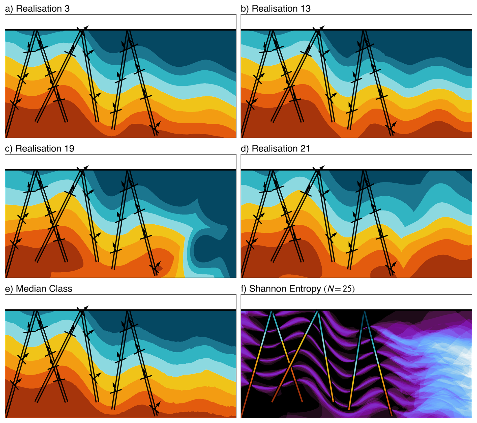
Figure 9 Selected realisations (a–d) from an ensemble of 25 curlew models derived using different random seeds for the RFF encoding. The median predicted class (e) highlights the predominance of geologically plausible solutions. The Shannon information entropy of the predicted classes (f) shows high uncertainty (brighter colour) at the fold hinges and away from the drill hole data, suggesting this approach might be used to meaningfully quantify model uncertainty.

For example, we have generated 25 random realisations of the folded stratigraphy model (see Sect. 4.1) and computed the information entropy (Shannon, 1948) of the resulting lithology predictions (Fig. 9f). This clearly highlights increased uncertainty near fold hinges and away from the constraints, aiding interpretation and potentially facilitating targeted data collection (Tacher et al., 2006; Wellmann et al., 2010, 2014; Wellmann and Caumon, 2018).

A full-variational Bayesian Neural Network (BNN; Goan and Fookes, 2020) provides a first order uncertainty quantification, as the weights and biases of the neural network are not fixed values and can be approximated as probability distributions. Thus, this more comprehensive representation of variability may help to capture epistemic uncertainty arising from the data. However, BNNs are computationally expensive, even more than the ensembles for highly optimised networks, and require more complex training procedures compared to standard neural networks with RFF encoding. Some studies propose Monte-Carlo dropout (Hasan et al., 2022) or Hamiltonian Monte-Carlo simulations within implicit neural representations (Gao et al., 2026) as a simpler alternative to BNNs. These approaches are all theoretically compatible with our curlew architecture, and could be explored in future works.

5.2 Learnable forward models

As hinted at previously, the differentiability of the combined network of neural fields can also be leveraged to update the model geometry according to some additional loss that depends on the model as a whole (rather than the individual neural fields). This can potentially be applied to integrate unlabelled auxiliary data through an additional neural network (Fig. 1b), which learns the relationship between the outputs of the structural model (implicit field value and event ID; cf. Fig. 1b) and arbitrary measurements (e.g., geochemistry or petrophysics). The primary role of this neural network is not to accurately predict the measured properties (as it cannot account for lateral variability), but rather to encourage the model geometry to converge on a solution that explains as much property variance as possible (i.e. a common earth model). By jointly training this learnable forward model and the geological geometry fields, geometries that are most predictive of the measured properties will be favoured.

We illustrate this approach using a simple model containing a folded sequence, in which three arbitrary property measurements have been made along the boreholes. These are visualised using a ternary colour mapping that gives a false-colour representation of the measurements (Fig. 10a). An initial model, fit to sparse constraints from these drill holes, does a reasonable job at predicting the field geometry (Fig. 10b) given the available information. But, when this is coupled with the learnable forward model, the added unlabelled drillhole information (property measurements) result in a solution much closer to the original (Fig. 10c).

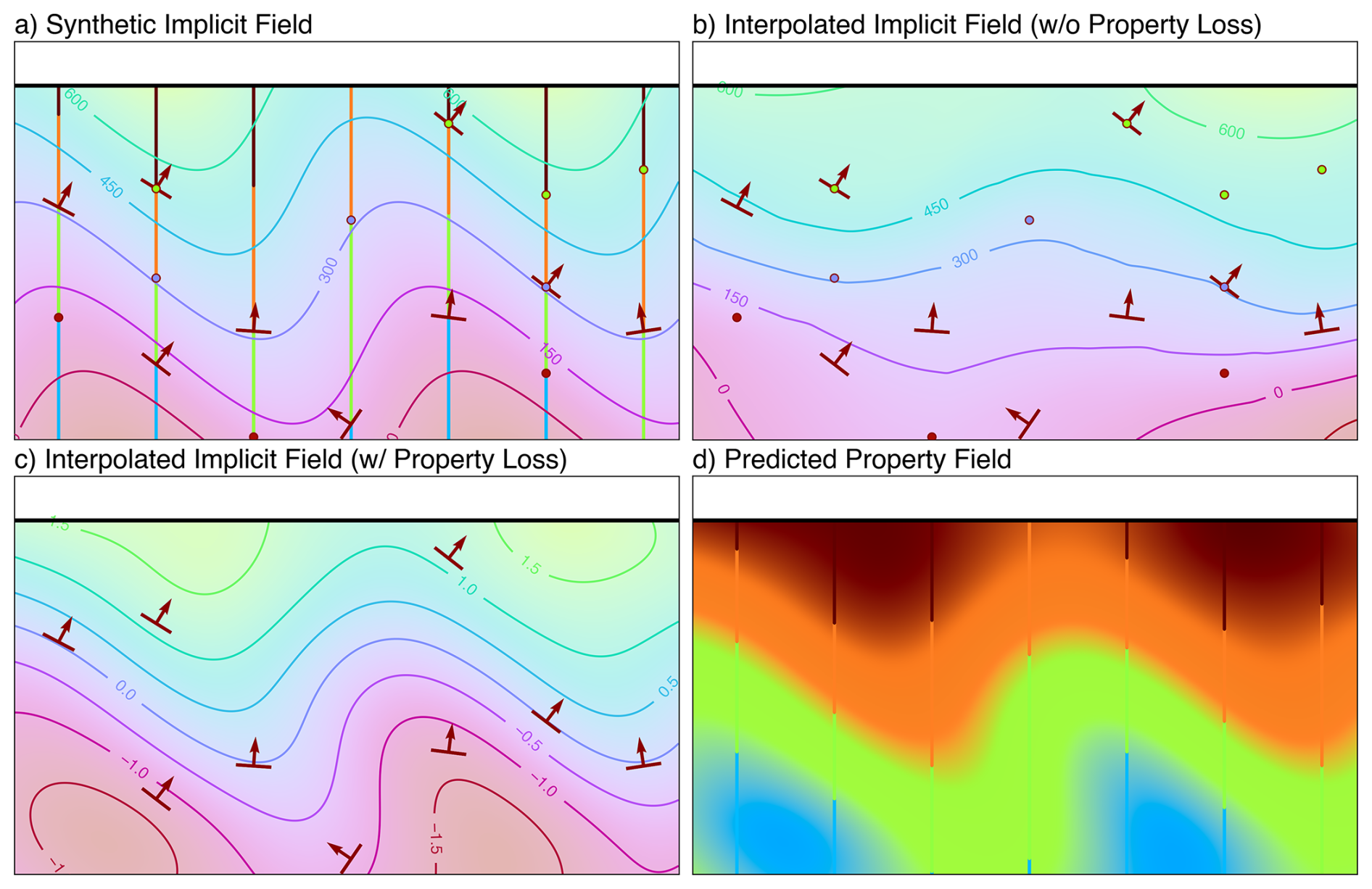
Figure 10 Synthetic (a) and interpolated implicit field derived without (b) and with (c) the learnable forward model. The original implicit field was sampled to extract sparse conventional (value and gradient) constraints and denser property measurements (coloured lines; analogous to geochemistry assays or hyperspectral drill core scans). The predicted model without the use of property constraints shows a wider folding in the basement due to lack of constraints. The addition of the learnable forward model allows the use of extra data, thereby tightening the wavelength of the interpolated model. The learnable forward model can also be evaluated across the entire domain (d) to show the recovered property field.

This approach potentially adds a powerful semi-supervised aspect to the modelling process: constraints are used to define an approximate (“supervised”) geometry, which is further refined to find solutions that best explains additional quantitative data or lithological logs, reducing interpretation bias and enabling the rapid integration of new data without explicit interpretation. A similar approach might also be used to integrate geophysical constraints on model geometry, albeit with physical forward models.

5.3 Future directions

The parameterisation of geological models using neural networks opens up several exciting directions for future research and application. The introduction of Random Fourier Features, while powerful, necessitates research into the extraction of appropriate length scales from sparse data, instead of the trial-and-error approach used in the current work. Progressive implicit representations (Landgraf et al., 2022) might also help in mitigating random noise generated by including high frequencies, while fitting sparse data better. Using the domain of the model and known sparsity of the constraints, one could also generate a power-spectrum of length scales to seed the model. This would effectively eliminate the need for a length scales hyperparameter. However, as the norms of the spatial wavenumbers follow a Chi distribution, the resulting distribution of wavenumbers includes a heavy tail. Careful optimisation is necessary to ensure that no spectral noise overtakes the interpolation process of the model.

We also note that our method of generating multiple model realisations by changing the Random Fourier Feature encoding has several similarities to the turning bands and spectral methods used to simulate Gaussian random fields (Mantoglou and Wilson, 1982), suggesting that a deeper stochastic link to other Gaussian process methods may be possible. The turning bands method uses the covariance matrix to seed the random field generation, which could possibly be adapted for the sparse datasets used as inputs to geological models. However, unlike the turning bands method, our method relies on Bochner's theorem (Bochner, 1955), which states that a shift invariant kernel i.e., the interpolator that the model is trying to approximate, is defined by the Fourier transform of the probability distribution of the frequencies used to construct the kernel. Using a uniform distribution (as suggested by Emery and Lantuéjoul, 2006, for turning bands simulations) signifies that the interpolator will behave as a Sinc- or Bessel-type kernel, and could cause ringing artifacts. A careful examination of alternative distributions for drawing these frequencies is also an avenue for future research.

The flexibility of the loss function used to train neural fields opens the door to additional innovative constraints that better encode geological rules or prior knowledge, e.g., topological relationships of the model outputs (Thiele et al., 2016a, b). However, incorporating multiple physical and geometric constraints further increases the complexity of our already complex multi-objective optimisation problem. Because different constraints often have entirely different numerical scales and physical units, each additional loss component requires careful hyperparameter tuning to prevent one objective from dominating the network's gradient updates.

To mitigate this in curlew, we implement an optional initial loss normalization strategy in which each individual loss component is divided by its detached initial value at the very start of training. This initial scaling forces all the losses to begin at 1, and can be thought of as an assumption that the losses at initialisation are equally bad. Once the losses are mapped to this common (unitless) scale, users can apply a single, intuitive scaling hyperparameter to explicitly dictate the relative physical or geological importance of one constraint over another. Our tests show that setting the local loss scaling hyperparameters to 1, and the global loss scaling hyperparameters between 0.01 and 0.1 serves as a good starting point for most models.

Alternative approaches, such as Gradient Surgery (Yu et al., 2020) and other gradient based algorithms (Zhang et al., 2024), exist to automatically select and adapt hyperparameters during training. However, further work is needed to assess the extent to which these are able to replace manual hyperparameter optimisation in the context of curlew. We have implemented one of these, SoftAdapt (Heydari et al., 2019), but with mixed results.

6 Conclusion

To conclude, we suggest that neural fields offer an exciting and flexible method for parameterising structural geological models, and hope that the lightweight, modular, open-source and well-documented software framework provided by curlew facilitates further development in this direction. While much work remains (cf. Sect. 5.3), we have applied curlew to real (Sect. 4.3) and structurally complex synthetic (Sect. 4.2) data to model geological structures that would challenge established approaches. Our novel loss function helps encode geological rules regarding lateral continuity (i.e. monotonicity loss), and extends earlier work by Hillier et al. (2023) to avoid assigning geological data arbitrary but restrictive values (value constraints, cf. Sect. 2.1), through our implementation of pairwise relational constraints. By chaining neural fields together, through overprinting and offsetting relationships, curlew is also able to represent a variety of geological structures (faults, dykes and domain boundaries) and incrementally build complex geological models. Our results indicate that the flexibility of neural fields, and their ability to incorporate geological rules and unlabelled categorical or quantitative geological data, make them a powerful tool for the next generation of structural geological models. We hope that curlew helps unlock some of this potential, and ultimately facilitates more accurate and less biased representations of the subsurface.