Assessing resolution sensitivity in coupled climate simulations with AWI-CM3

In this study, we evaluate the performance of the latest version of the Alfred Wegener Institute Climate Model, AWI-CM3, in two configurations at different resolutions, demonstrating that higher spatial resolution substantially enhances the model’s ability to reproduce key climate variables and processes. The medium-resolution configuration consistently reduces climatological biases compared to both the low-resolution setup and the CMIP6 (Coupled Model Intercomparison Project, phase 6) multi-model mean, particularly in polar regions and areas characterized by strong mesoscale dynamics. Improvements are especially notable in the simulation of sea ice variability, ocean circulation, and ocean-atmosphere interactions. The medium-resolution simulation also exhibits greater interannual variability, which may reflect a more realistic representation of underlying processes, but whose implications will need to be fully assessed with multiple ensemble members. We conclude that long-term, eddy-permitting climate projections offer promising avenues for reducing structural uncertainties in future climate projections. As global modeling efforts move toward CMIP7 and beyond, our results highlight the importance of pursuing medium-resolution strategies in parallel with improved physical parameterizations and ensemble-based evaluation to more robustly capture the nonlinearities of the Earth system.

1 Introduction

The continuous development of climate models across successive phases of the Coupled Model Intercomparison Project (CMIP) progressively enhances our ability to simulate Earth's climate. However, studies have also highlighted persistent limitations in the current generation of models (Tokarska et al., 2020), raising concerns about the accuracy and reliability of their projections (Roach et al., 2020; Chen et al., 2021; Eyring et al., 2021; Slingo et al., 2022; Heuzé and Liu, 2024). These concerns are particularly relevant for the polar regions, where small-scale processes play a crucial role in shaping large-scale ocean and atmospheric dynamics (Heuzé et al., 2013; Marshall and Speer, 2012; Hewitt et al., 2022). One of the key factors contributing to these limitations is the relatively coarse spatial resolution of current climate models (Bock et al., 2020; Rackow et al., 2022; Li et al., 2024). In phase 6 of CMIP (CMIP6), global climate models (GCMs) typically use horizontal grid spacings of 100–200 km (roughly 1°) in both atmosphere and ocean components (Eyring et al., 2016). At these resolutions, critical mesoscale and submesoscale processes, such as eddies and turbulent mixing, are not fully resolved and must be parameterized, which indirectly affects other processes, including boundary currents, and introduces uncertainties into climate simulations (Hallberg, 2013; Griffies et al., 2015).

In the Arctic, CMIP6 models have proven capable of simulating atmospheric conditions with reasonable accuracy (Song et al., 2021; Zapponini and Goessling, 2024), but exhibit biases in their representation of sea ice cover (Notz and SIMIP Community, 2020), sea ice-ocean interaction and ocean circulation (Muilwijk et al., 2024; Athanase et al., 2025), as well as deep ocean convection (Heuzé et al., 2023). Regional evaluations show that CMIP6 models are broadly capable of capturing large-scale temperature and precipitation patterns in tropical to mid-latitude regions (Mmame and Ngongondo, 2024; Taylor et al., 2023), but biases persist in the representation of extreme events (Rabezanahary et al., 2024; Zhang et al., 2025a) and regions with complex orography (Pimonsree et al., 2023), emphasizing the importance of selecting appropriate models for regional climate studies. Additional systematic biases include the misrepresentation of the mid- to high-latitude cloud phase, potentially impacting the Earth's energy budget (Hellmuth et al., 2025). In the Southern Ocean, CMIP6 models struggle to accurately capture long-term sea ice trends (Roach et al., 2020; Casagrande et al., 2023) and short-term variability events such as polynyas (Mohrmann et al., 2021). This is partially attributable to persistent biases in representing air-sea heat fluxes (Cesana et al., 2022, 2025). Similarly, the properties of the ocean water masses over the full depth remain poorly represented (Beadling et al., 2020). Taken together, these studies illustrate both the advances CMIP6 models have made over previous generations in simulating various high-latitude climate processes and the biases that remain, underscoring the need for model improvements, particularly for higher-resolution simulations capable of capturing small-scale processes and feedback mechanisms critical to polar climate dynamics.

Advancements in this direction have included the development of higher-resolution CMIP6 models, such as those in the HighResMIP protocol (Haarsma et al., 2016), where grid spacings are reduced to below 50 km in some cases. These simulations have demonstrated notable improvements in key aspects of climate representation, including ocean heat transport, atmospheric circulation, and sea ice distribution (Bock et al., 2020). More recently, coupled global simulations at kilometer-scale resolution (below 10 km) have become feasible, demonstrating striking improvements in the representation of mesoscale eddies and sea ice–ocean interactions (Hohenegger et al., 2023; Rackow et al., 2025; Moon et al., 2025; Doblas-Reyes et al., 2026).

However, while these higher-resolution models significantly reduce uncertainties associated with some parameterizations, their computational demands escalate rapidly with increasing resolution. Running models like this can require strategic partnerships, such as with the European High Performance Computing Joint Undertaking (EuroHPC) in the Destination Earth project (Doblas-Reyes et al., 2026). Global kilometer-scale ocean models can resolve mesoscale eddies across all latitudes and improve representations of the sea ice–ocean interface, including ice-shelf cavities. Their computational demand, however, generally limits them to decadal simulations, falling short of the timescales required for CMIP-class climate projections.

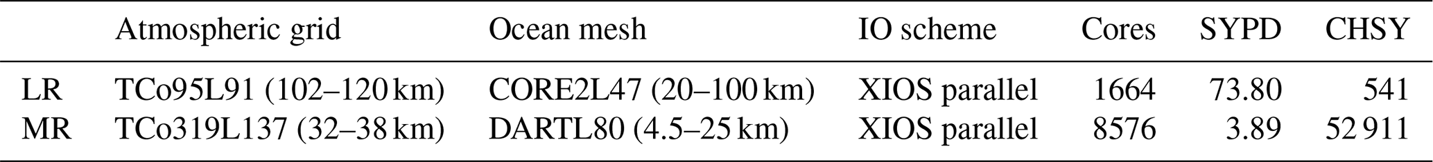
Here, we build on these developments by using the most recent version of the Alfred Wegener Institute (AWI) general circulation model, AWI-CM3 (Streffing et al., 2022), to perform fully coupled simulations spanning both the historical (1950–2014) and future (2015–2100) periods. We employ two distinct model configurations: a medium-resolution setup, MR (TCo319L137-DART) and a standard CMIP6-type low-resolution setup, LR (TCo95L91-CORE2). The nomenclature (e.g., TCo319L137-DART, TCo95L91-CORE2) reflects the horizontal and vertical resolution of the atmospheric component (spectral truncation TCo and vertical levels L) and the choice of ocean grid (DART or CORE2). The MR and LR experiments follow the CMIP6 HighResMIP protocol and include a 100-year spin-up to reduce model drift, ensuring comparability across resolutions.

The aim of this study is to assess how AWI-CM3’s performance varies with spatial resolution, focusing on the impact of finer grid spacing on key climate variables, simulation accuracy, and the representation of small-scale processes. In this respect, our work is best understood as a companion piece to both Streffing et al. (2022) and Moon et al. (2025). Streffing et al. (2022) presented the first prototype of the model version used in all simulations analyzed here, primarily focusing on the configuration referred to in this study as LR. We extend this work by evaluating AWI-CM3 performance at a significantly higher resolution. In contrast, Moon et al. (2025) compared the MR configuration against a computationally demanding high-resolution (HR) setup, providing valuable insights into the benefits of kilometer-scale climate modeling, but over relatively short simulation periods and with an emphasis on selected processes. Here, we broaden the scope of analysis by also examining the general characteristics of the large-scale ocean and atmospheric circulation. In addition, our study compares MR directly with CMIP6-standard LR, assessing its added value for widely used intercomparisons. While Moon et al. (2025) emphasize the potential of HR simulations, we show that regionally enhanced simulations at MR provide long-term, computationally affordable simulations covering the full historical period and continuous projections through 2100, improving climate projections while remaining feasible for multi-century CMIP-class experiments.

2 Model setup

AWI-CM3 is a coupled global climate model consisting of the OpenIFS cycle 43r3 atmosphere model (ECMWF, 2017a, b, c) and the FESOM2 sea ice-ocean model (Danilov et al., 2017). Included in the atmospheric component are the WAM module for waves (Komen et al., 1996) and the H-TESSEL module for hydrology (Balsamo et al., 2009). Coupled to it is the parallel XML Input/Output Server (XIOS) 2.5 (Yepes-Arbós et al., 2022). The ocean model incorporates the FESIM sea ice module (Danilov et al., 2015) which employs a modified elastic–viscous–plastic (EVP) rheology (Koldunov et al., 2019b). AWI-CM3 also features a river routing scheme, which processes land surface water balance from the atmosphere and directs runoff to coastal discharge points of the ocean, based on river basin maps. More detailed descriptions of the model components and coupling can be found in Streffing et al. (2022).

The model is run using two different configurations: a lower and a higher resolution, called respectively LR and MR (medium-resolution) in this paper. The atmosphere model operates at the cubic octahedral TCo95 and TCo319 horizontal resolutions, which correspond to a range of approximately 102–120 and 32–38 km from the equator to the poles, with respectively 91 and 137 vertical levels up to a top pressure level of 0.01 hPa. The ocean model uses an unstructured mesh approach with resolution varying depending on the ocean dynamics and latitude (Sein et al., 2017, Fig. 1). Here, the horizontal resolution of the CORE2 mesh ranges from 20 km in the Arctic, 40 km across the Southern Ocean, and 100 km in subtropical regions (about 127 000 surface nodes, Koldunov et al., 2019a), whereas the DART mesh achieves finer resolution, from 4.5 km in the Arctic, 10 km across the Southern Ocean, and 25 km in subtropical regions (3.1 million surface nodes). In the vertical, the former has 47 vertical levels while the latter has 80 vertical levels. A more detailed description of the two meshes is available in Streffing et al. (2022). In both cases FESOM2 was configured with the linear free surface vertical coordinate system, which allows the ocean surface to move up and down in response to external forcing. In all the simulations reported here no partial cell layer at the bottom has been enabled.

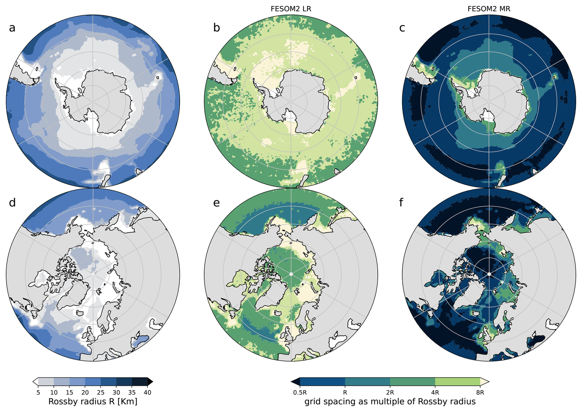
Figure 1 Local Rossby radius of deformation (a, d) estimated as $R=\left(\mathit{\pi }f{)}^{-\mathrm{1}}{\int }_{-H}^{\mathrm{0}}N\right(z)\mathrm{d}z$ where f is the Coriolis parameter, H is the ocean floor, and N is the Brunt-Väisälä frequency (as in Sein et al., 2016). Ocean horizontal grid spacing as a multiple of the local Rossby radius for the (b, e) low and (c, f) high resolution meshes (CORE2 and DART respectively). Blue (dark blue) colour marks the eddy-permitting (eddy-resolving) areas.

The atmospheric model operates at 3600/900 s time steps, while the ocean model runs at 1800/240 s time steps for LR and MR, respectively. The coupled configuration employs the OASIS3-MCT_4.0 coupler (Craig et al., 2017) with a 2 h/1 h coupling time step. In Table 1 we report the computational performance for the two simulations.

Table 1 AWI-CM3 computational performance in the two different configurations. Atmospheric grids and ocean meshes are listed together with their respective horizontal resolution ranges (in parentheses). The total number of cores used, the number of simulated years per day (SYPD) and the core hours per simulated year (CHSY) are reported for both configurations.

The LR mesh does not resolve or permit ocean eddies (Fig. 1b, e); the effect of mesoscale eddies on tracers is included employing the Gent–McWilliams (GM) parameterization (Gent and Mcwilliams, 1990). In contrast, the MR mesh is eddy-permitting across most of the domain – except for the southernmost part of the Southern Ocean and regions with complex topography – and is locally eddy-resolving (Fig. 1c, f). As a result, the GM parameterization is disabled throughout the entire domain. Following standard modeling practice, the Redi scheme (Redi, 1982), which typically accompanies GM to represent isopycnal tracer diffusion, is also deactivated. This setup allows us to evaluate the historical performance and analyze future projections of a simulation that permits mesoscale dynamics across most of the ACC core and the inner Arctic Ocean. In both cases, ocean vertical mixing is simulated through the K-profile parameterization (KPP) mixing scheme (Large et al., 1994), but in the MR configuration an additional vertical mixing within the Monin-Obukhov length scale (Timmermann and Beckmann, 2004) is enabled for the area south of 50° S to better represent vertical mixing under sea ice (Scholz et al., 2022).

2.1 Simulation protocol

As mentioned previously, both simulations were performed following the HighResMIP protocol, with an extension of the spin-up length to 100 years. A one-year coupled spin-up with a reduced ocean time step was performed beforehand exclusively for the MR configuration to mitigate initial shocks from the PHC3 ocean climatology initialization (PHC3.0, updated from Steele et al., 2001). From the final state of the spin-up, both a control simulation (ctl, 151 years) and a transient simulation (65 + 86 years) were initialized. During the spin-up and the control simulation, greenhouse gases and aerosol concentrations were fixed at 1950 levels. In contrast, the transient simulations followed the CMIP6 historical and SSP585 scenario forcings for greenhouse gases and aerosols (Meinshausen et al., 2017).

For both simulations, a single simulation has been performed and analyzed in this study. This is primarily due to the limitations with regard to available computing resources, which make the production of multiple ensemble members in the MR configuration challenging (Table 1). Further discussion of this aspect is provided in the Conclusions.

2.2 Model tuning

The two simulations were carried out using the same AWI-CM3 model version; however, as previously noted, the set of physical parameterizations applied varies with spatial resolution. The goal of this study is to evaluate the impact of resolution on model performance. To achieve this we have chosen to compare two simulations that are each optimized for their respective grid resolution. Parameter choices in both setups result from dedicated tuning processes designed to maximize performance at each resolution, which closely follows the approach of the HighResMip2 protocol for CMIP7 (Roberts et al., 2025). Differences in parameter settings were anyway kept to the minimum, to ensure as clear a comparison as possible, with only a small number of technical parameters adjusted during tuning. Among the tuned parameters, albedo usually plays a particularly influential role due to its strong effect on the model’s radiative balance and surface energy fluxes. In our model, distinct four constant albedo values are prescribed for sea ice, snow, and melting ice or snow. A common set of values was identified during the tuning process and applied consistently across both configurations.

It is worth noting that the simulation presented in this study is based on a slightly updated version of AWI-CM3 compared to the setup described in Moon et al. (2025), though the two remain highly comparable. The most significant difference concerns the remapping method used for ice-related heat fluxes exchanged between the atmosphere and ocean via the model coupler. In the earlier setup, the Gaussian remapping method introduced a spurious heat flux over ice-covered regions of the Northern Hemisphere leading to a reduced sea ice extent and premature disappearance of sea ice (Fig. A1). In this model version that has been replaced by a bi-cubic remapping method that improves the Arctic sea ice representation. The Southern Hemisphere was not affected by the previous issue, and we do not observe a substantial change in the simulation of Antarctic sea ice.

3 Results

3.1 Model drift and equilibration

Before evaluating the climatological performance of the simulations, we assess the degree of equilibration of the coupled system under constant forcing. While AWI-CM3-LR exhibits a clearly positive top-of-atmosphere (TOA) radiative imbalance since the beginning of the simulation, AWI-CM3-MR starts with near-zero values; both simulations, however, display a declining trend during the spin-up phase (Fig. 2a, b). After spin-up, the imbalance stabilizes at approximately +0.2 W m⁻² in the low-resolution configuration, reasonably on the lower of CMIP6 models average and reference estimates for the present-day climate (Johnson et al., 2016; Wild, 2020), and at a nearly symmetric negative value (∼ −0.24 W m⁻²) in the medium-resolution case. The surface energy imbalance is smaller in the LR simulation and more pronounced in the MR configuration, but in both cases it closely follows the evolution of the TOA flux. The relatively stable TOA–surface difference indicates that the atmospheric column remains internally consistent, while suggesting that, particularly in the MR simulation, the residual energy imbalance is primarily associated with ongoing ocean adjustment.

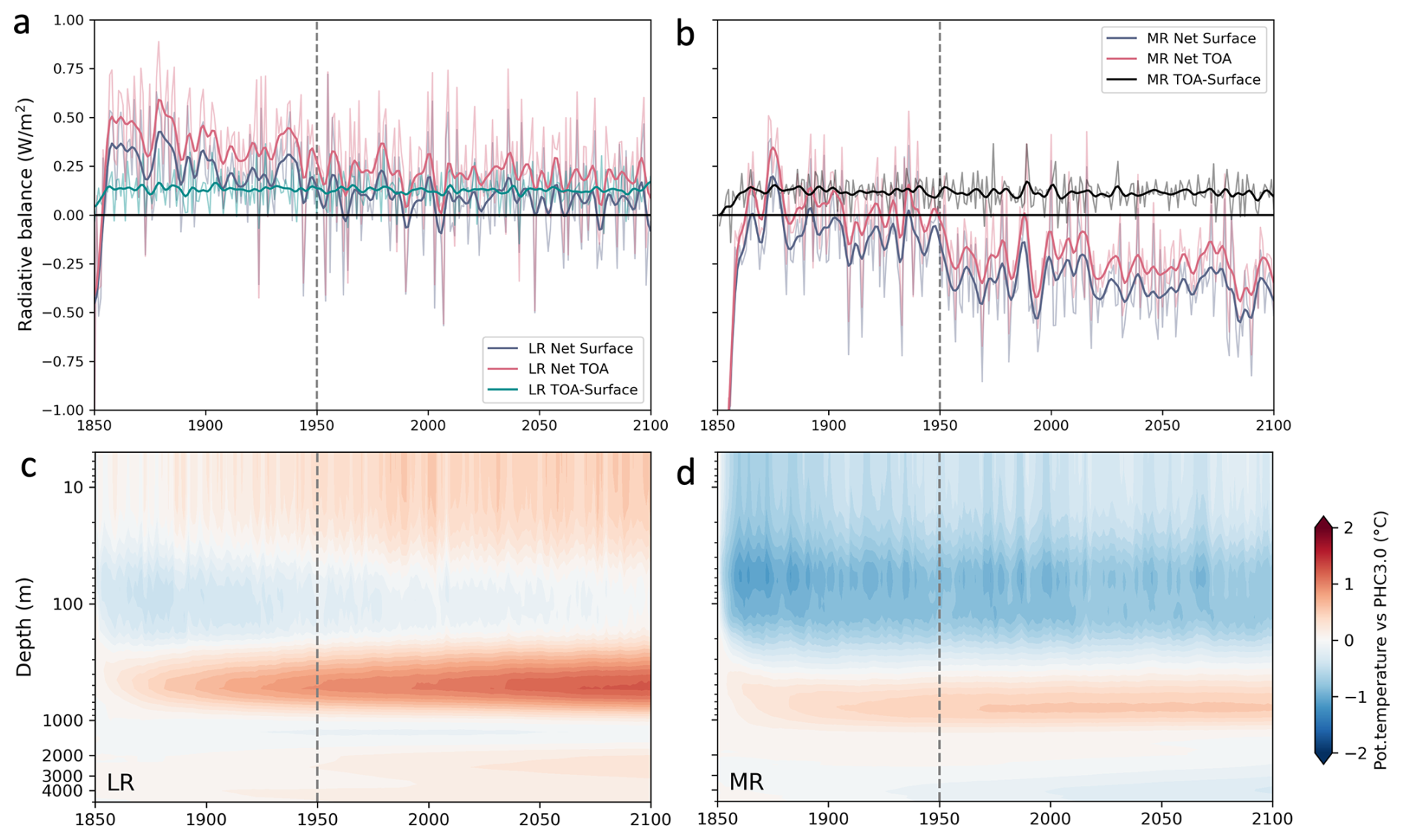
Figure 2 (a, b) Net radiative imbalance at the top of the atmosphere (TOA) and at the surface, together with their difference, representing the atmospheric column energy balance, during the spin-up and control simulations. Positive (negative) values indicate downward (upward) fluxes. (c, d) Hovmöller diagrams of the evolution of global-mean ocean potential temperature bias during the spin-up and control simulations, relative to the PHC3.0 climatology. The vertical dashed line marks the branch-off point of the transient simulations. Results are shown for the low-resolution (LR, left panels) and medium-resolution (MR, right panels) configurations.

In both configurations, the global-mean ocean temperature bias exhibits a relatively stable vertical structure (Fig. 2c, d). However, differences emerge in both the temporal evolution and the magnitude of these biases. In the LR simulation, a weak cold bias around 100 m is present during the initial adjustment phase and diminishes over time as warm biases at intermediate depths become more pronounced. This is accompanied by a persistent subsurface warming throughout the control period, indicating a sustained drift in the ocean interior despite the near-stationary behavior of the global energy budget, broadly consistent with Streffing et al. (2022). In contrast, the HR simulation shows a more stable depth-dependent pattern and less pronounced ocean temperature drift, with weaker subsurface warming and a clear upper-ocean cooling, consistent with a net upward energy flux at both the surface and the TOA.

While the low-resolution simulation can be considered reasonably equilibrated by 1950, the medium-resolution configuration still exhibits signs of residual imbalance at the time the transient simulations are branched off. This is reflected in the larger variability of the radiative balance and is consistent with the presence of an eddy-permitting ocean. Explicitly resolving mesoscale processes substantially increases the timescale required for the deep ocean to adjust (Danabasoglu et al., 1996). As a result, the approach to equilibrium is slower, and residual imbalances can persist over longer periods compared to lower-resolution configurations relying on parameterized processes (Danek et al., 2019).

Contrasts between low- and high-resolution configurations have been reported in HighResMIP and other multi-model studies, where increasing resolution leads to a reorganization, or even a reversal in sign, rather than a systematic reduction of model errors (Bock et al., 2020; Moreno-Chamarro et al., 2022). However, most relevant for the present comparison is that both simulations exhibit an overall limited and well-constrained drift from 1950 onwards. This is evident in the weak trends of global-mean sea surface temperature and near-surface air temperature, as well as in the relatively stable sea ice extent across seasons and regions (Fig. 4).

3.2 Historical climatology

To obtain an objective overview of the overall performance of the model, we use a multivariate comparison against observational climatologies. This approach provides a broad assessment of how well the model captures key climate features with respect to the CMIP6 multimodel ensemble. Eighteen key climate variables were selected for this evaluation. For each variable, we calculate the absolute climatological error in the AWI-CM3 simulations, considering all four seasons and seven distinct regions. The absolute error is first computed at each grid cell of an interpolated grid and is then averaged over each of the seven regions and over each season. Finally, the resulting model error is compared to the average absolute error of 30 CMIP6 models and expressed as a fraction of this CMIP6 mean error. Values below 1 indicate better performances, whereas values above 1 suggest larger errors (Fig. 3a). Only the last 25 years of the historical simulation (from December 1989 to November 2014, in line with the seasonal analysis) have been considered here to maximize comparability with the observational datasets. It is worth noting that not all observational datasets cover the entire period; a detailed overview of the coverage period for each variable is provided in Streffing et al. (2025). To directly compare the two simulations, the index for AWI-CM3-MR was computed again using AWI-CM3-LR as the simulation reference for the evaluation (Fig. 3b). In this way the MR simulations show better performances than the LR simulations for values below 1 and larger errors for values above 1.

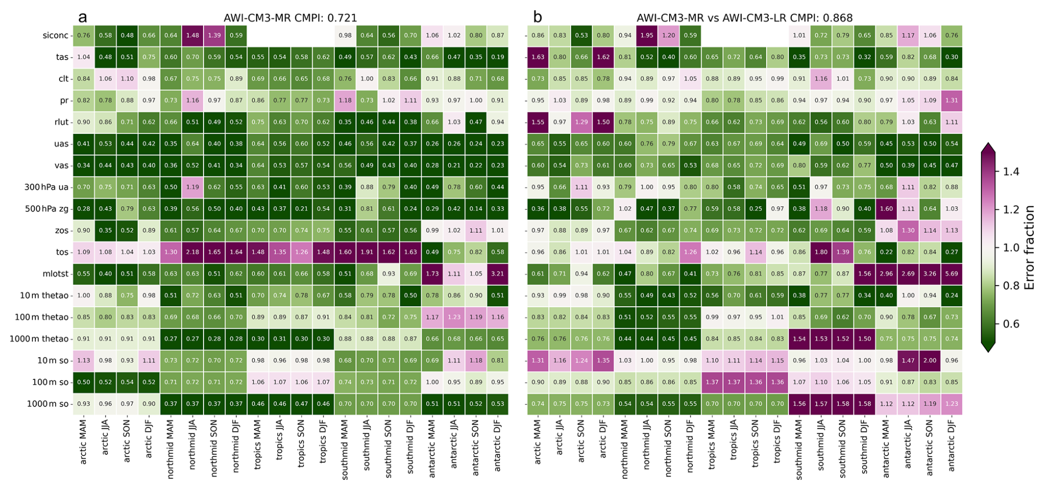
Figure 3 (a) Performance indices showing the absolute error of the AWI-CM3-MR historic climatology (1989–2014) expressed as a fraction of the CMIP6 multi-model mean absolute error (30 models; Streffing et al., 2025; Reichler and Kim, 2008). Values below (above) 1 indicate smaller (larger) biases compared to the CMIP6 average. Panel (a) compares AWI-CM3-MR against CMIP6, while Fig. A2 presents the same comparison for AWI-CM3-LR. (b) Performance indices comparing AWI-CM3-MR with AWI-CM3-LR, using the LR as reference. Here, values below (above) 1 indicate a reduction (increase) of error in MR relative to LR. The Arctic and Antarctic regions are defined as latitudes north of 60° N and south of 60° S, respectively; the mid-latitudes span 30–60° in both hemispheres; and the tropics cover 30° S–30° N. The list of all variables with full names is reported in Table A1.

The overall score, computed as the average across all variables, regions, and seasons, indicates a general improvement over the CMIP6 standard (Figs. 3a and A2) which, in the MR configuration (AWI-CM3-MR), corresponds to an average error reduction of 27.9 %. Examining the variable-specific errors, the simulation demonstrates a widespread reduction in the atmospheric absolute error relative to the CMIP6 models considered here, along with notable improvements in ocean dynamics. Large errors in sea surface temperature (tos) are primarily observed in the mid- and tropical latitudes and are associated with a persistent warm bias in the model (discussed in detail in Sect. 2.2), which is significantly reduced at higher latitudes, particularly in the Southern Hemisphere, when resolution is increased. It was previously noted that the model tends to display a substantial misrepresentation of mixed-layer depth (mlotst) in the Antarctic (Streffing et al., 2022), however in this case it is only in the MR configuration showing this error. Despite the larger error magnitude with respect to the LR configuration, the MR setup produces more realistic sea ice concentration (siconc) values in the region in austral summer and autumn, but shows less agreement with observations in winter and spring. In this case, the comparison among simulations is complicated by the notably higher variability of the MR simulation during the analysis period. In the Northern Hemisphere, sea ice concentration performs well across all seasons, except for an overestimated summer sea ice extent at mid-latitudes (discussed in details in Sect. 2.3), an error that is most pronounced in the MR simulation. The 2 m temperature is generally well-simulated, here the increased resolution leads to more substantial improvements in the Antarctic compared to the Arctic. Higher spatial resolution also has a broadly positive impact on surface winds (uas and vas, representing the zonal and meridional components respectively) at the global scale. Similar improvements are observed for the 300 hPa zonal wind (ua), the 500 hPa geopotential height (zg), and the top-of-atmosphere outgoing longwave radiation (rlut). Precipitation (pr) is improved primarily in the tropics, while enhancements in cloud coverage (clt) are most evident at high latitudes. Ocean temperature and salinity (thetao and so) are, on average, well simulated; however, the impact of increased resolution is not uniform across regions or ocean depths. The higher resolution in MR generally helps reduce the ocean warm bias, except in southern mid-latitudes at 1000 m depth, where the MR is warmer (Fig. A3a–d). On the other hand the salinity bias, which is still below average in the LR simulation (Fig. A2), is amplified at the surface, in the tropical upper ocean and in the Southern Ocean at 1000 m depth (Fig. A3e–h).

The overall evaluation scores show that the LR simulation achieves a ∼ 13 % error reduction relative to the CMIP6 multi-model mean, while the MR simulation improves this further to a ∼ 28 % reduction. Therefore, approximately 55 % of the total error reduction compared to the CMIP6 standard can be attributed to the increase in spatial resolution. While this overall score provides a useful summary of model performance, it involves an inherent degree of arbitrariness, as it depends on the selection of variables and regions. It is therefore interpreted alongside the individual diagnostics presented below, rather than as a standalone measure of model skill. In the following, a more detailed analysis is conducted to assess specific aspects of the two simulations.

3.3 Surface temperature

A visible difference between the two model configurations lies in their mean state temperature bias. Even in the control simulation, a persistent offset is evident: the LR configuration is, on global average, approximately 1.5 °C warmer than the MR configuration for both sea surface and near-surface air temperatures (Fig. 4a). A similar bias is also evident in the transient low-resolution simulation when compared to observations, becoming particularly pronounced from the last decade of the 20th century onward. In contrast, the MR setup more closely reproduces the observed magnitude of the global mean surface temperature. During most of the satellite era (1990 onward), the MR configuration better represents the observed near-surface air temperature trend (MR: 0.25 °C per decade; LR: 0.19 °C per decade; ERA5: 0.24 °C per decade).

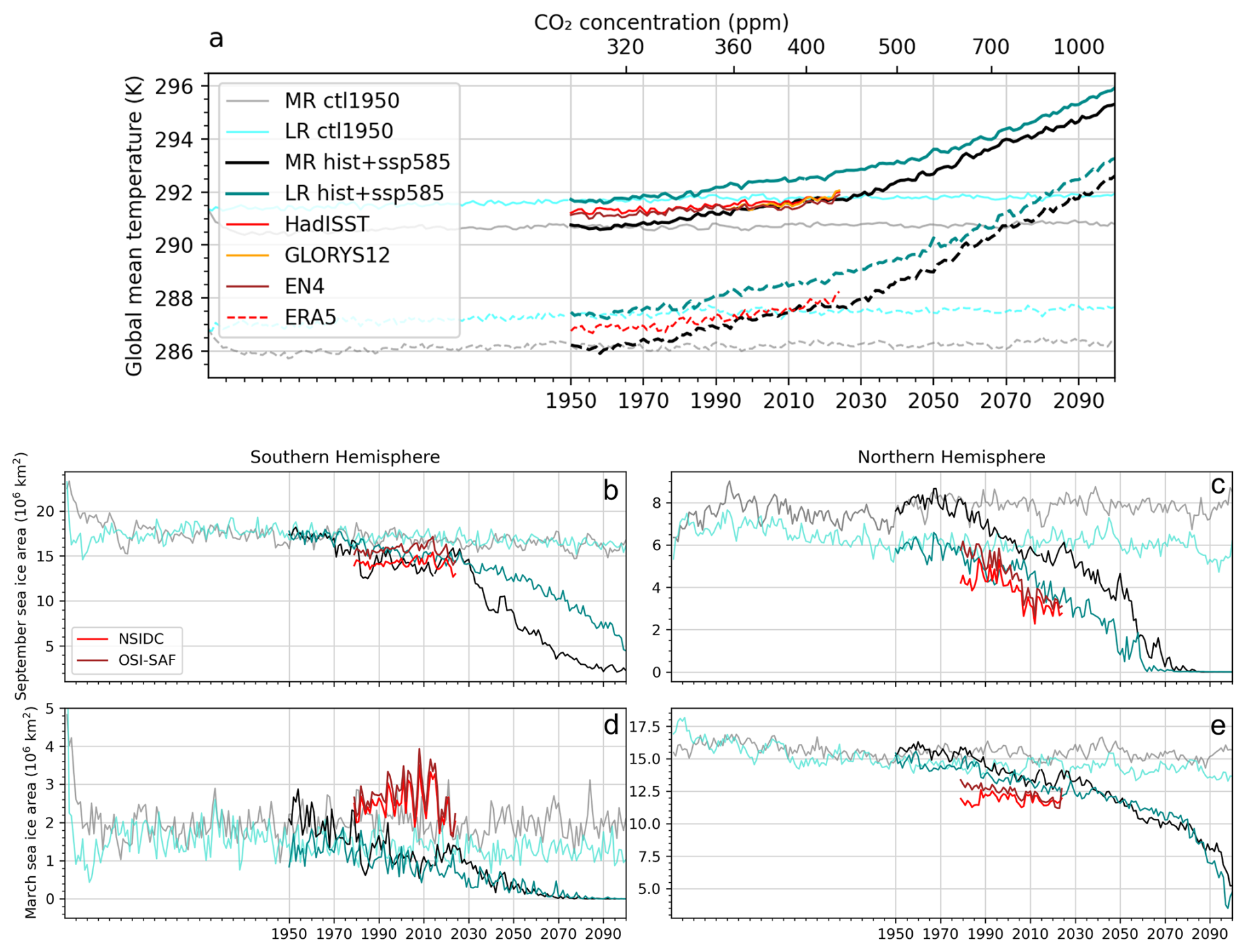
Figure 4 Time series of (a) global mean sea surface (full line) and 2 m air (dashed line) temperatures and (b–e) sea ice extent for the two hemispheres. Temperature is reported as annual mean, while for sea ice September and March means are represented separately. Light/dark green represent the low resolution experiment (LR) and gray/black lines represent the medium resolution experiment (MR). Light green and gray show the control runs while dark green and black show the hist+ssp experiments. Due to observational uncertainty, especially when looking at polar regions, multiple datasets have been included for observed sea surface temperature, 2 m air temperature, and sea ice area: HadISST1 (Rayner et al., 2003), GLORYS12 (Lellouche et al., 2021), EN4 (Good et al., 2013), ERA5 (Bell et al., 2021), NSIDC (DiGirolamo et al., 2017) and OSI-SAF (Lavergne and Down, 2023).

For sea surface temperature, both simulations exhibit a warming trend stronger than observed, with the MR configuration showing the largest deviation (MR: 0.18 °C per decade; LR: 0.14 °C per decade; HadISST: 0.11 °C per decade). It is also worth noting that the low-resolution simulation exhibits a stronger residual model drift in its control experiment, which is substantially mitigated by increasing the spatial resolution, consistent with the suggestion of Griffies et al. (2015), who highlight the role of numerical methods and physical parameterizations in contributing to model drift. Over the 151-year simulations, the total surface temperature drift in the LR configuration amounts to 0.21 °C in the ocean and 0.24 °C in the atmosphere, compared to only 0.06 and 0.10 °C in the MR configuration, respectively.

The spatial distribution of the biases highlights how the surface warm bias in the lower-resolution setup is fairly homogeneous at the global scale, affecting both atmosphere and ocean (Fig. 5a, i). Nonetheless, specific hot spots emerge – such as the El Niño/La Niña upwelling regions, the Southern Ocean, and the so-called northwest corner of the North Atlantic Ocean, identified as common biases in GCMs (Sein et al., 2017; Bock et al., 2020; Streffing et al., 2022) and references therein) – as well as the Kuroshio region. Consistent with comparisons between CMIP6 and HighResMIP (Bock et al., 2020), the magnitude of these biases is significantly reduced when horizontal resolution is increased (Figs. 5e, m and A4). The negative surface temperature bias near the equator, previously identified in the AWI-CM3 prototype (Streffing et al., 2022), is relatively weak in this LR simulation and is mostly confined to land areas. Conversely, much of the low- to mid-latitude region exhibits a cold bias in the higher-resolution configuration. The 2 m temperature bias over the central Arctic can to a large degree be explained by a warm bias present in the ERA5 reanalysis (Tian et al., 2024). At higher resolution, this negative bias exceeds 4 °C and peaks in the Canadian sector of the Arctic Ocean, while it is less pronounced at lower resolution. This pattern also resembles results obtained from comparisons of CMIP6 and HighResMIP multi-model means (Bock et al., 2020). However, as mentioned above, this difference must be contextualized, as recent studies indicate that ERA5 itself exhibits a warm bias exceeding 3 °C in the same region when compared with satellite observations (Tian et al., 2024).

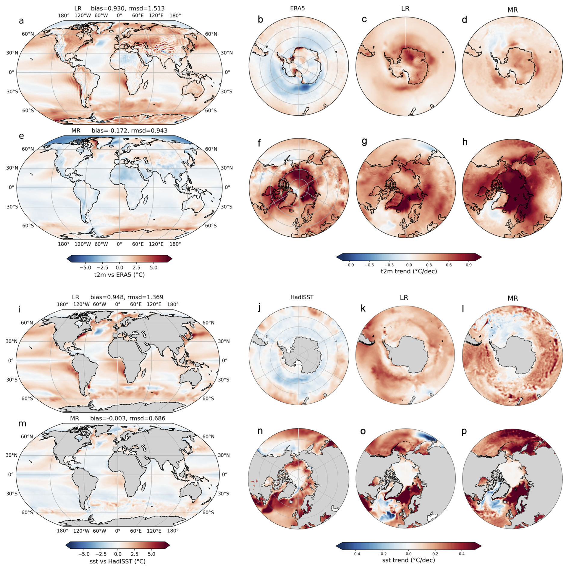
Figure 5 Annual mean (a, e) 2 m air temperature and (i, m) sea surface temperature biases for the period 1979–2014 relative to ERA5 and HadISST, respectively. Bias and rmsd represent the area-weighted mean and root mean square difference between model and observations. Annual mean 2 m air temperature (b–d, f–h) and sea surface temperature (j–l, n–p) trends over the same period, separately for the Northern and Southern extratropics (regions poleward of 40° N and 40° S), for both observations and model simulations. Results are shown for both the low-resolution (LR) and medium-resolution (MR) experiments.

The analysis of the last 35 years of the historical simulations indicates that the MR experiment exhibits a substantially reduced mean temperature bias, decreasing from 0.85 to –0.24 °C for global 2 m air temperature, and from 0.88 to –0.05 °C for sea surface temperature. Moreover, the observed global warming trend during this period is well reproduced in the MR simulation. Examining regional trends in the extratropics (Fig. 5b–d, f–h, j–l, n–p), the benefits of increased resolution are still generally evident, though in some regions less pronounced. In the Southern Hemisphere, the LR simulation fails to capture the observed cooling trend, instead displaying widespread warming in both the atmosphere and ocean (Fig. 5c, k). The MR simulation, by contrast, introduces more spatial detail: coastal regions tend to show weaker positive or neutral trends, and localized cooling, especially in the Pacific sector, is better represented (Fig. 5d, l). In the Northern Hemisphere, the MR simulation produces an overly strong surface air warming trend-especially pronounced at mid-latitudes-when compared to reanalysis data, likely related to the more pronounced cold bias (Fig. 5h). Meanwhile, the LR experiment shows only modest warming across much of the Arctic Ocean, with stronger trends confined to the Greenland and Barents Seas (Fig. 5g). For sea surface temperatures, both simulations reveal broadly similar warming patterns in the Northern Hemisphere extratropics; the erroneous negative trend in the Labrador Sea is here more clearly visible (Fig. 5o, p), especially in the MR simulations. Overall, while the MR simulation significantly reduces global mean temperature biases and better captures regional details, especially in the Southern Hemisphere, its improvements in replicating observed spatial trend patterns remain limited and regionally dependent for this individual realization. It is worth noting that regional trend patterns can be strongly affected by internal variability and part of the mismatch with observations may reflect this variability rather than systematic model biases.

3.4 Sea ice and mixed layer depth

The medium-resolution configuration exhibits a stronger increase in air temperature per unit of CO₂ concentration already during the historical period, with this difference becoming even more pronounced starting from the late 2020s (Fig. 4a). A similar, though slightly less pronounced, signal is also evident in the sea surface temperature. It is noteworthy that this year also marks the onset of a pronounced regime shift in the maximum sea ice area over the Southern Ocean (Fig. 4b): within approximately 15 years, Antarctic sea ice loses nearly 7 million km² of its area. This rapid decline is analyzed in detail by Kim et al. (2026). Here, we simply note that such a sharp decline is absent in the low-resolution simulation, which instead shows a more gradual and stable decrease typical of many CMIP6 models. Enhanced sea ice variability in the Southern Ocean is also apparent prior to this event in the medium-resolution simulation, with several fluctuations linked to more or less severe Weddell Sea polynya episodes. For this reason, despite being an average over a long period of 25 years, the error displayed when computing the performance index (Fig. 3a) is influenced by this strong variability.

Several studies have shown that CMIP6 climate models tend to simulate a stably stratified Southern Ocean (Mohrmann et al., 2021). Consistent with this, the low-resolution AWI-CM3 simulation exhibits a shallow winter mixed layer depth (MLD) with very limited variability across most of the region south of 60° S (Fig. 6a, c). Notably, the Weddell Sea lacks any significant deep MLD features, showing some deepening only in a narrow coastal region. This behavior aligns with the limited polynya features in this model configuration. In contrast, the medium-resolution AWI-CM3 simulation shows pronounced MLD variations (Fig. 6b, d). Along the Antarctic coast, the MLD exceeds 200 m, consistent with active coastal polynya formation. In the Weddell Sea, the MLD reaches depths greater than 300 m, making it the region with the strongest variability in the Southern Ocean. This deeper and more variable MLD contributes to a more plausible representation of polynya occurrence, while at the same time leading to an overestimation of event intensity. It is important to note, however, that the observational record of polynya events is very limited, which adds uncertainty to such evaluations. The overly deep mixed layer is co-located with a localized and pronounced warm bias in 2 m air temperature (Fig. 5e), likely linked to enhanced oceanic heat release in this region. In contrast, the low-resolution configuration shows no such localized warm bias, instead displaying a relatively uniform positive bias across the Southern Ocean.

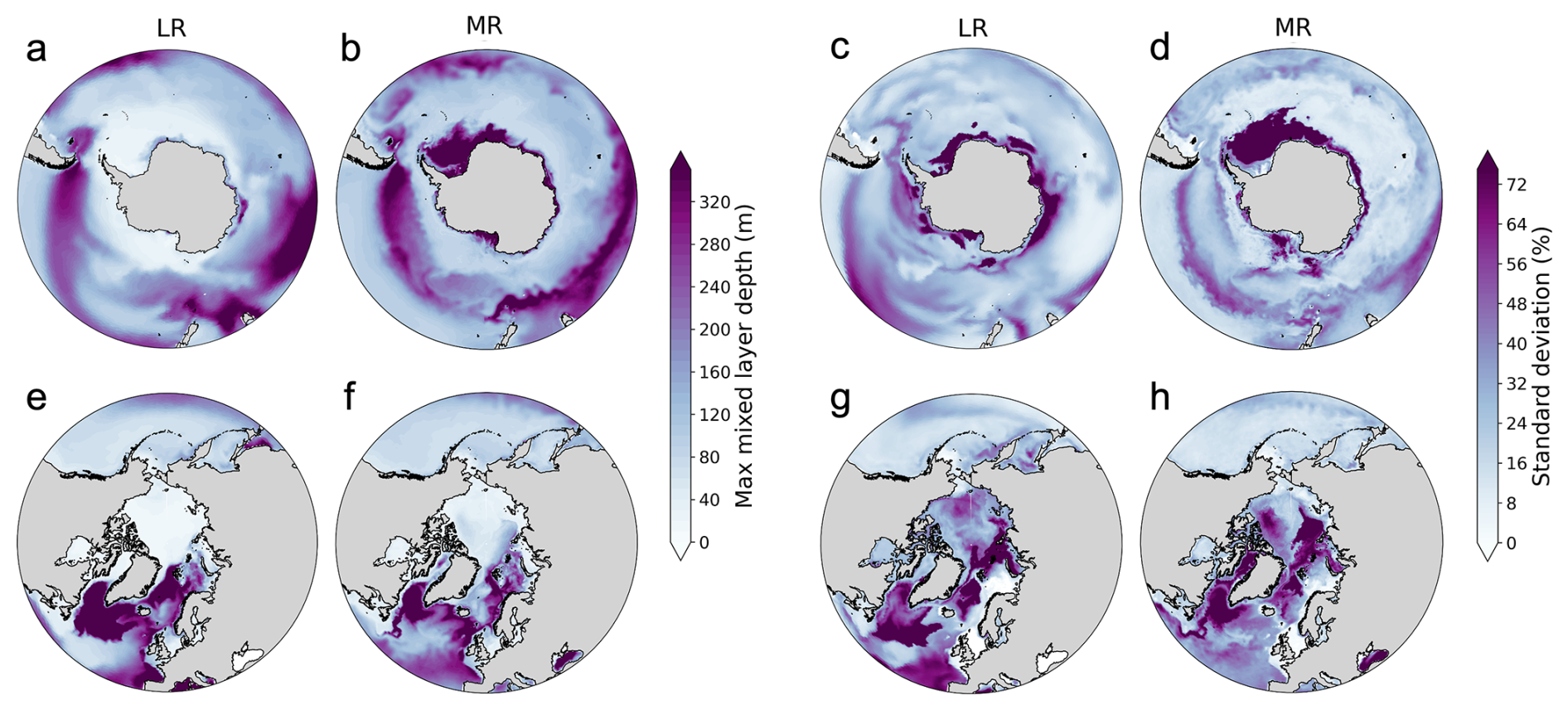
Figure 6 1979–2014 maximum winter mixed layer depth (a, b, e, f) and standard deviation (c, d, g, h) for the low resolution (LR, a, e, c, g) and medium resolution (MR, b, f, d, h) simulations. Respectively austral/boreal (JJA/DJF) winter season have been considered for the Southern/Northern hemisphere. MLD is defined as the depth at which the potential density differs by 0.03 kg m⁻³ from the surface density (Monterey and Levitus, 1997).

This discrepancy explains why the medium-resolution simulation exhibits greater variability in the inner Weddell Sea sea ice maximum compared to observations (Fig. 7a, e). Modeled September sea ice concentration trends in the Southern Hemisphere mirror the corresponding temperature trends (Figs. 5 and 7c, e): while the low-resolution simulation shows a largely uniform decline, the medium-resolution experiment captures some localized increases, such as in the Ross Sea and the Weddell Sea. However, both simulations display a marked retreat in sea ice concentration across East Antarctica, an inconsistency with satellite observations. In the Northern Hemisphere, the observed boreal summer sea ice loss in the central Arctic is largely absent in the low-resolution run but is reproduced, albeit with regional biases, at higher resolution, including excessive retreat in the Greenland and Barents Seas and an absent response in the Russian-Canadian sector (Fig. 7g, i, k). In March, sea ice extent is overestimated in the medium-resolution simulation (Fig. A5l) and shows indeed a more spatially distributed decline, stronger particularly at mid-latitudes (Fig. 7l), consistent with stronger positive temperature trends. In contrast, the low-resolution simulation exhibits spatial variability that more closely aligns with satellite data (Fig. 7i). During austral summer, neither simulation successfully reproduces the observed sea ice trends of the Southern Hemisphere (Figs. 7b, d, f and A5b, d, f). Overall, the main improvement associated with reduced grid spacing is a better representation of average sea ice trends (Fig. 4) and an enhanced ability to capture regional variability in the Southern Hemisphere. However, both resolutions still fall short in reproducing key observed features, such as the stability of East Antarctic sea ice and the full extent of Arctic summer sea ice loss.

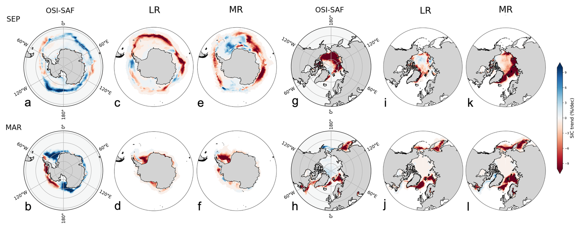
Figure 7 Trends in March and September sea ice concentration from 1979 to 2014 are shown for both hemispheres, based on OSI-SAF observations (a, b, g, h) and simulations from the low-resolution (LR, c, d, i, j) and medium-resolution (MR, e, f, k, l) model configurations. Although the two observational datasets display some differences in the time series shown in Fig. 4b–e, their spatial patterns of sea ice trends are largely consistent. The decision to present only OSI-SAF data here is motivated by its treatment of the central Arctic, where the typical data gap has been filled through interpolation.

3.5 Ocean circulation

The AWI-CM3 simulations reproduce the expected structure of the AMOC streamfunction in its mean state (Fig. 8a, b). However, two main differences emerge when comparing the streamfunctions from the low- and medium-resolution simulations. In the upper cell, within the 500–1500 m depth range, the low-resolution simulation shows a peak in northward transport primarily between 30 and 40° N, whereas the medium-resolution simulation displays a more uniform maximum across the latitudes. The comparison with observations at 26° N reveals that the medium-resolution simulation aligns more closely with the RAPID profile in the upper ocean but tends to overestimate the southward branch of the AMOC, suggesting a too-strong return flow of North Atlantic Deep Water (NADW) along the Deep Western Boundary Current (DWBC) (Fig. 8c, d). Conversely, the low-resolution simulation, while better capturing the magnitude of the NADW transport, locate its flow too shallow compared to observations (Fig. 8c, d), consistent with findings by Gutjahr et al. (2019), and with a too pronounced variability. Additionally, the medium-resolution simulation shows a clearer signal of northward transport of Antarctic Bottom Water (AABW) at abyssal depths (Fig. 8a, b). Similar resolution-dependent differences have been reported in earlier studies (e.g., Li et al., 2022).

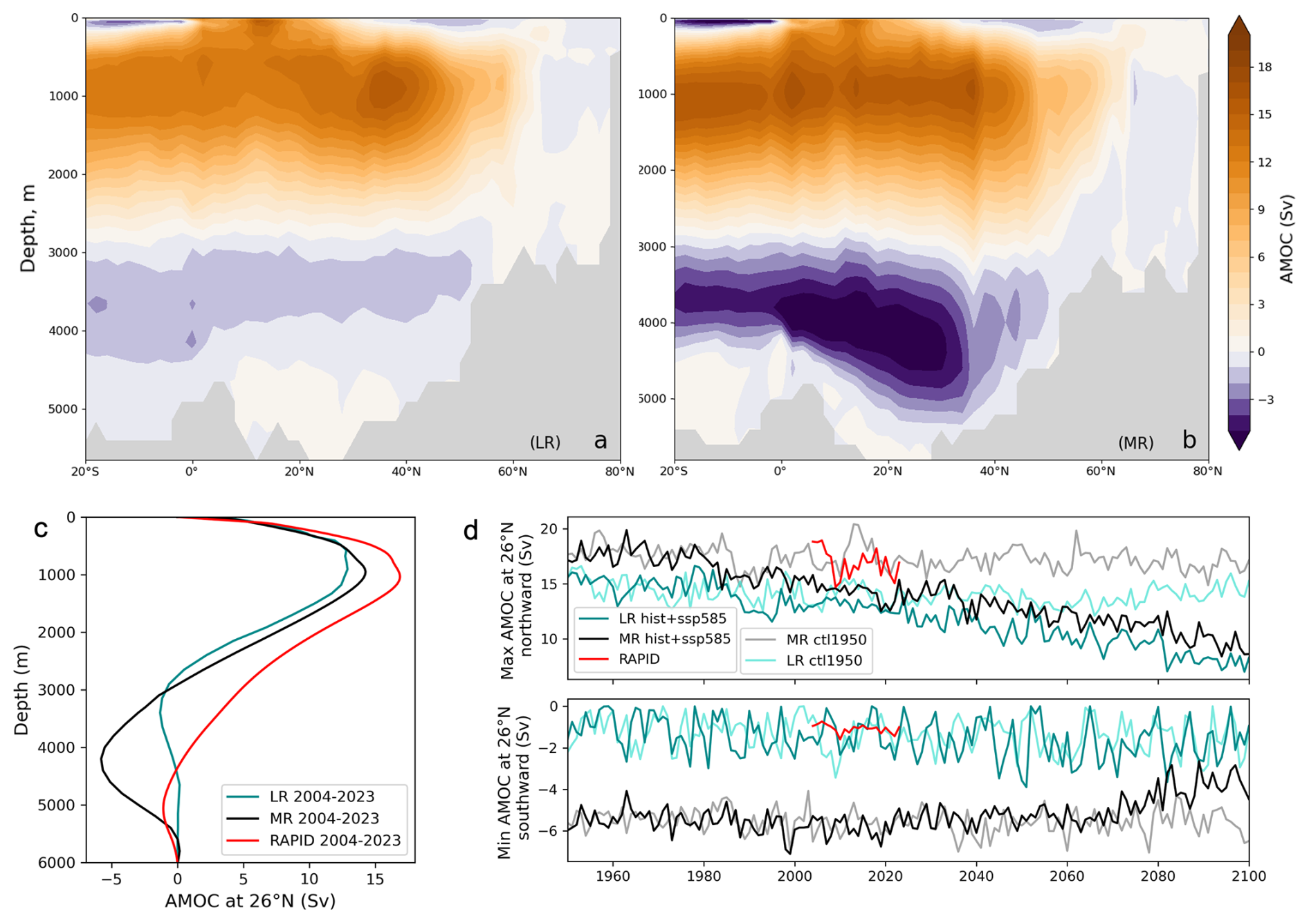
Figure 8 Atlantic Meridional Overturning Circulation (AMOC) overturning streamfunction averaged over the period 1979–2014 for (a) the low-resolution simulation (LR) and (b) the medium-resolution simulation (MR). (c) Comparison of AMOC overturning streamfunctions from AWI-CM3 simulations and RAPID-MOC array (Moat et al., 2024) observations at 26.5° N, averaged over the period 2004–2023. (d) Time evolution of AMOC maximum (northward transport) and minimum (southward transport) at 26.5° N from AWI-CM3 simulations and RAPID observations. (Sv denotes Sverdrups; 1 Sv = 106 m³ s⁻¹).

Starting around 1980, both simulations show a decline in the AMOC at 26.5° N under increasing atmospheric forcings (trend absent in the control simulations), but this weakening is confined to the northward flow component of the upper cell. In contrast, the southward branch exhibits no clear trend in the low resolution simulation, indicating a deep ocean circulation that is less sensitive to surface-driven changes, at least initially during the transient response phase. On the other hand, higher resolution shows more coherent changes between northward and southward transport, showing a decline in DWBC especially pronounced in the last two decades of the 21st century. As shown in Putrasahan et al. (2019), improving atmospheric resolution can lead to significant AMOC weakening via salinity-driven suppression of deep convection in the North Atlantic deriving from altered wind and ocean circulation.

Comparing the simulated volume transport across major ocean channels with observational estimates, provides initial insight into the effects of both increased horizontal resolution and a finer vertical discretization on ocean circulation and vertical processes (Table 2). In the Arctic, the medium-resolution simulation generally produces stronger volume transports across key straits compared to the low-resolution setup, with a tendency toward a positive bias relative to observations. Through the Davis and Fram Straits, the medium-resolution simulation falls within the observational uncertainty range, while the low-resolution one tends to underestimate the outflow. In contrast, the medium-resolution simulation overestimates poleward transports through the Barents and Bering Seas, leading to an excessive inflow of warm Atlantic and Pacific waters. This increased inflow likely contributes to a positive near-surface salinity bias in the Arctic Ocean, which is more pronounced in the medium-resolution case (Fig. 9a–d). This bias is consistent with known shortcomings of AOGCMs, often attributed to an insufficient freshwater supply from Siberian rivers (Gutjahr et al., 2019). At the same time, the enhanced northward transport in the medium-resolution simulation slightly reduces the warm bias (Fig. 5a, e) and significantly decreases the salinity bias in the North Atlantic near-surface (Fig. 9a, b).

(Curry et al., 2014)(Beszczynska-Möller et al., 2015)(De Boer et al., 2018)(Woodgate et al., 2005)(Woodgate, 2018)(Soto-Navarro et al., 2010)(Gordon et al., 2010)(Ridderinkhof et al., 2010)(Meredith et al., 2011)(Donohue et al., 2016)

Table 2 Mean ocean volume transport through selected straits and channels as simulated by AWI-CM3 in both configurations, compared with observational estimates (positive means northward or eastward). Model values represent averages over the period 1990–2014 of the historical simulation. References correspond to observational studies cited for each strait. (Sv denotes Sverdrups; 1 Sv = 10⁶ m³ s⁻¹).

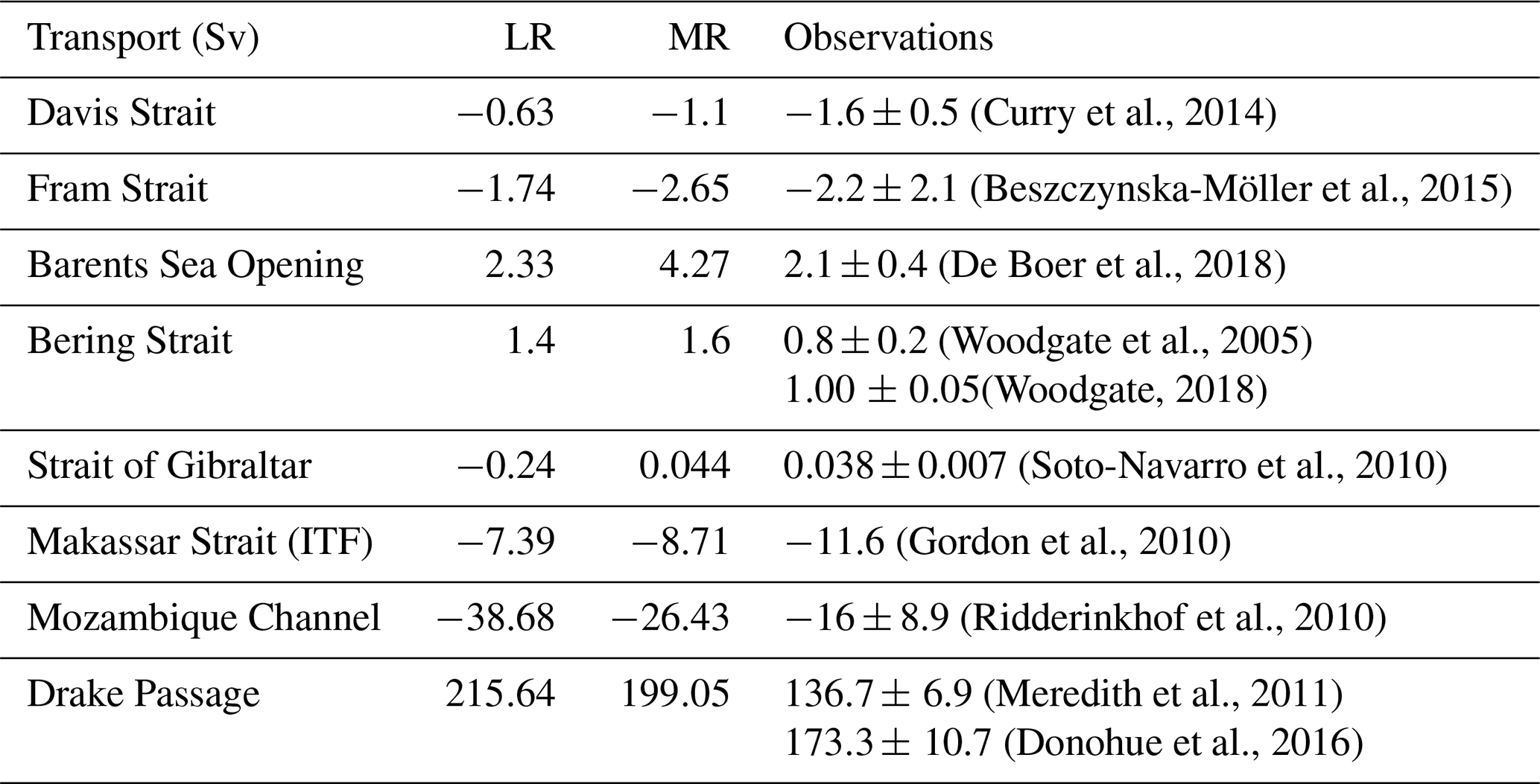
Improvements are also evident in the representation of the Gulf Stream separation, which reduces the localized fresh bias in the North Atlantic surface, and in the freshening of the Mediterranean Sea, which mitigates the excessive outflow of overly salty and warm Mediterranean waters around 40° N (Fig. 9c–f), present in the LR. These Mediterranean waters, in the low-resolution simulation, spread northward along the European continental shelf, contributing to a saltier and warmer NADW, which is then transported southward. The medium-resolution simulation shows improvements in ocean circulation and mixing processes, leading to a more realistic representation of deep water formation and large-scale circulation in the North Atlantic Ocean, consistent with the findings of Rackow et al. (2019).

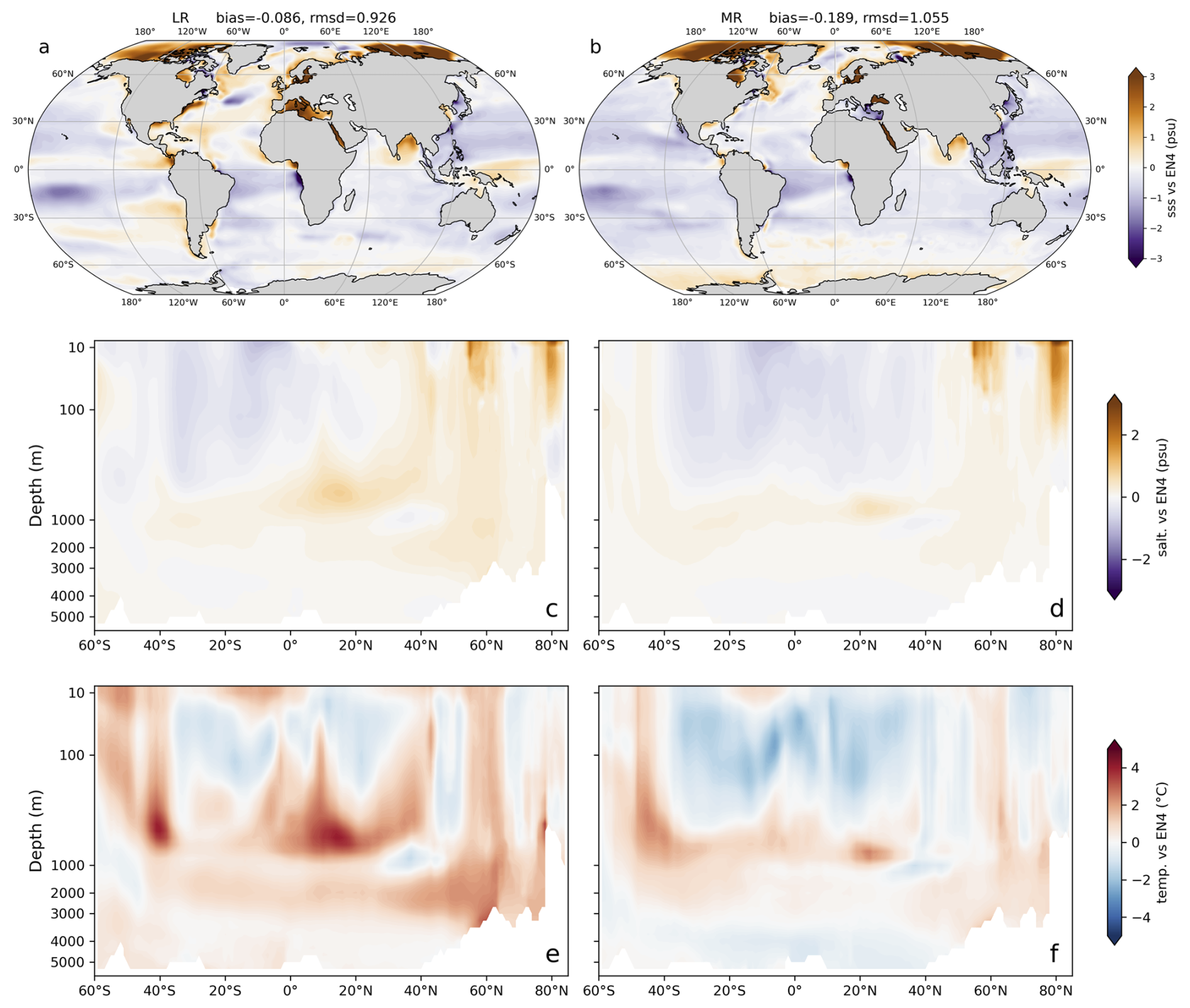
Figure 9 (a, b) Sea surface salinity mean bias and zonal mean (c, d) salinity and (e, f) temperature biases through the Atlantic Ocean and Arctic Ocean with respect to EN4. The biases, relative to the period 1979–2014, are shown for the low resolution (LR, left panels) and medium resolution (MR, right panels) simulations.

Consistent with Griffies et al. (2015), resolving mesoscale eddies in the medium-resolution simulation reduces the positive deep-ocean temperature bias overall, indicating more efficient vertical heat transport from the interior-with the exception of 1000 m depth where MR shows a slightly warmer bias than LR simulation in the mid-latitudes of the Southern Hemisphere (Fig. A3c, d). However, the surface ocean change from LR to MR is different from the classical eddy-heating effect in Griffies et al. (2015), where SST tends to warm when explicitly resolving mesoscale eddies. This pattern suggests that, while mesoscale processes improve deep-ocean realism, their effect on subsurface and surface temperatures is spatially heterogeneous, likely reflecting regional feedbacks such as stratification, sea ice dynamics, and coupled ocean-atmosphere interactions.

At higher southern latitudes, both model configurations tend to overestimate volume transports through the selected channels (Table 2). However, the medium-resolution simulation generally falls closer to the observational uncertainty ranges. A clear example is the transport through the Drake Passage, where both simulations produce a stronger Antarctic Circumpolar Current (ACC) than older observational estimates (e.g., Meredith et al., 2011). More recent full-depth measurements that include both baroclinic and barotropic components of the flow, however, indicate higher transport values (Donohue et al., 2016). In this context, the AWI-CM3 medium-resolution configuration approaches the upper bound of these updated observational estimates.

A well-known bias in low-resolution models is the incorrect representation of the Agulhas Current system. AWI-CM3 displays a similar feature, with an overly strong advection of warm waters from the Indian Ocean into the Atlantic at around 40° S (Fig. A3a, b). This bias then extends northward at Atlantic Intermediate Water (AIW) depths (Fig. 9c–f). Consistent with previous studies (Gutjahr et al., 2019; von Storch et al., 2016), resolving ocean mesoscale eddies leads to a more realistic ocean vertical stratification. In line with this, the medium-resolution simulation shows a reduction in the Agulhas leakage and in the warm and salty biases near the thermocline, particularly in subtropical regions, due to improved eddy-driven mixing (Fig. 9c–f). The only exception to that is a slightly increased salinity bias in the water column above 2000 m, between 40 and 60° S, but is part of the Brazilian current rather than of the Agulhas one.

It has been shown that variations in the Agulhas system can influence thermohaline properties in the North Atlantic and potentially modulate the AMOC through the salt–advection feedback (Großelindemann et al., 2025). In our experiments, however, the low-resolution model shows only a limited AMOC response despite the stronger Agulhas leakage, whereas in the medium-resolution configuration the more realistic representation of the Agulhas system is accompanied by a stronger AMOC. A plausible explanation is that, in the LR simulation, compensatory effects between subsurface warming and salinification in the North Atlantic dampen the AMOC response. Furthermore, Zhang et al. (2025b) suggest that under present-day climate conditions the Agulhas leakage exerts only a weak influence on the AMOC, which is broadly consistent with our findings. An additional aspect worth noting is that the more realistic Agulhas representation in MR appears to be associated with a stronger sensitivity of the deep circulation to surface forcing and coupled feedbacks.

3.6 Atmosphere mean state

The AWI-CM3 low-resolution simulation shows a widespread positive bias in 500 hPa geopotential height, particularly pronounced in the Northern Hemisphere extratropics (Fig. 10a). In contrast, a negative bias dominates high southern latitudes, with particularly strong anomalies around Antarctica. In the medium-resolution simulation, the bias pattern is largely reversed in sign and the overall magnitude of the biases is substantially reduced globally (Fig. 10b).

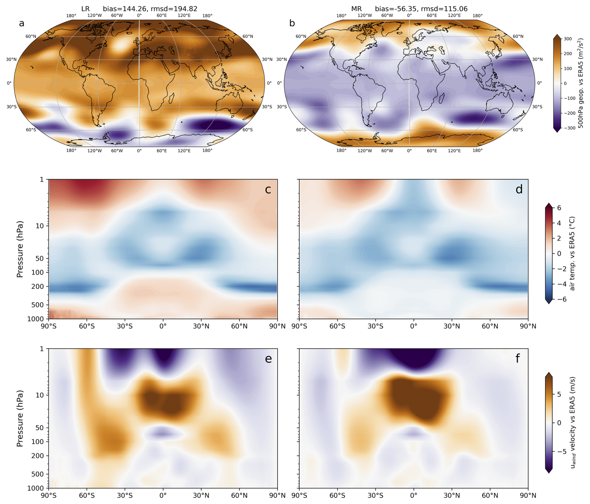
Figure 10 (a, b) 500 hPa geopotential height mean bias and global zonally averaged (c, d) air temperature and (e, f) u wind velocity biases with respect to ERA5. The biases, relative to the period 1979–2014, are shown for the low resolution (LR, left panels) and medium resolution (MR, right panels) simulations.

The global zonal-mean temperature cross-sections for the low-resolution simulation (Fig. 10c) reveal a bias structure and magnitude similar to that reported by Streffing et al. (2022). In the medium-resolution the cold biases in the upper troposphere (around 250 hPa), present in both hemispheres, persist but are reduced (Fig. 10d). An analogous, but more pronounced improvement is seen in the warm biases of the lower troposphere over polar regions as well as in the positive temperature bias in the upper stratosphere. A particularly notable change occurs in the extra-polar troposphere, where the warm bias present in the low-resolution simulation not only decreases in magnitude but also reverses sign in the medium-resolution run. The sign and vertical structure of the tropospheric temperature biases – and how they differ between the two simulations – directly explain the contrasting patterns of geopotential height bias observed in the two configurations.

In CMIP6 models, tropical tropospheric warming is typically overestimated, especially between 200 and 500 hPa. This bias has been linked to surface warm biases (Mitchell et al., 2020), as well as to excessive vertical development of convection and underestimated entrainment rates in the troposphere (Keil et al., 2021). In the medium-resolution simulation presented here, surface warming is substantially reduced, and a similar reduction is seen in the tropical troposphere. This suggests that the improved representation of convective and dynamical processes – including tropical waves, mesoscale eddies, and smaller-scale convection – helps mitigate these persistent biases.

Because of the warm bias, the low-resolution simulation underestimates the equator-to-pole temperature gradient in the troposphere (Fig. 10c), as a consequence the subtropical jet streams are displaced too far toward the poles and are simulated with excessive strength and vertical extent compared to reanalysis data (Fig. 10e). This bias is particularly pronounced in the Southern Hemisphere and helps explain the apparent decoupling between the geopotential height and tropospheric temperature biases. The overly strong, poleward-displaced, and vertically extended westerlies intensify the circumpolar trough, leading to lower geopotential heights around Antarctica despite the presence of a warm tropospheric bias.

In the medium-resolution simulation, the reduction of tropospheric temperature biases is accompanied by a substantial decrease in zonal wind biases across most latitudes and pressure levels (Fig. 10f), indicating a more realistic thermal wind balance. In contrast, biases in equatorial stratospheric winds worsen with increased resolution. The medium-resolution simulation continues to exhibit stronger-than-observed westerlies in the upper stratosphere, indicating that AWI-CM3 still struggles to adequately reproduce the easterly phase of the Quasi-Biennial Oscillation (QBO), still a challenging aspect for climate models (Richter et al., 2020; Elsbury et al., 2021). This likely affects the representation of the Semiannual Oscillation (SAO), whose variability is strongly modulated by the QBO (Jaison et al., 2024). Accordingly, the negative wind bias in the uppermost stratosphere points to an underestimated westerly phase of the SAO.

3.7 Precipitation, cloud cover and radiation fluxes

As shown by Streffing et al. (2022), most of the positive surface temperature biases can be co-located with negative biases in cloud area fraction, and consequently with an overestimation of surface shortwave radiation (Figs. 5a, i and 11b,c). This is particularly evident in the upwelling regions off the west coasts of southern Africa and South America. Interestingly, while off the coast of South America the consistent reduction in temperature bias with increasing resolution corresponds to an improved representation of clouds and, consequently, surface radiation fluxes, the situation is different off the coast of southern Africa. There, the warm bias is reduced despite a slight deterioration in the model’s representation of both clouds and radiation fluxes. A similar correspondence of patterns can be identified in the Pacific Ocean, where the temperature bias associated with the double Intertropical Convergence Zone (ITCZ) is mirrored in the bias structures of clouds, precipitation, and shortwave radiation-also as pinpointed by Streffing et al. (2022). In this low-resolution configuration of AWI-CM3, the precipitation bias is larger than the CMIP6 ensemble mean (Tian and Dong, 2020). However, increasing the model resolution leads to a considerable improvement, particularly in the tropical belt where we see an error reduction close to 20 % across all seasons (Fig. 3). A weakening of the double ITCZ bias is also visible in the medium-resolution configuration (Fig. 11a, e). Mid-to-high latitudes show a limited difference with respect to observations, in both the simulations. On a global scale a slight reduction is also observed in the shortwave radiation bias, when moving from low to medium resolution. Conversely, negative biases in clouds and longwave radiation increase in magnitude. This is primarily because the improvement in these two fields is more substantial for positive biases. Nevertheless, all the variables considered show a reduction in root mean square error (rmsd), indicating an overall improvement in model performance.

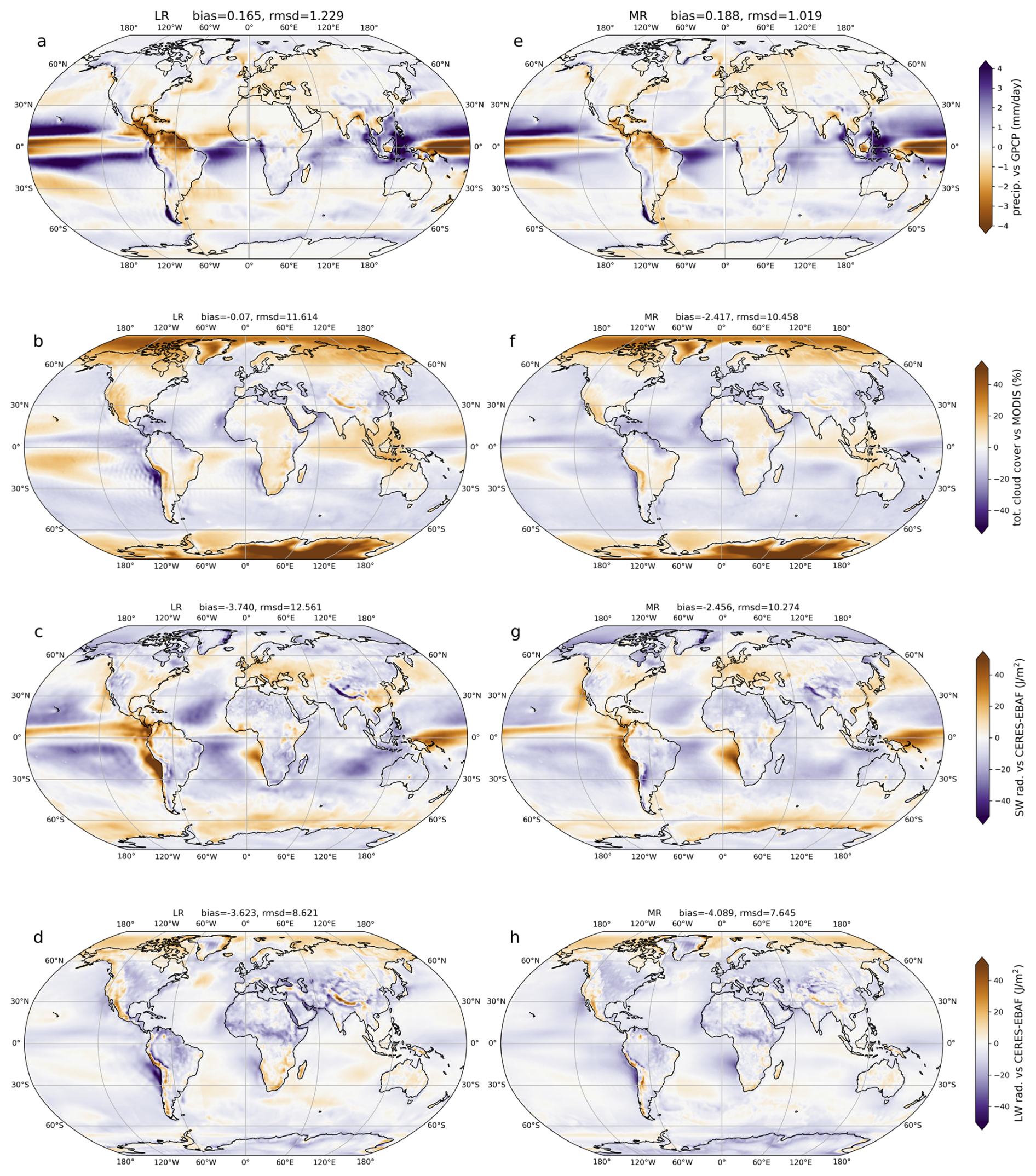
Figure 11 Annual mean (a, e) precipitation bias with respect to GPCP, (b, f) total cloud coverage bias with respect to MODIS (Platnick et al., 2015) and surface net (c, g) shortwave and (d, h) longwave radiation biases with respect to CERES (NASA/LARC/SD/ASDC, 2019; Wielicki et al., 1996). Bias and rmsd represent the area-weighted mean and root mean square difference between model and observations. Due to data availability for cloud coverage and radiation the period considered is 2000–2014, while for precipitation the period considered is 1979–2014. Results are shown for both the low resolution (LR, a–d) and medium resolution (MR, e–h) simulations.

Representing cloud cover over high latitudes remains a challenging aspect for AOGCMs. In agreement with most CMIP6 models (Lauer et al., 2023), AWI-CM3 tends to overestimate cloud cover over the Southern Ocean (Fig. 11b, f). However, this bias coexists with an overestimation of surface shortwave radiation (Fig. 11c, g), suggesting that the issue involves not only the cloud amount but also cloud properties – particularly an underrepresentation of low-level clouds or an underestimation of cloud albedo, as also noted in other CMIP6 studies (Zelinka et al., 2020; Zhao et al., 2022). Given the low surface reflectivity of the Southern Ocean, the surface albedo is particularly sensitive to cloud characteristics. Consequently, due to the strong shortwave cloud radiative cooling effect, the net cloud radiative forcing in this region is dominated by the shortwave component. This bias is likely linked to sea ice extent errors, especially during summer. For example, in the region off West Antarctica, where the positive surface shortwave radiation bias is reduced, the medium-resolution simulation shows a slight improvement in sea ice extent compared to the low-resolution configuration (Fig. A5b, d, f). Over the Arctic Basin, cloud cover overestimation has a different impact on the surface energy budget. In this region, clouds primarily act to warm the surface during winter by enhancing downward longwave radiation (Walden et al., 2017). Accordingly, AWI-CM3 shows a positive bias in surface net longwave radiation due to the excess cloud cover, while the net surface shortwave flux is underestimated (Fig. 11b–d, f–h). At lower Arctic latitudes, going from low to medium resolution, the longwave bias becomes weaker while the shortwave bias becomes more pronounced (Fig. 11c, d, g, h). This enhanced cooling effect likely contributes to the co-located overestimation of sea ice extent mentioned earlier.

Overall, it is worth noting that for all variables, the bias in the medium-resolution model configuration relative to observations is smaller in magnitude than the CMIP6 multi-model mean bias (Fig. 3). Moreover, the improvement compared to the low-resolution configuration, though modest, appears consistent across seasons and geographic regions.

3.8 The Weddell Sea atmosphere-ocean feedback

As mentioned earlier, our medium-resolution simulation shows a significant drop in September sea ice area in the Southern Ocean around year 2030, a feature not present in the low-resolution simulation (Fig. 4b). This pronounced decline, which is indicative of a strong non-linearity in the climate system, is centered in the Weddell Sea. Here approximately half of the total sea ice area is lost during the decade analyzed (Fig. 12a). In contrast, the low-resolution simulation maintains a relatively stable sea ice cover (Fig. 12i), exhibiting only slightly increased variability after mid-century and no clear decline before the last two decades of the century, consistent with the CMIP6 multi-model ensemble mean.

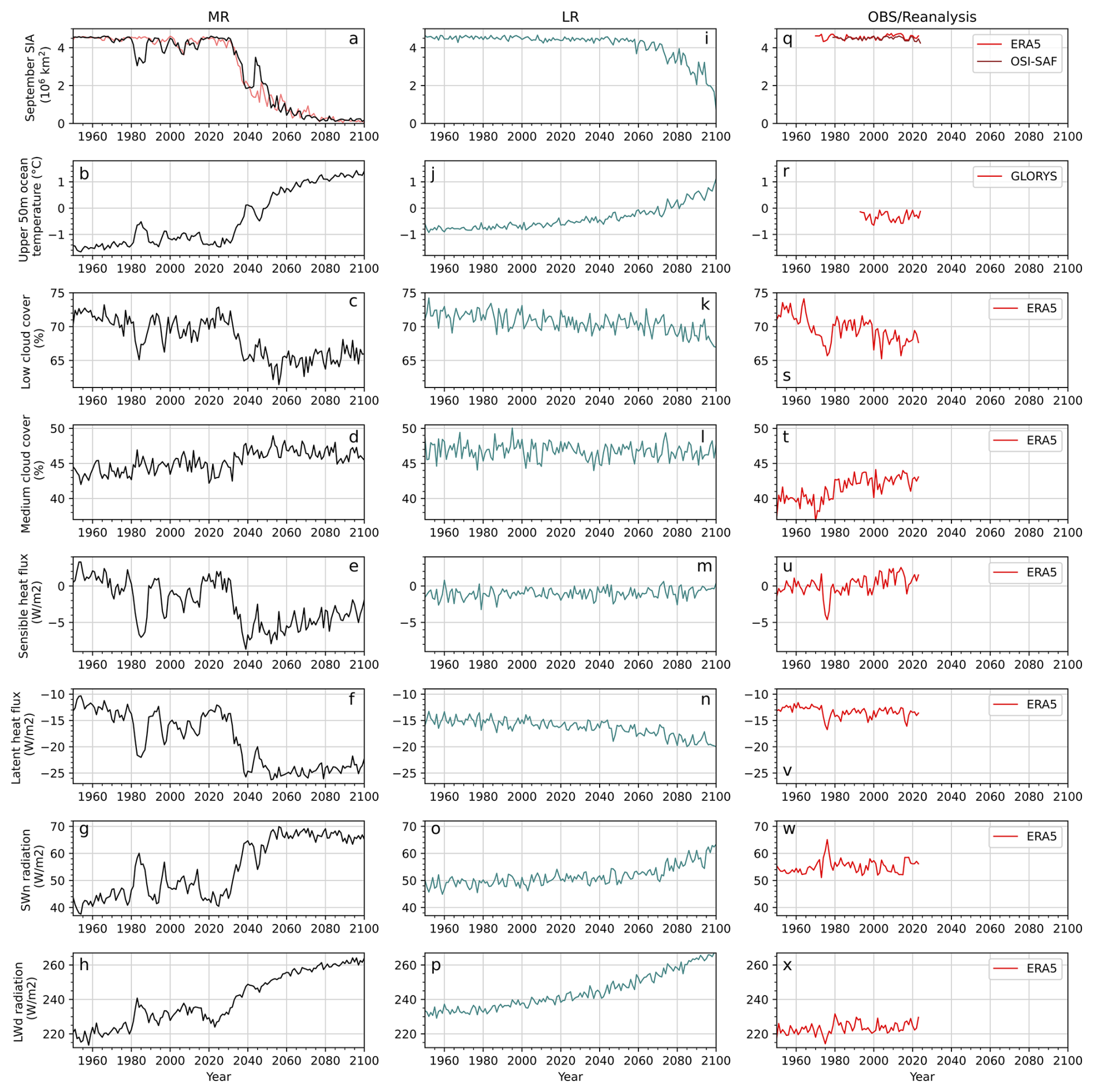
Figure 12 Time series of key variables involved in atmosphere–ocean interaction feedbacks. Panels (q)–(x) show September mean sea ice area and annual mean of upper 50 m ocean temperature, low- and mid-level cloud cover, surface sensible and latent heat fluxes, surface net shortwave radiation (SWn) and surface downward longwave radiation (LWd) over the Weddell Sea region (50° W–30° E, 60–75° S), based on observations (GLORYS, NSIDC) and reanalysis data (ERA5). Panels (a)–(p) show the same variables from the AWI-CM3 simulations at medium (TCO319-DART) and low (TCO95-CORE2) resolution. In panel (a) the light red line shows the sea ice area from the AWI-CM3 TCO319-DART simulation shown in Kim et al. (2026).

Prior to the onset of sea ice loss, upper ocean temperature increases steadily, though the trend differs between the two configurations: the low-resolution run shows a monotonic rise, while the medium-resolution simulation exhibits a step-like pattern (Fig. 12b, j). As detailed by Kim et al. (2026), this marks the onset of a cascade of ocean–atmosphere feedbacks. Increased heat release from both sea ice and the ocean – via latent and sensible heat fluxes (Fig. 12e, f) – warms the lower atmosphere. Through the lapse rate and the albedo feedbacks both tropospheric temperature and humidity shift, enhancing the surface net shortwave radiation flux (Fig. 12g) and modifying the vertical structure of the atmosphere. This affects cloud cover (Fig. 12c, d), and cloud optical depth, ultimately influencing the surface downward longwave radiation flux (Fig. 12h). Figure 12 illustrates that this chain of radiative feedbacks is well captured in our medium-resolution simulation. The AWI-CM3 model version used here closely aligns with that employed by Kim et al. (2026), and both medium-resolution simulations use the same grid resolution. This allows our simulation to be considered essentially a second realization of the one presented by Kim et al. (2026), supporting the robustness of their findings. As shown in Fig. 12a, the sea ice regime shift appears in both simulations and occurs at a similar point in time. Importantly, similar feedback signatures are also identifiable in the observational and reanalysis data analyzed (Fig. 12q–x), particularly during the well-documented polynya event of 1975/1976. These processes are evident both during smaller polynya-like events that occur before the major sea ice decline around 2030, and during the large-scale decline itself. In the latter case, the magnitude of the variability is markedly stronger, and unlike the earlier events, no recovery of sea ice extent is observed in the Weddell Sea region thereafter. In contrast, the low-resolution simulation fails to reproduce this sequence of feedbacks. Across all examined fields, it shows a persistently monotonic and stable behavior, lacking the coupled dynamical and radiative variability seen in both the medium-resolution run and observational data.

It can be noted that, when comparing the timeseries, the medium-resolution simulation tends to overestimate the amplitude of variability relative to reanalysis data. However, studies have shown that ocean reanalyses often disagree in their representation of seasonal and interannual variability (Hobbs et al., 2020; Nakayama et al., 2024), particularly on regional scales, and that Southern Ocean variability can exceed what is captured by existing reanalyses or sparse observations (Shi et al., 2021; Auger et al., 2021; Nakayama et al., 2024). In conclusion, these results support the suggestion of a potential sudden, accelerated Antarctic sea-ice decline in the coming decades, but also show the evidence for a nonlinear sea ice sensitivity to greenhouse warming, which can contribute to explain the apparent mismatch between the current generation of climate models and observations.

4 Conclusions

This study presents a comprehensive evaluation of the AWI-CM3 coupled climate model in both low-resolution (LR) and medium-resolution (MR) configurations, focusing on their ability to simulate key aspects of Earth’s climate across a range of variables, time periods, and spatial domains. Through an experimental setup in which both configurations followed the CMIP6 HighResMIP protocol and were run over the same historical and future periods, we were able to isolate and assess the impact of horizontal resolution on the model’s performance. The results reveal consistent and substantial improvements in the medium-resolution simulation, which achieved an average reduction of ∼ 28 % in climatological errors relative to the CMIP6 multi-model mean and showed superior agreement with observations across most variables, regions, and seasons.

The benefits of higher resolution are particularly evident in regions where mesoscale and submesoscale processes play a crucial role, such as the polar oceans. In the Southern Ocean, the MR configuration substantially improves the representation of sea ice dynamics, mixed-layer depth variability, and deep convection patterns, leading to more realistic simulations of polynya formation and regional heat fluxes.

The medium-resolution model also exhibits a marked regime shift in Antarctic sea ice extent in the Weddell Sea (Kim et al., 2026), triggered by ocean-atmosphere feedbacks, which is absent in the LR simulation and most CMIP6 models. This underscores how higher-resolution models, with eddy-resolving oceans and improved atmospheric representation, can capture emergent behaviors and abrupt climate transitions that may be overlooked in lower-resolution configurations (Roberts et al., 2025). Such capability is of increasing concern in light of the rapid and potentially irreversible environmental changes observed in recent years in Antarctica (Abram et al., 2025). This is particularly important also given that it remains uncertain whether upcoming AI-based climate models will be able to accurately reproduce feedback processes or identify potential sudden regime shifts.

In the Northern Hemisphere, the MR simulation offers improved spatial and temporal representations of sea ice variability, although some biases – such as the overestimated September sea ice extent in mid-latitudes – persist. Across the tropics and mid-latitudes, increased resolution leads to a more accurate depiction of surface temperature trends, precipitation patterns, and ocean heat content, although improvements are regionally dependent and sometimes accompanied by enhanced variability. In terms of atmospheric dynamics, the MR model reduces longstanding biases in tropospheric temperature and zonal wind fields, leading to a more realistic thermal wind balance and an improved simulation of the subtropical jet streams. While stratospheric biases, particularly related to the Quasi-Biennial Oscillation (QBO), remain, overall fidelity in large-scale circulation features is markedly enhanced.

One of the more compelling findings of this study is the improvement in ocean circulation patterns and volume transports through major straits and channels in the MR simulation. Enhanced resolution enables the model to better resolve mesoscale eddies and vertical mixing processes, leading to more realistic simulations of features such as the Atlantic Meridional Overturning Circulation (AMOC), Arctic outflows, and Antarctic Bottom Water (AABW) formation. These enhancements contribute to a more accurate portrayal of heat and salt transport across ocean basins, as well as feedbacks between sea ice, ocean dynamics, and the atmosphere.

Medium-resolution simulations offer several advantages, including a more detailed representation of interannual to decadal variability and feedback processes, which can reveal different potential trajectories for the climate system and provide a richer picture of possible climate outcomes. This enhanced variability, at the same time, can make it more challenging to attribute forced trends and separate signal from internal noise. As noted earlier, only a single ensemble member was run and analyzed. The higher computational cost makes it more challenging – albeit not impossible – to generate large ensembles, which are important for robust uncertainty quantification and for assessing the statistical significance of model responses. Consequently, relying on a single simulation realization inherently constrains the ability to fully sample internal climate variability or to disentangle stochastic fluctuations from externally forced changes. Nonetheless, even a single MR simulation allows us to formulate hypotheses and gain valuable insights into model performance, emergent behavior, and potential climate responses. It highlights the strengths of higher resolution while identifying areas where ensemble approaches could further strengthen confidence in projections.

In conclusion, our findings emphasize the importance of increased horizontal resolution in improving the fidelity of coupled climate simulations, particularly in regions where small-scale processes and feedback mechanisms are critical. The MR configuration of AWI-CM3 demonstrates a clear step forward in reproducing observed climatology, resolving nonlinear climate dynamics, and capturing potential tipping points in the Earth system. As the climate modeling community advances toward CMIP7 and future generations of Earth system models, our results advocate for the integration of at least medium-resolution (or higher) modeling as a complementary strategy to traditional multi-model ensembles. These efforts, paired with rigorous observational benchmarking and continued refinement of parameterizations, will be essential in reducing uncertainties in climate projections and improving the credibility of climate change assessments.

Appendix A: Additional Figures

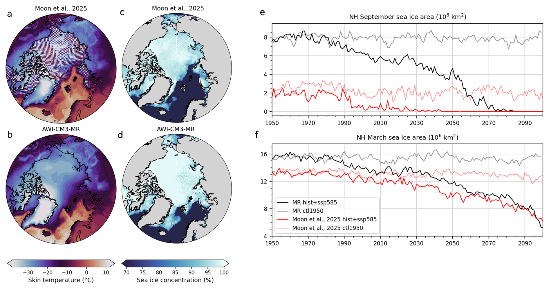
Figure A1 Comparison of skin temperature and sea ice concentration for the area north of 60° S, as well as total September/March sea ice area, between the TCo319L137-DART simulation described in Moon et al. (2025) and the AWI-CM3-MR simulation evaluated in this study. The aim is to highlight improvements resulting from the modified interpolation method for sea ice heat fluxes. Skin temperature is shown as the monthly mean for March 2000, while sea ice concentration is shown as the daily mean for 1 March 2000.

Table A1 List of CMIP variables used in Figs. 3 and A2 given together with their corresponding standard names and units.

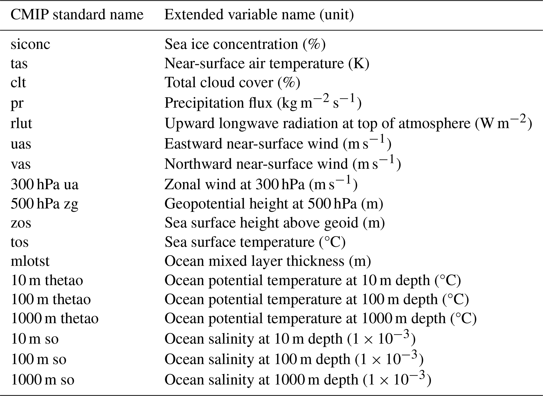
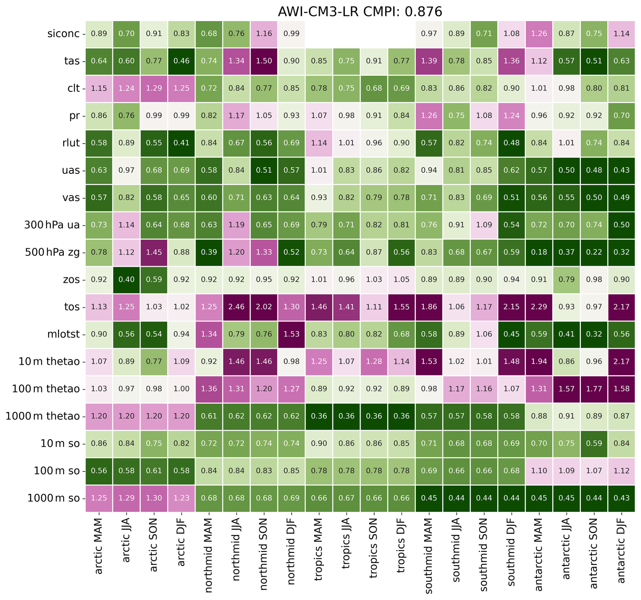
Figure A2 Performance indices that give the absolute error in 1989–2014 AWI-CM3 historic climatology as a fraction of the absolute error averaged over CMIP6 models (Streffing et al., 2025; Reichler and Kim, 2008). Values below (above) 1 correspond to below (above) CMIP6 average biases. The indices here reported are computed for the low (AWI-CM3-LR) resolution simulation. The Arctic and Antarctic regions are the areas north of 60° N and south of 60° S, respectively. The mid-latitudes span between 30 and 60° in both hemispheres, while the tropical region lies between 30° N and 30° S.

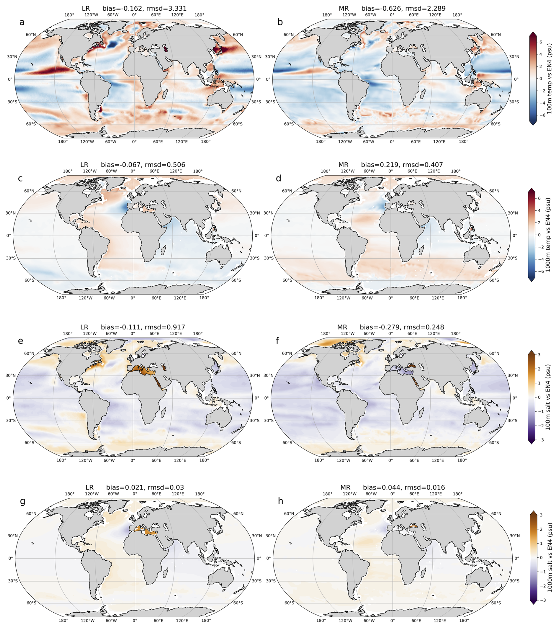
Figure A3 Ocean (a–d) temperature and (e–h) salinity biases with respect to EN4 dataset at 100 and 1000 m depth. The biases, relative to the period 1979–2014, are shown for the low resolution (LR, left panels) and medium resolution (MR, right panels) simulations.

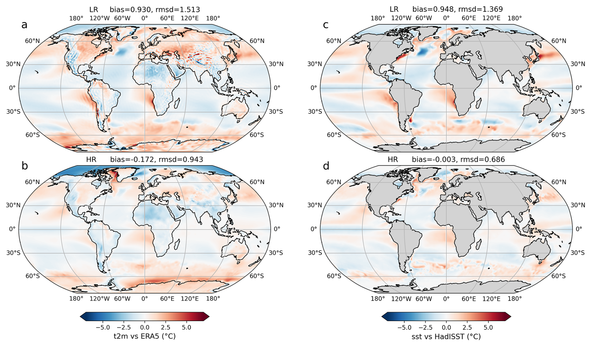
Figure A4 Annual mean 2 m air temperature (a, b) and sea surface temperature (c, d) biases (global mean bias removed) for the period 1979–2014 relative to ERA5 and HadISST, respectively. Results are shown for both the low-resolution (LR) and medium-resolution (MR) experiments.

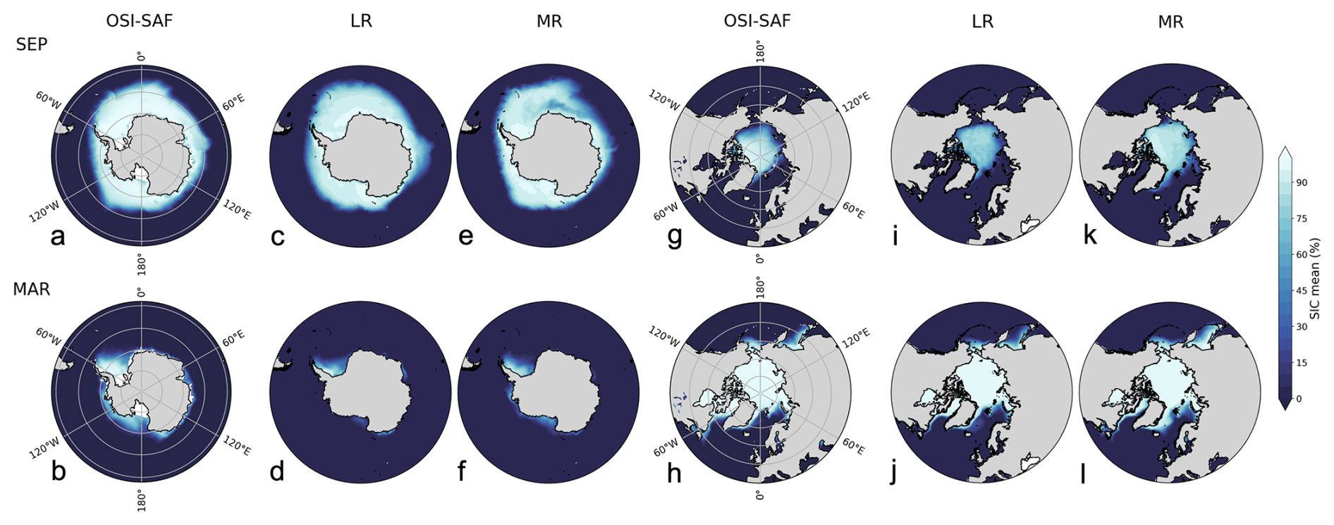
Figure A5 Means of March and September sea ice concentration from 1979 to 2014 are shown for both hemispheres, based on OSI-SAF observations (a, b, g, h) and simulations from the low-resolution (LR, c, d, i, j) and medium-resolution (MR, e, f, k, l) model configurations.