A Geographically Weighted Gaussian Process Regression (GW-GPR) emulator of anthropogenic PM_2.5 from the GEOS-Chem High Performance (GCHP) 13.0.0 global chemical transport model

Chemical transport modelling has been an essential tool to study the impacts of socio-economic changes and policies on air quality and associated social costs due to human health impacts. However, high computational and human resource demands limit the use of state-of-the-art chemical transport models outside of the atmospheric science community. We address this limitation by training Geographically Weighted Gaussian Process Regressors (GW-GPR) on the outputs of a series of perturbation experiments from the GEOS-Chem High Performance global chemical transport model (GCHP 13.0.0). The Gaussian Process Regressor relates changes in annual mean surface anthropogenic PM_2.5 in each GCHP model grid cell to changes in short-lived air pollutant emissions and atmospheric CH₄ and CO₂ concentrations. In comparison to existing linearized and regionalized approaches, our method can account for sub-regional changes in air pollutant emission patterns and incorporates the non-linear response of secondary air pollutants to precursor and greenhouse gas emissions. We evaluate our emulator by predicting the global distribution of PM_2.5 in 2050 (relative to 2014) under 4 sets of climate and air pollution control policy scenarios. The emulator reproduces grid cell scale changes in anthropogenic PM_2.5 (R²=0.94–0.99 over the 4 scenarios tested), and associated global changes in premature mortalities at 95 % confidence level, while requiring <10 s of CPU time (vs. ∼3000 CPU hours for GCHP) for each scenario. We demonstrate the utility of the emulator by projecting global trends of population-weighted PM_2.5 from the AerChemMIP ensemble, where the emulator prediction falls within the ensemble range. To our knowledge, the GW-GPR emulator is the first global-scale emulator operating at grid cell scale with explicit consideration of non-linearities in atmospheric chemistry, climate change, and provides predictive uncertainties. The accuracy, speed and simplicity of the emulator also show the capability of machine learning algorithms in emulating global atmospheric chemistry models, and in making atmospheric chemistry modelling accessible for global climate/air pollution scenario analysis and integrated assessment.

1 Introduction

Fine (aerodynamic diameter ≤ 2.5 µm) particulate matter (PM_2.5) is among the most important air pollutants at global scale, threatening both human and ecosystem health. Globally, PM_2.5 exposure was estimated to be responsible for ∼4 million deaths in 2019 (Sang et al., 2022), and addressing health and environmental impacts from ambient air pollution has been included within the Sustainable Development Goals (goal 3.9.1 and 11.6.2) (United Nations, 2015). The conventional approach to evaluate the impacts of socio-economic changes and policy interventions on air quality involves producing the projected air pollutant emission inventories (and meteorological fields if direct impacts of climate change are considered) and feeding them as inputs to a chemical transport model to simulate the impacts on air pollutant concentration. Alternatively, the greenhouse gas (GHG) emission or concentration, and air pollutant emissions can be directly fed into chemistry-climate models or Earth system models to further include the feedback between atmospheric composition and other components of Earth system. This process is highly demanding in terms of human and computational resources, which limits its usage for policy analysis and integrated assessment.

To increase the accessibility of air quality modelling for the broader scientific and stakeholder communities, strategies have been developed to reduce the complexity of air quality modelling by drawing from full chemical transport model experiments, resulting in various reduced-form air quality models that are faster and easier to run while retaining reasonable accuracy. One approach involves dividing the world into regions. By assuming a linear relationship between air pollutant emissions in one region (source) and the air pollutant concentrations in other regions (receptor), source-receptor (SR) matrices are constructed by running a series of chemical transport model experiments with emission perturbed individually at each region. The SR matrices can then be used as a linearized global air quality model. This approach is also useful in spatial attribution of air pollution, which is applied in the Task Force on Hemispheric Transport of Air Pollutants (HTAP) (Galmarini et al., 2017; Liang et al., 2018). Designed to be a useful tool for science-policy analysis, the TM5-FASST model (Van Dingenen et al., 2018) computes SR matrices for 56 regions of the world, and subsequently processes the output into public health, agriculture and climate impact metrics. Another approach involves using output of full complexity chemical transport model to parameterize some physical and chemical processes, resulting in a reduced-order chemical transport model that can be run faster and with higher resolution, which are applicable for regional and global high-resolution (∼1–4 km) modelling with runtime of a few hundred CPU hours per model year (Tessum et al., 2017; Thakrar et al., 2022),. These SR and reduced-order models have been frequently applied in recent science and policy studies (e.g. Camilleri et al., 2023; Huang et al., 2023; Reis et al., 2022), showing the utility and demand for these outputs.

However, both SR and reduced-order models rely on several simplifying assumptions, which do not always hold. Many methods rely on linearizing the relationship between emissions and concentrations, which has been shown to be a reasonable approximation when the emission change is relatively small (Van Dingenen et al., 2018), but the formation rate of major secondary air pollutants such as inorganic PM_2.5 (Ansari and Pandis, 1998) are known to respond non-linearly to precursor emissions, especially when there are shifts in sulphate-nitrate-ammonium chemical regimes. This issue can be relevant when exploring a wide range of climate and air quality scenarios given the large range of possible air pollutant emissions and the discrepancy in the rates of change of different precursor emissions (NO_x vs. NH₃ vs. SO₂ for inorganic PM_2.5) (Atkinson et al., 2022a; Rao et al., 2017; Turnock et al., 2020). Existing SR matrices and reduced-order models also often ignore the effects of climate change on air pollution (e.g. changing precipitation and associated wet deposition, temperature effects on gas-aerosol partitioning and oxidation chemistry) (Jacob and Winner, 2009). Garcia-Menendez et al. (2015) find that under a high-warming scenario, climate change alone can increase population-weighted annual average PM_2.5 by 1.5 µg m⁻³ between 2000 and 2100 over the contiguous United States.

Recent innovations in regional reduced-form air quality models have moved beyond simple linear scaling, by applying non-linear regression techniques. Conibear et al. (2022) and Vander Hoorn et al. (2022) successfully used Gaussian Process Regression to emulate the grid cell scale response of annual mean PM_2.5 to a large range (−100 % to +50 %) of sectoral emission perturbations over China and the Perth greater metropolitan region respectively, with regional chemical transport model perturbation experiments as training data. Colette et al. (2022) applied multivariate quadratic regressions to emulate the simulated PM_2.5 response to emission control policies over Europe, achieving an accuracy of <2 % relative error in 95 % of grid cells. Meanwhile, a geographically weighted (i.e. using a weighted sum of regional emission changes as predictors to represent pollutant transport process) linear regression emulator was shown to reproduce PM_2.5 response to precursor emissions from the parent chemical transport model within 10 % accuracy over Europe (Pisoni et al., 2017).

Building on these regional scale applications, we combine Geographic Weighting and Gaussian Process Regression (GW-GPR) techniques to emulate the output of a global chemical transport model, GEOS-Chem High Performance (GCHP) driven by meteorological data from multiple climate simulations with the Community Atmosphere Model (CAM, collectively GCHP-CAM) (Eastham et al., 2023). This results in a global reduced-form anthropogenic PM_2.5 model that can account for spatially heterogenous pollutant emission changes and non-linearity in atmospheric chemistry under multiple climate scenarios without requiring simulated meteorological fields as input, and provide robust uncertainty estimates, without drastically increasing the computational cost. These properties would make our reduced-form model a highly viable candidate for specific use cases (e.g. ensemble modelling, building interactive tools, embedding in integrated assessment workflows).

2 Method

We emulate the response of annual mean surface anthropogenic PM_2.5 to changes in air pollutant emissions and climate modelled by a global chemical transport model, GEOS-Chem High Performance (GCHP). Here, we provide descriptions for our GCHP model setup and experiments, and the process of constructing and evaluating the emulator.

2.1 MIT Integrated Global System Model (IGSM) and its coupling with Community Atmosphere Model (CAM)

The climate scenarios are generated from the MIT IGSM framework (Fig. 1). The human system component of IGSM, the Economic Projection and Policy Analysis model version 7 (EPPA7) (Chen et al., 2022), is a global multi-sector (22 sectors) multi-region (18 regions) recursive-dynamic computable general equilibrium model. EPPA provides regionalized and sectorized consumption of different fuel types under the socioeconomic assumptions of each scenario. The associated greenhouse gas (GHG) and air pollutant emissions drive the MIT Earth System Model (MESM) (Sokolov et al., 2018) to simulate yearly global average atmospheric GHG concentration, and concentrations of zonally averaged climate and near-term climate forcers (NTCF, e.g. aerosols, O₃).

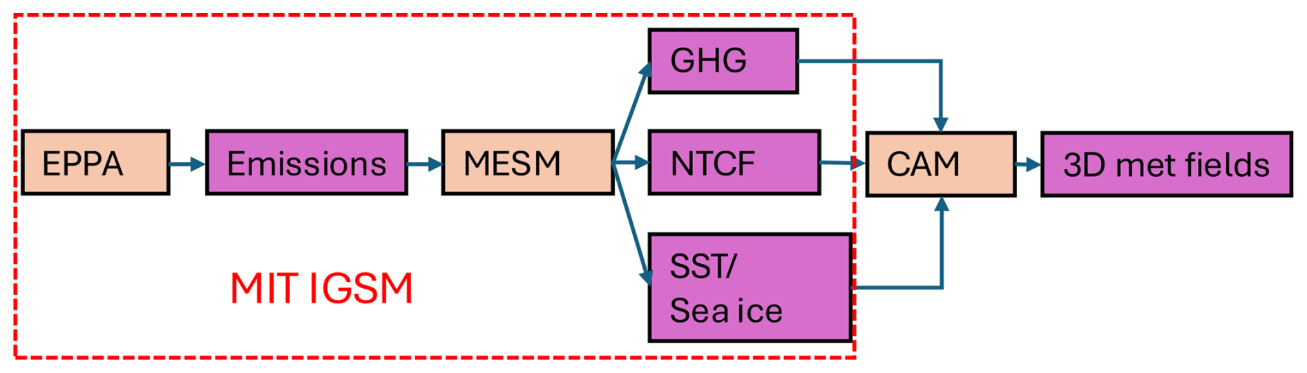
Figure 1 Schematic of the IGSM-CAM modelling framework. Orange boxes represent modelling systems, purple boxes represent data sets. The red dashed box represents the MIT IGSM part of the framework.

Since the output of IGSM is zonally-averaged, we simulate 3D meteorological fields using the IGSM-CAM framework (Monier et al., 2013) that links the IGSM to the National Center for Atmospheric Research Community Atmosphere Model (CAM) 3.1 (Collins et al., 2006). In this framework, CAM is driven by the IGSM output GHG concentrations, sea surface temperature anomalies, sea ice cover, and NTCF concentrations (Fig. 1). A pattern scaling algorithm is used to translate 2D NTCF output from IGSM to the 3D input fields required by CAM. The simulation outputs used in this study are described and evaluated in detail by Monier et al. (2015). IGSM-CAM is run with a horizontal resolution of 2°×2.5° on 26 vertical layers up to 2.2 hPa.

2.2 GEOS-Chem High Performance model driven by CAM meteorological fields (GCHP-CAM)

We use the GCHP-CAM modelling system, which was described and evaluated in Eastham et al. (2023), to simulate global PM_2.5 distribution, and its response to climate and pollutant emission changes. The modelling system is based on a customized version of GCHP 13.0.0 (The International GEOS-Chem User Community, 2021) that can be driven by the modelled meteorological fields derived from the IGSM-CAM framework. Here we provide a brief description of the modelling system and specific setups for our work.

GCHP (Eastham et al., 2018) simulates PM_2.5 by resolving the chemistry, transport, emission and deposition of relevant chemical species. Oxidant chemistry is simulated using a coupled VOC–CO–NO_x–O₃–aerosol-halogen chemical mechanism (Sherwen et al., 2016). GCHP is run at C48 (∼200 km) horizontal resolution with the same vertical layers with the IGSM-CAM simulations. The model output is remapped into a 2° latitude × 2.5° longitude horizontal grid conservatively (Jones, 1999). PM_2.5 includes contribution from nitrate, sulphate, ammonium, black carbon (BC), organic carbon (OC), fine dust, sea salt and secondary organic aerosols (SOA). The formation of secondary inorganic aerosols is simulated by considering the thermodynamic equilibrium of the NH${}_{\mathrm{4}}^{+}$–Na⁺–SO${}_{\mathrm{4}}^{\mathrm{2}-}$–NO${}_{\mathrm{3}}^{-}$–Cl⁻–H₂O system through ISORROPIA II (Fountoukis and Nenes, 2007). Organic aerosols are assumed to be non-volatile. SOA formation follows a simple yield-based scheme that converts a fixed potion of isoprene, monoterpenes and other terpenoids into a lumped SOA precursor pool and another lumped SOA pool (Kim et al., 2015).

Biogenic volatile organic compounds (BVOC) emissions follow Guenther et al. (2012) with isoprene inhibition by CO₂ .(Possell and Hewitt, 2011; Tai et al., 2013) included. Soil NO_x emissions follow Hudman et al. (2012). While BVOC and soil NO_x emissions are both calculated online (and therefore respond to climate and atmospheric CO₂ concentration), mineral dust (Meng et al., 2021), lightning NO_x (Murray et al., 2012) and wildfire (from Global Fire Emission Database, version 4.1; Van Der Werf et al., 2017) emissions are held at 2014 level.

Aerosol concentrations are archived at daily time resolution, and subsequently processed into annual mean surface total anthropogenic PM_2.5. Total PM_2.5 mass (Eq. 1) is calculated from the aerosol concentration by considering aerosol hygroscopic growth at 35 % relative humidity, aligning with the PM_2.5 measurement standard of the United States Environmental Protection Agency (USEPA) (Latimer and Martin, 2019). Anthropogenic PM_2.5 mass (Eq. 2) is calculated by the above method, but only summing a subset of aerosol species (sulphate, nitrate, ammonium, BC and OC) while omitting other aerosol species that are driven by non-industrial sources (dust, sea salt and SOA):

$$\begin{array}{}\text{(1)}& {\displaystyle }\begin{array}{rl}\mathrm{Total}{\mathrm{PM}}_{\mathrm{2.5}}& =\mathrm{1.1}\left({\mathrm{NH}}_{\mathrm{4}}^{+}+{\mathrm{NO}}_{\mathrm{3}}^{-}+{\mathrm{SO}}_{\mathrm{4}}^{\mathrm{2}-}\right)+\mathrm{BC}+\mathrm{OC}\\ & +\mathrm{fine}\mathrm{mineral}\mathrm{dust}+\mathrm{SOA}+\mathrm{1.86}\left(\mathrm{Sea}\mathrm{Salt}\right)\end{array}\text{(2)}& {\displaystyle }\begin{array}{rl}\mathrm{Anthropogenic}{\mathrm{PM}}_{\mathrm{2.5}}& =\mathrm{1.1}\left({\mathrm{NH}}_{\mathrm{4}}^{+}+{\mathrm{NO}}_{\mathrm{3}}^{-}+{\mathrm{SO}}_{\mathrm{4}}^{\mathrm{2}-}\right)\\ & +\mathrm{BC}+\mathrm{OC}.\end{array}\end{array}$$

2.3 Generating PM_2.5 training data using GCHP-CAM

We conduct GCHP-CAM simulations for atmospheric composition for the year 2014 (with additional 3 months of simulations as spin up (output discarded) before the start of 2014) by applying IGSM-CAM simulated meteorology, anthropogenic emissions of air pollutants from the Community Emission Data System (Hoesly et al., 2018), and the monthly surface CH₄ concentration derived by spatially kriging the observations from National Oceanic and Atmospheric Administration Global Monitoring Laboratory Cooperative Air Sampling Network for 2014. The resulting modelled total and anthropogenic PM_2.5 concentrations serve as a baseline for subsequent comparisons.

To effectively sample the sensitivity of PM_2.5 over a wide range of climate and air pollution emissions, we generate the training set from a series of GCHP-CAM perturbation experiments by manipulating 9 input variables that affect PM_2.5 and oxidant concentration: 7 air pollutant emissions – NO_x, SO₂, NH₃, NMVOC, BC, OC, carbon monoxide (CO) – that are commonly provided by integrated assessment models (Gidden et al., 2019), CH₄ concentration, and global warming.

2.3.1 Parameterizing global warming

Representing the direct impacts of climate change is an important aspect of building climate-aware reduced-form atmospheric composition models. However, unlike the other 8 perturbed variables, global warming cannot be directly implemented as a scaling factor in GCHP-CAM. Some recent studies achieve this goal by including 3D meteorological fields from climate model output as predictors (e.g. Li et al., 2022, 2026). However, this could limit the utility of the model to scenarios where climate model outputs are archived in a correct format. We use a simpler parameterization of climate effects in our emulator to expand its applicability.

We use the GHG concentration and IGSM-CAM simulated meteorological fields from its high-warming “REF” scenario (10 W m⁻² in 2100, resulting in 4.3 °C warming in 2080–2100 vs. 1990–2009) to provide samples across a wide range of global warming and GHG concentration from 2000–2100. While climate change can affect PM_2.5 through pathways other than simply warming (e.g. precipitation, regional stagnation, mixing depth) (Jacob and Winner, 2009), changes in meteorological variables due to well-mixed GHG forcing can usually be parameterized as spatially-varying functions (“patterns”, which are specific to individual climate models) of global mean temperature (e.g. Lütjens et al., 2025), which is a function of total radiative forcing by GHG (with climate sensitivity specific to each climate/Earth system model).

Therefore, the effects of GHG-forced climate change on PM_2.5 can be parameterized by total radiative forcing by GHG (TRF), which largely simplifies the statistical modeling and increases its applicability by not requiring meteorological variables as inputs. This implies the relation between GHG-forced climate change and PM_2.5 can be statistically learned by regression algorithms at each grid cell, when TRF is included as one of the input variables.

In our emulator, we further parameterize TRF as atmospheric CO₂ concentration. In many climate scenarios, CO₂ is projected to dominate (68 %–85 %) TRF and its trend in the 21st century (Meinshausen et al., 2020). In addition, atmospheric CO₂ concentration also directly affects isoprene emission, which could affect atmospheric oxidant (e.g. OH, O₃) (e.g. Tai et al., 2013), and therefore potentially secondary inorganic aerosol formation.

Parameterizing climate effects as TRF/CO₂ concentration allows our statistical model to include climate effects without explicitly requiring meteorological fields as input, which makes our emulator easy to integrate within the workflow of integrated assessments and ensemble modelling/emulation. However, this introduces some potential sources of systematic errors: (1) atmospheric CO₂ concentration can misrepresent TRF under climate scenarios where the trend of CO₂ emission is decoupled with the trends of other GHG emissions; (2) the assumption of time-invariant local relationship between global mean temperature/TRF and local climate variables breaks down under overshoot scenarios and over locations with strong changes in local forcing (e.g. aerosol) and energy balance (e.g. albedo feedback, land use and land cover change) (Giani et al., 2024). While the influence of pollutant emissions on PM_2.5 under these scenarios can still be properly represented by our statistical model, the result from our emulator should be interpreted more cautiously under these types of climate scenarios. More advanced methods to parameterize climate effects (e.g. using cumulative GHG emissions, combining information from climate emulators) could be further explored in future work.

2.3.2 Generating training dataset through GCHP-CAM perturbation experiments

We generate 120 sets of scaling factors for the 9 input variables (range displaced in Table 1) following a Latin Hypercube Sampling (LHS) (McKay et al., 1979) strategy. However, the changes in emissions of different pollutants are correlated, since different air pollutants often share similar emission sources (e.g. combustion). To account for co-emissions of air pollutants, we calculate the spatial correlations of the emissions of the 7 air pollutants from CEDS between 2000 and 2017. The correlation of CH₄ and global warming with other variables are set to be 0 to provide independence between climate and air pollution control policies. We then use the Iman–Conover Transform (Conover and Iman, 1982) to impose the correlation matrix for the independent and uncorrelated pairs of LHS scaling factors. The Iman–Conover Transform first transforms the sample pairs to an approximately multivariate normal distribution. Then Cholesky decompositions are used to impose the correlation matrix on the distribution, resulting in a matrix that can be applied to rearrange the sample pairs by ranking. This results in correlated pairs of scaling factors (Fig. 2) that allow us to focus on sampling the more probable parts of the input space (due to co-emissions), while preserving the marginal distributions of individual variables (i.e. uniform distribution over their respective ranges).

Table 1 Range of scaling factors and CO₂ concentration of the perturbation experiments. The range of atmospheric CO₂ concentration is derived from the range of CO₂ concentration between 2000–2100 under the “REF” scenario.

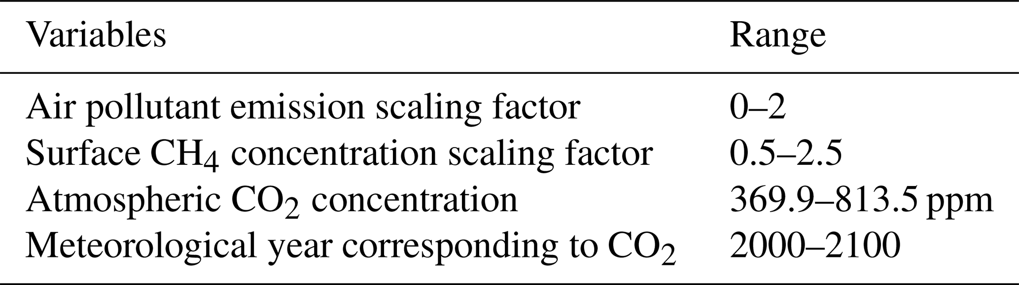
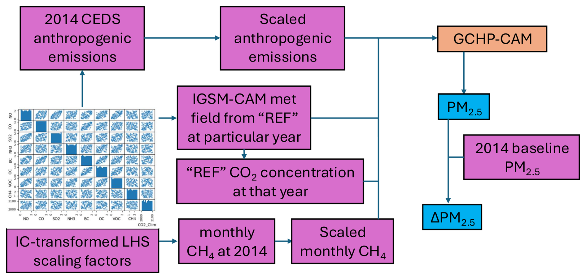
Figure 2 Schematic of generating the training set by GCHP-CAM perturbation experiments using an Iman–Conover (IC) transformed Latin Hypercube Sampled (LHS) scaling factors. The orange box represents existing modelling systems, purple boxes represent data sets, and blue boxes represents output of the perturbation experiments.

Figure 2 summarizes the workflow of the perturbation experiments. A 1-year perturbation simulation, again with an extra 3 months before as spin-up, is performed for each pair of global scaling factors applied to 2014 anthropogenic air pollutant emissions and surface CH₄ concentration. The CO₂ concentration is directly applied to calculate isoprene inhibition, and the corresponding climate effects are represented through driving the simulation with the IGSM-CAM simulated meteorological data from the year with the closest CO₂ concentration under “REF” scenario (e.g. a perturbation experiment having a CO₂ concentration of 446 ppm is driven by the IGSM-CAM simulated meteorological data at 2030 under “REF” scenario, as 2030 has the closet CO₂ concentration to 446 ppm among all years under “REF” scenario). The GCHP-CAM output we aim to emulate – changes in annual mean anthropogenic PM_2.5 concentration relative to 2014 baseline (ΔPM_2.5) – is calculated for each perturbation experiment as the training data set.

2.4 Training the Geographically Weighted Gaussian Process Regression (GW-GPR) emulator

We use Gaussian Process Regression (GPR) (Williams and Rasmussen, 1995) to relate the changes in pollutant emissions and climate with the corresponding changes in annual mean PM_2.5 concentration at grid cell scale, because of its effectiveness in handling non-linearity, good performance with small training set, and quantifying predictive uncertainties. GPR is a non-linear and non-parametric regression algorithm that does not require prior assumptions of the functional relationship between input and output variables. Instead, predictions are made by assuming the training and prediction sets follow a joint multivariate normal distribution (N):

$$\begin{array}{}\text{(3)}& \left(\begin{array}{c}{\mathit{Y}}_{\mathrm{1}}\\ {\mathit{Y}}_{\mathrm{2}}\end{array}\right)=N\left(\begin{array}{c}{\mathit{\mu }}_{\mathrm{1}},{\mathbf{\Sigma }}_{\mathrm{11}},{\mathbf{\Sigma }}_{\mathrm{12}}\\ {\mathit{\mu }}_{\mathrm{2}},{\mathbf{\Sigma }}_{\mathrm{21}},{\mathbf{\Sigma }}_{\mathrm{22}}\end{array}\right)\end{array}$$

where Y₁ is the random variable representing the prediction, and Y₂ is the random variable representing the response from training set. μ₁ and μ₂ are their means, and Σ₁₁, Σ₁₂, Σ₂₁, Σ₂₂ are the covariance matrix blocks. The prediction process can be viewed as finding (${\mathit{Y}}_{\mathrm{1}}|{\mathit{Y}}_{\mathrm{2}}=a)\sim N({\mathit{\mu }}^{\prime },{\mathbf{\Sigma }}^{\prime })$, where a is the model output from training set. Thus, the mean (μ^′) and variance (Σ^′) of the prediction can be calculated as:

$$\begin{array}{}\text{(4)}& {\displaystyle }& {\displaystyle }{\mathit{\mu }}^{\prime }={\mathit{\mu }}_{\mathrm{1}}+{\mathbf{\Sigma }}_{\mathrm{12}}{\mathbf{\Sigma }}_{\mathrm{22}}^{-\mathrm{1}}\left(\mathit{a}-{\mathit{\mu }}_{\mathrm{2}}\right)\text{(5)}& {\displaystyle }& {\displaystyle }{\mathbf{\Sigma }}^{\prime }={\mathbf{\Sigma }}_{\mathrm{11}}-{\mathbf{\Sigma }}_{\mathrm{12}}{\mathbf{\Sigma }}_{\mathrm{22}}^{-\mathrm{1}}{\mathbf{\Sigma }}_{\mathrm{21}}.\end{array}$$

By setting the prior mean of prediction as 0 and proper normalization during training process, μ₁ and μ₂=0. Then μ^′ is essentially a sum of a weighted by the correlations between the training and prediction vectors (${\mathbf{\Sigma }}_{\mathrm{12}}{\mathbf{\Sigma }}_{\mathrm{22}}^{-\mathrm{1}}$). The elements of the correlation matrix take the form:

$$\begin{array}{}\text{(6)}& {\mathit{\sigma }}_{ij}=k\left({\mathit{\theta }}_i{\mathit{\theta }}_j\right)\end{array}$$

where θ_i and θ_j are the input vectors at each training (i) or prediction (j) point, and k is the covariance function that can be chosen to control the shape and smoothness of the prediction. We use a sum of anisotropic (in the input space, not the physical distance described below) functions to represent the nature of our problem. These are smooth functions (rational quadratic function) with unknown points of chemical regime change + local interactions among variables (Matern 3/2 function) + noise from climate variability (white noise). “Training” the GPR essentially means optimizing the parameters of the covariance function k against the training data set.

We use the GPR as implemented in Scikit-learn version 1.3.2 (Pedregosa et al., 2011), and only train a GPR model for each populated (population density >1 person per km²) model grid cell. As the predictions are random variables, the uncertainty and confidence interval of each prediction can be calculated its standard deviation.

To emulate the process of chemical transport of emitted species, an isotropic 2D geographic weighting scheme is applied to calculate the effective air pollutant emission changes ($\mathrm{\Delta }{E}_{\mathrm{weighted},x,i}$) at each grid cell x for each pollutant i:

$$\begin{array}{}\text{(7)}& \mathrm{\Delta }{E}_{\mathrm{weighted},x,i}=\sum _{y_k}{e}^{-d_{y,x}^{\mathrm{2}}/\mathrm{2}{L}_i^{\mathrm{2}}}\mathrm{\Delta }{E}_{y,i}\end{array}$$

where ΔE_y,i is the emission change of pollutant i at individual grid cells considered within the dispersion range y_k (set to be within of 10 L_i of x for computational efficiency), d_y,x is the distance between grid cell y and x, and L_i is the dispersion length scale for pollutant i. Formally speaking, this implies at each grid cell x, our GW-GPR framework (f_x) predicts GCHP-CAM simulated ΔPM_2.5 using ΔE_weighted,x (the vector of $\mathrm{\Delta }{E}_{\mathrm{weighted},x,i}$ for all pollutants), and atmospheric CH₄ and CO₂ concentration as input:

$$\begin{array}{}\text{(8)}& \mathbf{\Delta }{\mathrm{PM}}_{\mathrm{2.5}}\left(x\right)=f_x\left(\mathrm{\Delta }{E}_{\mathrm{weighted},x},{\mathrm{CH}}_{\mathrm{4}},{\mathrm{CO}}_{\mathrm{2}}\right).\end{array}$$

The geographic weighting scheme is implemented by the Gaussian Blurring algorithm as in Scipy version 1.10.1 (Virtanen et al., 2020). The input variables are normalized by their corresponding global maximum value after the geographic weighting. Since the output variables are not geographically weighted, and μ₂=0 simplifies computation, the output variables are normalized by local mean and maximum at each grid cell. We note that some previous regional studies (e.g. Pisoni et al., 2017) have treated the parameters of the geographic weighting scheme as optimizable hyperparameters. However, our GCHP-CAM experiments are conducted with uniform global scaling factors for emission fields. After the variable normalization procedure, training configurations with different geographic weighting scheme would effectively collapse to the same 120 sets of global scaling factors prescribed in the GCHP-CAM experiments. Therefore, our training set cannot be used to directly optimize L_i.

Instead, we choose a globally uniform set of L_i as an approximation: $L_{{\mathrm{NO}}_x}$, $L_{{\mathrm{NH}}_{\mathrm{3}}}$ and L_NMVOC=1 grid cell (=2° latitude × 2.5° longitude); $L_{{\mathrm{SO}}_{\mathrm{2}}}$, L_BC and L_OC=2 grid cells; L_CO=3 grid cells.

To understand the utility of non-linear regression techniques, we conduct an experiment by training Multiple Linear Regressors (MLR) (instead of GPR) to represent f_x using identical input. We find that GPR increases the accuracy of the emulator over MLR (particularly over regions where the changes in NO_x and SO₂ versus NH₃ emissions are large enough to trigger non-linear responses in secondary inorganic aerosol formation) without incurring large increase computing resources required during the prediction process, therefore justifying the use of GPR over MLR. More details of the comparison are shown in Sect. 3.3.1

In addition, we train the GW-GPR emulator by choosing another set of globally uniform L_i based on the typical atmospheric lifetime of individual pollutants, which results in larger L_i for most pollutants. However, we find that such set of L_i increases the computing cost of the Gaussian blurring without providing improvements in emulating ΔPM_2.5. Therefore, we retain the choice of our original set of relatively small L_i, which provides enough distinction of dispersion length scales of different pollutants without invoking considerable additional computational cost. We also further explore the associated uncertainties by training the GW-GPR emulator with halved and doubled L_i. The result of all sensitivity simulations, and their implications on the accuracy and limitations of the emulator are discussed in Sect. 3.3.2.

2.5 Cross validation of the GW-GPR emulator

We evaluate the generalization ability of our models using the repeated random sub-sampling technique. For each repetition (Fig. 3), we randomly split the data into training (80 %) and testing (20 %) sets. New GW-GPR models are built from the synthetic training set and predictions are made over the synthetic testing set at grid cell scale. This process is repeated 10 times, and the performance metrics are calculated using all 10 synthetic testing sets and corresponding predictions. In addition, we perform Sobol global sensitivity analysis (Sobol', 2001) by drawing 1024 × (2 × number of input variables + 2) samples to compute the total sensitivity indices for each input variables using Saltelli sampling (Saltelli et al., 2010) at each grid cell using SALib 1.4.8 (Herman and Usher, 2017; Iwanaga et al., 2022), which helps us identify the importance of each input variable for different locations. The results from the cross validation and sensitivity analysis are shown in Sect. 3.2.

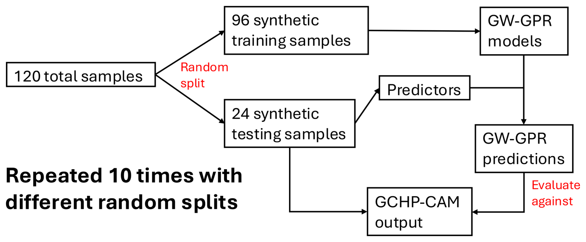
Figure 3 Schematic of the 10-fold random subsampling cross-validation procedure. At each “fold”, 80 % of the samples (96 runs) are used to train the emulator to predict the result from the other 20 % of the samples (24 runs). The prediction is then evaluated against the GCHP-CAM output ΔPM_2.5 for those 24 runs.

2.6 Testing the emulator with IGSM-GAINS-TAPS combined air quality and climate legislation scenarios

To evaluate the emulator within the context of integrated assessment modelling, we evaluate the ability of the emulator in reproducing GCHP-CAM output anthropogenic PM_2.5 over 2 climate (Current Trend (CT) and Accelerated Action (AA), both generated from MIT IGSM) (Paltsev et al., 2023) ×2 air pollution control – Current Legislation (CLE) and Maximum Feasible Reduction (MFR), in total 4 scenarios (CT_CLE, CT_MFR, AA_CLE, AA_MFR) in 2050 (Fig. 4). CT assumes the implementation of Nationally Determined Contributions (NDCs) from Paris Agreement through 2030. Under CT, climate is not stabilized, and global mean temperature continues to increase. AA assumes the extension of these initial NDCs to align with the long-term goal of Paris Agreement, providing the ability to limit and stabilize anthropogenic warming to 1.5 °C at 2100 with at least 50 % probability. The CLE scenario assumes complying with existing region- and source-specific air pollutant emission limits, while the MFR scenario assumes increasing deployments of currently available lowest-emitting technologies.

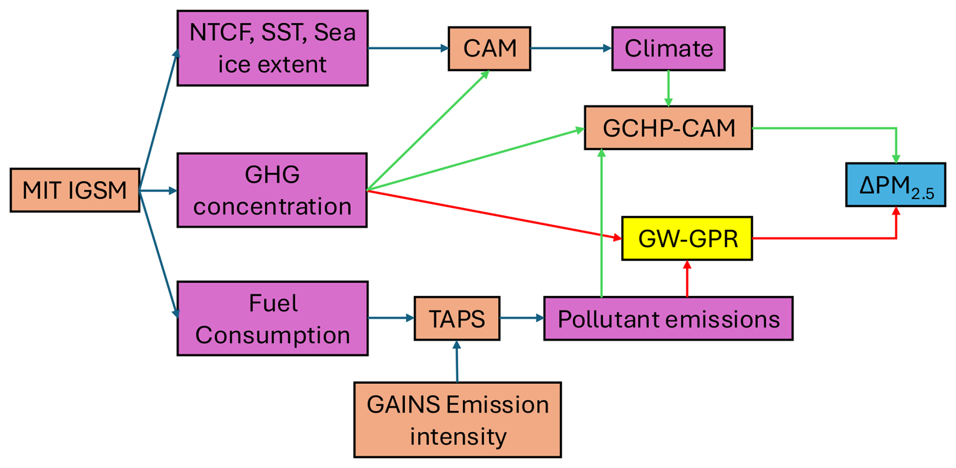
Figure 4 Schematic of GW-GPR model evaluation using IGSM-GAIN-TAPS climate and air pollution scenarios. Orange boxes represent existing modelling systems, purple boxes represent data sets. Yellow represents our newly developed emulator (GW-GPR). Green and red arrows represent how GCHP-CAM and GW-GPR predicts changes in PM_2.5, respectively.

The projected trends of air pollutant emission intensities under CLE and MFR scenarios are from Greenhouse gas-Air pollution INteractions and Synergies (GAINS) model (Amann et al., 2011), based on GAINS4/ECLIPSE (Evaluating the Climate and Air Quality Impacts of Short-lived Pollutants) v6b data (GAINS Developer Team, 2021; Klimont et al., 2017; Smith et al., 2020; Stohl et al., 2015). Future air pollutant emissions for each scenarios can be derived through the Tool for Air Pollution Scenarios (TAPS) (Atkinson et al., 2022a) by considering climate (fuel consumption) and air pollution (emission intensities) policies independently. The resulting regional (region definition shown in Fig. 5) and global air pollutant emissions of each of the 4 combined scenarios are shown in Fig. 6. The 4 scenarios have distinct emission scaling factors at each region, with less than 1 % of the region-scenario combinations having emission changes > 100 % (upper limit of training set). With these scenarios, we can test whether the emulator (trained on GCHP-CAM runs with globally uniform emission scaling factors) can perform reasonably under spatially heterogenous emission scaling factors, and within the intended range of emission changes.

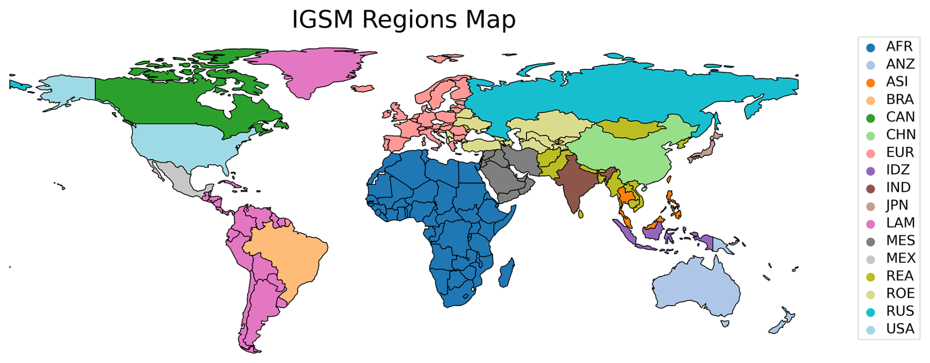
Figure 5 IGSM region definition.

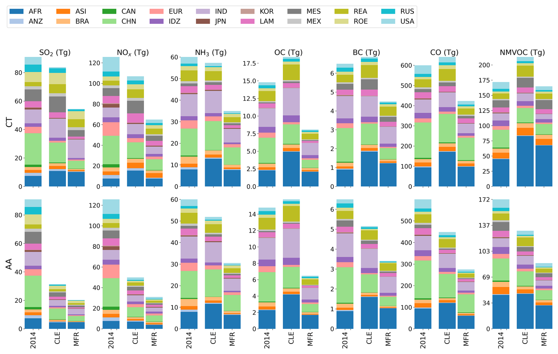
Figure 6 Total and regional air pollutant emissions for the four IGSM-GAINS-TAPS scenarios. Each row represents a climate scenario (Current Trend, CT; and Accelerated Actions, AA), and the emissions at 2014, and 2050 under Current LEgislation (CLE) and Maximum Feasible Reduction (MFR) air pollution control scenarios are shown for each species.

We perform 10 years of GCHP-CAM simulations for each of the four IGSM-GAINS-TAPS scenarios with their respective anthropogenic air pollutant emissions, and CH₄ and CO₂ concentrations in 2050. The simulations are driven by IGSM-CAM meteorological fields from the “REF” scenario, with meteorological years (2031–2041 for AA and 2040–2050 for CT) chosen to match the CO₂ concentration and TRF (i.e. AA has similar CO₂ concentration and TRF at 2050 with “REF” over 2031–2041, and CT has similar CO₂ concentration and TRF at 2050 with “REF” over 2040–2050). The same GCHP-CAM input anthropogenic air pollutant emissions, and CH₄ and CO₂ concentrations in 2050 are fed into the GW-GPR emulator to estimate ΔPM_2.5 under each scenario, which is then compared to the multiannual mean ΔPM_2.5 simulated by GCHP-CAM (Sect. 3.3).

2.7 Demonstrating the utility of the emulator using AerChemMIP data

To demonstrate the utility of the emulator, particularly under global change scenarios, we also compare the output of the GW-GPR emulator with the output from the Aerosol Chemistry Intercomparison Project (AerChemMIP) under 2 Shared Socio-economic Pathways (SSP)-based scenarios: (1) the standard SSP3-7.0 “Regional Rivalry” scenario (radiative forcing = 7.0 W m⁻² at 2100); and (2) a variant of SSP3-7.0 with same socio-economic assumptions as the standard SSP3-7.0, but stronger air quality control measures, resulting in lower emissions of Near Term Climate Forcers (SSP3-7.0-lowNTCF) (Fujimori et al., 2017). AerChemMIP (Collins et al., 2017) is endorsed by the Coupled-Model Intercomparison Project 6 (CMIP 6) to quantify the impacts of aerosols and chemically reactive gases on climate. There are minimum model complexity requirements (atmosphere-ocean general circulation model with tropospheric aerosols driven by pollutant emission fluxes) to participate in AerChemMIP ensemble.

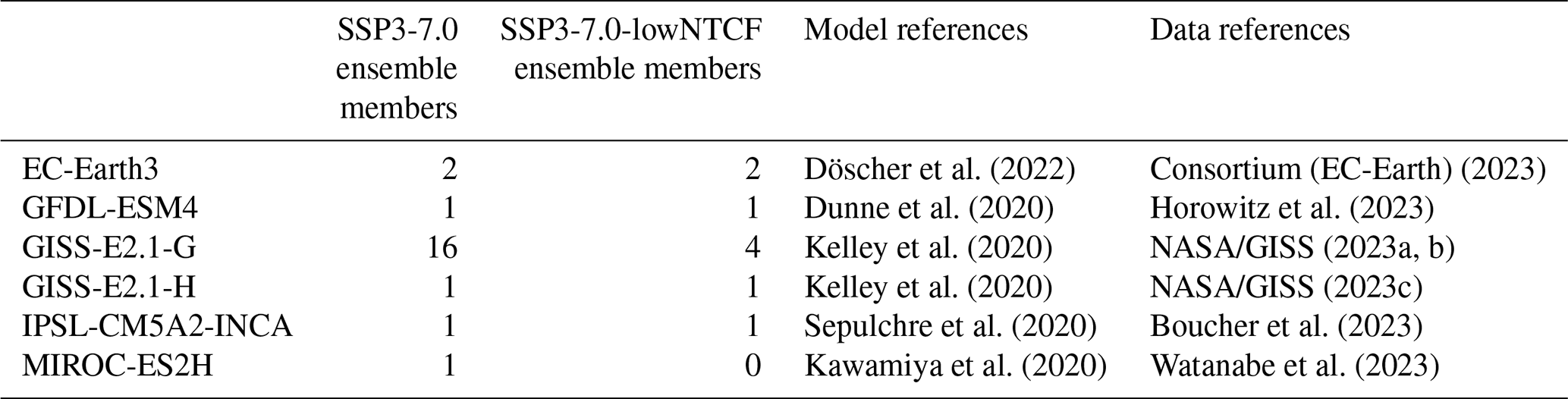
We calculate the anthropogenic PM_2.5 (sum of sulphate, nitrate, ammonium, BC and OC) from AerChemMIP archive in an identical manner as for GCHP-CAM (Eq. 2). We only include ensemble members with the output of all five anthropogenic PM_2.5 components available. The models selected and numbers of realizations included for each model are summarized in Table 2.

Table 2 The numbers of ensemble members with all 5 anthropogenic PM_2.5 components (sulphate, nitrate, ammonium, BC, OC) available for SSP3-7.0 and SSP3-7.0-lowNTCF scenarios from the AerChemMIP archive.

The emulator calculates the decadal changes in anthropogenic PM_2.5 concentrations relative to 2020 over 2030–2090, using surface air pollutant emissions (calculated as anthropogenic + open burning emissions) and GHG concentration (Meinshausen et al., 2020) provided by the Input4MIP repository. As air pollutant emissions are provided every 10 years, one emulator prediction is done per decade. For each ensemble member in the AerChemMIP archive, the corresponding decadal changes in anthropogenic PM_2.5 are calculated by comparing the decadal average anthropogenic PM_2.5 with that of the first decade (2015–2024). The model-specific decadal changes in anthropogenic PM_2.5 are then calculated by averaging the result from all the ensemble members from the corresponding model. AerChemMIP and Input4MIP data are retrieved via the search engine of Earth System Grid Federation (ESGF) (https://aims2.llnl.gov, last access: 26 August 2024). The comparison between emulator predicted and AerChemMIP output trends in anthropogenic PM_2.5 will be discussed in Sect. 4.

2.8 Health impact calculation

For the four climate and air pollution control scenarios, we also estimate the impacts of changes in anthropogenic PM_2.5 on public health through premature mortalities. GCHP and emulator output are upsampled from 2°×2.5° to 0.5°×0.5° using the nearest neighbour algorithm, which matches the horizontal resolution of the age-specific population data we use (Gridded Population of the World version 4.11, last access: 19 April 2024) (Center For International Earth Science Information Network-CIESIN-Columbia University, 2018). Country-scale baseline age- and cause-specific mortality rates are provided by the World Health Organization (WHO) (WHO, 2018). The age- and cause-specific changes in the annual mortality due to chronic PM_2.5 exposure for scenario i (ΔMort_i) is calculated from the relative mortality risks under the baseline (total PM_2.5 from the 2014 baseline run) (RR_base) and each scenario i (RR_i):

$$\begin{array}{}\text{(9)}& \mathrm{\Delta }{\mathrm{Mort}}_i={\mathrm{Mort}}_{\mathrm{base}}\left({\displaystyle \frac{{\mathrm{RR}}_i-{\mathrm{RR}}_{\mathrm{base}}}{{\mathrm{RR}}_{\mathrm{base}}}}\right)\end{array}$$

where Mort_base is the age- and cause-specific mortalities from the WHO.

We use the age-specific non-linear Concentration Response Functions from the Global Exposure Mortality Model (Burnett et al., 2018) to calculate RR_i and RR_base for non-communicable diseases and lower respiratory infections attributable to outdoor PM_2.5 pollution. Since our emulator focuses on the changes and corresponding impacts in anthropogenic PM_2.5, the synthetic PM_2.5 concentration for scenario i at each grid cell is calculated as PM${}_{\mathrm{2.5},\mathrm{base}}+\mathrm{\Delta }$PM_2.5,i, where PM_2.5,base is the modelled total PM_2.5 in year 2014, and ΔPM_2.5,i is the modelled/emulated change in anthropogenic PM_2.5 for scenario i.

3 Evaluation of the emulator

In this section we discuss and explain the performance of our GW-GPR emulators against GCHP-CAM simulations measured by the response of anthropogenic PM_2.5 pollution and associated premature mortalities.

3.1 Computing resource requirement

GCHP-CAM requires 2400–3000 CPU hours (Intel Xeon Processor E5-2679A v4, processor base frequency = 2.6 GHz) to simulate PM_2.5 for each 1-year run. The one-time operation of fitting the GW-GPR emulator requires 280 CPU hours (Intel Xeon Processor E5-2670, processor base frequency = 2.6 GHz). Once trained, the emulator requires approximately 10 CPU seconds to generate global PM_2.5 predictions for one scenario (Intel Xeon Processor Silver 4214R, processor base frequency = 2.4 GHz). This demonstrates the magnitude of the speed up offered by the emulator.

3.2 Emulator cross validation and sensitivity

In this sub section, we discuss the result of the cross validation and sensitivity test outline in Sect. 2.5. Figure 7 shows the result grid cell by grid cell comparison of changes in annual mean anthropogenic PM_2.5 (ΔPM_2.5) predicted by the GW-GPR emulator against that simulated by its parent model (GCHP-CAM) across all the data points generated by the random subsampling. The GW-GPR emulator can predict ΔPM_2.5 GCHP-CAM with reasonable accuracy (R²=0.97, mean absolute error (MAE) = 0.356 µg m⁻³) and minimal overall bias (mean bias (MB) = −0.012 µg m⁻³). Figure 8 shows the spatial distribution of grid cell scale MAE of the GW-GPR emulator, and the emulator output standard deviation from Eq. (4) (which can characterize the predictive uncertainty of emulator output). The largest MAE is found over Northern China and Northern India (up to 5 µg m⁻³), where the anthropogenic PM_2.5 and precursor emissions are very high in the base year of 2014. The emulator output standard deviation have similar magnitudes and spatial distributions (spatial R²=0.99) as MAE, confirming that emulator output standard deviation is an appropriate measure of the uncertainties of emulator predictions relative to the parent model.

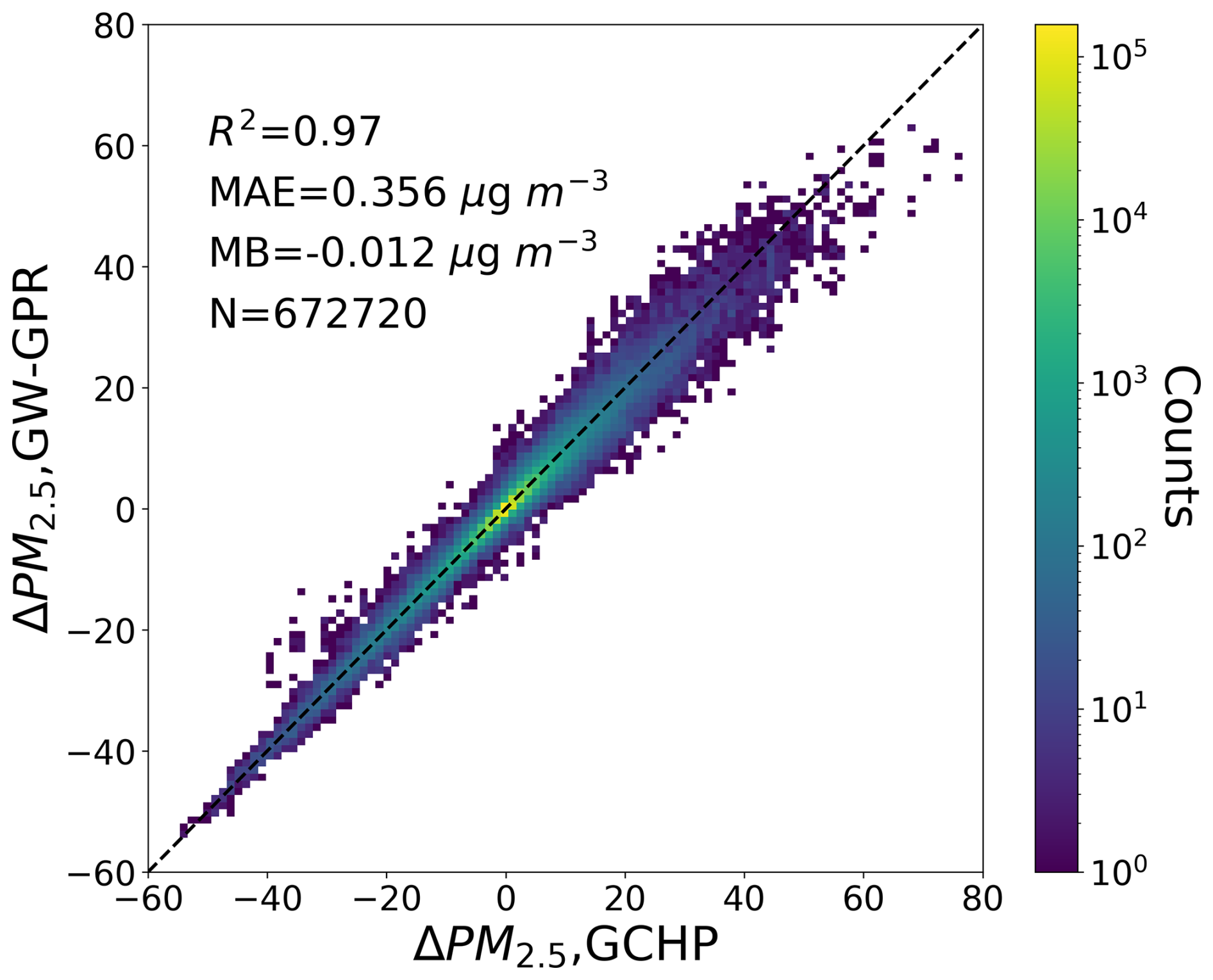
Figure 7 2D histogram from the grid cell by grid cell comparison between changes in annual mean anthropogenic PM_2.5 (ΔPM_2.5) predicted by the GW-GPR emulator (ΔPM_2.5, GW-GPR) and that simulated by GCHP-CAM (ΔPM_2.5, GCHP) from the 10-fold random sub-sampling cross-validation.

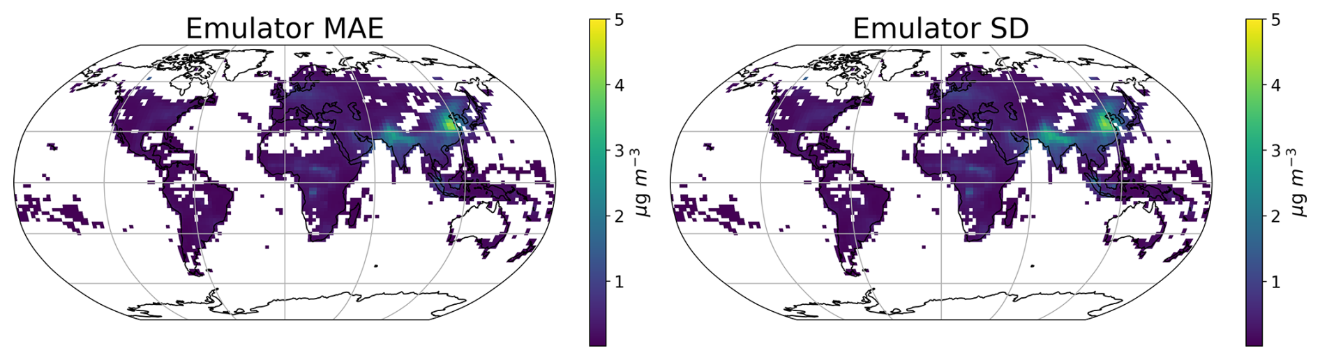
Figure 8 The mean absolute error (MAE) of emulator prediction against the parent model (GCHP-CAM), and the average standard deviation of emulator predictions from Eq. (4) (indicative of predictive uncertainties) at grid cell scale (240 data points at each grid cell).

Figure 9 shows the normalized Sobol Total Sensitivity Indices of the GW-GPW emulator to each of the input variables (in the unit of fractional rather than absolute changes), which measure how much each input variable is responsible for the variance in the output over the whole domain of input data, including the interaction among variables. In other words, the Sensitivity Indices indicate how important the specific input variable is in controlling the output. The importance of input variables is spatially heterogenous. Over North America and Europe, ΔPM_2.5 is mostly sensitive to SO₂ (46 %–57 % of total sensitivity index) and NH₃ (28 %–32 %), and to a lesser extent NO emissions (10 %–14 %). The pattern of total sensitivity indices over India and China are similar (9 %–13 % for NO, 21 %–37 % for NH₃ and 36 %–57 % for SO₂), but the sensitivity of ΔPM_2.5 to OC (13 % vs. 3 %–7 % over North America and Europe) is higher over these regions. For most of the rest of the northern hemisphere, ΔPM_2.5 is primarily sensitive to SO₂ emissions (e.g. >80 % over Mexico and Middle East). Over the southern hemisphere, ΔPM_2.5 remains highly sensitive to SO₂ emissions (47 % over Indonesia – 76 % over Brazil). In Brazil, Indonesia, and Africa, ΔPM_2.5 is also sensitive to OC emissions (15 %–38 %). Sensitivity of ΔPM_2.5 to BC is relatively low globally (mean = 0.006 over the globe). This is because BC is largely co-emitted with OC, while the OC emissions are always around 1–2 times larger than BC emission by mass. Thus, the variance attributable to BC is mostly captured by the variance attributable to OC. The sensitivity index of CO₂, CH₄, VOC and CO are also relatively low (<3 %) globally, except over the certain regions with low anthropogenic emissions (tropical Pacific islands, edge of the Amazon and central African rainforests), reflecting the fact that our emulator does not consider SOA in our definition of anthropogenic PM_2.5.

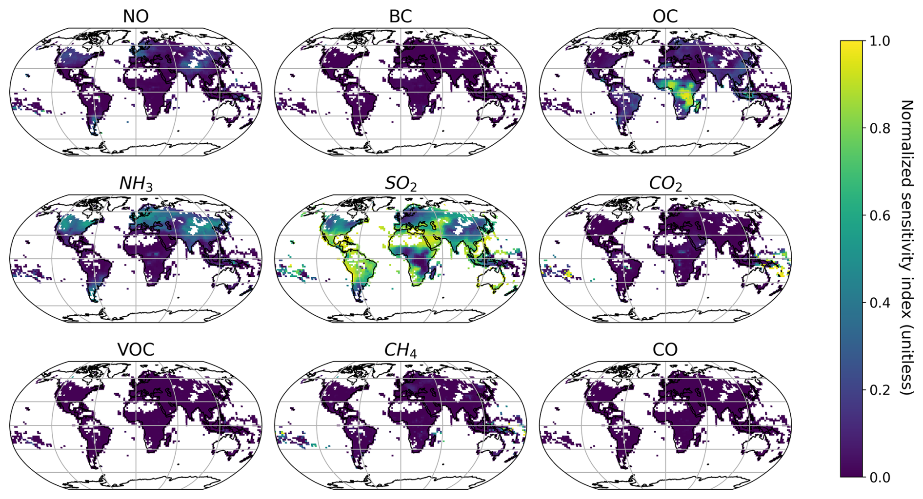
Figure 9 Spatial patterns of Sobol Total Sensitivity Indices (0–1) for each predictor for ΔPM_2.5. The indices indicate the fraction of output variance attributable to each input variables at each grid cell.

3.3 Comparing emulator performance for IGSM-GAINS-TAPS scenarios with GCHP-CAM

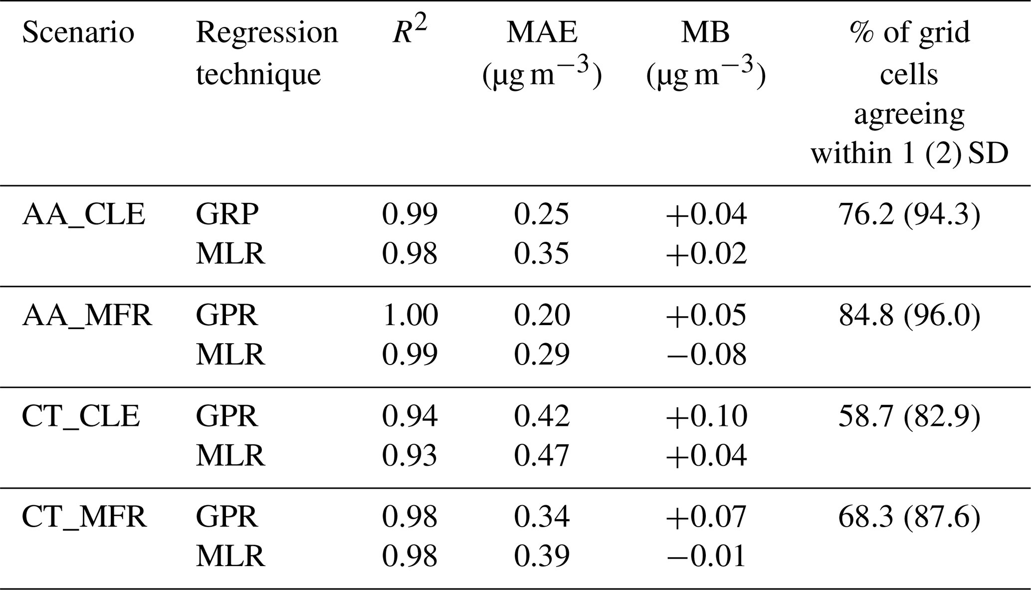
Figure 10 shows the GCHP-CAM and GW-GPR (emulator) output ΔPM_2.5 (2045–2054 mean vs. 2014) over each IGSM-GAINS-TAPS scenario at grid cell scale. The global performance metrics are shown in Table 3. Generally, the emulator performs comparably to that in the random subsampling evaluation (R²=0.94–0.99, MAE = 0.20–0.42 µg m⁻³). 58.7 % (82.9 %)–84.8 % (96 %) of the grid cells have emulator predictions agreeing with GCHP-CAM within 1 (2) standard deviation of emulator output respectively (computed with Eq. 5).

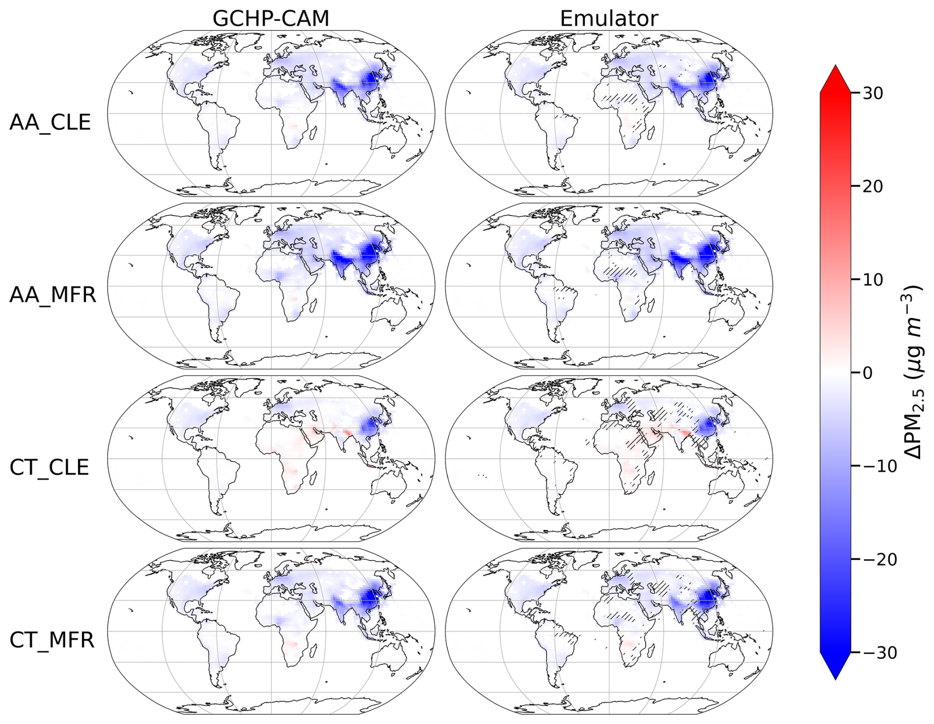
Figure 10 Spatial patterns of GCHP-CAM and emulator predicted ΔPM_2.5 for each of the 4 IGSM-GAINS-TAPS scenarios at 2050 (relative to 2014). Only results in grid cells with population density > 1 person per km² are shown. The hatches show where GCHP-CAM output does not fall within the 95 % confidence interval of emulator prediction.

Table 3 Gaussian Process Regression (GPR) and multilinear regression (MLR) emulator performance metrics (spatial coefficient of determination (R²), mean absolute error (MAE), mean bias (MB), computed at grid cell scale, N=2803) for each IGSM-GAINS-TAPS scenarios, relative to GCHP-CAM output. The rightmost column indicates the percentage of grid cells that the GPR emulator prediction agrees with GCHP-CAM output within 1 (2) standard deviation (prediction uncertainty of emulator).

When the predicted spatial distributions of ΔPM_2.5 are converted into premature mortalities using the GEMM CRF, we find that the GCHP-CAM and emulator output produce similar impacts on global premature mortalities over the 4 IGSM-GAINS-TAPS scenarios tested (differences within 1.2 %) that agree within the range of uncertainty due to the GEMM CRF parameters (Fig. 11). This shows the emulator's ability to reproduce both the magnitudes and spatial distributions of ΔPM_2.5 from GCHP-CAM, and the suitability of emulator output for public health impact calculation at global scale.

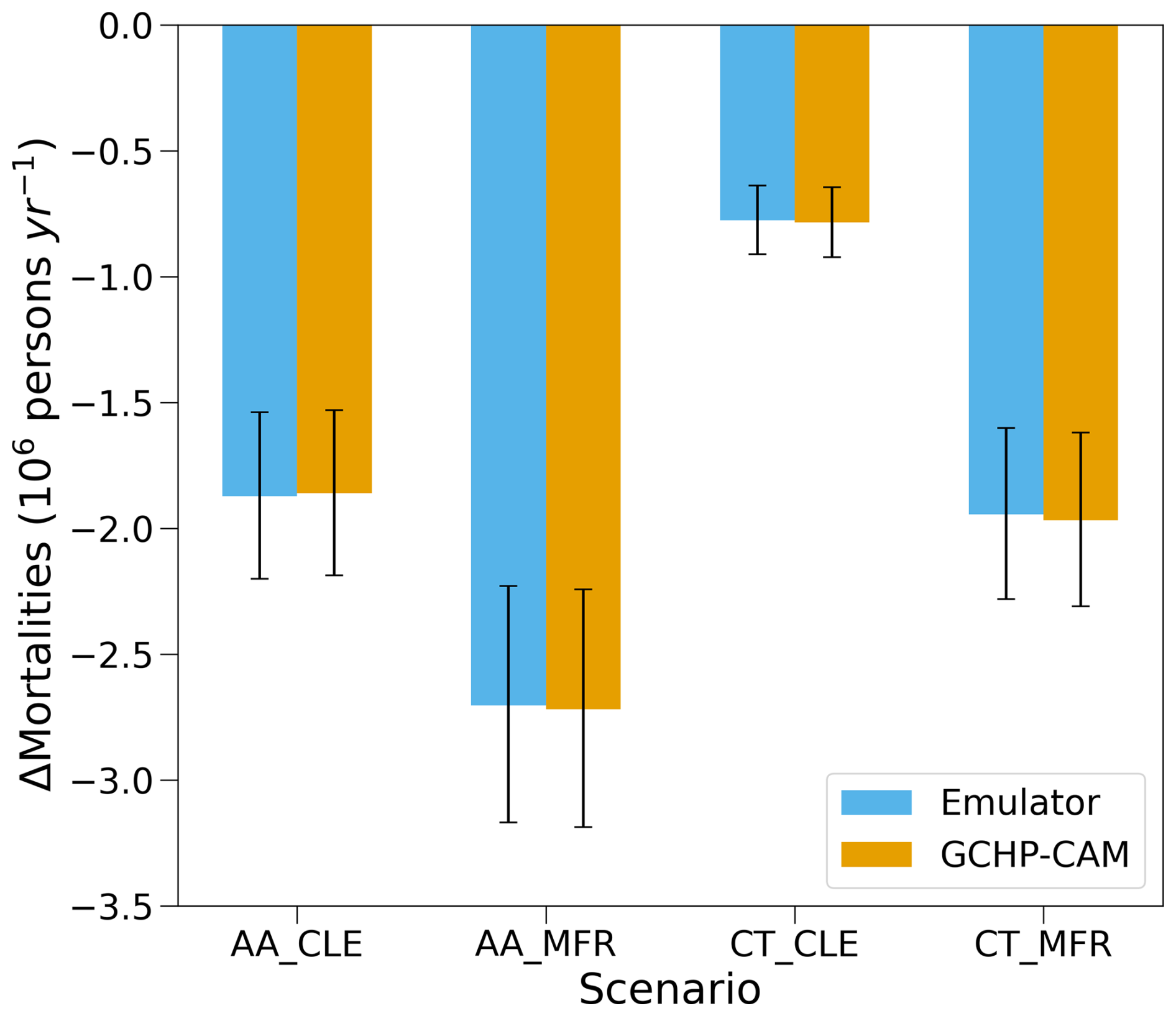
Figure 11 Changes in global annual premature mortality attributable to PM_2.5 exposure under each of the four scenarios between 2050 and 2014, calculated from the emulator and GCHP-Chem output ΔPM_2.5. The error bars represent the uncertainties due to GEMM CRF parameters, calculating by applying the 2.5 and 97.5 percentile estimate of the GEMM CRF parameters.

In general, the emulator performs best over the western hemisphere (longitude < −20°), where the emulator error is within 2 µg m⁻³ (MAE = 0.1 µg m⁻³), and 77.4 % of emulator predictions agree with GCHP-CAM output within 1 emulator output standard deviation. In contrast, the emulator output shows consistent high bias of up to 2 µg m⁻³ over the 4 scenarios over the Sahel. Around the Bay of Bengal, emulator output does not agree with GCHP-CAM output with 1 emulator output standard deviation in a large portion of grid cells. In the subsections below, we will explore the potential sources of error by comparing the result presented above with that from alternative emulator architectures.

3.3.1 Comparison with linear model

For comparison, we train a multilinear regression (MLR) emulator with identical variables, geographic weighting and normalization schemes, and the performance metrics of the multilinear emulator is also shown in Table 3. In all scenarios, the MLR estimator has a larger global MAE than GPR (by 0.05 µg m⁻³ (19 %) in CT_CLE to 0.10 µg m⁻³ (40 %) in AA_CLE). However, in 3 out of 4 scenarios tested (except AA_MFR), the GPR emulator has higher MB than the MLR emulator, though the overall magnitudes of MB remain relatively small (within 0.1 µg m⁻³).

Figure 12 shows the spatial distribution of MLR and GPR error relative to their parent model (GCHP-CAM), and Fig. 13 shows the difference in absolute values of such errors between MLR and GPR. In the 4 IGSM-GAINS-TAPS scenarios, GPR predictions have less absolute error relative to the parent model than MLR in 57.6 % (CT_CLE) to 66.4 % (AA_MFR) of the grid cells. In all 4 scenarios, GPR outperforms MLR over the US (MAE = 0.05–0.14 µg m⁻³ for GPR vs. 0.17–0.29 µg m⁻³ for MLR), western and southern Europe (MAE = 0.05–0.06 µg m⁻³ for GPR vs. 0.20–0.26 µg m⁻³ for MLR), Middle East (MAE = 0.16–0.56 µg m⁻³ for GPR vs. 0.40–0.72 µg m⁻³ for MLR), South America (MAE = 0.08–0.14 µg m⁻³ for GPR vs. 0.14–0.16 µg m⁻³ for MLR), and South Asia.

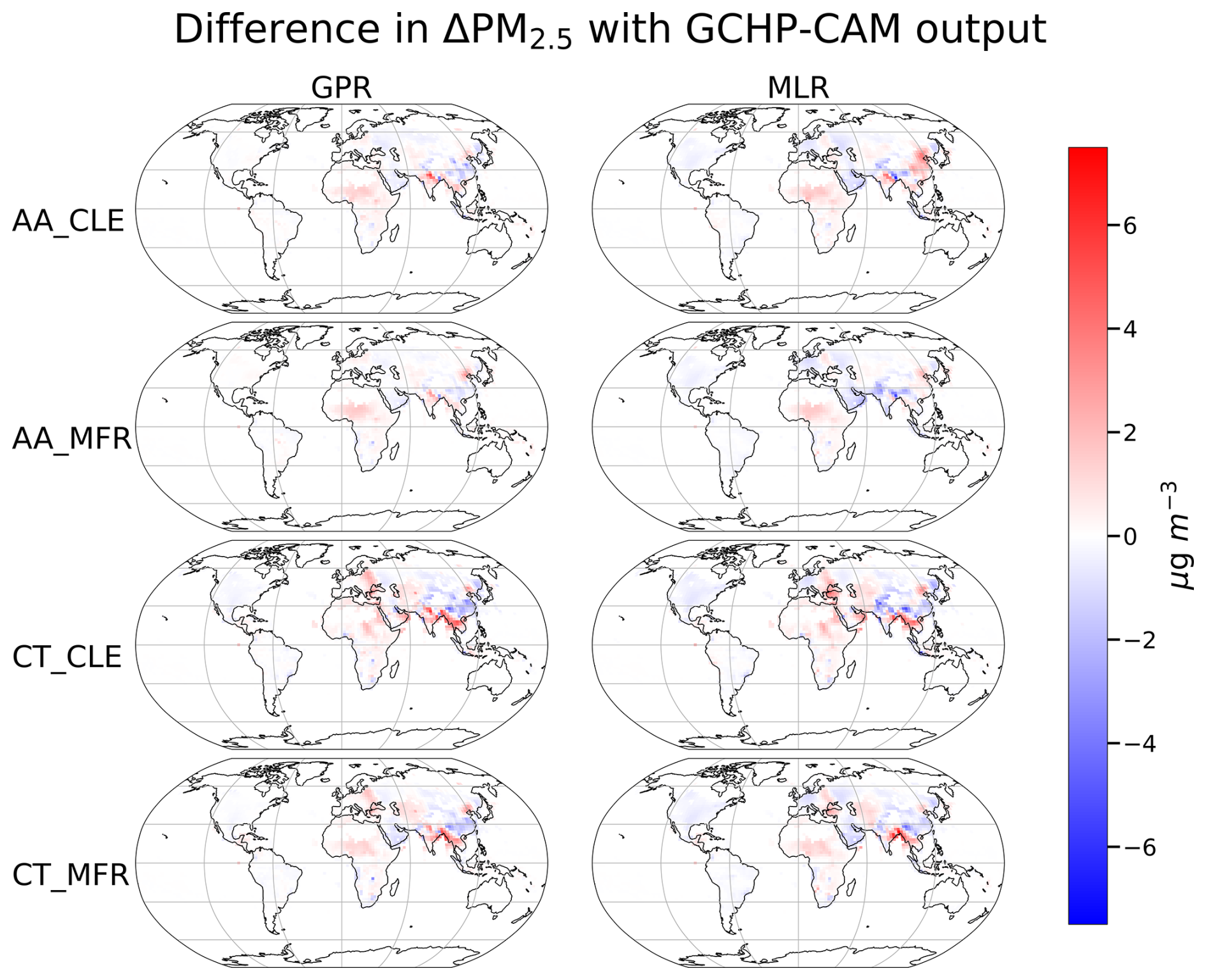
Figure 12 GPR and MLR emulator errors relative to GCHP-CAM simulated ΔPM_2.5 over the 4 IGSM-GAINS-TAPS scenarios at 2050 (relative to 2014). Both emulators use the same geographic weighting scheme for pollutant emissions.

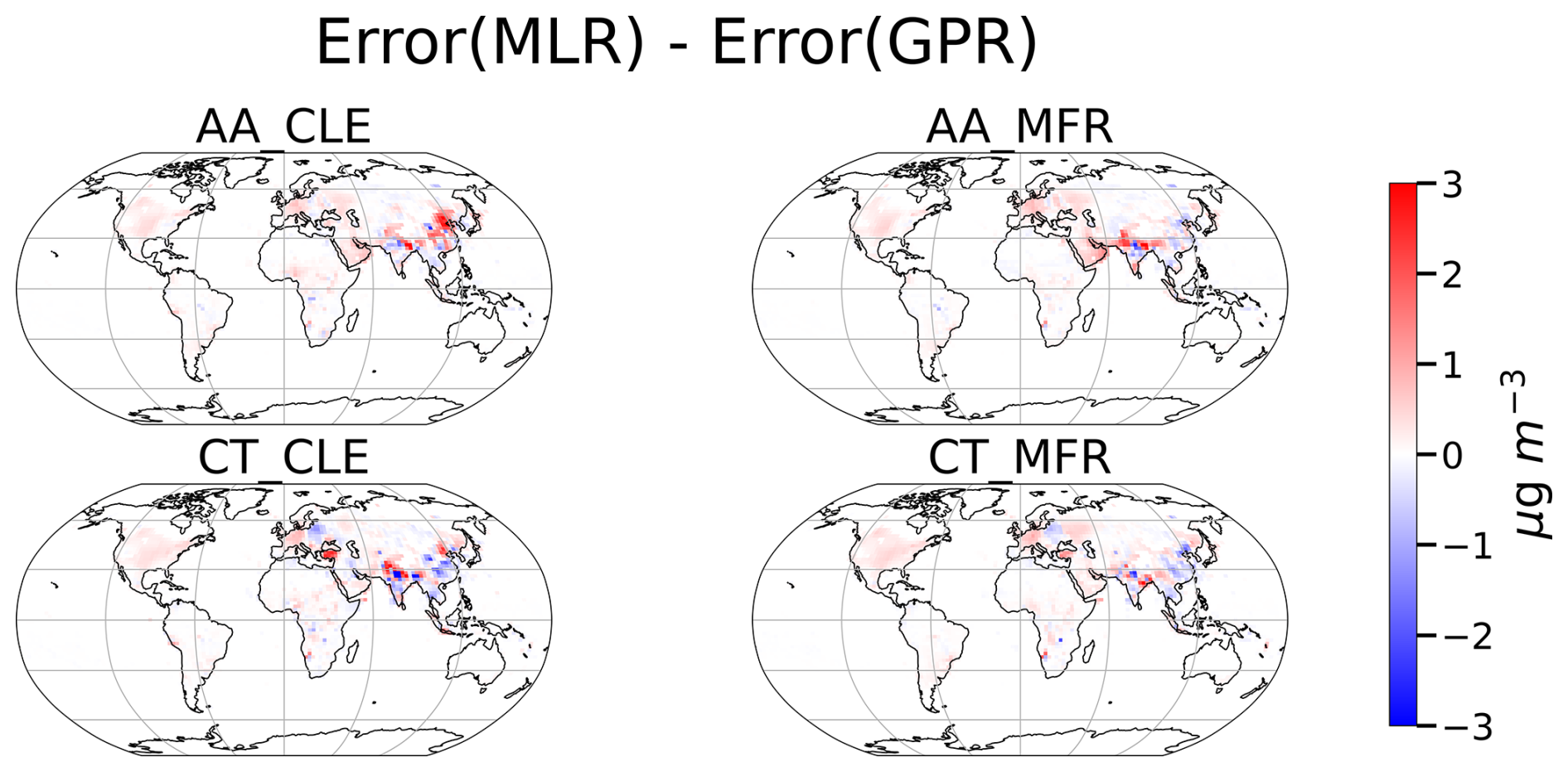
Figure 13 Difference in the absolute error (relative to GCHP-CAM output) between MLR and GPR emulation. Red (positive) indicate GPR is more accurate than MLR at the given grid cell, while blue (negative) indicates the opposite.

To further understand the utility of non-linear emulation, we analyse the shifts in the chemical regime of secondary inorganic aerosol formation calculating the Gas Ratio (GR) (Paulot and Jacob, 2014) over China at baseline year and under all 4 scenarios (Fig. 14):

$$\begin{array}{}\text{(10)}& \mathrm{GR}={\displaystyle \frac{\left[{\mathrm{NH}}_{\mathrm{3}}\right]+\left[{\mathrm{NH}}_{\mathrm{4}}^{+}\right]-\mathrm{2}\left[{\mathrm{SO}}_{\mathrm{4}}^{\mathrm{2}-}\right]}{\left[{\mathrm{HNO}}_{\mathrm{3}}\right]+\left[{\mathrm{NO}}_{\mathrm{3}}^{+}\right]}}.\end{array}$$

GR < 0 indicates that secondary inorganic PM_2.5 is weakly sensitive to NH₃ emissions through adding NH${}_{\mathrm{4}}^{+}$ to existing SO${}_{\mathrm{4}}^{\mathrm{2}-}$ and HSO${}_{\mathrm{4}}^{-}$ ions. 0 < GR < 1 indicates that there is enough NH₃ to react with SO${}_{\mathrm{4}}^{\mathrm{2}-}$, such that NH₃ and HNO₃ start partitioning into NH₄NO₃ aerosol, leading to strong sensitivity of secondary inorganic PM_2.5 to NH₃ emissions. In this regime, secondary inorganic PM_2.5 is more sensitive to NH₃ emissions. GR > 1 indicates that there is more than enough NH₃ to react with both SO${}_{\mathrm{4}}^{\mathrm{2}-}$ and HNO₃, and PM_2.5 sensitivity to NH₃ emissions will weaken continuously as GR keep increasing beyond 1 (Ansari and Pandis, 1998).

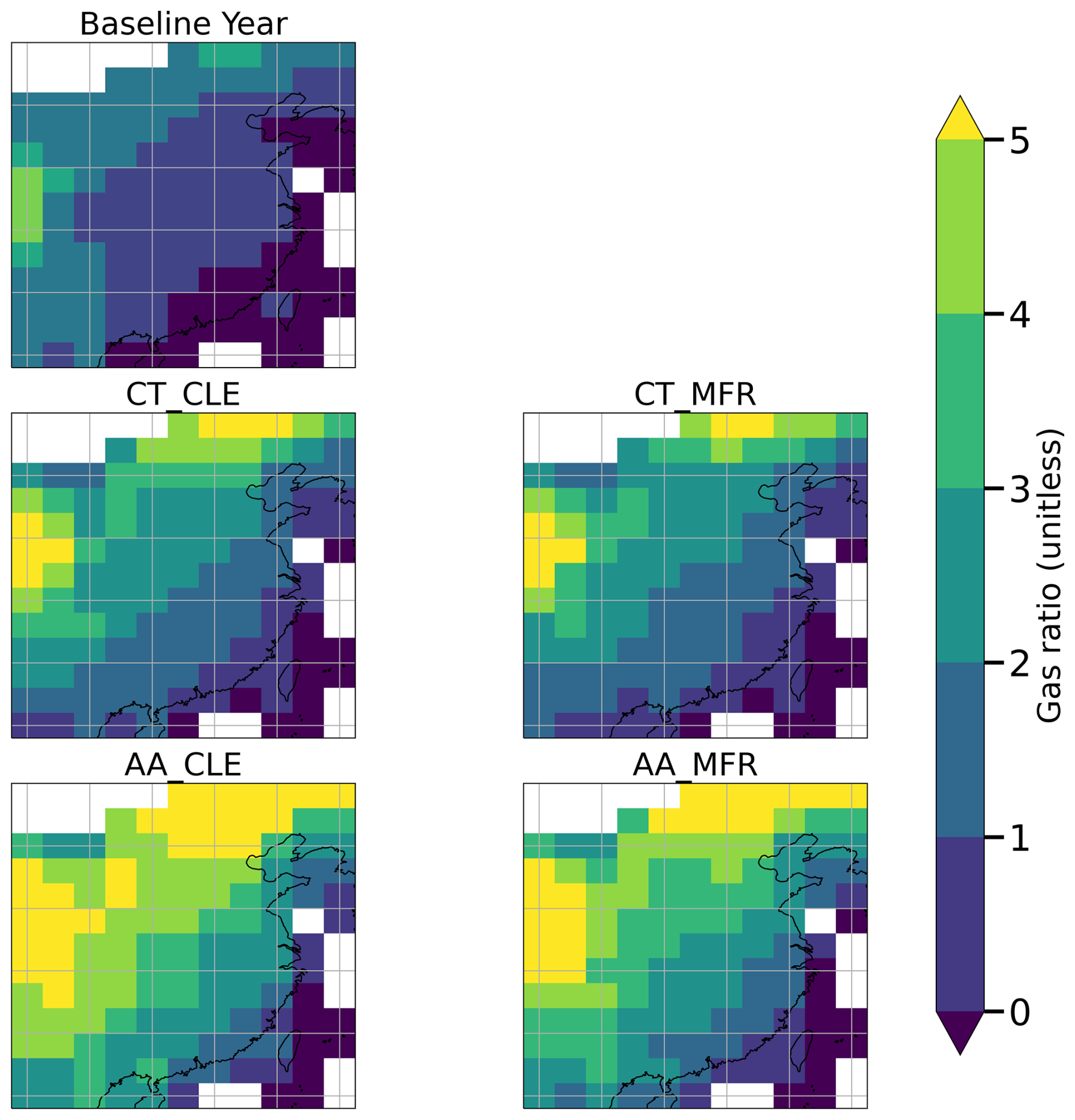
Figure 14 Gas ratio (GR) over China, which indicate secondary inorganic PM_2.5 sensitivity to NH₃ emissions. Secondary inorganic PM_2.5 is weakly sensitive to NH₃ when GR < 0.0 < GR < 1 indicate stronger sensitivity of secondary inorganic PM_2.5 to NH₃ emissions. When GR > 1, sensitivity of secondary inorganic PM_2.5 to NH₃ emissions decreases as GR increases.

In northern China, GPR is slightly less accurate than MLR on average under the MFR scenarios (by 0.31 µg m⁻³ under AA_MFR and 0.38 µg m⁻³ under CT_MFR, measured by regional MAE), but considerably more accurate under CLE scenarios (by 2.01 µg m⁻³ under AA_CLE and 0.81 µg m⁻³ under CT_CLE). At the baseline year, GR over Northern China is largely between 0–1. Under all four scenarios, GR increases beyond 1 over northern China. However, the increases in GR are the strongest under AA_CLE, followed by AA_MFR, while CT_CLE and CT_MFR have lower GR than the two AA scenarios. This indicates stronger shifts in secondary inorganic PM_2.5 sensitivity to precursor emissions relative to the baseline year (and therefore more non-linearity) under the two AA scenarios (especially AA_CLE) than the two CT scenarios, which is more well-captured by GPR than MLR.

The results in this sub-section show that GPR generally outperforms MLR. When emission changes could potentially trigger non-linear aerosol chemistry, non-linear emulators can be significantly more accurate than linear emulators. This justifies the use of non-linear regression techniques (e.g. GPR) in developing air quality emulators, especially given that GPR only requires 25 % more runtime than MLR.

3.3.2 Sensitivity to dispersion length scales (L)

In addition to regression techniques, we also conduct 4 sensitivity tests of altering the dispersion length scales for individual pollutants i (L_i): (1) L_i=0 (no geographic weighting); (2) halving L_i, (3) doubling L_i, (4) directly using atmospheric lifetime of pollutant to approximate L_i. Figure 15 shows the changes in absolute error of emulator prediction when the geographic weighting scheme is disabled (i.e. L_i=0). Turning off the geographic weighting scheme worsens the performance of the emulator, increasing the global MAE by between 0.31 µg m⁻³ (AA_MFR) and 0.88 µg m⁻³ (CT_CLE), and locally absolute error by up to 29.1 µg m⁻³. This decline in model performance is much larger than that by switching from GPR to MLR, indicating the necessity of the geographic weighting scheme in our emulator.

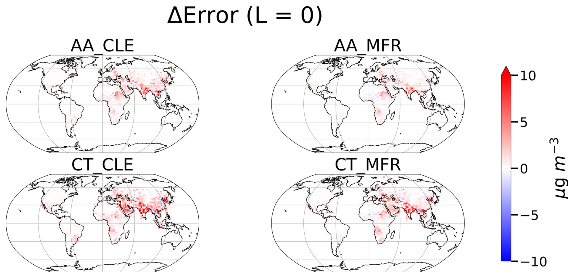
Figure 15 Changes in absolute error (relative to GCHP-CAM output ΔPM_2.5) when no geographic weighting of pollutant emissions is implemented. Red (positive) indicates that turning off dispersion worsens the performance (increasing error), blue (negative) indicates the opposite.

Figure 16 shows the changes in absolute error of emulator predictions when L_i are halved. Halving L_i increases global MAE at all the scenarios by 0.05 µg m⁻³ (AA_MFR) to 0.21 µg m⁻³ (CT_CLE), especially over the Sahel and northern India, where absolute error increases by up to 13.2 µg m⁻³. Figure 17 shows changes in absolute error of emulator predictions when L_i are doubled. Doubling L_i leads to minor changes in global MAE across the 4 scenarios (−0.015 µg m⁻³ under CT_CLE to +0.015 µg m⁻³ under CT_MFR). The geographic pattern of emulator performance changes is similar across different scenarios. After doubling the dispersion length scale, the emulator performs better over the Sahel, China and Indochina by up to 4.8 µg m⁻³ locally, but worse over India, where the regional MAE increases by 0.28 µg m⁻³ (AA_MFR) to 1.01 µg m⁻³ (CT_CLE), and local error increases by up to 4.05 to 9.67 µg m⁻³ over the 4 scenarios.

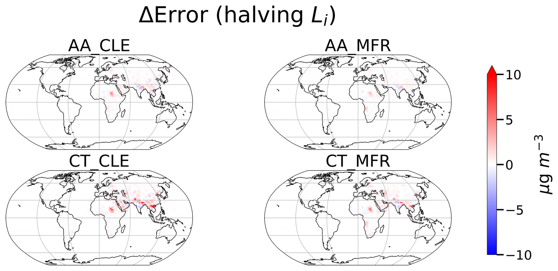
Figure 16 Changes in absolute error (relative to GCHP-CAM output ΔPM_2.5) when the dispersion length scales (L_i in Eq. 7) for all pollutants in the geographic weighing scheme are halved. Red (positive) indicates that turning off dispersion worsens the performance (increasing error), blue (negative) indicates the opposite.

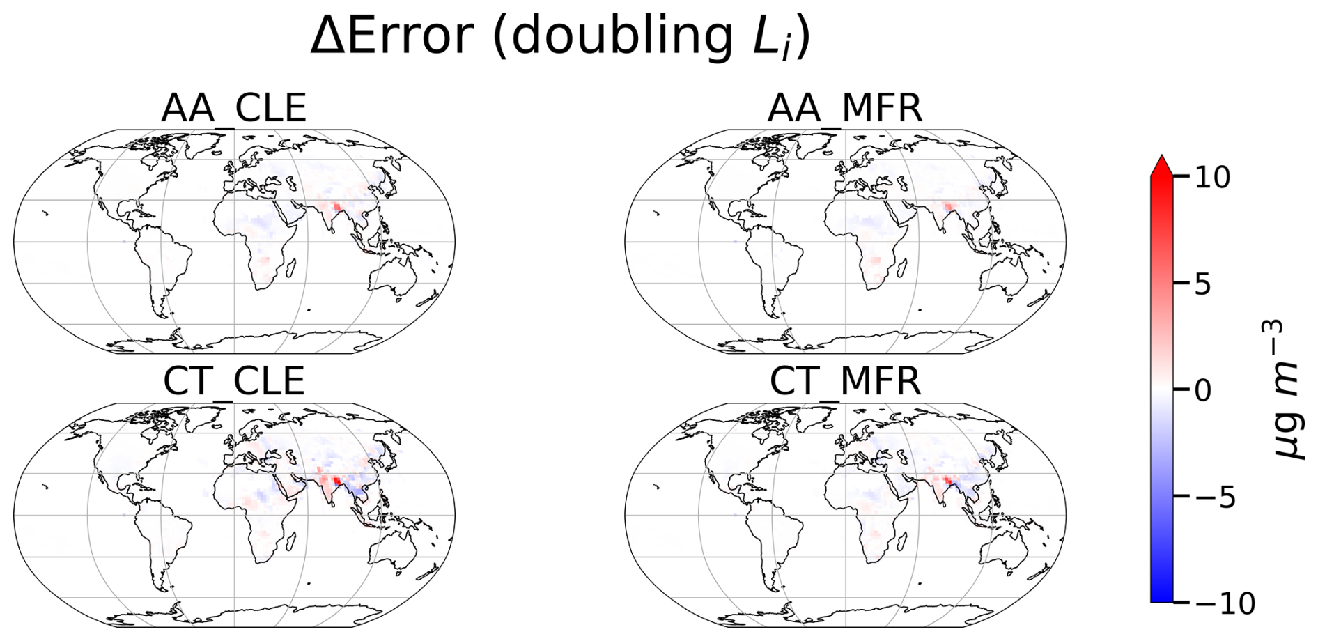
Figure 17 Changes in absolute error (relative to GCHP-CAM output ΔPM_2.5) when the dispersion length scales (L_i in Eq. 7) for all pollutants in the geographic weighing scheme are doubled. Red (positive) indicates that turning off dispersion worsens the performance (increasing error), blue (negative) indicates the opposite.

In the final sensitivity experiment, we assume L_i (in km) to be approximately equal to 10–20× atmospheric lifetime of pollutant i (τ_i) (Li and Cohen, 2021). Anthropogenic NO_x and NH₃ have very short τ (within a few hours) (Dammers et al., 2019; Lange et al., 2022). Also, HNO₃ (the main oxidized form of NO_x) (Muller et al., 1993) and NH₃ (Schrader and Brümmer, 2014) deposit rapidly. However, the secondary inorganic aerosol formed from anthropogenic NO_x and NH₃ have longer τ (3–5 d) (Bian et al., 2017). Balancing these two factors, we assume $L_{{\mathrm{NO}}_x}$ and $L_{{\mathrm{NH}}_{\mathrm{3}}}=\mathrm{1}$ grid cell. SO₂ has longer τ (4–12 h for point sources (Fioletov et al., 2015), and 1–1.5 d at regional and global scale (Chen et al., 2025; Hardacre et al., 2021; Lee et al., 2011)) and lower deposition velocity (Hardacre et al., 2021) than NO_x and NH₃. Therefore, we assume $L_{{\mathrm{SO}}_{\mathrm{2}}}=\mathrm{3}$ grid cells. Anthropogenic NMVOC that has the most significant contribution to photochemistry and oxidation chemistry (e.g. xylene, toluene, ethylene, propylene) (Gu et al., 2021; Ran et al., 2011) typically have τ of a few hours to 2 d (Franco et al., 2022; Tiwari et al., 2010; Trentmann et al., 2003). Therefore, we assume L_VOC=2 grid cells. As recent studies suggests that τ_BC<5 d (Lund et al., 2018), and τ_BC≈τ_OC (Gao et al., 2022), we assume of $L_{\mathrm{BC}}=L_{\mathrm{OC}}=\mathrm{7}$ grid cells. As τ_CO is at the order of months (Khalil and Rasmussen, 1990), we choose L_CO=15 grid cells to avoid excess processing time by the geographic weighting scheme.

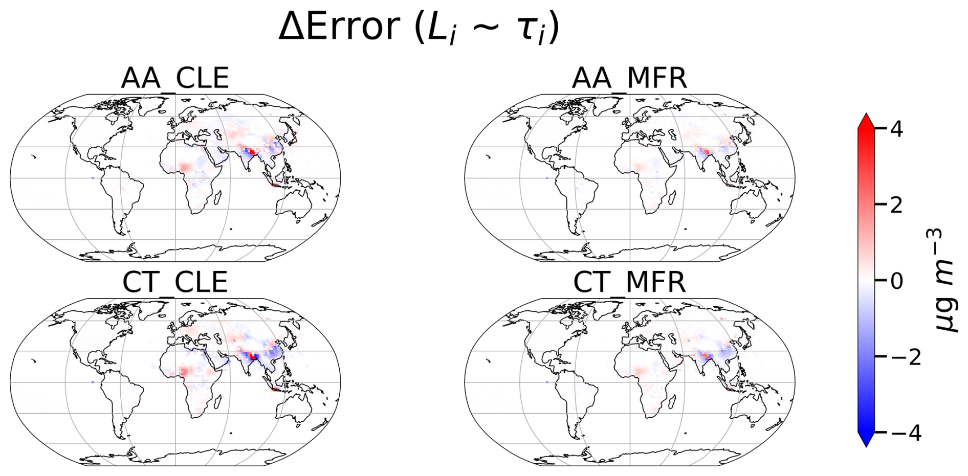
Figure 18 Changes in absolute error (relative to GCHP-CAM output ΔPM_2.5) when an alternate set of L_i ($L_{{\mathrm{NH}}_{\mathrm{3}}}=L_{{\mathrm{NO}}_x}=\mathrm{1}$ grid cell, L_VOC=2 grid cells, $L_{{\mathrm{SO}}_{\mathrm{2}}}=\mathrm{3}$ grid cells, $L_{\mathrm{BC}}=L_{\mathrm{OC}}=\mathrm{7}$ grid cells, L_CO=15 grid cells, informed by the atmospheric lifetime of each pollutant i (τ_i)) is applied to train the GW-GPR. Red (positive) indicates that using the alternate set of L_i worsens the performance (increasing error), blue (negative) indicates the opposite.

Figure 18 shows the changes in absolute error of emulator predictions with the set of L_i described above. The global performance metrics (MAE = 0.21–0.42 µg m⁻³, MB = 0.06–0.1 µg m⁻³) are very similar to the metrics obtained by training the GW-GPR emulation with the default set of L_i. The regional pattern of changes in emulator accuracy is consistent over the 4 scenarios tested. Using this alternate set of L_i reduces the error over southern China by up to 4 µg m⁻³, while increasing the error over western Africa and central Asia by up to 4 µg m⁻³. Over northern India and Bangladesh, the emulator error could locally increase or decrease by up to 5 µg m⁻³. However, the generally larger L_i increases the runtime of the geographic weighting scheme (around 15 s), while only 0.6 s is required to run the geographic weighting scheme using our default choice of L_i. Given the GW-GPR emulator can finish its prediction within 10 s for each scenario, such a large increase in runtime without consistent global improvement in emulator performance is not justified.

The results of these sensitivity tests illustrate that the accuracy of our emulator is sensitive to the choice of L_i. While our choice of a set of globally uniform set of L_i provides a reasonable first-order approximation to emulate pollutant dispersion, performance of the emulator could conceivably be improved by regional, or even grid cell specific L_i. However, this will greatly increase the computing power required to train the model, and potentially require many additional global change scenarios to train and benchmark the model.

4 Evaluating utility: comparison with AerChemMIP ensemble

Figure 19 shows the changes in global population-weighted average anthropogenic PM_2.5 simulated by the models in the AerChemMIP ensemble and GW-GPR emulator over 2030–2090 under SSP3-7.0 and SSP3-7.0-lowNTCF scenarios, relative to the 2015–2024 average. The solid lines represent the mean predictions, and the shaded areas represent the ranges of uncertainty (min/max for AerChemMIP ensemble, 1 standard deviation for emulator). Global population-weighted average ΔPM_2.5 from the emulator is within the range of AerChemMIP ensemble for both SSP3-7.0 and SSP3-7.0-lowNTCF scenarios over 2030–2090. The emulator predicted decadal mean global population-weighted average ΔPM_2.5 falls well within the range and differs by less than 1.15 µg m⁻³ with the mean of AerChemMIP ensemble for all decades under both scenarios.

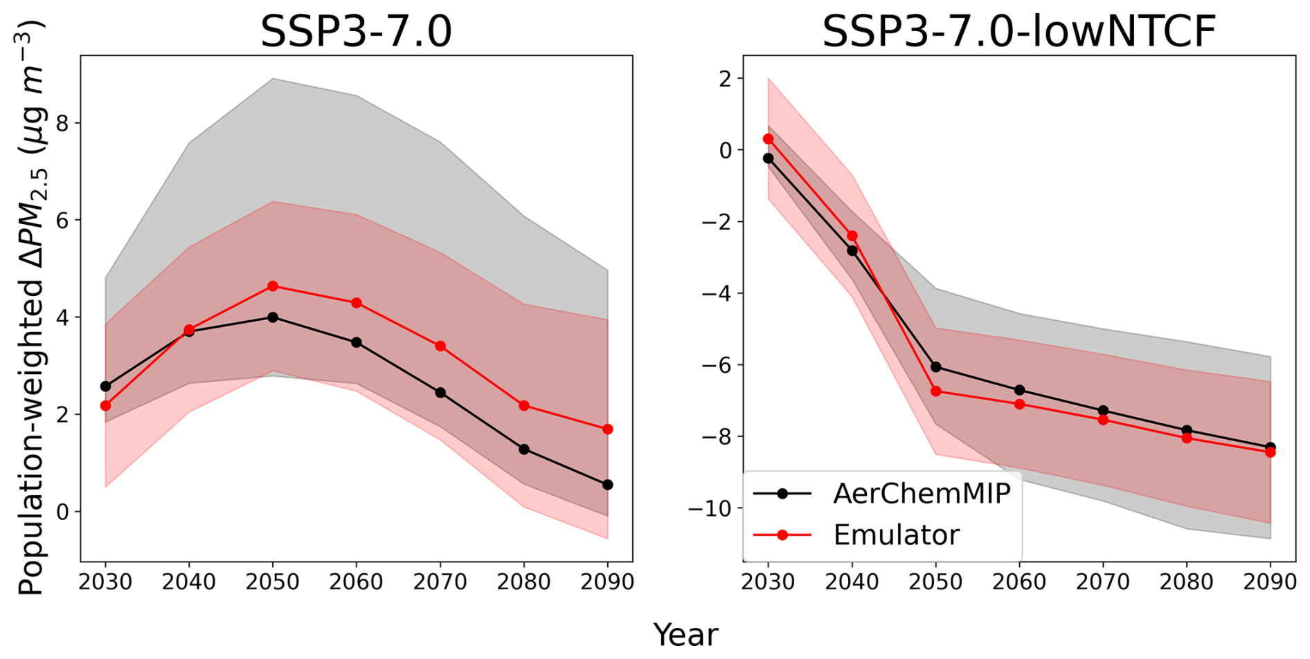
Figure 19 Changes in global decadal mean population-weighted anthropogenic PM_2.5 relative to 2015–2024 mean, predicted by the models in AerChemMIP ensemble and emulator with the shades indicate the range of uncertainty (ensemble range for AerChemMIP, 1 standard deviation for emulator), under standard SSP3-7.0 and the SSP3-7.0 low Near-Term Climate Forcer (SSP3-7.0-lowNTCF) scenario.

Figure 20 shows the multimodel minimum and maximum ΔPM_2.5 simulated by models in AerChemMIP and GW-GPR emulator predicted ΔPM_2.5 in 2050 and 2090 under SSP3-7.0 and SSP3-7.0-lowNTCF scenarios. Output from models in AerChemMIP is conservatively regridded to the same horizontal resolution for comparison. GW-GPR produces similar spatial patterns of ΔPM_2.5 as AerChemMIP models (e.g. large increases and decreases in PM_2.5 over northern China and northern India) in all four scenario-year combinations shown. Over major population centres in the northern Hemisphere (eastern North America, Europe, northern India), GW-GPR emulator predictions of ΔPM_2.5 largely fall within the range of AerChemMIP model output. This contributes to the agreement of global population-weighted average ΔPM_2.5 between GW-GPR emulator and models in AerChemMIP (Fig. 19).

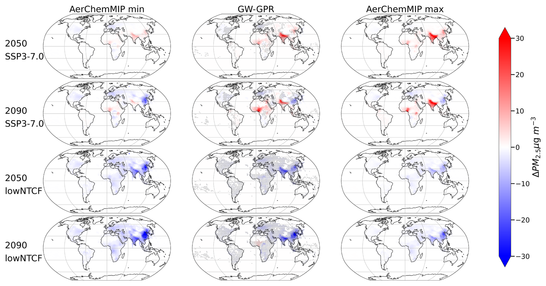
Figure 20 Multimodel minimum and maximum magnitude of ΔPM_2.5 simulated by models in AerChemMIP, and GW-GPR emulator predicted ΔPM_2.5 in 2050 and 2090 under SSP3-7.0 and SSP3-7.0-lowNTCF (abbreviated as lowNTCF in plot labels). Dots in the middle (GW-GPR) column indicate the grid cells where prediction of GW-GPR do not fall between the minimum and maximum of AerChemMIP simulation output.

However, there is systematic disagreement between GW-GPR and AerChemMIP model output over western Africa. Under SSP3-7.0, GW-GPR predicts 13.8 µg m⁻³, while models in AerChemMIP predicts a 4.4–10.7 µg m⁻³ increase in anthropogenic PM_2.5 in 2090 over Nigeria. Under SSP3-7.0-lowNTCF, GW-GPR predicts a 3.0 µg m⁻³ increase, while models in AerChemMIP predict a 1.8–3.0 µg m⁻³ decrease in anthropogenic PM_2.5 in 2090 over Nigeria.

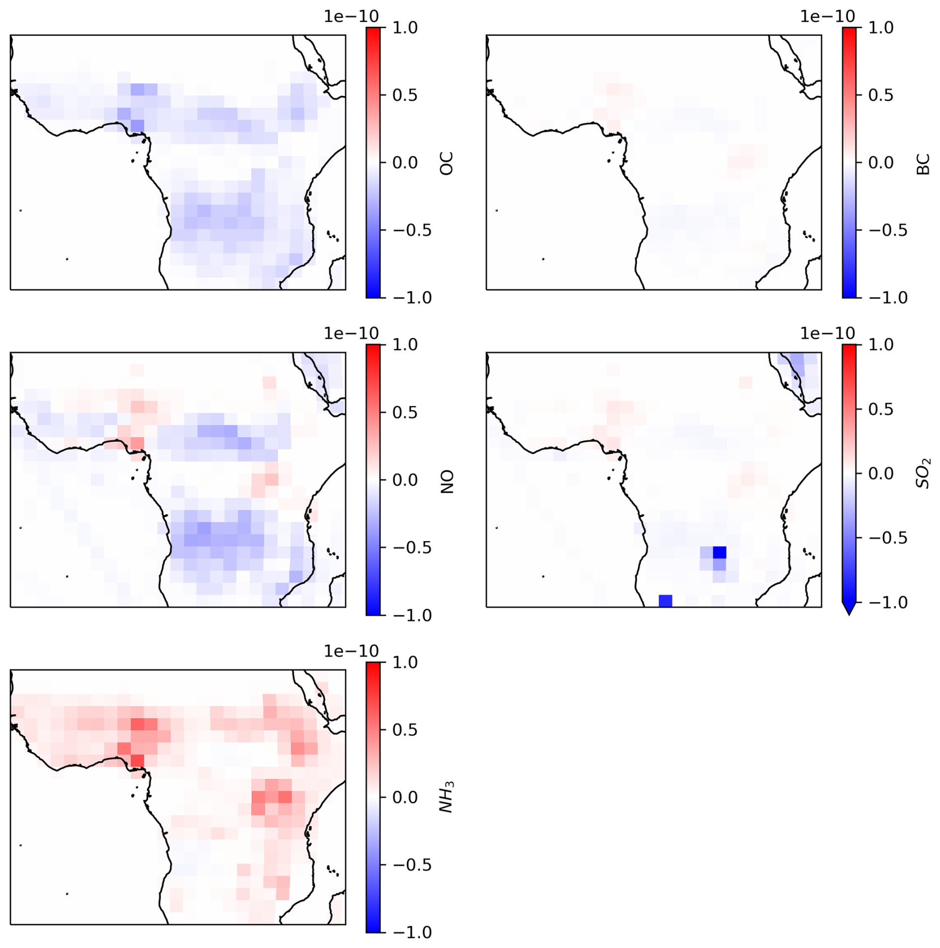
Figure 21 Changes in air pollutant emissions (kg m⁻² s⁻¹) in 2090 relative to 2020 over equatorial Africa under SSP3-7.0-lowNTCF.

To explore the potential sources of error and bias of GW-GPR emulator, we conduct more detailed analysis of ΔPM_2.5 over equatorial Africa in 2090 under SSP3-7.0-lowNTCF. Figure 21 shows the changes in OC, BC, NO, SO₂ and NH₃ emissions over equatorial Africa. Over Nigeria, the magnitudes of NO (+145 %), SO₂ (+180 %) and NH₃ (+140 %) emission changes are well beyond the range prescribed in our training set (±100 %), which could lead to failure of the machine learning algorithms. We also recognize GW-GPR has consistent positive biases over GCHP-CAM (Fig. 10) over equatorial Africa that cannot be effectively eliminated by switching to MLR (Fig. 12). This hints that the mismatch between regional pollutant transport patterns and the prescribed geographic weighting scheme could be another possible source of error of GW-GPR over equatorial Africa. Theoretically, the isotropic geographic weighting scheme only emulates of primary pollutants and precursors of secondary pollutants as a purely diffusive process, but not directly emulating the dispersion of secondary pollutants nor the advective components of pollutant dispersion. This might also contribute to the failure of the emulator to predict the changes in regional aerosol background, especially when the emission changes are highly spatially heterogenous.

The comparison between GW-GPR and AerChemMIP output shows that the GW-GPR emulator can generate predictions of ΔPM_2.5 that are within the range of output from mainstream chemistry-climate models at global scale, while requiring much less computational resources (at the order of 10–100 CPU seconds per scenario) to run. This confirms the utility of GW-GPR in predicting the spatiotemporal changes in anthropogenic PM_2.5 exposure under global change scenarios. However, GW-GPR predictions must be interpreted cautiously when the changes in emissions are well beyond that prescribed in the training set (±100 %), or there is large spatial heterogeneity in pollutant emission changes within a region.

5 Discussion

In this work, we apply a classic emulator building workflow (carefully sampling the input space to create samples for training machine learning models) that has been widely applied in engineering (Alizadeh et al., 2020) to build a reduced-form global model of anthropogenic PM_2.5 from a global 3D chemical transport model, GCHP-CAM. Similar techniques (also often choosing Gaussian Process Regression as the machine learning algorithm) have been used for uncertainty analysis and parameter calibration in atmospheric chemistry modelling (Reyes-Villegas et al., 2023; Ryan and Wild, 2021; Wild et al., 2020), and directly emulate air quality models at local and regional scales (Conibear et al., 2021; Vander Hoorn et al., 2022). Our work extends this approach for global change scenarios, where climate change, inter-regional chemical transport and different chemical regimes pose another layer of challenges.

To address these challenges, there are a few unique features of the emulator architecture in comparison to other reduced-form global air quality models. We design the emulator to be usable for a wide range of integrated assessment modelling and policy evaluation, where new scenarios or greenhouse gas concentration and pollutant emissions are routinely generated, but complementary atmospheric simulations are not always available. Therefore, rather than directly using the meteorological fields as input (e.g. Chen et al., 2023), we parameterize anthropogenic climate change intensity as a function of atmospheric CO₂ concentration, and use geographic weighting of pollutant emissions (Pisoni et al., 2018) to approximate the effect of chemical transport. Rather than exploring the source-receptor relationships between pre-defined regions, the emulator is trained at individual grid cell scale. Therefore, the accuracy of the emulator is not affected by different definitions of regions and sub-regional changes in spatial patterns pollutant emissions, which is important for application across different integrated assessment frameworks. This also allow us to tackle the non-linearity in the atmospheric chemical system by exploring more combinations of pollutant emission changes (more efficiently via Latin Hypercube Sampling) and machine learning (via Gaussian Process Regression).

By analysing emulator performance at grid cell scale, we find the GW-GPR emulator successful in reproducing the global and regional changes in PM_2.5 simulated by GCHP-CAM under 4 climate and air quality legislation (IGSM-GAINS-TAPS) scenarios. To evaluate the utility of the emulator, we show that it provides results within the range of full-scale models in the AerChemMIP archive under SSP3-7.0 and SSP3-7.0-lowNTCF scenarios. This shows our emulator can provide reasonable predictions under climate scenarios (in this case, SSP3-7.0) other than that used to train the emulator (i.e. the 10 W m⁻² scenario from IGSM), with the caveat that the magnitudes of climate change (and therefore climate impact on PM_2.5) could be misrepresented under overshoot scenarios, large decoupling between emission trajectories of CO₂ and other important GHGs (e.g. high CH₄ scenarios), and a significant difference in climate response with that simulated by IGSM-CAM (see Sect. 2.3.1). We also find that the emulator may underperform when (1) the magnitude of pollutant emission changes is well beyond that prescribed in the training set (±100 %); (2) the geographic weighting scheme ignores the advective component of pollutant transport, therefore misrepresents region-specific directional pollutant transport patterns; (3) the spatial pattern of pollutant emission changes is highly heterogenous within a region. This points to some potential ways of improving the accuracy of the GW-GPR framework (e.g. fitting anisotropic geographic weighting schemes for each grid cells, expanding the training set), which can be explored in the future.

In addition to the mean, GPR also calculates the standard deviation of the prediction, which can be interpreted to characterize the statistical uncertainty of emulator output. As unforced climate variability directly contributes to the interannual variabilities of PM_2.5, previous studies recommend 10–20 years of averaging to robustly detect the changes in PM_2.5 over the contiguous United States (Brown-Steiner et al., 2018; Garcia-Menendez et al., 2017; Pienkosz et al., 2019), especially when the signal to be detected is smaller or comparable in magnitude to the underlying unforced climate variability. Due to limitations in computing time, we focus on exploring a wider range pollutant emission and climate change by generating each sample in the training set using 1 year of simulation, rather than running multiple years of simulation to generating robust signals amidst unforced climate variabilities for each set of perturbation experiment. This significant source of uncertainty, however, is captured by the uncertainty quantification algorithm of the GPR. Therefore, in addition to the magnitude, our emulator also provides the uncertainties in ΔPM_2.5, which can be important in quantifying the overall uncertainties of health impacts of future air pollution (Saari et al., 2019).

In combination with the emission intensity projections from GAINS, TAPS can translate integrated assessment model output to spatially explicit air pollutant emission inventories. Combining with the GW-GPR emulator (Fig. 2), we can potentially produce grid cell scale projection of anthropogenic PM_2.5 changes for any climate and air quality integrated assessment scenarios within seconds, as demonstrated by our IGSM-GAINS-TAPS emulation exercise. This opens up the possibility for including air quality impacts within climate and sustainability decision making and scientific analysis. As climate projections move towards including scenario design as part of the uncertainty (Guivarch et al., 2022; Lamontagne et al., 2018; O'Neill et al., 2016, 2020), climate and global change scenarios generated will increase by orders of magnitude (Lamontagne et al., 2018; Shindell and Smith, 2019), where the runtime required by reduced-order chemical transport models (a few hundred CPU hours per model year) could be a hurdle for large ensemble modelling, despite their advantage of having higher spatiotemporal resolution than global statistical emulators; and statistical emulators that require meteorological fields as input would not be applicable as 3D climate simulations are too computationally expensive to be conducted for individual scenario. Tools with proper balance between accuracy, computing resource and input data requirements become more important in enabling uncertainty analysis, impact assessment human-Earth system feedback research. Our work shows the potential of machine learning techniques in enabling rapid and accurate global air quality assessment. Future work includes applying the PM_2.5 emulator to study more global change scenarios, representing other important climate-sensitive emission sources (e.g. wetland methane, dust, fire), improving and extending the emulator to calculate changes in other pollutants (e.g. O₃) and local climate forcing, and building a software package and web interface to increase the accessibility of the emulator.