swLICOM: the multi-core version of an ocean general circulation model on the new generation Sunway supercomputer and its kilometer-scale application

The global ocean general circulation model (OGCM) with kilometer-scale resolution is of great significance for understanding the climate effects of mesoscale and submesoscale eddies. To address the computational and storage demands of exponential growth associated with kilometer-scale resolution simulation for global OGCMs, we develop an enhanced and deeply optimized OGCM, namely swLICOM, on the new generation Sunway supercomputer. We design a novel split I/O scheme that effectively partitions tripole grid data across processes for reading and writing, resolving the IO bottleneck encountered in kilometer-scale resolution simulation. We also develop a new domain decomposition strategy that removes land points effectively to enhance the simulation capability. In addition, we upgrade the code translation tool swCUDA to convert the LICOM3 CUDA kernels to Sunway kernels efficiently. By further optimization using mixed precision, we achieve a peak performance of 453 Simulated Days per Day (SDPD) with 59 % parallel efficiencies at 1 km resolution, scaling up to 25 million cores. The result of simulation with a 2 km horizontal resolution shows swLICOM is capable of capturing the vigorous mesoscale eddies and active submesoscale phenomena.

1 Introduction

Improving the horizontal resolution of global ocean general circulation models (OGCMs) to the kilometer scale has been a cutting-edge direction in current physical oceanography research. The core goal is to resolve the nonlinear interactions of oceanic multi-scale dynamical processes. Though traditional high-resolution models with ∼ 10 km horizontal resolution can capture mesoscale eddy activities (Hallberg, 2013; Kjellsson and Zanna, 2017; Hewitt et al., 2020), they fail to directly resolve submesoscale processes with horizontal scales of 100 m–10 km (Gula et al., 2022; Xie et al., 2024), which contribute to key mechanisms such as energy cascade, vertical mixing, and material transport (Zhang et al., 2023; Chassignet and Xu, 2017; Schubert et al., 2019; Balwada et al., 2018; Soufflet et al., 2016). In recent years, with the breakthrough of supercomputing technology, global OGCMs with kilometer-scale resolution have been gradually realized. For example, the $\mathrm{1}/\mathrm{48}$° MITgcm LLC4320 simulation (Su et al., 2018), the ocean component of ICON-Sapphire with a 1.25 km resolution (Hohenegger et al., 2023), and the $\mathrm{1}/\mathrm{100}$° global model LICOMK++ (Wei et al., 2024; Xie et al., 2025). Such OGCMs show great capability on simulating submesoscale eddies and the related multi-scale interactions. However, limited by computing resources and storage costs, long-term integration (such as on the interannual scale) of kilometer-scale global OGCMs still faces challenges.

The rapid development of the heterogeneous supercomputers provides potential opportunities to solve the problem. The development of new climate and ocean models on heterogeneous supercomputers has advanced rapidly, demonstrating significant performance (Eirund et al., 2025; Silvestri et al., 2024), particularly in the GPU or DCU architectures. Fuhrer et al. (2018) rewrote the dynamical framework of the COSMO model, which implements solutions to the non-hydrostatic Euler equations, from Fortran to C++ (Fuhrer et al., 2018; Thaler et al., 2019). They developed the Stencil Loop Language (STELLA), a domain-specific programming C++ templates-based language (Gysi et al., 2015). STELLA provides performance-portable optimizations for stencil computations and can track data access patterns and kernel data dependencies. Although STELLA simplifies code porting, COSMO conversion still requires a significant amount of hand-written code. POM.gpu (Xu et al., 2015), a GPU version of mpiPOM, converts Fortran code to CUDA C and enhances its performance through loop and function fusion, better use of read-only data cache and L1 cache, multi-GPUs communication optimization, and overlapping I/O and computation. Kinaco which is a non-hydrostatic ocean model that was developed for high-resolution numerical ocean studies, focused on improving the sparse matrix-vector multiplication of its MGCG solver on GPUs, primarily optimizing data access and employing instruction-level parallelism and mixed precision computing (Yamagishi and Matsumura, 2016; Matsumura and Hasumi, 2008). For the porting of Veros to GPUs, Python with JAX backend was used (Häfner et al., 2021). PETSc and petsc4py were used to support distributed linear solvers. Veros provided a hand-written implementation of the Thomas algorithm, written in Cython for CPUs and CUDA for GPUs, to enhance efficiency. Oceananigans is the first ocean model designed specifically for GPUs rather than being ported from existing CPU code (Silvestri et al., 2023). Oceananigans utilized Oceananig-ans.jl, a new software written in the Julia programming language. It leverages Just-In-Time (JIT) compilation and LLVM to implement optimizations, including kernel fusion, on-the-fly computation for intermediate quantities, and overlapping computation and communication. In addition, there have been efforts to optimize POP on accelerators like Intel Xeon Phi. Key techniques include explicit and implicit fusion of data locality and vectorization, along with asynchronous offloading strategies for scheduling computations asynchronously (Aketh et al., 2016).

On the other hand, as another important heterogeneous supercomputer, significant model development of kilometer-scale resolutions has been achieved on Sunway architecture processors. Xu et al. (2019) developed SWSLL, a domain-specific language for stencil computations optimization of WRF's dynamical framework. SWSLL automates loop fusion and dependency analysis and partitions computations based on memory access counts, guided by the Roofline model, indicating memory-bound computations for stencils. CESM (Community Earth System Model) is ported to Sunway by manual kernel coding for the dynamical framework and OpenACC for physical process optimization (Zhang et al., 2020b). Ye et al. (2022) developed swNEMO, which implements simulation with a resolution of 1 km, achieving a performance of 1.43 SYPD.

In this study, we redesign and develop the LASG/IAP Climate system Ocean Model version 3.0 (LICOM3; Li et al., 2020; Lin et al., 2020) on the new generation Sunway supercomputer. LICOM3 was developed by the State Key Laboratory of Numerical Modeling for Atmospheric Sciences and Geophysical Fluid Dynamics (LASG), Institute of Atmospheric Physics (IAP), Chinese Academy of Sciences. The development of LICOM for heterogeneous supercomputers is evidenced by three key versions: LICOM2-gpu (Jiang et al., 2019), LICOM3-HIP (Wang et al., 2021), and LICOM3-CUDA (Wei et al., 2023), each specifically ported to a different computing architecture.

LICOM2-GPU utilized OpenACC to port LICOM2 to GPUs, employing techniques such as local memory blocking, loop fusion, and communication optimization. LICOM3-HIP utilized AMD's HIP interface for AMD GPU portability, facilitating code conversion and execution on both NVIDIA and AMD GPUs. LICOM3-CUDA, a CUDA C version of LICOM3, enhanced fine-grained parallelism, decoupled data dependencies, and prevented memory write conflicts, particularly optimizing heterogeneous architecture communication. LICOM3-CUDA outperforms LICOM3-HIP, making it the preferred choice for LICOM3 porting to the Sunway platform. The latest achievement is from our previous work named LICOMK++, a performance-portable OGCM that uses Kokkos. It achieves 1.05 SYPD performance for 1 km resolution on the new generation Sunway supercomputer (Wei et al., 2024). In this study, we explore new automatic code transformation methods beyond Kokkos and achieve better performance metrics than Kokkos for LICOM3 at the kilometer-scale resolution, contributing to ocean model development.

To support the kilometer-scale resolution simulation of LICOM3 and leverage the performance advantages of heterogeneous computing, we redesign and optimize LICOM3 on the new-generation Sunway supercomputer, naming the optimized model swLICOM. Section 2 introduces the new-generation Sunway supercomputer and the LICOM3 model. Our innovative methods and optimizations are detailed in Sect. 3. In Sect. 4, we evaluate the performance and scalability of swLICOM and present the ultra-high-resolution simulation results.

2 Model Description and HPC

2.1 The Ocean General Circulation Model

LICOM3 is a global OGCM to simulate the oceanic physical state and general circulation. It also serves as the ocean component of coupled climate models, such as the Flexible Global Ocean Atmosphere-Land System model (FGOALS; Bao et al., 2013; Li et al., 2013) and the Chinese Academy of Sciences Earth System Model (CAS-ESM; Zhang et al., 2020a). In addition, LICOM3 has participated in the Ocean Model Intercomparison Project Phases 1 and 2 (OMIP1 and OMIP2, respectively; Lin et al., 2020; Tsujino et al., 2020).

LICOM3 adopts the Arakawa-B grid horizontally and eta coordinates vertically (Mesinger et al., 1988) with free sea surface height. It utilizes orthogonal curvilinear coordinates and the tripolar grid (Smith et al., 1992, 2010). Its dynamical core also employs a two-step shape-preserving advection scheme and a semi-implicit mode-splitting (barotropic-baroclinic) time-stepping scheme.

If the coordinate system $({\mathit{\xi }}_{\mathrm{1}},{\mathit{\xi }}_{\mathrm{2}},{\mathit{\xi }}_{\mathrm{3}})$ is an orthogonal curvilinear coordinate system on a spherical surface and we only consider the changes in the horizontal grid coordinates on the sphere's surface while keeping the vertical coordinate system unchanged, the model primitive equations in any orthogonal curvilinear coordinate system are given by:

$$\begin{array}{}\text{(1)}& \left\{\begin{array}{l}\frac{\partial u_x}{\partial t}+L\left(u_x\right)=-\frac{\mathrm{1}}{{\mathit{\rho }}_{\mathrm{0}}{h}_{\mathrm{1}}}\frac{\partial p}{\partial {\mathit{\xi }}_{\mathrm{1}}}-f^{*}{u}_y+F_{mx}+\frac{\partial }{\partial {\mathit{\xi }}_{\mathrm{3}}}\left(K_m\frac{\partial u_x}{\partial {\mathit{\xi }}_{\mathrm{3}}}\right),\\ \frac{\partial u_y}{\partial t}+L\left(u_y\right)=-\frac{\mathrm{1}}{{\mathit{\rho }}_{\mathrm{0}}{h}_{\mathrm{2}}}\frac{\partial p}{\partial {\mathit{\xi }}_{\mathrm{2}}}+f^{*}{u}_x+F_{my}+\frac{\partial }{\partial {\mathit{\xi }}_{\mathrm{3}}}\left(K_m\frac{\partial u_y}{\partial {\mathit{\xi }}_{\mathrm{3}}}\right),\\ \frac{\partial p}{\partial z}=-\mathit{\rho }g,\\ \frac{\mathrm{1}}{h_{\mathrm{1}}{h}_{\mathrm{2}}}\left(\frac{\partial h_{\mathrm{2}}{u}_x}{\partial {\mathit{\xi }}_{\mathrm{1}}}+\frac{\partial h_{\mathrm{1}}{u}_y}{\partial {\mathit{\xi }}_{\mathrm{2}}}\right)+\frac{\partial w}{\partial {\mathit{\xi }}_{\mathrm{3}}}=\mathrm{0},\\ \frac{\partial T}{\partial t}+L\left(T\right)=A_T{\mathrm{\nabla }}^{\mathrm{2}}T+\frac{\partial }{\partial {\mathit{\xi }}_{\mathrm{3}}}\left(K_T\frac{\partial T}{\partial {\mathit{\xi }}_{\mathrm{3}}}\right)+C_T+Q_{\mathrm{pen}},\\ \frac{\partial S}{\partial t}+L\left(S\right)=A_S{\mathrm{\nabla }}^{\mathrm{2}}S+\frac{\partial }{\partial {\mathit{\xi }}_{\mathrm{3}}}\left(K_S\frac{\partial T}{\partial {\mathit{\xi }}_{\mathrm{3}}}\right)+C_S,\\ \mathit{\rho }=\mathit{\rho }(T,S,p),\end{array}\right.\end{array}$$

where T and S are temperature and salinity respectively, ρ is the in-situ density, p is the pressure, f^* is the Coriolis parameter, Q_pen is the shortwave radiation penetration term, K_m is the vertical turbulent viscosity coefficient for velocity, K_T and K_S are the vertical turbulent diffusion coefficients for temperature and salinity respectively, A_T and A_S are the horizontal turbulent diffusion coefficients for temperature and salinity respectively, C_T and C_S are the vertical advection terms, F_mx and F_my are the horizontal turbulent viscosity terms, ∇² is the horizontal Laplacian operator, L is the advection operator, u_x and u_y are the horizontal velocities in the directions of the orthogonal curvilinear basis vectors along the spherical surface, where h_i is known as the Lamé coefficient. The physical meaning of the Lamé coefficients is the length of the unit basis vectors in an orthogonal curvilinear coordinate system when projected onto a Cartesian coordinate system, which represents the true length in physical space. Therefore, the Lamé coefficients are also known as map scale factors. The horizontal viscosity terms in the momentum equations can be written as (Griffies, 2009):

$$\begin{array}{}\text{(2)}& {\displaystyle }\begin{array}{rl}{F}_{mx}& =A_m({\mathrm{\nabla }}^{\mathrm{2}}{u}_x-u_x\left({\displaystyle \frac{\partial K_x}{h_{\mathrm{1}}\partial {\mathit{\xi }}_{\mathrm{1}}}}+{\displaystyle \frac{\partial K_y}{h_{\mathrm{2}}\partial {\mathit{\xi }}_{\mathrm{2}}}}+\mathrm{2}{K}_x^{\mathrm{2}}+\mathrm{2}{K}_y^{\mathrm{2}}\right)\\ & +u_y\left({\displaystyle \frac{\partial K_x}{h_{\mathrm{2}}\partial {\mathit{\xi }}_{\mathrm{2}}}}-{\displaystyle \frac{\partial K_y}{h_{\mathrm{1}}\partial {\mathit{\xi }}_{\mathrm{1}}}}\right)+\mathrm{2}{K}_y\left({\displaystyle \frac{\partial u_y}{h_{\mathrm{1}}\partial {\mathit{\xi }}_{\mathrm{1}}}}\right)\\ & -\mathrm{2}{K}_x\left({\displaystyle \frac{\partial u_y}{h_{\mathrm{2}}\partial {\mathit{\xi }}_{\mathrm{2}}}}\right)),\end{array}\text{(3)}& {\displaystyle }\begin{array}{rl}{F}_{my}& =A_m({\mathrm{\nabla }}^{\mathrm{2}}{u}_y-u_y\left({\displaystyle \frac{\partial K_x}{h_{\mathrm{1}}\partial {\mathit{\xi }}_{\mathrm{1}}}}+{\displaystyle \frac{\partial K_y}{h_{\mathrm{2}}\partial {\mathit{\xi }}_{\mathrm{2}}}}+\mathrm{2}{K}_x^{\mathrm{2}}+\mathrm{2}{K}_y^{\mathrm{2}}\right)\\ & +u_x\left({\displaystyle \frac{\partial K_y}{h_{\mathrm{1}}\partial {\mathit{\xi }}_{\mathrm{1}}}}-{\displaystyle \frac{\partial K_x}{h_{\mathrm{2}}\partial {\mathit{\xi }}_{\mathrm{2}}}}\right)+\mathrm{2}{K}_x\left({\displaystyle \frac{\partial u_x}{h_{\mathrm{2}}\partial {\mathit{\xi }}_{\mathrm{2}}}}\right)\\ & -\mathrm{2}{K}_y\left({\displaystyle \frac{\partial u_x}{h_{\mathrm{1}}\partial {\mathit{\xi }}_{\mathrm{1}}}}\right)),\end{array}\end{array}$$

where A_m is the horizontal turbulent viscosity coefficient, $K_x\equiv \frac{\mathrm{1}}{h_{\mathrm{1}}{h}_{\mathrm{2}}}\frac{\partial h_{\mathrm{2}}}{\partial {\mathit{\xi }}_{\mathrm{1}}}$, $K_y\equiv \frac{\mathrm{1}}{h_{\mathrm{1}}{h}_{\mathrm{2}}}\frac{\partial h_{\mathrm{1}}}{\partial {\mathit{\xi }}_{\mathrm{2}}}$.

Except for the Laplace term in Eqs. (2) and (3), all other terms are geometric curvature terms, which arise due to the non-uniformity of the coordinate grid in physical space. Additionally, under any orthogonal curvilinear coordinates, the expressions for the advection operator and the two-dimensional Laplacian operator are as follows:

$$\begin{array}{}\text{(4)}& \left\{\begin{array}{l}L=u_x\frac{\partial }{h_{\mathrm{1}}\partial {\mathit{\xi }}_{\mathrm{1}}}+u_y\frac{\partial }{h_{\mathrm{2}}\partial {\mathit{\xi }}_{\mathrm{2}}}+w\frac{\partial }{\partial {\mathit{\xi }}_{\mathrm{3}}},\\ {\mathrm{\nabla }}^{\mathrm{2}}=\frac{\mathrm{1}}{h_{\mathrm{1}}{h}_{\mathrm{2}}}\left(\frac{\partial }{\partial {\mathit{\xi }}_{\mathrm{1}}}\left(h_{\mathrm{2}}\frac{\partial }{h_{\mathrm{1}}\partial {\mathit{\xi }}_{\mathrm{1}}}\right)+\frac{\partial }{\partial {\mathit{\xi }}_{\mathrm{2}}}\left(h_{\mathrm{1}}\frac{\partial }{h_{\mathrm{2}}\partial {\mathit{\xi }}_{\mathrm{2}}}\right)\right).\end{array}\right.\end{array}$$

Equations (1) to (4) represent a system of differential equations in arbitrary orthogonal curvilinear coordinates (Yu et al., 2018b).

LICOM3 essentially solves the equations described above. The main procedure for solving these equations is illustrated in Fig. 1. Seven compute-intensive modules operate within the time integration loop: “readyt”, “readyc”, “barotr”, “bclinc”, “tracer”, “icesnow”, and “convadj”. These modules are the primary targets for optimization. The first two modules compute terms in the barotropic and baroclinic equations. The following three modules (“barotr”, “bclinc”, and “tracer”) are responsible for solving the barotropic, baroclinic, and temperature/salinity equations. The prescribed data are used for ice module. The “icesnow” module has been simplified to only handle temperatures higher or lower than the freezing point of the seawater, usually using −1.8 °C in the model. The “convadj” module is the convective adjustment, which ensures that the density of the lower layer of seawater is greater than that of the upper layer.

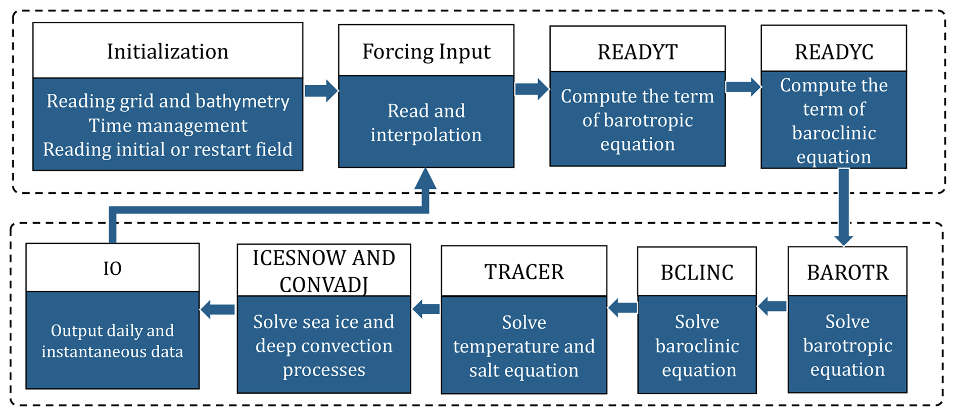
Figure 1 The overview of LICOM3 architecture. The INITIALIZATION module is responsible for model initial preparation, including reading grid and bathymetry file, reading initial or restart field, and time management. The main procedure includes seven main compute-intensive modules and IO module: READYT for computing terms of the barotropic equation, READYC for computing terms of the baroclinic equation, BAROTR for solving the barotropic equations, BCLINC for solving the baroclinic equations, TRACER for solving the tracer (temperature and salinity) equations, ICESNOW and CONVADJ for solving sea ice and deep convection process, IO module for outputting daily and instantaneous data.

2.2 SW26010 Pro

SW26010 Pro is a new generation of Sunway heterogeneous many-core processors developed by China. It builds upon the basic architecture of the SW26010 and serves as an improved version of the processor featured in the Sunway TaihuLight supercomputer.

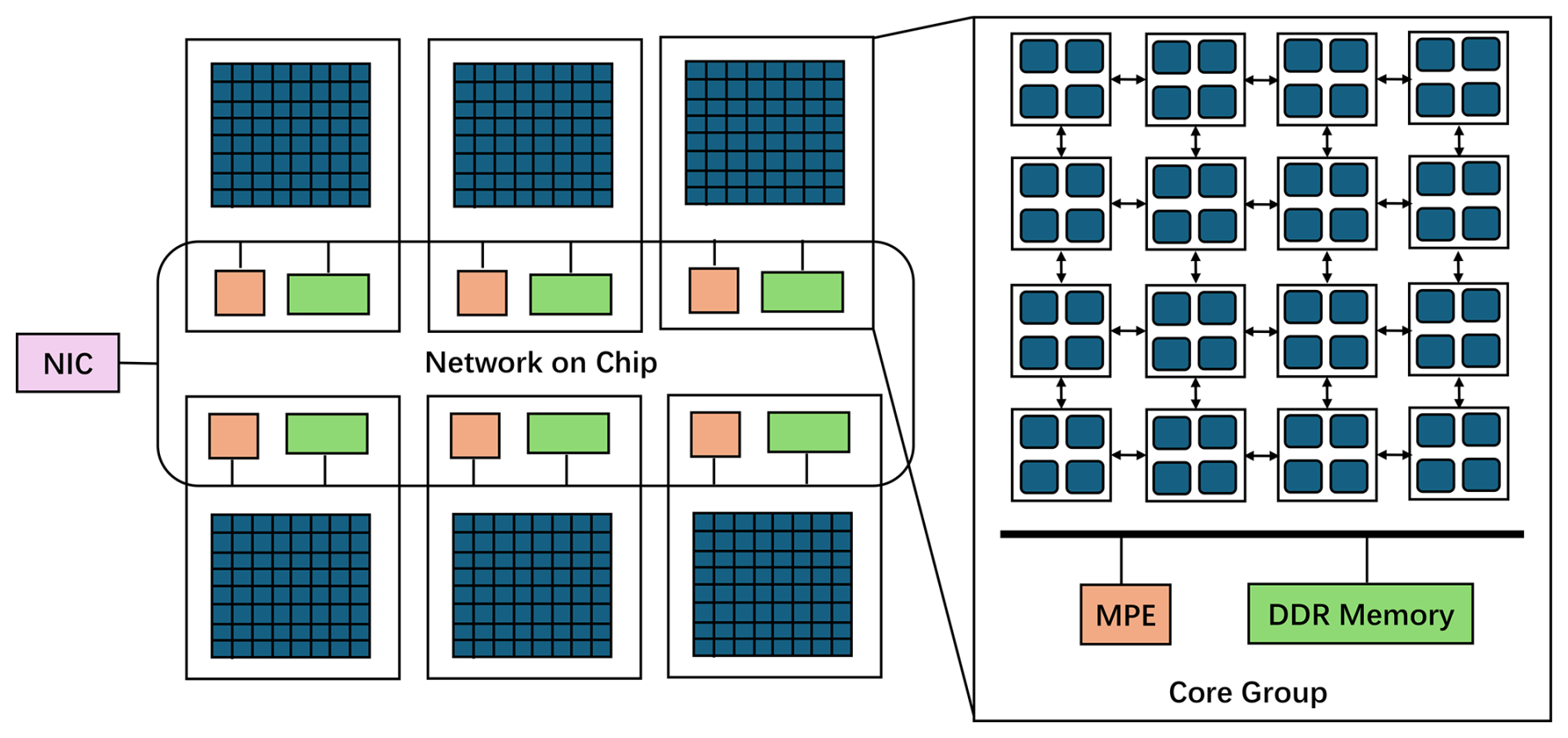
Figure 2 The architecture of SW26010 Pro many-core processor. Each SW26010 Pro processor contains 6 Core Groups (CGs). Within each CG, there are one management processing element (MPE) and 64 computing processing elements (CPEs) organized in an 8×8 cluster and 16 GB of attached DDR4 main memory. These 6 CGs and network interface card (NIC) are connected via the network on chip (NoC).

The architecture of SW26010 Pro is shown in Fig. 2. The SW26010 Pro is divided into six core clusters, known as Core Groups (CGs). Each CG consists of one Management Processing Element (MPE) and 64 Computing Processing Elements (CPEs). MPE is responsible for handling communication, IO, and spawning threads on CPEs. CPEs in each CG are organized as an 8×8 mesh and communicate with each other using Remote Memory Access (RMA). The MPE features a 32KB L1 Instruction cache, 32KB L1 Data Cache, and 512KB L2 cache. Each CPE has a 32KB L1 Instruction cache and a 256 KB software-managed scratchpad called local data memory (LDM) with up to half configurable as cache. Each CG has its own memory controller and a 16 GB memory capacity, providing the SW26010 Pro chip access to a total of 96 GB of main memory. Each CG has its own memory controller and has 16 GB of memory capacity. In total, a SW26010 Pro chip can access 96 GB of main memory. CPEs can access main memory through Load/Store instructions or direct memory access (DMA). These 6 CGs and network interface cards (NICs) are connected via the network on-chip (NoC). Each node contains a single chip with its own network connectivity. A Supernode connects 256 nodes via a high-speed switch. Each Supernode is further connected to a cross-supercomputer interconnect with 48 ports. The heterogeneity of arises from two distinct core types within each chip, the general-purpose MPEs and lightweight CPEs with separate memory hierarchies and instruction sets. (Lin et al., 2023). Compared to traditional multi-core architectures, the heterogeneous many-core architecture poses more complex programming challenges, necessitating significant efforts to redesign and optimize applications to harness its full computational potential. The new generation Sunway supercomputer is equipped with more than 100 000 SW26010-Pro chips, each with 390 cores, and is one of the fastest supercomputers globally.

The Athread programming model is a parallel programming model for the Sunway architecture. It provides an abstraction that is closely mapped to the Sunway hardware. It offers explicit control mechanisms for managing the DMA controller on the CPEs. This allows programmers to efficiently move data between the main memory (controlled by the MPE) and the LDM of each CPE, which is crucial for overcoming memory bandwidth bottlenecks. The typical execution flow involves the main program running on an MPE. The MPE calls “athread_spawn” interface to create “slave” threads that execute a specified function on the CPEs. All threads in the team execute the same function, but on different portions of the data. The Athread programming model provides synchronization primitives (e.g., barriers) to coordinate the execution of these threads. The MPE calls “athread_spawn” to wait for the code execution to finish.

The primary challenge in optimizing for the SW26010 Pro processor stems from its heterogeneous architecture. In this architecture, the MPE handles inter-process communication and controls the overall application workflow. The main computing power, however, resides in the CPEs. Each CPE is equipped with a manually managed LDM that offers access speeds comparable to the L1 cache. CPEs can communicate directly via Remote Memory Access (RMA). To leverage the CPEs' computational capacity, code executed initially on the MPE must be ported to an Athread kernel. The MPE is responsible for launching this kernel and subsequently waiting for its completion. Consequently, effectively leveraging the unique characteristics of the CPEs is the key to achieving high performance.

3 Method and Optimzations

3.1 swCUDA

LICOM3 was ported to different supercomputer clusters in recent years (Wang et al., 2021). Every time, porting LICOM3 and getting superior performance takes a huge effort. In the GPU version of LICOM3, there are a total of more than 70 kernels that are manually ported and optimized. To address this issue, we adopt an auto-parallel code translation tool, swCUDA, to automatically translate the mature CUDA kernel of LICOM GPU version to Sunway Athread kernel from our previous work (Yu et al., 2024). swCUDA constructs a hardware mapping model and a scaled affine algorithm between GPU and Sunway CPE. Meanwhile, a set of high-level directives is designed, which is easy to implement. For general usage, only the attribute and pattern of data need to be specified. Considering the characteristics of LICOM3 kernels with general stencil computation, We optimized the swCUDA to version 1.1, automatically achieving 3D grid decomposition and memory optimization. This upgrade gives translated kernels better parallel scalability. swCUDA 1.1 supports various memory transfers to accomplish auto-translation based on the high-level directive. The architecture of swCUDA 1.1 is shown in Fig. 3. Firstly, high-level directives are embedded to illustrate the attributes and patterns of the data in the CUDA kernel, as shown in Fig. 3b. Secondly, the code generator ANTLR (Parr et al., 2014) is utilized to parse the CUDA kernel to an abstract syntax tree (AST). Thirdly, our translation algorithms are utilized in corresponding AST nodes to accomplish CUDA primitive translation and memory redirection. By swCUDA 1.1, the Sunway kernel is translated not only with high efficiency but also with high performance.

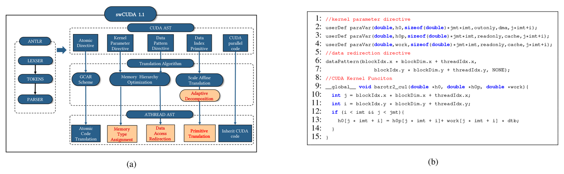
Figure 3 swCUDA 1.1 overview. swCUDA 1.1 automatically translates the CUDA kernel to the Athread kernel by using high-level directives. (a) The workflow of swCUDA 1.1. swCUDA adopts a hardware mapping model and scaled affine algorithm between GPU and SW26010 Pro. ANTLR is used to parse CUDA kernels to CUDA AST. Our algorithm translates the CUDA AST to the Athread AST and generates the ATHEAD kernel. We promote adaptive decomposition and memory accessing optimization in swCUDA 1.1. (b) An example of swCUDA 1.1 usage. Kernel parameter directive userDef paraVar and data redirection directive dataPattern are specified to implement memory accessing optimization in translation.

3.1.1 Adaptive Decomposition

LICOM3 uses finite-difference approximation to solve the Navier–Stokes equations, the general stencil computation in a multidimensional grid. In the LICOM model, space is discretized into 3-D grid points. Horizontal grid points are labeled as (i, j). Each grid point represents multiple levels, which correspond to various vertical heights in the ocean; the vertical height is denoted as k. Most data structures (arrays) in LICOM are three-dimensional arrays with the layout of (i, j, k). The elements in Fortran's arrays are stored in column-major order. Therefore, elements in dimension i are stored continuously in memory. Because there are different computational patterns in LICOM, different decomposition schemes are used for different patterns. For example, “jk decomposition” means that the computation is decomposed by assigning tasks with different j and k ranges to different CPEs. In the GPU version of Licom3, the grid is decomposed into two or three-dimensional thread blocks. Each thread block has fixed threads depending on the hardware limit, which is divided as a cube, as shown in Fig. 4a. However, this decomposition is not adapted to the Sunway platform since it conducts data swapping in the cache to increase the cache miss rate. Hence, we designed an integrated “jk decomposition” to improve Sunway parallel efficiency, as shown in Fig. 4b. By this decomposition, the whole grid is divided into multiple i-directional blocks. With data stride, blocks with the same color are sent to the same CPE. Data access in each CPE is continuous, which is the most effective cache utilization.

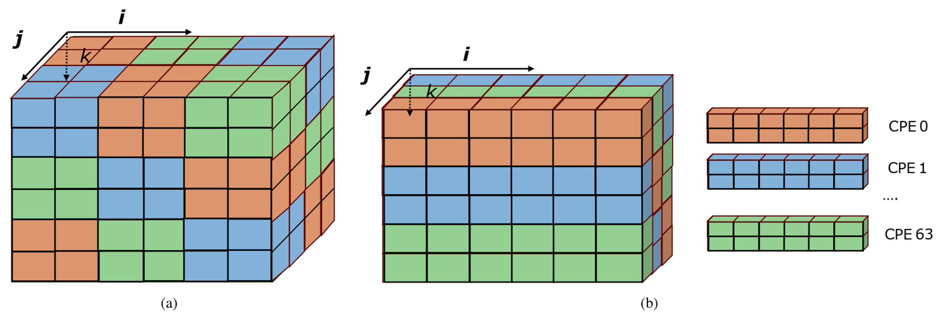
Figure 4 The decomposition translation between CUDA on NVIDIA GPU and Athread on Sunway processor. (a) Three dimensions of a 3D block decomposition for the CUDA kernel. (b) An integrated “jk decomposition” of a 3D block data decomposition for the Athread kernel.

To automatically translate GPU decomposition to Sunway-integrated “jk decomposition”, we develop an adaptive decomposition method in swCUDA. In the original CUDA thread hierarchy, there is a limit to the number of threads per block, which may contain up to 1024 threads. Here, we break through this limit by directly assigning i-dimensional data to thread blocks as one-dimensional blocks and decomposing the grid into j and k-dimensional blocks, automatically according to different parallel scales. Each CPE is assigned with continuous blocks for load balance. Each block occupies continuous i-directional data for access and calculation. Based on this translation, the original CUDA parallel algorithm can be inherited in Sunway kernels and achieves the most optimal performance.

3.1.2 Memory Accessing Optimization

In the previous swCUDA, we designed a general memory optimization strategy. It provides a flexible memory type interface, which is automatically distributed according to the variable memory size. However, the variable memory size of LICOM3 is changed in different parallel scales. Meanwhile, many stencil kernel computations require access to data from its surrounding grids with three dimensions in LICOM3, which means discrete memory access is a general characteristic. In Sunway CPE, slave L1 cache direct access is suitable for continuous data access, and discrete memory access should be leveraged by DMA transfer. Selecting appropriate memory usage is essential to promote kernel performance. Hence, we redesign our high-level directive to explicitly illustrate the data memory usage and localization of data indexing for specific data arrays by the format paraVarAttr(type,varname,size,inout,memUsage,glbInx), as shown in Fig. 3b. Each data array has a detailed attribute. The inout attribute indicates whether the array is read-only or modified within the kernel. memUsage is used to describe if it uses cache or DMA transfer. glbInx is required to combine with dataPattern for usage, which represents the global thread indexing pattern for i, j, and k directions in the CUDA kernel. glbInx denotes the global indexing pattern of the current array. If the array uses DMA transfer, swCUDA translates the global indexing to local indexing using our new jk decomposition algorithm. Otherwise, swCUDA directly translates its index to global indexing. Based on this new strategy, most kernels perform better due to the appropriate memory usage.

3.1.3 Manually Optimization

In CUDA kernels, stencil computation is not concerned with the order of the three-dimensional loop since all data has been loaded into the GPU device memory. However, Sunway kernels are very sensitive to the k-loop position. If the k loop is in the innermost layer, the efficiency of the Sunway kernel is worse; even the method of using DMA transfer can't address this issue. In this case, we need to manually optimize the kernels. There are two ways. One is to extract the k loop to the outer based on trading space for time. Another method is to decompose data by ik decomposition, as shown in Fig. 5. From our example in Fig. 5a, WKK is extended to a three-dimensional data array wktmp to record data in every grid point, which can extract k-loop to outer. Then, the Sunway kernel can use jk decomposition with continuous data access. As shown in Fi. 5b, data is decomposed from the i- and k-directions. Each CPE is assigned part of the i-directional and total k-directional data using stride DMA transfer. Data is reorganized and loaded to Sunway CPE with the continuous array. Hence, data indexing is required for redirection. The manual optimizations are used in several kernels to improve the performance significantly.

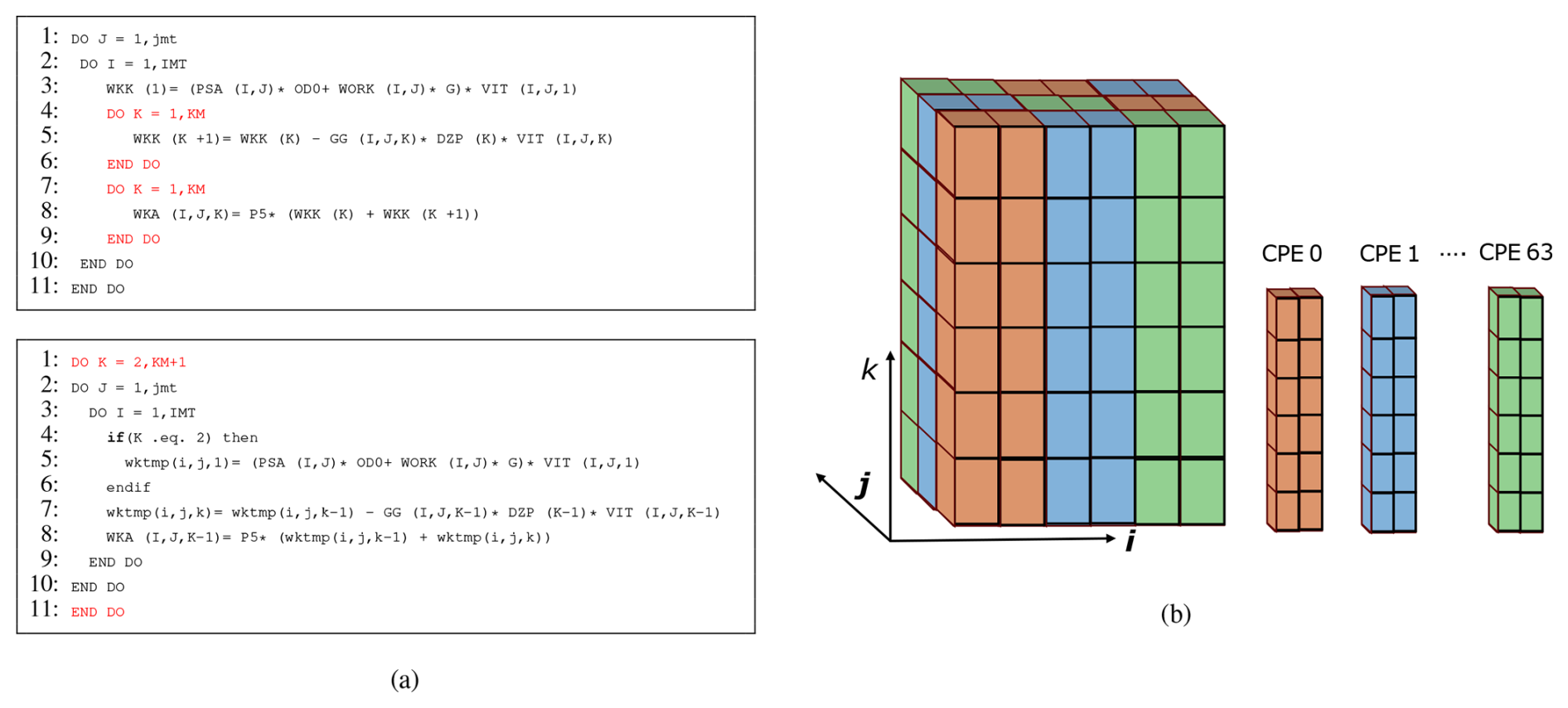
Figure 5 Manual optimization is needed to change the loop order from jik to kji. (a) An example of extracting the k loop to the outer. The upper code snippet is the original stencil computation with k in the inner loop, and the lower one is the optimized code, extracting the k loop to the outer based on trading space for time. (b) An example of the IJ directional decomposition. Part of the i and j directional data is assigned and loaded to each CPE.

3.2 Remove Land Grid Points

To accelerate computations and reduce resource usage, we optimize the LICOM grid partition. The total land area globally accounts for 29 % of the Earth's total surface area. When partitioning the Earth's surface into grids, the number of grid points on the land represents approximately 29 % of all grid points. However, land points have no effect on marine points and do not contribute to the final results. Therefore, we design an algorithm to remove land grid points to reduce resource usage and improve computing efficiency, as shown in Fig. 6. First, the input data is partitioned according to the number of processes. Each process holds one block of data, and each block holds tens of grid points. Then, we count the marine grid points of each block. If no marine grid points exist in one block, we will remove the process corresponding to the block. A pre-processing procedure is implemented to tackle the problem. During the actual computation, we will launch the processes containing marine points. For accurate calculations, we need to map the process rank that only includes marine points to the original process rank that did not exclude land points. In this way, we can correctly read and write the data. At the same time, we will regenerate a new communication topology based on the new process rank to facilitate the exchange of boundary data. Through this approach, we can reduce 29 % in computational resources while ensuring that the results are completely consistent with the original results, thus increasing computational speed and resource efficiency at high resolution.

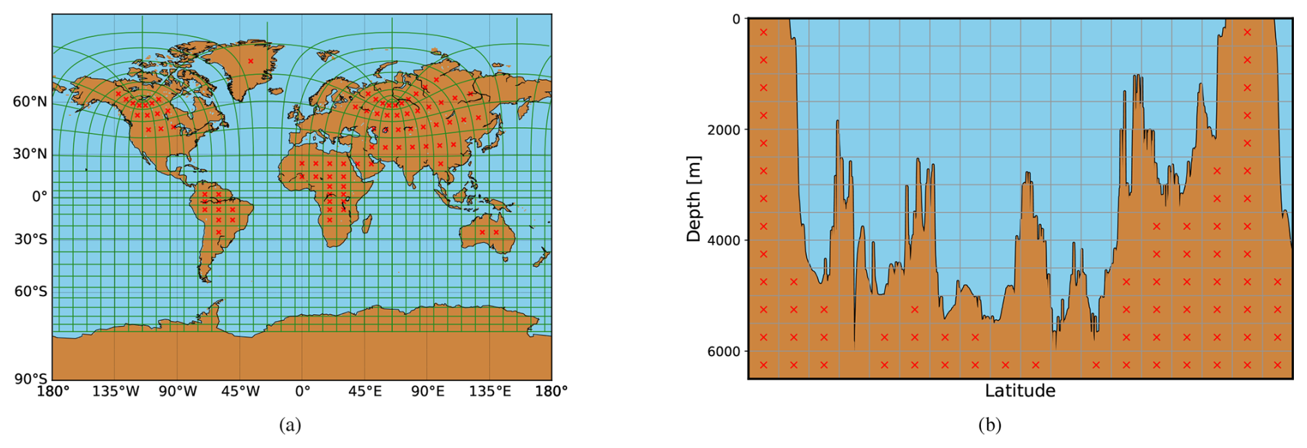
Figure 6 Manual optimization for removing land grid points. (a) Removing land-only MPI processes. The MPI process decomposition of the LICOM3 tripole grid (green lines). Each block contains many grid points for both ocean and land, and the blocks are labeled by a red ×, indicating that the block contains only land grids. (b) Removing land points in the vertical dimension. The grid points in one block are ocean or land in the vertical dimension. The land points in one block are labeled by a red ×.

3.3 IO Optimizations

LICOM utilizes the NetCDF format to read input, write model output, and restart files. Initially, data are read by a single process, which then distributes them among others. Similarly, output data from multiple processes is gathered by one process and written to the file system. However, as the number of processes increased to hundreds of thousands, input reading and output writing performance became inadequate. To address this issue, we adopted a strategy that divides the data into multiple subfiles, as shown in Fig. 7. To minimize the number of subfiles, each set of one hundred processes handles input reading from a single subfile, and similarly, one hundred processes collectively write model output and restart files to a single file. Furthermore, we opted for a binary format for both input and output files. Compared to the original NetCDF-based implementation, this optimized approach has significantly improved IO performance across tens of thousands of compute nodes.

For analysis and archival storage purposes, a post-processing step involves several nodes that convert the binary format data into the NetCDF format.

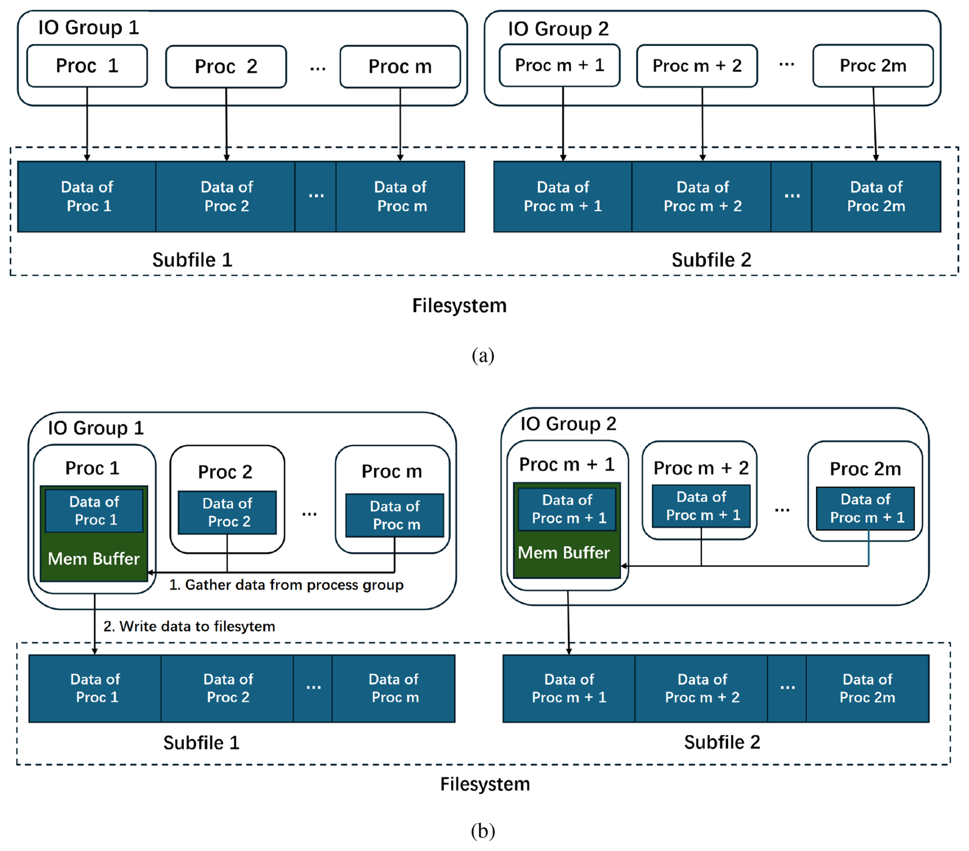
Figure 7 IO strategy. The big files have been separated into small subfiles. All MPI processes are divided into IO process groups that read from or write to a subfile. (a) Read data. Processes read their data based on their address offset in the subfile. (b) Write data. The master process in the lO process group first gathers data from other processes. Then, the master process writes data to a subfile.

3.4 Mixed Precision

The ocean model default uses double resolution to guarantee the simulation accuracy, regardless of the need. The computational cost and memory bandwidth increase exponentially along with the in-depth application of kilometer resolution in the ocean model. The approach of reducing numerical precision has been proven to be an effective strategy to improve performance (Tintó Prims et al., 2019; Chen et al., 2024). We implement single precision mainly focusing on Eqs. (5) and (6) of LICOM3, making a balance of performance improvement and fidelity.

3.4.1 Selecting Variable of Reduced Precision

In swLICOM, we divide the set of variables into three groups: dynamic core, tracer formulation, and physical package. The dynamic core mainly consists of barotropic and baroclinic processes. The tracer primarily calculates temperature and salinity equations. The physical package mainly includes vertical viscosity and diffusivity schemes (Canuto et al., 2002a). Most of the variables in these three groups are relatively independent. For these three groups, the tracer formulation occupies almost 50 % of the computational cost (Wang et al., 2021). Canuto parametrization (Canuto et al., 2002b) which is the vertical viscosity and diffusivity schemes in LICOM only calculates vertical diffusivities for momentum, heat, and salt. Hence, our reduced precision is aimed at the variables of tracer formulation and physical package, which occupy more than 75 % amount of the total variables. Furthermore, Canuto parametrization is heavily computing-intensive and load-unbalanced. In this case, implementing reduced precision can significantly promote its performance. On the other hand, advection momentum calculation in dynamic core requires higher precision since its equation may encounter the circumstance of multiplying a small value by a big value, which causes a significant loss of precision or even a NAN value, as shown in shown in the Eqs. (5) and (6). Here, adv_uu and adv_vv represent the advection momentum component in the θ and λ direction. Hence, the tracer formulation and the Canuto parametrization are implemented in single precision in swLICOM.

$$\begin{array}{}\text{(5)}& {\displaystyle }\begin{array}{rl}\mathrm{adv}\mathrm{\_}{\mathrm{uu}}_{i,j,k}& =-{\left(u{\displaystyle \frac{\partial u}{\partial \mathit{\theta }}}\right)}_{i,j,k}-{\left(v{\displaystyle \frac{\partial u}{\partial \mathit{\lambda }}}\right)}_{i,j,k}\\ & -{\left({\displaystyle \frac{\partial wu}{\partial z}}\right)}_{i,j,k}\end{array}\text{(6)}& {\displaystyle }\begin{array}{rl}\mathrm{adv}\mathrm{\_}{\mathrm{vv}}_{i,j,k}& =-{\left(u{\displaystyle \frac{\partial v}{\partial \mathit{\theta }}}\right)}_{i,j,k}-{\left(v{\displaystyle \frac{\partial v}{\partial \mathit{\lambda }}}\right)}_{i,j,k}\\ & -{\left({\displaystyle \frac{\partial wv}{\partial z}}\right)}_{i,j,k}\end{array}\end{array}$$

3.4.2 Design Accuracy Test

The metric used to evaluate the similarity between double and mixed precision versions is root mean square deviation (RMSD) (Ye et al., 2022). However, directly using RMSD to evaluate the accuracy is not appropriate. LICOM is developed to a variable resolution gridpoint model by adopting tripolar grids (Yu et al., 2018a). Hence, the area of each grid point is different. Due to this reason, we need to utilize the area of each grid for our accuracy formula instead of the original number of gridpoints to get a more accurate deviation:

$$\begin{array}{}\text{(7)}& \mathrm{MIXRMSD}\left(t\right)=\sqrt{{\displaystyle \frac{\sum _{i=\mathrm{1}}^{i_{max}}\sum _{j=\mathrm{1}}^{j_{max}}\left(\right({\mathrm{dbl}}_{i,j}\left(t\right)-{\mathrm{mix}}_{i,j}\left(t\right){)}^{\mathrm{2}}{\mathrm{area}}_{i,j})}{\sum _{i=\mathrm{1}}^{i_{max}}\sum _{j=\mathrm{1}}^{j_{max}}{\mathrm{area}}_{i,j}}}}.\end{array}$$

In this formula, i,j are the spatial grid indice, t is the time index, dbl_i,j(t) is the value in double precision version at the given i,j gridpoint and given t time. mix_i,j(t) is the corresponding value in the mixed precision version. area_i,j is the area of each grid with a unit of square kilometer.

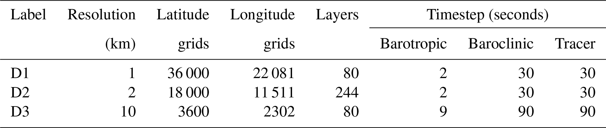
Table 1 Configuration of our grids and timesteps. The case of 10 km resolution is used to implement performance metrics to quantify the performance improvement of new domain decomposition. The case of 1 and 2 km resolution is used to evaluate the fidelity of swLICOM and the performance of swLICOM. The maximum grid point we adopted is beyond 63 billion.

4 Experiments and test results

4.1 Model Configuration

All of our evaluations are conducted in a new generation of Sunway HPC. Comprehensive experiments on a kilometer-scale are performed to evaluate the performance and fidelity of our new swLICOM with 1, 2, and 10 km resolution, respectively. The model configuration is shown in Table 1. To ensure a fair comparison in our scalability tests, we evaluated all data resolutions by employing the time step of the highest-resolution simulation as the universal time step. Therefore, only one factor, resolution, changes across all these experiments. Despite the different resolution, the region stays the same, from 76° S to 90° N. Forcing field is adopted by Japanese 55-year Reanalysis for driving ocean–sea-ice models (JRA55-do) with 3 h frequency (Tsujino et al., 2018), except runoff and sea-ice with daily frequency. We use the bilinear method to interpolate the forcing field to map with different model resolutions. The case of 10 km resolution is a classical case based on the previous LICOM experiment (Wang et al., 2021; Wei et al., 2023). It is used to break down our innovations to quantify the performance improvement of new domain decomposition, I/O optimization, and mixed precision, etc. The case of 1 and 2 km ultra-high resolution is used to evaluate the strong extensibility of swLICOM. Meanwhile, we use the case of 2 km resolution to evaluate the fidelity of swLICOM by hindcast simulation. The performance indicators are represented by using SDPD (simulated-days-per-day).

4.2 Performance Metric

To evaluate our innovations, a set of software versions is listed in Table 2. The version of LICOM-Org is the original version ported from the Intel platform, which is calculated by MPE cores. Each innovative method is separately implemented into different software versions for evaluation. To perform performance analysis and profiling accurately, we port the GPTL library (Version 8.1.1) into LICOM software and manually insert GPTL instrumentation. We use the max time interval of MPI ranks for statistics. The time consumption of both module computation and I/O processes can be accurately measured. We utilize 10 km resolution with time steps set to 9, 90, and 90 s for the barotropic, baroclinic, and tracer, respectively. We implement three different parallel scales for each comparison. The performance improvement is shown in Fig. 8.

Table 2 LICOM software version list. LICOM-Org is the original version as a benchmark. The others are optimized versions implementing our innovative method separately, which are used to verify performance improvement.

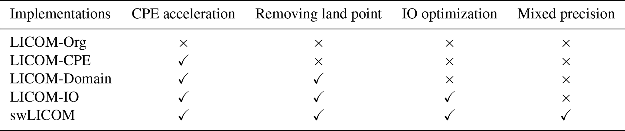
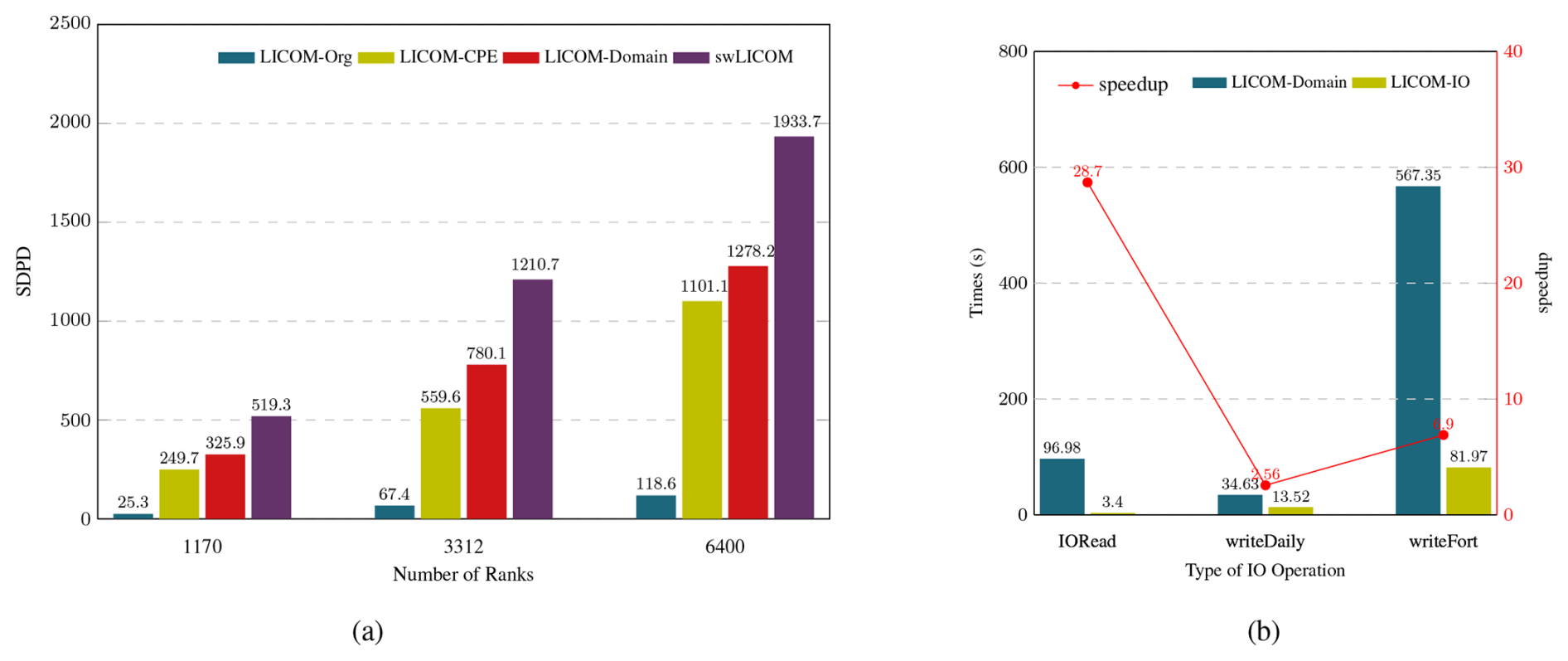
Figure 8 The performance improvement and IO optimizations. (a) The performance (Simulated Days per Day, SDPD) for the original version of LICOM (LICOM-Org, blue bar) as a reference and three main optimizing versions, including porting to CPE (LICOM-CPE, yellow bar), removing land points (LICOM-Domain, red bar), and the mix-precision (swLICOM, purple bar) on three scales run with 1170, 3312, and 6400 ranks. (b) The performance of the IO time in a single simulation day for LICOM-Domain (blue bar) as a reference and the IO-optimized version LICOM-IO (yellow bar) for the reading files (IORead), writing daily mean files and restart files (writeDaily), and writing instantaneous files (writeFort) on single scales with 1170 ranks. The red line is the speedup. The LICOM-Domain version here uses serial NetCDF reading and PNetCDF parallel writing.

As shown in Fig. 8a, our accelerated LICOM-CPE version gets a maximum 12.3 times speedup compared with the original LICOM version with 1170 ranks. Along with the parallel scale's growth, speedup times are decreased since more time is spent on MPI communication.

To fairly evaluate the performance of our new removing land point domain decomposition, we use three identical parallel scales for verification. We adopt original Cartesian domain decomposition for LICOM-CPE and new Cartesian_noland decomposition for LICOM-Domain version. From the different parallel scales, we can get an average above 30 % speedup. This significant improvement is because there is no need to implement meaningless calculations on land points and boundary data exchange with land points. Especially in a large parallel scale, the new domain decomposition will save more than 10 million cores.

Mixed precision is implemented in our final swLICOM version. We get an average of 1.5 times speedup compared with the double precision version LICOM-IO. The main contribution is that the parametrization scheme of Canuto in LICOM is totally implemented with a single precision. It decreases the load balance among ranks, which indirectly causes less time spent in the following halo update in the barotropic process.

Our breakdown experiment demonstrates that each innovation method has significantly improved performance. Ultimately, we get a maximum speedup of 20 times for swLICOM compared with the LICOM-Org version.

IO experiment is implemented to simulate 1 d on 1170 ranks, which is configured as startup mode, writing history file every 6 h and a daily file per day, as shown in Fig. 8b. The IORead is the total time of reading the initial field, forcing field, and grid data. The writeDaily and writeFort represent the time of writing instantaneous files and daily files, respectively. The speedup of IORead is up to 28.7. The reason is that in the original version, data is read by a single core and then scattered to the whole ranks, according to tripole boundary conditions. If this original reading method is used in the 1 km/2 km experiment with super high parallel scales, the time spent will exponentially increase. By using our split reading strategy, the time spent will be kept the same at 10km resolution. Although PNetCDF (Parallel I/O Library for NetCDF File Access) is used in the original LICOM version for writing, our new split writing scheme still shows its advantages with 2.56 and 6.9 times speedup than PNetCDF.

4.3 Performance and Results

The weak scalability test is evaluated by our final version swLICOM. We choose six different resolutions with the exact latitude and longitude block per rank and the same barotropic and baroclinic steps, as shown in Table 3. The horizontal resolutions range from 10 to 1 km, with cores increasing from 284 310 to 25 326 145. As shown in Fig. 9, we achieve 92 % parallel efficiency under the maximum 25 326 145 cores. The linear tendency chart along different resolutions demonstrates good weak scalability of swLICOM.

Table 3 Weak Scaling Configuration and timesteps. We select six different resolutions, ranging from 10 to 1 km, to implement a weak scalability test. Each resolution is adopted with the same latitude and longitude block per rank and the same barotropic and baroclinic steps.

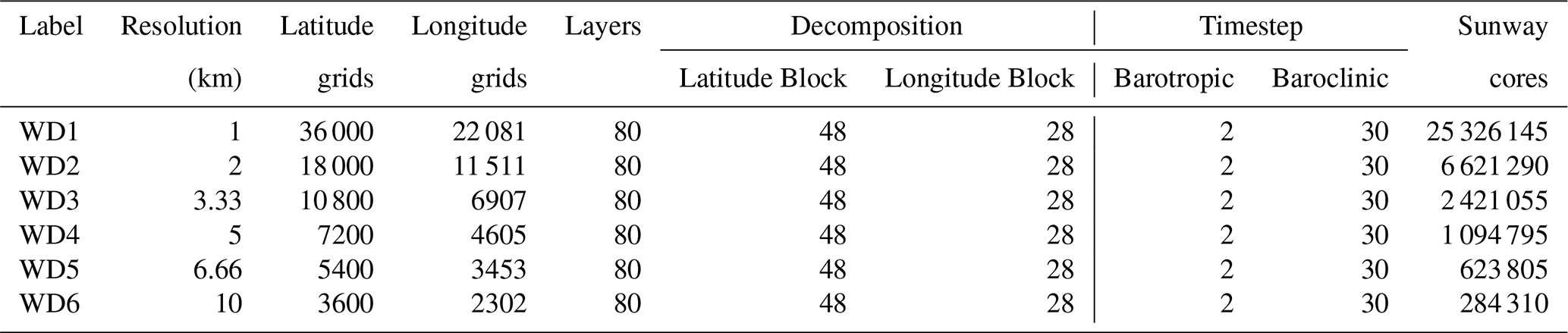
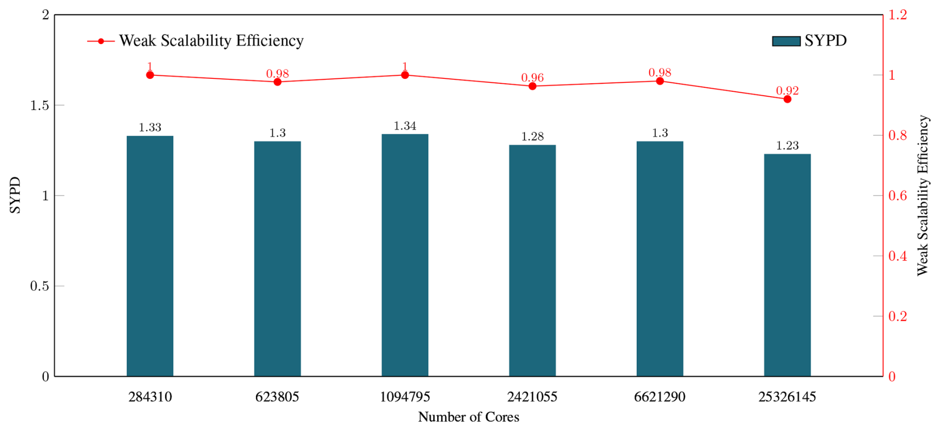
Figure 9 The weak scaling for swLICOM (Simulated Years per Day, SYPD) with 6 different resolutions of 1, 2, 3.33, 5, 6.66, and 10 km and the scaling of 284 310, 623 805, 1 094 795, 2 421 055, 6 621 290 and 25 326 145 cores, respectively. The red line is the efficiency.

We conduct a strong scalability test with 1 and 2 km resolution, respectively, which is configured as D1/D2, shown in Table 1. The 2 km test starts from 1 277 770 cores to 24 315 850 cores, and the 1 km test starts from 1 201 070 to 26 995 020. The strong scaling test result is shown in Fig. 10. We achieve peak performance of 410 SDPD with 45 % parallel efficiency at 2 km resolution and 453 SDPD with 59 % parallel efficiency at 1 km resolution. Although the total grid points of 1 km resolution are 1.25 times more than 2 km resolution, the parallel efficiency and SDPD of 1 km resolution are obviously better than 2 km resolution. The main reason is that the more vertical layers conduct the more memory access, and lower the performance.

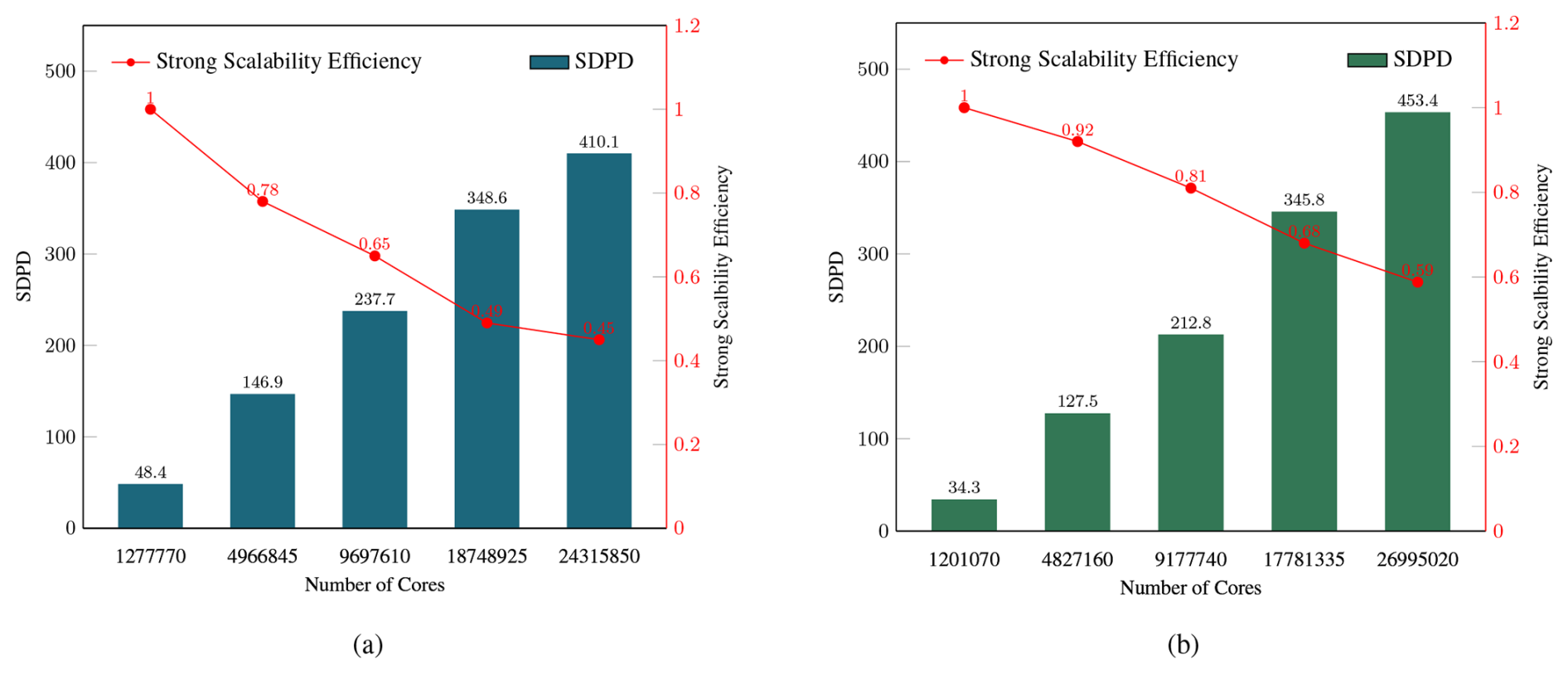
Figure 10 The strong scaling of swLICOM (Simulated Days per Day, SDPD) for (a) Strong scalability of 2 km resolution. 2 km test ranging from 1 277 770 to 24 315 850 cores and (b) Strong scalability of 1 km resolution. 1 km test ranging from 1 201 070 to 26 995 020 cores. The red lines are the efficiency.

To verify the accuracy of mixed precision, we conducted a one-month simulation on both the double precision version of LICOM-Domain and the mixed precision version of silicon. As introduced in Sect. 3.4.2, we calculate the average value of 30 daily data points for temperature, salt, and sea surface height. Then, we use our accuracy formula MIXRMSD to evaluate the accuracy, as shown in Fig. 11. The MIXRMSD of temperature, salt, and sea surface height is around 0.018, 0.0098, and 0.0005, respectively.

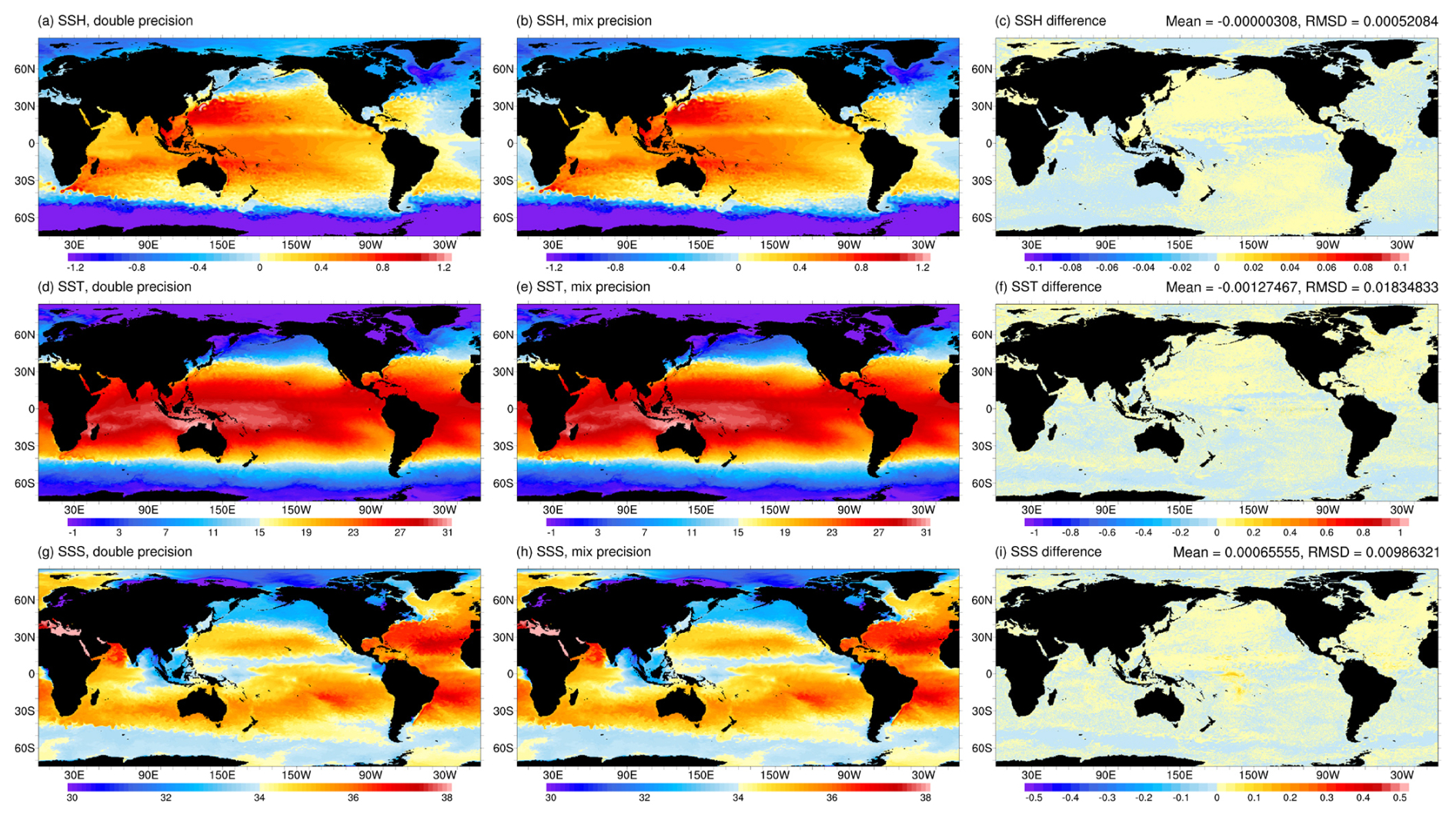
Figure 11 The monthly mean sea surface height (unit: m) for (a) double precision, (b) mixed precision, and (c) their difference in January 2016, simulated by swLICOM at a 10 km resolution. Panels (d)–(f) are for sea surface temperature (unit: °C) and (g)–(i) are for sea surface salinity (unit: psu). The upper right side shows the global mean and root-mean-square difference of the corresponding variables.

We use swLICOM with a horizontal resolution of 2 km to conduct a short-term (50 d) simulation test in the new generation Sunway cluster. Figures 12 and 13 show the snapshots of sea surface variables in the Kuroshio and Gulf Stream regions, respectively. The normalized vertical vorticity field, defined as $(\frac{\partial v}{\partial x}-\frac{\partial u}{\partial y})/f$, demonstrates active submesoscale processes with the magnitude of O(1), especially along the energetic jets and around the mesoscale eddies. The sea surface temperature field can also show clues of stirring submesoscale activities.

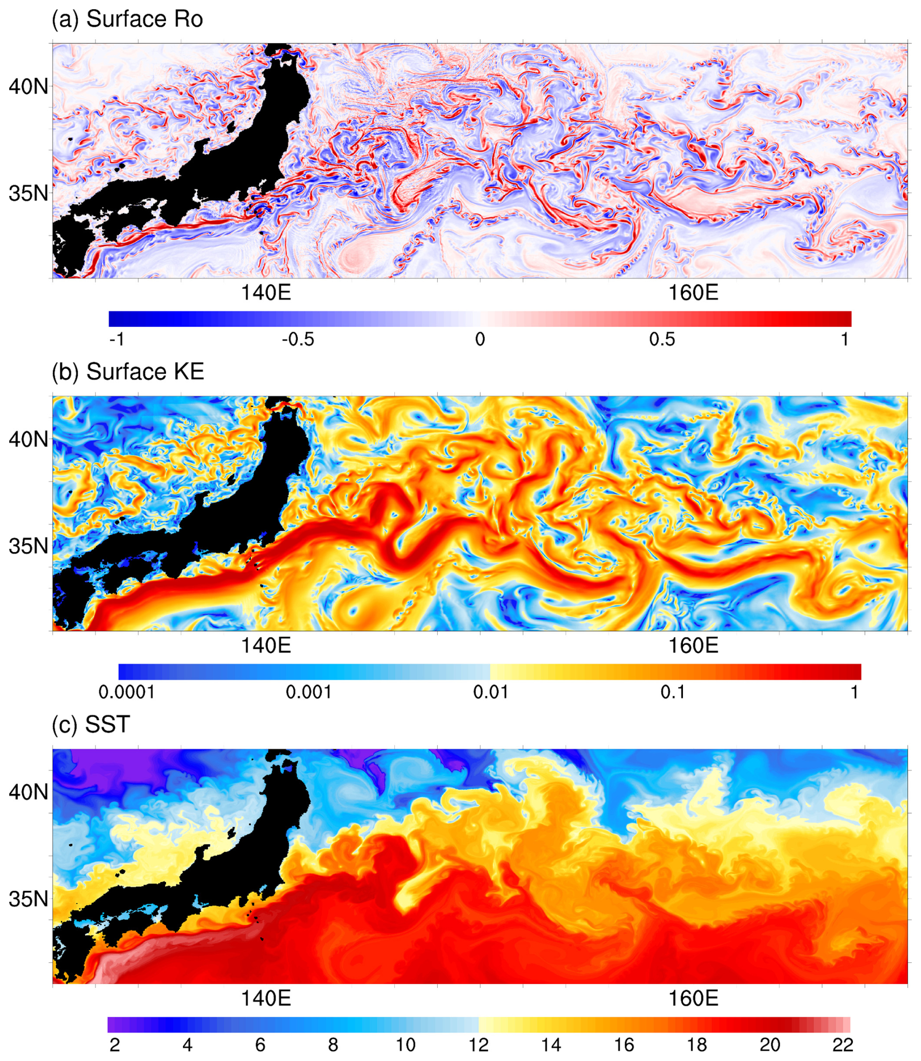
Figure 12 Snapshots of (a) surface normalized vertical vorticity (unit: 1), (b) surface kinetic energy (unit: m² s⁻²), and (c) sea surface temperature (unit: °C) in the Kuroshio region on 20 February 2016 simulated by swLICOM with a 2 km horizontal resolution.

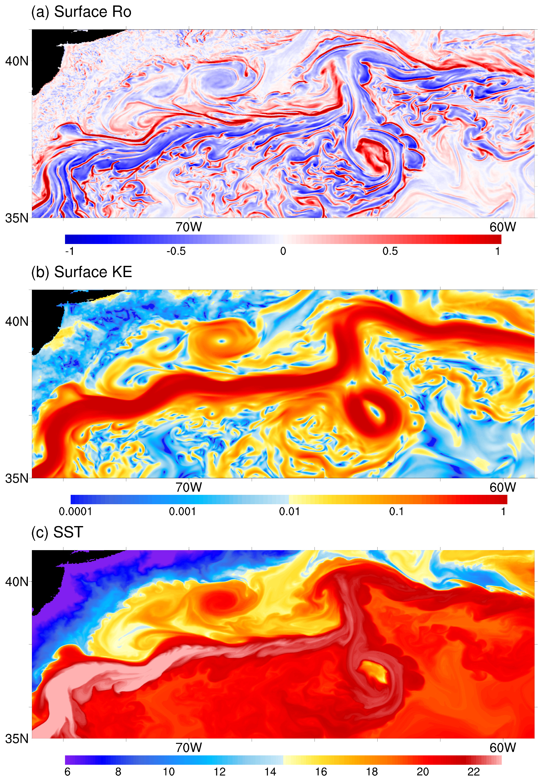
Figure 13 Same as Fig. 12, but for the Gulf Stream.

5 Conclusions

In conclusion, swLICOM represents a significant advancement in kilometer-scale resolution ocean general circulation models on heterogeneous computing architectures. By optimizing LICOM3 for the new generation Sunway supercomputer, we successfully address several key challenges associated with ultra-high-resolution global simulations. Through our effort, swLICOM demonstrates a peak performance of 453 SDPD with 59 % efficiencies at a 1 km resolution on 26 995 020 cores and 410 SDPD with 45 % efficiencies at a 2 km resolution on 24 315 850 cores in terms of strong scalability. Moreover, swLICOM captures the vigorous mesoscale eddies and active submesoscale phenomena with 2 km horizontal resolution.

Our optimization efforts addressed a series of challenges that are particularly crucial for high-resolution modeling. The automatic parallel code translation tool, swCUDA, is optimized to enhance computational performance and simplify the porting process for future applications, thereby promoting productivity and scalability. The initialization phase suffers from scalability limitations due to extreme parallelism processes and point-to-point (send-recv) communication patterns. Meanwhile, output operations require gathering hundreds of gigabytes of data into a single process, creating severe bottlenecks in write performance. To tackle the problem, a split I/O scheme is developed to improve IO bandwidth for large-scale computation and simulation capability at kilometer-scale resolutions. The time for both initialization and output operations are reduced from several hours to approximately 10 min for ultra-high-resolution simulations. Moreover, removing land points from computations significantly reduces the computational resources required for high-resolution simulation while maintaining the integrity of marine-related computations. This method can achieve an average about 30 % speedup which corresponds to the proportion of land area relative to Earth's total surface area. Furthermore, mixed precision is implemented to reduce memory usage and improve communication bottlenecks for such a large scale. The proposed implementation can gain about 50 % speedup versus the double-precision implementation. The adaptive decomposition method and memory access optimizations further contribute to the overall efficiency by maximizing cache utilization and improving data transmission speed. The adoption of bilinear interpolation or a forcing field significantly improves simulation accuracy.

Implementing swLICOM on the Sunway supercomputer sets a benchmark for future OGCM developments, highlighting the potential of heterogeneous computing in advancing climate and oceanographic studies. We use swLICOM with a horizontal resolution of 2 km to conduct a short-term (50 d) simulation test. The 2 km resolution global simulation shows the high capacity of swLICOM to capture the oceanic meso- to submesoscale processes.