DSCALE v0.1 – an open-source algorithm for downscaling regional and global mitigation pathways to the country level

Integrated Assessment Models (IAMs) provide low-carbon scenarios at a global scale or for broad economic aggregates, as running these models for every country would be computationally demanding. Lack of national results from IAMs, hinders the enhancement of NDCs (Nationally Determined Contributions) and LTS (Long Term Strategies) in accordance with the 1.5 °C target and best available science. To address this limitation, we have developed DSCALE (Downscaling Scenarios to the Country level for Assessment of Low carbon Emissions), a novel algorithm designed to downscale regional IAMs outcomes to the country level. In this paper we present the methodology and show results for both current policy and 1.5 °C scenarios from the NGFS 2023 release. This downscaling tool provides insights for energy and emission developments and targets at the country level consistent with global scenarios from IAMs. Moreover, this tool facilitates the integration of IAMs results with other models and tools requiring energy and emissions data at the country level, such as the macroeconomic NiGEM model.

1 Introduction

The Paris Agreement aims at holding temperature increase to well below 2 °C and pursue efforts to limit temperature to 1.5 °C. In this context, countries have submitted their NDCs (Nationally Determined Contributions) and LTS (Long Term Strategies) to the UNFCCC (United Nations Framework Convention on Climate Change) to mitigate emissions. However, collective efforts stated in the NDCs are not in line with the long term goal of the Paris Agreement (Dafnomilis et al., 2024; den Elzen et al., 2022; Fransen et al., 2023; Geiges et al., 2020; Hausfather and Moore, 2022; Iyer et al., 2022; Meinshausen et al., 2022; Emissions Gap Report 2023, 2024), as temperature is projected to increase to about 2–2.4 °C by the end of the century and with an estimated emissions gap of 19–27 GtCO₂ in 2030 (CAT, 2024). To fill this gap, new rounds of NDC revisions need to reflect highest possible ambition (UNFCCC, 2023), in keeping with the science (UNFCCC, 2015). In this context, Integrated Assessment Models (IAMs) can be used to provide useful insights on how to decarbonize global economies in line with the Paris Agreement, while minimizing mitigation costs. In 2018 the IPCC published a special report on 1.5 °C, with a focus on a global scale and large economic aggregates. The IPCC Sixth Assessment Report (AR6) reiterated the need for deep and immediate emissions reduction to keep global warming below 1.5 °C (IPCC, 2022). Applying insights from the IPCC, mostly based on IAMs (Battiston et al., 2021; Drouet et al., 2021; Riahi et al., 2021; van Soest et al., 2021) has remained difficult as most of these models focus on large economic aggregates. Modelling teams that develop and apply models including REMIND (Dietrich et al., 2023), WITCH (Emmerling et al., 2016) and MESSAGE (Huppmann et al., 2019; Ünlü et al., 2024) are tackling this issue by increasing the spatial heterogeneity. However, running these models for all countries in the world still comes with downsides regarding increased computational time and increased data requirements, particularly in regions with limited available data. This trade-off between resolution-uncertainty, computational time, and complexity has led many modelling teams to opt for grouping countries into regions.

Due to the limited regional resolution of Integrated Assessment Models (IAMs), monitoring progress towards the Paris Agreement has primarily focused on selected economies such as the G20 and other key countries (Baptista et al., 2022; den Elzen et al., 2022; Kuramochi et al., 2021; Nascimento et al., 2022; Peters et al., 2017; Roelfsema et al., 2020). Other studies encompassing a broader range of countries often employ equity principles to allocate greenhouse gas (GHG) emissions (Höhne et al., 2011; Meinshausen et al., 2015; Pont et al., 2016; Zimm and Nakicenovic, 2020). These allocations usually require deep emissions reductions in developed economies in the short term to offset historical emissions, often resulting in unrealistic reductions and excessive deployment of Carbon Dioxide Removals (CDR) in certain countries (Yang et al., 2023). Additionally, meeting the goals of the Paris Agreement entails the widespread deployment of renewables and low-carbon technologies, which are often overlooked in emissions pathways based on equity principles.

In the global stocktaking process, it is essential to identify gaps in current NDCs and LTS to align them with the long-term goal of the Paris Agreement and set up concrete actions for transitioning away from fossil fuels and foster deployment of renewables in a realistic manner. This process can be enhanced by utilizing downscaling techniques to adapt regional Integrated Assessment Model results (IAMs) to the country level. This study presents DSCALE (Downscaling Scenarios to the Country level for Assessment of Low carbon Emissions), a new algorithm designed to downscale Integrated Assessment Models (IAMs) results to the country level. We illustrate the methodology and demonstrate its application using scenarios from the NGFS (Network for Greening the Financial System) project (Richters et al., 2023). We downscale a current policy and 1.5 °C pathway from the MESSAGE model, with the aim to identify gaps and align country level trajectories and domestic goals with the objectives of the Paris Agreement. To this end, we provide results for 143 countries, including emissions as well as final, secondary, and primary energy variables.

This paper is structured as follows: the next section provides an overview of the main downscaling methods, a methodology section (and subsections covering different steps in the process) outlines the DCALE algorithm, a results section presents the downscaled country-level outcomes derived from the MESSAGE model for selected countries, a sensitivity analysis explores the feasibility range associated with various downscaling assumptions, a hindcasting section evaluates the performance of the tool when applied to historical data, and finally, a discussion section addresses the strengths and limitations of the approach and a conclusion section summarizes the findings.

Downscaling of scenarios

Downscaling methods have found applications in various domains, including modelling climate change impacts using Global Climate Models (GCMs) (Ekström et al., 2015; Hewitson et al., 2014), and analysing emissions pathways from Integrated Assessment Models (IAMs) (van Vuuren et al., 2007; Grübler et al., 2007; Fujimori et al., 2017a).

Downscaling approaches can be classified in terms of simple downscaling algorithms (Gaffin et al., 2004; Höhne and Ullrich, 2005), methods of intermediate complexity such as statistical models (Kheir et al., 2023; Khorrami et al., 2023), machine learning (Agarwal et al., 2023; Hobeichi et al., 2023; Jebeile et al., 2021; Li et al., 2019; Najafi et al., 2011; Niazkar et al., 2023; Sachindra et al., 2018; Vandal et al., 2019), and conditional modelling (Bollen, 2004; Carter et al., 2004; Sferra et al., 2019).

Different methods are chosen depending on the variables to be downscaled. Simple method such as linear downscaling (Höhne et al., 2011), use fixed shares to allocate regional data to the country level over the entire time horizon of future scenarios. A key advantage of this method is its simplicity, and it is usually employed for downscaling emissions, such as the SRES scenarios (van Vuuren et al., 2007). However, as the shares are calculated based on historical data from a given year, in the long term it could lead to overestimation of results in developed economies, compared to developing. To solve this problem, shares can be calculated dynamically over time based on proxy variables, from other models or scenarios. This method is referred as “external input-based” downscaling and it is generally used for downscaling socio-economic data (Gütschow et al., 2016, 2024; van Vuuren et al., 2007). However, this method could introduce systematic errors, as proxy variables could have been generated from scenarios with different underlying storylines or modelling assumptions, and therefore they may not be fully correlated with the variable of interest.

By contrast, statistical methods are usually employed for downscaling climate variables. These methods hinge on the assumption that the regional climate is affected by the large-scale climatic state and the local topography, including land use and land-sea distribution (von Storch, 1995). They offer calculations that are computationally inexpensive and therefore can be applied to many studies. However, a key limitation of these methods is the (unverifiable) assumption that historical relationship will hold true for future scenarios (Wilby et al., 2004). Machine learning approaches represent a further advancement, as they can efficiently unveil relationship among many climate variables. However, these methods require large amount of good quality data to adequately train the model. In addition, they raise issues about the interpretation of the results and transparency, as the rationale behind the results is hidden to the user (Carvalho et al., 2019).

Finally, conditional modelling requires coupling distinct models, usually making it more computationally intensive. For this reason, this method is often applied only for selected countries or variables. Achieving comprehensive downscaling with this method may require appropriate models for each country, potentially leading to extensive documentation and eventually lack of transparency.

Downscaling can be performed at the country level, at the subnational level such as cities, or at a grid level (spatial downscaling). Spatial downscaling is usually required for downscaling the forest land cover and land use or agriculture emissions (Chakir, 2009; Chen et al., 2020b; Hasegawa et al., 2017; Shi et al., 2021; Yourek et al., 2023). Apart from land use, studies focusing on sub-national downscaling usually rely on national (country-level) pathways as starting condition (Chen et al., 2020a; Viguié et al., 2014).

In the realm of country level downscaling, the literature often leans on algorithms based on IPAT/Kaya equations (Ehrlich and Holdren, 1971; Kaya, 1995; van Vuuren et al., 2007), primarily focusing on GHG emissions (Fujimori et al., 2017a; Gidden et al., 2018, 2019). These algorithms operate on the premise that GHG emissions are influenced by population size, affluence, and technology. According to the IPAT/Kaya approach, the impact on emissions is represented as the product of population, energy intensity (defined as final energy divided by GDP), and emissions intensity (defined as emissions divided by final energy). Usually country-level intensities converge to the regional level at a given time of convergence. However, a notable limitation of the standard IPAT/Kaya approach is that it does not explicitly account for the energy mix associated with carbon emissions.

In this study, we enhance the conventional IPAT/Kaya framework by calculating energy-related carbon using primary energy variables by fuel for each country (please refer to the model description section). The advantage of this new approach is the ability to explore the energy mix associated to low-carbon pathways, projected deployment of low-carbon technologies and negative emissions from BECCS (biomass with Carbon Capture and Storage), as well as land use emissions at the country level, on top of energy demand trajectories for end-use sectors such as industry, transportation, and buildings. Additionally, this tool incorporates country-level emissions targets such as the 2030 NDCs (Nationally Determined Contributions) goals and long-term (mid-century) strategies, thereby enhancing the realism of downscaled results. To the best of our knowledge, this is the first study to furnish a consistent array of downscaled data comprising emissions, final, secondary, and primary energy variables for 143 countries.

The DSCALE (Downscaling Scenarios to the Country level for Assessment of Low carbon Emissions) algorithm builds on previous work on downscaling energy variables based on the SIAMESE (Simplified Integrated Assessment Model with Energy System Emulator) approach (Sferra et al., 2019). Compared to SIAMESE, which provides a single emissions trajectory in each country, this new tool aims at providing a range of results to explore the scope of national targets consistent with IAMs scenarios in line with the Paris Agreement. National targets depend on boundaries conditions stemming from regional IAMs scenarios, as well as starting conditions at the country level. Hence, varying assumptions aimed at either maintaining disparities across countries or fostering greater convergence among them, result in a spectrum of pathways and associated targets.

Finally, a fundamental aspect of the downscaling of emission results involves understanding the characteristics of IAM scenarios, which are rooted in the socioeconomic framework of Shared Socioeconomic Pathways (SSPs) (Bauer et al., 2016, 2017; Fricko et al., 2017; Riahi et al., 2017a, b). This framework has been adopted by the research community on climate change to facilitate the integrated analysis of mitigation, adaptation and climate impacts (Moss et al., 2010; O'Neill et al., 2014, p. 214; van Vuuren et al., 2014). The SSPs provide narratives (O'Neill et al., 2014) and quantitative socio-economic projections of GDP (Dellink et al., 2017) and population (Samir and Lutz, 2017) at the country level, forming the basis for IAM scenarios. For example, scenarios from the Network for Greening the Financial System (NGFS) within the SSP2 (Middle of the Road) storyline (Fricko et al., 2017; Riahi et al., 2017a), present intermediate challenges for both mitigation and adaptation. Using data aligned with the scenario storyline as input for the downscaling algorithm enhances the credibility of outcomes (van Vuuren et al., 2007; Fujimori, 2017a). For the NGFS 2023 project we use GDP and population projections at the country level from the SSP2, in line with regional IAMs storylines.

Finally, we would like to clarify the terminology that we will use throughout the paper from now onwards: we refer to “pathways” as projections that are accompanied by a storyline (such as GDP and population projections within the SSP framework). We refer to “scenario” as quantitative results from IAMs. These scenarios can be downscaled using different methods, leading to different country level “paths”. These paths, derived from different downscaling methods, can be further refined, or blended (by applying linear combinations) to generate a range of downscaled outcomes.

2 Model Description

Integrated Assessment Models (IAMs) offer scenarios at a global scale and for a handful of regions, usually encompassing a group of neighbouring countries. For instance, the Sub-Saharan Africa region within the MESSAGE model includes countries like South Africa and Zimbabwe, which are geographically close yet economically diverse. Energy resources, infrastructures and public institutions can also widely differ across countries. To ensure plausible downscaled results, downscaling assumptions need to be specific and tailored to specific scenarios as well as the national context (Grübler et al., 2007; van Vuuren et al., 2010). Therefore, we define rules to generate downscaled results that maintain internal consistency and alignment with both regional IAMs scenarios and historical country-level data. To achieve these objectives, DSCALE considers two separately derived paths:

• National Data-Driven (“NAT”) Path: country-level data, and derived historical trends are the main drivers for this path, harmonized for consistency with regional IAMs scenarios.

• IAM-Driven (“IAMatt”) Path: IAMs scenario translated to the country level, using country-specific GDP and population pathways from the SSPs.

The national “NAT” data-driven path assumes that each country has its own characteristics, preserving these differences into the future. This path is particularly relevant in the short term as it is intended to facilitate a smooth transition toward future low-carbon scenarios. Conversely, the “IAMatt” path is driven by regional IAMs scenarios, and thus serves as a long-term attractor toward which national paths gravitate.

Therefore, the “NAT” path relies on historical data for a realistic short-term view, while the “IAMatt” path uses regional trends to align with long-term temperature goals. This dual approach helps balance short-term realism with long-term future scenarios.

When downscaling final energy variables, both the “NAT” and “IAMatt” paths rely on SSP-based national projections of GDP and population. In the ”NAT” path the historical relationship between energy intensity and GDP per capita is extended into the future using GDP and population projections for each country. In contrast, the “IAMatt” establishes this relationship using regional trends from IAMs scenarios, and applied to country-level GDP per capita projections, thereby embedding structural changes that may significantly diverge from historical trends.

In a subsequent step, the algorithm downscales the energy structure (energy use by carrier, sectors, and fuels): while the “NAT” path preserves differences across countries by relying on country level data, the “IAMatt” path applies the same regional energy structure to each country. Finally, DSCALE ensures that the sum of country-level results aligns with regional IAMs outcomes in both paths.

As time progresses into the longer term, the DSCALE algorithm increasingly relies on information from the “IAMatt” path, acting a long-term attractor. For final energy variables, this shift is dependent on the income level (conditional convergence), by ensuring a smoother transition in low-income countries, especially under low carbon scenarios which might require significant deviations from historical trends. The time of convergence of final energy variables spans from 2100 to 2200. For the primary energy variables, DSCALE envisions a slower convergence, ranging from 2200 to 2300. This deliberate slowdown is intended to reflect real-world frictions in transitioning away from current energy infrastructures.

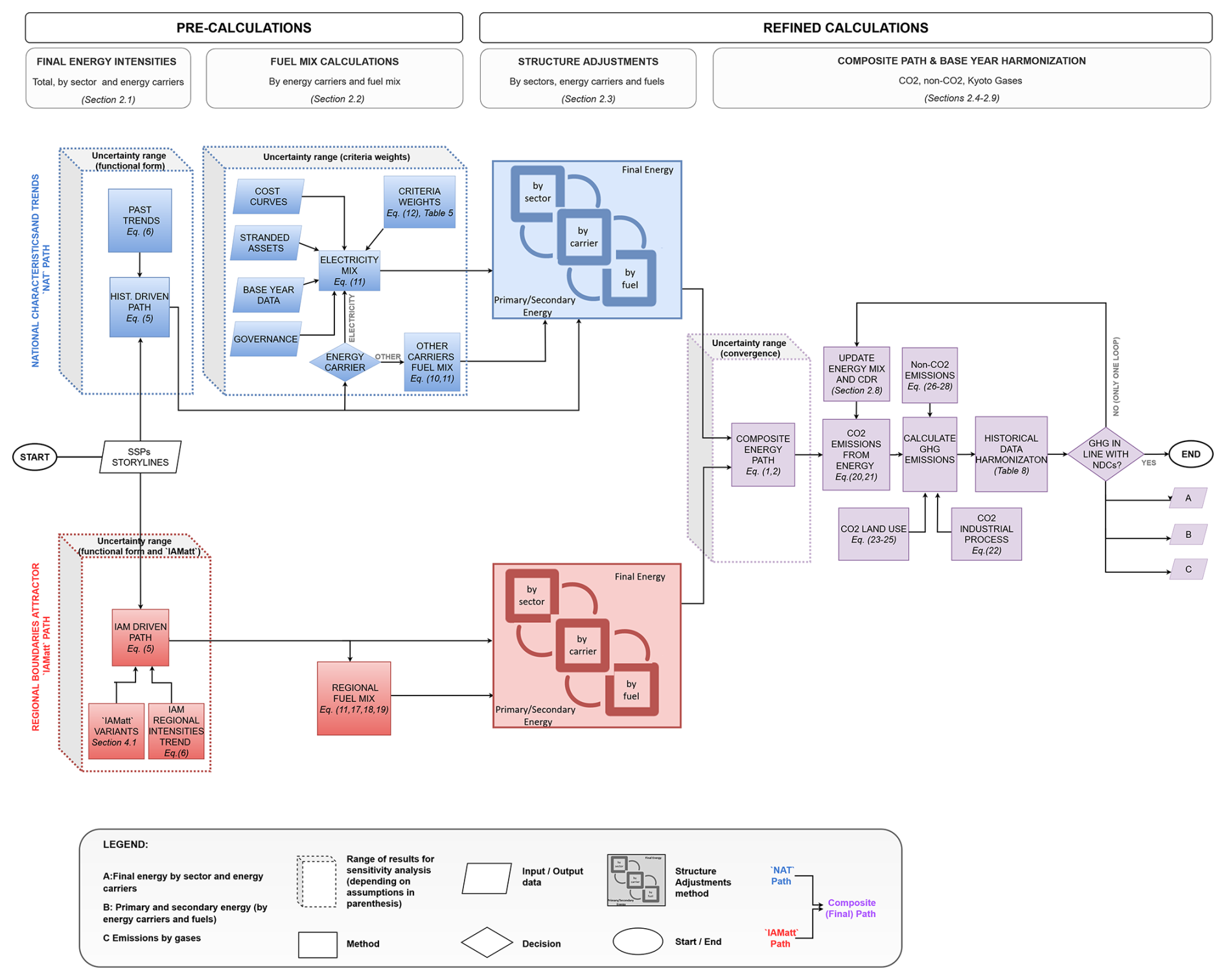
Figure 1 Flow-diagram of the downscaling algorithm (with reference to sections or equations in parentheses). The diagram shows two parallel calculations for the “NAT” path (in blue) and the “IAMatt” path (in red). These two paths are then merged in a range of “composite” paths (in purple), depending on assumptions on the timing of convergence. The “cubes” highlight further uncertainty ranges in the downscaled results (see sensitivity analysis).

Figure 1 provides an overview of how the “NAT” and “IAMatt” paths are combined into a “composite” path. The figure distinguishes between pre-calculations and refined calculations. Pre-calculations aim at projecting total final energy demand, as well as its sectors (buildings, transportation, and industry) and energy carriers (solids, liquids, gases, electricity, etc.) without ensuring consistency among them. Conversely, the refined calculations introduce some “structure adjustments”, aiming at aligning the sum across sectors, energy carriers and fuels (coal, gas, oil, etc.) in a consistent manner, in each country. After this “structure” adjustments, the “NAT” and “IAMatt” paths are merged into a “composite” path. The “composite” path calculates total GHG emissions, while considering country-level policies. Finally, it harmonizes emissions with historical country-level data until 2020, including indirect LULUCF emissions (Grassi et al., 2021) (see historical harmonization section for further details).

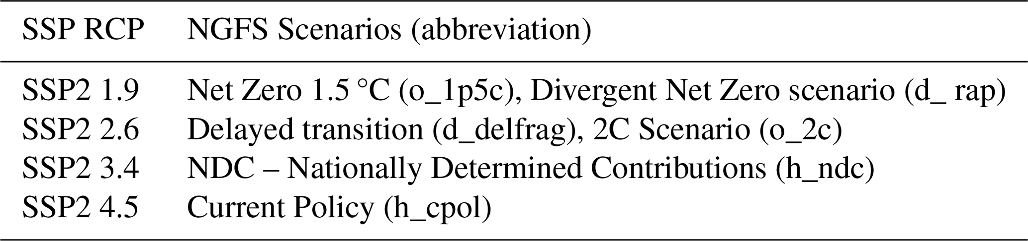
Varying the timing of convergence, as well as other downscaling assumptions (see sensitivity analysis section), allows DSCALE to provide a range of paths in each country (all of them consistent with regional IAMs results). In the context of the NGFS 2023 project, we have provided a single path based on default parameters. In our default parametrization settings, the convergence from the “NAT” path to “IAMatt” path is tailored to the narrative of a given scenario: for scenarios compatible with 1.5 °C we assume a faster convergence across countries, while convergence is slower for scenarios in line with current policy or NDCs.

Table 1 Timing of convergence and SSP storyline. “tc” refers to the time of convergence which is specific for Final Energy (FEN), secondary energy (SEN) and primary energy (PEN) variables.

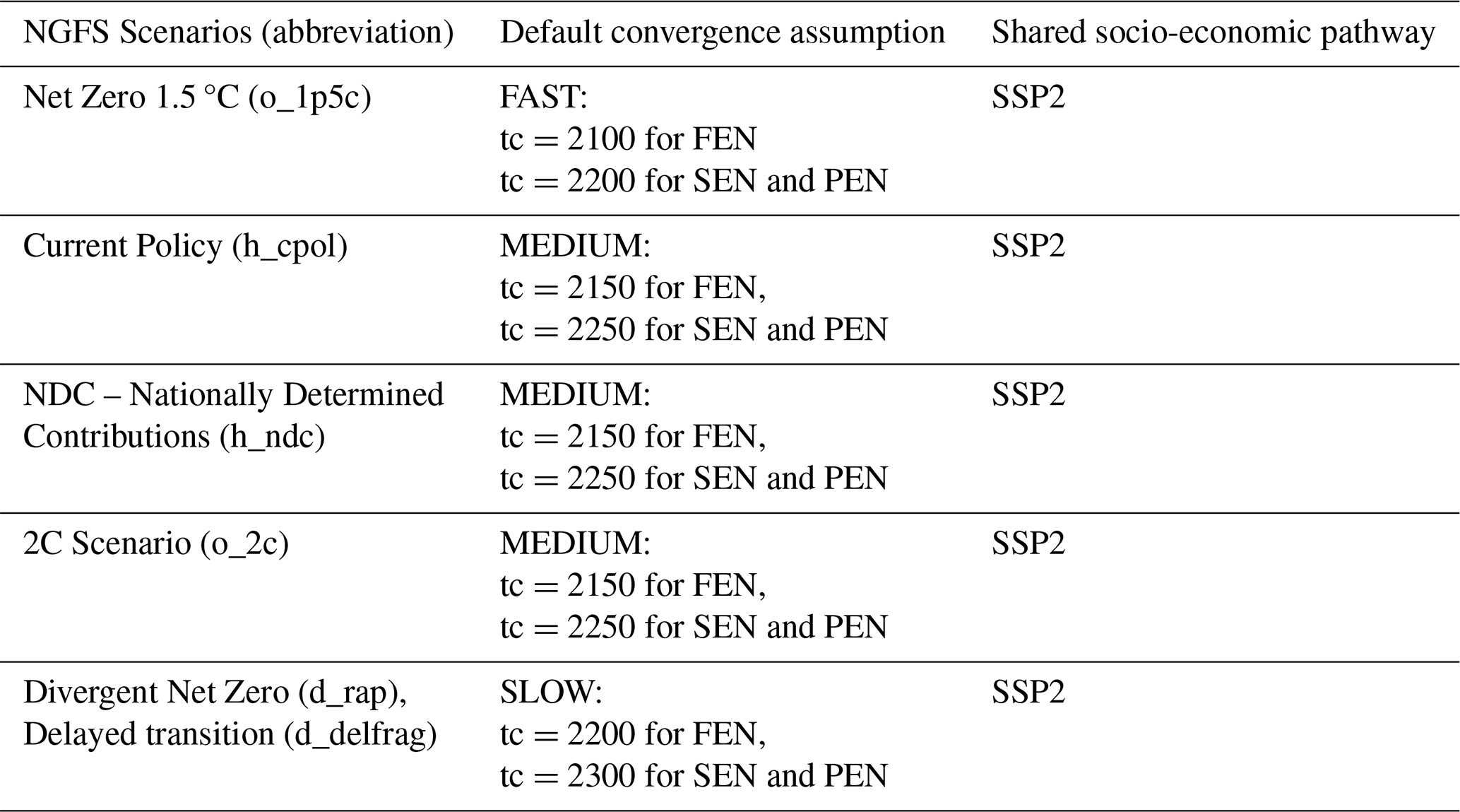
In terms of the equations, we calculate the “composite” path as a weighted average between the “NAT” and “IAMatt paths, with weight ∅ ranging from zero to one. At the base year (t0), the weight ∅ is set to one, as we rely entirely on nationally driven paths. In contrast, as time progresses and go beyond the time of convergence (tc), the weight ∅ reaches zero, leading us to exclusively utilize the “IAMatt” path. During all intermediate time steps (from t0 to tc), we calculate a weighted average as shown in Eq. (1):

$$\begin{array}{}\text{(1)}& {\displaystyle }{\mathrm{output}}_{t,c,s,e,\mathrm{tc}}={\mathrm{\varnothing }}_{t,\mathrm{tc}}{\mathrm{NAT}}_{t,c,e,s}+\left(\mathrm{1}-{\mathrm{\varnothing }}_{t,\mathrm{tc}}\right){\mathrm{IAMatt}}_{t,c,e,s}\text{(2)}& {\displaystyle }{\mathrm{\varnothing }}_{t,\mathrm{tc}}=\max \left(\mathrm{0},{\displaystyle \frac{{\mathit{\gamma }}_t-{\mathit{\gamma }}_{\mathrm{tc}}}{{\mathit{\gamma }}_{t\mathrm{0}}-{\mathit{\gamma }}_{\mathrm{tc}}}}\right)\end{array}$$

To avoid cumbersome notations, we assume that regional results are sourced from a single model and a specific scenario. Therefore, we intentionally omit these indices from the equations. In Eq. (2), weights will linearly change over time from the base year t0 until the timing of convergence and will be the same across all countries c belonging to a given region R. We constrain the weight as a positive variable ranging from one (at the base year) to zero (at the time of convergence and beyond).

2.1 Final Energy

Final energy consumption (“FEN”) is the energy (“EN”) delivered to consumers for end-use consumption. Total final energy can be decomposed into contributing factors by using a Kaya identity approach (Nakicenovic et al., 2000).

$$\begin{array}{}\text{(3)}& {\mathrm{FEN}}_{t,c,E,S}={\displaystyle \frac{{\mathrm{FEN}}_{t,c,E,S}}{{\mathrm{GDP}}_{t,c}}}{\displaystyle \frac{{\mathrm{GDP}}_{t,c}}{{\mathrm{POP}}_{t,c}}}{\mathrm{POP}}_{t,c}\end{array}$$

Total final energy is the sum of energy used across all sectors “s” and for all energy carriers “e” (in Eq. 3, they are both reported in capital letters to indicate the sum). According to Eq. (3), total final energy is driven by three contributing elements: energy intensity (final energy divided by the Gross Domestic Product “GDP”), GDP per capita and population (“POP”).

The energy intensity is a standardised metrics that allows for comparing how energy is used to produce services and final goods (hence GDP) across countries.

The DSCALE algorithm employs exogenous Population and GDP per capita pathways, based on SSP (Shared-Socioeconomic Pathways) framework (Riahi et al., 2017a). Equation (3) can be simplified by removing population (POP):

$$\begin{array}{}\text{(4)}& {\mathrm{FEN}}_{t,c,E,S}={\displaystyle \frac{{\mathrm{FEN}}_{t,c,E,S}}{{\mathrm{GDP}}_{t,c}}}{\mathrm{GDP}}_{t,c}\end{array}$$

Equation (4) can be generalized by representing final energy variable as the product of an intensity indicator “I” and an activity indicator “Q”, as shown in Eq. (5):

$$\begin{array}{}\text{(5)}& {\mathrm{FEN}}_{t,c}={\mathrm{I}}_{t,c}{\mathrm{Q}}_{t,c}\end{array}$$

At this stage, Eq. (5) intentionally omits the energy carriers (e) and sectors (s) indices, as we aim at presenting a general framework that can be used to downscale various final energy variables, by changing the corresponding activity and intensity indicators, as outlined in Table 2. When downscaling total energy demand, the activity indicator “Q” coincides with the GDP, whereas the intensity indicator “I” represents how much energy is used per unit of GDP for the overall economy (hence the energy intensity). For more detailed equations (including all indices), please refer to the Supplement (Sect. S2.5).

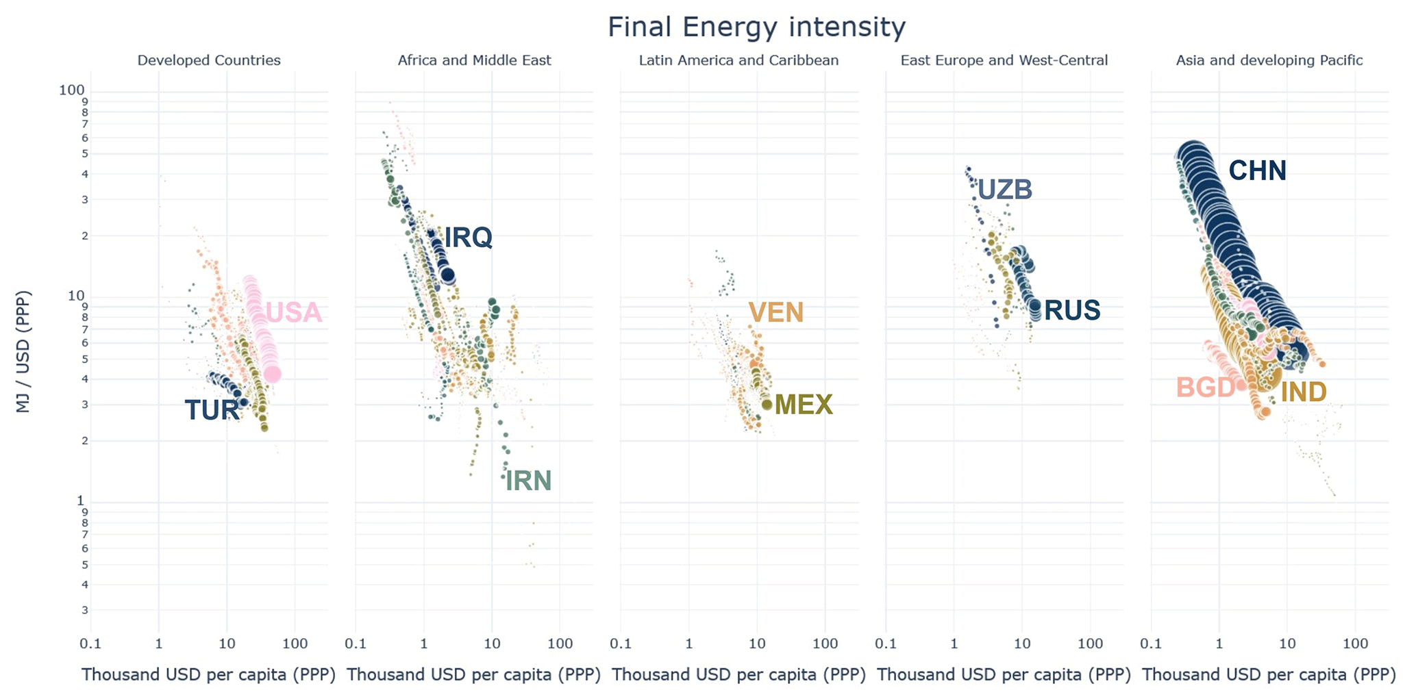
Figure 2 Historic Final Energy intensity (defined as toral final energy divided by GDP | PPP) against GDP per capita (calculations based on data from IEA energy balances from 1972–2017), across four continents (panels) and countries (coloured dots), using a log-log scale. The size of each dot is proportional to the population in each country.

To calculate total final energy demand, we need to make assumptions about the future evolution of the energy intensity over time. Historical data show that the energy intensity tends to increase in the early phases of industrialisation as traditional (non-commercial) forms or energy are replaced by commercial (and more efficient) energy. Then, the energy intensity starts to decline again as soon as this transition to commercial energy is completed – a pattern known as the hill of energy intensity (Energy Primer, 2021). Apart from this “peak”, a general downward trend dominates the historical energy intensity as income per capita increases, as shown in Fig. 2.

The literature suggests that the energy intensity can still improve by a factor ten or more in the very long term (Energy Inefficiency in the US Economy, 2024; Energy Primer, 2021; Nakicenovic et al., 1990, 1998; Nakićenović et al., 1993). Hence, we assume that this relationship between energy intensity and income per capita will continue in future long-term scenarios, by using a log-log model. The relationship between the energy intensity (represented by the intensity indicator I) and GDP per capita can be determined by regression using data from regional IAM scenarios or from historical country-level data. In the first case we obtain the “IAMatt” path, in the latter case we get the nationally driven “NAT” path. The rationale behind it is that changes in the energy intensity “I” are driven by changes in GDP per capita, as observed in historical data, and envisioned by future IAM scenarios. This means that convergence in the energy intensity across countries is conditional on the level of economic development (measured as GDP per capita) as shown in Eq. (6):

$$\begin{array}{}\text{(6)}& {\mathrm{I}}_{t,c}=\left\{\begin{array}{l}\exp \left[\mathit{\alpha }+\mathit{\beta }\log \left(\frac{{\mathrm{GDP}}_{t,c}}{{\mathrm{POP}}_{t,c}}\right)\right]\text{if\hspace{0.17em} path}=\mathrm{IAMatt}\\ \exp \left[{\mathit{\alpha }}_c+{\mathit{\beta }}_c\log \left(\frac{{\mathrm{GDP}}_{t,c}}{{\mathrm{POP}}_{t,c}}\right)\right]\text{if\hspace{0.17em} path}=\mathrm{NAT}\end{array}\right.\end{array}$$

We estimate the parameters of the functional form (the constant α and the slope β) based on historical data at the country level for the “NAT” path. Conversely, in the “IAMatt” path we estimate the parameters using regional IAM scenario results, where all countries c belonging to a region “R” will share the same α and β values.

It is important to note that the intensity indicator “I” corresponds to the energy intensity when calculating total final energy demand. However, when calculating final energy by energy carriers (and end-use sectors), “I” should be interpreted as a percentage share (e.g. the percentage share of electricity) on total energy demand “Q”.

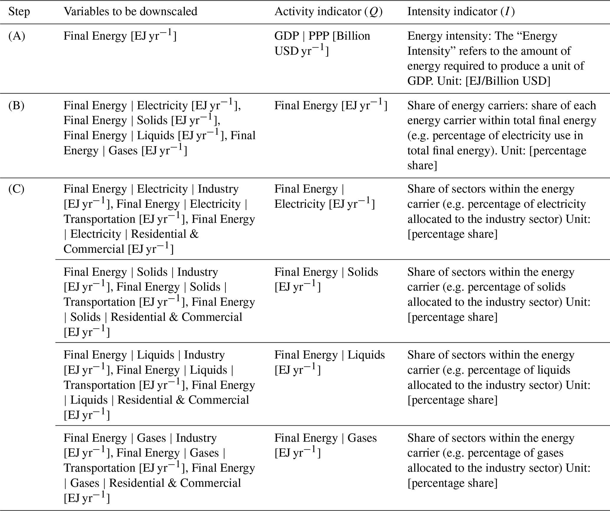
Therefore, we rely on the same approach to downscale final energy results for all the sub-sectors including different energy carriers (electricity, solids, liquids, gas) and end-use sectors (transportation, industry, residential and commercial). To do so, we employ on a hierarchical framework: first we downscale the total final energy (step A), by using GDP as the activity variable “Q” and the energy intensity as the intensity indicator “I”. In a subsequent step (B), we allocate final energy across energy carriers (liquids, solids, gases, electricity), by multiplying a percentage share “I” by an activity indicator “Q” (total final energy demand). Finally (in step C), we allocate energy consumption by energy carriers to the end use sectors (industry, transportation, residential & commercial). A full description of “Q” (activity) and “I” (intensity) indicators across all downscaling steps is provided in Table 2, whereas more detailed equations across all downscaling steps are provided in the Supplement (Sect. S2.5).

Table 2 Overview of downscaling steps (from A to C), associated variables to be downscaled, and their respective underlying activity “Q” and intensity indicators “I”. Units are indicated in square brackets.

This hierarchical approach allows a consistent downscaling of energy demand across carriers and sectors while preserving realistic system boundaries. Additional regional constraints derived from IAMs are applied during the “structural adjustments” phase, as explained in Sect. 2.3.

Finally, we apply Eq. (1) to calculate a “composite” path from the “NAT” and “IAMatt” paths using a time of convergence tc. The time of convergence is scenarios specific, with faster convergence in case of Net Zero 1.5 °C scenarios in line with the Paris Agreement, and a slower convergence for current policy scenario. This convergence process applies to final, secondary primary and energy related CO₂ emissions variables and it happens gradually over time (t). For the period between 2010 and the time of convergence tc (e.g., 2150 in our default setting), the final country-level energy intensities are calculated as a linear combination of two paths: “IAMatt” and “NAT”. The weighting between these two paths works as follows:

At the base year, the “NAT” path is weighted fully (weight =1), and the “IAMatt” path has zero weight.

Over time, the influence of the “NAT” path linearly declines to zero by the convergence year (tc), after which the “IAMatt” path fully determines the projections.

For final energy variables, this convergence process is conditional on income per capita, because the intensity indicator “I” is estimated against GDP per capita (see Eq. 6). This means that even after full convergence (beyond the time of convergence tc), countries at different income levels will retain different energy intensities, depending on the slope β of Eq. (6). For illustrative purposes, Fig. 3 shows three distinct final energy intensities (defined as total final energy divided by GDP), using a tc (time of convergence) equal to 2050, 2100, 2150, for each country of the Pacific OECD region of MESSAGE, all of them consistent with a 1.5 °C scenario.

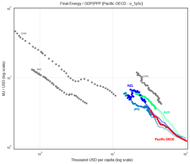
Figure 3 Downscaled total final energy intensity. Historical data are represented by dotted lines, while future downscaled data are shown as continuous coloured lines. The red line represents the Pacific OECD region from the MESSAGE model, according to a 1.5 °C pathway from 2010 to 2100. The graph displays a range of downscaled results for New Zealand (blue lines), Japan (light blue), and Australia (green lines) under different “tc” (time of convergence): 2050, 2100, 2150. Historical data for China, India, and the USA are shown only for comparison purposes and are depicted in grey, as these countries are not part of the Pacific OECD region.

In addition, the timing of convergence tc of final energy variables can be also informed by the robustness of historical trends (e.g. the r-squared of the regression) across each country and each variable. Therefore, we enhance this convergence process by applying a slower convergence when the quality of historical data in a given country is good (e.g. a long historical time series with a high R-squared), and a faster convergence when the quality is poor (e.g. a short historical time series, a low r-squared or when historical trends are in sharp contrast with future IAMs scenarios). Further details on this convergence process are provided in the Supplement.

Finally, we normally rely on a linearized “log-log” model to estimate the energy intensities trends over GDP per capita. However, different functional forms can be used, leading to different results. The sensitivity analysis section (4.1.1) will compare the results of a linearized log-log model with a logistic (s-shaped) model.

2.2 Secondary Energy

Secondary energy is source of energy that has been transformed or refined to become electricity or other energy carriers such as, liquids, solids, gases, heat, or hydrogen. Therefore, there are two dimensions associated with secondary energy: the energy carrier “e” (e.g. Electricity) and its fuel “f” composition (e.g. natural gas, oil, solar etc.). This section describes the methodology for downscaling secondary energy variables “SEN” by energy carrier and fuel.

As a general framework, secondary energy variables will build upon previously downscaled final energy variables, available for each energy carrier.

As a first step, we calculate secondary energy from final energy FEN, assuming the same conversion factors of regional IAMs results. This factor is defined as the ratio between secondary and final energy data from regional IAMs results, hence reflecting trade and distribution losses.

$$\begin{array}{}\text{(7)}& {\mathrm{SEN}}_{t,c,e}={\mathrm{FEN}}_{t,c,e}{\displaystyle \frac{{\mathrm{SEN}}_{t,R,e}}{{\mathrm{FEN}}_{t,R,e}}}\end{array}$$

Regarding the fuel composition across energy carriers, we apply different approaches for the “NAT” and “IAMatt” paths. The “NAT” path relies on historical country-level data as the main downscaling criteria, using the share of country within the region (“histratio”) at the base year (“t0”). For example, if a given fuel (e.g. Liquids | Oil) will be phased out at the regional level at a future point in time (e.g. 2030), the same will happen in all countries c belonging to the region R. This approach works if historical data is available for a given fuel. If data is not available (or equal to zero), we will rely solely on “IAMatt” path. This could be the case for technologies that are relatively expensive today (and therefore rarely used) but that could become cheaper in the future, depending on the scenario considered (e.g. Coal to Liquids).

In the “IAMatt” path, we downscale secondary energy at the country level assuming the same fuel composition observed at the regional level for each energy carrier (e). For instance, if solar energy accounts for 50 % of electricity generation at any given point in time, the same will apply across all countries in that region. This approach is more suitable in the long-term, as it heavily depends on scenario narratives. Disruptive scenarios, such as those involving stringent temperature targets, may significantly alter the current energy mix in the long term.

$$\begin{array}{}\text{(8)}& {\displaystyle }{\mathrm{SEN}}_{t,c,e,f}=\left\{\begin{array}{l}\frac{{\mathrm{SEN}}_{t,R,e,f}}{{\mathrm{SEN}}_{t,R,e}}{\mathrm{SEN}}_{t,c,e}\text{if\hspace{0.17em} path}=\text{IAMatt}\\ {\mathrm{SENnat}}_{t,c,e,f}\text{if\hspace{0.17em} path}=\text{NAT}\end{array}\right.\text{(9)}& {\displaystyle }{\mathrm{SENnat}}_{t,c,e,f}=\left\{\begin{array}{l}{\mathrm{EL}}_{t,c,e,f}\text{if}e=\text{electricity}\\ {\mathrm{SEN}}_{t,R,e,f}{\mathrm{histratio}}_{c,e,f}\text{otherwise}\end{array}\right.\end{array}$$

So far, we have presented the general framework for downscaling secondary energy liquids, solids and gases. However, when downscaling the electricity sector (EL), it is worth using a variety of criteria on top of historical data to determine the “NAT” path. These criteria include the age of fossil-fuel based power plants, the role of public institutions to support technologies like nuclear or provide incentives for renewables energy. The methodology for downscaling the “NAT” path of the electricity sector (EL), is described in the Sect. 2.2.1.

2.2.1 Secondary Energy Electricity (“NAT” path)

For the “NAT” path we use historical data to initialize the electricity mix at the base year “t0” in each country, by relying on the same approach used for liquids, solids, and gases. For subsequent years, the electricity mix in can be determined by using a variety of criteria (i) as described in Table 3.

Table 3 Additional criteria.

$$\begin{array}{}\text{(10)}& {\displaystyle }{\mathrm{histratio}}_{c,e,f}={\displaystyle \frac{{\mathrm{SEN}}_{t\mathrm{0},c,e,f}}{{\sum }_c{\mathrm{SEN}}_{t\mathrm{0},c,e,f}}}\text{(11)}& {\displaystyle }{\mathrm{ELnat}}_{t,c,e,f}=\left\{\begin{array}{l}{\mathrm{SEN}}_{t,R,e,f}{\mathrm{histratio}}_{c,e,f}\text{if}t=t_{\mathrm{0}}\\ {\mathrm{ELnat}}_{t+\mathrm{1},c,e,f}={\mathrm{ELnat}}_{t,c,e,f}\text{or}e\ne \text{electricity}\\ +\mathrm{\Delta }{\mathrm{SEN}}_{t,R,e,f}{\sum }_i{\mathit{\omega }}_i\frac{{\mathrm{ELI}}_{t,c,e,f,i}}{{\sum }_c{\mathrm{SEN}}_{t,R,e,f,i}}\text{otherwise}\end{array}\right.\text{(12)}& {\displaystyle }{\mathrm{ELI}}_{t,c,e,f,i}=\left\{\begin{array}{ll}{\mathrm{histratio}}_{c,e,f}& \forall f\mathit{ϵ}F\text{and}i=\text{histdata}\\ \frac{{\mathrm{GOV}}_{t,c,e,f}}{{\mathrm{GOV}}_{t,R,e,f}}& \forall t\ge t_{\mathrm{0}}\forall f\mathit{ϵ}\left[\text{wind,\hspace{0.17em} solar,\hspace{0.17em} nuclear}\right]\\ & \text{and}i=\text{governance}\\ \frac{{\mathrm{GW}}_{t,c,e,f}}{{\mathrm{GW}}_{t,R,e,f}}& \forall t\ge t_{\mathrm{0}}\forall f\mathit{ϵ}\left[\text{coal,\hspace{0.17em} gas,\hspace{0.17em} oil,\hspace{0.17em} geothermal}\right]\\ & \text{and}i=\text{strandedassets}\\ \frac{{\mathrm{MC}}_{t,c,e,f}}{{\mathrm{MC}}_{t,R,e,f}}& \forall t\ge t_{\mathrm{0}}\forall f\mathit{ϵ}\left[\text{wind,\hspace{0.17em} solar,biomass,\hspace{0.17em} hydro}\right]\\ & \text{and}i=\mathrm{costcurves}\end{array}\right.\end{array}$$

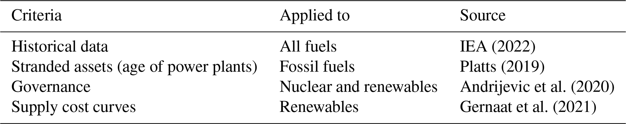
The historical data criterion is generally applicable to all fuels, as it allocates fuel based on historical data at the base year. It is essentially the method described by Eqs. (9) and (10) for the liquids, solids, and gases.

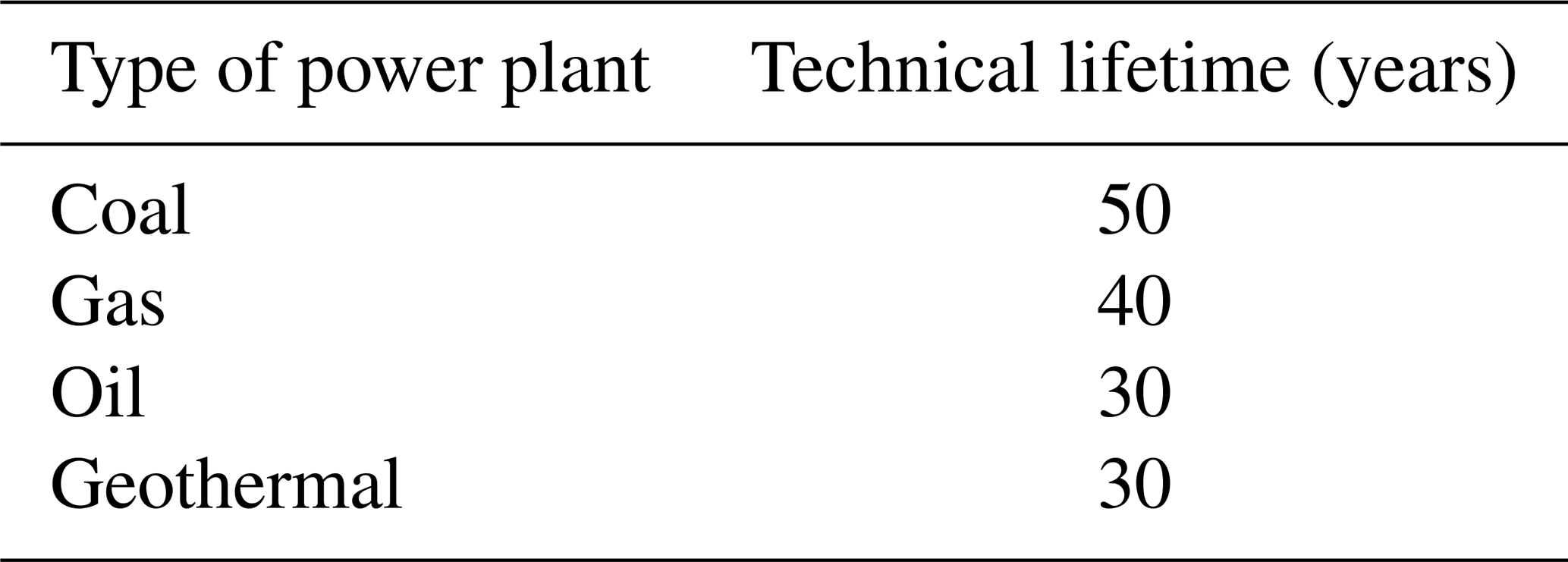
The stranded assets minimization criterion calculates the remaining technical lifetime of fossil fuel-based power plants in each country using the PLATTS database (2019). It assumes that existing and planned power plants at the country level are preferred over building new power plants, to avoid costly carbon lock-in. If the expected retirement date from the PLATTS database is unknown, we use the assumptions reported in Table 4 about the technical lifetime.

Table 4 Technical lifetime assumptions if retirement date is missing in the PLATTS database.

Based on the expected retirement date and new power plants (planned or under construction), we project the future installed capacity at the country level for each fossil fuel (f) at the country level. Then we allocate electricity generation for each fuel at the country level based on projected capacity (GW), as shown in Eq. (12) (i= strandedassets).

Another criterion used for downscaling low-carbon technologies is governance. Country level projections of governance indicators are available for different SSP storylines (Andrijevic et al., 2020). We use these indicators as proxy for allocating regional nuclear power plants and renewable energy developments to the country level. The main rational behind this is that countries investing in low-carbon technologies require support from institutions, which is more likely to happen in countries with higher level of governance. Investing in critical technologies like nuclear may require stable long-term support from public institutions. Intermittent renewables may also require overhaul of electricity grids, in the long term, which are normally controlled by the state. In this context, governance benchmarks are useful indicators to assess capacity to invest in low-carbon technologies.

The availability of renewables (e.g. solar energy) is not distributed evenly across countries. Supply cost curves can be used to capture the availability of energy supply at a given cost. For renewable energy we rely on supply cost curves to allocate electricity generation based on cost minimization and available potential (Gernaat et al., 2021). To this end, we rank each country by cost and allocate renewables based on the associated potential at the country level. We use supply cost curves to determine country level production associated to a given regional production (based on IAMs). A limitation of this approach is that supply cost curves provide only a static representation of energy availability and costs, overlooking path dependency, uncertainty, and system-wide interactions.

The choice of criteria for downscaling yields diverse results for the electricity mix. We can select criteria with weights ranging from zero (not considered) to one (fully considered). In our default parameterization, we employ weights for criteria as reported in Table 5.

Table 5 Default criteria weights across different fuels in the electricity sector.

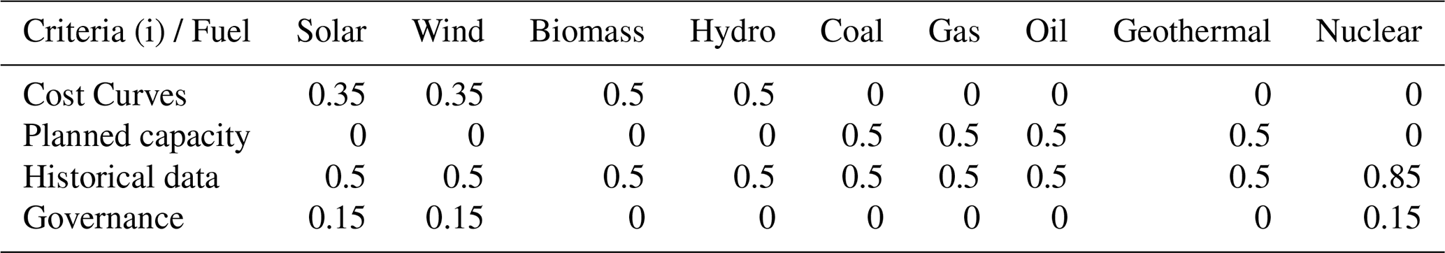
For biomass and hydro, we apply an equal weighting of 50 % on historical data and 50 % on supply cost curves, as these energy sources are typically concentrated in specific countries with favourable natural conditions. On the one hand historical data capture the role of existing infrastructures. On the other hand, the resources availability and economic potential are reflected in supply cost curves, with the aim of enhancing the future allocation of these resources across countries.

For solar and wind, the weights distribution aims at capturing current infrastructures (historical data, 50 %), future economic potential (supply cost curves, 35 %) as well as support from public institutions (governance indicators, 15 %). Historical data (50 %) serves as the primary driver in the short term, capturing real-world availability data, shaped by past policy support and market conditions. Supply cost curves reflect each the long-term economic potential for solar and wind deployment in each country. These curves mimic the outcomes of a cost-minimization process, showing where renewables are likely to develop if solely driven by cost efficiency. However, supply curves can produce somewhat abrupt or “stepwise” behaviours, especially when technologies only appear in countries where costs fall below specific thresholds. This makes them less reliable for capturing early-stage deployment patterns, and for this reason we assign to them a lower weight (35 %, compared to historical data weight of 50 %). Finally, governance indicators reflect the enabling role of institutions in supporting renewables including financial incentives. However, they do not directly reflect physical or economic resource availability, hence we apply a smaller weight (15 %).

For coal, gas, oil, and geothermal, we equally apply historical data and remaining technical lifetime (50 % each) as criteria weights for the downscaling. The rationale is that the future distribution of conventional power generation capacity is strongly influenced by both historical patterns of energy production (providing a baseline for near-term allocation) and remaining operational lifetimes (including announced/planned new capacities). Older plants nearing end-of-life may be phased out sooner, while newer facilities with more remaining capacity are likely to operate longer.

For nuclear, we set the weights at 85 % for historical data and 15 % for governance Indicators, with the aim of reflecting path-dependencies and political sensitivity associated with nuclear development. We use historical data as the main criteria to allocate nuclear energy developments to the country level. However, governance indicators remain a relevant factor, as only countries with high institutional and regulatory capacity are likely to pursue or expand nuclear power programs.

Finally, since governance indicators, economic lifetime and supply cost curves do not necessarily reflect the historical electricity mix, at the base year, we initialise electricity generation by using the historical data criteria, in t0. Then we introduce some path dependencies in the development of the electricity mix over time, as shown in Eq. (11). This dynamic update ensures a smooth transition, while allowing for gradual shifts from the base year to future long-term scenarios. This is especially relevant under scenarios with stringent climate targets. However, it should be noted that rapid changes could still occur in the short term. A typical example is the situation of a small island that heavily relies on oil-based power plants for its energy need, while this technology is phased out at the regional level (replaced by more efficient and cheaper technologies).

2.3 Structure adjustments

Downscaled results need to be plausible and internally consistent (Grübler et al., 2007). To this end, we introduce a “structure adjustments” approach by using an iterative process:

• first, we re-scale the structure of each variable in a proportional manner, so that the sum of sectors (s) and energy carriers (e) is aligned with total final energy demand within each country.

• Second, we update the energy variables so that the sum across countries matches the regional IAMs results.

The first step in this process aligns the sum of sectors (s) with total final energy in each country, as shown in Eq. (13).

$$\begin{array}{}\text{(13)}& \widehat{{\mathrm{FEN}}_{t,c,e,s}}={\mathrm{FEN}}_{t,c,e,s}{\displaystyle \frac{{\mathrm{FEN}}_{t,c,E,S}}{{\mathrm{FEN}}_{t,c,e,S}}}\end{array}$$

Equation (13) introduces a “top-down” harmonization because each sector is scaled up or down proportionally, to match total final energy demand (FEN${}_{t,c,E,S}$). For example, if total final energy demand is 10 % higher than the sum across sectors (FEN${}_{t,c,e,S}$) in a given country, each sector will be multiplied by 1.1. In this manner, the sum of industry, transportation and residential & commercial will match total final energy demand, in each country.

The updated results from Eq. (13) are denoted with a “wide hat”, indicating that the sum of country level results may not be any longer consistent with the regional IAMs results. To overcome this problem, we introduce another Eq. (14) which brings back consistency with regional IAMs results

$$\begin{array}{}\text{(14)}& {\mathrm{FEN}}_{t,c,e,s}=\widehat{FE{N}_{t,c,e,s}}{\displaystyle \frac{{\mathrm{FEN}}_{t,R,e,s}}{{\sum }_c\widehat{{\mathrm{FEN}}_{t,c,e,s}}}}\end{array}$$

Equation (14) aligns the sum across countries with regional IAMs results in a proportional manner. For example, if the sum across countries is 5 % higher than regional IAMs results, the results will be scaled down by 5 %, to bring back consistency.

At this point, we have updated final energy results by sector, so that their sum is consistent with the total final energy in each country, as shown in Eq. (13). At the same time, we ensure that the sum of country level results still match the regional IAMs results, by applying Eq. (14). In a similar way we should ensure that the sum of energy carriers is aligned with the total final energy. And the same should hold true not just for total final energy, but also for the other sub-categories. For example, “Final Energy | Liquids” should coincide with the amount of liquids used in the transportation, industry, and residential and commercial sectors.

We apply these two equations for all sectors and energy carriers, using the hierarchical steps (from large to small sectors) as shown in Table 6.

Table 6 Default criteria weights across different fuels in the electricity sector.

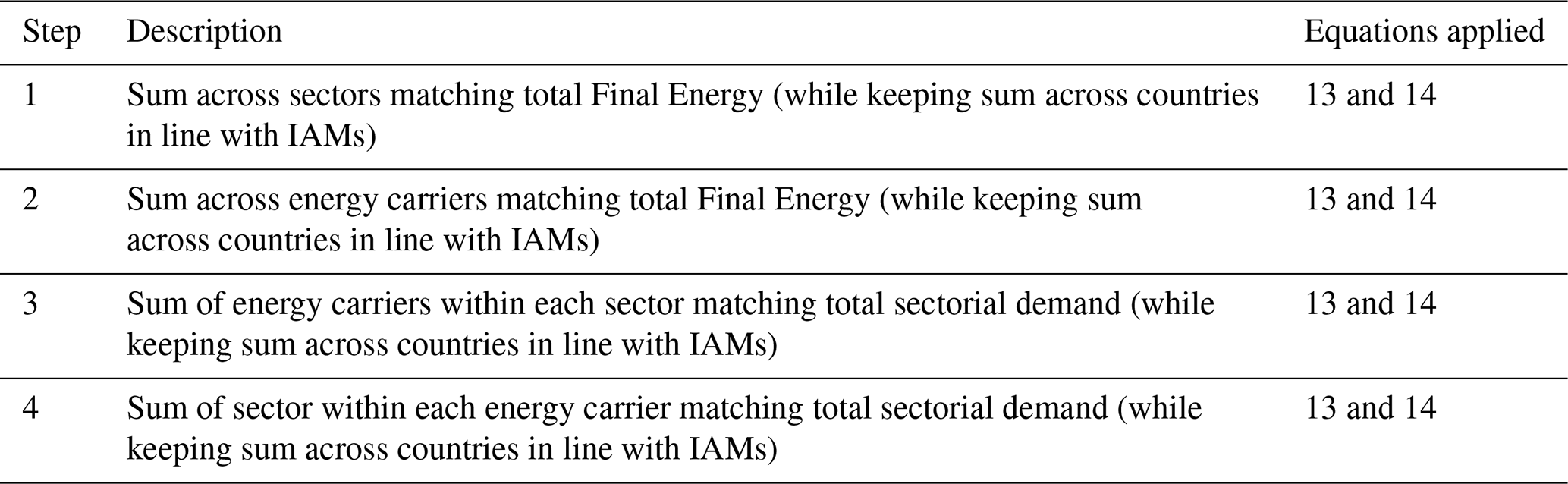
We iterate along these steps for all final energy variables, in order to reach a stable solution. Then, we calculate a range of “composite” paths depending on the timing of convergence tc (using Eq. 1).

Electricity trade minimization

The downscaling algorithm aims at minimizing trade and electricity losses across countries within the region, in order to avoid unrealistic trade patterns in the long term. Trade and electricity losses can be computed as the difference between final (FEN${}_{t,c,e}$) and total secondary energy (SEN${}_{t,c,e,F}$), where e= electricity. We minimize trade and distribution losses by aligning secondary energy to total final energy electricity in each country, as shown in Eq. (15):

$$\begin{array}{}\text{(15)}& \widehat{{\mathrm{SEN}}_{t,c,e,f}}={\mathrm{SEN}}_{t,c,e,f}{\displaystyle \frac{{\mathrm{FEN}}_{t,c,e}}{{\mathrm{SEN}}_{t,c,e,F}}}\end{array}$$

Equation (15) aligns secondary energy (SEN) with total final energy demand (FEN) for each energy carrier(e), with the aim of minimizing trade and transmission and distribution losses. However, this equation breaks consistency between the sum across countries and the regional IAMs results. Equation (16) is then applied to restore this consistency.

$$\begin{array}{}\text{(16)}& {\mathrm{SEN}}_{t,c,e,f}=\widehat{{\mathrm{SEN}}_{t,c,e,f}}{\displaystyle \frac{{\mathrm{SEN}}_{t,R,e,f}}{{\sum }_c\widehat{{\mathrm{SEN}}_{t,c,e,f}}}}\end{array}$$

By iterating Eqs. (15) and (16) we minimize trade and electricity losses across all countries within the region, while keeping consistency with regional IAMs results.

2.4 Primary energy and related carbon emissions

Primary energy (“PEN”) refers to the energy contained in natural resources, such as natural gas and oil, that has not undergone any human-made conversion processes. This section describes the methodology used to downscale primary energy by fuel.

To calculate the primary energy mix at the country level we multiply secondary energy by a conversion factor. To ensure consistency with regional result, we use the same conversion factor used by IAMs:

$$\begin{array}{}\text{(17)}& {\mathrm{PEN}}_{t,c,E,f}={\mathrm{SEN}}_{t,c,E,f}{\displaystyle \frac{{\mathrm{PEN}}_{t,R,E,f}}{{\mathrm{SEN}}_{t,R,E,f}}}\end{array}$$

Some fuels can be coupled with CCS (Carbon Capture and Storage) technologies, able to store most of the emissions underground. While calculating emissions we assume a capture rate of 90 % for CCS technologies. Therefore, we distinguish between technologies “w/CCS” and “w/o” CCS by applying the same percentage ratio observed in regional IAMs results to the country level.

$$\begin{array}{}\text{(18)}& {\displaystyle }{\mathrm{PEN}}_{t,c,E,f_{w/ccs}}={\mathrm{PEN}}_{t,c,E,f}{\displaystyle \frac{{\mathrm{PEN}}_{t,R,E,f_{w/ccs}}}{{\mathrm{PEN}}_{t,R,E,f}}}\text{(19)}& {\displaystyle }{\mathrm{PEN}}_{t,c,E,f_{w/o}}={\mathrm{PEN}}_{t,c,E,f}{\displaystyle \frac{{\mathrm{PEN}}_{t,R,E,f_{w/o}}}{{\mathrm{PEN}}_{t,R,E,f}}}\end{array}$$

We calculate energy related CO₂ emissions by applying emissions factors to the energy mix (including negative emission factor from BECCS derived from regional IAMs results and a 10 % leakage from fossil fuels technologies with CCS):

$$\begin{array}{}\text{(20)}& \widehat{{\mathrm{CO}\mathrm{2}\mathrm{EN}}_{t,c}}=\sum _f{\mathrm{PEN}}_{t,c,f}{\mathrm{EF}}_{t,c,f}\end{array}$$

CO₂ emissions from energy (CO2EN) are denoted with a “wide hat”, highlighting possible mismatches between the sum of country level results and regional IAMs results. Therefore, we harmonize the energy related CO₂ emissions to ensure consistency with regional IAMs scenarios.

$$\begin{array}{}\text{(21)}& \mathrm{CO}\mathrm{2}{\mathrm{EN}}_{t,c}=\widehat{\mathrm{CO}\mathrm{2}{\mathrm{EN}}_{t,c}}{\displaystyle \frac{\mathrm{CO}\mathrm{2}{\mathrm{EN}}_{t,R}}{\sum _c\widehat{\mathrm{CO}\mathrm{2}{\mathrm{EN}}_{t,c}}}}\end{array}$$

2.5 Industrial Processes

CO₂ emissions from industrial processes (“ICO2”) are emissions stemming from the creation of industrial processes that transform materials such as cement. These emissions are associated with various industrial activities, including metal, chemical, mineral, and electronics industries within each country. Hence, we downscale industrial process emissions by using final energy consumption from industry as a proxy for industrial activity. Based on the downscaled final energy results from industry (FEN, with s= industry), we allocate regional industrial CO₂ emissions from IAMs (ICO2_R) to the country level.

$$\begin{array}{}\text{(22)}& \mathrm{ICO}{\mathrm{2}}_{t,c}={\displaystyle \frac{{\mathrm{FEN}}_{t,c,s=\mathrm{industry}}}{{\mathrm{FEN}}_{t,R,s=\mathrm{industry}}}}\mathrm{ICO}{\mathrm{2}}_{t,R}\end{array}$$

2.6 Land Use

Land use emissions (“LU”) can be distinguished in direct (“LUD”) and indirect (“LUI”) emissions. Direct land use emissions are anthropogenic fluxes (due to human-induced land-use changes), whereas indirect land use emissions are the natural response of land to environmental changes (e.g. CO₂ fertilization or climate change) (Gidden et al., 2023).

IAMs usually provide results only for direct land use emissions, whereas GHG inventories cover both direct and indirect emissions. This leads to a gap of around 5.5 GtCO₂ of carbon sinks globally (Grassi et al., 2021).

While downscaling direct land use emissions from IAMs, we allocate the change in direct land use emissions over time from IAMs to the country level based on the historical standard deviation (σ) of the last 10 years, using Eq. (23):

$$\begin{array}{}\text{(23)}& {\mathrm{LUD}}_{t,c}={\displaystyle \frac{{\mathit{\sigma }}_c}{\sum _c{\mathit{\sigma }}_c}}\left({\mathrm{LUD}}_{t,R}-{\mathrm{LUD}}_{t-\mathrm{1},R}\right)+{\mathrm{LUD}}_{t-\mathrm{1},c}\end{array}$$

We use the standard deviation, as it captures both the size of emissions (in absolute terms) and the volatility in each country. As a result, changes in direct land use emissions from IAMs will be mostly allocated to countries with larger emissions and higher volatility within the region. This also means that countries with stable emissions in the past will remain relatively stable in the future.

We then downscale indirect land use emissions using Eq. (24):

$$\begin{array}{}\text{(24)}& {\mathrm{LUI}}_{t,c}={\displaystyle \frac{{\mathrm{LUI}}_{t,R}}{{\mathrm{LUI}}_{t\mathrm{0},R}}}{\mathrm{LUI}}_{t\mathrm{0},c}\end{array}$$

Considering the volatile nature of land use, we initialize the land use indirect (LUI) emissions data based on the average values from 2010–2020 from DGVMs (Dynamic Global Vegetation Models), from the non-intact forest category. We then apply the growth rates of the regional adjustment values estimated by IMAGE/LPJmL model (Grassi et al., 2021), to each country belonging to the same region. As these growth rates are influenced by global mean temperature, we map the NGFS scenario with the RCP emissions trajectory reported by Grassi and co-authors 2021, as shown in Table 7.

Table 7 NGFS Scenario mapping with the SSP/RCP framework.

Scenarios have been mapped based on the global temperature peak, as well as 2100 temperature values from the NGFS scenarios, in comparison with the SSP/RCP scenarios. Finally, we calculate total land use emissions as the sum of direct and indirect emissions, as shown in Eq. (25).

$$\begin{array}{}\text{(25)}& {\mathrm{LU}}_{t,c}={\mathrm{LUD}}_{t,c}+{\mathrm{LUI}}_{t,c}\end{array}$$

2.7 non-CO₂ emissions

This section focuses on downscaling non-CO₂ emissions, by linking regional Integrated Assessment Models (IAMs) results with the GAINS country-level model results (Höglund-Isaksson et al., 2020; Winiwarter et al., 2018). The GAINS model focuses on cost-effective strategies for greenhouse gas emissions control, emphasizing improvements in air quality. It provides non-CO₂ emissions results for baseline and maximum technical abatement potential scenarios across 96 countries. Typically, IAM scenarios fall between the GAINS baseline and maximum technical potential. To align IAMs results (at the regional level), with the GAINS model data (at the country level), we apply linear interpolation between the GAINS baseline and stabilization (maximum mitigation potential) scenario to match a given IAMs scenario at the regional level, throughout different points in time. The resulting downscaled emissions coincide with the GAINS country-level data only when IAM scenarios coincide either with the baseline (“Gbau”) or maximum abatement (“Gstab”) from GAINS.

$$\begin{array}{}\text{(26)}& \begin{array}{rl}\widehat{\mathrm{nonCO}{\mathrm{2}}_{t,c,j}}& ={\mathrm{Gbau}}_{t,c,j}+\left({\mathrm{IAM}}_{t,R,j}-{\mathrm{Gbau}}_{t,R,j}\right)\\ & {\displaystyle \frac{{\mathrm{Gbau}}_{t,c,j}-{\mathrm{Gstab}}_{t,c,j}}{{\mathrm{Gbau}}_{t,R,j}-{\mathrm{Gstab}}_{t,R,j}}}\end{array}\end{array}$$

when downscaling country-level non-CO₂ emissions, no extrapolation is applied if IAM emissions exceed the GAINS baseline or fall below the maximum technical potential:

$$\begin{array}{}\text{(27)}& \widehat{\mathrm{nonCO}{\mathrm{2}}_{t,c,j}}=\max \left[min\left(\widehat{\mathrm{nonCO}{\mathrm{2}}_{t,c,j}},{\mathrm{Gbau}}_{t,c,j}\right),{\mathrm{Gstab}}_{t,c,j}\right]\end{array}$$

The “nonCO2” emissions variable is represented with a hat, as the sum of country level outcomes is not necessarily in line with regional IAMs results. Therefore, we harmonize the emissions trajectory to ensure that the overall sum of country-level results aligns with regional IAMs data.

$$\begin{array}{}\text{(28)}& \mathrm{nonCO}{\mathrm{2}}_{t,c,j}=\widehat{\mathrm{nonCO}{\mathrm{2}}_{t,c,j}}{\displaystyle \frac{{\mathrm{IAM}}_{t,R,j}}{\widehat{\sum _c\mathrm{nonCO}{\mathrm{2}}_{t,c,j}}}}\end{array}$$

We apply this methodology to CH₄, HFC, N₂O and SF6 emissions (j index). We convert emissions in MtCO₂ eq. using IPCC GWP100 (Global Warming Potentials over a time frame of 100 years). GWP estimates vary depending on the IPCC assessment (e.g.AR4, AR5, AR6 etc.), and this can be chosen depending on the scenario to be downscaled. In our default setting, we use GWP estimates from the latest IPCC assessment (AR6.). Finally, we calculate total non-CO₂ emissions as the sum of individual non-CO₂ gases.

2.8 Introducing country-level emissions policy targets

To enhance realism of country-level projections, the downscaling algorithm can optionally incorporate GHG emissions targets at the country level, as stated in the NDCs (Nationally Determined Contributions) and LTS (Long Term Strategies). Those targets are introduced as soft constraints, to avoid possible inconsistencies with underlying IAMs scenarios. To do so, we assume that countries will try to reach their domestic targets, although they might be only partially achieved, depending on regional policies considered by a given model/scenario. To achieve this, we first compute total GHG emissions as the sum of total CO₂ emissions (including LULUCF) and total non-CO₂ gases based on IPCC GWP100 (Global Warming Potentials over a time frame of 100 years), as shown in Eq. (29).

$$\begin{array}{}\text{(29)}& {\mathrm{GHG}}_{t,c}=\mathrm{CO}\mathrm{2}{\mathrm{EN}}_{t,c}+\mathrm{ICO}{\mathrm{2}}_{t,c}+{\mathrm{LU}}_{t,c}+\sum _j\mathrm{nonCO}{\mathrm{2}}_{t,c,j}\end{array}$$

Secondly, we calculate the gap between current total GHG emissions (without policies) and the emissions targets. Then, we distribute those emissions targets (for 2030 and 2050) to yearly emissions targets for all time periods (starting from 2015), assuming that they will gradually tighten over time, based on a linear interpolation. Yearly emissions targets are denoted by GHG*:

$$\begin{array}{}\text{(30)}& {\mathrm{GAP}}_{t,c}={\mathrm{GHG}}_{t,c}^{\ast }-{\mathrm{GHG}}_{t,c}\end{array}$$

Thirdly, we assume that countries will fill the emissions gap by either increasing BECCS (Carbon sequestration from Biomass with CCS), or by replacing fossil fuels with renewables. We assume that BECCS can fill maximum of 50 % of the emissions gap, as shown in Eq. (31):

$$\begin{array}{}\text{(31)}& {\widehat{\mathrm{BECCS}}}_{t,c}={\mathrm{BECCS}}_{t,c}+\mathrm{0.5}\times {\mathrm{GAP}}_{t,c}\end{array}$$

BECCS is now shown with “wide hat” because the sum across countries is no longer consistent with regional IAMs results. To bring back consistency we apply Eq. (32):

$$\begin{array}{}\text{(32)}& {\mathrm{BECCS}}_{t,c}=\widehat{{\mathrm{BECCS}}_{t,c}}+{\displaystyle \frac{{\mathrm{BECCS}}_{t,R}}{\widehat{\sum _c{\mathrm{BECCS}}_{t,c}}}}\end{array}$$

Please note that if BECCS is not available at the regional level at a given time (e.g. 2030), it will be zero in each country, regardless of the level of ambition of their NDCs. For this reason, the contribution of BECCS can range from 0 % to 50 % of the emissions gap, depending on regional IAMs data. The development of BECCS (Carbon sequestration from biomass with CCS) affects energy related CO₂ emissions “CO2EN”. Therefore, we update “CO2EN” and then recalculate “GHG” emissions and the remaining emissions gap. This gap, which can account for 50 % or more, must be filled by reducing emissions from fossil fuels. To do so, we convert the emissions gap into an energy gap, by dividing it by an average emissions factor across all fossil fuels.

$$\begin{array}{}\text{(33)}& {\mathrm{ENGAP}}_{t,c}={\displaystyle \frac{{\mathrm{GAP}}_{t,c}}{{\mathrm{avemifactor}}_{t,c}}}\end{array}$$

Each fossil fuel will contribute to reducing this gap proportionally, based on its share. For instance, if coal accounts for 90 % of fossil fuels, it will be responsible for addressing 90 % of the energy gap.

$$\begin{array}{}\text{(34)}& {\widehat{\mathrm{EN}}}_{t,c,f}={\mathrm{EN}}_{t,c,f}-{\mathrm{ENGAP}}_{t,c}{\displaystyle \frac{{\mathrm{EN}}_{t,c,f}}{\sum _f{\mathrm{EN}}_{t,c,f}}}\forall f\in \mathrm{fossils}\end{array}$$

This also means that each fossil fuel will be reduced by the same percentage. Hence, Eq. (34) can be rewritten as:

$$\begin{array}{}\text{(35)}& {\widehat{\mathrm{EN}}}_{t,c,f}={\mathrm{EN}}_{t,c,f}\left(\mathrm{1}-{\displaystyle \frac{{\mathrm{ENGAP}}_{t,c}}{\sum _f{\mathrm{EN}}_{t,c,f}}}\right)\forall f\in \mathrm{fossils}\end{array}$$

At the same time, renewable energy will be up scaled to compensate for a reduction in fossil fuel energy.

$$\begin{array}{}\text{(36)}& {\widehat{\mathrm{EN}}}_{t,c,f}={\mathrm{EN}}_{t,c,f}+{\mathrm{ENGAP}}_{t,c}{\displaystyle \frac{{\mathrm{EN}}_{t,c,f}}{\sum _f{\mathrm{EN}}_{t,c,f}}}\forall f\in \mathrm{renewables}\end{array}$$

The same equation can be rewritten as:

$$\begin{array}{}\text{(37)}& {\widehat{\mathrm{EN}}}_{t,c,f}={\mathrm{EN}}_{t,c,f}\left(\mathrm{1}+{\displaystyle \frac{{\mathrm{ENGAP}}_{t,c}}{\sum _f{\mathrm{EN}}_{t,c,f}}}\right)\forall f\in \mathrm{renewables}\end{array}$$

EN is denoted with a “wide hat” because the sum across countries is no longer consistent with regional IAM results. To bring back consistency we apply Eq. (38):

$$\begin{array}{}\text{(38)}& {\mathrm{EN}}_{t,c,f}={\widehat{\mathrm{EN}}}_{t,c,f}{\displaystyle \frac{{\mathrm{EN}}_{t,R,f}}{\sum _c{\widehat{\mathrm{EN}}}_{t,c,f}}}\end{array}$$

The same adjustments will be applied to the secondary energy variables. Finally, we recalculate the total CO₂ emissions from the updated primary energy mix, and GHG emissions as shown in Eq. (29).

Since the ambition of emissions targets is different across countries, this approach will effectively reallocate emissions and the energy mix depending on the ambition of emissions targets in each country. However, the sum across countries will remain the same. Therefore, those policy adjustments are introduced as soft constrains as the they cannot overrule the regional results coming from IAMs.

This approach allows for generating downscaled results as consistent as possible with country-level NDCs targets and mid-century net zero strategies as well as regional IAMs results. A caveat of this methodology is that final energy is not adjusted to meet the domestic targets, hence disregarding the role of demand-side measures.

It is important to note that if one country sets very ambitious emissions reduction targets, this may inadvertently result in higher emissions in other countries to maintain consistency with regional IAMs results (if country level policies and regional IAMs results are not perfectly aligned). This consideration becomes particularly significant in the short term and for IAMs regions with few countries, such as North America (Canada and US) or the Pacific OECD (Australia, Japan, New Zealand) within the MESSAGE model. For instance, if Japan were to set a net zero GHG emissions target for 2030 (an extreme case) under an NDC scenario, emissions in the remaining countries (Australia and New Zealand) could exceed those of the current policy scenario in 2030. However, this artifact could only occur if there is minimal divergence between the NDC and current policy scenarios at the regional level for 2030, along with significant differences in ambition among countries within the region.

To tackle this issue, we apply adjustments for NDCs emissions targets (up to 2030) to all scenarios, including the current policy scenario. On the other hand, the LTS (long term-strategies) targets, are included only in the Paris Agreement comparable (1.5 °C) scenario of the NGFS project, as these policies refer to 2050 (and therefore there is no risk of exceeding current policy emissions in any country). While applying the downscaling tool to other projects (e.g., outside the NGFS framework), the user can decide which scenarios should incorporate NDCs or LTS targets at the country level.

2.9 Historical data harmonization

As explained in the model description section, both the “NAT” and “IAMatt” paths are harmonized to match regional IAMs results. These paths are then merged into a “composite” path, using Eq. (1). Finally, results from the “composite” path are harmonized to match historical data, using a base year of 2020. This is done by using either offset or ratio methods, which utilize either the difference (or ratio) of unharmonized and harmonized results, combined with convergence methods, and converge to the long-term original results at a given point in time (Gidden et al., 2018). Regarding the historical data sources, we use the (IEA, 2022) for primary and secondary energy variables, and PRIMAP (Gütschow et al., 2016, 2024) for emissions, as shown in Table 8.

Table 8 Harmonization with historical data.

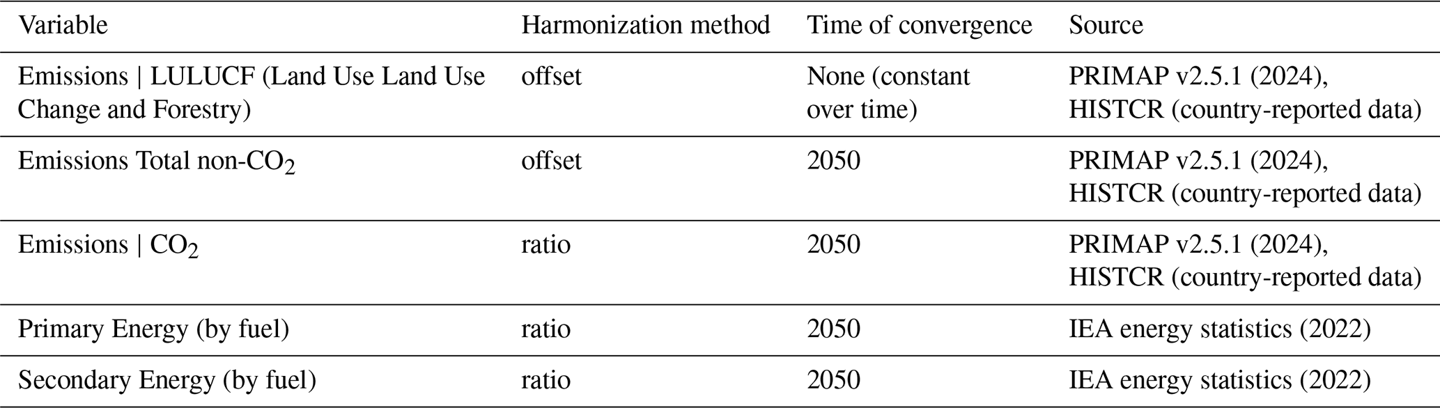
We do not harmonize final energy data with historical data, as the definition of end-use sectors (transportation, industry, buildings) differs across integrated assessment models.

While harmonizing the downscaled results to historical datasets, we create additional “statistical difference” variables, defined as the difference between IAMs results and the sum of (harmonized) country-level data across all regions. This statistical difference normally approaches zero by 2050 to preserve the long-term emissions from IAMs and implications for global warming. However, when downscaling total Kyoto Gases, the statistical difference captures “indirect” LULUCF emissions that are not included by IAMs. Currently, this different method leads to a mismatch of around 5.5 GtCO₂ globally (Grassi et al., 2021). To address this issue, the downscaling algorithm enriches the IAMs results by adding the “indirect” emissions component:

• “Direct” emissions are fully harmonized, so that the sum across countries align with regional IAMs results

• “Indirect” emissions are harmonized to match historical inventories data (using a constant offset over time).

Therefore, on the one hand downscaled results are fully consistent with regional IAMs results when considering “direct” land-use emissions only. On the other hand, they are aligned with national inventories when considering the sum of “direct” and “indirect” land-use emissions.

3 Results

We employ DCSCALE to provide country level downscaled results for the NGFS 2023 project. This paper focuses on the results of four key regions within the MESSAGE model: Sub-Saharan Africa, China, Western Europe, and Pacific OECD. We focus only on four regions as the core objective of this paper is to present the downscaling methodology and to demonstrate its application in the context of the NGFS project with a few examples. We have selected these regions by considering different aspects:

• Number of countries: including the Sub-Saharan Africa region (48 countries) and the China region (only 2 countries)

• Future socio-economic projections across countries: Pacific OECD region (including Japan with ageing population and Australia with increasing population)

• Including both regions from the global North and global South:

  • Western Europe, with strong convergence in policies in some countries (EU27) as well as possible outliers (e.g. Turkey),

  • Sub-Saharan Africa region encompassing low-income countries (e.g. Burundi), upper-middle income countries (such as South Africa and Equatorial Guinea) and high-income countries (Seychelles).

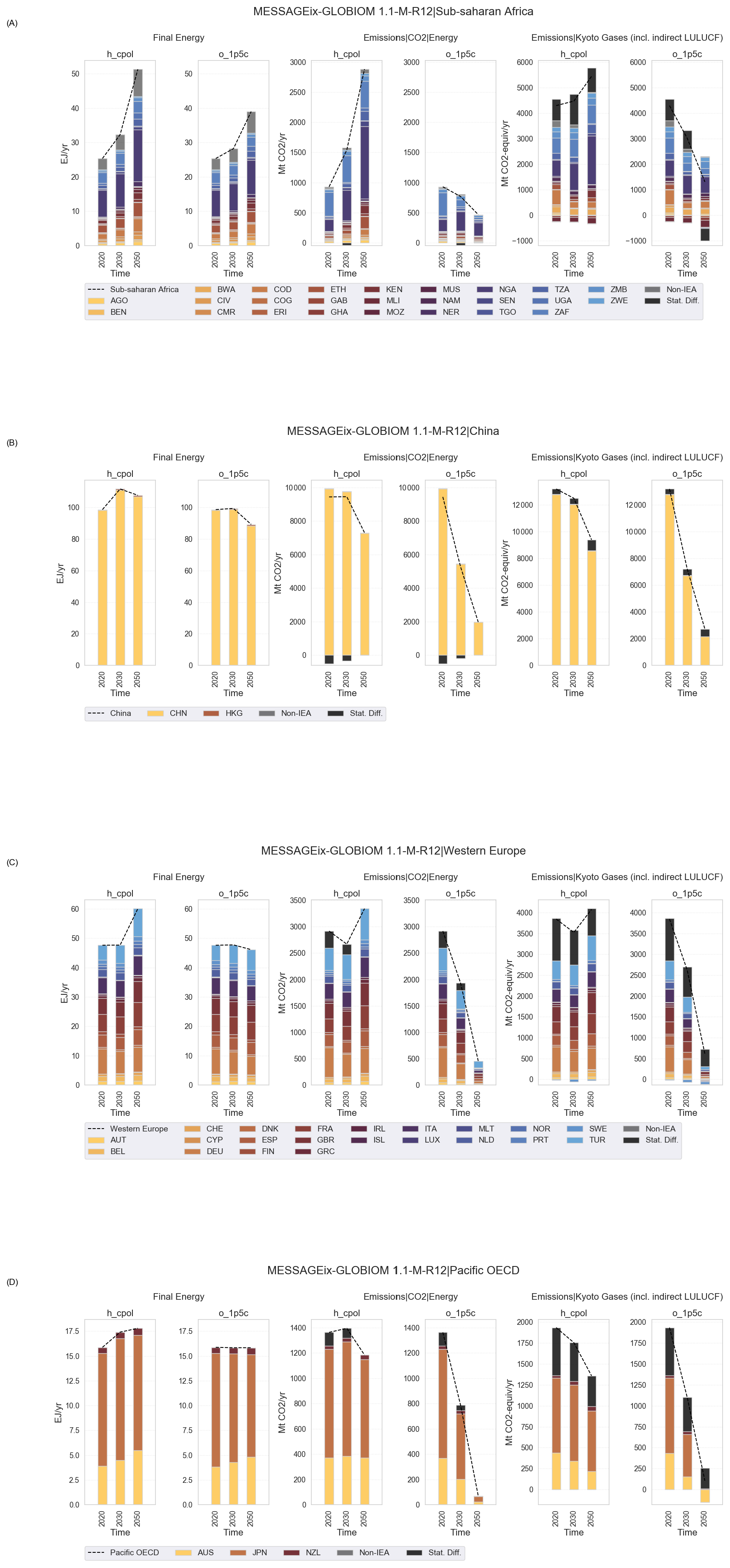
Figure 4 Downscaled results from the Sub-Saharan Africa (a), China (b), Western Europe (c) and Pacific OECD (d) regions of the MESSAGE model, under a Current policy and 1.5 °C scenarios. Selected variables: Final Energy, Energy related CO₂ emissions and Kyoto Gases (including indirect LULUCF).

Figure 4 illustrates the downscaled results in a current policy and a 1.5 °C scenario for selected variables: Final energy, Energy related CO₂ emissions and Kyoto Gases (including indirect land use emissions).

In the Pacific OECD region, energy-related CO₂ emissions show diverse trajectories contingent upon the scenario under scrutiny. In the current policy scenario, regional emissions from energy are projected to peak around 2025 and then gradually decline over time. However, in Japan emissions are expected to decline from 2030 to 2035, primarily due to demographic shifts, such as an aging population. This demographic trend reduces energy demand, contributing to the observed decline in CO₂ emissions from energy. In 1.5 °C scenario, energy-related CO₂ emissions need to peak during the 2020–2030 decade across all countries in the Pacific OECD region, reflecting concerted efforts to limit global warming. Specifically, Japan and Australia are expected to mitigate emissions between 2020 and 2030, with reduction rates of 40 %–45 %. Renewables would need to cover between 21 % and 33 % of total primary energy by 2030 in Japan and Australia respectively, compared to about 10 % observed in 2020. With renewable energy accounting for 35 %, New Zealand has the cleanest energy mix in this region in 2020. For this reason, its emissions are required to decline at a modest 5 % rate between 2020 and 2030.

When downscaling total Kyoto Gases, a statistical difference arises due to the inclusion of indirect Land Use, Land-Use Change, and Forestry (LULUCF) emissions, which are not accounted for by IAMs (Grassi et al., 2021). This different accounting method results in Kyoto Gases emissions in the Pacific OECD region being approximately 250 MtCO₂ lower compared to native IAMs results. Under the 1.5 °C scenario, Kyoto emissions in the Pacific OECD region are projected to fall below zero, especially in Australia. This is mainly due to negative land use emissions outweighing other sources of emissions.

In the Sub-Saharan Africa region, energy consumption is projected to increase over time. Among the countries in this region, Nigeria (NGA) stands out as the largest energy consumer across all scenarios. Growing population and GDP, contribute to increasing energy demand for various purposes, including transportation, electricity generation, and industry. By the year 2050, Nigeria is projected to surpass South Africa as the largest emitter of energy-related CO₂ emissions within the region.

In contrast, energy-related CO₂ emissions in South Africa are expected to remain relatively stable during the 2020–2030 period in the current policy scenario. However, under the 1.5 °C scenario, emissions are projected to decline. This decline is pushed by a significant increase in renewable energy generation (more than doubling compared to 2020), with a fast deployment of wind and solar, leading to phasing out coal-based power plants. Additionally, negative emissions uptake from the land use sector contributes to offsetting non-CO₂ emission sources in the 1.5 °C scenario.

In China (CHN), energy consumption is projected to decline beyond 2035, in both scenarios, with deeper reductions in the 1.5 °C scenario. These results are largely driven by the outcomes derived from the regional data of the MESSAGE model, which encompasses both China and Hong Kong, leaving small margin for uncertainty associated with the downscaling methodology (see sensitivity analysis section). Under the 1.5 °C scenario, both energy-related CO₂ and Kyoto emissions in China need to sharply decline during the 2020–2030 period, followed by a stabilization at or slightly below present-day levels in the subsequent years. By the year 2050, emissions need to be reduced to approximately 2 gigatons of CO₂-equivalent, or even lower for energy-related CO₂ emissions. Similarly, in Hong Kong, both Kyoto and energy-related CO₂ emissions are projected to decrease by 25 % during the 2020–2030 decade and by more than 50 % by 2050. These reductions will be enabled by the gradual phasing out of coal and gas consumption replaced by renewables energy, especially wind.

In the Western European region, energy use will slightly increase under a current policy scenario and stabilize over time in the 1.5 °C scenario. In both scenarios Turkey will overcome Germany as the largest energy consumer and emitter by 2050. This shift is driven by higher GDP growth rates compared to other countries within this region. This finding is reinforced by the hindcasting analysis (see hindcasting section), which reveals that downscaled energy-related CO₂ emissions in Turkey tend to be slightly underestimated in the short term, indicating a potential underestimation of emissions and energy consumption in Turkey. In the Paris Agreement scenario, Germany need to achieve net zero greenhouse gas (GHG) emissions by 2050. Other countries in the region, including France, Italy, Spain, Sweden, and Finland, are projected to achieve net-negative emissions of Kyoto gases, in line with the climate goals outlined in the EU mid-century strategy. However, in other countries outside the EU such as Turkey, GHG emissions are projected to remain above zero by 2050 due to a slower pace of decarbonization in the energy sector compared to other more developed economies in the region.

In the context of the NGFS 2023 project, our algorithm allowed for coupling the IAMs results (downscaled to the country level) with NiGEM (National Institute Global Econometric Model) (Hantzsche et al., 2018), a leading macroeconomic model, used by private sector organizations and policy makers for economic forecasting, stress testing and scenario building. In a similar manner, downscaled results could be used as input for additional analysis. For example, country level models could identify cost effective energy transitions under an exogenous carbon emission trajectory (or carbon budget) in line with the 1.5 °C scenarios from IAMs.

Additional figures for the remaining MESSAGE regions can be found in the Supplement (Sect. S4). The full dataset with the downscaled results across all NGFS models (MESSAGE, GCAM and REMIND) is archived on Zenodo¹.

4 Sensitivity analysis

This section conducts a sensitivity analysis to explore the range of results from key downscaling assumption. A first assumption involves choosing from which region each country should be downscaled. For the NGFS project, we use regional IAMs results available from the lowest level of regional disaggregation. For example, we downscale Australia from the Pacific OECD region of the MESSAGE model. However, in principle Australia could be downscaled from other regions, for example the World or the OECD region. The hindcasting section (see Sect. 5) will assess how the regional mapping affects the downscaled results, by checking the performance of the downscaling algorithm against historical data, using different regional resolutions.

Beside the regional mapping, this section focuses on other downscaling assumptions that will affect the outcome of specific variables. Table 9 summarizes how exogenous drivers (such as country-level socioeconomic projections from different SSPs) as well as other downscaling assumptions can lead to different country-level projections.

Table 9 Uncertainty levers associated to exogenous data and downscaling parameters.

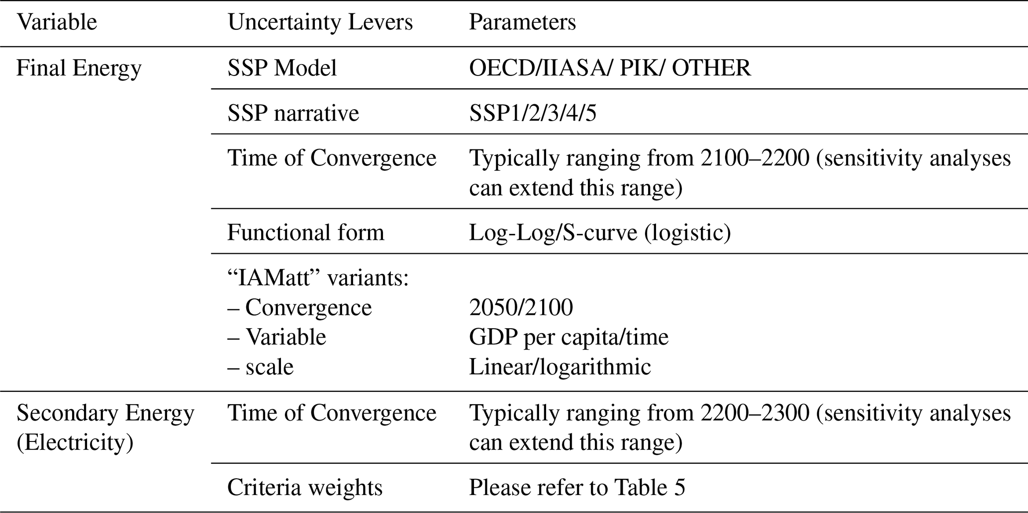
Data and downscaling assumptions have a direct effect on the downscaled results leading to an uncertainty range. For example, exogenous GDP and population projections from SSPs storylines (and their underlying SSP model) have an influence on the evolution of downscaled final energy variables. For the NGFS 2023 project we rely on ad-hoc socioeconomic projections that consider the COVID-19 impact on the economy and expected recovery, followed by a growth in line with the SSP2 (middle of the road) storyline. However, this sensitivity section will focus only on the direct effects arising from key downscaling assumptions.

For final energy, variables these assumptions include the type of model used in the historical trend regression (log-log or s-curve), the time of convergence “tc” as well as alternative “IAMatt” variants. The impact of these assumptions is assessed in the Sect. 4.1

Secondary energy electricity variables are affected by the time of convergence “tc” as well as the criteria weights used in the “NAT” path (see Sect. 4.2).

4.1 Final Energy

Final energy results are affected by assumptions about (1) the functional form used in the regression, (2) the convergence assumptions towards the default “IAMatt” path, and (3) the alternative “IAMatt” variants.

4.1.1 Uncertainty due to the functional form

Assumptions about the functional form determine how energy demand evolves in relation to GDP per capita. Historical trends at the country level suggest that the overall energy intensity (final energy divided by GDP) declines with increasing GDP per capita. Future energy intensities can be extrapolated by using a log-log function or a logistic curve. The linearized log-log function is easy to estimate and implement. It nicely replicates historical trends at the country level, while keeping the energy intensity results non-negative. Conversely, a logistic function is usually better suited when historical or future developments are characterized by non–linear patterns. For these reasons, they are widely used when modelling the penetration of technologies in each market, or the share of an energy carrier in the overall energy consumption.

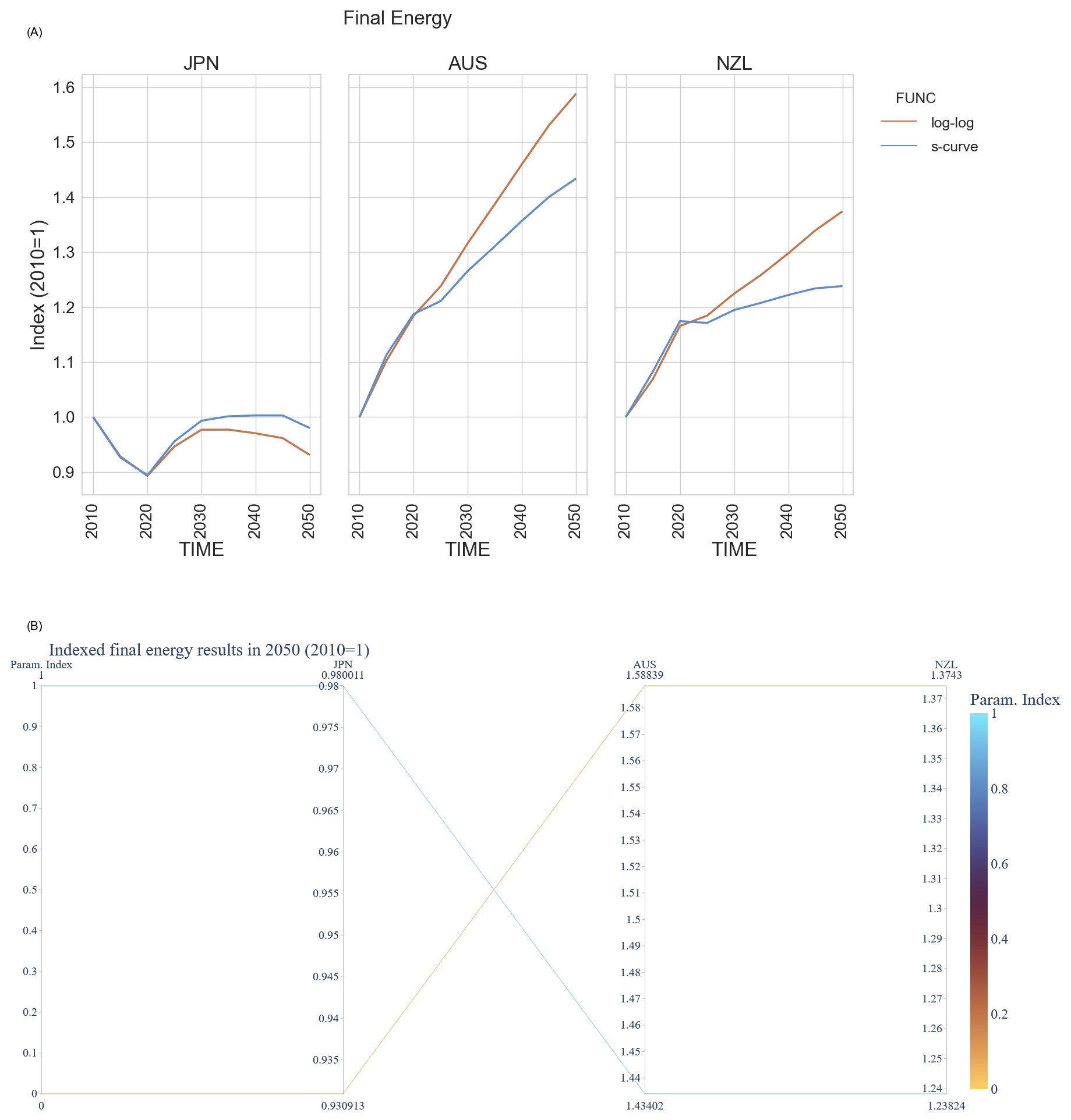
Figure 5 Uncertainty range due to functional forms: log-log (orange) and s-shape (blue). Panel (A) shows downscaled final energy results for Australia New Zealand and Japan under a current policy scenario. Panel (B) shows the results for 2050 using a parallel coordinate plot (in total two lines are shown labelled as 0 and 1 (corresponding to the log-log and logistic curve respectively).

To employ a logistic functional form, we modify Eq. (6) as shown in Eq. (39):

$$\begin{array}{}\text{(39)}& I_{t,c}=\left\{\begin{array}{l}\frac{\mathrm{L}}{\mathrm{1}+e^{-k\left(x_{t,R}-x_{\mathrm{0},R}\right)}}\text{if\hspace{0.17em} path}=\mathrm{IAMatt}\\ \frac{{\mathrm{L}}_c}{\mathrm{1}+e^{-k_c\left(x_{t,c}-x_{\mathrm{0},c}\right)}}\text{if\hspace{0.17em} path}=\mathrm{NAT}\end{array}\right.\end{array}$$

L denotes the carrying capacity (upper bound of the logistic curve), x is GDP per capita (with x₀ representing the inflection point of the curve) and k denotes the steepness of the logistic curve. In this section we compare the final energy results arising from energy intensity modelled with a log-log functional vs a logistic function, as shown in Fig. 5.

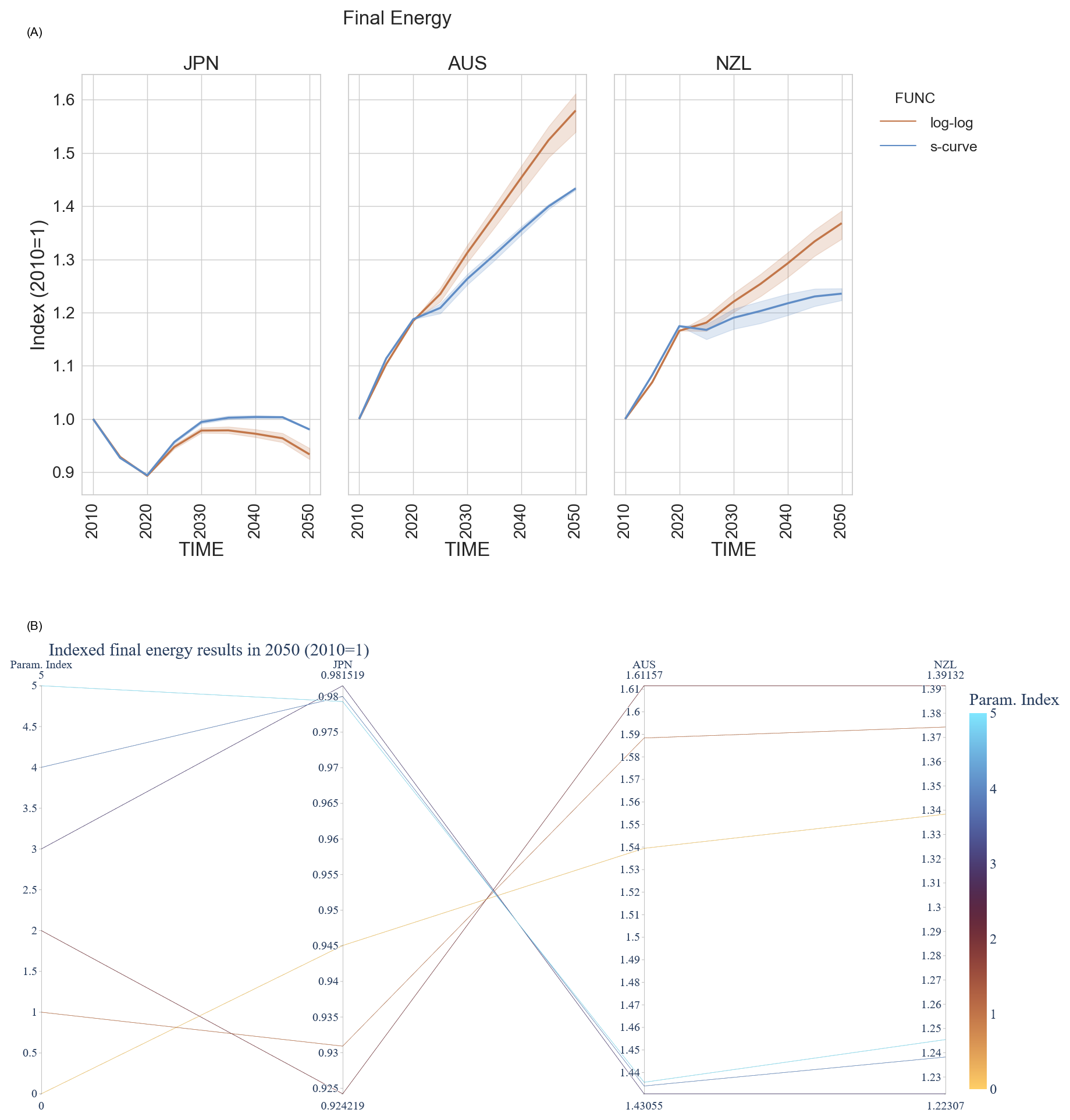
Figure 6 Uncertainty range including functional forms (by color) and convergence range (shade area). Panel (A) shows downscaled final energy results for Australia New Zealand and Japan under a current policy scenario. Panel (B) shows the results for 2050 using a parallel coordinate plot (in total 6 lines are shown: two variants for the functional form and three variants for the convergence assumptions). Detailed information about the parametrization index is provided in the Supplement.

4.1.2 Uncertainty due to the convergence assumptions

Assumptions about the convergence form the “NAT” path (mostly driven by historical trends) to the “IAMatt” path (with trends derived from regional IAMs scenarios) leads to a range of uncertainty. A slow convergence will preserve the historical trends for longer time periods, whereas a fast convergence will rely more on regional IAM information. The uncertainty is larger when differences between the “NAT” and the “IAMatt” paths are more pronounced.

In our default parametrization” we use an “IAMatt” path that is entirely informed by future IAMs scenarios and country level socioeconomic projections, without considering the current energy consumptions across countries. For the sensitivity analysis, we develop alternative “IAMatt” variants, which are also informed by historical country level data. The next sub-section assesses the uncertainty range arising from these new IAMatt variants.

4.1.3 Uncertainty due to “IAMatt” variants

In this section we provide alternative “IAMatt” variants that consider historical final energy data at the base year in each country. These variants can provide a wider range of results, which are particularly useful in case of disruptive scenarios, where the need for deep energy reductions should be balanced with historical data considerations. Such scenarios may be characterized by low energy demand projections and stagnating (or declining) GDP per capita.

To achieve this goal, we interpolate the historical data in 2010 (t0) to the values observed in the default “IAMatt” in “tc*” (e.g. 2050) as shown in Eqs. (40) and (41).

$$\begin{array}{}\text{(40)}& {\displaystyle }{\mathrm{IAMatt}}_{t,c,e,s,tc}^{\ast }={\mathrm{\varnothing }}_{t,\mathrm{tc}}^{\ast }{\mathrm{histdata}}_{t\mathrm{0},c,e,s}+\left(\mathrm{1}-{\mathrm{\varnothing }}_{t,\mathrm{tc}}^{\ast }\right){\mathrm{IAMatt}}_{t,c,e,s}\text{(41)}& {\displaystyle }{\mathrm{\varnothing }}_{t,\mathrm{tc}}^{\ast }=max\left\{\mathrm{0},{\displaystyle \frac{{\mathit{\gamma }}_t-{\mathit{\gamma }}_{t{c}^{\ast }}}{{\mathit{\gamma }}_{t\mathrm{0}}-{\mathit{\gamma }}_{t{c}^{\ast }}}}\right\}\forall t<t{c}^{\ast }\mathrm{else}\mathrm{0}\text{(42)}& {\displaystyle }\mathit{\gamma }=\log \left(\mathrm{\Gamma }\right)\text{if\hspace{0.17em} scale}=\log \mathrm{else}\mathrm{\Gamma }\end{array}$$

This function can be applied over a generic variable Γ such as time or regional GDP per capita, using a linear or a log scale, as shown in Eq. (42).

Therefore, three dimensions affect the alternative “IAMatt*” variants:

• the time of convergence tc* (e.g. 2050 or 2100)

• the scale (linear or log)

• the variable (e.g. regional GDP per capita or time) used to calculate the weights ∅

Please note that with a time of convergence tc* equal to 2010, we obtain the default “IAMatt” path (as the convergence to the default IAMatt path starts immediately). Figure 7 shows the full uncertainty range when adding a range of IAMatt variants.

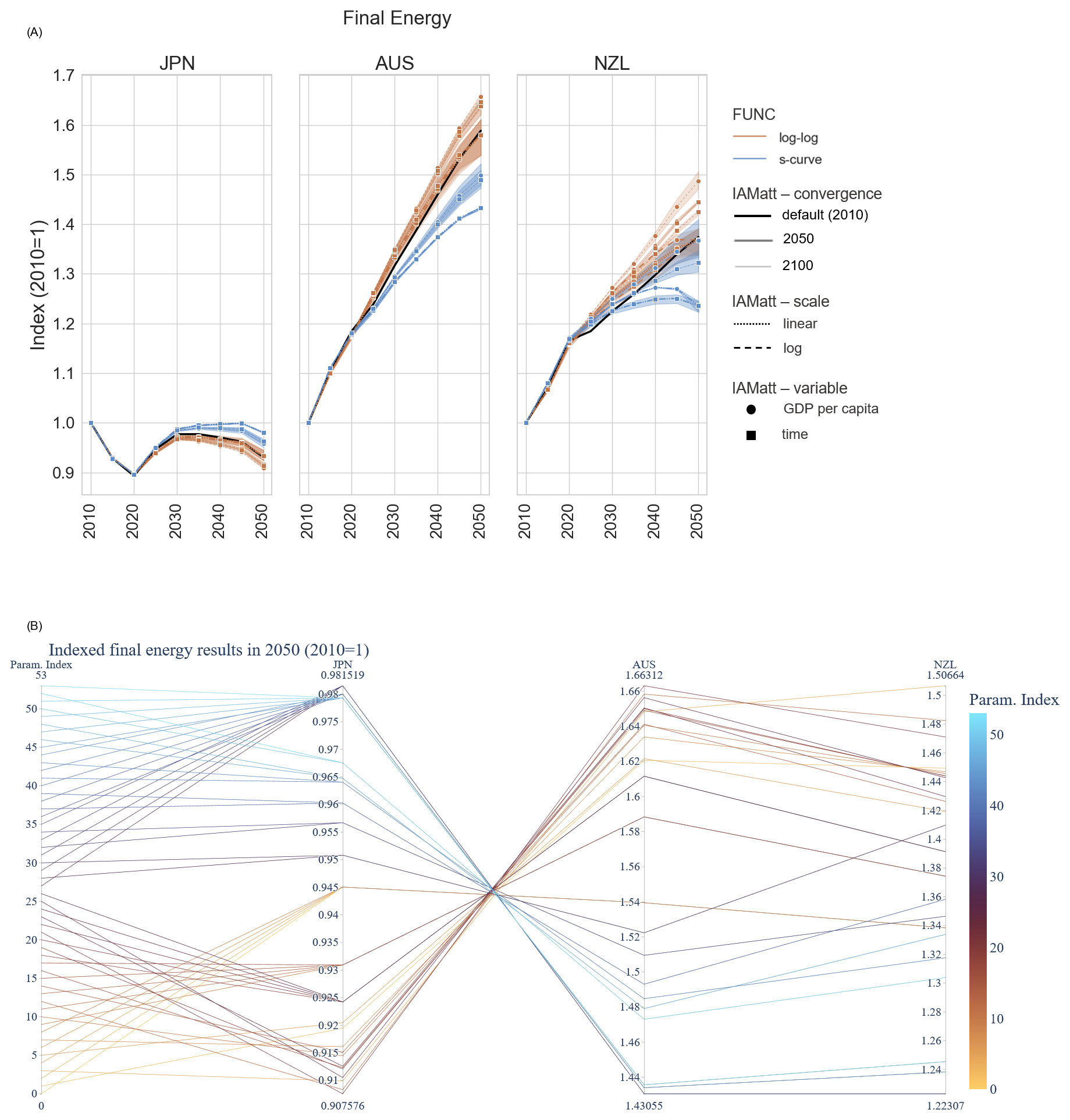
Figure 7 Full uncertainty range including functional forms (by colour), convergence (shade area) and IAMatt variants (line style). Panel (A) shows downscaled final energy results for Australia New Zealand and Japan under a current policy scenario. The solid (thick) black line shows the default IAMatt path (time of convergence =2010). Thinner lines indicate a later time of convergence (“IAMatt” variants). Circles indicate an interpolation over regional GDP per capita, whereas square symbols time. Dotted lines indicate a connection using a linear scale, whereas dashed lines indicate a log scale. Panel (B) shows the results for 2050 using a parallel coordinate plot. Line numbers are sorted to match the colour code of the functional forms: log-log (orange) and s-shape (blue). Detailed information about the parametrization index is provided in the Supplement.

The uncertainty range is lower for Japan, as it is the dominant country in the Pacific OECD region of the MESSAGE model. As a result, a higher energy consumption in Japan is associated to lower demand in New Zealand and Australia. This occurs because DSCALE ensures that results align with regional IAMs data, maintaining a consistent sum across all countries. This constraint reduces uncertainty and enhances the robustness of the results for the largest countries in the region.

To conclude, by varying the downscaling assumptions, DSCALE provides a range of projections at the country level, all of them in line with regional IAM scenarios. For some use cases, like the NGFS project, we provide a single default path for each country (without a range of uncertainty), using an “IAMatt” path completely disconnected to historical data. This simple assumption is advisable when future IAMs scenarios/storylines envision increasing GDP per capita over time. However, in case of particularly disruptive scenarios, characterized by sharp decline in energy demand and declining (or stagnating) GDP per capita, we recommend using alternative “IAMatt” variants that consider observed historical data. The next section will show how different energy demand projection affect the electricity generation in each country.

4.2 Electricity

This section performs a sensitivity analysis on the secondary energy electricity results. The electricity mix is affected by the assumptions on criteria weights, the previously downscaled electricity demand, and the convergence assumptions. The criteria weights influence only the “NAT” path, whereas electricity demand and the timing of convergence affect the “composite” path. This section explores the uncertainty range at different stages in the downscaling process.

4.2.1 Uncertainty in the NAT path (criteria weights)

Criteria weights, affect the secondary energy electricity results in the “NAT” path. To assess how these assumptions change the electricity results, we run DSCALE using a range of randomly generated weights, (instead of the default criteria outlined in Table 5). This sensitivity analysis focuses on Australia and New Zealand, both downscaled from the Pacific OECD region of MESSAGE, under a current policy scenario. The results of the analysis depend on the number (n) of randomly generated criteria weights used in the simulation. In order to determine the number of random criteria, we run two set of simulations (A and B) with a number of random criteria weights n. The randomly generated criteria are completely independent across the two simulations. As the number of randomly generated criteria increases, we expect the distribution of the results from simulations A and B to converge. Therefore, we keep on running the simulations until the results from the two simulations will converge to a similar distribution, usually with n=500.

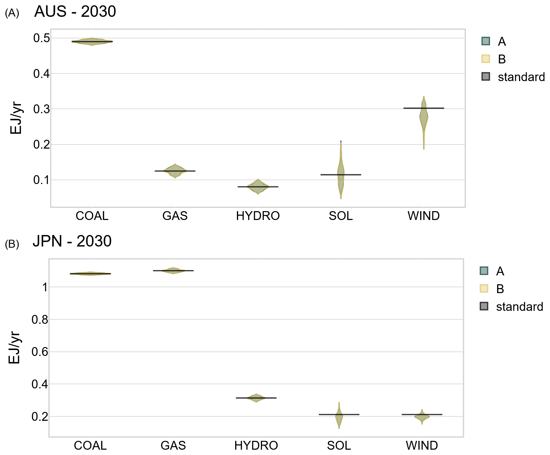
Figure 8 Electricity generation by fuel (distribution) in Australia (AUS) and Japan (JPN) in 2050, downscaled from the MESSAGE current policy scenario. We have run two simulations (A, B), each of them with completely independent (n=500) randomly generated electricity criteria. The distribution of the results is depicted in light blue (A) and yellow (B) from the two sets of randomly generated criteria. The black line represents the “standard” criteria used for the NGFS 2023 project. The graph does not show results for nuclear, biomass, geothermal and oil as they are equal (or close) to zero at the regional level in 2030, leaving no room for an uncertainty range.

Figure 8 shows that with n=500 randomly generated criteria, the two simulations (A and B) tend to convergence to the same distribution. For big countries within a region – such as Japan – the uncertainty is lower, as the sum of all country-level results need to match the regional IAMs results.

Regarding the distribution across fuels, the uncertainty is higher for solar and wind, where the allocation across countries varies a lot depending on the criteria chosen (historical data, stranded assets, governance, and cost curves).

There is virtually no uncertainty for oil-based power plants as well as nuclear technologies, as they will be phased out at the regional level, leaving no uncertainty associated to the downscaling method. For this reason, these fuels were omitted from the graph (for completeness, they can be found in the Supplement).

There is uncertainty associated to fossil-fuel power plants such as gas and coal, which are affected by currently installed (and planned) capacities as well as the age of the fleet. Hydropower plants are affected by how we change weights associated to historical data and resources availability at a given cost.

It is important to note these results refer to the “NAT” path, before the structure adjustments (see Sect. 2.3) aiming at minimizing the gap between electricity demand and supply. The next sub-section will show the results from the “composite” path (after electricity trade minimization), where “NAT” and “IAMatt” paths are merged depending on the time of convergence. In this manner, we disentangle the uncertainty arising from electricity demand, the criteria weights and convergence assumptions.

4.2.2 Uncertainty in the “composite” path

The uncertainty in the “composite” path arises from three factors: (1) criteria weights, (2) electricity demand and (3) convergence assumptions. This section assesses how the uncertainty from these three components leads to a range of results.

For the “composite” path, we do not apply the entire set of 1000 criteria (500 for each of the two distributions A and B), as was done in the previous section for the “NAT” path. Instead, we focus on selecting only the criteria associated with the median, minimum, and maximum outcomes for each fuel type and across all countries. This reduces the number of criteria weights to 37 (instead of 1000), while still capturing the full range of results observed for each fuel in all countries. Figure 9 illustrates the distribution of electricity generation by fuel type in 2050 for Australia and Japan under a current policy scenario.

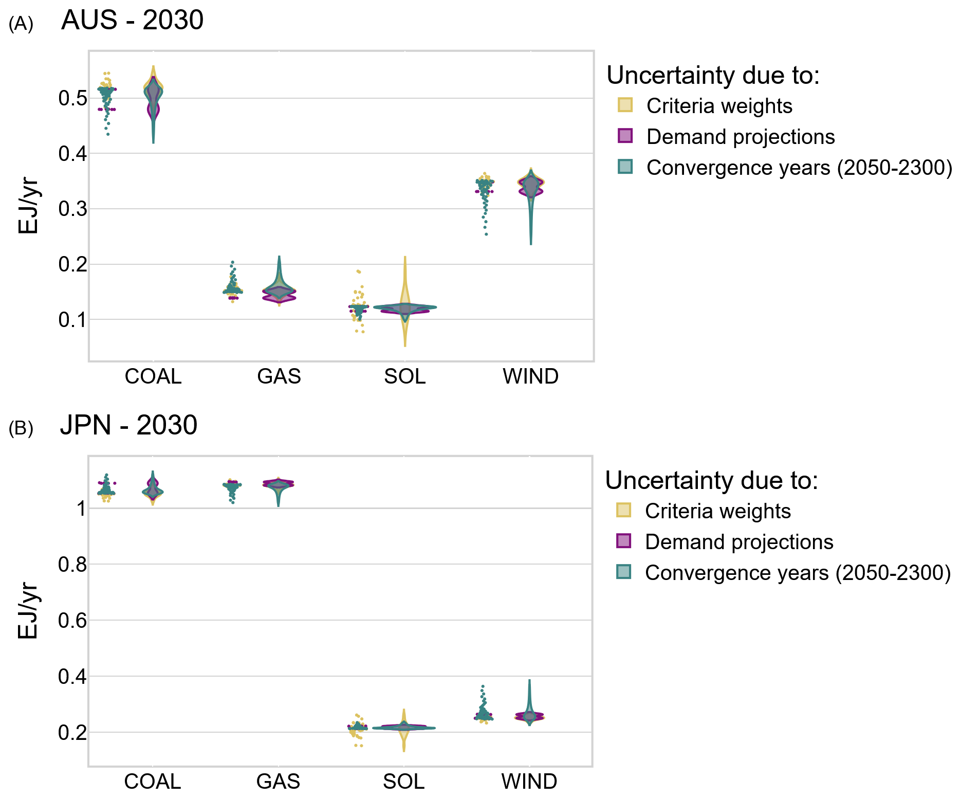
Figure 9 Uncertainty range in the electricity mix in Australia (AUS) and Japan (JPN) in 2030, downscaled from the MESSAGE current policy scenario, under the “composite” path. The graph shows the uncertainty arising from different components including: (i) criteria weights (n=37), (ii) “demand” projections (n=18), (iii) “convergence” (n=51).

Figure 9 shows the distribution of electricity generation in the “composite” path by fuel in 2030, downscaled from the current policy scenario of MESSAGE. The graph does not show the results for biomass, oil, nuclear, geothermal and hydro energy as these values are small at the regional, leading to a minimal range of uncertainty. For completeness, the sensitivity analysis for these fuels is shown in the Supplement.

The graph shows the uncertainty range in the “composite” path arising from criteria weights (gold), final energy demand projections (purple) and convergence years (light blue). Regarding the criteria weights, it should be noted that unlike the “NAT” path, the “composite” path includes an additional constraint aimed at aligning electricity supply with domestic demand, while ensuring that the sum across countries matches the regional IAM results (as explained in Sect. 2.3 on structural adjustments). This balance between these constraints results in a more evenly distributed range of uncertainty across fuels. Therefore, final energy electricity projections have an impact on the electricity mix because the algorithm scales up/down all fuels to meet the demand. This also leads to a multimodal distribution associated the demand projections, with two peaks corresponding to each functional form (log-log and s-curve). Finally, the light blue colours show how the timing of convergence affects electricity generation.

Interestingly, the results for solar in Australia are mostly driven by criteria weights. More details are available in the Supplement, showing how different weight for each criteria affect the results. The convergence assumptions also have a strong influence on the electricity mix, with a skewed distribution towards late timing of convergence.

To conclude, in the “composite” path, the range of uncertainty is more evenly distributed across the different fuels compared to the “NAT” path, and the uncertainty range is generally lower for bigger countries (such as Japan).

5 Hindcasting analysis

This section conducts a hindcasting analysis by applying the downscaling tool to the historical time frame from 2010 to 2020, instead of regional IAMs results. We assess the performance of the algorithm by comparing the results with the observed historical data as well as a simpler (proportional) downscaling method. Finally, we assess how different regional mapping affect the downscaling results. Given the high volatility observed in historical land use emissions, our analysis focuses on energy-related CO₂ emissions.

Historical data are accessible for nearly all countries globally. This allows us to calculate regions by summing up the data for selected countries. Consequently, for the hindcasting analysis, we theoretically have the flexibility to downscale any country from any region. For instance, Turkey could be downscaled from various regional configurations containing Turkey and additional countries, leading to many regional combinations. To streamline the hindcasting analysis, we focus on three regional configurations based on country mappings from the MESSAGE (Huppman et al., 2019), GCAM (Calvin et al., 2019), and REMIND (Luderer et al., 2022) models. These configurations are applied to a selected group of countries, as outlined in table 10 (countries are identified using ISO-3 codes).

Table 10 Selected countries and corresponding regional mapping, based on the IAMs MESSAGE, REMIND and MESSAGE. The selected country (ISO code, shown in the first column of the table) within the list of countries in a given region are displayed in bold font.

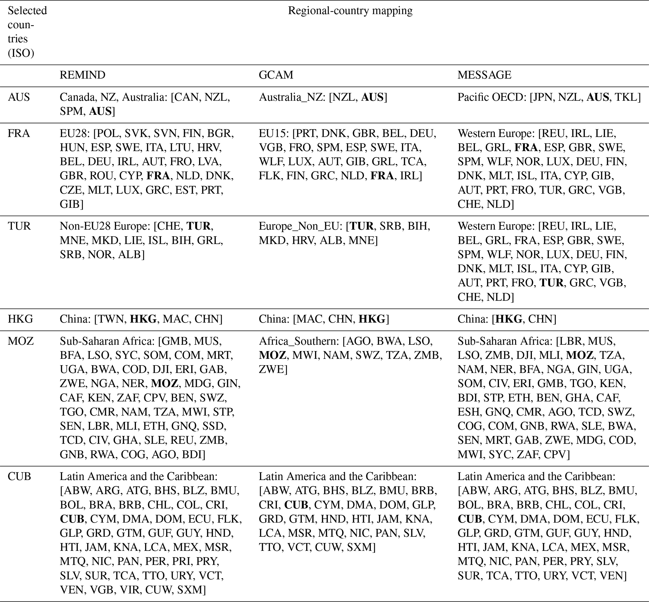
For instance, we downscale Turkey (TUR) from the following regions:

1. the “Europe_Non_EU” (GCAM regional mapping),

2. “Western Europe” (MESSAGE regional mapping)

3. “Non-EU28 Europe” (REMIND regional mapping).

Hence, in this section, references to “MESSAGE”, “GCAM”, and “REMIND” denote distinct regional mappings (i.e., the list of countries within a region), while the regional data are directly sourced from historical data². The aim of this section is to illustrate how different regional mappings may influence the downscaling results, given that the regional data align precisely with the historical data. At the same time, we compare the results with a simpler proportional downscaling method, which preserves the share of countries within a region as observed at the base year. This simple approach is suitable for short time frames, for example up to 10 years. However, in the long run this approach may underestimate emissions in developing countries, therefore leading to higher emissions in mature economies, like the OECD countries (van Vuuren et al., 2007).

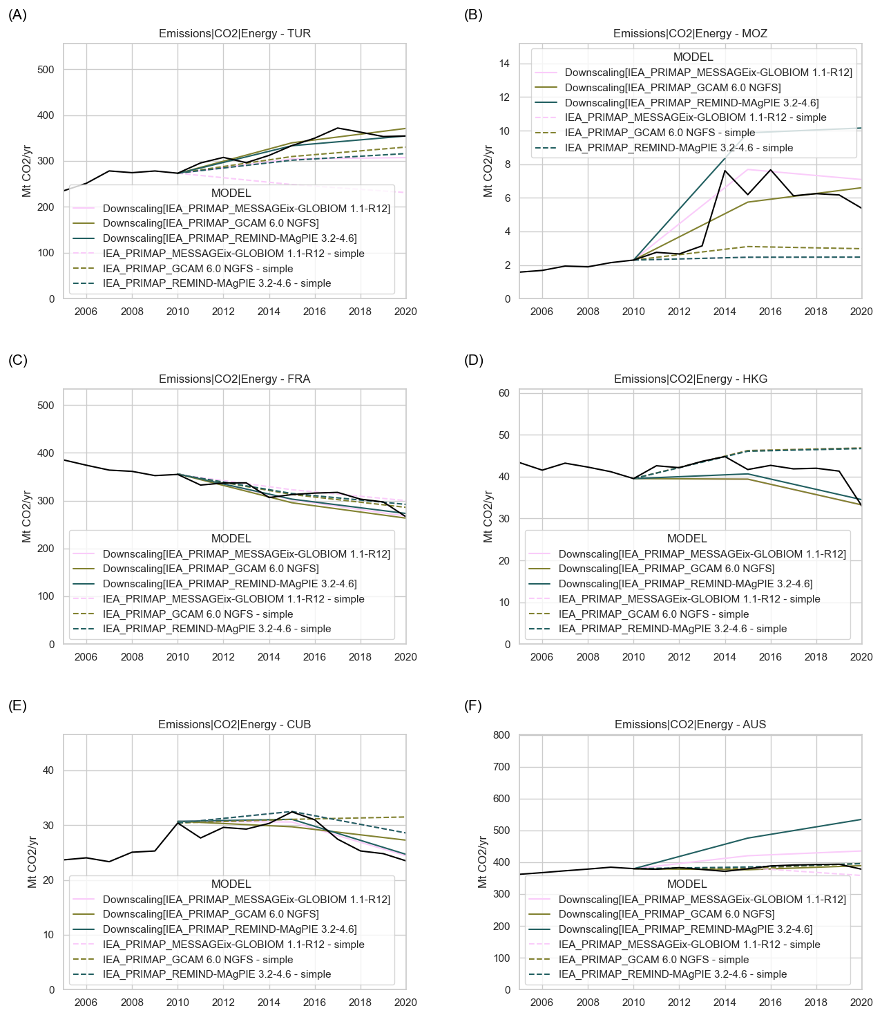
Figure 10 Hindcasting results for energy-related CO₂ emissions (from 2010–2020) for selected countries. Coloured solid lines show the downscaled results using three different regional mappings, based on REMIND (light blue), GCAM (green) and MESSAGE (pink). Black lines indicate data from the PRIMAP dataset. For comparison purposes, dash lines show the downscaled results using a simple (proportional) downscaling method.

Figure 10 shows the hindcasting analysis for the period 2010–2020 comparing the results from the downscaling algorithm (solid lines) with a simple downscaling method (dashed lines) and observed energy-related CO₂ emissions from PRIMAP (black solid lines). Different colours (based on the scientific colour map “batlowS” (Crameri, 2018, 2023; Crameri et al., 2020)) represent the regional mappings, from MESSAGE (pink), GCAM (green) and REMIND (light blue). Overall, we find a good level of agreement between the downscaled results and observed historical data, with enhanced performance linked to the use of finer regional resolutions. For instance, results for Turkey (TUR) show that the hindcasting performance enhances when using the regional mapping of GCAM (“Europe_Non_EU”), compared to the MESSAGE mapping (“Western European” region). The downscaling algorithm replicates well the observed historical data from PRIMAP (black solid line), better than a simpler (proportional) downscaling method. This is generally the case for fast growing economies within a region.

An interesting case is Mozambique (MOZ), which experienced an average GDP growth rate of 7.2 % between 2010 and 2015, followed by a drop to an average of 2.4 % from 2015 to 2020. The downscaling algorithm considers these growth rates, and for this reason outperforms simple proportional downscaling methods that fail to account for such GDP dynamics. The results also reveal significant uncertainty stemming from different regional resolutions. Therefore, we recommend using various IAM outputs where possible and conducting sensitivity analyses to ensure robust insights and well-informed policy recommendations.

For developed economies like France (FRA), the downscaled results mirror quite well the observed data, with low uncertainty across all different regional mappings (EU15, EU28 and Western Europe), and with a better performance than the proportional method.

Another noteworthy example is the Latin America Region from MESSAGE, GCAM and REMIND. While the three regional mappings share the same region name, their definitions vary. For example, Brazil, Argentina, and Venezuela are part of the Latin American region of the MESSAGE and REMIND model, but they are not included in the GCAM model. Therefore, the regional resolution of the Latin America region can largely differ depending on the model chosen. Figure 10 shows the hindcasting results for Cuba, replicating relatively well the historical data.

The results for energy-related CO₂ emissions are promising, even when small countries like Hong Kong (HKG) are downscaled from larger regions, such as China. In this case, both the downscaling algorithm and simpler methods perform reasonably well in replicating observed data, with only minor differences between the two approaches.

However, there are instances where simpler methods may outperform the downscaling algorithm, particularly when a country deviates from the historical trends and is downscaled from a relatively large region. For example, under the REMIND regional mapping Australia shows higher emissions due to an overestimation of energy and electricity demand heavily reliant on coal-fired power plants. These deviations tend to diminish when finer regional resolutions are used (e.g., the “Australia_NZ” region of GCAM), as the sum across all countries needs to line up with the regional results.

6 Discussion

In this study we downscale 12 MESSAGE regions to individual countries, to provide a consistent assessment of national pathways in line with the NGFS scenarios. We rely on the regional-country mapping definitions as provided by the IAM teams, which is based on the UN definition of countries (with associated ISO-3 codes). In addition, we rely on future socioeconomic projections from the SSPs storylines (Bauer et al., 2016, 2017; Fricko et al., 2017; Riahi et al., 2017a, b), and on historical data from the International Energy Agency (IEA, 2022), which are not always available for all countries.

It is also important to note that there are methodological challenges in translating idealized pathways (based on cost minimization or welfare maximization approaches) from global regions into plausible country level trajectories. DSCALE addresses this issue by combining historical trends with IAMs scenarios in a way that preserves realism, while remaining consistent with future regional pathways. To this end, in our default assumption, the energy intensity projections are modelled as a function of GDP per capita where steepest structural changes are assigned to higher-income countries, that are better equipped to lead the transition. Therefore, SSPs storylines play an important role when projecting final energy demand. The NGFS project relies on income per capita projections from the SSP2 (Middle of the road) storyline, where GDP per capita is generally assumed to grow across all countries. However, other SSP narratives like SSP3 (Fujimori et al., 2017b) or SSP4 (Calvin et al., 2017), may envision stagnation or decline in income per capita projections, hence affecting the pace of energy system transformation in some countries.

The relationship between energy intensity and GDP per capita has been widely assessed in the literature (Energy Inefficiency in the US Economy, 2024; Energy Primer, 2021; Nakicenovic et al., 1990, 1998; Nakićenović et al., 1993). We apply similar relationships when downscaling final energy across different sectors (industry, transportation and residential & commercial) and energy carriers (electricity, liquids, solids, gases). However, these relationships may weaken as we go further with the disaggregation process, leading to higher uncertainty in future projections. To mitigate this issue, DSCALE ensures a strict order of disaggregation:

• A.

  Total Final energy demand is downscaled first to serve as a constraint for energy carriers (e.g. electricity use cannot exceed total energy demand)

• B.

  Energy carriers (e.g. electricity) are downscaled to serve as constraints for sectors

• C.

  Final allocation to sectors, where the uncertainty is higher (e.g. electricity used in Industry), is bound by previous steps

This layered process, combined with regional constraints from IAMs (sum of country level results should align with regional data), limits the uncertainty range. Nonetheless, projections for highly disaggregated sectors remain more uncertain, and future work may consider using machine learning techniques to enhance robustness. However, the use of such methods may hinder the interpretability and transparency of the results.

Regarding national policies, DSCALE optionally integrates targets from NDCs (Nationally Determined Contributions) and LTS (Long Term Strategies). In this context, it should be noted that some countries express their NDCs targets as range, depending on the level of international climate finance. Due the ongoing stalemate in negotiations regarding finance, the NGFS project considers only unconditional NDC targets, and the DSCALE tool adopts the same approach.

Additionally, some countries specify their targets as a percentage reduction below a BAU (Business as Usual) scenario. In this context (Rogelj et al., 2017) emphasizes that the primary source of the uncertainty in the NDCs emissions range stems from the future socioeconomic assumptions. Under the NGFS project we use a consistent set of GDP and population projections across all countries, based on the SSP2 (Middle of the Road) storyline. This approach substantially reduces potential inconsistencies in the interpretation of NDCs targets.

This “national policy” feature enhances the realism of the downscaled results. However, the current version of DSCALE only applies economy-wide targets consistent with the input assumptions of the MESSAGE model, while disregarding sectorial targets. Therefore, the overall national targets are consistent in both DSCALE and MESSAGE, although the sectorial targets may not be fully aligned. This is a clear area for improvement that we will address in future work.

DSCALE operates under the assumption that countries can align emissions with their own NDC and LTS targets by increasing the use of BECCS (biomass with CCS), up to a maximum of 50 % of the national emissions gap. It is important to note that DSCALE will not increase the overall amount of BECCS, as results must be aligned to match regional IAMs results. DSCALE can only allocate the regional amount of BECCS across all countries within that region This means that if BECCS is not available at the regional level in a given time period (e.g. 2030), it will not be allocated to any country, regardless of their emission gap. Moreover, DSCALE will maintain the same level of biomass that was initially allocated to each country (before the “national policy” adjustment): the only parameter that can vary is the percentage of biomass combined with CCS. This adjustment of BECCS is more relevant for countries meeting their net-zero targets and play a very limited role for meeting the NDC targets. A comparison of MESSAGE scenarios against official national projections from (Smith et al., 2025), reveals that downscaled BECCS results are generally lower than the level anticipated by governments by 2050. This comparison in available in the Sect. S5. In conclusion, the amount of BECCS (biomass with CCS) cannot exceed the biomass already in use within each country, and the total BECCS collectively employed in all countries must align with regional IAMs results. These constraints effectively limit the use of BECCS in 2030 and ensure that the results remain plausible in the long term, including by mid-century.

In the NGFS project, negative emissions can be achieved only by using BECCS or via the land use sector. Additional CDR (Carbon Dioxide Removal) technologies (such as enhanced weathering, direct air capture etc.) are not considered by the NGFS scenarios nor by DSCALE.

Regarding land use emissions, different accounting schemes may be used. IAMs usually report only direct land use emissions, while national inventories normally report the sum of both direct and indirect emissions, leading to a global mismatch of about 5.5 GtCO₂ (Gidden et al., 2023; Grassi et al., 2021). To tackle this issue, we enrich the IAMs scenario data by providing downscaled land use emissions results that include both direct and indirect land use emissions. On the one hand, direct land use emissions are fully consistent with regional IAMs results, as their sum across countries matches the regional data. On the other hand, we add indirect land use emissions, which are not reported by IAMs (but that are included in national inventories). Projections of indirect land use emissions are affected by climate variables, including temperature and CO₂ concentration (Grassi et al., 2021) and therefore will vary across different NGFS scenarios. By using this approach, DSCALE provides national pathways that are consistent with IAMs scenarios (for the direct land use emissions component) and that are also harmonized with national inventories (by adding the indirect land use emissions component, not considered by IAMs).

Some parameters within DSCALE are currently set based on expert judgment. These include the default weights used to allocate electricity generation by fuel type, as well as assumptions regarding the time of convergence “tc”. Future work could focus on estimating these parameters empirically, through hindcasting analyses designed to maximize the overlap with observed historical data. However, these optimal configurations may vary based on the regional-country mapping used (hence across different models).

IAMs often provide results for various sets of regions. For instance, they usually provide aggregated results for the so-called “R5 regions”, which include OECD, Asia, Middle East and Africa, Latin America and Reforming Economies. At the same time, they offer more disaggregated “native” regions such as Western Europe, China, Sub-Saharan Africa, and Pacific OCED, in the case of MESSAGE. In this context, a country like Germany belongs to the “R5 OECD” region as well as the “Western Europe” region. In this context, we recommend downscaling the results from the more disaggregated (native) regions, such as “Western Europe”, to ensure consistency with the IAMs results. Moreover, it is important to note that there are different versions of IAMs and some of them can provide results for a handful of individual countries. In this case, we advise using IAMs results for these individual countries directly.

Finally, downscaled results represent a first order translation of IAM scenarios at the country level. These results are derived from top-down IAMs scenarios to evaluate the implications of global scenarios for national pathways. Future efforts may focus on integrating downscaled IAM results with bottom-up models, to analyse outcomes at a finer spatial scale (sub-regions), temporal scale (yearly, monthly, daily, hourly data), finer technological resolutions (e.g, different types of wind turbines, solar PV technologies), including impacts on air quality and on jobs. This would enable a better assessment of the implications of climate change scenarios at the national scale, including potential co-benefits of mitigation strategies.

7 Conclusions

We have introduced a novel algorithm designed to downscale regional Integrated Assessment Models (IAMs) results to the country level, using two main sources of data:

1. country level data, mainly used in the short-term.

2. regional IAMs scenario results, mainly used in the long term.

We complement these data with GDP and population projections at the country level, based on the SSP storylines, hence deriving two paths: a “NAT” path based on country level data, and an “IAMatt” path based on regional IAM scenarios. By merging these two paths using a time of convergence, we derive our final “composite” path.

This paper focuses on the results of the MESSAGE model from the Pacific OECD, Western Europe, China and Sub-Saharan Africa regions under a current policy and 1.5 °C compatible scenarios. Results show how socioeconomic projections influence energy demand dynamics across countries. Notably, declining population in Japan leads to shrinking energy consumption over time, while Australia and New Zealand continue to experience growth. In the Sub-Saharan region, energy related emissions are expected to almost triple under a current policy scenario during the 2010–2050 period, whereas in the 1.5 °C scenario emissions need to halve by mid-century.

Results from the Western European region show that many EU27 countries need to achieve net zero GHG emissions by 2050, including Germany, France, Italy, Spain as well as smaller countries such Finland and Sweden.

The sensitivity analysis shows how different downscaling assumptions lead to a range of results. The timing of convergence affects final, secondary and primary energy variables (and associated emissions), whereas other assumptions are specific for each variable. For the final energy projections, these assumptions include the functional form (type of model) used to estimate future energy demand (either a log-log or an s-curve) and other alternative assumptions related to the “IAMatt” path. In the electricity sector, additional factors include the weighting of historical data, governance indicators, supply cost curves, and the remaining technical lifetime of power plants.

We find that the uncertainty range is smaller for larger countries within the region, as the sum across countries needs to align with regional IAMs results. Finally, the sum of sub-sectors (e.g. electricity, liquids, solids gases etc.) needs to be aligned with the main sector (e.g. total final energy demand), which further constraints the uncertainty range. In essence, the sensitivity analysis ensures that results remain plausible, avoiding violations of physical constraints (e.g., non-negativity limits for energy variables) and maintaining consistency with regional IAM outcomes, thus reducing the overall range of results.

The hindcasting analysis shows that the algorithm replicates well the observed historical data, while generally outperforming results obtained from a simple (proportional) downscaling method. As expected, we find that finer regional mappings generally lead to more accurate results. To enhance the robustness of the results we also recommend using various IAMs scenarios, whenever available.

Limitations of the algorithm lie in its reliance on predefined heuristic rules, neglecting some complex interactions captured by IAMs at the regional level. Downscaled results for CCS (carbon capture and sequestration) and BECCS (biomass with CCS) can be further enhanced by using spatial data regarding storage potential and biomass availability. Projected climate data are currently not considered in our tool, although they may affect the GDP growth, energy consumption and ultimately emissions in each country. The downscaling method of land use emissions is relatively simple and can be improved by using country-level information from land use models. Energy demand projections could be further expanded using machine learning methods, leading to a broader sensitivity range. Other caveats include the current limitation of the algorithm to country-level data resolution (due to limited availability of sub-national data) and its focus on final, secondary, primary energy and emissions variables. Other variables such as investments and installed power plants capacities are not provided by the algorithm. The downscaling tool considers country-level GHG emissions targets from the NDCs and the long-term strategy, although it does not consider other sectorial targets, such as the share of renewables in the electricity mix. Future work may address these limitations.

Despite these caveats, our algorithm is a valuable tool that efficiently delivers country-level results, without requiring an increase in the regional resolution of IAMs. It provides results for energy and emissions variables, enabling the enhancement of NDCs in line with the best available science for 2030 and beyond. It offers renewable energy benchmarks to strengthen the ambition levels of NDCs and long-term strategies. It also allows for enhanced comparisons among IAMs results, results by using a common regional definition.

Finally, downscaled results can be used to couple IAMs with other models, requiring country-level data such as the macroeconomic NiGEM (the National Institute Global Econometric Model) model, as showcased by the NGFS (Network for Greening the Financial System) 2023 project.