Impact of vertical coordinate systems on simulations of barotropic and baroclinic tides in the Yellow Sea using a regional MOM6 configuration for the Northwest Pacific

An accurate representation of tidal dynamics is critical for simulating physical and biogeochemical processes in marginal seas, such as the Yellow Sea, where energetic tides and strong seasonal stratification coexist. This study assessed the impact of vertical coordinate systems on the simulation of barotropic and baroclinic tides using Modular Ocean Model version 6, evaluating two configurations: the z^* coordinate system (ZSTAR) and hybrid z^*-isopycnal coordinate system (HYBRID). The model outputs were validated against satellite-derived sea surface temperatures, in situ temperature profiles, and TPXO tidal harmonics, with a focus on contrasting winter and summer conditions. HYBRID more accurately reproduced sea surface temperatures and vertical thermal structures, particularly during strongly stratified summers, and maintained a sharper and deeper thermocline, as confirmed by long-term temperature diagnostics and age tracer experiments, indicating reduced vertical mixing and improved stratification. For barotropic tides, HYBRID showed better agreement with TPXO for the dominant M2 constituent (RMSE: 24.19 cm; correlation: 0.76) than ZSTAR (RMSE: 32.55 cm; correlation: 0.67). A similar improvement is found for the K₁ constituent, further confirming the superior barotropic tidal performance of HYBRID across multiple tidal frequencies. HYBRID also produced stronger barotropic tidal energy fluxes across key regions, yielding 13.5 %–27.6 % larger fluxes in winter and 17.2 %–51.1 % larger fluxes in summer relative to ZSTAR. Baroclinic tidal dynamics exhibited more contrasting model behavior. In winter, ZSTAR produced 19.5 %–36.8 % greater baroclinic kinetic energy (KE). However, in summer, HYBRID simulated consistently stronger baroclinic KE, with 9.2 %–33.6 % larger magnitudes across all regions, reflecting more realistic baroclinic tide generation under strong stratification. Analysis of the baroclinic energy budget further revealed that, although ZSTAR often yielded greater barotropic-to-baroclinic conversion, a substantial portion of this converted energy was locally dissipated rather than radiated, resulting in a much larger residual dissipation term. This indicates that spurious diapycnal mixing in ZSTAR rapidly removes internal-tide energy, degrading propagation and vertical energy transfer. In contrast, HYBRID preserved baroclinic tidal energy more effectively, enabling more coherent energy radiation away from generation hotspots. These results highlight that vertical coordinate design critically influences tidal energetics and stratification-dependent processes in high-resolution regional models. The improved stratification maintenance enabled by HYBRID offers substantial advantages for accurately representing internal-tide dynamics and associated vertical energy pathways in the Yellow Sea.

1 Introduction

Ocean tidal motion comprises both barotropic and baroclinic components. Barotropic tides, which have nearly vertically uniform horizontal velocities and are typically dominant over continental shelves, play a key role in the mixing of water columns in shallow regions. Baroclinic tides (also known as internal tides) are internal gravity waves at tidal frequencies, generated when barotropic currents interact with steep or irregular bathymetry in stratified water. These internal tides propagate into the ocean interior where they contribute significantly to vertical mixing, energy and momentum redistribution, and circulation modulation near continental slopes (MacKinnon et al., 2017). Their generation and variability are governed by the local topography, background currents, and stratification. In addition to their physical impact, internal tides also influence ocean biogeochemistry. Mixing driven by internal tides enhances the upward transport of nutrients, thereby supporting biological productivity, particularly in stratified shelf regions (Jan and Chen, 2009; Sharples et al., 2009; Wilson, 2011; Stevens et al., 2012). Given their critical roles in physical and biogeochemical ocean processes, an accurate representation of barotropic and baroclinic tides in ocean models is essential for reliable simulations of ocean circulation, mixing, and ecosystem dynamics.

The Yellow Sea is a shallow, semi-enclosed marginal sea in the Northwest Pacific Ocean (average depth of approximately 44 m) bounded by the Korean Peninsula to the east, Chinese mainland to the west, and Bohai Sea to the north; it is connected to the open ocean in the south through the East China Sea, providing an indirect link to the Northwest Pacific Ocean. A defining characteristic is its macrotidal environment, with tidal amplitudes reaching up to 10 m in certain coastal regions, particularly in the northwestern part of the basin (An, 1977; Nishida, 1980; Kang, 1984; Yanagi and Inoue, 1994). This energetic tidal forcing contributes to exceptionally high rates of tidal energy dissipation, largely owing to bottom friction over the expansive and shallow continental shelf. The annual tidal energy loss in this region is estimated to be approximately 150 GW, making it one of the most dissipative marginal seas worldwide (Egbert and Ray, 2001).

The generation and propagation of baroclinic tides in the Yellow Sea are strongly modulated by seasonal stratification (Kang et al., 2002; Liu et al., 2019; Lin et al., 2021). Shaped by the interplay between solar radiation-induced surface heating and persistent tidal stirring over the shallow shelf, seasonal stratification leads to a distinct thermal structure. One prominent feature of this structure is the Yellow Sea Bottom Cold Water (YSBCW), a dense and cold water mass that remains trapped below the thermocline in the central basin. The stratified zones enable the formation and propagation of baroclinic internal waves, particularly where energetic barotropic flows interact with topographic features such as the shelf break near the Yangtze River and slopes along the Korean Peninsula (Liu et al., 2019). Realistic seasonal stratification must be incorporated into ocean models to accurately reproduce the generation and propagation of internal tides in the Yellow Sea (Liu et al., 2019).

The vertical coordinate system is critical in determining the accuracy of ocean models, not only by shaping the model's ability to reproduce key dynamic processes such as stratification, circulation, and mixing, but also by regulating spurious numerical mixing, an unphysical artifact that can inadvertently enhance total mixing beyond what is explicitly imposed or parameterized (Griffies et al., 2000; Ilicak et al., 2012; Gibson et al., 2017). Among the various options, the z^* coordinate system (hereafter referred to as ZSTAR) (Adcroft and Campin, 2004) is one of the most commonly adopted systems because of its similarity to geopotential coordinates, which is achieved by scaling the vertical coordinate in proportion to the sea surface height (SSH). Such a design allows the upper ocean layers to remain thin and better resolve fine-scale processes in the mixed layer of the ocean. Hybrid coordinate systems have been developed to combine the strengths of multiple approaches. One such configuration is the hybrid z^*-isopycnal system (hereafter referred to as HYBRID) motivated by Bleck (2002), which applies isopycnal coordinates to the stratified ocean interior and ZSTAR to the mixed layer. This hybrid approach provides a high vertical resolution near the surface while reducing spurious diapycnal mixing in the deep ocean, thereby offering a balanced representation of both upper ocean dynamics and interior water mass structures.

Recently, several studies have suggested that tidal simulation performance can vary depending on the choice of vertical coordinate system. A recent study by Arpaia et al. (2023) numerically evaluated the performance of z-coordinate- and z-surface-adaptive schemes in simulating free-surface flows using the SHYFEM model. Their results suggested that z-coordinate systems may be unsuitable under conditions of high tidal amplitude and coarse vertical resolution owing to increased numerical errors; however, the experiments were based on idealized configurations and did not assess the physical accuracy of tidal simulations in a realistic ocean model. In addition, Chang et al. (2026a) investigated how different vertical coordinate systems affect regional ocean simulations using a Modular Ocean Model version 6 (MOM6) configuration for the Northwest Pacific. Their results showed that the HYBRID configuration better reproduced the semidiurnal M₂ tidal amplitude in the Yellow Sea. Although Chang et al. (2026a) provided an initial comparison of the tidal performance between different vertical coordinate systems, their analysis was relatively coarse and did not explicitly distinguish between the barotropic and baroclinic tidal components. To date, no studies have systematically evaluated the influence of vertical coordinate systems on the simulation of barotropic and baroclinic tides using a high-resolution data-constrained ocean model.

In this context, this study aims to provide the first comprehensive evaluation of the influence of the vertical coordinate system on the simulation of both barotropic and baroclinic tides in a realistically forced, high-resolution ocean model of the Yellow Sea, an area where strong tidal forcing and seasonally varying stratifications coexist. Whereas previous work (e.g., Chang et al., 2026a) laid the foundation for performing simulations using different vertical coordinates, this study builds upon these outputs to systematically and independently assess the effects of the HYBRID and ZSTAR configurations, with a particular focus on separating and diagnosing the barotropic and baroclinic tidal components. By examining how vertical coordinate choices shape tidal dynamics, this study highlights the broad implications for internal tide generation, vertical mixing, and coastal ocean prediction accuracy.

2 Methods

2.1 Model setup

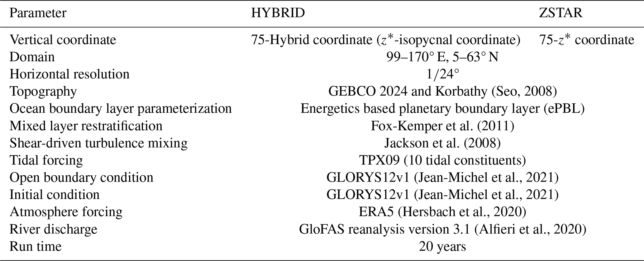
The ocean model used here is the same as that used by Chang et al. (2026a); it is based on the MOM6 (Adcroft et al., 2019) ocean model, coupled with the Sea Ice Simulator version 2 for sea ice dynamics and themodynamics. It solves the hydrostatic primitive equations using the Boussinesq approximation on an Arakawa C-grid with a horizontal resolution of $\mathrm{1}/\mathrm{24}$°. The model domain extends from 99 to 170° E and 5 to 63° N and encompassed the Northwest Pacific Ocean. Bathymetry is based on the GEBCO 2024 dataset merged with the high-resolution Korbathy dataset (Fig. 1a) (Seo, 2008). The model depths range from a minimum of 10 m, which allows for tidal variations without requiring a wetting and drying scheme, such as the one recently implemented in MOM6 (Wang et al., 2024). Time integration is performed using a split-explicit method (Hallberg, 1997; Hallberg and Adcroft, 2009), with a baroclinic time step of 300 s. The barotropic time step is chosen as the largest globally stable integer fraction of the baroclinic time step. A 900 s step is used for thermodynamic calculations. Both vertical coordinate systems used 75 layers, with the finest resolution near the surface (2 m layers down to a depth of 14 m). This vertical resolution is consistent with recent MOM6 applications in both global (Adcroft et al., 2019) and regional configurations (Ross et al., 2023; Seijo-Ellis et al., 2024; Drenkard et al., 2025; Liao et al., 2025). In the ZSTAR configuration, the layer thickness gradually increases with depth, reaching 349.43 m near the maximum model depth of 5000 m. In contrast, the HYBRID configuration uses z^* coordinates in the upper ocean and switched to isopycnal coordinates in the deeper stratified interior. The transition depth between these two systems varied with latitude (Adcroft et al., 2019). Each interface in HYBRID is assigned a target density referenced to 2000 dbar, ranging from 1010.00 to 1037.2479 kg m⁻³.

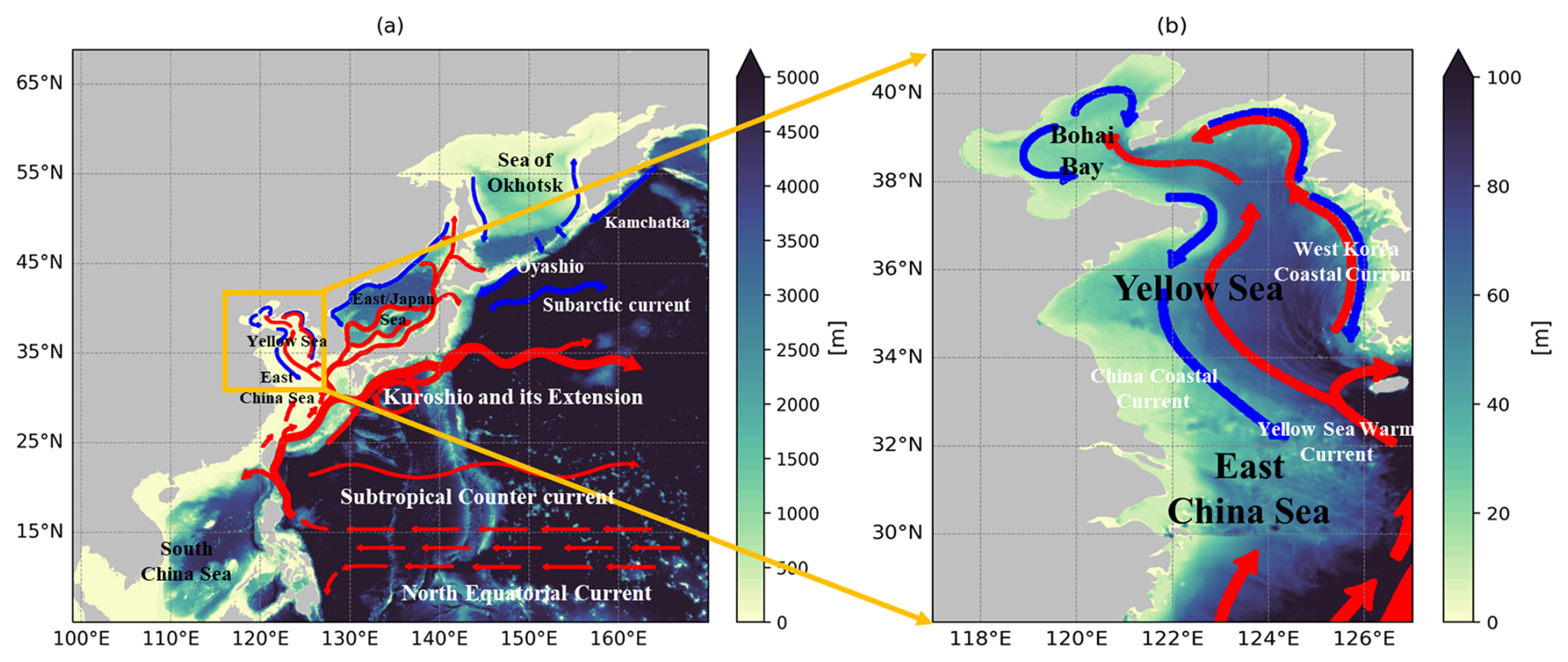
Figure 1 Model bathymetry and major surface currents in the (a) Northwest Pacific and (b) Yellow Sea. The yellow box in panel (a) indicates the regional model domain for the Yellow Sea, which is shown in greater detail in panel (b). The smaller orange dashed box in panel (b) marks the primary analysis area referenced in later figures.

The subgrid-scale parameterizations follow those of Adcroft et al. (2019) and Ross et al. (2023). The planetary boundary layer is represented using the energetics-based scheme of Reichl and Hallberg (2018) with Langmuir turbulence updates (Reichl and Li, 2019). Submesoscale restratification is parameterized by the scheme of Fox-Kemper et al. (2011) using a 1500 m frontal length scale. Horizontal viscosity is calculated using a biharmonic formulation (Griffies and Hallberg, 2000), taking the maximum of Smagorinsky viscosity and a fixed form (u₄Δx³), with u₄ = 0.01 m s⁻¹ and a Smagorinsky coefficient of 0.015. The shear-driven mixing is parameterized according to the method of Jackson et al. (2008).

Both configurations are forced with daily temperature, salinity, SSH, and velocity data from GLORYS12v1 (Jean-Michel et al., 2021). Tidal forcing is imposed using 10 tidal constituents from TPXO9 v1 (Egbert and Erofeeva, 2002), which were applied at the boundaries and as body forces. The self-attraction and loading effect was parameterized using the scalar approximation (Accad and Pekeris, 1978) with a coefficient of 0.01. The barotropic components use radiation conditions (Flather, 1976), and the baroclinic flows apply an Orlanski scheme (Orlanski, 1976) with nudging (Marchesiello et al., 2001). A reservoir scheme with a length scale of 9 km is used to determine the inflowing temperature and salinity at the open boundaries. Surface forcing is derived from hourly ERA5 reanalysis (Hersbach et al., 2020) using the bulk formula of Large and Yeager (2004). River discharge from GloFAS v3.1 (Alfieri et al., 2020) is mapped to the model grid, following Ross et al. (2023). Discharge was applied as freshwater at the surface temperature, with turbulent kinetic energy added to mix the upper 5 m.

Both configurations are initialized using the GLORYS12v1 temperature and salinity fields on 1 January 1993. A 10-year spin-up (1993–2002) is conducted using time-varying boundary and surface forcing, followed by a 10-year hindcast (2003–2012). For tidal diagnostics, analyses of barotropic and baroclinic tidal energetics are conducted using model output from the final year (2012) of the hindcast. Table 1 summarizes the model configuration and parameterizations.

Table 1 Summary of model configuration.

2.2 Observations

To assess the performance of the simulated sea surface temperature (SST) under different vertical coordinate systems in the Yellow Sea, we utilize the Operational Sea Surface Temperature and Sea Ice Analysis (OSTIA) product distributed by the Copernicus Marine Environment Monitoring Service (Good et al., 2020; https://doi.org/10.48670/moi-00165). OSTIA provides daily, gap-filled foundation SST fields derived from both satellite and in situ observations, ensuring consistency and accuracy for model validation. The product has a horizontal resolution of 0.054° and has data coverage going back to January 1981, making it suitable for evaluating SST variability in shallow tidally dynamic regions, such as the Yellow Sea. Among the available SST datasets, OSTIA performs particularly well in the Yellow Sea, with Woo and Park (2020) reporting lower errors than Daily Optimum Interpolation Sea Surface Temperature when validated against in situ measurements.

We also use observational temperature data from the Korea Oceanographic Data Center (KODC), maintained by the National Institute of Fisheries Science (NIFS). Since 1961, the NIFS has conducted oceanographic surveys around the Korean Peninsula approximately six times a year (during even-numbered months). Their observational network covers major regions such as the East/Japan Sea, Yellow Sea, and Korea/Tsushima Strait, with in situ temperature profiles reported at standard depths (0, 10, 20, 30, 50, 75, 100, 125, 150, 200, 250, 300, 400, and 500 m). In this study, only observations collected in the Yellow Sea are used to validate the vertical temperature structure of the model. The validation for salinity is excluded, as a previous study by Park (2021) reported significant time-dependent bias errors in KODC salinity records, rendering them unsuitable for model evaluation.

2.3 Diagnostic metrics

To evaluate the ability of the model to represent both barotropic and baroclinic tidal processes, a model output with at least an hourly temporal resolution is required. Given the substantial data volume associated with high-resolution simulations, only the final year (2012) of the 10-year hindcast is archived at an hourly frequency for key variables, including temperature, salinity, SSH, and three-dimensional velocity. To extract the dominant tidal signals, harmonic analysis was performed on the hourly SSH and velocity fields using the UTide Python package (Codiga, 2011), focusing on the M₂ tide, which is the dominant constituent of the Yellow Sea. Based on this output, the diagnostic metrics used in this study include the barotropic energy flux, baroclinic kinetic energy (hereafter referred to as KE), baroclinic energy flux, and barotropic-to-baroclinic conversion rate.

The barotropic tidal energy flux can be expressed by the following equation:

$$\begin{array}{}\text{(1)}& F_{\mathrm{bt}}={\mathit{\rho }}_{\mathrm{0}}g{\mathit{U}}_{\mathrm{bt}}\mathit{\eta },\end{array}$$

where ρ₀ is the reference seawater density, set to 1025 kg m⁻³ in this study; g is the gravitational acceleration; U_bt is the barotropic velocity; and η is the tidal elevation for M₂.

The depth-integrated baroclinic KE is calculated as:

$$\begin{array}{}\text{(2)}& {\mathrm{KE}}_{\mathrm{bc}}={\int }_{-H}^{\mathit{\eta }}{\mathit{\rho }}_{\mathrm{0}}(u^{{}^{\prime }\mathrm{2}}+v^{{}^{\prime }\mathrm{2}})/\mathrm{2}\mathrm{d}z,\end{array}$$

where u^′ and v^′ represent the baroclinic components of the horizontal velocity. The baroclinic velocity is derived from velocity profiles.

$$\begin{array}{}\text{(3)}& {\mathit{u}}^{\prime }\left(z,t\right)=\mathit{u}\left(z,t\right)-{\displaystyle \frac{\mathrm{1}}{H}}{\int }_{-H}^{\mathrm{0}}\mathit{u}\left(z,t\right)\mathrm{d}z\end{array}$$

Because MOM6 is fundamentally a layer model and does not explicitly provide the vertical velocity (w), the vertical component of the KE is excluded from this calculation.

As described by Kang and Fringer (2012), the baroclinic energy flux can be computed using the baroclinic velocity and the pressure perturbation, where the perturbation pressure p^′ is obtained from perturbation density ρ^′ relative to the time-averaged background field. The perturbation density is calculated as follows:

$$\begin{array}{}\text{(4)}& {\mathit{\rho }}^{\prime }=\mathit{\rho }\left(x,y,z,t\right)-{\mathit{\rho }}_{\mathrm{b}}(x,y,z),\end{array}$$

where $\mathit{\rho }\left(x,y,z,t\right)$ is the time-dependent density and ρ_b(xyz) is the time-independent background density. The perturbation pressure is calculated as follows:

$$\begin{array}{}\text{(5)}& {\displaystyle }{p}^{\prime }\left(z,t\right)=p_{\mathrm{surf}}\left(t\right)+g{\int }_z^{\mathit{\eta }}{\mathit{\rho }}^{\prime }\left(z\right)\mathrm{d}\widehat{z},\text{(6)}& {\displaystyle }{p}_{\mathrm{surf}}\left(t\right)=-{\displaystyle \frac{\mathrm{1}}{H+\mathit{\eta }}}{\int }_{-H}^{\mathit{\eta }}{\int }_Z^{\mathit{\eta }}{\mathit{\rho }}^{\prime }\left(\widehat{z,t}\right)g\mathrm{d}\widehat{z}\mathrm{d}z.\end{array}$$

Subsequently, the depth-integrated baroclinic energy flux is calculated by the following equation.

$$\begin{array}{}\text{(7)}& F_{\mathrm{bc}}={\int }_{-H}^{\mathit{\eta }}{p}^{\prime }\left(z\right)u^{\prime }\left(z\right)\mathrm{d}z.\end{array}$$

To further quantify the energy transfer from surface to internal tides, we compute the barotropic-to-baroclinic energy conversion rate, which represents the local generation of baroclinic (internal) tides via the interaction between the barotropic current and internal pressure gradients. This conversion rate can be expressed as:

$$\begin{array}{}\text{(8)}& {\displaystyle }C=\mathit{W}\cdot p^{\prime }\text{(9)}& {\displaystyle }\mathit{W}=-{\mathrm{\nabla }}_H\left[\left(h+\mathit{\eta }\right){\mathit{U}}_{\mathrm{bt}}\right]\end{array}$$

where W denotes the barotropic vertical velocity generated as the horizontal barotropic flow U_bt is forced to flow over spatial variations in the bottom topography.

The M₂ and K₁ tidal amplitudes and phases used for comparison with TPXO9 were obtained from harmonic analysis of hourly sea surface height (SSH) over a one-year period to ensure reliable estimation of the principal tidal constituents. To investigate seasonal variability, February and August were selected as representative winter and summer conditions, respectively. For each month, the diagnostic metrics are calculated using hourly outputs from the first 15 d, corresponding to approximately 29 M₂ tidal cycles, ensuring robust characterization of the semi-diurnal tidal response. To quantitatively evaluate the barotropic and baroclinic tidal responses influenced by vertical coordinate systems, spatial averages are computed over four energetic tidal regions in the Yellow Sea, as identified by Liu et al. (2019): the Yangtze River Estuary (121.8–124° E, 29.5–32° N), South Yellow Sea (122–125.8° E, 32–33.5° N), South Korean Coast (125–127° E, 33.6–36.6° N), and North Korean Coast (124–126° E, 37–39° N).

3 Results

3.1 Physical properties

Before comparing the barotropic and baroclinic tide simulations, the model representation of key physical properties, including SST and vertical temperature structure, is examined against satellite and in situ observations to ensure that the background stratification and surface conditions, which are critical factors for tidal dynamics, are reasonably captured. Figure 2 presents the spatial distribution of the mean SST and its biases relative to OSTIA in the Yellow Sea. Both the HYBRID and ZSTAR configurations capture the large-scale SST structure reasonably well and exhibit a high spatial correlation (Corr) with OSTIA (0.95 for HYBRID and ZSTAR). However, HYBRID shows superior accuracy, with a lower root mean square error (RMSE) of 0.58 °C, compared with 0.75 °C for ZSTAR. While both models exhibit a warm bias (< 1.0 °C) in the western Yellow Sea and a cool bias along the southeastern margin, ZSTAR additionally displays an extensive cold bias throughout the southern Yellow Sea.

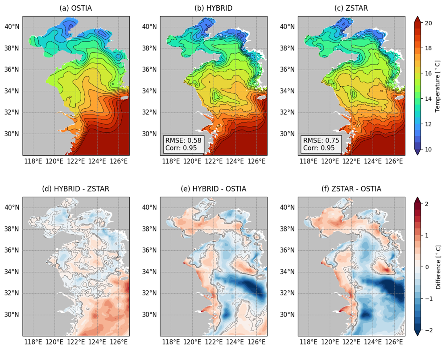
Figure 2 Annual mean sea surface temperature (SST) distributions from OSTIA and the HYBRID and ZSTAR simulations in the Yellow Sea for 2012. Panels (a)–(c) display the spatial distributions of SST, along with their root mean square error (RMSE) and correlation (Corr). Panel (d) presents the differences between HYBRID and ZSTAR, and panels (e) and (f) illustrate the biases relative to OSTIA. Contour lines in (d)–(f) indicate SST biases ranging from −0.1 to 0.1 °C at 0.1 °C intervals.

To compare the representations of the temperature field under weakly and strongly stratified conditions, the validation period is divided into two seasonal groups (Fig. 3). Because the NIFS collects in situ temperature profiles around the Korean Peninsula only during even-numbered months, the validation is conducted using data from February, April, and December (FAD) to represent weak stratification and from June, August, and October (JAO) to represent strong stratification. For each season, the depth-averaged temperature bias and RMSE are computed to evaluate the performance of the HYBRID and ZSTAR configurations. During the weakly stratified season (FAD; Fig. 3a and b), both configurations exhibit a warm bias across the domain, particularly in the southern region. However, ZSTAR displays a stronger warm bias, with temperatures exceeding those of HYBRID by approximately 0.5 °C. In contrast, during the strongly stratified season (JAO, Fig. 3c–d), ZSTAR exhibits a pronounced cold bias exceeding −3.0 °C in the central Yellow Sea, while simultaneously showing a warm bias along the Korean coastal region. HYBRID, however, displays consistently reduced biases in both the offshore and nearshore regions, suggesting a more balanced and realistic vertical temperature distribution. The RMSE distributions (Fig. 3e–h) further support these findings. ZSTAR tends to produce larger errors across the section, especially during JAO, when stratification is strong, with peak RMSEs surpassing 2.5 °C. In contrast, HYBRID maintains relatively low RMSE values across most latitudinal bands and depths. This result highlights the superior ability of HYBRID in reproducing vertical thermal structures under various stratification conditions.

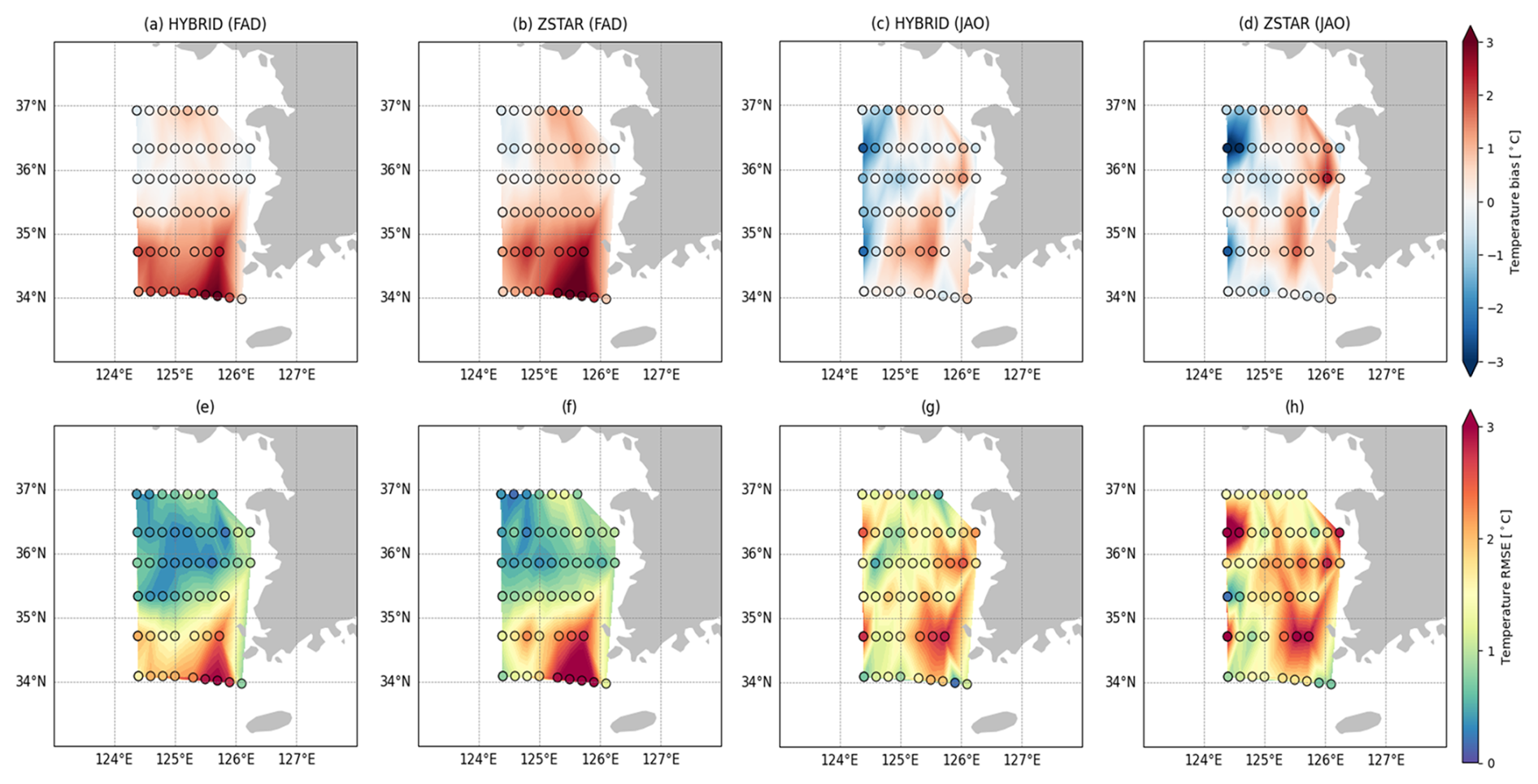
Figure 3 Spatial distribution of the depth-averaged bias and RMSE in model-simulated temperature with respect to the in situ temperature profile obtained from the Korea Oceanographic Data Center (KODC) in the Yellow Sea for the 2012 year. Panels (a)–(d) show temperature bias (°C) for HYBRID and ZSTAR during FAD (February, April, and December; (a–b) and JAO (June, August, and October; c–d). Panels (e)–(h) present the corresponding root-mean-square error (RMSE, °C) distributions for each configuration and season.

The vertical temperature structure in August, when stratification in the Yellow Sea is strongest, is generally well reproduced by both configurations, although noticeable deviations from the observations remain (Fig. 4). HYBRID tends to align more closely with the observed profile than ZSTAR across much of the water column, particularly within the thermocline (approximately 10–40 m depth), where strong vertical gradients occur (Fig. 4a). Although ZSTAR also captures the overall stratification, it exhibits somewhat larger deviations in this depth range and shows a slightly broader spread in its ensemble representation, implying greater vertical variability than observed.

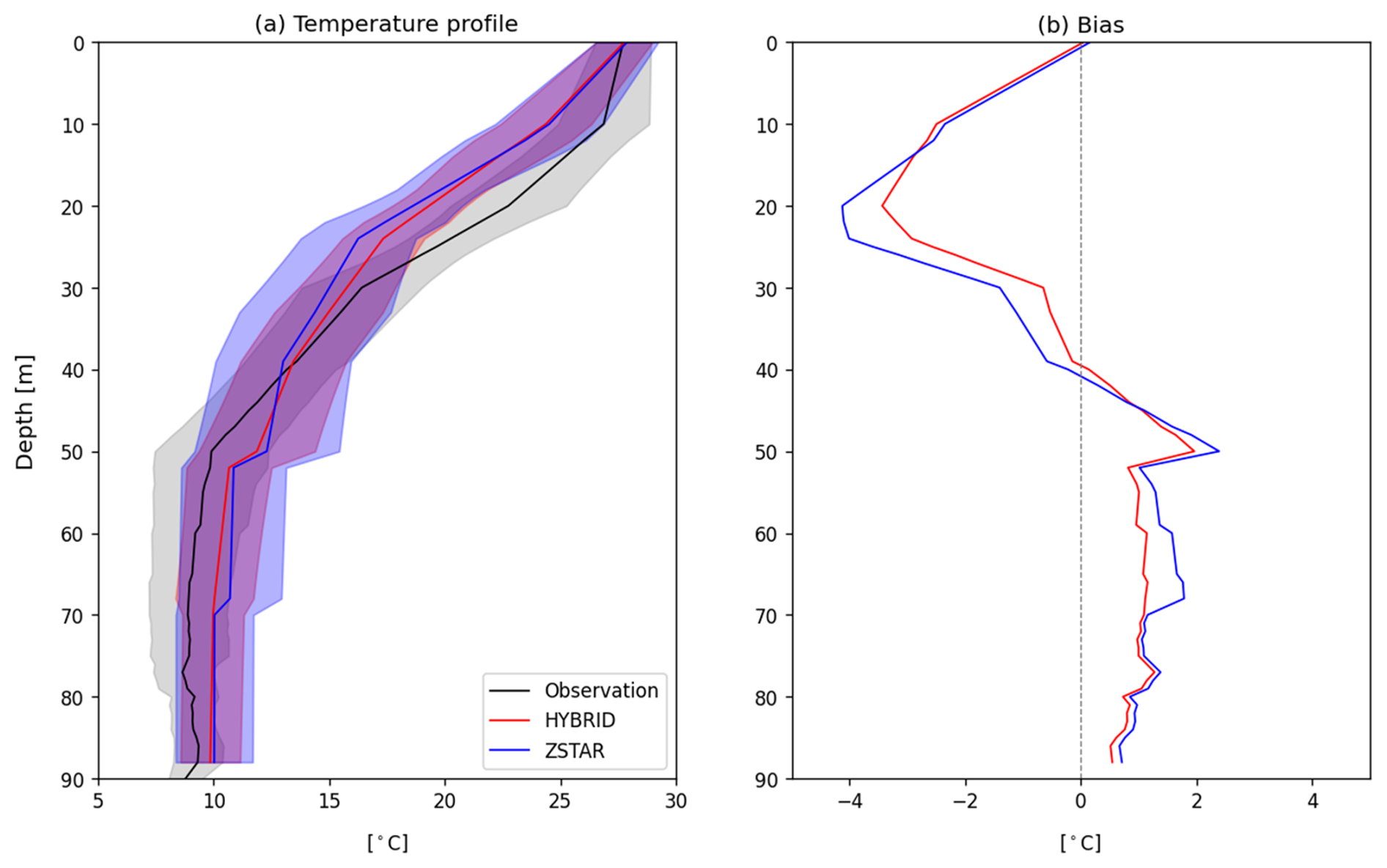
Figure 4 Spatial mean vertical temperature profiles and their biases with respect to the in situ temperature profile obtained from the KODC in the Yellow Sea during August. Panel (a) shows the mean temperature profiles from observations (black), HYBRID (red), and ZSTAR (blue), with the shaded areas representing one standard deviation (±1σ) around the mean. Panel (b) displays the corresponding temperature bias (model – observation) for HYBRID and ZSTAR.

The corresponding bias profiles (Fig. 4b) further indicate that both configurations show cold biases in the upper layer and warm biases below the thermocline. However, ZSTAR generally shows larger absolute biases, exceeding −4 °C locally in the upper 40 m, whereas HYBRID shows relatively smaller biases throughout the water column. Although the differences between the two configurations are not dramatic, these results suggest that HYBRID provides a somewhat improved representation of the sharp summer stratification and the associated thermal structure in this shelf-sea environment.

The spatial distribution of the depth-averaged buoyancy frequency in February and August indicates notable seasonal differences in stratification between the HYBRID and ZSTAR configurations (Fig. 5). In February, both configurations show low buoyancy frequency across most of the Yellow Sea, reflecting weak stratification associated with strong wintertime vertical mixing (Fig. 5a–b). In contrast, the buoyancy frequency increases substantially in August (Fig. 5d–e), particularly in the central Yellow Sea regions as well as in Bohai Bay and the Yangtze River Estuary, reflecting the development of a seasonal thermocline under surface heating and freshwater-induced stratification. The difference maps (Fig. 5c and f) highlight the systematic variations between the two configurations. In August, although HYBRID shows slightly weaker stratification in some localized regions, it produces higher buoyancy frequency in areas where summer stratification is strongly developed, particularly where freshwater input intensifies stratification, indicating that HYBRID captures the enhanced seasonal stratification more effectively than ZSTAR. This contrast is less pronounced in February, which is consistent with the generally well-mixed state of the winter water column. The stronger summer stratification simulated by HYBRID in the central Yellow Sea and near the Korean Coast is likely more reliable because HYBRID demonstrates improved agreement with the observed temperature profiles and reduced bias in these regions (Figs. 3 and 4). Given that the buoyancy frequency is directly derived from the vertical temperature gradient, the better simulation of the temperature fields by HYBRID suggests that its representation of stratification in these areas is also more accurate. In contrast, no direct observational comparison is conducted for the Yangtze River Estuary region in this study. Therefore, although HYBRID simulates stronger stratification in this area, this result should be interpreted with caution. Nevertheless, the enhanced buoyancy frequency may reflect the improved capability of HYBRID to capture freshwater-induced density gradients near river outflows, a behavior that warrants further investigation using dedicated observational datasets. Collectively, these results suggest that the choice of vertical coordinate system can significantly influence the simulation of stratification in shelf regions, particularly under strong surface forcing and freshwater input.

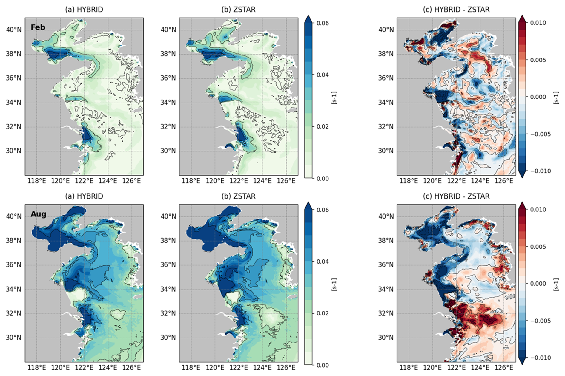
Figure 5 Spatial distribution of the depth-averaged buoyancy frequency in the Yellow Sea during February (top row) and August (bottom row). Panels (a) and (d), (b) and (e) show the buoyancy frequencies from the HYBRID and ZSTAR configurations, respectively. Panels (c) and (f) present the difference between the two configurations (HYBRID–ZSTAR).

3.2 Barotropic tides

Barotropic tides, which represent the nearly depth-independent component of tidal motion, are the dominant tidal signals across the shallow Yellow Sea, and play a key role in driving horizontal transport and bottom frictional dissipation. Their accurate simulation is essential for resolving coastal sea level variability, tidal mixing, and energy dissipation processes. We evaluate the performance of the HYBRID and ZSTAR vertical coordinate systems in simulating the semidiurnal M₂ and diurnal K₁ barotropic tides. In addition, barotropic energy fluxes are diagnosed specifically for the dominant M₂ constituent to examine how each configuration captured the generation and propagation of tidal energy across the Yellow Sea Basin, as well as the differences in the magnitude and spatial distribution of energy transport.

The M₂ tidal amplitudes and phases in the Yellow Sea from the HYBRID and ZSTAR configurations are compared with those from the TPXO9 tidal model (Fig. 6). Both configurations broadly capture the amphidromic system centered near 124° E, 35° N, as well as the large-scale amplitude distribution. However, HYBRID shows better agreement with TPXO, achieving a lower RMSE (24.19 cm) and higher spatial correlation (0.76) than ZSTAR (RMSE: 32.55 cm, Corr: 0.67), indicating improved tidal performance. In terms of amplitude bias (Fig. 6d–f), HYBRID simulated higher M₂ amplitudes than ZSTAR across much of the basin, with the largest differences appearing along the Korean coast. Compared with TPXO, HYBRID exhibits smaller overall errors, whereas ZSTAR tends to underestimate amplitudes near the Korean Peninsula, with errors exceeding −40 cm in some regions.

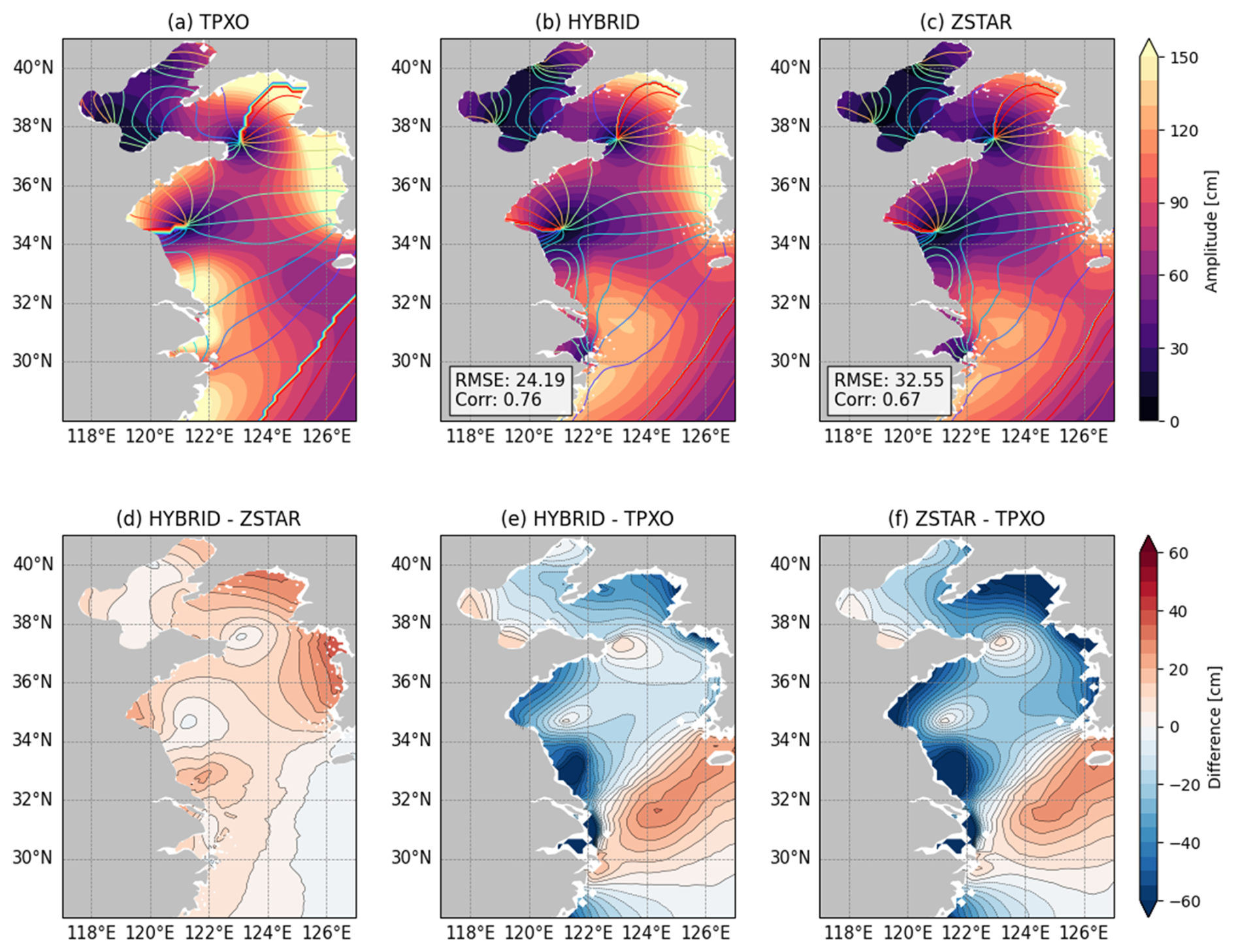
Figure 6 Spatial distribution of the semidiurnal M₂ tidal amplitude and phase from (a) TPXO9, (b) HYBRID, and (c) ZSTAR in the Yellow Sea. Shaded contours indicate amplitude (cm) and colored lines denote phase. Panels (d)–(f) show amplitude differences: (d) HYBRID – ZSTAR, (e) HYBRID – TPXO, and (f) ZSTAR – TPXO. The spatial RMSE and Corr between each model and TPXO are also provided to quantify model performance.

The diurnal K₁ tide exhibited a similar pattern (Fig. 7). Both HYBRID and ZSTAR broadly reproduce the observed amphidromic structure centered near 123.5° E, 34° N, as represented in the TPXO. However, HYBRID demonstrates better agreement in terms of amplitude and phase, achieving a lower RMSE (4.72 cm) than ZSTAR (5.70 cm), indicating improved tidal accuracy. Amplitude difference maps reveal that ZSTAR tended to underestimate K₁ amplitudes across much of the basin, with negative biases reaching up to −10 cm in several regions.

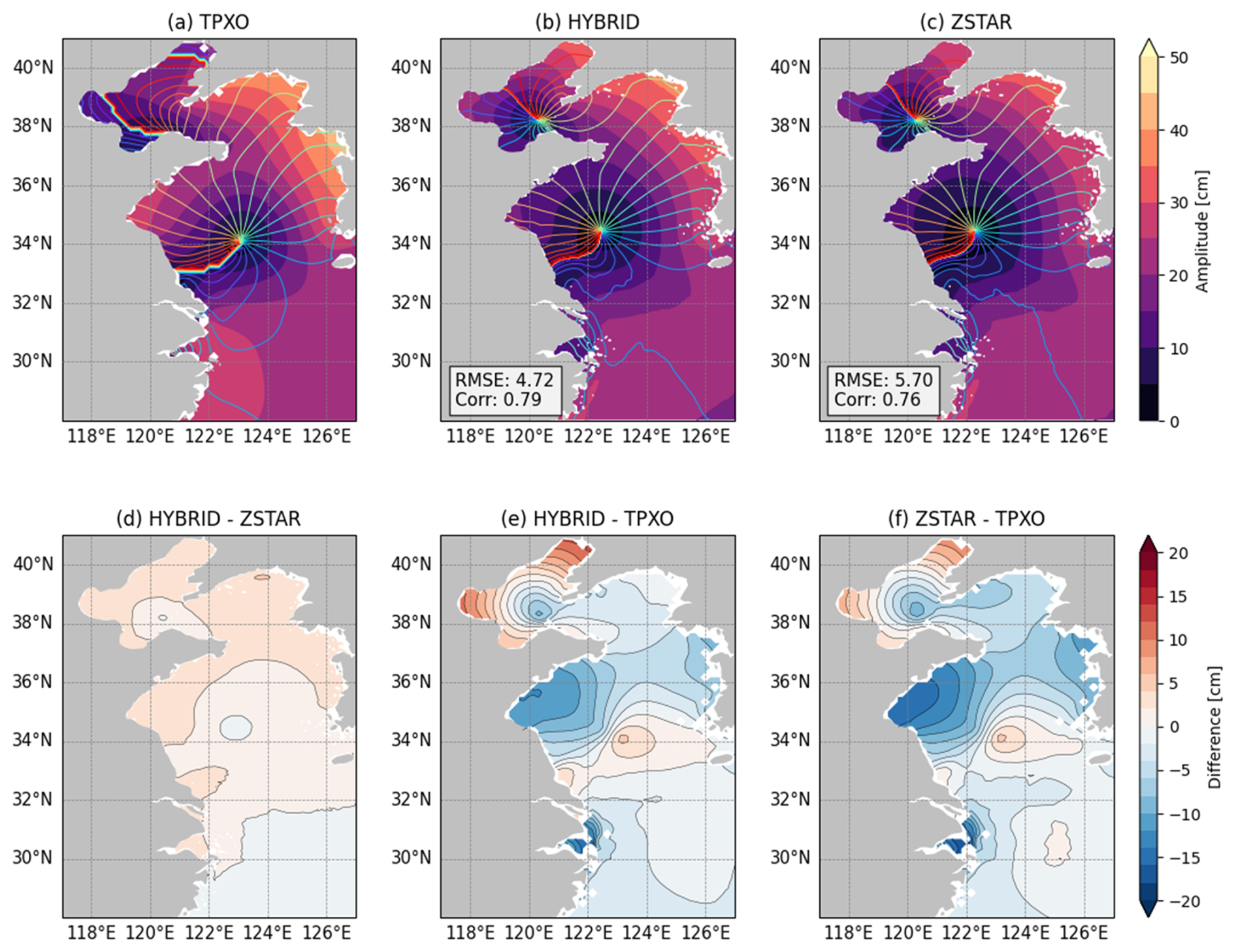
Figure 7 Spatial distribution of the diurnal K₁ tidal amplitude and phase from (a) TPXO9, (b) HYBRID, and (c) ZSTAR in the Yellow Sea. Shaded contours indicate amplitude (cm) and colored lines denote phase. Panels (d)–(f) show amplitude differences: (d) HYBRID – ZSTAR, (e) HYBRID – TPXO, and (f) ZSTAR – TPXO. The spatial RMSE and Corr between each model and TPXO are also provided to quantify model performance.

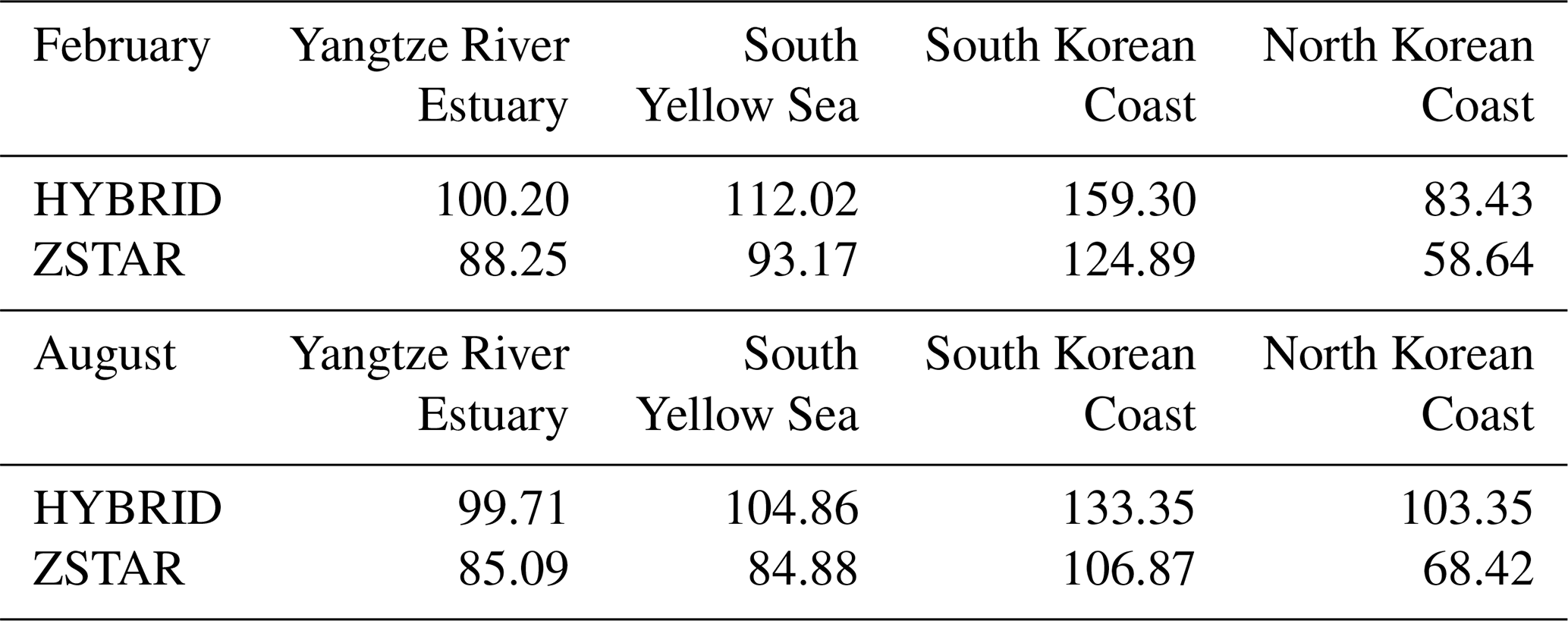
Because the M₂ tide is the dominant tidal constituent in the Yellow Sea and exhibits the most pronounced differences between configurations, subsequent analyses focused on the M₂ component for harmonic decomposition and comparison. The barotropic tidal energy flux vectors and magnitudes associated with the M₂ constituent in the Yellow Sea show a similar large-scale propagation pattern in both HYBRID and ZSTAR during February and August (Fig. 8). In both configurations, tidal energy propagates from southeast to northwest and dissipates over the shallow shelf. In February (Fig. 8a–b), when the water column is well mixed, the overall energy pathways are broadly similar between the two configurations. However, HYBRID exhibits systematically stronger flux magnitudes across all four tidal regions (Table 2). Quantitative comparisons show that HYBRID produced a 13.5 % larger flux in the Yangtze River Estuary, 20.2 % larger flux in the South Yellow Sea, 27.6 % larger flux along the South Korean Coast, and 42.3 % larger flux along the North Korean Coast, relative to ZSTAR. In August (Fig. 8d–e), when the water column becomes strongly stratified, both configurations simulated a general weakening of the barotropic energy flux, especially in the central basin, which may be attributed to the enhanced energy conversion from barotropic to baroclinic tides under strong summer stratification (Kang et al., 2002). Nevertheless, HYBRID continues to produce stronger energy flux magnitudes than ZSTAR across all four regions, yielding a 17.2 % higher flux in the Yangtze River Estuary, 23.5 % higher flux in the South Yellow Sea, 24.8 % higher flux along the South Korean Coast, and 51.1 % higher flux along the North Korean Coast. These results further support the hypothesis that the HYBRID configuration preserves barotropic tidal energy more effectively under both weakly and strongly stratified conditions.

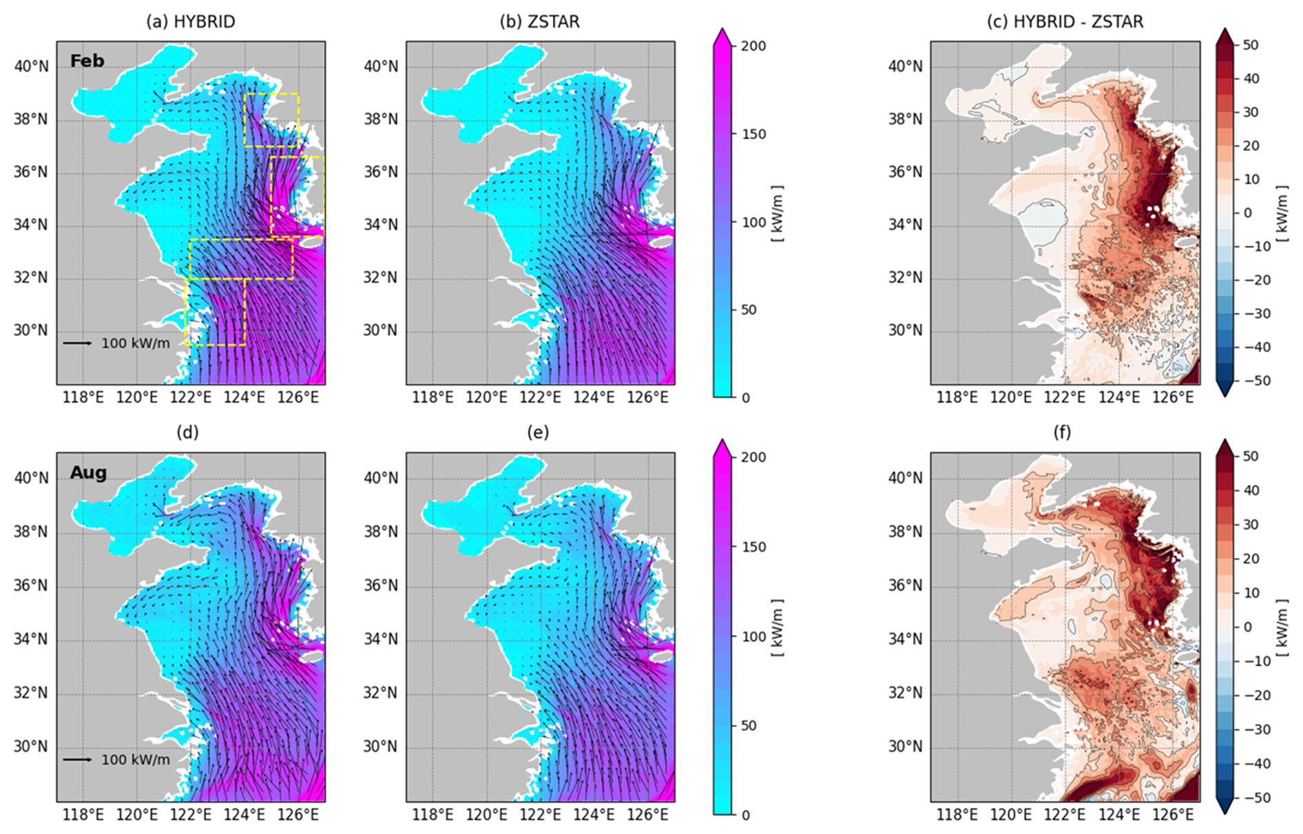
Figure 8 Barotropic tidal energy flux vectors and its magnitudes for the M₂ constituent in the Yellow Sea, calculated from the first 15 d of each month's simulation. Panels (a)–(b) show fluxes and magnitudes for February and panels (d)–(e) for August, as simulated by HYBRID (left) and ZSTAR (right). Panels (c) and (f) present the differences in barotropic tidal energy magnitudes between HYBRID and ZSTAR. Arrows indicate the direction and magnitude of energy flux (units in kW m⁻¹). The yellow boxes in panel (a) denote four energetic tidal regions used for quantitative evaluation through spatial averaging.

Table 2 Spatially averaged barotropic tidal energy flux magnitudes (kW m⁻¹) for the M₂ constituent in four energetic tidal regions of the Yellow Sea, calculated over the first 15 d of simulation in February and August. Values are presented for both the HYBRID and ZSTAR configurations.

3.3 Baroclinic tides

Although barotropic tides dominate shallow regions of the Yellow Sea, internal (baroclinic) tides play critical roles in subsurface energy propagation and vertical mixing, particularly during periods of strong stratification. Given the marked seasonal stratification in the Yellow Sea, especially in summer, internal tide generation and propagation are expected to vary significantly with the season and vertical coordinate representation. To assess the performance of the model in simulating baroclinic tides, we analyze diagnostics such as the baroclinic KE and energy flux associated with the M₂ constituent.

The spatial distribution of the depth-integrated baroclinic KE for the M₂ tidal constituent in the Yellow Sea for February and August is compared between the HYBRID and ZSTAR configurations (Fig. 9). In both seasons, pronounced baroclinic KE maxima consistently appear near the Yangtze River Estuary and in regions characterized by steep topographic gradients. These areas are well-known hotspots for internal tide generation associated with strong barotropic-to-baroclinic energy conversion over rough topography. In addition, the Yellow Sea lies close to the critical latitude (∼ 30° N) of the diurnal K₁ tide, where the tidal frequency approaches the local inertial frequency, favoring enhanced internal wave activity (Dong et al., 2019). Consequently, enhanced baroclinic KE is also observed around 30–32° N. Such dynamical conditions can further intensify internal wave responses and contribute to the amplification of M₂ internal tides, a tendency that is also evident in Fig. 9.

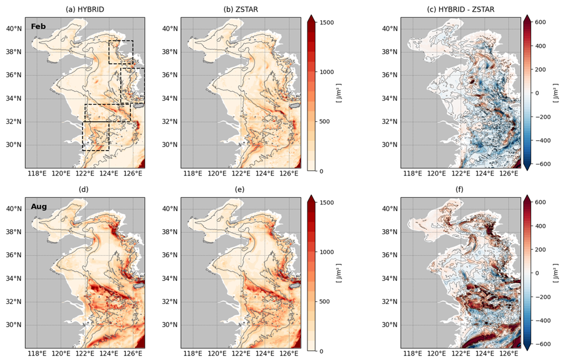
Figure 9 Depth-integrated baroclinic kinetic energy (J m⁻²) for M₂ simulated by HYBRID and ZSTAR in the Yellow Sea, calculated from the first 15 d of each month's simulation. Panels (a)–(b) and (d)–(e) show the February and August distributions for each configuration, respectively. Panels (c) and (f) present the differences between HYBRID and ZSTAR. The gray contours represent the 20, 50, and 80 m isobaths. The black boxes in panel (a) denote four energetic tidal regions used for quantitative evaluation through spatial averaging.

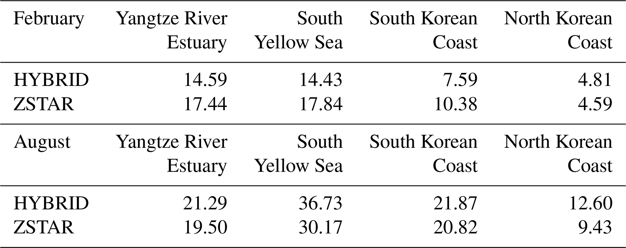
In February (Fig. 9a–c), the baroclinic KE remains relatively low across most of the basin owing to weak stratification. However, the difference maps (Fig. 9c) reveal that ZSTAR tends to produce a higher baroclinic KE than HYBRID over much of the southern shelf, quantitatively exhibiting approximately 19.5 % and 23.6 % greater KE in the Yangtze River Estuary and South Yellow Sea, respectively (Table 3). Along the South Korean and North Korean coasts, the differences are smaller, with nearly identical values in the latter region. Given the overall weak stratification in winter, the enhanced baroclinic KE in ZSTAR might be attributable to spurious energy conversion or numerical noise rather than physically realistic internal tide processes. In contrast, the August distribution (Fig. 9d–f) shows a marked increase in the baroclinic KE, which is consistent with the development of strong summer stratification and active internal tide generation. During this season, HYBRID simulates a higher baroclinic KE than ZSTAR across all four evaluation regions. HYBRID produces 21.7 % greater KE in the South Yellow Sea and 33.6 % greater KE along the North Korean Coast and exceeded the ZSTAR in the Yangtze River Estuary by 9.2 % and 5.0 % on the South Korean Coast. These regional enhancements align with areas of elevated buoyancy frequency (Fig. 5f), particularly along the Korean coast and estuarine fronts, supporting the interpretation that HYBRID captures the barotropic-to-baroclinic energy conversion processes more effectively under strong stratification conditions.

Table 3 Spatial and depth-integrated baroclinic kinetic energy (TJ) for the M₂ tidal constituent in four energetic tidal regions of the Yellow Sea, calculated from the first 15 d of simulation in February and August. Values are presented for both the HYBRID and ZSTAR configurations.

The baroclinic tidal energy flux vectors associated with the M₂ tide in the Yellow Sea during February and August reveal clear seasonal differences (Fig. 10). In February, both configurations simulate relatively weak and spatially limited fluxes, consistent with the low baroclinic KE shown in Fig. 9a–b. Most energy fluxes are localized near steep topographic features, particularly along the southern Korean coast and near the Yangtze River Estuary. HYBRID and ZSTAR exhibited broadly similar patterns, although ZSTAR exhibited slightly more scattered flux vectors. In August (Fig. 10c, d), when stratification is strong, the differences between the two configurations become more pronounced. HYBRID generates stronger and more spatially extensive baroclinic energy fluxes throughout the central Yellow Sea, along the Korean coastal shelf, and near the estuarine front of the Yangtze River. These areas coincide with the enhanced baroclinic KE shown in Fig. 9. Coherent flux directions and widespread coverage indicate more efficient internal tide generation and propagation in HYBRID. In contrast, ZSTAR produces weaker, patchier fluxes with reduced spatial reach, suggesting a limited conversion of barotropic to baroclinic energy.

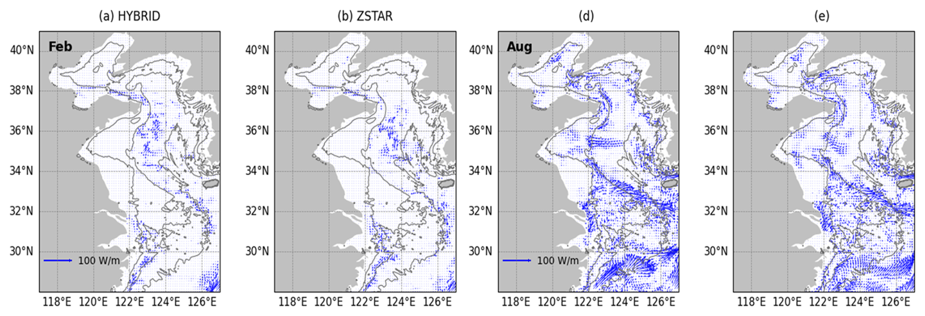
Figure 10 Baroclinic tidal energy flux vectors for the M₂ constituent in the Yellow Sea, calculated from the first 15 d of each month's simulation. Panels (a)–(b) show the fluxes for February and panels (c)–(d) for August, as simulated by the HYBRID (left) and ZSTAR (right) configurations. Arrows indicate the direction and magnitude of energy flux (vector units in W m⁻¹).

To explicitly assess how internal tides, manifest in the vertical density structure, we analyze the time evolution of the potential density and surface M₂ amplitude over a 24 h period (Fig. 11) at a central location in the Yellow Sea (124° E, 36° N) during summer (8 August). This location is selected because it features a relatively deep bathymetry within the Yellow Sea and is influenced by the YSBCW, which plays a key role in the propagation and trapping of internal tides during the stratified summer.

In the HYBRID simulation (Fig. 11a), clear internal tidal signals emerge throughout the stratified water column. The M₂ oscillations are evident at depths of approximately 10–15 and 20–30 m, consistent with the internal gravity wave-induced vertical displacements of the isopycnals. The stratification in this region supports the trapping and vertical propagation of baroclinic wave energy, and the alternating isopycnal deflections exhibit a well-organized structure. Coherent oscillations also appear near the bottom (below 50 m), indicating downward propagation of the internal tide energy and its interaction with the YSBCW layer. These vertical fluctuations are largely in phase with the surface M₂ cycle, suggesting efficient barotropic-to-baroclinic energy conversion and vertical energy transfer across the water column. In contrast, the ZSTAR configuration (Fig. 11b) shows significantly weaker vertical displacements of the isopycnals. Although the M₂-period oscillations are subtly visible in the upper 30 m, they are less coherent and shallower in penetration than those in HYBRID. The lower portion of the water column remained almost undisturbed, and no significant internal tide signatures are observed near the bottom despite the presence of stratification. This indicates that the internal tidal energy generated at the surface or slope regions does not efficiently propagate downward.

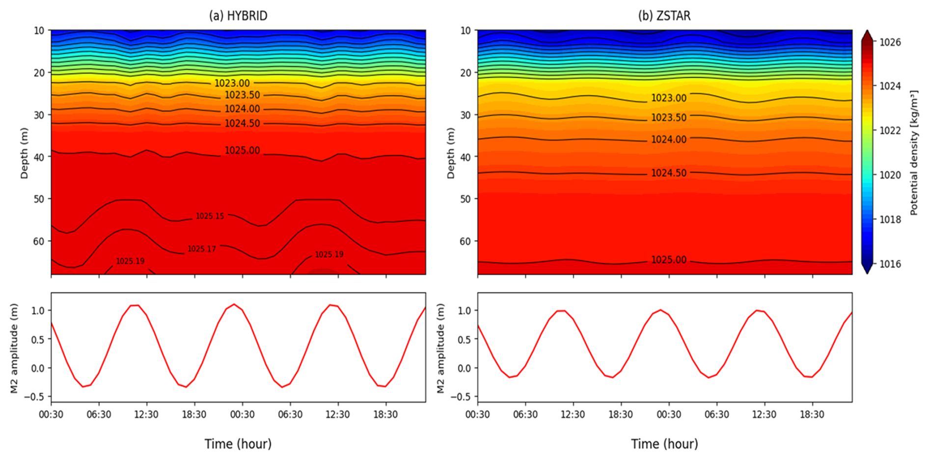
Figure 11 Time evolution of the potential density (top) and surface M₂ amplitude (bottom) at a central location in the Yellow Sea (124° E, 36° N) from the HYBRID and ZSTAR simulation on 8 August.

To further clarify the underlying mechanisms responsible for the differences in the baroclinic energy intensity and vertical structure between the two configurations, we examine the barotropic-to-baroclinic energy conversion rate, which directly quantifies the generation of internal tidal energy from barotropic tidal forcing in the presence of stratification and bathymetry. As a key diagnostic tool, this term reveals where and how efficiently the barotropic tidal energy is transformed into baroclinic motion across the model domain. Figure 12 illustrates the spatial distribution of the conversion rates for February and August, highlighting the localized regions of strong energy transfer, particularly along steep topographic gradients and near shelf break zones.

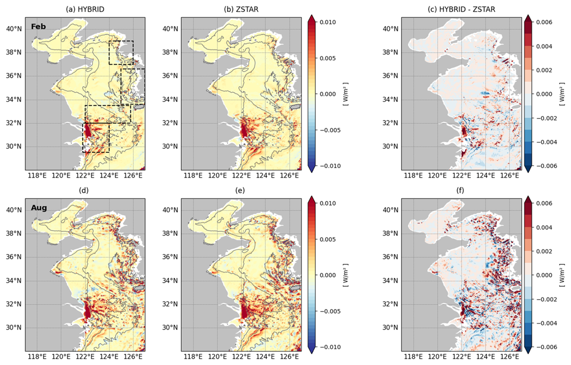
Figure 12 Depth-integrated barotropic to baroclinic energy conversion (W m⁻²) for M₂ simulated by HYBRID and ZSTAR in the Yellow Sea, calculated from the first 15 d of each month's simulation. Panels (a)–(b) and (d)–(e) show the February and August distributions for each configuration, respectively. Panels (c) and (f) present the differences between HYBRID and ZSTAR. The gray contours represent the 20, 50, and 80 m isobaths. The black boxes in panel (a) denote four energetic tidal regions used for quantitative evaluation through spatial averaging.

In February, when stratification is weak, both HYBRID and ZSTAR exhibit spatially patchy and generally weak barotropic-to-baroclinic conversion across the Yellow Sea (Fig. 12a–c). Negative or near-zero conversion dominates most of the basin, indicating that wintertime internal-tide generation is highly suppressed under weak stratification. Nevertheless, the Yangtze River Estuary remains a primary hotspot due to strong tidal forcing and steep bathymetry, where both configurations show similarly large conversion magnitudes (143.85 MW in HYBRID vs. 144.84 MW in ZSTAR; Table 4). Outside the estuary, however, regional contrasts emerge: ZSTAR produces noticeably stronger conversion in the South Yellow Sea (+30.5 % relative to HYBRID) and more than triple the conversion along the South Korean Coast (+292.2 %), while HYBRID shows slightly greater conversion near the North Korean Coast. Despite these differences, the basin-wide baroclinic KE remains similarly weak in both configurations (Table 3), underscoring that winter internal-tide energetics are primarily controlled by bathymetric forcing rather than stratification-driven processes. As a result, both configurations convert barotropic tidal energy at broadly comparable levels during winter.

Table 4 Spatial and depth-integrated barotropic to baroclinic conversion rate (MW) for the M₂ tidal constituent in four energetic tidal regions of the Yellow Sea, calculated from the first 15 d of simulation in February and August. Values are presented for both the HYBRID and ZSTAR configurations.

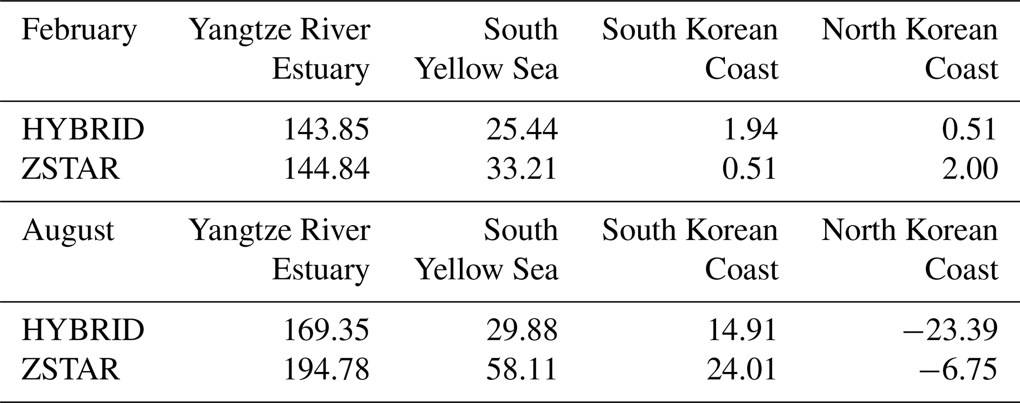
In contrast, in August, strong stratification substantially enhances barotropic-to-baroclinic conversion in both configurations (Fig. 12d–e). The Yangtze River Estuary and South Yellow Sea remain the dominant generation hotspots; however, the performance contrast between HYBRID and ZSTAR becomes far more pronounced under these strongly stratified summer conditions. Compared to HYBRID, ZSTAR exhibits a 15.0 % increase in conversion in the Yangtze River Estuary and nearly double (+94.5 %) the conversion in the South Yellow Sea. Along the South Korean Coast, ZSTAR also shows 61.1 % stronger conversion, while conversion near the North Korean Coast shifts from negative values in HYBRID to a moderately positive level in ZSTAR (Table 4). Despite these substantially enhanced conversion magnitudes, ZSTAR produces weaker baroclinic KE and less coherent internal-tide propagation than HYBRID (Figs. 9–11), indicating that a large fraction of the baroclinic energy generated in ZSTAR is rapidly dissipated or trapped locally, rather than radiated outward as sustained internal tides.

This contrasting behavior can be more clearly interpreted through the baroclinic energy budget. Although ZSTAR generates substantially greater barotropic-to-baroclinic conversion in August, the resulting baroclinic KE and baroclinic energy flux remain weaker than those in HYBRID (Figs. 9–11), demonstrating that only a limited portion of the converted energy is radiated away as coherent internal tides. From the depth-integrated and time-mean baroclinic energy balance,

$$<{\mathrm{\nabla }}_H\cdot F_{\mathrm{bc}}>=<C>-<D>,$$

where ∇_H⋅F_bc is the divergence of baroclinic energy flux, C represents the barotropic-to-baroclinic conversion, and D denotes the dissipation of baroclinic tidal energy.

The strong local damping of internal tide energy in the Yellow Sea has also been reported in previous studies. For example, Liu et al. (2019) demonstrated that internal-tide dissipation is nearly equivalent to barotropic-to-baroclinic conversion over most of the basin, indicating that only a small fraction of the converted energy can radiate away from the generation regions. Our results exhibit a highly consistent behavior: because the divergence of the baroclinic energy flux remains relatively weak over the shallow and frictionally dominated Yellow Sea, the spatial pattern of dissipation $<D>=<C>-<{\mathrm{\nabla }}_H\cdot F_{\mathrm{bc}}>,$ closely follows that of conversion in both configurations. Therefore, we do not present dissipation maps separately, as these would provide redundant information without adding physical insight. Instead, we assess dissipation through the regional baroclinic energy budget, which clearly indicates that when the radiated baroclinic energy flux remains weak, the greater conversion in ZSTAR inevitably appears as a larger dissipation term. This implies that much of the additional baroclinic energy generated in ZSTAR is rapidly removed locally, through enhanced damping or numerical mixing, rather than contributing to propagating internal tides. Consequently, HYBRID facilitates more coherent propagation of internal tides away from the generation regions, while ZSTAR loses a larger fraction of the converted energy locally due to limited radiation efficiency. These contrasting energy pathways form the basis for further investigation of the underlying physical drivers, which are examined in the Discussion section.

4 Discussion

The results presented in this study collectively suggest that, compared with ZSTAR, the HYBRID configuration exhibits superior skill in simulating barotropic tides and baroclinic tidal dynamics in the Yellow Sea. This performance gap appears to be strongly linked to the differences in the representation of summer stratification between the two vertical coordinate systems. HYBRID can maintain a stronger and more realistic stratification during the summer months, which is a crucial prerequisite for the generation and propagation of internal tides. This is further supported by a comparative evaluation against observational datasets, with HYBRID consistently outperforming ZSTAR in reproducing the SST and vertical thermal structure, particularly during the strongly stratified season. The ability of HYBRID to maintain stronger summer stratification is likely attributable to its superior control of vertical mixing and interior water mass ventilation, as demonstrated by the results of an experiment conducted by Chang et al. (2026a). In this experiment, an idealized age tracer is initialized and tracked following a spin-up simulation to quantify the rate of water mass renewal and subduction. The tracer increases linearly with time in the absence of ventilation, allowing a clear diagnosis of the vertical exchange processes. A 10-year integration was conducted for both HYBRID and ZSTAR, enabling a comparative assessment of the ventilation efficiency and stratification maintenance in the central Yellow Sea. Figure 13 shows the seasonal evolution of the age tracer and water temperature distributions at a fixed location (124° E, 36° N) in the central Yellow Sea, where well-developed cold bottom waters and strong summer stratification significantly influence internal tide dynamics, resulting in clear differences in subsurface and bottom-layer internal tide propagation between HYBRID and ZSTAR (Fig. 11).

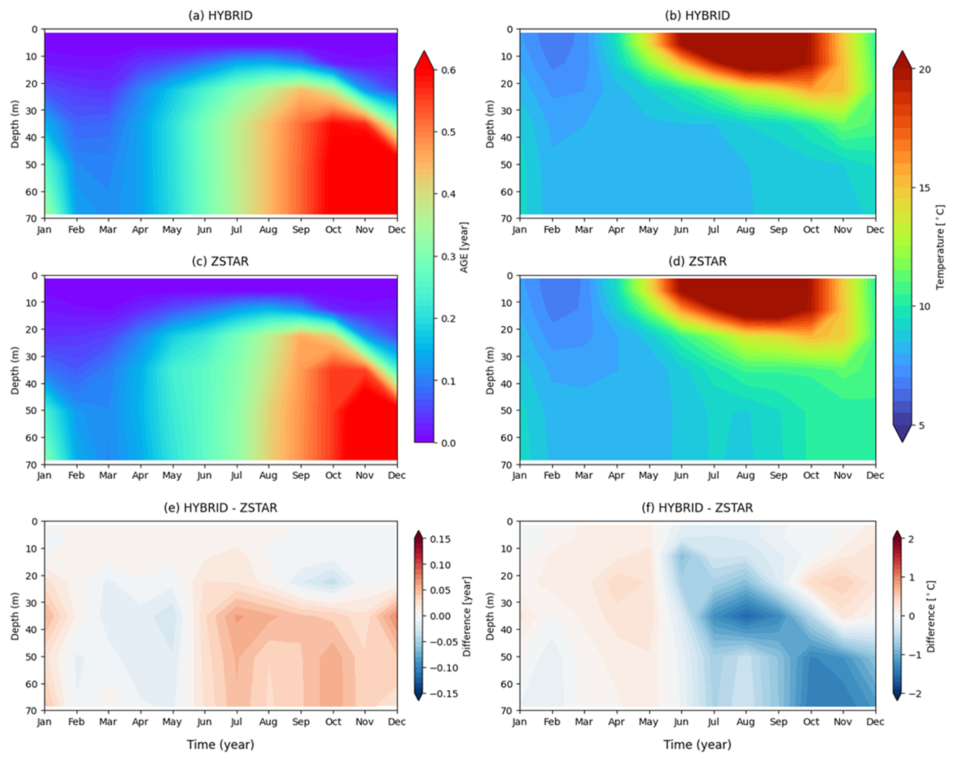
Figure 13 Seasonal evolution of age tracer (left) and temperature (right) at a fixed location in the central Yellow Sea (124° E, 36° N) based on monthly climatology over a 10-year period (2003–2012). Panels (a)–(b) show results from HYBRID and panels (c)–(d) show the corresponding fields from ZSTAR. Panels (e)–(f) present the differences between HYBRID and ZSTAR (HYBRID – ZSTAR) for the age tracer and temperature, respectively.

In HYBRID (Fig. 13a), older water masses persist below the thermocline throughout the summer and fall, indicating limited vertical exchange and weaker surface-driven ventilation. The stratified structure is particularly evident from summer to autumn (JJA–SON), with older tracer ages extending from 30 to 60 m depth. In contrast, ZSTAR (Fig. 13c) systematically exhibits younger water throughout the water column, especially during the stratified seasons, suggesting stronger vertical mixing that disrupted tracer retention and eroded the thermocline. The age difference reaches up to 0.08 years (approximately 29.2 d), indicating that ZSTAR promotes a more active upward mixing of deeper waters, which contributes to a weaker and less persistent stratification.

This difference in vertical mixing behavior is further supported by the seasonal distribution of water temperature (Fig. 13b, d). During summer (JJA), HYBRID (Fig. 13b) maintains a cooler and more stable subsurface layer, with a sharp thermocline observed below 20–30 m. In contrast, ZSTAR (Fig. 13d) shows a warmer and more diffused vertical structure, which is indicative of thermocline erosion and stronger upward mixing. The temperature difference plot (Fig. 13f) highlights that HYBRID is consistently cooler than ZSTAR between 20 and 50 m during the stratified seasons, with peak differences exceeding −1.0 °C in late summer. This cooling is consistent with suppressed diapycnal mixing and better preservation of the thermal gradient, allowing HYBRID to maintain a more realistic stratified water column in the central Yellow Sea.

To further investigate the mechanisms underlying the differences in stratification between the HYBRID and ZSTAR configurations, we examine the spatial distribution of shear-driven diapycnal mixing, which plays a key role in eroding stratification by enhancing the vertical exchange. Figure 14 presents the depth-averaged shear-driven diapycnal diffusivity for February and August, comparing HYBRID and ZSTAR. The quantitative comparison is summarized in Table 5. During the winter (February; Fig. 14a–c), when stratification is weak, both configurations exhibit relatively high diapycnal mixing over much of the basin. However, ZSTAR shows systematically greater diffusivities, with increases of 20.2 % in the Yangtze River Estuary, 43.6 % in the South Yellow Sea, 15.8 % along the South Korean Coast, and 9.1 % near the North Korean Coast compared with HYBRID (Table 5). This enhancement suggests that ZSTAR may promote unnecessary erosion of the already-weak stratification even during winter. In August (Fig. 14d–f), when stratification peaks, the contrast becomes much more pronounced. HYBRID maintains very low diffusivity across the strongly stratified central and southern Yellow Sea, whereas ZSTAR exhibits significantly elevated values. In particular, ZSTAR diffusivity is 3.6 times higher in the Yangtze River Estuary, 4.5 times higher in the South Yellow Sea, 3.0 times higher along the South Korean Coast, and 2.1 times higher near the North Korean Coast. Such excessive mixing likely accelerates thermocline erosion and inhibits internal-tide energy propagation, consistent with the degraded baroclinic KE and reduced stratification observed in ZSTAR. These findings suggest that spurious numerical mixing, which is often more prominent in ZSTAR owing to its vertical coordinate structure, is a key contributor to the weaker stratification and diminished internal tide representation observed in this configuration, particularly during summer. In contrast, the more restrained mixing of HYBRID helps preserve the vertical density gradients and supports more realistic internal tidal dynamics and vertical energy structures.

Table 5 Spatial and depth-mean shear driven diapycnal diffusivity (cm² s⁻¹) in four energetic tidal regions of the Yellow Sea, calculated from the first 15 d of simulation in February and August. Values are presented for both the HYBRID and ZSTAR configurations.

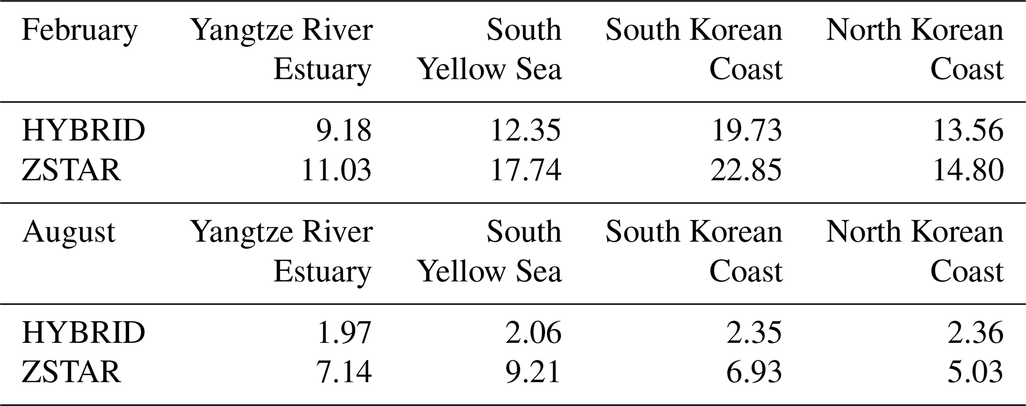
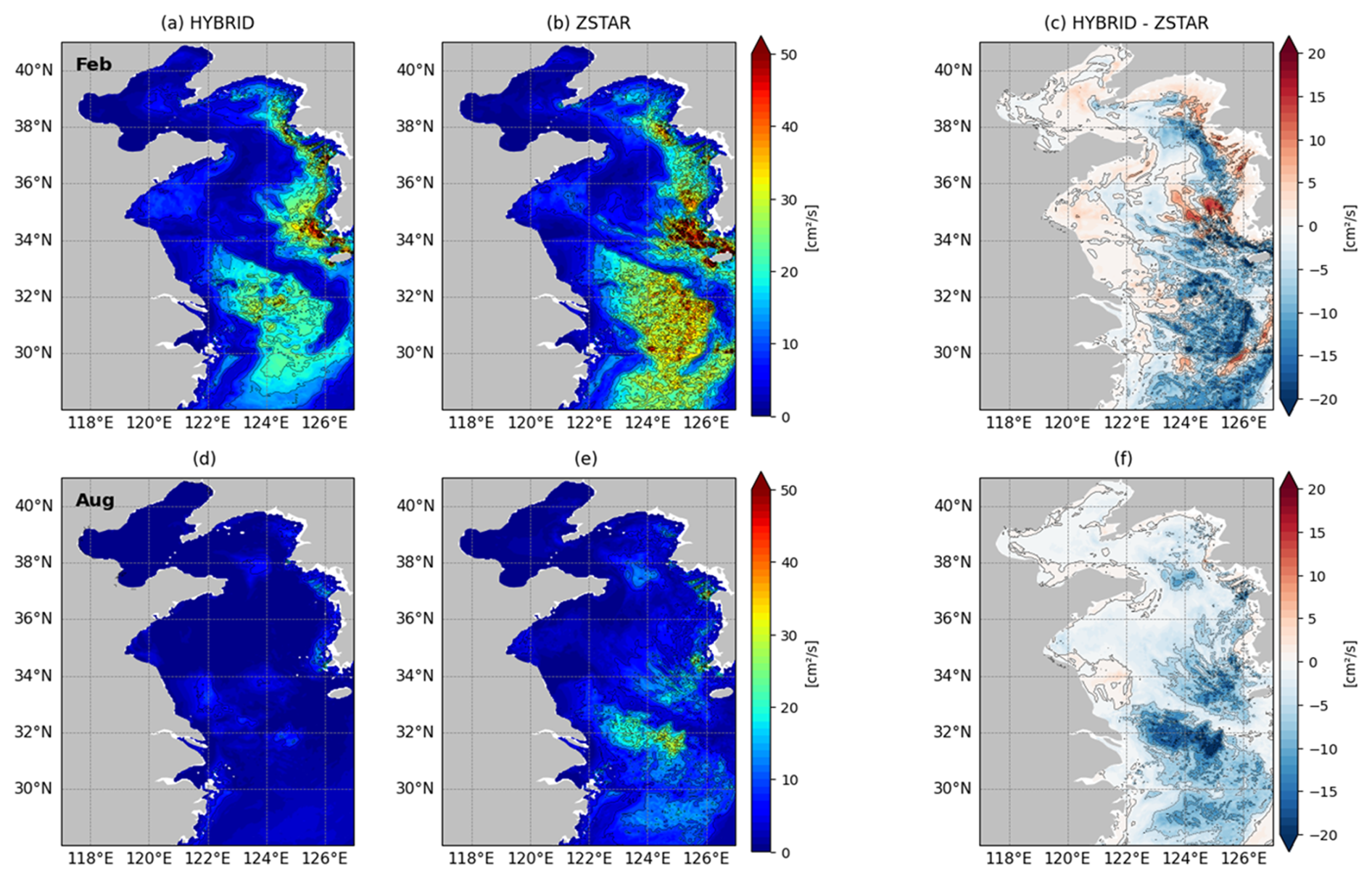
Figure 14 Spatial distribution of depth-averaged shear-driven diapycnal diffusivity (m² s⁻¹) diagnosed by HYBRID and ZSTAR in the Yellow Sea. Panels (a)–(b) and (d)–(e) show the February and August distributions for each configuration, respectively. Panels (c) and (f) present the differences between HYBRID and ZSTAR.

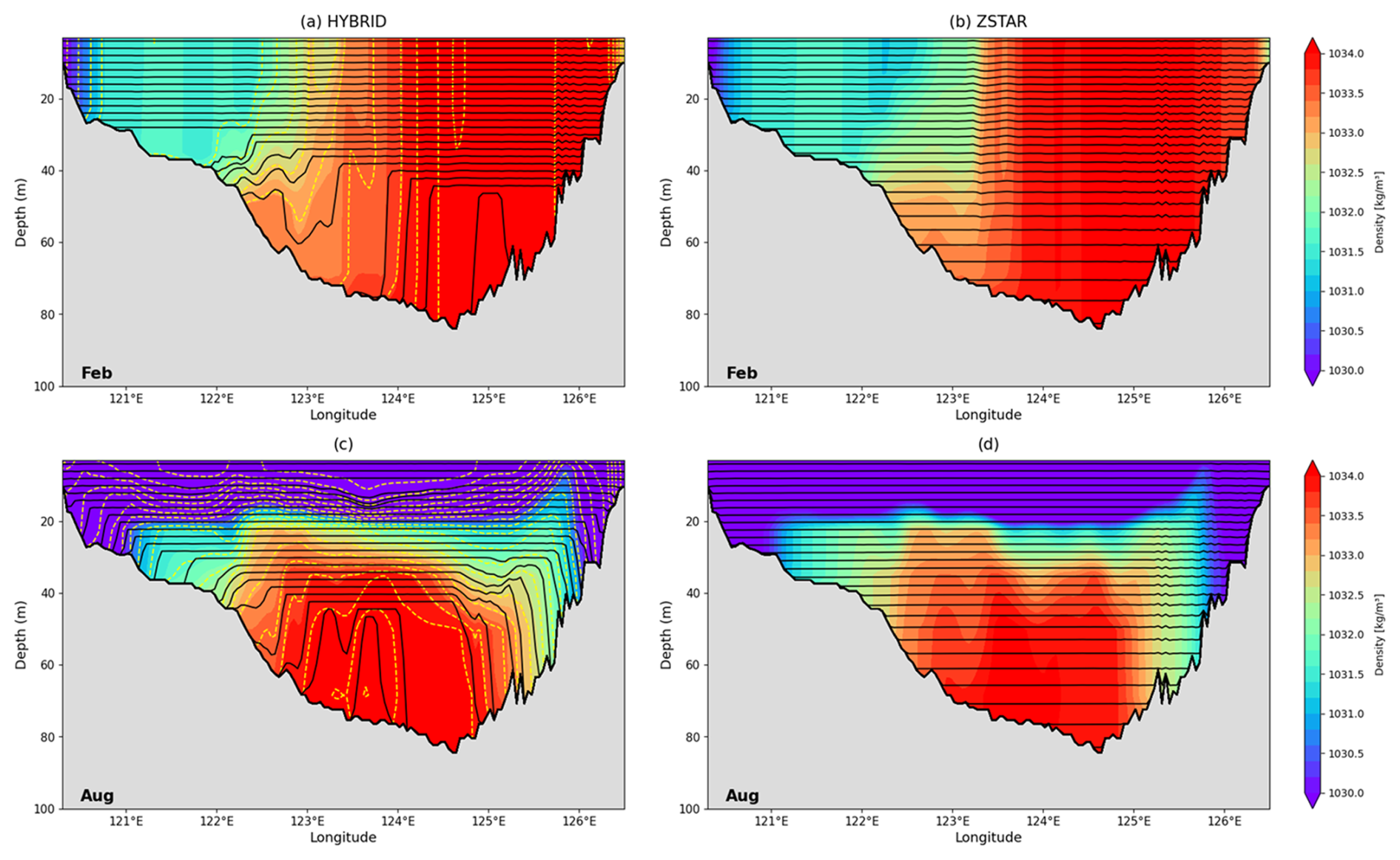
Figure 15 Zonal sections of the model interfaces and density along 36° N in the Yellow Sea for HYBRID and ZSTAR on (a–b) 8 February and (c–d) 8 August. The background color contours represent potential density referenced to 2000 dbar. Black lines denote model layer interfaces and yellow dashed lines indicate target density surfaces used in the HYBRID configuration.

To complement this analysis, Fig. 15 compares the cross sections of the potential density and model interfaces along 36° N in February and August. In winter (Fig. 15a, b), both HYBRID and ZSTAR show weak stratification, but HYBRID aligns more closely with the isopycnals, allowing better resolution of the residual gradients. The improved alignment between the model layer interfaces and isopycnals in HYBRID is not only structural but also dynamically responsive to evolving stratification. As stratification intensified, the model increasingly allocates isopycnal layers to regions with sharp density gradients. This is particularly evident in the 10–20 m depth range and near the bottom, where internal tide signals are previously identified in the density time series (Fig. 11). These locations correspond to zones of active internal wave propagation and energy conversion, and the use of isopycnal coordinates in these layers enables HYBRID to more accurately capture the vertical displacement of isopycnals associated with baroclinic tidal motion. In contrast, ZSTAR maintains a z-coordinate structure throughout, which fails to adapt to density stratification, resulting in increased numerical mixing across the density surfaces. The dynamic layering capability of HYBRID enhances its ability to preserve the vertical structure and simulate physically consistent internal tidal energetics, particularly under seasonally stratified conditions.

5 Conclusion

This study clarifies the impact of the vertical coordinate system choice on the simulation of barotropic and baroclinic tides in the Yellow Sea using a high-resolution MOM6 regional configuration. Two vertical coordinate configurations, HYBRID (z^*-isopycnal) and ZSTAR (pure z^*), are compared in terms of their ability to represent tidal dynamics and the associated stratification. The results demonstrate that the HYBRID configuration consistently outperforms ZSTAR in reproducing both barotropic and baroclinic tidal processes. HYBRID not only yields improved agreement with observational datasets in terms of SST, M₂ tidal amplitude, and vertical thermal structure, but also shows enhanced representation of internal tides, particularly during summer, when stratification is strongest. Diagnostics of the baroclinic KE, internal tidal energy flux, barotropic-to-baroclinic conversion rate, and time-resolved density fields indicated that HYBRID more accurately captures the generation, propagation, and vertical structure of internal tides, owing to its improved representation of vertical mixing and enhanced preservation of stratification. This advantage stems from the use of isopycnal coordinates in the ocean interior, which enables the model to preserve sharp thermoclines and suppress spurious vertical mixing.

The implications of these findings extend beyond physical tidal dynamics. As internal tides modulate subsurface mixing and nutrient transport, an improved representation of stratification and internal wave activity in HYBRID may also lead to more realistic simulations when coupled with biogeochemical models. In contrast, the excessive vertical mixing observed in ZSTAR could lead to a degraded performance in representing vertical tracer distributions, ecosystem structure, and carbon cycling. Thus, the choice of a vertical coordinate system is not merely a numerical detail, but a key determinant of model fidelity across both the physical and biogeochemical domains.