The coupled Southern Ocean–Sea ice–Ice shelf Model (SOSIM v1.0): configuration and evaluation

Complex interactions among the ocean, sea ice, and ice shelves in the Southern Ocean are critical for global climate, yet accurately simulating these processes remains challenging in climate models, such as those participating in the Coupled Model Intercomparison Project Phase 6, due to their coarse resolution and incomplete physical components. Therefore, the development of high-resolution circumpolar coupled ocean–sea ice–ice shelf models could improve our understanding of the evolution of the Southern Ocean. In this study, we use the c66m version of the Massachusetts Institute of Technology General Circulation Model, including a sea ice component and an ice shelf component, to configure the coupled Southern Ocean–Sea ice–Ice shelf Model (SOSIM v1.0). Adopting the Refined Topography dataset version 2 for the geometry of seafloor and ice draft, SOSIM features a horizontal resolution of ∼5 km and 70 vertical layers. Forced by the European Centre for Medium-Range Weather Forecasts Reanalysis v5, a long-term integration of SOSIM is run forward from 1979 to 2022, with daily outputs for estimating the oceanic state, sea ice evolution, and basal mass balance of ice shelves. A comprehensive evaluation of the performance of SOSIM has been conducted against multiple observational and reanalysis datasets. Identified biases include an underestimated Antarctic Circumpolar Current transport, an overestimated Antarctic Slope Current, a warm drift in abyssal waters, an exaggerated seasonality of sea ice extent, and an underestimated total ice shelf mass loss. Despite these limitations, SOSIM still captures large-scale hydrographic structures, the annual variability of sea ice, and cross-slope exchanges over shelf seas. Furthermore, SOSIM is set to serve as the dynamical core for the next-generation Southern Ocean Ice Prediction System being developed in China.

1 Introduction

The Southern Ocean is susceptible to rapid climate change due to complex interactions within the coupled ocean–sea ice–ice shelf system (Cavalieri et al., 2003; Martinson, 2012; Talley, 2013; Padman et al., 2018; Cai et al., 2023). The Southern Ocean is generally taken to be south of 60° S or to the northern limit of the Antarctic Circumpolar Current (ACC). Driven by the westerlies, the eastward-flowing ACC is the largest current in the global ocean, with an average transport ranging from ∼134 to ∼173 Sv (1 Sv=10⁶ m³ s⁻¹) through the Drake Passage (Whitworth, 1983; Whitworth and Peterson, 1985; Koenig et al., 2014; Donohue et al., 2016; Xu et al., 2020). In the farther south, the westward-flowing Antarctic Slope Current (ASC) encircles Antarctica and resides on the continental slope (Thompson et al., 2018). Cyclonic subpolar gyres circulate between the ACC and the ASC, including the Weddell Gyre, the Ross Gyre, and the Australian-Antarctic Gyre.

The primary water masses identified in the Southern Ocean include Antarctic Surface Water (AASW), Shelf Water (SW), Antarctic Bottom Water (AABW), Circumpolar Deep Water (CDW), Antarctic Intermediate Water (AAIW), and Subantarctic Mode Water (SAMW) (Whitworth et al., 1998; Talley, 2013). AASW is the water mass in the upper layer around the Antarctic margins, and it is highly variable due to the atmospheric forcing and sea ice evolution. SW is the water mass in the lower layer over the continental shelf, and its properties are relatively stable due to its isolation from the surface forcing. Formed by dense overflows of SW across the continental slope, AABW is the coldest and densest water mass of the oceans. CDW is formed in the Southern Ocean from a complex mixture of North Atlantic Deep Water, Indian and Pacific deep waters, and modified Antarctic waters. As CDW intrudes onto the continental shelf from the deep ocean, CDW contributes to the formation of modified CDW (MCDW) by mixing with SW (Herraiz-Borreguero et al., 2015; Rintoul et al., 2016; Liu et al., 2017; Liu et al., 2022). AAIW is produced by the subduction between the Polar Front (PF) and the Subantarctic Front (SAF), and SAMW is produced by the subduction between the SAF and the Subtropical Front (STF).

In contrast to the ocean at lower latitudes, sea ice persists in the Southern Ocean, with a pronounced seasonal cycle in the extent and thickness (Hobbs et al., 2016; Meredith and Brandon, 2017). The seasonal cycle of freezing/melting and drifting of sea ice is largely determined by the seasonality of the atmospheric forcing. Covered by sea ice, the ocean is prevented from intensive heat loss to the atmosphere in the austral winter, yet the leads and polynyas occurring within sea ice expanses still expose the ocean to the harsh atmosphere. Because of the intensive brine rejection within polynyas, polynyas are often closely associated with the formation of dense SW, which is the precursor of AABW (Gordon et al., 2009).

Ice shelves are the marine-terminating glaciers of the Antarctic Ice Sheet, and Ice Shelf Water (ISW) is formed as a mixture of the ice shelf melting water and surrounding water masses in the sub-ice-shelf cavities. The mass loss of the Antarctic Ice Sheet to the Southern Ocean is mainly induced by the basal melting and calving of ice shelves (Rignot et al., 2013). Meanwhile, the Antarctic Ice Sheet is also buttressed by ice shelves (Gagliardini et al., 2010; Pritchard et al., 2012; Joughin et al., 2014), and thereby changes in the thickness and extent of ice shelves potentially influence the sea level rise (Zwally et al., 2005; Shepherd et al., 2018). While the basal melting and calving of ice shelves are strongly impacted by the oceanic forcing (Rignot and Jacobs, 2002; Rignot et al., 2008; Holland et al., 2020), the heat and freshwater fluxes at the interface between the ocean and ice shelves are also expected to play an important role in the Southern Ocean (Adusumilli et al., 2020). The latest Coupled Model Intercomparison Project Phase 6 (CMIP6) provides multiple ensemble members of the coupled ocean–sea ice models (Eyring et al., 2016), yet CMIP6 does not include the ice-shelf models, with relatively larger biases in the simulated Southern Ocean. Considering the complexity of the Southern Ocean, the development of high-resolution coupled circumpolar ocean–sea ice–ice shelf models has broad applications.

Modelling of the interactions between the Southern Ocean, sea ice, and ice shelves can provide insights into the complex processes in the Southern Ocean (Busalacchi, 2004; Noerdlinger and Brower, 2007; Shepherd et al., 2010; Rignot et al., 2013; Deconto and Pollard, 2016). An increasing number of Circumpolar coupled Ocean–Sea ice–Ice shelf Models (COSIMs) have been developed for the investigations focused on the Southern Ocean and shelf seas around Antarctic margins.

An early development was the pioneering COSIM of Timmermann et al. (2002), which was based on a dynamic-thermodynamic sea ice model and an S-coordinate (terrain-following) primitive equation model. The ice shelf model is developed from the modified sea ice model. To represent an ice shelf with constant thickness, Timmermann et al. (2002) set the ice concentration to 100 % at ice shelf grids, and the ice velocity was set to 0. Timmermann et al. (2002) also noted that the zero-layer approach for heat conduction of the sea ice model may not be fully applicable to represent the thermal inertia of an ice shelf. Timmermann et al. (2012) further introduced the ice shelf thermodynamics into the global Finite Element Sea–ice Ocean Model (FESOM). The FESOM consists of a hydrostatic primitive-equation finite element ocean model and a dynamic-thermodynamic finite element sea ice model. Timmermann et al. (2012) augmented the FESOM with an ice shelf model by using a three-equation system to simulate the boundary layer temperature and salinity at the ice shelf–ocean interface.

Further advancements were achieved by incorporating ice shelves into other ocean modelling frameworks. By following the ice shelf modelling method in Losch (2008), Kusahara et al. (2010) incorporated an ice shelf component into a coupled ocean–sea ice model (Hasumi, 2006), and the one-layer sea ice model employs a no-heat capacity layer for snow (Bitz and Lipscomb, 1999). Based on this coupled ocean–sea ice–ice shelf model, Kusahara and Hasumi (2013) developed a circumpolar configuration with a northern boundary at about 35° S in the Southern Ocean. Using the Massachusetts Institute of Technology General Circulation Model (MITgcm) (Marshall et al., 1997), Holland et al. (2014) developed a regional coupled ocean–sea ice–ice shelf model covering the domain south of 30° S. The MITgcm contains a dynamic and thermodynamic active sea ice model and a static and thermodynamic active ice shelf model (Losch, 2008). Compared to the employment of sigma grids in the sub-ice-shelf cavities in the FESOM, the ice shelf model in the MITgcm employs a z coordinate in the vertical to simulate the ice shelves. Dinniman et al. (2015, 2020) used the Regional Ocean Modeling System (ROMS) to develop a circum-Antarctic ocean–sea ice–ice shelf model. A two-layer dynamic sea ice model is contained in ROMS, and ice shelves are prescribed as static floating ice by an ice shelf model. The ice shelf model in ROMS can simulate the mechanical and thermodynamic effects of ice shelves on the ocean in the sub-ice-shelf cavities, and the heat and freshwater fluxes at the ice shelf–ocean interface are dependent on the friction velocity.

Recent advances are exemplified by the development of global model configurations, coordinated model intercomparisons, and high-resolution studies. Schodlok et al. (2016) developed a global coupled ocean–sea ice–ice shelf model based on the Estimating the Circulation and Climate of the Ocean Phase II (ECCO2) (Menemenlis et al., 2008) that is configured with the MITgcm. ECCO2 has already included the sea ice model, and Schodlok et al. (2016) further introduced the representation of Antarctic ice shelf cavities into ECCO2. Naughten et al. (2018) conducted an Intercomparison between two coupled ocean–sea ice–ice shelf models: the FESOM 1.4 and the ROMS coupled to Community Ice CodE with ice shelf (MetROMS-ice shelf). The MetROMS-ice shelf consists of the ROMS, the sea-ice model Community Ice CodE, and an ice shelf model, with a circumpolar Antarctic domain, while the FESOM 1.4 includes a finite element sea ice model and an ice shelf model with a steady state for ice shelf thickness. Recently, Dinh et al. (2024) presented a coupled ocean–sea ice–ice shelf model based on the MITgcm, the Southern Ocean model (SOhi). With an uneven horizontal resolution of (from $\mathrm{1}/\mathrm{24}$° at 85.5° S to $\mathrm{1}/\mathrm{12}$° at ∼35° S) and a very high vertical resolution (225 vertical levels), the SOhi captures the critical role of high resolution and accurate bathymetry in promoting warm water intrusion onto the Antarctic continental shelf.

Previous COSIMs are valuable in improving our understanding of climate change, yet the COSIMs also have difficulties in compromising between computational cost and resolving mesoscale processes. Most COSIMs are limited by the coarse resolution and the accuracy of topography. Mesoscale processes have already been highlighted in the Southern Ocean and around the Antarctic margins, yet it is still a challenge for COSIMs to capture mesoscale eddies in the Southern Ocean and mesoscale cross-slope exchanges. The first baroclinic Rossby radius of deformation ranges from ∼30 km at 40° S to less than 5 km over the Antarctic continent shelf (Chelton et al., 1998), while the horizontal resolutions of previous COSIMs generally range from ∼100 to ∼10 km in the Southern Ocean. Previous COSIMs intend to increase the horizontal resolution around the Antarctic margin, yet the horizontal resolutions of most COSIMs are still coarser than 5 km along the Antarctic continental slope (Timmermann et al., 2002; Dinniman et al., 2015).

Cross-slope warm water intrusions from the deep ocean to the continental shelf play an important role in the maintenance of the high basal melting rate of ice shelves in West Antarctica. Naughten et al. (2018) found that both MetROMS-ice shelf and FESOM 1.4 struggled to reproduce the high melting rate of ice shelves in the Amundsen and Bellingshausen seas, probably due to the missing cross-slope warm deep water intrusions in West Antarctica. Meanwhile, the topography and the geometry of ice cavities are expected to be more accurately represented by high resolution, with an improvement in the simulated dynamic influences of topography on the oceanic currents and the basal mass balance of ice shelves. By introducing two singular points in the Southern Hemisphere, Kusahara et al. (2011) and Hirano et al. (2023) increased the horizontal resolution to 3–4 km in a focal region, yet the resolution of the circumpolar Southern Ocean is still relatively coarse. Based on the ROMS, Dinniman et al. (2015) configured a high-resolution circumpolar coupled ocean–sea ice–ice shelf model, with a horizontal resolution refined to 10 km around the entire Antarctica, and Dinniman et al. (2020) further refined the horizontal resolution from 10 to 5 km. The ROMS employs a sigma (terrain-following) coordinate that provides a convenient way of resolving the ice shelf–ocean boundary layer. However, the topography in sigma coordinate models generally needs to be smoothed to avoid spurious velocity induced by the numerical representation of pressure gradient terms, especially near the ice shelf edges (Mack et al., 2017; Mack et al., 2019). The z-coordinate models suffer from representing bottom and ice draft boundary layers due to spurious diabatic mixing, yet the topography can be more accurately introduced by the z-coordinate models without the concern of pressure gradient errors. Therefore, the development of a high-resolution circumpolar coupled ocean–sea ice–ice shelf model with the z-coordinate also provides insights into our understanding of cross-slope and cross-ice-shelf-front exchanges.

To refine the relatively coarse resolutions and include a high-resolution topography data set, by employing the MITgcm with z coordinate, we configured a high-resolution circumpolar coupled ocean–sea ice–ice shelf model to simulate the complex evolution of the Southern Ocean. Our efforts in developing this circumpolar coupled ocean–sea ice–ice shelf model aim in three directions: (i) incorporating interactive ocean, sea ice, and ice shelf components; (ii) employing a high resolution to get a good representation of the topography, ice cavity geometry, and mesoscale eddies in the Southern Ocean; (iii) conducting a comprehensive model evaluation to establish the confidence for its application in future studies. In addition, this model serves the development of the next version of the Southern Ocean Ice Prediction System in China (Zhao et al., 2024). The paper is organized as follows. Section 2 provides descriptions of the model implementation and the observational data sets used for evaluating the simulations. We present a comprehensive evaluation of the model performance in Sect. 3. Section 4 summarizes possible reasons for discrepancies and provides a discussion of the advantages and modelling improvements in the future. Section 5 summarizes our conclusion.

2 Model description

2.1 General components and packages

Based on the MITgcm c66m version, we configured the coupled Southern Ocean–Sea ice–Ice shelf Model version 1.0 (SOSIM v1.0). In the MITgcm, the ocean, sea ice, and ice shelf components share the same horizontal grid layout (the Arakawa C-grid). The ocean component is based on the primitive equations with the Boussinesq approximation and hydrostatic assumption (Marshall et al., 1997). The sea ice component is included to simulate the freeze-thaw cycles of dynamic and thermodynamically active sea ice (Zhang and Hibler, 1997; Losch et al., 2010), and the ice shelf component is introduced to represent static and thermodynamically active ice shelves (Losch, 2008). By using the external forcing package, the heat, freshwater, and momentum fluxes at the atmosphere–ocean, ice–atmosphere, and ice–ocean interfaces are calculated from the atmospheric and oceanic states. In addition, the package of the open boundary condition is introduced to apply the dynamic and thermodynamic forcing at the vertical oceanic open boundaries of this regional model. Since this study does not develop any new package for SOSIM, we focus on the specific configurations of SOSIM below. Indeed, SOSIM is built on the backbone of the southern face of the ECCO2 (Menemenlis et al., 2008), featuring a finer spatial resolution and the inclusion of ice shelves.

2.2 Model domain and spatial discretization

The model domain is placed on a square region centered on the South Pole (Fig. 1a). For such a square box, the latitude covers the Southern Ocean from the South Pole to 35.7° S, with the latitude of the northern boundary ranging from ∼35.7° S at corners to ∼50.2° S at the inscribed circle (Fig. 1b). The longitude range is from 180° W to 180° E, placing the join in the Southern Pacific Ocean.

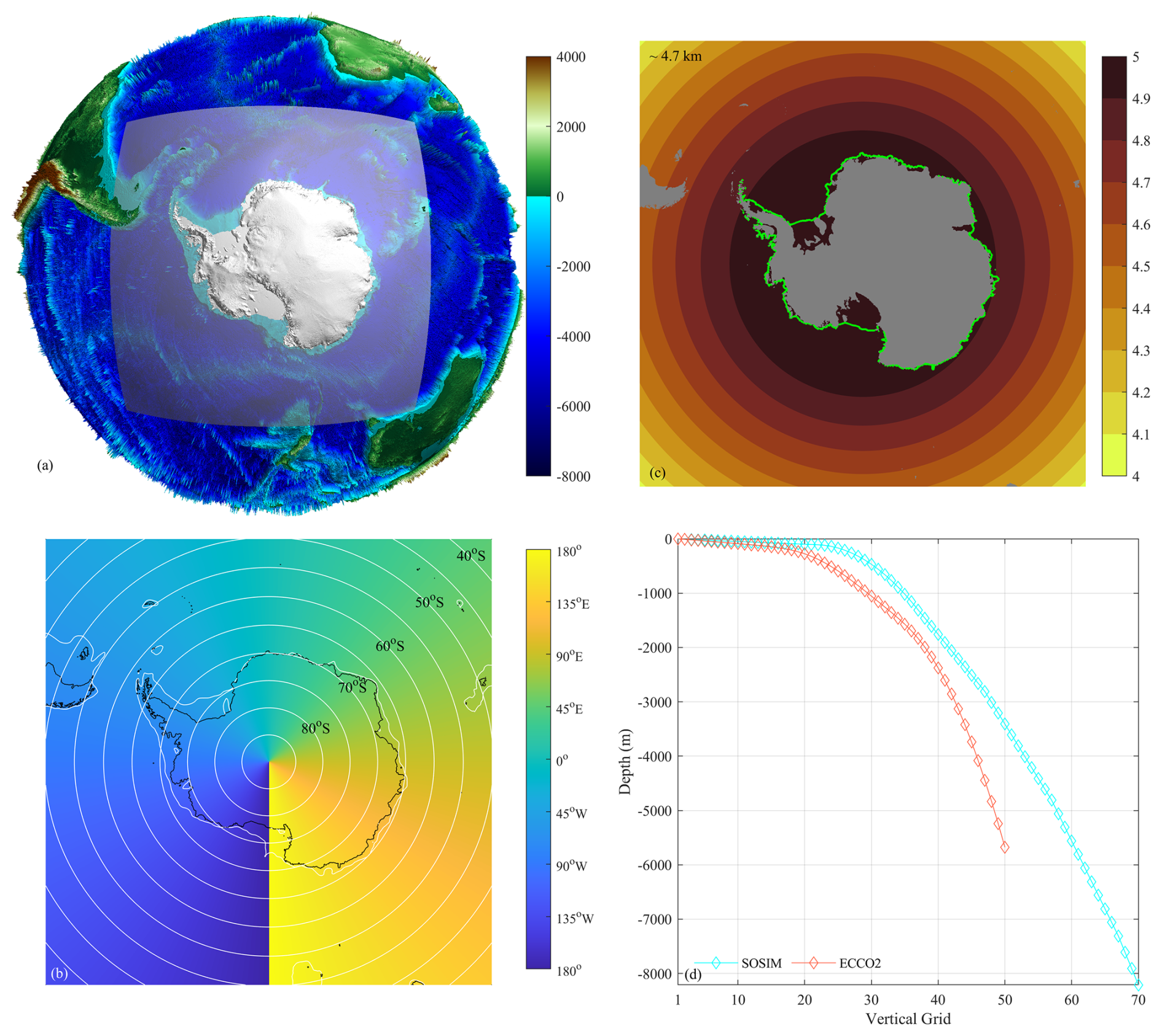
Figure 1 The domain and spatial discretization of SOSIM. (a) A plan view of the model domain in a three-dimensional Earth. The color shading shows the elevation (m) of the solid earth in the Refined Topography data set 2 (RTopo-2) (Schaffer et al., 2016), and the white semi-transparent region shows the domain of SOSIM. (b) The geographic coordinates of the SOSIM grids. The color shading denotes the longitudes, and the white lines denote the latitudes. (c) The horizontal resolution (km) of wet bins in the orthogonal curvilinear mesh. The green line denotes the coastline and the front of the ice shelves. (d) The distribution of the vertical levels. The cyan line denotes the vertical grids of SOSIM, and the orange line denotes the vertical grids of ECCO2.

To avoid the influences of polar singularity at higher latitudes, the horizontal grids employ an orthogonal curvilinear projection, with 1800×1800 horizontal Arakawa C grids. The grid spacing ranges from ∼4 km at the northern boundary to ∼5 km around the coast of Antarctica (Fig. 1c), with an average spacing of ∼4.7 km. Such a high horizontal resolution allows SOSIM to resolve mesoscale eddies in the deep Southern Ocean, where the first baroclinic Rossby deformation radius is ∼20 km (Chelton et al., 1998). Over the shelf seas around Antarctica, this horizontal mesh may be only eddy-permitting. The vertical discretization of SOSIM has 70 levels, ranging from a 5 m interval in the upper layers to a 300 m interval at the deeper layers (Fig. 1d), with partial cells to improve the representation of the bedrock and the ice draft of ice shelves (Adcroft et al., 1997). Compared to the 50 vertical layers in the ECCO2, the vertical discretization in SOSIM increases more smoothly in the upper 1000 m layer and extends to the abyssal layer at 8000 m depth. In SOSIM, the minimum thickness of a partial cell is 30 % of the full cell thickness, or 50 m, whichever is greater.

2.3 Model topography and regional division

The topography datasets in SOSIM are derived from the RTopo-2 (Schaffer et al., 2016), which is a consistent global map that is placed on a spherical grid with 30 arcsec grid spacing, including the bedrock and ice draft topographies. In SOSIM, the bedrock includes the region beneath the Antarctic Ice Sheet (Fig. 2a), and the Antarctic Ice Sheet is represented by grounded glaciers and free-floating ice shelves (Fig. 2b), with sub-ice-shelf cavities located where the ice draft does not extend to the seafloor (Fig. 2c). Accordingly, the water column thickness over the wet bins includes the sub-ice-shelf cavities, shelf seas, and open oceans (Fig. 2d).

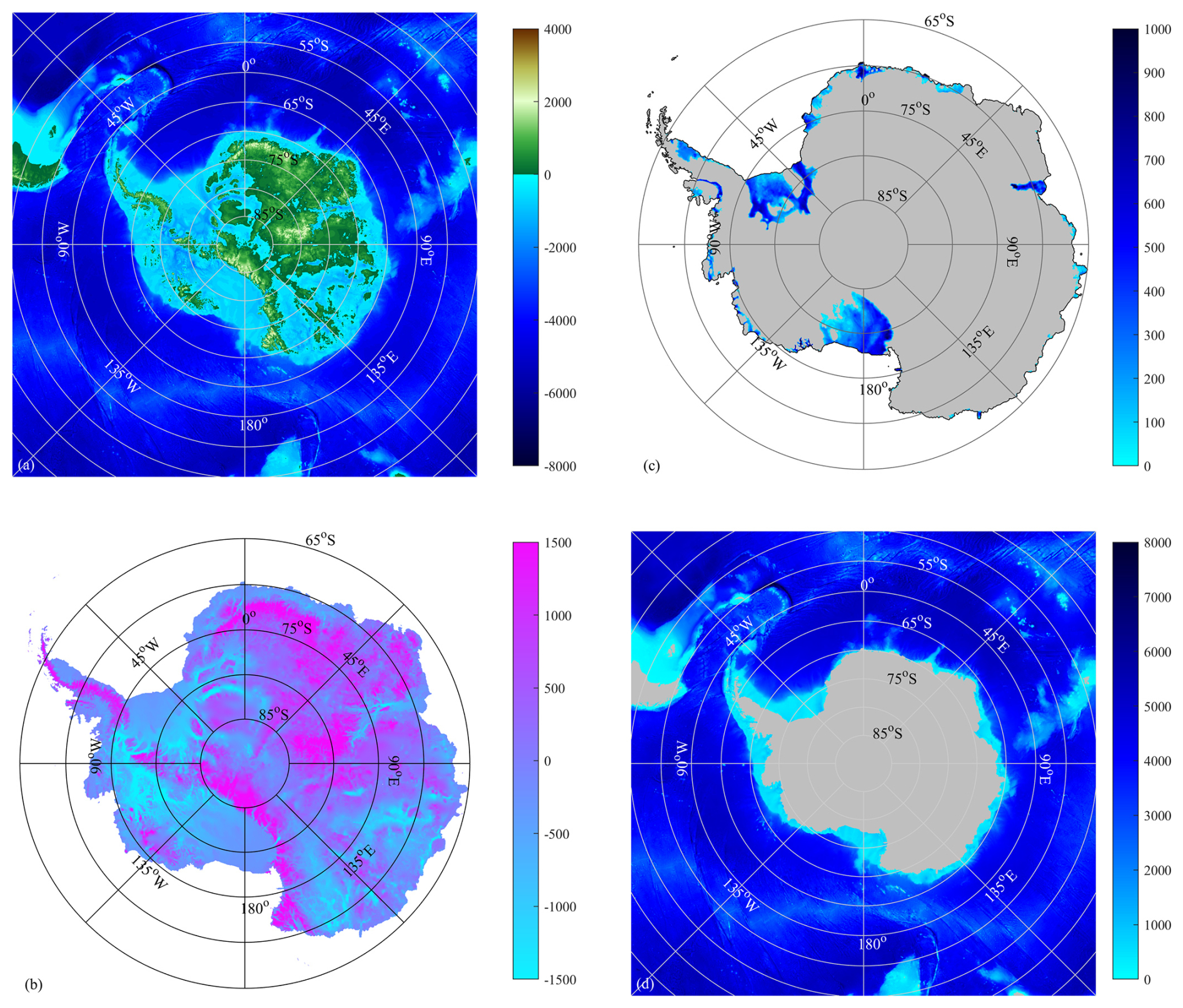
Figure 2 The topography of SOSIM derived from the RTopo-2 dataset. (a) The depth (m) of the bedrock. (b) The ice draft (m) of the Antarctic Ice Sheet. (c) The water column thickness (m) in sub-ice-shelf cavities. (d) The water column thickness (m) of the shelf seas and open oceans. The grey region denotes dry bins.

More efforts are necessary to create the geometry datasets of the bedrock and sub-ice-shelf cavities for SOSIM. The topography of SOSIM is obtained by remapping the RTopo-2 onto the model mesh, with the nearest neighbor interpolation. This gross interpolation would introduce some artifacts into the model topography, especially in the coastal region and islands around the Antarctic Peninsula. Therefore, the coastal region and archipelagos need to be eye-inspected and hand-edited to remove non-advective cells that are isolated from the open ocean. In addition, the inland lakes over South America and the subglacier lakes beneath the Antarctic Ice Sheet also need to be eliminated from the bedrock dataset manually (see Sect. S1 in the Supplement in detail).

2.4 Initial conditions

Initial conditions of the potential temperature (θ) and salinity (S) are derived from the climatology World Ocean Atlas 2018 (WOA18) (Locarnini et al., 2018; Zweng et al., 2018). The “decav” product (an average of all available data) of WOA18 provides objectively analyzed climatological mean fields on a 0.25°×0.25° spherical grid, and thereby we interpolate the WOA18 dataset from its original grids to the mesh of SOSIM (Fig. 3a and b). Since the maximum depth of the climatological mean fields of WOA18 is 5500 m, the deeper layers (>5500 m) of the initial conditions of θ and S in SOSIM are obtained by extrapolating downward, with all wet grid cells located below 5500 m depth set to the values of the deepest valid level from the WOA18 climatology for that same water column. There are no data in the sub-ice-shelf cavities in the WOA18, and θ and S in the sub-ice-shelf cavities are set as −1.96 °C and 34.5 psu for the initial conditions of SOSIM, respectively. The neutral density (γⁿ) calculated based on the initial condition of θ and S shows the initial state of the stratification (Fig. 3c).

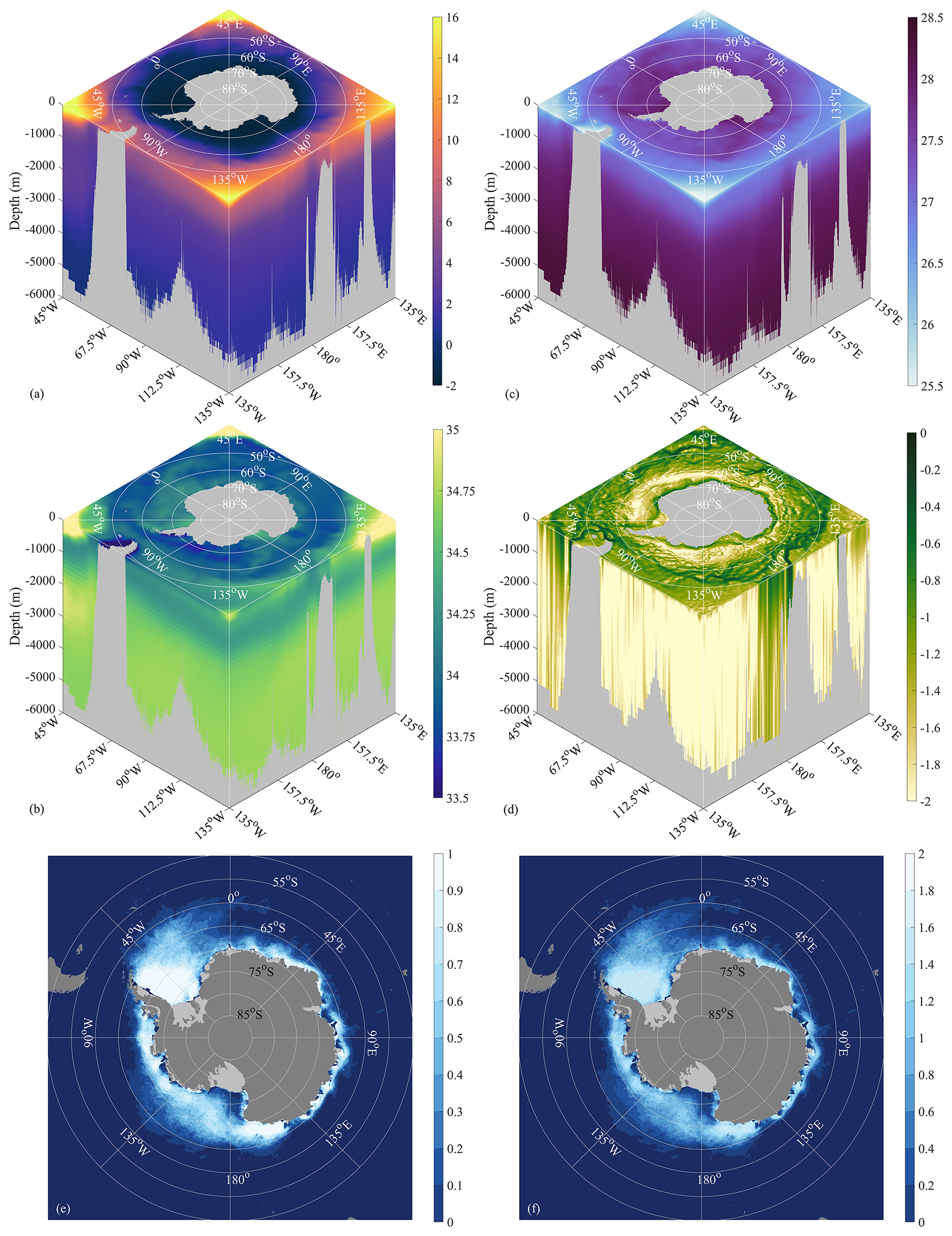
Figure 3 The initial conditions derived from WOA18, ECCO2, and satellite observations. (a) The initial condition of θ (°C) derived from WOA18. (b) The initial condition of S (psu) derived from WOA18. (c) γⁿ (kg m⁻³) calculated based on the initial conditions of θ and S. (d) The logarithmic magnitude (${\log }_{\mathrm{10}}\left(\right|\mathit{u}\left|\right)$) of the initial condition of the velocity fields (m s⁻¹) derived from ECCO2. (e) The initial condition of the SIC derived from the UB. (f) The initial condition of the SIT (m) derived from the UB.

Initial conditions of the velocity fields (u) are derived from the climatology mean of ECCO2 (Fig. 3d). The grid mesh in ECCO2 is placed on a cube sphere, with a horizontal resolution of ∼18 km (Menemenlis et al., 2008). Since ECCO2 does not include the ice shelf component, the initial velocity fields in the sub-ice-shelf cavities are simply set to 0 when we interpolate the ECCO2 velocity from its cube sphere grids to the mesh of SOSIM. Note that the velocity in the geographic coordinate from ECCO2 needs to be rotated to the orthogonal curvilinear coordinate of SOSIM.

Initial conditions of the sea ice are derived from satellite observations (the Advanced Microwave Scanning Radiometer for EOS, AMSR-E; Advanced Microwave Scanning Radiometer 2, AMSR2) provided by the Institute of Environmental Physics, University of Bremen (UB) (Spreen et al., 2008; Huntemann et al., 2014). The grid mesh of the satellite-observed sea ice is placed on a polar coordinate, with a horizontal resolution of ∼6.5 km. Since SOSIM was initialized on 1 January, the daily climatology of Sea Ice Concentration (SIC) and Sea Ice Thickness (SIT) on 1 January from the UB is interpolated from the polar coordinate to the mesh of SOSIM (Fig. 3e and f).

2.5 External forcing

The external forcing of SOSIM includes the surface atmospheric forcing, the oceanic open boundary forcing, and the runoff. SOSIM is forced with the European Centre for Medium-Range Weather Forecasts Reanalysis v5 (ERA5) atmospheric product (Hersbach et al., 2020), with a temporal resolution of 1 h and a horizontal resolution of ∼31 km. Such a high spatial and temporal resolution of ERA5 is useful for the simulation of the high-frequency wind power input into the Southern Ocean (Wu et al., 2020), and it could also improve the representation of coastal polynyas (Stössel et al., 2011; Zhang et al., 2015). The atmospheric forcing dataset from ERA5 includes 10 m winds, 2 m air temperature, 2 m specific humidity, precipitation, downward shortwave radiation, and downward longwave radiation. The temporal coverage of ERA5 extends from January 1940 to near present day, with satellite observations assimilated from 1979 onward, and SOSIM uses 1979–2022 inclusive for the integration in the current version.

Akin to the initial conditions, the oceanic open boundary conditions of SOSIM are also derived from WOA18 and ECCO2 (Fig. 4a–d). The open boundary conditions of θ and S are derived from the monthly climatology of WOA18 (Fig. 4a and b), and the velocity is derived from ECCO2 (Fig. 4d). Since the monthly climatology of WOA18 only provides data from 0 to 1500 m depth, the data below 1500 m depth on the open boundary is fixed as the annual climatology of WOA18. γⁿ, calculated based on the open boundary conditions of θ and S, shows the state of the stratification on the north boundary (Fig. 4c). The open boundary conditions of the velocity denote the velocity perpendicular to the northern boundary. Since the northern boundary is not along a fixed latitude (the black line in Fig. 4e), and the rotation of the geographic velocity in ECCO2 to the curvilinear coordinate of SOSIM is still necessary to calculate the velocity perpendicular to the northern boundary. The northern boundary is located sufficiently north of the maximum sea ice extent, and thereby there is no need to prescribe the open boundary conditions for sea ice.

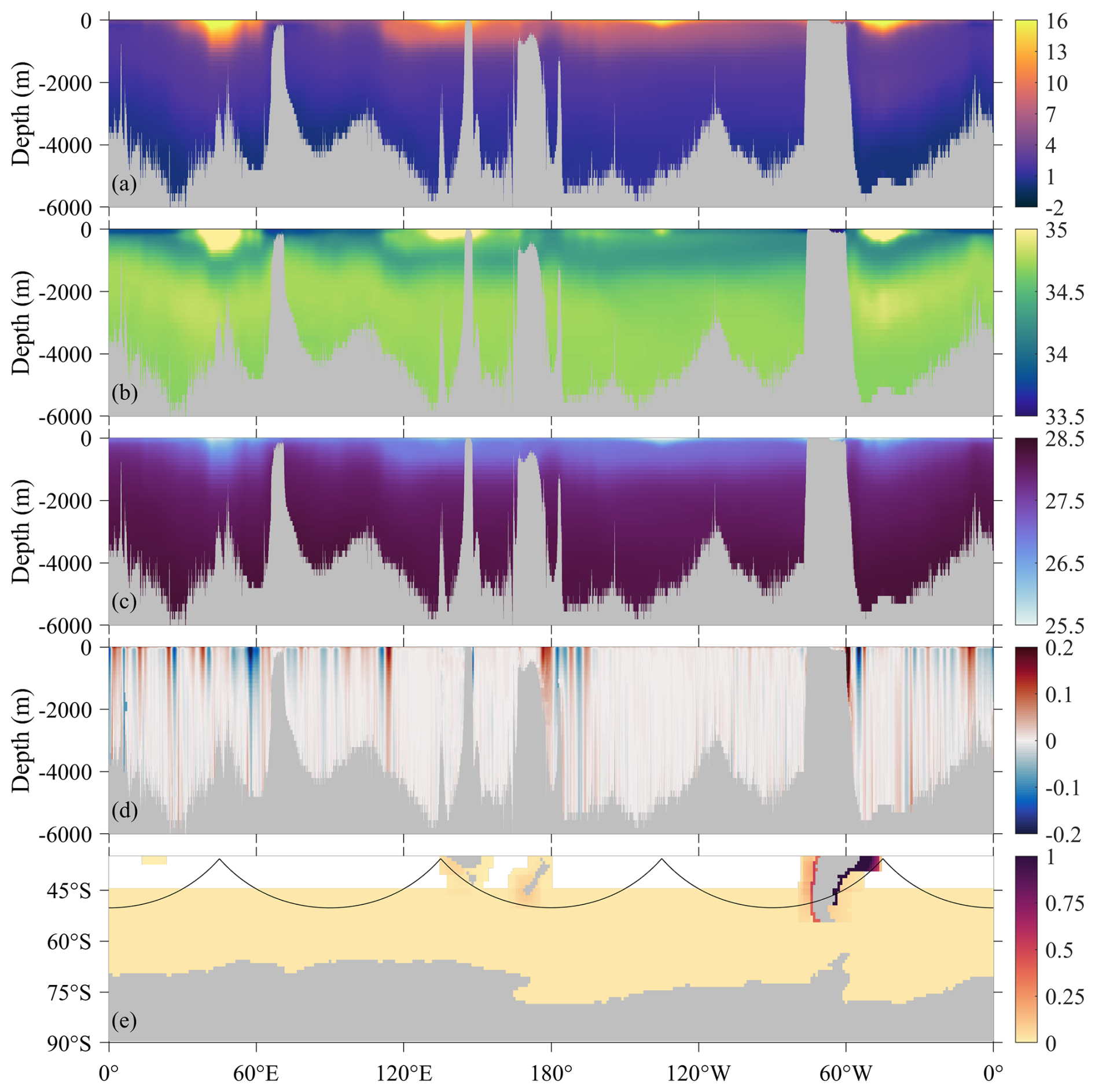
Figure 4 The annual mean of the open boundary conditions and river runoff forcing. Note that the oceanic open boundary conditions in SOSIM are monthly climatology. (a) The open boundary condition of θ (°C) on the northern boundary. (b) As in (a), but for S (psu). (c) γⁿ (kg m⁻³) calculated based on the open boundary conditions of θ and S. (d) As in (a), but for the velocity (m s⁻¹) perpendicular to the northern boundary. (e) The river runoff (m yr⁻¹) employed in SOSIM, with modifications based on the dataset from the Global Runoff Data Centre. The black line shows the position of the open boundary of SOSIM on the Miller Projection.

In ECCO2, the melting and calving of ice shelves around Antarctica are represented by the forcing of glacier runoff derived from the Global Runoff Data Centre, with a fixed value along the coastline around Antarctica. The melting of ice shelves injects freshwater locally, yet the calving of ice shelves and melting of icebergs can discharge meltwater into the ocean farther offshore (Silva et al., 2006; Tournadre et al., 2012; Merino et al., 2016). SOSIM also employed the same glacier runoff dataset as the ECCO2, yet two modifications are configured to better represent the glacier runoff. First, Rignot et al. (2013) found that the basal melting rate (1325 Gt yr⁻¹) of ice shelves around Antarctica is even relatively larger than the calving rate (1089 Gt yr⁻¹). Since SOSIM can simulate the melting of ice shelves directly, the forcing of the glacier runoff is simply halved to only represent the calving of ice shelves and the melting of icebergs. Second, considering that the melting of icebergs occurs along with the northward transport of icebergs, the forcing of glacier runoff has also been uniformly spread farther north between the ice shelf edge and 45° S rather than being constrained within the coastal bins around Antarctica (Fig. 4e). There is no modification to the river runoff dataset around the northern continents in the Southern Ocean.

2.6 Model parameterizations

In the ocean component, since the horizontal resolution of SOSIM is sufficient to resolve mesoscale eddies, the sub-grid-scale parameterization for mesoscale eddies has not been included. The vector-invariant form of the momentum equations is enabled to reduce spurious numerical dissipation in eddy-resolving simulations, with enhanced accuracy on curvilinear grids. The horizontal friction employs the Smagorinsky scheme, with both harmonic and biharmonic viscosity factors of 0.5. The vertical eddy viscosity is set as a constant background coefficient of $\mathrm{5}\times {\mathrm{10}}^{-\mathrm{4}}$ m² s⁻¹. A quadratic bottom-drag coefficient of $\mathrm{2}\times {\mathrm{10}}^{-\mathrm{3}}$ is applied at the seafloor. A non-linear 3rd order flux limiter scheme is adopted for the advection of traces, and the nonlocal K-Profile Parameterization (KPP) scheme is employed for the treatment of vertical mixing (Large et al., 1994). A background Laplacian diffusivity of $\mathrm{1}\times {\mathrm{10}}^{-\mathrm{5}}$ m² s⁻¹ is adopted for the vertical diffusion of tracers. In MITgcm, the prognostic temperature is potential temperature, and the practical salinity is the prognostic tracer of salt. There is no restoration of the sea surface salinity (SSS) or sea surface temperature (SST). SOSIM adopts the seawater equation of state proposed by Jackett and Mcdougall (1995), which uses the simulated θ and a horizontally constant pressure as input.

The sea ice component adopts the zero-layer thermodynamic model (Hibler, 1980) and a viscous–plastic dynamic solution (Hibler, 1979; Zhang and Hibler, 1997), without thickness categories. The air–ice and water–ice drag coefficients are set as $\mathrm{1.8}\times {\mathrm{10}}^{-\mathrm{3}}$ and $\mathrm{5.6}\times {\mathrm{10}}^{-\mathrm{3}}$, respectively. The sea ice strength adopts a constant coefficient of 2.75×10⁴ N m⁻², corresponding to a relatively strong resistance to deformation. The sea surface freezing point is linearly dependent on the salinity, and the lead closing parameter, which determines the partition between lateral and vertical ice-growth rate, is set as 0.5 m. A salt plume scheme is introduced to represent the subgrid-scale brine rejection parameterization due to sea ice formation (Nguyen et al., 2009).

In the ice shelf component, phase changes of ice shelves are assumed to be in thermodynamic equilibrium (Holland and Jenkins, 1999), and the heat and freshwater fluxes at the ice shelf–ocean interface are related to the local freezing point, which is linearly dependent on both the salinity and pressure. The turbulent tracer exchanges at the ice shelf–ocean interface are chosen to follow a friction velocity-dependent transfer parameterization (Jenkins et al., 2010), with a drag coefficient of $\mathrm{5}\times {\mathrm{10}}^{-\mathrm{4}}$.

The ocean, sea ice, and ice shelf components share an identical time step of 80 s for both the momentum and tracer equations, while a longer time step could be numerically unstable due to the CFL condition. The time-staggered algorithm for the time step scheme, which updates the velocity at half-time steps and tracers/pressure at full steps, is used to improve the numerical stability. Model parameterizations are still under continuous optimization, and more configurations can be found in the model configuration files in detail (disclosed in Code and data availability).

2.7 Compilation, execution, and computational performance

The compilation and execution of SOSIM follow the standard procedure for MITgcm-based experiments. After obtaining the MITgcm source code (as referenced in the Code and data availability), users should first create a dedicated subdirectory (e.g., “SOSIMv1”) within the “verification” directory of MITgcm and copy all SOSIM configuration files into it. Subsequently, a “build” directory needs to be created inside “SOSIMv1”. From within this “build” directory, the model executable file “mitgcmuv” is compiled by calling the MITgcm build script, which processes the configuration set in the adjacent “code” directory. Note that specific compiler options and library paths need to be configured according to the computing environment of the local cluster. Finally, the generated executable “mitgcmuv” should be copied into the “input” directory, where the integration is initiated.

SOSIM was run on the cluster of Hohai University in China. The architecture consists of 48 nodes, with a 2 × 32-core Intel Xeon Gold 6458Q (3.10 GHz) CPU and 256 GB RAM per node. Nodes are connected by an InfiniBand EDR interconnect, with a transfer bandwidth of 100 Gb s⁻¹. Executables were compiled with the Intel Fortran version 17 and the Intel C++ Compiler version 17. On this platform, 1 year integration of SOSIM, with 896 cores, 1280 cores, 1664 cores, and 1920 cores, needs a runtime of ∼48, ∼38.5, ∼30, and ∼28 h, respectively. Considering the computational cost and efficiency, a parallel computation with 1664 cores may be the most economical choice. However, due to the limited computational resources, this study had to use 896 cores for the parallel run of SOSIM, and thereby it took ∼4 months to conduct the long-term integration of SOSIM.

2.8 Model integration

SOSIM starts from a 10 year spin-up under a repeated ERA5 forcing from 1 January 1979 to 31 December 1979, and then runs forward from 1979 to 2022, with the interannual forcing from ERA5. Some previous studies employed the atmospheric forcing in a neutral year (such as 1984 or 2007) to spin up the models (Kiss et al., 2020; Richter et al., 2022). A neutral year is expected to have fewer anomalous representations, with neutral states of some major climate modes. Since this study tends to integrate SOSIM from 1979 onwards, and thereby the spin-up of SOSIM with a neutral year rather than the year 1979 may introduce a shock at the early stage of the real-time forcing period. Therefore, we use the year 1979 to spin up SOSIM, and a similar spin-up strategy has also been employed by Holland et al. (2014).

During the 10 year spin-up, monthly outputs are saved to show if SOSIM roughly reaches a stable state. Thereafter, SOSIM is integrated from 1979 to 2022, and daily outputs are saved for the state estimate of the ocean, the sea ice, and the ice shelf. Such high-frequency outputs allow us to assess the mesoscale processes with transient features.

3 Model evaluation

First, we outline the observational data sets and methods used for the model evaluations. Second, we diagnose whether SOSIM reaches a quasi-equilibrium state. Then, to show SOSIM performance comprehensively, we focus on both the temporal changes and spatial patterns of simulated fields under the interannual atmospheric forcing, the years 1979–2022 inclusive. Therefore, despite the model equilibrium diagnosis during spin-up, our evaluations are mostly based on the model outputs during the interannually forcing period.

We first focus on the ocean estimations, then evaluate the simulated sea ice, and finally analyze the representation of ice shelves. For the assessments of SOSIM in this study, climatological annual mean fields are calculated by taking a time-average over the interannual integration from 1979 to 2022. Climatological monthly mean has also been calculated to estimate the seasonal cycle of SOSIM during the interannually forcing period, and the seasons are defined as the austral summer (December, January, and February), the austral autumn (March, April, and May), the austral winter (June, July, and August), and the austral spring (September, October, and November), respectively.

To quantitatively evaluate the model results in different basins, we introduced a basin-scale regional division in the deep Southern Ocean, including the Southern Atlantic sector (67° W–20° E), the Southern Pacific sector (146° E–67° W), and the Southern Indian sector (20–146° E), respectively (Fig. 5a). Over the shelf seas around Antarctica, a more fine-scale division is introduced to separate eight coastal subregions by following the regional division of Stewart et al. (2018), including the West Antarctic Peninsula (WAP) sector, the Bellingshausen sector, the Amundsen sector, the Ross sector, the East Antarctica sector, the Amery sector, the Maud sector, and the Weddell sector (Fig. 5b). Three transects (blue lines in Fig. 5b) across the continental slope are chosen to show the evaluation of the simulated ASC and the Antarctica Slope Front (ASF).

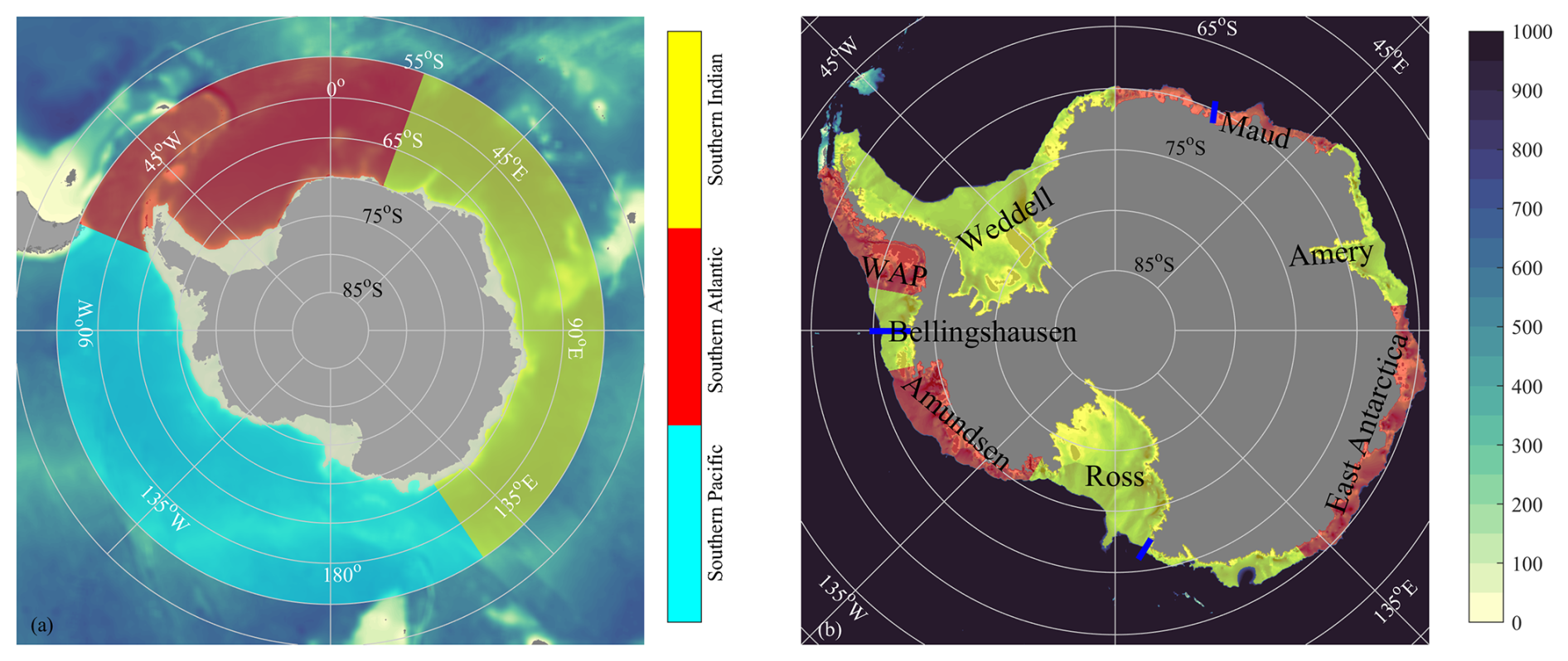
Figure 5 The regional division for model evaluation. (a) The basin-scale regional division and the shelf sea around Antarctica. The red semi-transparent region denotes the Southern Atlantic sector (67° W–20° E), the yellow semi-transparent region denotes the Southern Indian sector (20–146° E), and the cyan semi-transparent region denotes the Southern Pacific sector (146° E–67° W). (b) The alternatively red and yellow regions denote the division of the Antarctic shelf seas (the south of the 700 m isobath) by following Stewart et al. (2018). The blue lines denote three transects across the continental slope, as shown in Figs. 19–21.

For the properties of water masses, we assessed the simulated θ and S in the deep ocean, shelf seas, and the Antarctic continental slope, respectively. For the dynamical characteristics, we evaluate the barotropic streamfunction and the surface kinetic energy, and the dynamic height. We also diagnose the seasonality and interannual variability of the sea ice and the basal melting/freezing rate of ice shelves, respectively. To exclude the nudging influences of the northern open boundary, our evaluations of the oceanic state are conducted within regions to the south of 55° S (noted as the model inner domain below).

To quantify the performance of SOSIM across the ocean, sea ice, and ice shelf components, we present statistical comparisons against observations. Our analysis employs bivariate scatter density plots with marginal distributions to juxtapose simulated and observed values. To provide a quantitative assessment of the model skill, these comparisons are augmented with statistical metrics, including the Spearman correlation coefficient (r), root-mean-square error (RMSE), and mean bias. The probability density function (PDF) is used to elucidate the distributional characteristics of both datasets, annotated with their medians, interquartile ranges, and 95 % data intervals. This multifaceted approach is introduced to evaluate the fidelity of SOSIM in simulating oceanic properties, the sea ice state, and the basal melting/freezing rate of ice shelves. Given the availability of long-term satellite records, we also compare the time series of SIA and SIE with satellite observations.

3.1 Observational datasets for model evaluation

Multiple data sets are used to assess the ability of SOSIM, including objective analysis data sets, in situ hydrography observations, satellite remote sensing data sets, and reanalysis data sets. WOA18 is used to evaluate the simulated θ and S in the deep ocean regions (Locarnini et al., 2018; Zweng et al., 2018). Hydrography observations from the Marine Mammals Exploring the Oceans Pole to Pole (MEOP) consortium are used to evaluate the simulated θ and S over the continental shelf (Roquet et al., 2014; Treasure et al., 2017). Gridded observational data from Yamazaki et al. (2025), denoted as Y2025 hereafter, is introduced to evaluate the simulated ASF over the Antarctic continental slope. A reanalysis dataset of the Southern Ocean State Estimate (SOSE) (Mazloff et al., 2010; Verdy and Mazloff, 2017) is used to evaluate the simulated large-scale circulations and the ASC over the slope. The sea surface dynamic height from the Archiving, Validation and Interpretation of Satellite Oceanographic (AVISO) is used to evaluate the simulated surface geostrophic velocity. Observed sea ice state from the UB (Spreen et al., 2008; Huntemann et al., 2014), the National Snow and Ice Data Center (NSIDC), and the Hokkaido University (HU) (Tamura et al., 2006, 2008) is used to evaluate the simulated sea ice in SOSIM. Satellite observed basal melting/freezing of ice shelves from Rignot et al. (2013) and Adusumilli et al. (2020), denoted as R2013 and A2020 hereafter, is used to compare with the simulated results.

As gridded objective analyses of the World Ocean Database, WOA18 is not only used to construct the initial conditions of θ and S but also for the assessment of the simulated θ and S. Over the continental shelf around Antarctica, instrumented elephant seals provide important in situ oceanographic measurements that are publicly available from MEOP (Roquet et al., 2014; Treasure et al., 2017). Since there are some known biases over the continental shelf in WOA18, we evaluate the SOSIM results over the continental shelf by comparing them with MEOP. To assess the simulated velocity, the surface geostrophic velocity estimated from the AVISO is used to compare with SOSIM. We compare the observed geostrophic Mean Kinetic Energy (MKE) and Eddy Kinetic Energy (EKE) from the AVISO with the SOSIM outputs. The surface geostrophic currents from both AVISO and SOSIM are calculated as follows:

$$\begin{array}{}\text{(1)}& {\displaystyle }{\stackrel{\mathrm{‾}}{u}}_{\mathrm{g}}=-{\displaystyle \frac{g}{f}}{\displaystyle \frac{\partial \stackrel{\mathrm{‾}}{\mathit{\eta }}}{\partial y}}\text{(2)}& {\displaystyle }{\stackrel{\mathrm{‾}}{v}}_{\mathrm{g}}={\displaystyle \frac{g}{f}}{\displaystyle \frac{\partial \stackrel{\mathrm{‾}}{\mathit{\eta }}}{\partial x}}\text{(3)}& {\displaystyle }{u}_{\mathrm{g}}^{\prime }=-{\displaystyle \frac{g}{f}}{\displaystyle \frac{\partial {\mathit{\eta }}^{\prime }}{\partial y}}\text{(4)}& {\displaystyle }{v}_{\mathrm{g}}^{\prime }={\displaystyle \frac{g}{f}}{\displaystyle \frac{\partial {\mathit{\eta }}^{\prime }}{\partial x}}\end{array}$$

where u_g and v_g are the surface geostrophic currents, g=9.8 m s⁻² is the Gravitational constant, f is the planetary vorticity, and η is the sea surface dynamic height. The over bar denotes time mean (1979–2022), and the prime denotes the deviation from the time-mean value. Then, the surface MKE (MKE_surf) and EKE (EKE_surf) is calculated as:

$$\begin{array}{}\text{(5)}& {\displaystyle }{\text{MKE}}_{\text{surf}}={\displaystyle \frac{\mathrm{1}}{\mathrm{2}}}({\stackrel{\mathrm{‾}}{u}}_{\mathrm{g}}^{\mathrm{2}}+{\stackrel{\mathrm{‾}}{v}}_{\mathrm{g}}^{\mathrm{2}})\text{(6)}& {\displaystyle }{\text{EKE}}_{\text{surf}}={\displaystyle \frac{\mathrm{1}}{\mathrm{2}}}(u_{\mathrm{g}}^{\prime \mathrm{2}}+v_{\mathrm{g}}^{\prime \mathrm{2}})\end{array}$$

Direct velocity observations are still limited in the deep ocean in the Southern Ocean, yet a barotropic streamfunction estimated from hydrographic observations (Colin De Verdière and Ollitrault, 2016), denoted as C2016 hereafter, is introduced to qualitatively compare with the simulated transports in SOSIM.

To evaluate the simulated sea ice from SOSIM, we used the SIC and SIT from the UB, the SIC from the NSIDC, and the sea ice production (SIP) from the HU (Tamura et al., 2006, 2008). The UB provides daily SIC and SIT derived from the AMSR-E/AMSR-2 (Spreen et al., 2008; Huntemann et al., 2014). Since the high-resolution sea ice data set from the UB only spans from 2002 to 2019, the SIC from the NSIDC is also adopted for the evaluation of the simulated temporal changes of the sea ice. Daily SIC from the NSIDC is derived from the Special Sensor Microwave/Imager (SSM/I), Scanning Multichannel Microwave Radiometer (SMMR), and Special Sensor Microwave Imager/Sounder (SSMIS), with a horizontal resolution of ∼25 km and a temporal range from 1978 to 2024 (DiGirolamo et al., 2022). Based on the AMSR-E and ERA5 data, the SIP from the institute of low temperature science of the HU is estimated from heat flux during the freezing period (March–October) by assuming that all surface heat loss is used for the SIP (Ohshima et al., 2003), with a horizontal resolution of 6.25 km and a temporal range from 2003 to 2010 (Nakata et al., 2019, 2021). To assess the simulated spatial pattern of basal melting/freezing rates of ice shelves, satellite-observed basal melting rates estimated from radar altimetry (i.e., A2020) are adopted, with a horizontal resolution of 500 m and a temporal average from 2010 to 2018 (Adusumilli et al., 2020). All observational data sets are interpolated onto the SOSIM grid mesh for evaluating the simulated results. The station data sets of θ and S profiles from MEOP are averaged within the nearest bin of the SOSIM grid, and thereby we derive a climatology annual mean of θ and S fields from MEOP over the Antarctic continental shelf.

To maintain a clear focus on the model evaluation, the manuscript presents only the simulated and comparative figures, while the observational data plots are archived in the Supplement.

3.2 Model spin-up and drift

To quantify the spin-up processes of SOSIM, we assessed the evolutions of multiple diagnostics. The domain-integrated Heat Content (HC), Salt Content (SC), Kinetic Energy (KE), Sea Ice Area (SIA), Sea Ice Extent (SIE), and Ice Shelf Melting/Freezing Rate (ISMFR) are calculated as follows:

$$\begin{array}{}\text{(7)}& {\displaystyle }\text{HC}=\int \mathit{\theta }{\mathit{\rho }}_{\mathrm{c}}{C}_p\mathrm{d}V\text{(8)}& {\displaystyle }\text{SC}=\int S{\mathit{\rho }}_{\mathrm{c}}\mathrm{d}V\text{(9)}& {\displaystyle }\text{KE}=\int {\displaystyle \frac{\mathrm{1}}{\mathrm{2}}}(u^{\mathrm{2}}+v^{\mathrm{2}}){\mathit{\rho }}_{\mathrm{c}}\mathrm{d}V\text{(10)}& {\displaystyle }\text{SIA}=\int \text{SIC}\mathrm{d}{S}_{\text{surf}}\text{(11)}& {\displaystyle }\text{SIE}=\int \text{SIext}\mathrm{d}{S}_{\text{surf}}\text{(12)}& {\displaystyle }\text{ISMFR}=\int {\text{SHI}}_{\text{fw}}\mathrm{d}{S}_{\text{shelf}}\end{array}$$

where ρ_c=1026 kg m⁻³ is a constant seawater density adopted in SOSIM, u and v are the horizontal velocity fields, SIext is a Heaviside function worth of 1 for grids where SIC≥0.85 and 0 otherwise, SHI_fw is the freshwater flux at the ice shelf-ocean interface, $\int \cdot \mathrm{d}V$ denotes the volume integral within a selected region, $\int \cdot \mathrm{d}{S}_{\text{surf}}$ denotes the area integral over the surface layer, $\int \cdot \mathrm{d}{S}_{\text{shelf}}$ denotes the area integral over the ice shelf-ocean interface. The linear regressions of these fields are calculated to show the model drift.

Under the repeated atmospheric forcing in 1979, the time series of HC increases in the first 5 year and approaches a quasi-equilibrium in the last 5 years (Fig. 6a). The domain-integrated SC shows a significant decreasing trend throughout the 10 year spin-up, whereas the SC over the continental shelf is almost stable in the last 5 years (Fig. 6b). The domain-integrated KE has a strong increase in the first 2 years and reaches a stable state thereafter, with a very weak decreasing trend in the last 5 years (Fig. 6c), while the KE over the continental shelf approaches a quasi-equilibrium in the second year (Fig. 6c). The winter SIA in SOSIM is smaller than climatology observations from the UB (Fig. 6d), while the seasonality of SIE in SOSIM is larger than observations (Fig. 6e). The drifts of the SIA and SIE are almost negligible in the last 5 years. The simulated mass loss of the ice shelves gradually increases in the first 5 years and reaches quasi-equilibrium in the last 5 years, without any significant trends (Fig. 6f). Compared to the observed values in R2013, the total ice shelf melting rate of SOSIM is relatively smaller. It is worth noting that SOSIM v1.0 does not include tides, yet the tidal contribution to the melting rate of ice shelves cannot be neglected (Padman et al., 2018). For example, the tidal contribution to the basal melting of the Amery Ice Shelf can be up to 69 % at a borehole station (Liu et al., 2023). Therefore, it is expected that the mass loss of ice shelves in SOSIM is smaller than observations (Fig. 6f).

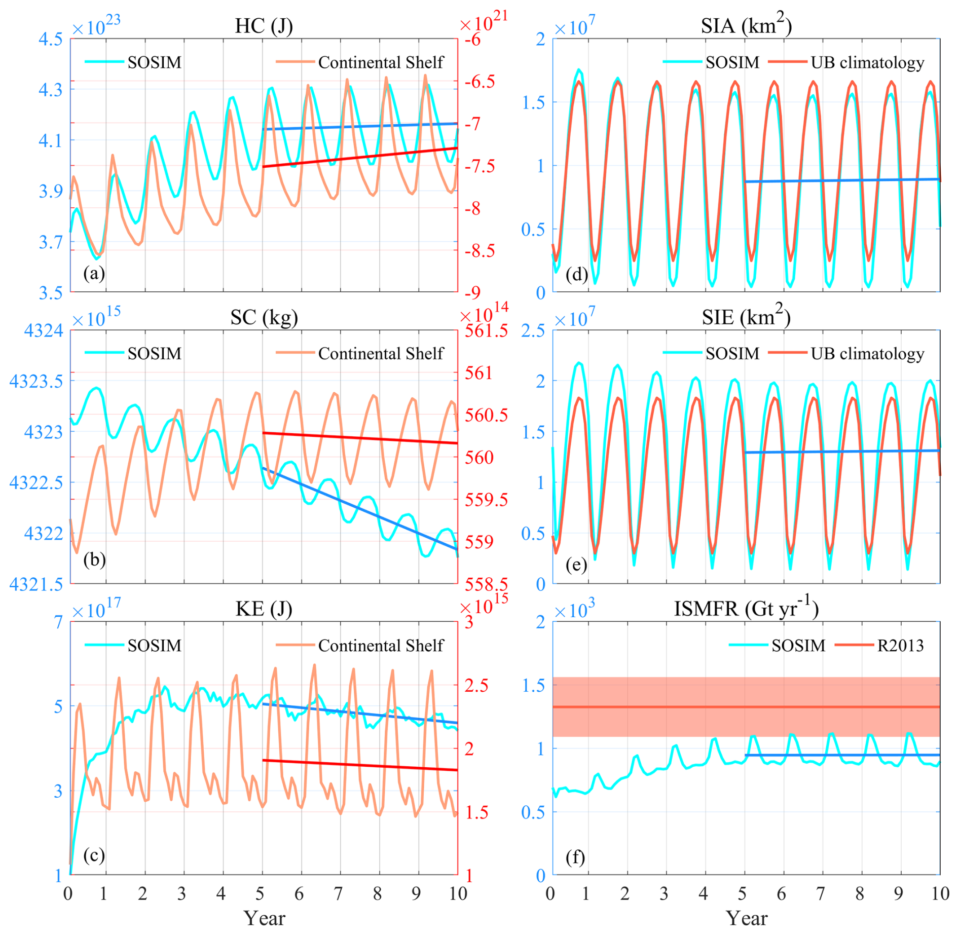
Figure 6 Time series for the assessments of the model spin-up. (a) The cyan line is the time series of the inner domain-integrated HC, and the orange line denotes the time series of HC integrated over the continental shelf (the alternatively red and yellow regions in Fig. 5b). The blue and red lines denote the linear regressions of the cyan and orange lines based on the monthly outs in the last 5 years, respectively. (b, c) As in (a), but for the SC and KE. (d) The cyan line is the time series of the domain-integrated SIA, and the red line denotes the monthly climatology of the satellite-observed SIA provided by the UB. (e) As in (d), but for the SIE. (f) The cyan line is the time series of the domain-integrated ISMFR, and the red line denotes the observed ISMFR from R2013. The red semi-transparent range denotes the uncertainty of observation in R2013.

There are noticeable drifts in the domain-integrated SC during the spin-up of SOSIM (Fig. 6b). Although the trend of the SC is statistically significant, the rate of decrease is relatively low. Relative to the total values of the SC, the SC only decreases by a factor of 0.037 ‰ yr⁻¹ (the slope of the blue line in Fig. 6b). Model drift can be induced by a variety of deficiencies in the model configuration. For SOSIM, the water volume of the entire domain is conserved as the volume transport at open boundaries is balanced by prescribing the velocity fields based on the ECCO2. However, it is not expected that the conservation of HC and SC can be achieved exactly, since the HC and SC are determined by not only the heat and salt transports at the open boundaries but also the heat and freshwater fluxes at the sea surface and the ocean–ice shelf interface. Determined by the prescribed velocity, θ, and S, the heat and salt transports on open boundaries are fixed for every month. Yet, the heat and freshwater fluxes at the air–ocean and ice–ocean interfaces are regulated by the atmospheric forcing of a specific year and stochastic processes of the ocean and sea ice. Thus, the decreasing trend of the SC during the spin-up should be attributed to the salt transport at oceanic open boundaries being smaller than the total of freshwater flux at the sea surface and the basal surface of ice shelves in 1979.

Forced by the interannual atmospheric fields, the model drifts still exist (Fig. 7), indicating that SOSIM is not fully equilibrated. Despite the persistent decrease of SC (Fig. 7b), a warm drift of HC also occurs during the interannual forcing (Fig. 7a), implying that there are imbalances between the fixed heat and salt transports at the northern open boundary and the heat and freshwater fluxes at the sea surface and the ice shelf-ocean interface. The KE gradually decreases during the first two decades (Fig. 7c), and such a decline in the KE may be related to the biases stemming from the 10 year spin-up. Characterized by stronger westerlies, the Southern Annular Mode index is positive and relatively large in 1979 (Marshall, 2003), and thus the KE of oceanic currents may be too elevated under the repeated atmospheric forcing in 1979 continuously. Then, the KE gradually decelerates in response to the weakened westerlies in the interannual forcing during the first two decades (Fig. 7c).

Figure 7 As in Fig. 6, but for the model integration from 1979 to 2022.

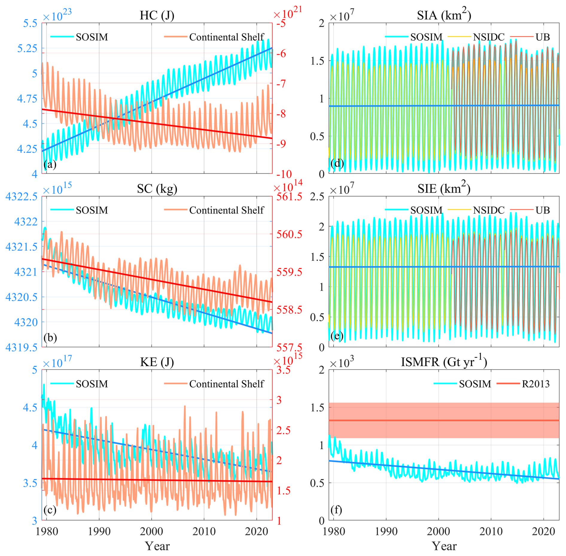
Although the drifts of the domain-integrated HC and SC exist, SOSIM still can approach a quasi-equilibrated state over shelf seas (red lines in Fig. 7a–c) that are separated from the deep ocean by the ASF. Over the continental shelf, there is a slow decline in the HC from 1979 to 1996, and thereafter there is no significant drift of the HC, with a slight increasing in the last three year (Fig. 7a). The SC over the continental shelf still has a weaker decreasing trend, yet it also rebounds in 1993 and 2015 (Fig. 7b). There is no statistically significant trend of the KE over the continental shelf (Fig. 7c). Since the drifts of HC, SC, and KE are much weaker over the continental shelf than in the deep ocean, it is expected that the ASC/ASF plays an effective role in regulating the meridional heat and salt fluxes across the continental slope (Thompson et al., 2018).

There are no significant drifts in the SIA and SIE during the interannually forced integration (Fig. 7d and e). The simulated SIA in the austral winter agrees well with observations from the UB, yet SOSIM underestimates the SIA in the austral summer (Fig. 7d). The seasonality of the simulated SIE is also stronger than observations (Fig. 7e). Since the UB has not provided observational data before 2002, we also compare the simulated sea ice with observations from the NSIDC that fully cover the period of our model integration. Compared to the observed sea ice from the NSIDC, SOSIM overestimates the seasonality of both SIA and SIE (Fig. 7d and e). Although the simulated seasonal variability of the SIA and SIE is relatively stronger than observations, the simulated interannual variabilities are comparable with observations from both the UB and NSIDC. The stronger seasonality of the SIA and SIE in SOSIM may be attributed to the zero-layer thermodynamic assumption of the sea ice model that does not store heat in the sea ice, and thereby the seasonal variability of the sea ice tends to be exaggerated.

The basal melting of ice shelves drifts towards a decline before 1990 and approaches a quasi-equilibrium afterwards (Fig. 7f). It is somehow counterintuitive that the basal melting of ice shelves drifts towards weakening when the oceanic HC drifts towards warming. Indeed, the basal melting/freezing of ice shelves is closely related to the characteristics of water masses in sub-ice-shelf cavities rather than the total HC of the ocean. Since the water intrusion into sub-ice-shelf cavities is associated with complex processes (Dinniman et al., 2016), the increase in the total HC may not enhance the basal melting of ice shelves directly.

Overall, the model equilibration varies substantially across different regions of the model domain (Figs. 6 and 7). The continental shelf and slope regions reach a quasi-equilibrium state much more rapidly than the deep ocean, with no statistically significant trends over the last two decades of the simulation. In contrast, there are persistent, albeit slow, drifts in the deep ocean throughout the integration period. Therefore, large-scale integral diagnostics should be interpreted with caution, particularly for the abyssal circulation or long-term climate variability.

3.3 Potential temperature and salinity in open oceans

The hydrographic properties of water at the sea surface layer are highly variable due to atmospheric forcing, while those of the bottom layer remain relatively stable. Therefore, the SST and SSS in the austral summer and winter are examined, while the climatological annual mean θ and S at the bottom layer are assessed. The vertical structures of zonally averaged θ and S in the Southern Atlantic sector, the Southern Pacific sector, and the Southern Indian sector are shown in three cross-sections, respectively. We also assessed the Mixed Layer Depth (MLD), which is defined as the depth where the potential density σ₀ is 0.03 kg m⁻³ larger than at the sea surface. In this subsection, we compare the simulated hydrographic properties to WOA18.

SST in the Southern Ocean is governed by coupled atmosphere–ice–ocean feedbacks, exhibiting a pronounced meridional gradient (Figs. 8 and S1 in the Supplement). In the austral summer, the retreat of sea ice exposes larger areas of open ocean, allowing increased absorption of solar radiation, leading to pronounced seasonal warming of the SST (Fig. 8a). During the austral winter, SST is thermodynamically constrained near the surface freezing point beneath the sea ice cover (Fig. 8d). The strong meridional SST gradient coincides with the marginal ice zone.

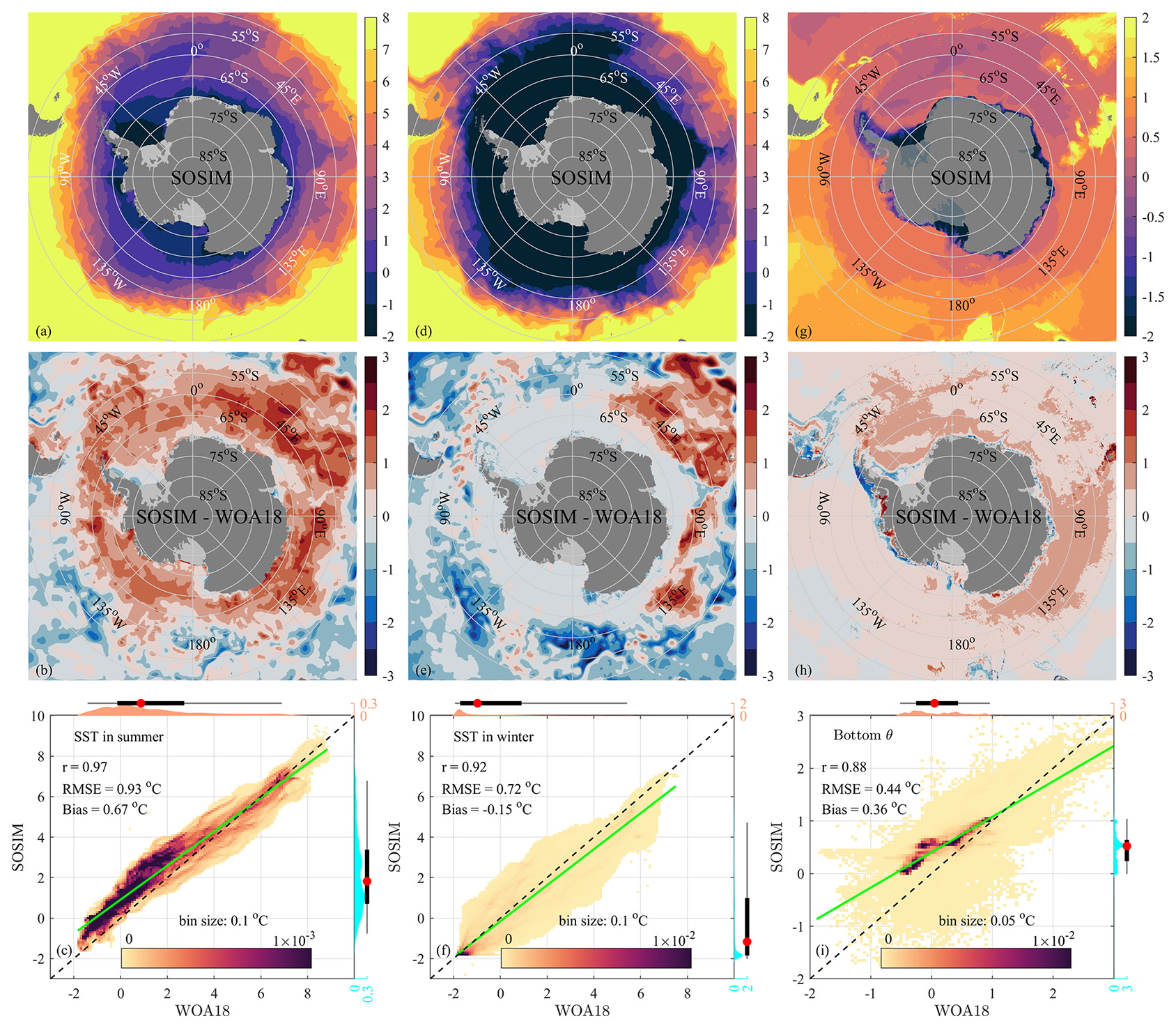
Figure 8 The horizontal distribution of θ (°C). (a) Climatological SST in summer from SOSIM. (b) The differences of SST between SOSIM and WOA18 (SOSIM minus WOA18). (c) The scatter density plot of summer SST for the deep ocean region within the inner domain (corresponding to Fig. 8a and b), with color shading indicating the proportion of data points in each bin (the bin size is reported in the panel). The black dashed line represents the 1:1 agreement line, and the green line denotes the linear regression fit. Marginal distributions show the PDF on the marginal top (WOA18, red fill) and right (SOSIM, cyan fill) axes, annotated with medians (red dots), interquartile ranges (thick black lines), and 95 % data intervals (thin grey lines) based on the kernel density estimate. r, RMSE, and mean bias are reported in the panel; p-value is only displayed when p>0.01. (d–f) As in (a–c), but for winter SST. (g–i) As in (a–c), but for the climatological annual mean θ at the bottom layer.

Summer SST biases are predominantly warm south of 50° S, while cold biases occur near open boundaries at lower latitudes (Fig. 8b). During winter, SST biases are minimal at high latitudes, with localized warm biases emerging in the mid-low latitude southern Indian Ocean sector (Fig. 8e). Since sea ice thermodynamically constrains SST near the freezing point beneath its cover, the spatial pattern of SST biases is closely related to the simulated biases of SIE. Specifically, summer warm biases align with a systematic underestimation of SIE in the model (Fig. 7e), which enhances shortwave absorption in overestimated open-water areas. The biases of the simulated sea ice are discussed in Sect. 3.7 in detail. Compared to the highly variable surface layer, the bottom layer provided more insights into the model drift (Fig. 8g and h). Weak but extensive warm biases in abyssal waters indicate the warming of simulated AABW (Fig. 8h). This basin-wide deep warming probably reflects inadequate AABW formation on continental slopes, which is further discussed in Sect. 3.6.

For statistical comparisons, the simulated summer SST in SOSIM achieves very good agreement with that in WOA18 (Fig. 8c; r=0.97, RMSE=0.93 °C) and still maintains a strong Spearman correlation in winter (Fig. 8f; r=0.92, RMSE=0.72 °C). The linear regression lines in both seasons are closely aligned with the 1:1 agreement line. SOSIM accurately captures the cold SST at the sea surface freezing point in winter, with the PDFs of both observations and simulations peaking at $\sim -\mathrm{1.8}$ °C (Fig. 8f). In summer, the PDFs of both SOSIM and WOA18 ranges from $\sim -\mathrm{1.8}$ to ∼8 °C (Fig. 8c), yet a warm mean bias is still evident in summer (0.67 °C), with PDFs of SOSIM and WOA18 peaking at ∼1.1 and ∼0.16 °C, respectively. For the bottom θ (Fig. 8i), although the regression slope deviates from unity, with a statistical overestimation of θ below 1.3 °C and a statistical underestimation above 1.3 °C, the Spearman correlation remains strong (r=0.88), with a low RMSE of 0.44 °C. The PDFs show some differences in distribution shapes (Fig. 8i), as SOSIM produces a pronounced peak at ∼0.54 °C, whereas a relatively flat distribution is present between $\sim -\mathrm{0.71}$ and ∼1 °C in WOA18.

In the Southern Ocean, θ is characterized by a thermal inversion in the vertical structure, with a cold upper layer overlying a relatively warm CDW core (upper panels in Figs. 9 and S2 in the Supplement). The cold upper layer results from intense atmospheric cooling and sea ice formation in winter, while the meridional overturning circulation brings CDW poleward at depth. Beneath this warm CDW layer, AABW forms a near-homogeneous cold reservoir that spreads equatorward, ultimately establishing a sandwich structure: a cold upper layer, a warm mid-depth layer, and a cold abyssal layer. Due to the wind-driven upwelling, isotherms slope upward and southward, shoaling most over the Antarctic Divergence Zone (∼65° S).

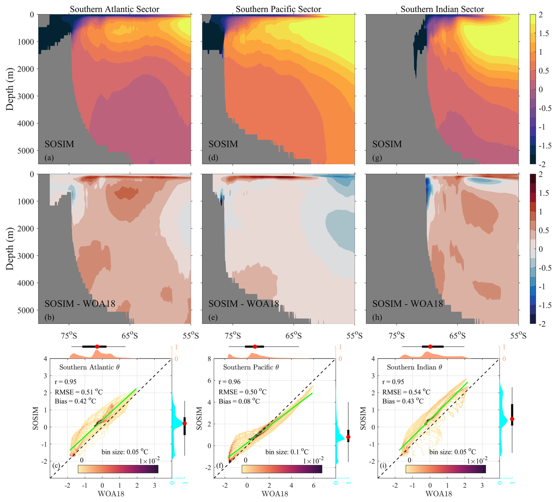
Figure 9 The vertical distribution of zonally averaged θ (°C). (a) Climatological annual mean of zonally averaged θ in the Southern Atlantic sector from SOSIM. The zonal average is calculated by omitting dry grids. (b) The differences of θ between SOSIM and WOA18 (SOSIM minus WOA18). (c) Statistical comparison of θ between SOSIM and WOA18. (d–f) As in (a–c), but for the Southern Pacific sector. (g–i) As in (a–c), but for the Southern Indian sector.

The vertical structure of zonally averaged θ reveals distinct model biases across depth layers (middle panels in Fig. 9). In the Southern Atlantic sector, broad warm biases are present, with the largest anomalies concentrated at thermocline depths (Fig. 9b). The strong subsurface biases are primarily driven by an anomalously shallow thermocline in SOSIM, which enhances upper-ocean heat retention. Consistent with these local features, horizontally basin-averaged warm biases permeate the entire water column (Fig. S3a in the Supplement). In the Southern Pacific sector, cold biases extend from low-latitude regions poleward to ∼65° S, while relatively weak warm biases emerge south of 65° S at depth (Fig. 9e). Similar to the Southern Atlantic sector, peak warm biases occur at the thermocline depth, correlated with the shallower thermocline in SOSIM. Basin-scale diagnostics reveal weak cold biases at mid-depths (from thermocline to ∼3000 m) despite abyssal warming (>3000 m; Fig. S3b). In the Southern Indian sector, strong warm biases dominate the upper mixed layer at lower latitudes, while weak cold anomalies are present below the thermocline (Fig. 9h). The subsurface cooling biases are primarily driven by a deep thermocline bias in SOSIM, which may be associated with the SIE in winter (discussed in Sect. 3.7). Horizontally basin-averaged warm biases dominate the Southern Indian sector (Fig. S3c), and the consistency at the thermocline depth likely reflects the cancellation between coastal cold anomalies and offshore warm biases. Significant seasonal variability of θ in the upper ocean (<500 m) contrasts sharply with dampened signals in the abyss (>1500 m) (Fig. S3). The pervasive warming biases at mid-depths in SOSIM likely originate from overestimated eddy activity (discussed in Sect. 3.4), which may enhance eddy-mediated poleward heat transport.

Across all three Southern Ocean sectors, SOSIM exhibits exceptional performance in reproducing the statistical characteristics of the zonally averaged θ (lower panels in Fig. 9). The Spearman correlation coefficients range from 0.95 to 0.96, with RMSE values ranging from 0.50 to 0.54 °C. Warm mean biases are present in the Southern Atlantic (Fig. 9c; 0.42 °C) and Southern Indian (Fig. 9i; 0.43 °C) sectors, while a very slight warm mean bias (0.08 °C) is present in the Southern Pacific sector (Fig. 9f). In the Southern Atlantic and Southern Indian sectors, the distributions of PDFs of SOSIM are shifted toward warmer θ compared to WOA18, with simulated peaks occurring above 0 °C versus observed peaks below 0 °C.

SSS in the Southern Ocean is governed by ice–ocean freshwater fluxes and wind-driven mixing, exhibiting strong meridional gradients and pronounced zonal asymmetry (Figs. 10 and S4 in the Supplement). Distinct from the spatial pattern of SST, the freshest SSS is present to the north of West Antarctica, implying the influence of ice-shelf meltwater discharges from West Antarctic glaciers. During austral winter, brine rejection from sea ice formation elevates SSS beneath sea ice cover, with the maximum salinification in coastal polynyas, while Ekman divergence confines high-salinity surface waters to the south flank of the Antarctic Divergence Zone. In the austral summer, widespread sea ice melt depresses SSS around Antarctica, with the most intense freshening centered in the Bellingshausen Sea. The meltwater of sea ice forms a shallow freshwater cap that persists until autumn, suppressing vertical mixing and enhancing upper-ocean stratification.

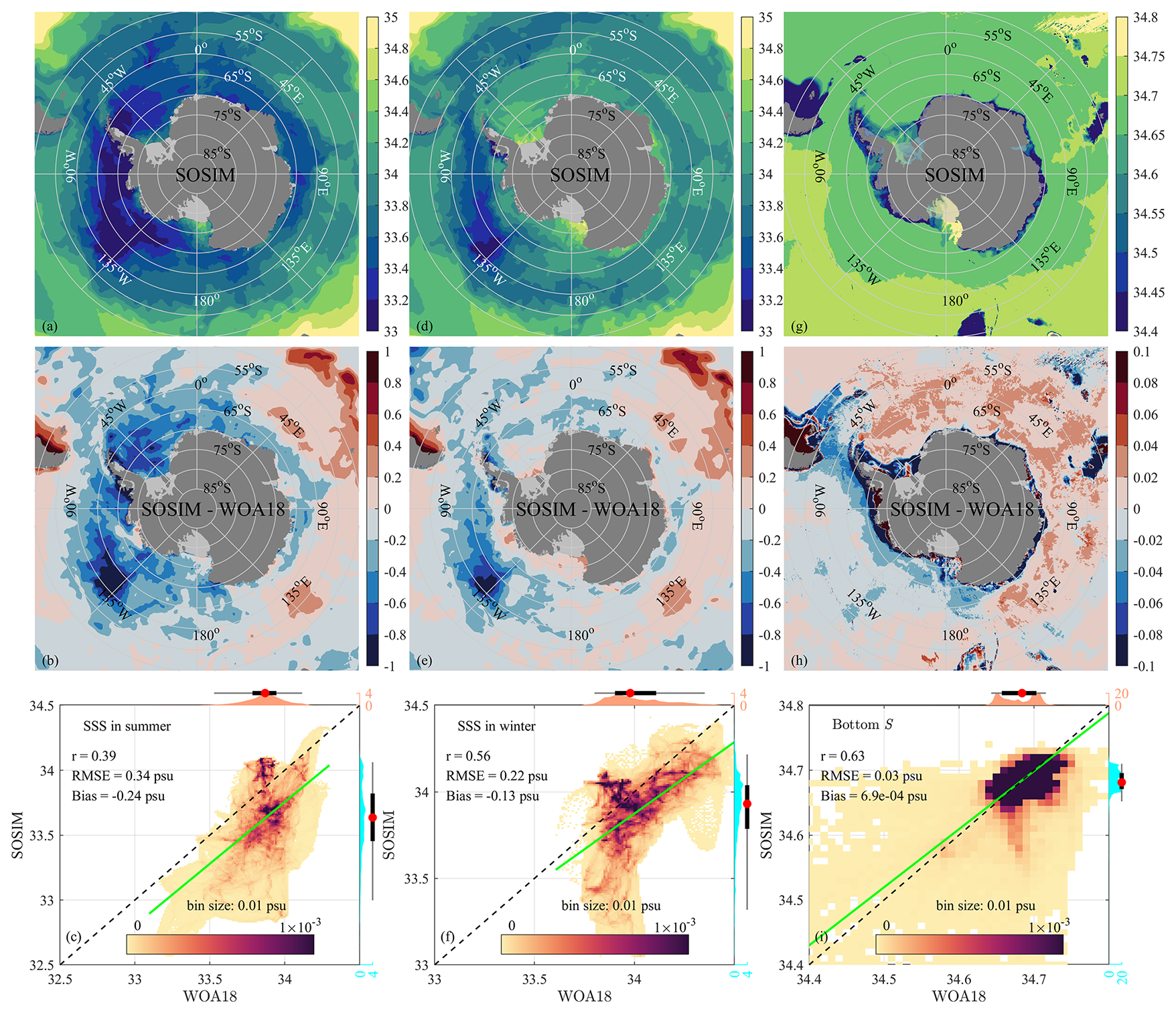
Figure 10 As in Fig. 8, but for the horizontal distribution of S (psu).

Summer SSS biases are predominantly fresh in the Weddell and Ross Seas, while saline biases occur in the Southern Indian sector (Fig. 10b). During winter, strong fresh biases are present in the Southern Pacific sector, with a localized fresh core emerging in the eastern Ross Sea (Fig. 10e). Unlike SST, SSS under sea ice is more sensitive to the phase changes (freezing/melting) of sea ice than to the SIE, resulting in larger SSS biases relative to SST at high latitudes in winter. Contrasting with saline biases in the Southern Atlantic and Indian sectors, the drift of S at the bottom layer remains relatively weak in the Southern Pacific sector (Fig. 10h), characterized by fresh biases. Although positive salinity anomalies favor increased AABW density, the density of seawater still depends on the combined thermohaline changes of both θ and S. Indeed, SOSIM ultimately produces lighter AABW in the Southern Ocean (further analyzed in Fig. 14). While continental shelf salinity comparisons between SOSIM and WOA18 are shown in this section, the assessment of shelf waters is deferred to Sect. 3.5.

SOSIM shows relatively greater challenges in reproducing the statistical characteristics of S. The simulated SSS in summer and winter exhibit weak (r=0.39) to moderate (r=0.56) Spearman correlations with WOA18, respectively (Fig. 10c and f). Negative mean biases of −0.24 and −0.13 psu are present, and the regression lines are offset below the 1:1 line (Fig. 10c and f). SOSIM does not reproduce the distinct peak observed in the WOA18 PDF in summer (at ∼33.87 psu), instead generating relatively flat distributions between ∼32.82 and ∼34.13 psu. The bottom S shows a moderate Spearman correlation of 0.63 between SOSIM and WOA18, with a low RMSE of 0.03 psu and a negligible mean bias (Fig. 10i). Meanwhile, the regression exhibits good agreement with unity (Fig. 10i). Yet, SOSIM does not capture the bimodal structure of bottom S present in the WOA18 PDF, although SOSIM produces a similar range distribution, with high probability densities concentrated between ∼34.63 and ∼34.73 psu.

S in the Southern Ocean exhibits distinct vertical stratification shaped primarily by the ice–ocean freshwater exchange, wind-driven advection, and meridional overturning circulation (upper panels in Figs. 11 and S5 in the Supplement). Similar to θ in the Southern Ocean, S is also characterized by a three-layer stratification, with a fresh upper layer overlying a pronounced saline CDW core and a relatively saline deep layer. Driven by the wind upwelling and meridional overturning circulation, isohalines also slope upward and poleward, with the minimum depth over the Antarctic Divergence Zone.

Figure 11 As in Fig. 9, but for the vertical distribution of zonally averaged S (psu).

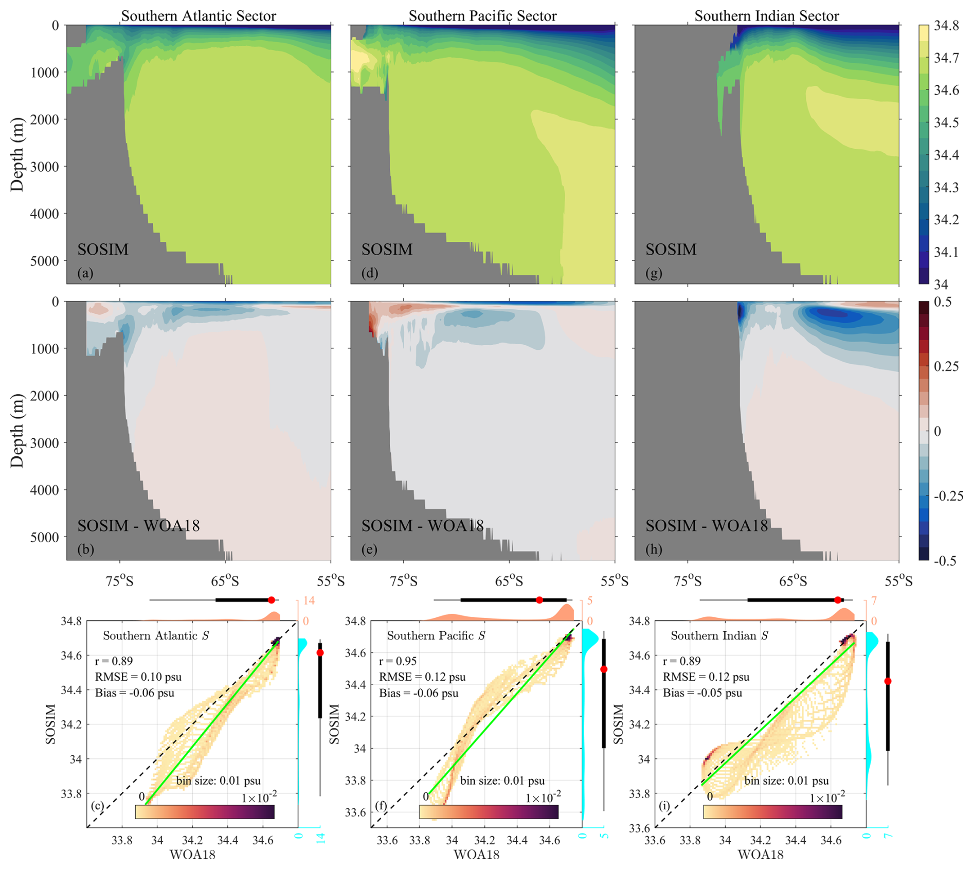
The vertical structure of zonally averaged S exhibits distinct biases across depth layers and ocean sectors (middle panels in Fig. 11). In the Southern Atlantic and Pacific sectors, widespread surface fresh biases occur (Fig. 11b and e), consistent with assessments shown in Fig. 10. Subsurface fresh bias cores are evident at halocline depths, attributable to the anomalously deep halocline simulated in SOSIM (Fig. 11a and d). In contrast to the South Atlantic and South Pacific sectors, surface fresh biases in the Southern Indian sector do not extend south of 55° S, and saline biases occur north of 60° S (Fig. 11h). The Southern Indian sector hosts the strongest subsurface fresh bias core among all basins near 60° S (Fig. 11h), associated with an excessive halocline depth bias in SOSIM (Fig. 11g and h). Within the abyssal layers, weak fresh biases are prevalent in the South Pacific sector (Fig. 11e), whereas weak saline biases are characterized in the South Atlantic and South Indian sectors (Fig. 11b and h). Horizontally averaged basin-scale diagnostics reveal a good agreement between SOSIM and WOA18 within the Southern Atlantic sector (Fig. S6a in the Supplement). For the Southern Pacific Ocean sector, fresh biases dominate the surface layer, and saline biases dominate at ∼1000 m depth (Fig. S6b). Pronounced biases occur in the mid-depth layer of the Southern Indian sector, peaking as the strongest fresh bias occurring at ∼600 m depth (Fig. S6c). Compared to θ, biases of S are comparatively modest in the abyssal layer, and SOSIM generally reproduces the observed S at depths >2000 m (Fig. S6).

SOSIM also performs well in simulating the statistical characteristics of zonally averaged S (lower panels in Fig. 11), particularly in the Southern Pacific sector (r=0.95) (Fig. 11f). Slight negative mean biases, ranging from −0.05 to −0.06 psu, are present in all three sectors. The primary salinity distributions (from ∼33.75 to ∼34.75 psu) are well captured in the PDFs across three sectors, with both SOSIM and WOA18 sharing the main peak at ∼34.68 psu. Yet, SOSIM struggles to reproduce secondary salinity features. Specifically, SOSIM misses the weak peak at ∼33.99 psu in the Southern Pacific sector and shifts the secondary peak from ∼33.9 to ∼34.01 psu in the Southern Indian sector (Fig. 11i).

The mixed layer in the Southern Ocean serves as a critical layer for ocean–sea ice–air interactions, water mass transformation, and carbon sequestration. There are strong spatiotemporal variabilities in the MLD (Figs. 12 and S7 in the Supplement). The deep MLD is located between 50 and 65° S along the ACC belt, while the shallower MLD prevails over Antarctic marginal seas and subtropical regions. Driven by the joint modulation of buoyancy fluxes (e.g., salt fluxes associated with sea ice freezing/melting and heat flux dominated by solar radiation), wind forcing, and oceanic turbulent mixing, the MLD exhibits a pronounced seasonal cycle. In summer, the MLD is typically shallow across the Southern Ocean (Fig. 12a), though locally reaches ∼100 m between 50 and 65° S. Over shelf seas around Antarctica, freshwater from coastal ice melt enhances stratification, constraining the MLD to shallower depths (<20 m) than in the subantarctic region. In winter, deep convection generates the deepest mixed layers in the Southern Ocean, where basin-scale MLD exceeds 300 m and peaks at ∼500 m in the Southern Pacific Ocean sector (Fig. 12d). Such deep winter mixed layers ventilate SAMW and AAIW, directly regulating the global overturning circulation.

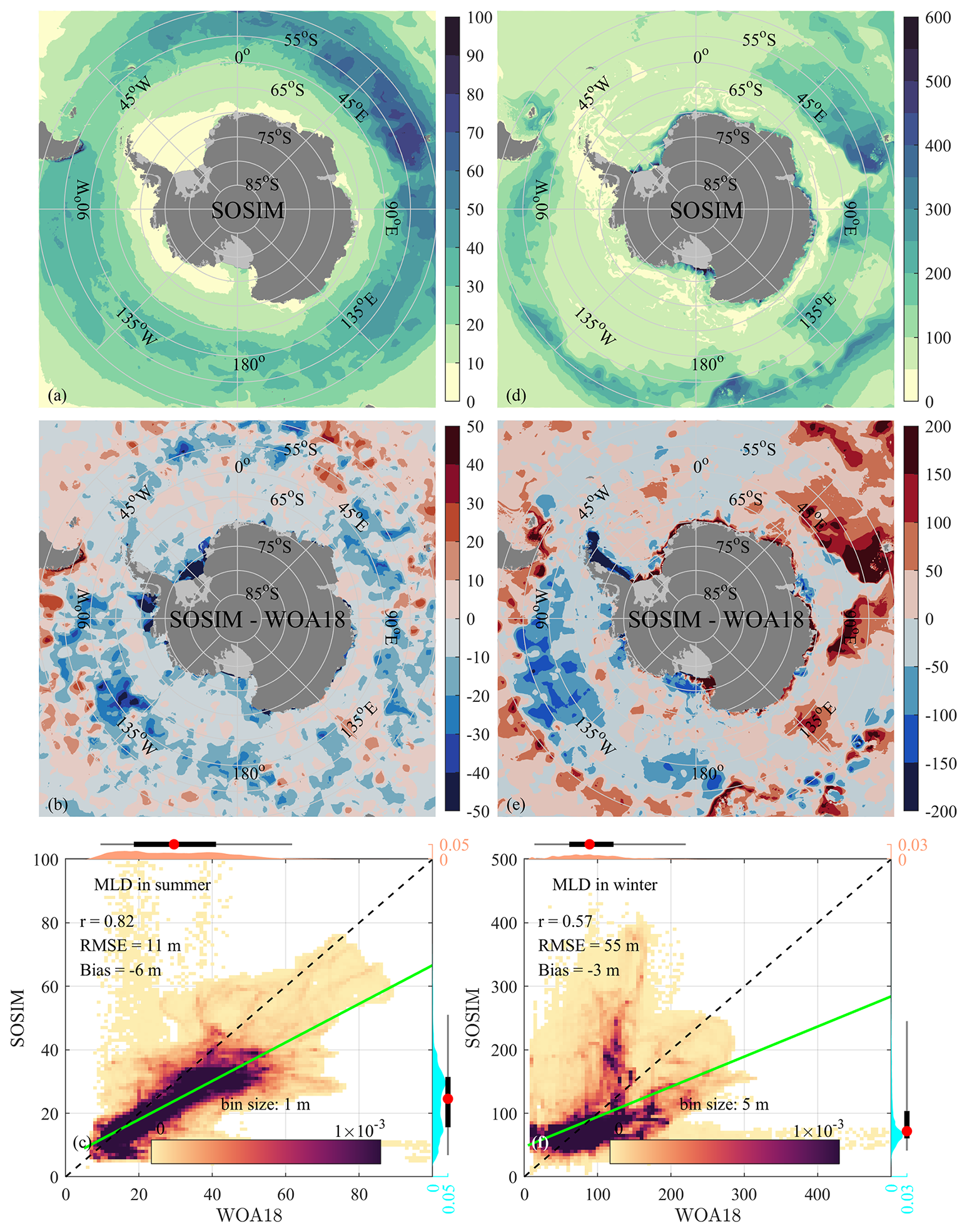
Figure 12 The horizontal distribution of MLD (m). (a) The MLD of SOSIM in the austral summer. (b) The differences of MLD between SOSIM and WOA18 (SOSIM minus WOA18). (c) Statistical comparison of MLD between SOSIM and WOA18. (d–f) As in (a–c), but for the MLD in the austral winter.

In summer, SOSIM underestimates the MLD across the ACC belt, with the largest shallow biases (>50 m) occurring in the South Pacific sector (Fig. 12b). In winter, persistent shallow biases prevail in the South Pacific sector, whereas substantial deep biases (>200 m) emerge in the Southern Indian sector (Fig. 12e). The shallow MLD biases are likely due to excessive freshwater input and consequent fresh SSS biases, especially in the Southern Pacific sector (Fig. 10b and e). These deep MLD biases in the winter Southern Indian collocate spatially with saline SSS biases (Fig. 10b and e), coinciding with lower SIC biases (discussed in Sect. 3.7). WOA18 exhibits relatively large uncertainties in the MLD over Antarctic coastal regions (Fig. S7), and thereby we have not further discussed the MLD biases over shelf seas in this subsection.

Compared to WOA18, SOSIM shows varying performance in simulating the statistical characteristics of the MLD between seasons, with higher skill in summer than in winter (lower panels in Fig. 12). In summer, SOSIM shows good agreement with observations from WOA18 (Fig. 12c), evidenced by a strong Spearman correlation (r=0.82) and a relatively low RMSE of 11 m. Yet, the linear regression line deviates from the 1:1 line, with an overestimation of MLD for values shallower than 15 m and an underestimation for values deeper than 15 m. The PDFs reveal that the simulated summer MLD distribution (from ∼5 to ∼50 m) is narrower than the observed range (from ∼5 to ∼60 m). In contrast, the performance of SOSIM in simulating the winter MLD is relatively weaker (Fig. 12f), showing a moderate correlation (r=0.57) and a larger RMSE of 55 m. The regression line exhibits a stronger deviation, statistically overestimating the shallow MLD (<92 m) and underestimating the deep MLD (>92 m). The distributional characteristics also differ notably. While the observed winter MLD from WOA18 shows a broad and flat distribution from ∼5 to ∼200 m, SOSIM produces a pronounced peak at ∼68 m, with an overall distribution concentrated between ∼35 and ∼150 m. These comparisons suggest that the simulated winter MLD in SOSIM does not have good agreement with the statistical distribution in WOA18.

Within the domain of SOSIM, the major oceanic fronts consist of the SAF, PF, and Southern Antarctic Circumpolar Current Front (SACCF), associated with boundaries of water masses and dynamical regimes (Figs. 13 and S8 in the Supplement). The band between the SAF and PF is the Polar Frontal Zone, where AAIW is formed and subducts into deep layers; the band between the PF and SACCF is the Antarctic Zone, where CDW shoals southward across the ACC (Whitworth et al., 1998). We adopt the definition of these oceanic fronts from Orsi et al. (1995). The SAF is defined as the 4 °C isotherm at 400 m depth, the PF is defined as the 2.2 °C isotherm at 800 m depth, and the SACCF is defined as the 1.8 °C isotherm at 800 m depth.

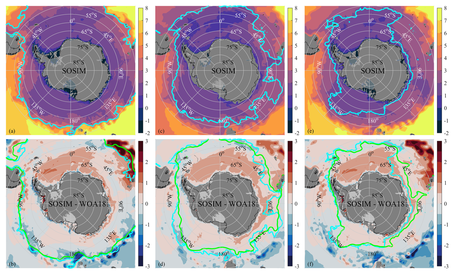
Figure 13 The circumpolar distribution of the SAF, PF, and SACCF, with θ (°C) at corresponding depths in color. (a) The SAF (the cyan line, 4 °C isotherm) and θ (°C) at 400 m depth in SOSIM. (b) The differences of θ (°C) at 400 m between SOSIM and WOA18 (SOSIM minus WOA18), with the green line indicating the SAF from WOA18. (c, d) As in (a, b), but for the PF (2.2 °C isotherm) and θ (°C) at 800 m depth. (e, f) As in (a, b), but for the SACCF (1.8 °C isotherm) and θ (°C) at 500 m depth.

Since we adopt the definitions of circumpolar fronts based on θ, the meridional displacements of circumpolar fronts in SOSIM relative to those in WOA18 are associated with θ biases. Accordingly, poleward biases of fronts are related to warm biases, and vice versa. The SAF is generally aligned along 55° S in the South Pacific sector (Fig. 13a), and SOSIM reproduces the position of the SAF (Fig. 13b). Within the Southern Atlantic and Southern Indian sectors, portions of the SAF reside outside the SOSIM domain. Where the front traverses the model interior in the Southern Indian sector, a southward displacement occurs, associated with a pronounced warm bias core near the corner of the SOSIM domain. The PF is largely contained within the SOSIM domain (Fig. 13c). In the Southern Atlantic sector, the PF in SOSIM shows good agreement with WOA18 (Fig. 13d). Evident southward biases in the PF are identified in the Southern Indian sector, particularly across the Valdivia Abyssal Plain and Davis Sea. Conversely, the simulated PF exhibits a slight northward bias in the Southern Pacific sector. The SACCF predominantly resides south of 55° S within the SOSIM domain (Fig. 13e), sufficiently far from open boundaries. There is significant spatial variability in the proximity of the SACCF to the Antarctic continental shelf, with the closest approach occurring west of the Antarctic Peninsula and maximal separation emerging in the Weddell and Ross Sea sectors, where segments extend north of 55° S. The SACCF in SOSIM agrees well with that in WOA18 across most sectors, except for some southward biases in the Southern Indian sector (Fig. 13f).

Thermodynamic θ–S diagrams serve as a useful diagnostic for evaluating water mass representation in ocean models, providing insights into simulated thermohaline structure and stability (Figs. 14 and S9 in the Supplement). By mapping volumetric distributions in θ–S space, the θ–S analysis shows the volume (V) of water masses in the SOSIM domain and quantifies drifts in water mass cores in a long-term integration. Characterized by θ colder than the sea surface freezing point, ISW is expected to be reproduced by SOSIM. The freezing point of sea water T_f is calculated as:

$$\begin{array}{}\text{(13)}& T_{\mathrm{f}}=aS+b+cP\end{array}$$

where a is $-\mathrm{5.73}\times {\mathrm{10}}^{-\mathrm{2}}$ °C psu⁻¹, b is $\mathrm{8.32}\times {\mathrm{10}}^{-\mathrm{2}}$ °C, c is $-\mathrm{7.61}\times {\mathrm{10}}^{-\mathrm{2}}$ °C dbar⁻¹, and P is the pressure. For the surface layer, P is fixed at 0, and the surface freezing point is dominated by S (red lines in Fig. 14).

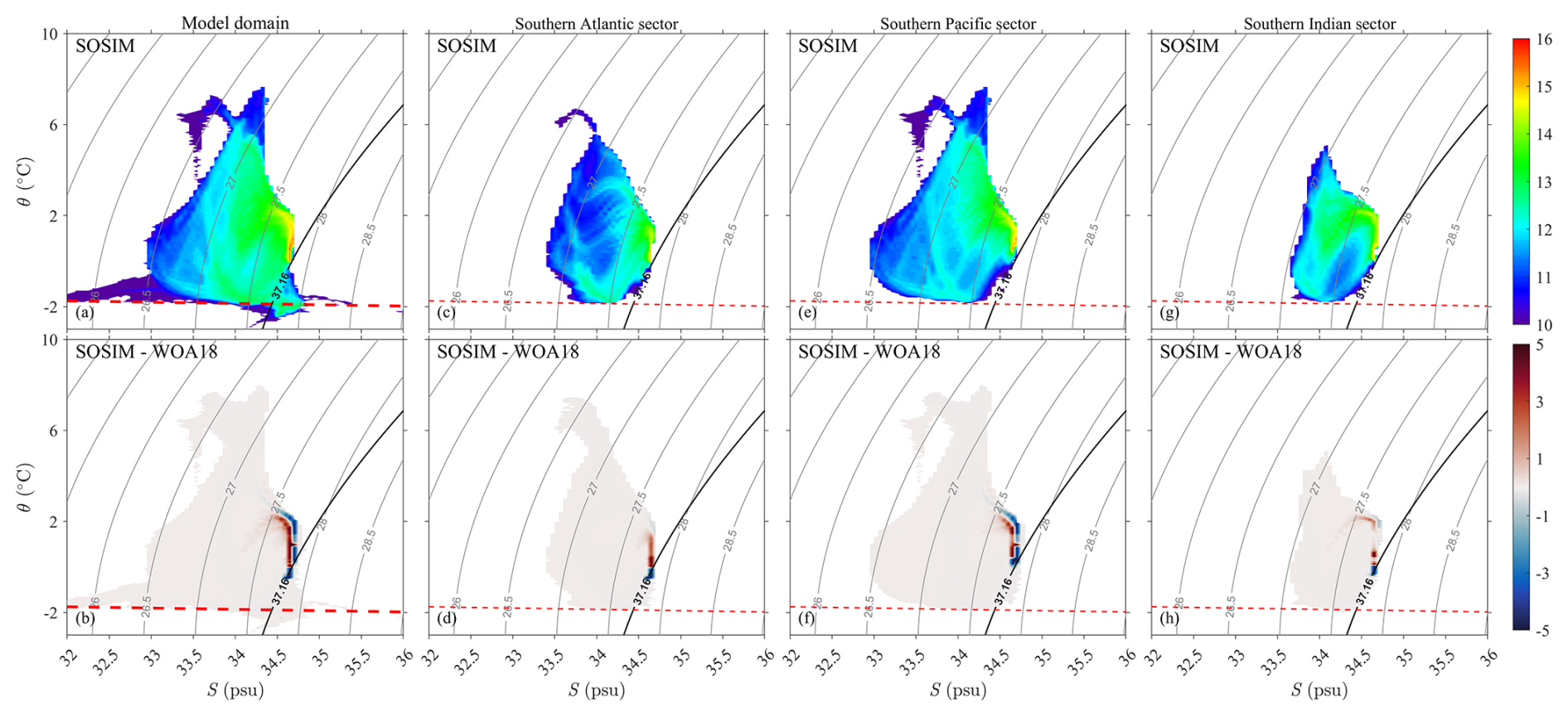
Figure 14 (a) Climatological water mass volume (log 10 (V), m³) distribution in θ–S space (bins of 0.05 °C by 0.05 psu size) in the inner model domain in SOSIM, superimposed with potential density σ₀ (grey lines) in contour intervals of 0.5 kg m⁻³. The red dashed line denotes the surface freezing point of seawater. The black lines denote the σ₂ contours of 37.16 kg m⁻³, indicating the threshold between CDW and AABW (Orsi et al., 1999). (b) The differences in water mass volume between SOSIM and WOA18 (SOSIM minus WOA18). (c, d), (e, f), and (g, h) As in (a, b), but for the Southern Atlantic sector, the Southern Pacific sector, and the Southern Indian sector, respectively.

Within the SOSIM inner domain, water masses in WOA18 occupy the θ–S space ranging from −2 to 8 °C and 33 to 34.8 psu, and CDW has the largest volume between −1 and 2 °C and ∼34.7 psu (Fig. S9). The absence of ISW in WOA18 is because it does not incorporate hydrographic observations from beneath ice shelves. SOSIM generally reproduces water mass distributions in the θ–S space as WOA18 (Fig. 14a). Additionally, SOSIM reproduces ISW, with evident volume present below the sea surface freezing point. The low S water extending to 32 psu in the cold θ class of $\sim -\mathrm{2}$ °C should be associated with shelf waters that are not present in the deep oceans (Fig. 14a). Yet, the volume-maximized CDW core in SOSIM is warmer and fresher than in WOA18 (Fig. 14b), shifted to 0–2 °C and ∼34.6 psu. Beyond the shelf seas, the volumetric θ–S distributions in SOSIM are in good agreement with WOA18 (Fig. 14c–h); however, systematic biases are also evident in the core properties of CDW. In the Southern Atlantic and Southern Indian sectors, the CDW core is biased warm (Fig. 14d and h), while it shifts to a warmer and fresher state in the Southern Pacific sector (Fig. 14f). Notably, AABW has virtually vanished in SOSIM (Fig. 14c, e, and g). Considering dense SW has been reproduced by SOSIM (Fig. 14a), the reduction of AABW is likely induced by the absence of its formation over the Antarctic continental slope, where AABW is produced by mixing between dense SW and surrounding water masses (discussed in Sect. 3.6).

3.4 Circulations and eddies in the open oceans

To evaluate the simulated circulations, the large-scale volume transport is assessed against the observational estimate of C2016 and the reanalysis product SOSE, and the simulated surface MKE and EKE are compared with satellite altimetry data distributed by AVISO. The large-scale circulations in the Southern Ocean are dominated by the ACC, characterized as a strong frontal jet streaming eastward around Antarctica. The path of the ACC is largely constrained by the topography, generating large-scale meanders and narrow filaments. To the south of the ACC, cyclonic circulations of subpolar gyres dominate the subpolar seas, including the Weddell and Ross gyres. The sea surface kinetic energy field is characterized by high MKE along the ACC jet and elevated EKE downstream of major topographic features.

Despite its limited coverage in subpolar regions (Fig. S10a in the Supplement), the C2016 dataset still delineates the structure and transport of the ACC. The barotropic streamfunction Ψ from C2016 reveals tightly packed isolines between 50 and 65° S, corresponding to a volume transport through the Drake Passage to ∼175 Sv. To further elucidate the structure of subpolar gyres, we calculated Ψ from SOSE by integrating the zonal velocity field (Fig. S10b). In contrast to the negative values of Ψ from C2016, positive values across the ACC in SOSE are induced by the northward integration starting from the Antarctic continental boundary. The SOSE yields an ACC transport of ∼164 Sv through the Drake Passage, consistent with the estimation from C2016 and the observational benchmark of 173 Sv from Donohue et al. (2016). Negative values of Ψ in SOSE represent cyclonic circulations, clearly capturing the Weddell and Ross gyres (Fig. S10b). The Weddell Gyre has a broad spatial extent, stretching eastward from the Antarctic Peninsula to approximately 45° E, with a maximum transport of ∼40 Sv. The Ross Gyre is located between 135° W and 180°, with a peak transport of ∼30 Sv.

Compared to C2016 and SOSE products, Ψ simulated by SOSIM shows a significantly weaker ACC, with the transport of only ∼77 Sv across the Drake Passage (Fig. 15a). Such an underestimation of the ACC in SOSIM may be largely attributed to the open boundaries being positioned too close to the ACC path, where uncertainties in the open boundary conditions may restrict the full development of the current within the model domain. Furthermore, SOSIM simulates an overly energetic eddy field (discussed in Fig. 16). The excessive eddy activities suggest an intensified energy cascade, wherein MKE from the ACC may be disproportionately transferred into EKE. Indeed, the underestimation of ACC transport appears to be a systematic bias in high-resolution model configurations (Farneti et al., 2015; Kiss et al., 2020). Meanwhile, subpolar gyres in SOSIM are stronger than in SOSE (Fig. 15b), most notably for the Weddell Gyre. Yet, these biases in subpolar gyres do not appear to significantly affect the simulated currents over the Antarctic continental slope and shelf regions.

Figure 15 The barotropic stream function. (a) The climatological Ψ (Sv) estimated from SOSIM. Negative cells denote cyclonic circulations. (b) The differences of Ψ between SOSIM and SOSE (SOSIM minus SOSE).

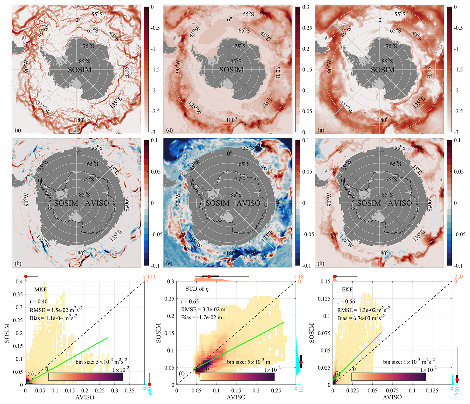
Figure 16 The sea surface Kinetic Energy and the variability of η. (a) The log ₁₀(MKE_surf) (m² s⁻²) in SOSIM. (b) The differences of sea surface MKE between SOSIM and AVISO (SOSIM minus AVISO). The grey region over the open ocean indicates the absence of year-round data in the AVISO. (c) Statistical comparison of log ₁₀(MKE_surf) between SOSIM and AVISO. (d–f) As in (a–c), but for the STD of η (m). (g–i) As in (a–c), but for the log ₁₀(EKE_surf) (m² s⁻²).

The surface climatological velocity in SOSIM is evaluated by comparing with observations from the AVISO (Figs. 16 and S11 in the Supplement), including the spatial pattern of MKE_surf and EKE_surf. The standard deviation (STD) of η is also calculated to show the statistical characteristics of η^′ that is related to the EKE. Due to persistent sea ice cover, the AVISO satellite altimetry product lacks data in subpolar regions (Fig. S11). Within the ACC region, the MKE_surf features multiple high-speed jets organized into distinct zonal bands (Fig. S11a). These jets are typically aligned with major bathymetric features such as mid-ocean ridges, plateaus, and fracture zones, which steer and stabilize the flow. In contrast, the STD of η and EKE_surf display more diffuse and widespread distributions (Fig. S11b and c). Nonetheless, their most intense values are generally found downstream of large topographic obstacles, including submarine plateaus and ridges.

There is a striking resemblance in the MKE_surf between SOSIM and the AVISO, with narrow filamentary structures present across the ACC region (Fig. 16a and b). SOSIM also captures the spatial pattern of η^′ and EKE_surf well (Fig. 16d and g). Yet, the STD of η in the AVISO is larger than in SOSIM (Fig. 16e), while the simulated EKE_surf is stronger than observations (Fig. 16h). Typically, stronger η variability is associated with higher EKE_surf. Such a discrepancy between η^′ and EKE_surf relative to observations may stem from differences in the spatial resolution of SOSIM and AVISO and the methodology for deriving surface geographic currents. Specifically, the spatial resolution of the AVISO is 0.25°×0.25°, while SOSIM has a horizontal resolution of ∼5 km, enabling SOSIM to resolve smaller eddies that cannot be captured by the AVISO. Moreover, the diagnosed EKE_surf depends directly on the spatial gradient of η^′ rather than its temporal variability, implying that the spatially noisier η^′ in high-resolution SOSIM can lead to elevated EKE_surf values. In addition, the optimal interpolation adopted in generating the AVISO product from along-track satellite data tends to smooth spatial gradients of η^′, resulting in an underestimation of the EKE_surf (Chelton et al., 2011; Chambers, 2018). Overall, the simulated spatial patterns of the MKE_surf, STD of η, and EKE_surf in SOSIM are in broad-scale agreement with observations from the AVISO, with elevated MKE_surf, η^′, and EKE_surf hosted in the ACC. Furthermore, SOSIM reveals strong MKE_surf, EKE_surf and η^′ over the Antarctic continental slope where there is limited data in the AVISO.

The simulated surface MKE shows a weak positive correlation with observations from AVISO (r=0.40) and an RMSE of $\mathrm{1.5}\times {\mathrm{10}}^{-\mathrm{2}}$ m² s⁻² (Fig. 16c). There is a significant downward offset of the linear regression line from the 1:1 line. This deviation may be attributable to the mismatch in horizontal resolution between SOSIM (∼5 km) and the original AVISO product (0.25°). The coarser resolution of AVISO leads to broader representations of spatial features, such as frontal jets, which can result in higher MKE values than SOSIM in some regions. Conversely, the higher resolution of SOSIM allows it to resolve finer-scale flow structures that are smoothed out in AVISO, contributing to higher MKE values in such regions. However, since the PDFs for both SOSIM and observations peak at $\sim \mathrm{1}\times {\mathrm{10}}^{-\mathrm{4}}$ m² s⁻² and are concentrated near this value, the overall dynamic range of SOSIM still appears constrained within the range of observations. The simulated STD of η shows a moderate correlation (r=0.65) with satellite observations (Fig. 16f), with a negative mean bias of $-\mathrm{1.7}\times {\mathrm{10}}^{-\mathrm{2}}$ m. The regression line is offset below the 1:1 line, and the PDF of SOSIM simulates a narrower and shifted distribution (from ∼0.02 to ∼0.15 m) compared to the observations (from ∼0.04 to ∼0.15 m), with the peak of the simulated distribution skewed towards lower values. The simulated EKE in SOSIM captures the observed variability with a moderate correlation (r=0.56) and an RMSE of $\mathrm{1.3}\times {\mathrm{10}}^{-\mathrm{2}}$ m² s⁻² (Fig. 16i). The regression line runs approximately parallel to but above the 1:1 line, with a positive mean bias of $\mathrm{6.7}\times {\mathrm{10}}^{-\mathrm{3}}$ m² s⁻². While the PDF of observed EKE exhibits a pronounced peak at $\sim \mathrm{8.4}\times {\mathrm{10}}^{-\mathrm{4}}$ m² s⁻², the simulated EKE from SOSIM shows a relatively flatter distribution from 0 to $\sim \mathrm{2.1}\times {\mathrm{10}}^{-\mathrm{2}}$ m² s⁻². Overall, SOSIM dilutes the EKE more broadly, while the EKE is concentrated at a specific scale in observations.

3.5 Potential temperature and salinity over the continental shelf

Shelf seas around the Antarctic continent are key regions for the production of AABW and the stability of ice shelves. Intrusion of warm CDW and MCDW represents an important heat source that greatly contributes to the basal melting of ice shelves, while the formation of dense SW serves as a crucial precursor to AABW. We assess the simulated bottom water masses by comparison with hydrographic observations from the MEOP rather than using WOA18, due to the uncertainties in WOA18 over Antarctic shelf regions. Given the spatiotemporal scarcity of observational profiles across the shelf, we constructed a gridded climatological annual mean based on MEOP data by following Dinh et al. (2024). Although this approach does not capture the seasonal variability, it provides a more reliable reference than WOA18 for the shelf region, despite incomplete spatial coverage. In addition to bottom water mass properties, we also evaluate the meridionally averaged vertical structures of θ and S.

The most pronounced CDW intrusion occurs on the continental shelf of the WAP, Bellingshausen, and Amundsen sectors, characterized by a maximum θ exceeding 1.5 °C (upper panels in Figs. 17 and S12 in the Supplement). MCDW intrusion is also present over the East Antarctica sector. The saltiest SW is found in the western Ross sector, particularly within the Drygalski Trough, indicating its role as a major source region of AABW. In contrast, the freshest SW is found in the Amundsen sector, with salinity values as low as 34.1 psu, implying the influences of freshwater input from the strong basal melting of local ice shelves. SOSIM can reproduce the large-scale spatial distribution of observed bottom θ and S over the Antarctic continental shelf, with the warmest water in the West Antarctica and saltiest SW in the Ross sector.

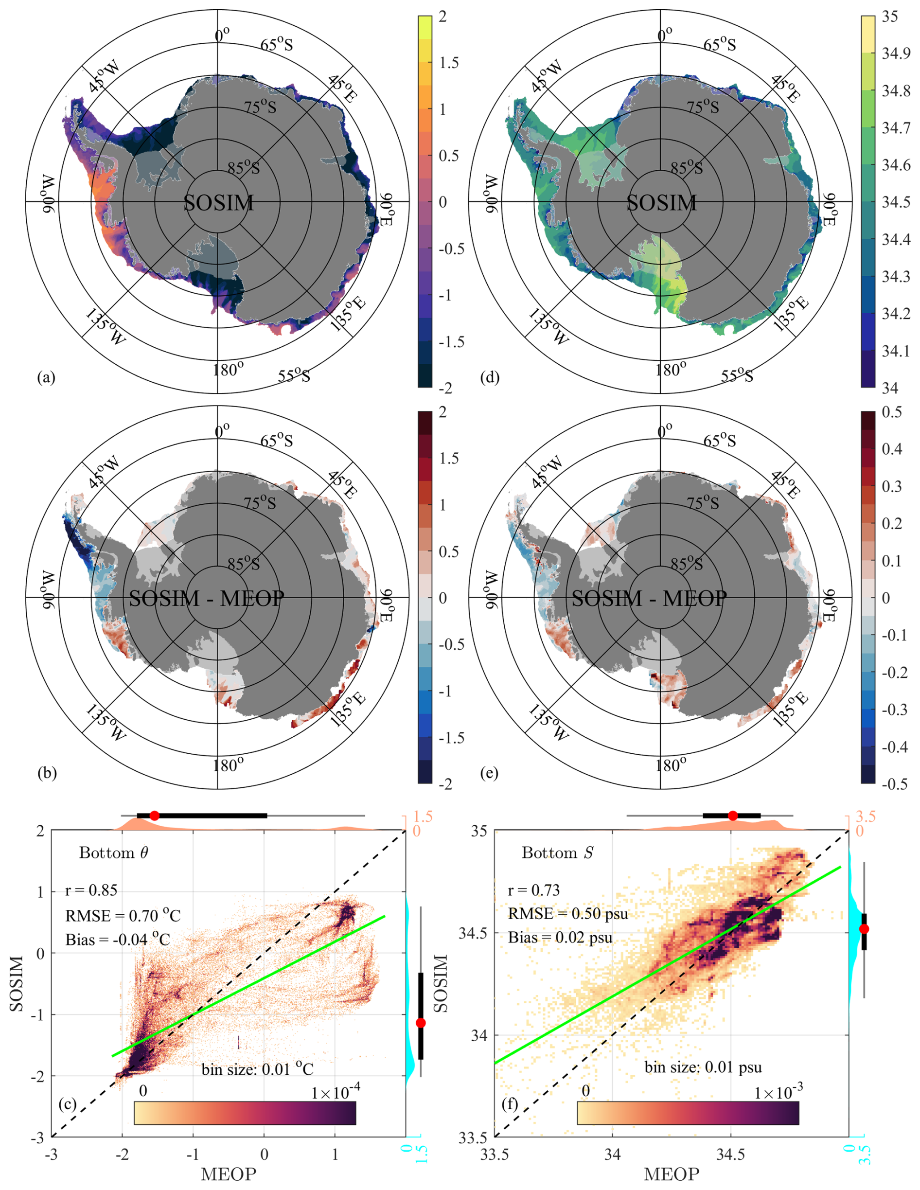
Figure 17 The horizontal distribution of θ (°C) and S (psu) over the continental shelf. (a) Climatological θ at the bottom layer in SOSIM. (b) The differences of bottom θ between SOSIM and the gridded MEOP (SOSIM minus MEOP). (c) Statistical comparison of bottom θ between SOSIM and WOA18. (d–f) As in (a–c), but for bottom S (psu).

Distinct regional biases in the simulated bottom water properties over the Antarctic shelf are revealed by the comparison between SOSIM and MEOP (Fig. 17b and e). On the shelves of the WAP and Bellingshausen sectors, SOSIM shows cold and fresh biases, with the strongest cold biases reaching $\sim -\mathrm{2}$ °C in the WAP sector, indicating an underestimation of CDW intrusion. In contrast, the Amundsen sector is characterized by a warm and salty bias, which suggests an excessive simulated intrusion of CDW. Similar warm and salty biases are present in the Ross and East Antarctica sectors, with the strongest warm biases reaching ∼1.5 °C in the East Antarctica sector. The warm bias over the outer shelf coincides with overly strong MCDW intrusion, while the salty bias on the inner shelf in the Ross sector is consistent with overestimated local sea ice production (discussed in Sect. 3.7). Relatively small temperature and salinity deviations are simulated in the Amery and Weddell sectors, implying a relatively good representation of bottom properties.

For the bottom potential θ on the continental shelf, SOSIM shows a strong correlation with observations from MEOP (r=0.85), with an RMSE of 0.7 °C and a negligible mean bias of −0.04 °C (Fig. 17c). The linear regression line has a slope lower than unity, leading to a statistical overestimation of θ for values below −1 °C and a statistical underestimation for values above −1 °C. The PDFs of both SOSIM and MEOP share a primary peak near the surface freezing point of $\sim -\mathrm{1.8}$ °C, yet SOSIM does not reproduce the secondary peak observed at ∼1.1 °C, instead showing a relatively flat distribution between $\sim -\mathrm{1}$ and ∼1 °C. Regarding the bottom S on the shelf (Fig. 17f), SOSIM shows a good correlation (r=0.73) with MEOP, with an RMSE of 0.5 psu and a mean bias of 0.02 psu. The regression line exhibits a lower slope than unity, statistically overestimating S below 34.5 psu and underestimating S above this threshold. While both the observed and simulated PDFs cover a similar range (from ∼34.10 to ∼34.80 psu), SOSIM produces a single prominent peak at ∼34.59 psu, whereas the MEOP observations are characterized by a bimodal distribution with peaks at ∼34.51 and ∼34.69 psu.

The structure of meridionally averaged θ over the Antarctic shelf (the shelf region shown in Fig. 5b) is strongly influenced by the atmospheric forcing, sea ice evolution, and cross-slope water exchanges (Fig. S13a in the Supplement). SW is generally cold, with temperatures close to the surface freezing point over much of the region. In areas where sea ice melts completely in summer, a thin surface layer of warmer water may develop; however, the shallow summer mixed layer prevents the warm surface water from penetrating deeply. Notably, significant intrusions of warmer water are present at intermediate and deep depths in several sectors. For instance, in the WAP, Bellingshausen, and Amundsen sectors, water masses with temperatures exceeding 1 °C are found at mid and deep layers, indicating pronounced CDW intrusion. The thermocline depth across the West Antarctic shelf exhibits a distinct zonal gradient, being deeper in the Amundsen regime and shallower toward the WAP regime. Moreover, MCDW is found at mid and deep depths across most shelf regions except the Weddell sector, underscoring the influence of onshore heat advection across the Antarctic continental shelf break.

Compared to the MEOP climatology, SOSIM reproduces the overall meridionally averaged structure of θ and its zonal variability across the Antarctic shelf (Fig. 18a), and distinct regional biases are also found (Fig. 18b). The simulated warm CDW intrusions are also predominantly concentrated over the West Antarctic shelf regions, and MCDW is present at mid and deep depths in most regimes except the Weddell sector. However, notable biases are identified in the representation of CDW intrusion (Fig. 18b). SOSIM shows strong cold biases in the WAP and Bellingshausen sectors, with the largest bias of $\sim -\mathrm{2}$ °C occurring at mid depths in the WAP sector. Cold biases are present near the bottom in the Bellingshausen sector. In contrast, SOSIM shows pronounced warm biases at mid depths in the Amundsen sector, with the strongest warm bias exceeding 1 °C. These warm biases are primarily attributable to a shoaling of the thermocline in SOSIM. Compared to the West Antarctic, the strongest warm bias is found in the bottom layers in the East Antarctic sector, resulting from an overly strong simulated intrusion of MCDW in SOSIM.

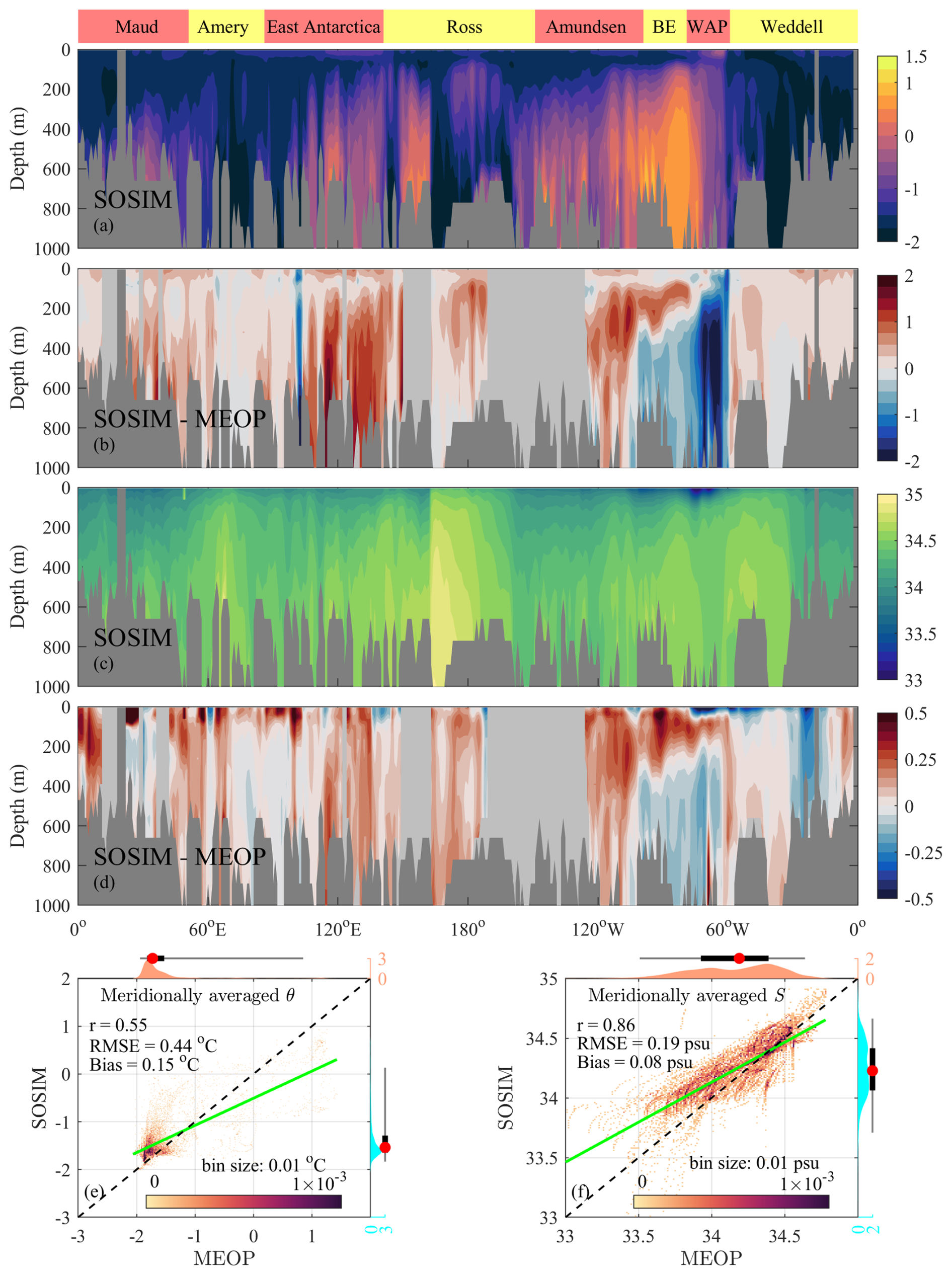
Figure 18 The vertical structure of θ (°C) and S (psu) over the continental shelf. (a) Meridionally averaged θ over the continental shelf in SOSIM. (b) The differences of SST between SOSIM and gridded MEOP (SOSIM minus MEOP). The light grey region indicates the absence of data in MEOP. (c, d) As in (a, b), but for S. (e) Statistical comparison of meridionally averaged θ over the continental shelf between SOSIM and WOA18. (f) As in (e), but for S.

The meridional mean structure of S over the Antarctic shelf is also influenced by the sea ice freezing/melting, atmospheric forcing, and salt advection (Fig. S13b). Formed through brine rejection during winter sea ice production, dense SW in the western Ross sector is characterized by particularly high S. In contrast, influenced by ice shelf basal melt and summer sea ice melting, a fresher layer spreads widely at the sea surface. In the Bellingshausen and WAP sectors, notable CDW intrusion contributes to high S at mid and deep depths, with S exceeding 34.5 psu. The halocline depth across the West Antarctic shelf also exhibits a distinct zonal gradient, being deeper in the Amundsen sector and shallower toward the WAP sector.

Compared to the MEOP climatology, SOSIM captures the broad meridional mean structure of S and its zonal variability across the Antarctic shelf (Fig. 18c), though regional biases are present (Fig. 18d). Although SOSIM shows a saline bias in the surface layer relative to MEOP, our assessment still focuses on the mid and deep layers due to the sparse spatiotemporal coverage of the MEOP observations in the highly variable surface layer. SOSIM reproduces the saline dense SW in the deep layer in the Ross regime (Fig. 18c), even showing a local saline bias there (Fig. 18d). SOSIM does not reproduce the relatively high S in the deep layers in the WAP and Bellingshausen sectors, with fresh biases of $\sim -\mathrm{0.1}$ psu that are consistent with the underestimated CDW intrusion in these regions. Meanwhile, saline biases of up to ∼0.25 psu are found at mid depths in the Bellingshausen and Amundsen sectors, which are related to the overly shallow halocline in SOSIM.

The performance of SOSIM in the meridionally averaged θ is weaker (Fig. 18e), with a moderate correlation (r=0.55), an RMSE of 0.44 °C, and a warm mean bias of 0.15 °C. The regression slope is again lower than that of the 1:1 line. The PDF peak of SOSIM ($\sim -\mathrm{1.6}$ °C) shifts toward warmer θ compared to MEOP ($\sim -\mathrm{1.8}$ °C), yet their main distributions largely overlap within the range from $\sim -\mathrm{2}$ to $\sim -\mathrm{1}$ °C. In contrast, the meridionally averaged S is simulated with high skill (Fig. 18f), evidenced by a strong correlation (r=0.86), an RMSE of 0.19 psu, and a small mean bias of 0.08 psu. The PDFs of both SOSIM and MEOP cover an identical range from ∼33.50 to ∼34.75 psu. The PDF of MEOP has a dominant peak at ∼34.38 psu and a secondary one at ∼33.98 psu, while the PDF of SOSIM shows two peaks of comparable magnitude at ∼34.10 and ∼34.42 psu.

3.6 Potential temperature, salinity, and currents over the continental slope

The ASC/ASF encircles the Antarctic continental shelf and plays an important role in regulating the exchanges of heat, salt, and mass between the Southern Ocean and shelf seas. Three typical ASC/ASF were classified by Thompson et al. (2018), including the Warm Shelf, Dense Shelf, and Fresh Shelf regimes. The Warm Shelf regime features an eastward-flowing ASC associated with the southern boundary of the ACC. Over the continental slope, the pycnocline shoals onshore and extends onto the continental shelf, with this weakened ASF allowing CDW to access the shelf. The bottom-intensified westward-flowing ASC has been identified over the Dense Shelf regime. Beneath a V-shaped ASF, cold and dense SW flows into the deep ocean in the bottom layer, and the pycnocline deepens onshore over the lower slope and shoals again over the shelf break. MCDW is able to access the shelf along the V-shaped isopycnals. The Fresh Shelf regime is characterized by a surface-intensified westward-flowing ASC. SW is separated from warm MCDW offshore by a sharp ASF, with the pycnocline intersecting the seafloor on the upper slope.

To evaluate the simulated ASC/ASF in SOSIM, three representative transects were selected, each located within a distinct dynamical regime (blue lines in Fig. 5b). The transects in the Bellingshausen, Ross, and Maud sectors represent typical characteristics of the Warm Shelf, Dense Shelf, and Fresh Shelf regimes, respectively. Given that the assessment encompasses θ, S, and velocity fields, Y2025 and SOSE are introduced to evaluate the ASF and ASC, respectively.

The meridional structure of θ along the three selected transects from Y2025 reveals the typical characteristics of ASC/ASF in different dynamical regimes (Fig. S14 in the Supplement). In the Bellingshausen sector, the isopycnals associated with the warm CDW extend directly onto the continental shelf, allowing CDW to flood the deep shelf with θ reaching up to ∼1.2 °C. In the Ross sector, MCDW upwells from the deep ocean onto the shelf; however, due to the presence of cold and dense SW overflows, the isopycnals shoal again southward across the shelf break, resulting in MCDW occupying mid-depth layers over the shelf. In contrast, along the transect in the Maud sector, the isopycnals associated with MCDW in the deep ocean intersect the seafloor on the continental slope, which largely suppresses the onshore intrusion of MCDW. Nevertheless, a limited amount of MCDW still crosses the shelf break along this transect.

SOSIM reproduces the three typical thermal structures of the ASF across different regimes, although there are some differences from Y2025. In the Bellingshausen sector, SOSIM captures the onshore intrusion of CDW and its presence in the deep layer on the continental shelf (Fig. 19a), yet the simulated CDW intrusion is weaker than in Y2025 (Fig. 19b), with a maximal θ of ∼0.5 °C. These cold biases result from CDW that approaches the slope in SOSIM being not as warm as in Y2025. In the Ross Sea sector, SOSIM reproduces the shoaling of isopycnals and associated onshore transport of MCDW into mid-shelf depths (Fig. 19d), with a warm bias at mid-depth at the thermocline depth (Fig. 19e). In the Maud sector, compared to Y2025, SOSIM simulates colder shelf waters and a more pronounced southward and downward tilt of isopycnals over the slope, which more effectively restricts the onshore intrusion of MCDW (Fig. 19g and h). In both the Bellingshausen and Ross sectors, since the thermocline depths in SOSIM are shallower than in Y2025 (Fig. 19a and d), warm biases are present in the subsurface layer on the continental slope (Fig. 19b and e). In the Maud sector, the more inclined isopycnals in SOSIM lead to cold biases near the shelf break, with the coldest bias less than −1 °C (Fig. 19h).

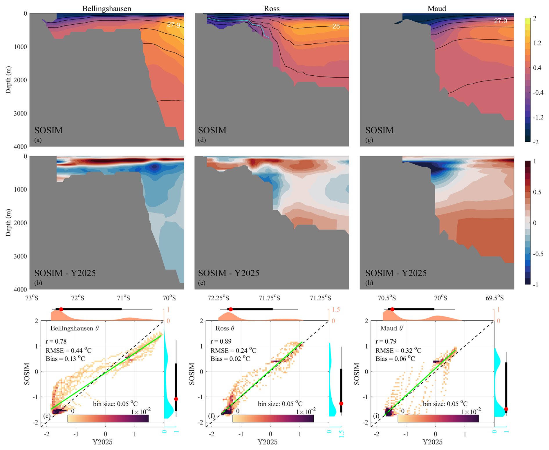
Figure 19 The meridional structure of θ (°C) along the selected transects (blue lines in Fig. 5b) perpendicular to the continental slope. (a) Climatological θ along the selected transect in the Bellingshausen sector in SOSIM. Black lines denote σ₀ (kg m⁻³) in contour intervals of 0.1 kg m⁻³. (b) The differences of θ between SOSIM and Y2025 (SOSIM minus Y2025). (c) Statistical comparison of θ along the transect in the Bellingshausen sector between SOSIM and WOA18. (d–f) and (g–i) As in (a–c), but for the transects in the Ross and Maud sectors, respectively. The cyan line in (d) denotes the γⁿ contour of 28.27 kg m⁻³.

SOSIM demonstrates consistently high performance in reproducing the observed hydrographic structures over the continental slope. The simulated statistical characteristics of θ over the slope show very good agreement with observations from Y2025 across all sectors (lower panels in Fig. 19). In the Bellingshausen sector (Fig. 19c), the correlation between SOSIM and Y2025 is strong (r=0.78), with an RMSE of 0.44 °C and a slight warm mean bias of 0.13 °C. The regression slope is slightly lower than unity. The PDFs of both SOSIM and Y2025 show a bimodal structure, with similar primary peaks at $\sim -\mathrm{1.5}$ and $\sim -\mathrm{1.6}$ °C, respectively. The secondary peak in SOSIM (∼0.5 °C) is somehow cooler than that in the observations (∼0.8 °C). SOSIM performs best in the Ross sector (Fig. 19f), showing a high correlation (r=0.89), low error (RMSE=0.24 °C), and minimal mean bias (0.02 °C). The regression line is nearly parallel to the 1:1 line, and the bimodal PDF structures of SOSIM and observations are remarkably similar, sharing similar primary ($\sim -\mathrm{1.6}$ °C in SOSIM and $\sim -\mathrm{1.4}$ °C in Y2025) and secondary (∼0.4 °C in SOSIM and ∼0.5 °C in Y2025) peaks. In the Maud sector (Fig. 19i), the performance of SOSIM remains strong (r=0.79), with an RMSE of 0.32 °C and a negligible mean bias. The PDFs are again bimodal with matching primary peaks ($\sim -\mathrm{1.6}$ °C), though the secondary peak in SOSIM (∼0.4 °C) is warmer than that observed (∼0.1 °C).

The three selected transects from Y2025 show the distinct meridional structures of S in different ASC/ASF regimes (Fig. S15 in the Supplement). In the Bellingshausen sector, strong ice shelf basal melting results in a fresh surface layer, while the intrusion of saline CDW at depth leads to high S exceeding 34.7 psu on the continental shelf. In the Ross sector, intense sea ice production in the Ross Sea and Terra Nova Bay polynyas leads to the formation of the most saline SW that is subsequently transported offshore toward the slope. As a result, the transect is characterized by high S SW over the upper slope, with maximum values reaching ∼34.8 psu. As dense SW descends the continental slope, it contributes to the uplift of isopycnals and reinforces the characteristics of the Dense Shelf regime. In the Maud sector, owing to the limited intrusion of MCDW and the absence of strong sea ice formation, the transect is characterized by relatively fresh SW, consistent with a typical Fresh Shelf regime.

SOSIM captures the typical haline structures of the ASF across three different regimes, though there are also some differences compared to Y2025. In the Bellingshausen sector, SOSIM captures the saline CDW intrusion onto the continental shelf at depth (Fig. 20a), yet S in the deep layer is not as high as in Y2025 due to the relatively fresher CDW originating in the deep ocean offshore (Fig. 20b). Meanwhile, a shallower halocline in SOSIM leads to saline biases in the subsurface layer. In the Ross Sea sector, SOSIM reproduces the saline dense SW that flows from the inner shelf to the shelf break, consistent with Y2025 (Fig. 20d and e). Yet, the absence of the γⁿ contour of 28.27 kg m⁻³ in the deep ocean shows the drift of AABW in SOSIM (Fig. 20d). In the Maud sector, SOSIM simulates fresher SW than in Y2025, with pronounced fresh biases present near the shelf break (Fig. 20g and h). It is noteworthy that the bottom S along the Maud transect in Y2025 reaches up to 34.7 psu (Fig. S15c), which has not been identified in the MEOP and may represent some uncertainties in Y2025. The fresher SW and potentially stronger ASF in SOSIM are more consistent with the theoretical framework of a Fresh Shelf regime as described by Thompson et al. (2018), suggesting that SOSIM may still have a good representation of the haline structure over the Fresh Shelf regime (Fig. 20g).

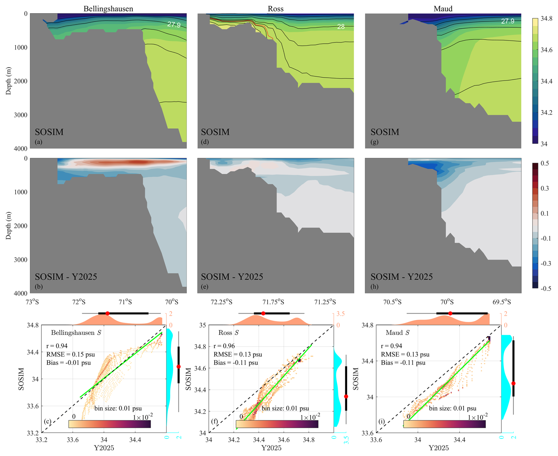
Figure 20 As in Fig. 19, but for S (psu), with the red line denoting the γⁿ contour of 28.27 kg m⁻³.

The simulated statistical characteristics of S over the slope agree well with observations across all sectors (lower panels in Fig. 20). In the Bellingshausen sector (Fig. 20c), SOSIM shows a very high correlation (r=0.94), with a low RMSE (0.15 psu) and negligible mean bias. The regression is nearly parallel to the 1:1 line. Both SOSIM and Y2025 show bimodal PDFs, yet the peaks are less pronounced in SOSIM. The primary peak in SOSIM (∼34.16 psu) is slightly saltier than that in Y2025 (∼33.98 psu), while the secondary peak in SOSIM (∼34.64 psu) is slightly fresher than that in Y2025 (∼34.71 psu). In the Ross sector (Fig. 20f), the performance of SOSIM is still very high (r=0.96, RMSE=0.13 psu), though with a negative mean bias (−0.11 psu). The bimodal structure of PDF in SOSIM is very similar to that of Y2025, with the peaks in SOSIM (∼34.22 and ∼34.66 psu) slightly fresher than in Y2025 (∼34.37 and ∼34.70 psu). In the Maud sector (Fig. 20i), SOSIM also performs well (r=0.94, RMSE=0.13 psu), with a similar negative mean bias (−0.11 psu) as in the Ross sector. While the primary PDF peaks match at ∼34.65 psu, the secondary peak in SOSIM corresponds to a fresher water mass (∼34.06 psu) compared to the observed secondary peak (∼34.25 psu).

Since the ASC generally flows along isobaths, we diagnose the flow along isobaths u_along as follows:

$$\begin{array}{}\text{(14)}& u_{\text{along}}=(u,v)\cdot \left({\displaystyle \frac{\mathrm{1}}{\left|\mathrm{\nabla }h\right|}}{\displaystyle \frac{\partial h}{\partial y}},-{\displaystyle \frac{\mathrm{1}}{\left|\mathrm{\nabla }h\right|}}{\displaystyle \frac{\partial h}{\partial x}}\right)\end{array}$$

where h is a positive value and denotes the distance from the seafloor to the rested sea surface, and ∇ is the horizontal nabla operator. The spatial structure of the u_along in SOSE is largely consistent with the classification described by Thompson et al. (2018) (Fig. S16 in the Supplement). In the Bellingshausen sector, the eastward-flowing ASC core is located over the mid-slope, associated with the southern boundary of the ACC rather than the local winds. The surface current is strong and weakens gradually with depth, with nearly negligible velocity near the seafloor. Such an eastward ASC occupies a broad zone, extending from the shelf break into the deep ocean. In the Ross sector, the westward-flowing ASC is bottom-intensified and confined to the continental slope, associated with active dense SW overflows. A relatively weak eastward current is present in the upper layer over the lower slope; however, the existence of this counterflow lacks clear observational confirmation. In addition, the γⁿ contour of 28.27 kg m⁻³ is absent in SOSE, implying that SOSE may not reproduce high S SW over the continental shelf in the Ross Sea and corresponding AABW formation over the slope. In the Maud sector, the ASC flows westward and is strongly surface-intensified, with its maximum velocity confined to the upper 100 m. The current weakens rapidly with depth and is almost absent near the bottom, associated with polar easterlies and onshore Ekman transport. Compared to the simulated ASC in ACCESS-OM2 (Huneke et al., 2022), the ASC in SOSIM also seems to be overestimated.

SOSIM demonstrates a good capability in reproducing the typical characteristics of the ASC. In the Bellingshausen sector, the eastward-flowing ASC core is identified over the mid-slope (Fig. 21a). The current is strong in the upper layer and weakens with depth, consistent with the general structure in SOSE. However, SOSIM produces a slightly weaker eastward core and a westward undercurrent over the lower slope (Fig. 21b). Notably, such a deep westward undercurrent has been observed in the Warm Shelf regime and is dynamically linked to SW exports (Thompson et al., 2020). In the Ross Sea sector, SOSIM captures the westward-flowing ASC, with a bottom intensification confined to the continental slope (Fig. 21c). In contrast to the SOSE product, SOSIM does not generate an eastward countercurrent on the slope, showing closer agreement with mooring observations (Gordon et al., 2009). Furthermore, the bottom-intensified ASC in SOSIM is stronger than in SOSE (Fig. 21d), which is likely attributable to stronger dense SW overflow in SOSIM compared to the potentially underestimated overflow in SOSE. In the Maud sector, SOSIM replicates the westward ASC, with a remarkable surface intensification (Fig. 21e). Compared to SOSE, the simulated ASC in the Maud sector weakens less rapidly with depth (Fig. 21f), associated with the more steeply inclined isopycnals (Fig. 21e). Overall, the ASC in SOSIM is generally overestimated.

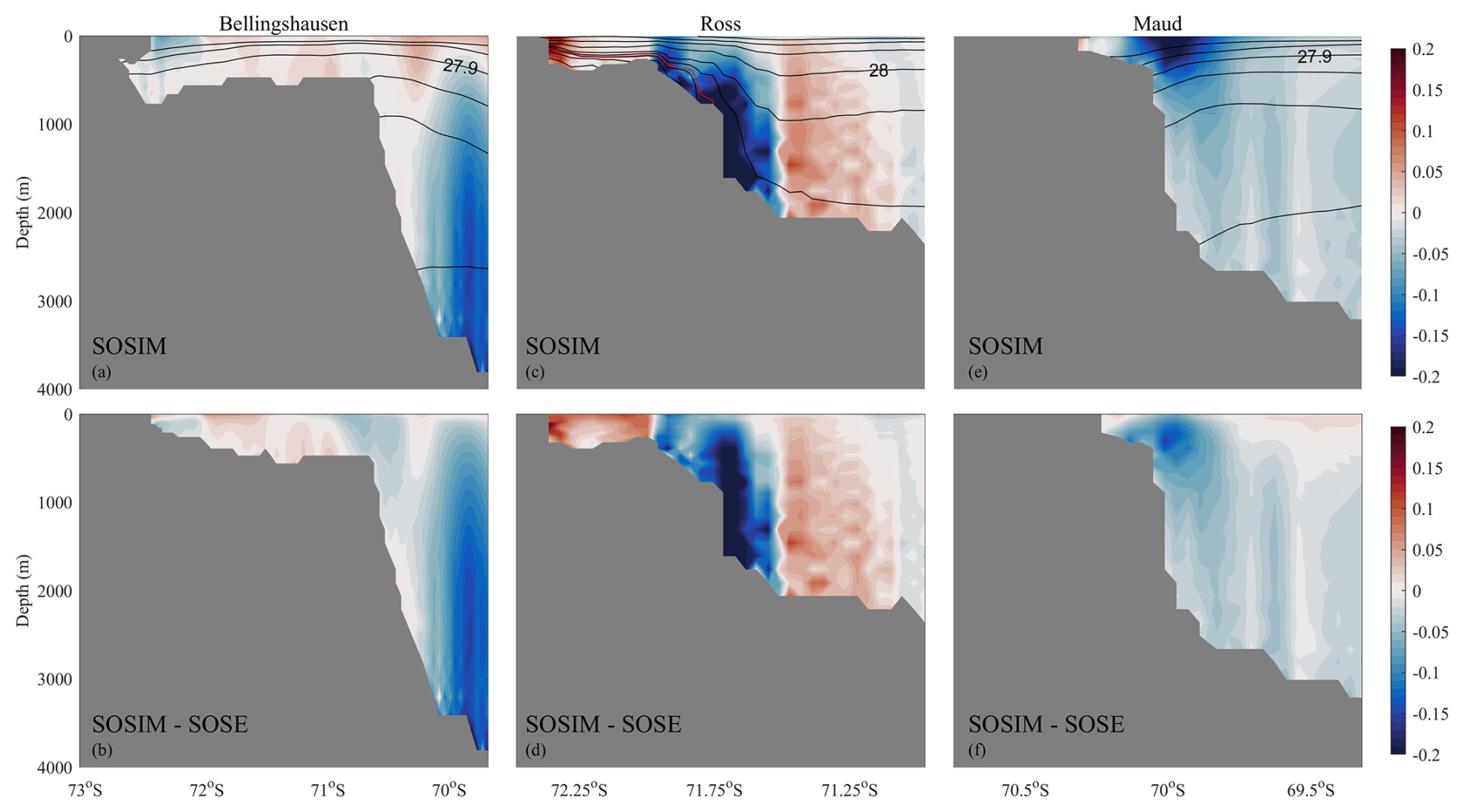
Figure 21 The meridional structure of u_along (m s⁻¹) along the selected transects (blue lines in Fig. 5b) perpendicular to the continental slope. (a) Climatological u_along along the selected transect in the Bellingshausen sector in SOSIM. Positive values indicate a current flowing to the right of the down-slope direction (i.e., a generally eastward-flowing ASC). Black lines denote σ₀ (kg m⁻³) in contour intervals of 0.1 kg m⁻³. The red line denotes the γⁿ contour of 28.27 kg m⁻³. (b) The differences of u_along between SOSIM and the SOSE (SOSIM minus the SOSE). (c, d) and (e, f) As in (a–b), but for the transects in the Ross and Maud sectors, respectively.

3.7 Sea ice

Sea ice plays an important role in regulating the sea surface heat, salt, and momentum fluxes through its seasonally contrasting influences. During the austral winter, sea ice insulates the ocean from the atmosphere and reduces further heat loss from the ocean to the cold air. In coastal polynyas, where sea ice is continuously advected away, resulting in low SIC, intense sea ice production and associated brine rejection trigger deep convection. In the austral summer, the high albedo of sea ice reflects solar radiation and suppresses rapid ocean warming. Driven by the combined atmospheric and oceanic forcing, the annual freeze-thaw cycles of sea ice are evident. The SIA/SIE expands dramatically during winter, with the ice edge advancing northward to encircle Antarctica and reaching its maximum extent in September. Conversely, the SIA/SIE retreats substantially in summer, leaving residual ice mainly confined to coastal areas, with the minimum extent occurring in February.

The SIC product from the UB depicts the spatial distributions of SIC in February and September (Fig. S17 in the Supplement), which represent the months of minimum and maximum SIA/SIE, respectively. In February, the remaining ice is largely confined to coastal regions, and the most evident retention of sea ice is present in the eastern Weddell Sea, where SIC reaches 1.0. In September, the sea ice edge extends northward notably into the Southern Ocean. In particular, the Weddell and the Ross Seas experience an extensive ice coverage that extends close to 55° S. Except within the marginal ice zone, SIC values are generally close to 1.0 across most ice-covered regions. Additionally, polynyas are also observed near the Antarctic coast, characterized as low SIC or even open water and maintained by strong katabatic winds and ocean heat fluxes.

SOSIM captures the strong seasonal cycle of SIC (upper panels in Fig. 22), yet notable biases are also evident in summer (Fig. 22b). Compared to the observation from the UB, SOSIM significantly underestimates the sea ice coverage in February. Most of the coastal sea ice melts away in the austral summer, with residual ice confined mainly to the western Weddell Sea, though even there the simulated SIC is lower than observed. In contrast, SOSIM performs better in simulating the SIC in winter (Fig. 22e). The simulated spatial distribution of SIC in September agrees well with the satellite product across much of the Southern Ocean. SOSIM reproduces the northward expansion of ice in the Weddell and Ross Seas to around 55° S, as well as the presence of coastal polynyas. The primary discrepancies in winter are found along the sea ice marginal zone, with lower SIC and a southward-biased ice edge in the South Indian sector and higher SIC in the Southern Atlantic and Southern Pacific sectors.

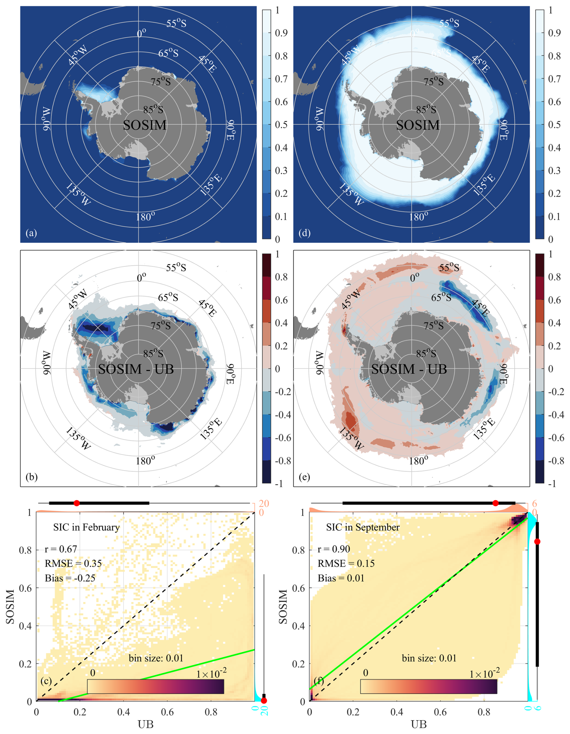
Figure 22 The spatial pattern of SIC. (a) The simulated SIC in February in SOSIM. (b) The differences of SIC between SOSIM and UB (SOSIM minus UB). (c) Statistical comparison of the SIC between SOSIM and UB. (d–f) As in (a–c), but for September.

Compared to observed sea ice from the UB, the simulated SIC in February shows a moderate correlation (r=0.67) but a substantial negative mean bias (−0.25) and a high RMSE (0.35) (Fig. 22c). The regression slope is considerably lower than that of the 1:1 line. The PDFs reveal a fundamental discrepancy. While observations from the UB show a relatively uniform distribution between 0 and 0.4, the PDF of SOSIM sharply peaks near $\mathrm{3}\times {\mathrm{10}}^{-\mathrm{3}}$ and is confined to a much narrower range from 0 to 0.1. In contrast, the performance of SOSIM in simulating the SIC in September is markedly better (Fig. 22f). The agreement between the simulated and observed SIC is very good, with a high correlation (r=0.90), low RMSE (0.15), and negligible mean bias. The regression line agrees well with the 1:1 line. The PDFs of both SOSIM and UB are remarkably similar, both exhibiting a bimodal structure with a primary peak at ∼0.95 (distributed between 0.8 and 1.0) and a secondary peak at $\sim \mathrm{1}\times {\mathrm{10}}^{-\mathrm{2}}$ (distributed between 0 and 0.1).

SOSIM demonstrates a strong capability in reproducing the observed temporal evolution and seasonal cycle of sea ice, albeit with some notable biases in summer (Fig. 23). The simulated SIA is compared to observations from both the UB (2002–2022) and the NSIDC (1979–2022) (Fig. 23a). In September, the interannual variability of the simulated SIA shows very good agreement with the observed SIA maximum. Particularly, SOSIM successfully reproduces the pronounced SIA decline from 2014 to 2016 and its subsequent recovery (Turner et al., 2017; Wang et al., 2019; Chen et al., 2025). The Pearson correlation coefficient between SOSIM and UB for the SIA in September is up to 0.91. In contrast, the simulated SIA in February is systematically lower than in both observational datasets and exhibits a reduced amplitude of interannual variability. The performance of the simulated SIE is similar to that of the SIA (Fig. 23b). Yet, while the simulated SIE in February remains negatively biased, the magnitude of the bias is smaller than that of the SIA, and its interannual variability is more comparable to observations, yielding a Pearson correlation coefficient of 0.81 with observations from the UB.

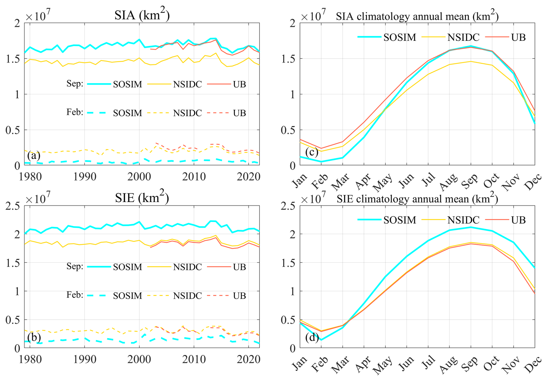
Figure 23 Time series for the assessments of sea ice. (a) The solid cyan line is the time series of the domain-integrated SIA in September, the solid orange line denotes the domain-integrated SIA in September provided by the UB, and the solid yellow line denotes the domain-integrated SIA in September provided by the NSIDC. The dashed lines are similar to the solid lines, but for February. (b) As in (a), but for the SIE. (c) The climatology annual cycle of SIA. (d) As in (c), but for the SIE.

The climatological annual cycles of the SIA and SIE show the performance of SOSIM in simulating the seasonality of sea ice (Fig. 23c and d). The simulated SIA in winter is comparable to observations from the UB, yet SOSIM underestimates the SIA in summer (Fig. 23c). Furthermore, SOSIM tends to overestimate the SIE most of the year, with the exception of the January–March period (Fig. 23d). Although such systematic biases exist, SOSIM still captures the seasonal cycle of the sea ice with remarkable fidelity, evidenced by high Pearson correlation coefficients (up to 0.99) with both observational datasets.

Based on the satellite-derived product from the UB, distinct seasonal characteristics are evident in the SIT (Fig. S18 in the Supplement). In February, the SIT in the remaining ice-covered areas is generally less than 0.3 m. The thickest sea ice is found in the Western Weddell Sea, with a maximum of ∼0.4 m. In September, a strong thickness gradient is observed in the sea ice marginal zone, where SIT decreases rapidly from 0.3 to 0 m over relatively short distances. Across the interior pack ice regions, the SIT is generally thicker than 0.4 m, with maximum values of ∼0.5 m. Conversely, thickness decreases to as low as 0.1 m in coastal polynyas. It is worth noting that satellite-derived SIT estimates are subject to relatively larger uncertainties in thick-ice regions; therefore, observations of the SIT in summer are generally considered more reliable than those in winter.

In February, since SOSIM produces a lower SIE compared to observations (Figs. 22a and 23d), the SIT is generally biased low along most of the Antarctic coastal regions (Fig. 24a and b). Yet, SOSIM produces thicker SIT in embayed regions, such as the western Weddell Sea and fjords in the WAP sector, suggesting that the convoluted coastline and enclosed bathymetry restrict the advection of sea ice and promote local ice accumulation in high-resolution models. In September, the simulated SIT shows reasonable agreement with satellite data over the open ocean, capturing the strong spatial gradients near the ice edge (Fig. 24d). Nonetheless, regional biases are also evident (Fig. 24e). SOSIM overestimates thickness in the South Atlantic and South Pacific sectors, while a negative bias occurs primarily within the marginal ice zone in the South Indian sector. On the continental shelf, the SIT in SOSIM is consistently biased higher than observed, particularly in the coastal regions where positive summer biases were identified. Given the uncertainties in satellite-derived SIT for thick ice (Huntemann et al., 2014), the simulated ice thickness in SOSIM may still be plausible despite these discrepancies.

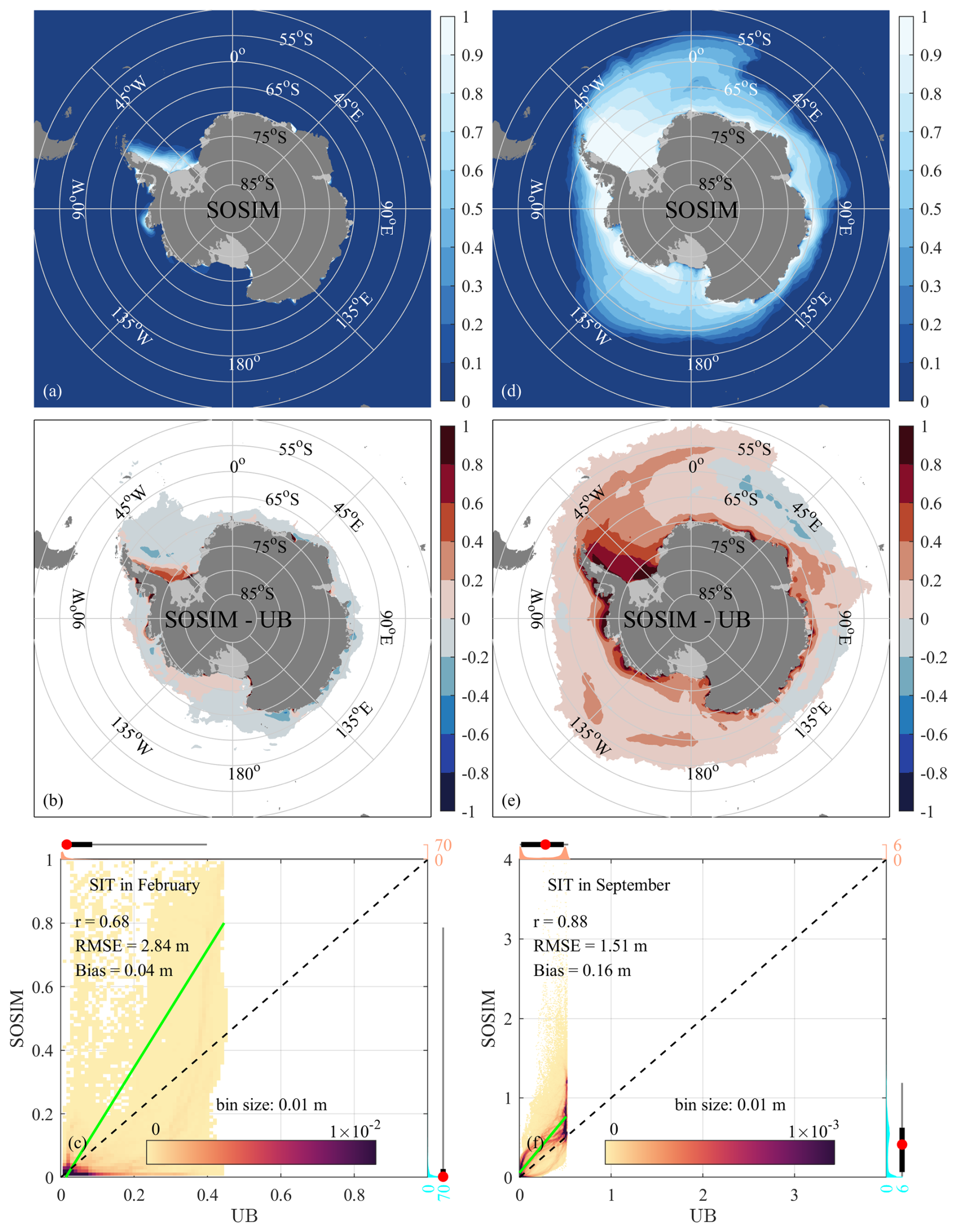
Figure 24 As in Fig. 22, but for the SIT (m).

For the SIT in February (Fig. 24c), the correlation remains moderate (r=0.68), with a low mean bias of 0.04 m, and the regression slope is higher than unity. The PDFs of both SOSIM and UB are relatively consistent, each showing a single-peaked structure near $\mathrm{5}\times {\mathrm{10}}^{-\mathrm{3}}$ m. For the SIT in September (Fig. 24f), SOSIM performs well in the correlation (r=0.88), albeit with a relatively high RMSE of 1.51 m and a slight positive mean bias of 0.16 m. The regression slope is also higher than unity. The main difference lies in the PDF shapes. Observations from the UB show two distinct peaks at $\sim \mathrm{5}\times {\mathrm{10}}^{-\mathrm{3}}$ and ∼0.5 m, whereas SOSIM produces a dominant single peak at $\sim \mathrm{5}\times {\mathrm{10}}^{-\mathrm{3}}$ m and a very subdued secondary peak at ∼0.5 m. Consequently, the simulated SIT distribution (from ∼0 to ∼1 m) is broader than observed (from ∼0 to ∼0.5 m).

Based on satellite observations from March to October, the sea ice product from the HU depicts the spatial pattern of SIP during the freezing season (March–October) by assuming that heat loss at the sea surface is all used for sea ice formation (Fig. S19 in the Supplement). Coastal polynyas are identified as the primary sites of high SIP, with maximum values typically exceeding 5 m yr⁻¹. This elevated production occurs because polynyas remain largely ice-free due to strong and persistent offshore winds that continuously transport newly formed ice away, enabling rapid and sustained ice growth at the exposed ocean surface. In contrast, SIP over the shelf regions north of the polynyas is relatively lower, likely due to the presence of more consolidated and thicker ice that insulates the ocean from the atmosphere. Compared to the inner shelf, SIP shows a moderate increase over the continental slope and adjacent deep ocean areas, consistent with enhanced SIP in the ice divergence zone (Holland and Kimura, 2016; Komatsu et al., 2025), where sea ice divergence maintains relatively thin SIT and promotes enhanced SIP. Farther north, SIP decreases toward the marginal ice zone, where it declines to zero. In accordance with the SIP estimated by the HU, we assess the simulated SIP induced by air-sea heat flux.

SOSIM captures the overall spatial distribution of SIP, with the highest production (>5 m yr⁻¹) in coastal polynya regions and lower values over the open ocean (Fig. 25a). The simulated SIP gradually declines to zero toward the marginal ice zone. However, compared quantitatively to the observational product, notable biases are also present (Fig. 25b). SOSIM systematically overestimates SIP in coastal polynyas, with positive biases exceeding 5 m yr⁻¹. These overestimates are reduced to around 1 m yr⁻¹ in open oceans, while negative biases are found in the marginal ice zone of the Indian Ocean sector and in the Weddell Sea. One potential factor contributing to the biases of nearshore SIP in SOSIM may be overestimated air-ice stress in SOSIM. This overly strengthens the offshore advection of sea ice by katabatic wind, which persistently clears coastal polynyas and allows for excessive new ice formation.

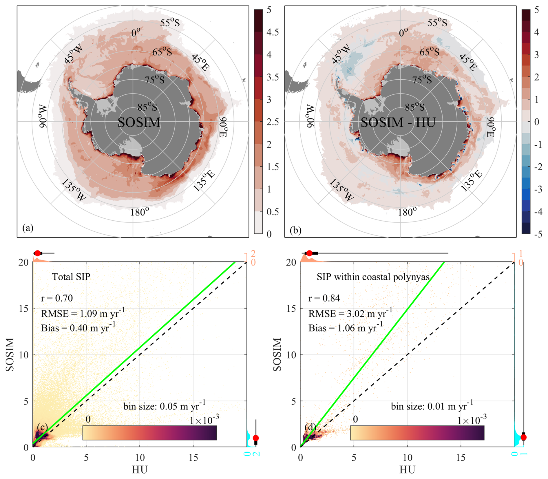
Figure 25 The spatial pattern of SIP (m yr⁻¹) during the freezing period (March–October). (a) The simulated SIP in SOSIM. (b) The differences of SIP between SOSIM and HU (SOSIM minus HU). (c) Statistical comparison of the SIP between SOSIM and HU. (d) As in (c), but for coastal polynyas.

The total SIP in SOSIM shows a good correlation (r=0.70) with observations from the HU (Fig. 25c), with a reasonable error (RMSE=1.09 m yr⁻¹) and a positive mean bias of 0.40 m yr⁻¹. The regression line is nearly parallel to the 1:1 line. Both SOSIM and observations exhibit bimodal PDFs, with a primary peak at $\sim \mathrm{1.0}\times {\mathrm{10}}^{-\mathrm{2}}$ m yr⁻¹ and a main distribution between 0 and ∼2.0 m yr⁻¹. The secondary peak in SOSIM is at a higher value (∼1.2 m yr⁻¹) than in the observations from the HU (∼0.4 m yr⁻¹). The performance of SOSIM is somewhat better in simulating the SIP over coastal polynyas (defined as SIC<0.7) (Fig. 25d), with a high correlation (r=0.84), a high RMSE (3.02 m yr⁻¹), and a positive mean bias (1.06 m yr⁻¹). The PDF structures are still somewhat dissimilar. Observations from the HU show a primary peak centered at ∼0.4 m yr⁻¹, while SOSIM generates a relatively flat distribution around the primary peak at ∼1.0 m yr⁻¹, indicating an overestimation of SIP within coastal polynyas.

3.8 Ice Shelves

Driven by ocean thermal forcing, the basal mass balance of ice shelves plays an important role in the Antarctic climate system and contributes to global sea level rise. Basal melting, particularly intense near grounding lines, is primarily induced by the intrusion of CDW or MCDW that transports heat onto the continental shelf and into sub-ice-shelf cavities. Conversely, localized basal freezing often occurs in cold cavities, contributing to the stability of large ice shelves. The spatial pattern of melting and freezing rates is closely related to ocean circulation, heat transport, and the geometry of sub-ice-shelf cavities.

The product from A2020 depicts the spatial pattern of Antarctic ice shelf basal melt rates (Fig. S20 in the Supplement). High basal melt rates exceeding 5 m yr⁻¹ are found beneath ice shelves in West Antarctica, including the WAP, Amundsen, and Bellingshausen sectors. Intense melting is also observed in the Totten Ice Shelf in East Antarctica and near the grounding zones of the Amery Ice Shelf, with melt rates exceeding 5 m yr⁻¹. In contrast, basal freezing primarily occurs in the central regions of the three largest ice shelves, namely, the Ross, Filchner-Ronne, and Amery ice shelves. Despite these localized areas of freezing, melting dominates over freezing across Antarctic ice shelves.

SOSIM captures the overall spatial pattern of ice shelf basal melt rates as depicted in the A2020 product (Fig. 26a). SOSIM reproduces high melt rates exceeding 5 m yr⁻¹ beneath ice shelves in the WAP, Amundsen, and Bellingshausen sectors. Yet, notable biases are also present in the simulated basal mass balance (Fig. 26b). SOSIM does not capture the intense melting near the grounding zone of the Amery Ice Shelf and the high melt rates observed at the Totten Ice Shelf. In addition, SOSIM fails to reproduce the basal freezing of the three largest ice shelves. The difficulty in simulating basal freezing is likely attributable to the coarse vertical resolution, which results in an overly thick oceanic boundary layer in contact with the ice shelf and artificially enhances oceanic heat flux toward the ice.

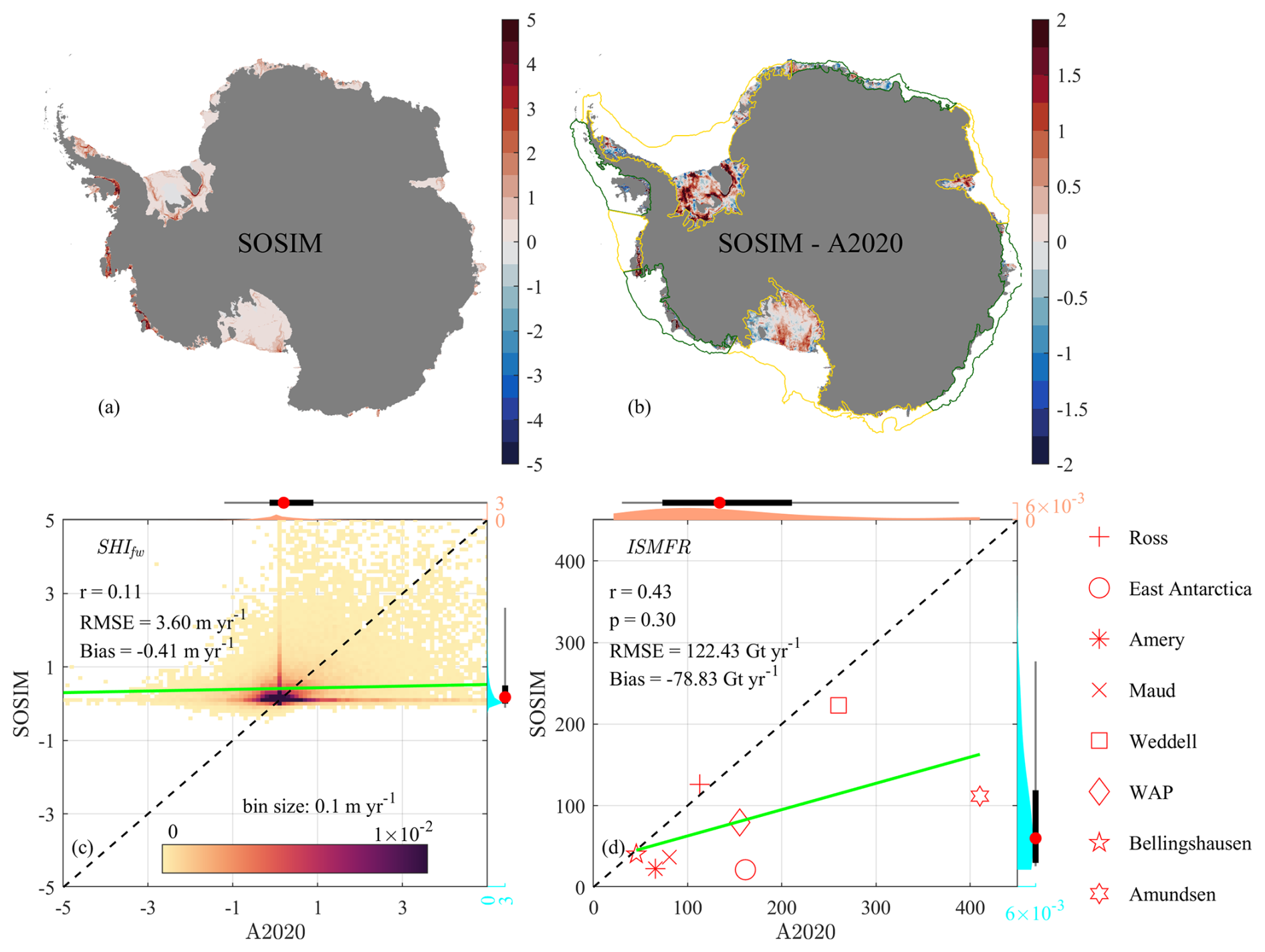
Figure 26 The annual climatology of the basal melting/freezing rate of ice shelves. (a) The observed spatial pattern of SHI_fw (m yr⁻¹) from A2020. (b) As in (a), but for SOSIM. (c) The differences of SHI_fw between SOSIM and A2020 (SOSIM minus A2020). Green lines and yellow lines denote the division of the Antarctic shelf seas (as in Fig. 5b). (d) The area-integrated ISMFR (Gt yr⁻¹) within every sector over shelf seas.

Based on the statistical comparison of ice shelf basal melt rates between SOSIM and the A2020 observational dataset, the model demonstrates limited skill in reproducing the observed patterns. For the simulated SHI_fw (Fig. 26c), SOSIM shows a very weak correlation (r=0.11) with observations from A2020, with a high RMSE of 3.6 m yr⁻¹ and a negative mean bias of −0.41 m yr⁻¹. The linear regression line is nearly horizontal, indicating a poor systematic relationship. It shows a substantial statistical overestimation for melting/freezing rates below 0.4 m yr⁻¹ and a substantial statistical underestimation for melting/freezing rates above 0.4 m yr⁻¹. The PDFs for both SOSIM and A2020 peak near 0 m yr⁻¹. However, the observed distribution of the PDF from A2020 is centered around this peak, spreading relatively evenly between −1 and 1 m yr⁻¹. In contrast, the PDF of SOSIM is strongly skewed toward positive values, with its main distribution confined between 0 and 1 m yr⁻¹, suggesting a model bias toward melting over freezing conditions at the ice shelf basal surface.

For the area-integrated ISMFR within each sector over the continental shelf (Fig. 26d), the performance of SOSIM is somewhat better but remains suboptimal, with a low correlation (r=0.43) that is not statistically significant (p=0.30). The RMSE is high (122.43 Gt yr⁻¹), and the negative mean bias is also relatively larger (−78.83 Gt yr⁻¹), indicating a systematic underestimation of the total melting/freezing flux by SOSIM. Consequently, the regression slope is lower than that of the 1:1 line. The PDFs of SOSIM and A2020 cover a similar range (from 25 to 300 Gt yr⁻¹), but the peak of SOSIM distribution (50 Gt yr⁻¹) shifts toward lower values compared to the observed peak (100 Gt yr⁻¹), consistent with the overall negative bias. Despite these biases, the relatively good agreement in the Bellingshausen, Ross, and Weddell sectors suggests the utility of SOSIM for studying ocean–ice shelf interactions in these regions.

4 Discussion

Overall, SOSIM demonstrates a reasonable ability to reproduce the observed large-scale features in the Southern Ocean. The simulated θ and S in the open ocean agree well with WOA18, particularly in the zonally averaged fields. SOSIM also captures the typical structure of the ASC/ASF in different dynamical regimes, the seasonality of the sea ice, and the general pattern of the basal mass balance of ice shelves. However, several systematic biases and limitations were found by our evaluations.

4.1 The simulated oceanic biases

One of the most notable biases in SOSIM is the underestimation of the ACC transport (Fig. 15). The simulated barotropic streamfunction shows a transport of only ∼77 Sv through the Drake Passage, significantly lower than the observed range of 134–173 Sv. This bias may be attributed to several factors. First, the proximity of the northern open boundary to the core of the ACC may restrict the full development of the current within the model domain. The prescribed open boundary conditions from ECCO2 and WOA18 may not fully represent the dynamical interactions at the northern edge. Second, the overestimation of eddy activity in SOSIM (Fig. 16), while slightly overestimating the intensity of mesoscale processes, may also lead to an excessive energy transfer from the MKE to the EKE, thereby weakening the mean flow. The underestimation of the ACC transport appears to be a common challenge in high-resolution circumpolar configurations, as noted in previous studies (Farneti et al., 2015; Kiss et al., 2020). To further understand the underestimated ACC transport, future sensitivity experiments (e.g., testing different northern open boundary configurations, horizontal resolutions, or advection schemes) would be valuable for diagnosing and potentially mitigating this bias.

Another significant bias is the warm and fresh drift in the deep and abyssal layers (Figs. 8–11), particularly in the Southern Atlantic and Southern Indian sectors. This suggests a deficiency in the representation of AABW formation and spreading in the abyssal layer (Fig. 14). Although dense SW is produced in coastal polynyas, as indicated by the overestimated SIP (Fig. 25) and water masses on the continental shelf (Figs. 17 and 18), its subsequent transformation into AABW via mixing with CDW and downslope transport may be inadequately captured (Figs. 19 and 20). The vertical resolution, while improved over predecessors like ECCO2, might still be insufficient to resolve the small-scale processes governing the dense overflows on the continental slope. Given the persistent drifts in the abyssal ocean (Fig. 7), shelf-focused applications are likely to be more robust than basin-scale abyssal trend analyses.

Furthermore, SOSIM shows contrasting biases in simulating onshore deep water intrusion (Figs. 17 and 18). The intrusion of CDW is underestimated in the Bellingshausen sector, leading to cold biases on the shelf, while a shoaled thermocline and excessive warm deep water intrusion at mid-depths in most of the remaining sectors introduce warm biases. Such regional inconsistencies may be attributed to the biases in the representation of the ASC/ASF (Figs. 19–21), the simulated water masses approaching the continental slope from deep oceans (Figs. 9 and 11), and the surface fresh and heat fluxes regulated by the sea ice evolution over the continental shelf (Figs. 22–25). Indeed, the overestimation of the ASC in SOSIM may play an important role in the simulated biases in cross-slope exchanges.

4.2 The simulated sea ice biases

SOSIM reproduces the winter SIC and SIE reasonably well but significantly underestimates summer sea ice coverage and overestimates the amplitude of the seasonal cycle for both SIA and SIE (Fig. 23). This seasonal bias is likely linked to the zero-layer thermodynamic scheme used in the sea ice model, which does not account for heat storage within the ice. This leads to an overly rapid response to atmospheric forcing, causing ice to melt too quickly in summer and form too rapidly in autumn. Despite a similar spatial pattern of the simulated SIP with observations (Fig. 25), the overestimation of SIP in coastal polynyas still shows the biases in the representation of the sea ice dynamics in response to katabatic winds.

4.3 The simulated basal melting/freezing biases of ice shelves

SOSIM captures the spatial pattern of high basal melt rates in West Antarctic ice shelves but systematically underestimates the total ice shelf mass loss and fails to reproduce the basal freezing in cold cavities (Fig. 26). These two deficiencies may result from several model limitations. First, the lack of tidal forcing in SOSIM may be a key candidate for explaining the underestimation of total ice loss, as tides are known to enhance vertical mixing and facilitate the thermal forcing available to enhance the basal melting of ice shelves (Padman et al., 2018). The absence of tidal forcing reduces the vertical mixing and heat flux towards the ice shelf base, particularly in the critical grounding zones. Second, the vertical resolution of SOSIM, even with partial cells, is still too coarse to properly resolve the turbulent ice shelf–ocean boundary layer, leading to an artificially thick boundary layer and an overestimation of the oceanic heat available for ice melting (Schodlok et al., 2016). Third, the omission of frazil ice simulation may also contribute to the absence of basal freezing (Galton-Fenzi et al., 2012; Herraiz-Borreguero et al., 2013). Consequently, SOSIM cannot properly reproduce the basal freezing of ice shelves in cold cavities (e.g., the cavities beneath the Ross and Filchner-Ronne ice shelves).

4.4 Potential uncertainties in observational and reanalysis data sets

Our comprehensive evaluation of SOSIM quantifies the deviations of model results from observations and reanalysis. However, discrepancies between SOSIM and benchmark data may stem not only from model deficiencies but also from the limitations in the observation and reanalysis datasets in the data-sparse Southern Ocean.

A notable discrepancy between SOSIM and SOSE is revealed in the simulated structure of the ASC in the Bellingshausen and Ross sectors (Fig. 21). While SOSE depicts an eastward-flowing ASC throughout the water column in the Bellingshausen sector, SOSIM reproduces a westward-flowing undercurrent on the continental slope. This westward undercurrent appears to be a model artifact but is supported by observational evidence. Based on full-depth in situ measurements in the Bellingshausen Sea, Thompson et al. (2020) identified a westward bottom boundary current beneath the eastward surface flow. In addition, an eastward ASC in the Ross sector in SOSE has not been observed. The remarkable agreement between SOSIM and in situ observations underscores the capability of SOSIM to capture complex oceanic processes in this region, implying the potential uncertainties of reanalysis data sets in regions of limited observations.

Compared to the observed SIT in winter, the significant positive bias in the simulated SIT (Fig. 24) may be partially attributed to known uncertainties in the satellite products. The SIT from the UB is derived from both SMOS and SMAP L-band microwave sensors (Paţilea et al., 2019), and such a SMOS/SMAP-based product is specifically optimized for estimating thin ice thickness (typically <0.5 m) (Huntemann et al., 2014). A constraint of the L-band radiometry is the saturation of the brightness temperature signal for thicker ice, leading to rapidly increasing uncertainty and a low sensitivity for thicker ice. In winter, the SMOS/SMAP retrieval likely underestimates the SIT in regions of consolidated pack ice. The discrepancy between the simulated and observed SIT in winter may not indicate a model bias, but rather represents a physical reality that lies beyond the reliable detection range of this specific satellite product.

4.5 Advantages of SOSIM

Beyond the specific biases discussed above, we also highlight the advantages and innovations embodied in the SOSIM configuration, which establish it as a valuable tool for investigations focused on the shelf seas around Antarctica.

First, SOSIM represents one of the state-of-the-art eddy-resolving COSIMs. By integrating the coupled ocean–sea ice–ice shelf models, SOSIM simultaneously simulates the evolution of the dynamically and thermodynamically active ocean, sea ice, and static ice shelves within a consistent high-resolution framework. The inclusion of interactive ice shelf cavities, with thermodynamic melting and freezing at the ice–ocean interface following a friction-velocity-dependent parameterization, allows for in-depth investigations of the feedbacks between oceanic heat transport and the ice shelf mass balance, which is a critical process for projecting sea-level rise. Meanwhile, since SOSIM is built on a z-coordinate framework, this configuration provides a distinct advantage in topographic representation. Compared to terrain-following sigma-coordinate models, which often require significant smoothing of steep slopes to avoid pressure gradient errors over the steep ice shelf fronts and the continental slope, the z-coordinate allows for a more accurate representation of the bedrock and ice draft from the RTopo-2 dataset. Therefore, SOSIM enables a more faithful simulation of the dynamical influences of topography on oceanic currents (St-Laurent et al., 2013; Liu et al., 2022).

Second, SOSIM has good capability in simulating the dynamics over the Antarctic continental shelf and slope. Over the continental shelf, SOSIM reliably reproduces the properties of bottom water, and it also captures the meridionally averaged hydrographic structures, with a good correlation with the MEOP dataset (Figs. 17 and 18). SOSIM accurately reproduces the distinct three-dimensional structures of the ASC/ASF across the Warm, Dense, and Fresh Shelf regimes (Figs. 19–21). Statistical comparisons along key transects show very high correlations for both θ and S (Figs. 19 and 20), underscoring the fidelity of SOSIM in representing these typical features of cross-slope exchanges.

Third, SOSIM shows robust performance in simulating the seasonal cycle and interannual variability of sea ice. While biases still exist in summer, SOSIM performs well in simulating the winter sea ice state. The spatial pattern of SIC in winter is captured with remarkable accuracy (Fig. 22), and SOSIM faithfully reproduces the observed interannual variability of the SIE in winter, including the pronounced decline from 2014 to 2016 and its subsequent recovery (Fig. 23). The high Pearson correlation coefficient (0.99) for the climatological annual cycle of both SIC and SIE with observations also confirms its skill in simulating the fundamental seasonality of the sea ice cover.

Finally, the development of SOSIM is designed with long-term applications and community utility in mind. It serves as the dynamical core for the next generation of the Southern Ocean Ice Prediction System in China (Zhao et al., 2024). The configuration, including its use of widely adopted forcing datasets (ERA5) and topography (RTopo-2), enhances its reproducibility and potential for future intercomparison studies. The quantitative evaluation presented in this study provides a benchmark for its current capabilities and a baseline for measuring future improvements.

Table 1 A summary of the performance of SOSIM.

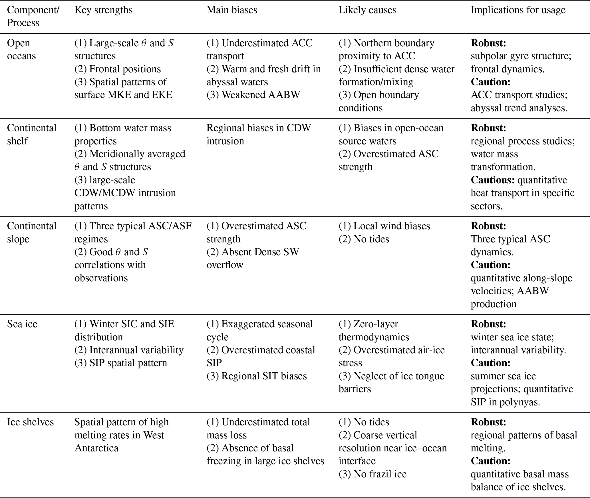
Overall, the principal attributes of SOSIM lie in its combination of a high-circumpolar-resolution z-coordinate framework, coupling of core components, and its design as a foundation for both operational prediction and fundamental research. These features make it an innovative model for advancing our understanding of the complex interactions within the Antarctic climate system.

To provide a concise summary of the performance of SOSIM, we synthesize our evaluation in Table 1. By outlining the primary strengths, major biases, the likely causes of these biases, and the practical implications for future applications, Table 1 intends to clearly show the regimes and processes that are robust in SOSIM, as well as those where caution is warranted or further development is still necessary.

4.6 Future improvements

Building upon the demonstrated capabilities and identified limitations of SOSIM, we propose several priority directions for its future development. These enhancements are aimed at addressing the systematic biases discussed above.

Both the horizontal and vertical resolutions could be further refined. A further refinement of the horizontal resolution to ∼1 km over the continental slope and shelf regions would allow SOSIM to explicitly resolve mesoscale eddies and finer-scale dynamics that are crucial for cross-slope and cross-shelf heat and salt transports. Such an enhancement is expected to significantly improve the representation of eddy-driven exchanges and their impact on water mass transformations on the shelf. Increasing the vertical resolution, especially in the upper ocean and near the ice–ocean interface (Aguiar et al., 2025), would better represent key physical processes, such as the dense overflows on the continental slope and the basal mass balance of ice shelves.

The configuration of sea ice could be further improved. First, implementing a more comprehensive sea ice model with multi-layer thermodynamics (Winton, 2000) would likely suppress the exaggerated seasonal cycle of SIA and SIE by allowing the heat storage in sea ice. Second, calibrating the sea ice dynamics parameterization, particularly the air-ice stress, may be useful to mitigate the overestimation of SIP in coastal polynyas. Third, incorporating more accurate representations of coastal ice tongues and grounded icebergs into the SOSIM bathymetry is crucial. These features act as natural barriers that significantly influence the sea ice drift, the opening of polynyas, and the associated SIP (Ohshima et al., 2013).

The spin-up strategy requires optimization. The significant drift in the integrated HC, SC, and particularly the ISMFR during the initial decades of the interannual forcing period indicates that the year 1979, which is used repetitively for spin-up, does not represent a climatically neutral state, leading to a subsequent adjustment drift when interannual atmospheric forcing was applied. Therefore, spinning up the model under a carefully selected neutral year (Stewart et al., 2020) would suppress the initial drift and enhance the stability and reliability of SOSIM for long-term simulations.

COSIMs could benefit a lot from including more components. First, the inclusion of tidal forcing is important, as it is expected to enhance the vertical mixing, strengthen cross-slope exchanges, promote AABW formation, and increase the basal melting rate of ice shelves, thereby addressing corresponding key biases simultaneously. We therefore highlight the inclusion of tidal forcing as a priority avenue for future development of SOSIM. Second, the development towards a fully coupled atmosphere–ocean–sea ice–ice sheet model would allow for a more realistic representation of air–ocean–ice interactions, which are crucial for simulating climate variability and changes in the Southern Ocean.

In addition, the ongoing enhancement of observational networks, alongside more sophisticated reanalysis products that assimilate a growing suite of in situ and satellite measurements, will provide increasingly robust benchmarks. Such improved observational and reanalysis datasets will be invaluable for the future calibration, validation, and improvement of all COSIMs, helping to clarify model biases and leading to a more accurate representation of the Southern Ocean system.

5 Concluding remarks

In this study, we have presented the configuration and a comprehensive evaluation of SOSIM v1.0, a high-resolution circumpolar coupled ocean–sea ice–ice shelf model based on the MITgcm. SOSIM is designed to simulate the complex interactions among the ocean, sea ice, and ice shelves in the Southern Ocean, with a horizontal resolution of ∼5 km and 70 vertical levels.

A comprehensive evaluation against a suite of observational and reanalysis datasets demonstrates that SOSIM is capable of reproducing the fundamental hydrographic characteristics of the Southern Ocean. SOSIM successfully captures the large-scale hydrographic structures in the deep ocean, the CDW/MCDW intrusion onto the continental shelf, the structure of the ASC/ASF in different dynamic regimes, the seasonal cycle of sea ice, and the general spatial pattern of basal melting rates of ice shelves around Antarctica.

Meanwhile, our evaluation also identifies several key biases. The model underestimates the transport of the ACC and shows a warm and fresh drift in the abyssal ocean, indicating a deficiency in the representation of AABW formation. The simulated sea ice exhibits an exaggerated seasonal cycle, with a significant underestimation of summer coverage. The total basal mass loss of Antarctic ice shelves is also underestimated.

In summary, SOSIM v1.0 provides a useful tool for investigating mesoscale processes, cross-slope exchanges, and ocean–sea ice–ice shelf interactions in the Southern Ocean. The model configuration and evaluation presented in this study pave the way for future developments, including the incorporation of tidal forcing, refined horizontal and vertical resolutions, and more sophisticated parameterizations. Furthermore, SOSIM is poised to serve as the backbone for the next-generation Southern Ocean Ice Prediction System in China (Zhao et al., 2024), which is based on an ocean–sea ice coupled model with a horizontal resolution of 18 km. Overall, SOSIM will benefit from continued development and community engagement.