sedExnerFoam 2412: a 3D Exner-based sediment transport and morphodynamics model

Predicting the complex interplay between flow hydrodynamics, sediment transport, and morphological evolution is a key challenge in hydraulic and coastal engineering. This paper presents an open-source numerical model for sediment transport and morphological evolution called sedExnerFoam. Implemented in the C++ multi-physics simulation toolkit OpenFOAM, the model combines high-resolution hydrodynamics with a transport equation for suspended sediment concentration, as well as a morphological evolution module based on the Exner equation. The sediment bed is one of the computational domain's boundaries, and its geometry varies over time. In turn, the evolution of the bed position affects the hydrodynamics through mesh deformation. Following a thorough description of the model, a series of benchmark tests is presented to evaluate its performance and demonstrate its capabilities. These benchmarks consist of a set of simplified simulations designed to validate each model component independently. These include a turbulent suspension case in an equilibrium channel, a case in which the flow transitions from a rigid starved bed to an erodible bed, becoming progressively laden with suspended sediments, and an idealized dune migration scenario that is decoupled from flow hydrodynamics. Finally, two deposition tests validate the model's mass conservation capability and highlight the avalanche mechanism that prevents excessive bed slope steepness. After the model has been validated, an application to the migration of a single dune under the influence of a steady flow is presented. Incorporating spatial bedload flux saturation is essential for achieving stable simulations and quantitative comparisons with experimental data in this application. The work presented in this manuscript represents a significant initial step in the development of a fully operational open-source model. Nevertheless, many improvements are still required. The article lists guidelines for future developments to inform future work.

1 Introduction

The transport of sediments and morphodynamics, that is, the evolution of the sedimentary bed, is a complex physical problem involving many processes related to fluid mechanics, through the action of water on sedimentary particles, and solid mechanics when avalanches occur due to gravity. A coupling instability mechanism between fluid flow and bed evolution can also lead to the formation of bedforms, typically ripples or dunes (Kennedy, 1963; Charru et al., 2013). These bedforms alter the bed roughness and create a feedback loop on the fluid flow, which can result in a significant increase in flood risk in rivers or estuaries (van der Sande et al., 2025; Hu et al., 2024). Therefore, morphodynamics models are essential tools for hydraulic engineers working on coastal, river, and estuarine systems, as they can be used to analyze erosion phenomena and assess the impact of human constructions, such as bridges, dams, and renewable marine energy production systems (e.g., wind and tidal turbines).

The twentieth century saw the development of analytical models (Hjelmfelt and Lenau, 1970) and one-dimensional (1D) numerical models (Cunge et al., 1980; Goutal and Maurel, 2002) for the study of hydraulic and morphodynamic phenomena. In the 1980s and 1990s, two-dimensional (2D), depth-integrated, and quasi-tridimensional numerical models emerged, primarily in the fluvial domain (Hervouet, 1999). Since the early 2000s, several three-dimensional (3D) models have been developed, including for coastal areas. Some are open-source, such as openTELEMAC (Benoit et al., 2002), ROMS/CROCO (Warner et al., 2008; Marchesiello et al., 2015), and DELFT3D (Lesser et al., 2004), while others are proprietary, such as MIKE (Warren and Bach, 1992). Most of these models are adapted to flows on “large spatial and temporal scales”, and are often based on the use of sigma coordinates in the vertical direction. This does not allow for the integration of obstacles such as bridge piers or wind turbine masts (Hervouet, 2007; Lesser et al., 2004). Another important approximation made in these models lies in the parametrization of the boundary layer: the first computational node above the bed is located in the logarithmic layer. Therefore, these models are not particularly suitable for simulating interactions between morphodynamics and fluid flow around structures laid on the bottom, or for simulating processes such as scouring or bed instability, including the formation of ripples and dunes.

A new generation of 3D models based on emergent computational fluid dynamics (CFD) (Liu and García, 2008; Jacobsen, 2011; Baykal et al., 2015), allows for a finer resolution of flow and turbulence, particularly in the boundary layer and in the wake zones around structures. These models are based on the Arbitrary Lagrangian-Eulerian (ALE) approach, which handles the evolution of the bed boundary and the deformation of the associated volume mesh. To our knowledge, there is no open-source model of this type. While other approaches are possible, such as the immersed boundary method (IBM) (Song et al., 2022) or multiphase approaches (Chauchat et al., 2017; Nagel et al., 2020; Gilletta et al., 2024), these are too computationally expensive for engineering applications. The ALE method, therefore, seems to be the best compromise. As part of a collaboration between the University of Grenoble Alpes (CNRS, Grenoble INP, and INRAE) and the engineering company ARTELIA Group, an open-source model is being developed within the C++ library OpenFOAM^® (v2412) (Jasak et al., 2007). This model, named sedExnerFoam (Renaud et al., 2025), is an ALE-based numerical framework developed to support a wide range of hydraulic engineering applications. While its development was initially motivated by the need to study scour around hydraulic structures, the model is intended as a more general tool for simulating sediment–flow interactions, such as studying the formation and migration of bedforms in channels, assessing sediment deposition and erosion patterns in rivers, and analyzing sediment accumulation in reservoirs.

Non-uniform flow situations in sediment transport, including flow around hydraulic structures, channel contractions or expansions, and regions of rapidly varying bed morphology, require a fine local resolution to accurately capture the resulting flow features. To address this, the model relies on a CFD approach to solve the hydrodynamics and the excess of shear stress exerted on the sediment bed. This enables the study of various problems that cannot be simulated with depth-integrated models or models that rely on boundary layer parametrization. For instance, the migration of steep bedforms with flow separation occurring at their lee side due to the adverse pressure gradient (van der Sande et al., 2025) (see Fig. 1), or scour around a bridge pile and the horseshoe vortex which is the driving mechanism causing erosion upstream of the pile (Chiew and Melville, 1987; Roulund et al., 2005), or jet driven scour downstream of a sluice gate (Chatterjee et al., 1994; Martino et al., 2019).

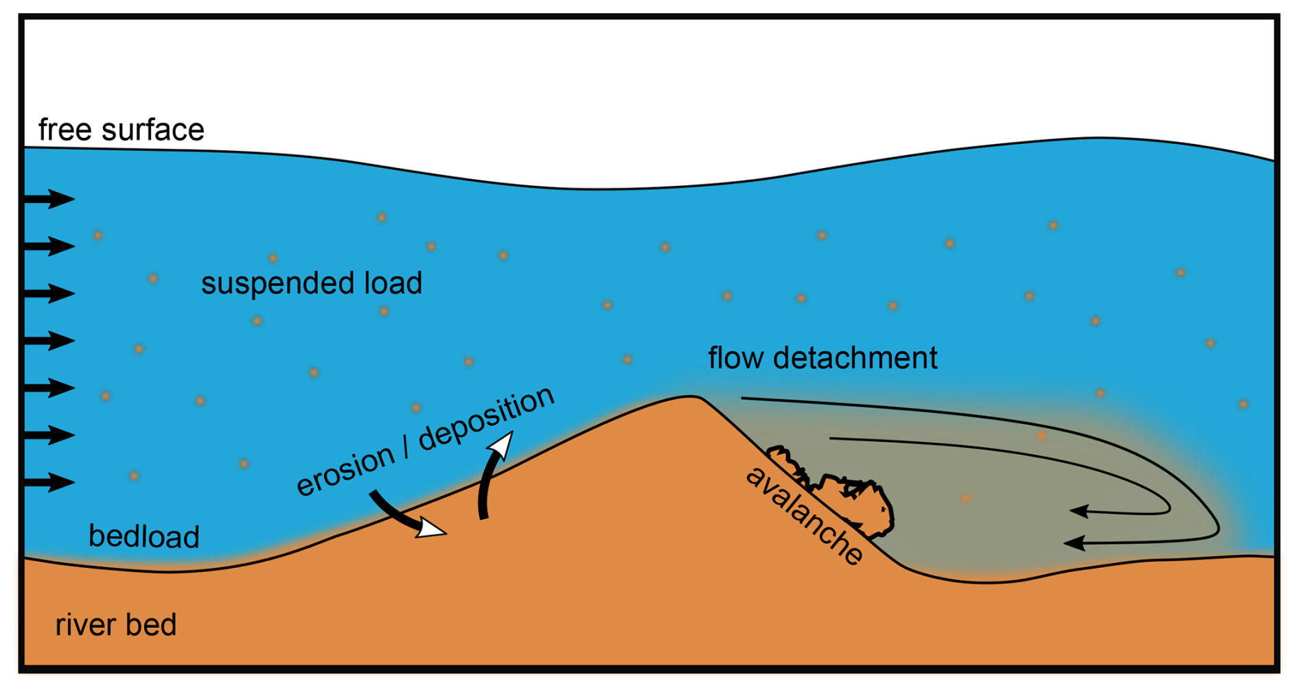
Figure 1 Schematic representation of the flow above a riverbed and the main sediment transport processes involved.

After presenting the mathematical formulation of sedExnerFoam in Sect. 2 and the modeling approaches for hydrodynamics, turbulence, and sediment transport closures, several key numerical aspects are discussed in Sect. 3, with particular emphasis on the treatment of the Exner equation. It is followed, in Sect. 4, by the model validation against a series of academic benchmarks, which consist of simple test cases designed to isolate individual components of the model and validate them separately against analytical solutions or experimental data. The validation suite includes simulations of idealized dune migration, sediment suspension under steady flow conditions, both in and out of equilibrium, as well as two sediment deposition scenarios. Finally, in Sect. 5, the model’s capabilities are demonstrated through the simulation of an isolated dune migrating over a rigid bed under steady flow conditions. The numerical results reproduce a stationary migration regime, characterized by the dune moving at a constant velocity while maintaining its shape throughout the migration process. The conclusion provides a summary of the present work and a discussion of the current limitations of the model, as well as possible future improvements.

2 Mathematical description

Sediment transport can be divided into two distinct modes: suspended load and bedload. Empirical formulas are used to estimate erosion and deposition fluxes between the riverbed and the water column, as well as the amount of sediment entrained in the bedload layer. This section provides a comprehensive overview of the model's components, beginning with hydrodynamics in Sect. 2.1, turbulence modeling in Sect. 2.2, and suspended-sediment transport in Sect. 2.3. It then introduces the Exner equation, which governs the evolution of the bed morphology. The various closure relations used to estimate the threshold of motion and bedload flux are described, together with the avalanche model and the treatment of bedload flux saturation. Finally, the coupling between the suspended load and the sediment bed is detailed through an erosion–deposition formulation based on the classical reference concentration.

2.1 Hydrodynamics

The fluid motion is governed by the incompressible, filtered Navier–Stokes equations:

$$\begin{array}{}\text{(1)}& \begin{array}{rl}{\displaystyle \frac{\partial \mathit{u}}{\partial t}}+\mathrm{\nabla }.(\mathit{u}\otimes \mathit{u})& =-{\displaystyle \frac{\mathrm{1}}{{\mathit{\rho }}_{\mathrm{f}}}}\mathrm{\nabla }p+\mathit{g}+\mathrm{\nabla }.(\mathrm{2}\mathit{\nu }\mathbf{S}+{\mathit{\tau }}_{\mathrm{f}}),\\ & \mathrm{\nabla }.\mathit{u}=\mathrm{0},\end{array}\end{array}$$

where the operator ⊗ is the dyadic product, u the fluid velocity, p the fluid pressure, g the gravitational acceleration, ρ_f the fluid density, ν the fluid kinematic viscosity, and $\mathbf{S}=\frac{\mathrm{1}}{\mathrm{2}}[\mathrm{\nabla }\mathit{u}+(\mathrm{\nabla }\mathit{u}{)}^T]$ is the strain rate tensor. τ_f is a tensor which definition depends on the type of filter used. It can either be the opposite of the specific Reynolds stress tensor to run Reynolds Averaged Simulations (RAS), a subgrid scale stress tensor when performing Large Eddies Simulations (LES), or the null tensor for laminar simulations or Direct Numerical Simulations (DNS). The model takes full advantage of the wide range of options provided by OpenFOAM, and the type of filtering applied to Eq. (1) can be freely selected by the user. In this study, however, the numerical simulations are limited to either laminar cases (with no filtering of the Navier–Stokes equations) or unsteady RAS simulations.

At this stage of model development, no feedback of the suspended load on the hydrodynamics is considered, i.e. the fluid density ρ_f is assumed to be constant, an assumption appropriate for dilute suspensions where density effects and particle drag are negligible.

2.2 Turbulence modeling

As stated previously, in the case of RAS filtering, the tensor τ_f in Eq. (1) is equal to the opposite of the specific Reynolds stress tensor ${\mathit{\tau }}_{\mathrm{f}}=-〈{\mathit{u}}^{\mathbf{\prime }}\otimes {\mathit{u}}^{\mathbf{\prime }}〉$, with 〈〉 the Reynolds operator and u^′ the fluctuating velocity field. A total of 6 additional unknowns (the velocity fluctuation correlations) are introduced in the system of equations by the use of the Reynolds stress tensor. The system as such is undetermined and the classical Boussinesq assumption is used as a closure. It expresses the Reynolds stress tensor as a function of the eddy viscosity ν_t and $k=\frac{\mathrm{1}}{\mathrm{2}}〈{\mathit{u}}^{\mathbf{\prime }}.{\mathit{u}}^{\mathbf{\prime }}〉$, the turbulent kinetic energy (TKE):

$$\begin{array}{}\text{(2)}& {\mathit{\tau }}_{\mathrm{f}}=\mathrm{2}{\mathit{\nu }}_{\mathrm{t}}\mathbf{S}-{\displaystyle \frac{\mathrm{2}}{\mathrm{3}}}k{\mathbf{I}}_{\mathrm{3}},\end{array}$$

where I₃ is the identity matrix. Then, a turbulence model is used to compute ν_t. OpenFOAM offers multiple turbulence models to users, many of which are two-equation models based on k and either ϵ or ω, the rate of dissipation of TKE, and the specific rate of dissipation of TKE, respectively. A transport equation is then solved for each variable.

Of the various turbulence models available for the RAS approach in OpenFOAM (k−ϵ, k−ω, RNG k−ϵ …), only the well-known k−ω Shear Stress Transport (SST) model introduced by Menter (1994) is employed in this study, although the other turbulence models available in OpenFOAM are also compatible with the solver. The choice of this model was motivated by its capability to simulate both free shear flows and boundary layers, as well as its accuracy in capturing flow separation caused by adverse pressure gradients. The k−ω SST consists of a combination of two other classical turbulence models, the k−ϵ (Launder and Spalding, 1983) and the k−ω (Wilcox, 1998) models. The aim is to take the best out of those two models. Indeed, the k−ϵ model is known to perform well for free shear flows but exhibits poor accuracy in the presence of adverse pressure gradients, rendering it unsuitable for flows involving boundary layer separation. Conversely, the k−ω model is better suited for capturing flows with adverse pressure gradients and boundary layers, but it is less efficient than the k−ϵ for simulating free shear flows in regions outside the range of influence of the solid boundaries (e.g., rigid walls, sediment bed). The k−ω SST model transitions between the two models using blending functions that take the distance to the nearest wall as input. In the version implemented in OpenFOAM, the eddy viscosity ν_t is expressed as follows:

$$\begin{array}{}\text{(3)}& {\mathit{\nu }}_{\mathrm{t}}=a_{\mathrm{1}}{\displaystyle \frac{k}{max(a_{\mathrm{1}}\mathit{\omega },b_{\mathrm{1}}{F}_{\mathrm{23}}\Vert \mathbf{S}\Vert )}},\end{array}$$

where F₂₃=F₂F₃ is the product of two blending functions (F₂ and F₃) and $\Vert \mathbf{S}\Vert =\sqrt{\mathrm{2}\mathbf{S}:\mathbf{S}}$ is a scalar measure of the strain rate tensor, with : the double inner product defined as $\mathbf{S}:\mathbf{S}=\mathrm{tr}\left({\mathbf{SS}}^T\right)$, where tr is the trace operator. The temporal evolutions of k and ω are described by two transport equations:

$$\begin{array}{}\text{(4)}& {\displaystyle \frac{\partial k}{\partial t}}+\mathit{u}.\mathrm{\nabla }k=\stackrel{\mathrm{̃}}{P}-{\mathit{\beta }}_{*}k\mathit{\omega }+\mathrm{\nabla }.\left(\right(\mathit{\nu }+{\mathit{\alpha }}_k{\mathit{\nu }}_{\mathrm{t}}\left)\mathrm{\nabla }k\right),\text{(5)}& {\displaystyle }\begin{array}{rl}{\displaystyle \frac{\partial \mathit{\omega }}{\partial t}}+\mathit{u}.\mathrm{\nabla }\mathit{\omega }& ={\displaystyle \frac{\mathit{\gamma }}{{\mathit{\nu }}_{\mathrm{t}}}}P-\mathit{\beta }{\mathit{\omega }}^{\mathrm{2}}+\mathrm{\nabla }\left(\right(\mathit{\nu }+{\mathit{\alpha }}_{\mathit{\omega }}{\mathit{\nu }}_{\mathrm{t}}\left)\mathrm{\nabla }\mathit{\omega }\right)\\ & +\mathrm{2}(\mathrm{1}-F_{\mathrm{1}}){\mathit{\alpha }}_{\mathit{\omega }\mathrm{2}}{\displaystyle \frac{\mathrm{1}}{\mathit{\omega }}}\mathrm{\nabla }k.\mathrm{\nabla }\mathit{\omega }\end{array}\end{array}$$

where F₁ is another blending function. The production term P is defined as $P={\mathit{\nu }}_{\mathrm{t}}\mathrm{\nabla }\mathit{u}:[\mathrm{\nabla }\mathit{u}+(\mathrm{\nabla }\mathit{u}{)}^T]$. In the equation for k (Eq. 4), a limiter is applied on the production rate:

$$\begin{array}{}\text{(6)}& \stackrel{\mathrm{̃}}{P}=min\left(P,c_{\mathrm{1}}{\mathit{\beta }}_{*}k\mathit{\omega }\right).\end{array}$$

The different blending functions and constants of the model are detailed in Appendix B.

2.3 Suspended sediment transport

In sedExnerFoam, the suspended load is described by the suspended sediment volume fraction $c_{\mathrm{s}}=V_{\mathrm{s}}/(V_{\mathrm{s}}+V_{\mathrm{f}})$ where V_s and V_f stand for the volume of sediment and the volume of fluid, respectively. The evolution of c_s in space and time is governed by an advection-diffusion equation:

$$\begin{array}{}\text{(7)}& {\displaystyle \frac{\partial c_{\mathrm{s}}}{\partial t}}+\mathrm{\nabla }.\left[\right(\mathit{u}+{\mathit{w}}_{\mathrm{s}}\left)c_{\mathrm{s}}\right]=\mathrm{\nabla }.\left({\mathit{ϵ}}_{\mathrm{s}}\mathrm{\nabla }{c}_{\mathrm{s}}\right),\end{array}$$

where w_s is the sediment settling velocity and ϵ_s is the turbulent diffusivity for the suspended sediment. It is expressed as the ratio of the turbulent eddy viscosity and the Schmidt number σ_c as ${\mathit{ϵ}}_{\mathrm{s}}={\mathit{\nu }}_{\mathrm{t}}/{\mathit{\sigma }}_{\mathrm{c}}$. The possibility of using an additional diffusivity ϵ_w in near-bed areas is discussed in Sect. 2.4.3. The suspended sediment concentration is supposed to behave as a passive scalar being transported with the flow and settling due to the effect of gravity. The settling velocity is computed as follows:

$$\begin{array}{}\text{(8)}& {\mathit{w}}_{\mathrm{s}}=w_{\mathrm{s}}^{\mathrm{0}}{F}_{\mathrm{h}}\left(c_{\mathrm{s}}\right){\mathit{e}}_{\mathrm{g}},\end{array}$$

where $w_{\mathrm{s}}^{\mathrm{0}}$ is the terminal sediment settling velocity of a single particle in a quiescent fluid, ${\mathit{e}}_{\mathrm{g}}=\mathit{g}/\left|\mathit{g}\right|$ is a unit vector oriented with gravity, and F_h is a hindrance function that takes values between 0 and 1 and is a decreasing function of c_s. It represents the effect of particles hindering each other as they fall, leading to a drop in their settling velocity when c_s increases (Richardson and Zaki, 1954). The terminal settling velocity is estimated using empirical formulations that either explicitly predict the settling velocity or implicitly determine it by computing the drag coefficient C_D and solving the force balance between drag, buoyancy, and weight. In the present model, all available formulations take the dimensionless diameter D_* (van Rijn, 1984) as an input, defined as follows:

$$\begin{array}{}\text{(9)}& D_{*}=d({\displaystyle \frac{(s-\mathrm{1})g}{{\mathit{\nu }}^{\mathrm{2}}}}{)}^{\mathrm{1}/\mathrm{3}},\end{array}$$

where d is the grain size, $s={\mathit{\rho }}_{\mathrm{s}}/{\mathit{\rho }}_{\mathrm{f}}$ the density ratio, and ρ_s and ρ_f are the density of the sediment and the fluid, respectively.

The values adopted for the Schmidt σ_c number have remained a topic of debate to this day, with no consensus yet reached. van Rijn (1984) proposed a formula to estimate σ_c from the sediment settling velocity and the friction velocity u_*:

$$\begin{array}{}\text{(10)}& {\mathit{\sigma }}_{\mathrm{c}}={\displaystyle \frac{\mathrm{1}}{\mathrm{1}+\mathrm{2}{\left(\frac{{\displaystyle }{w}_{\mathrm{s}}}{{\displaystyle }{u}_{*}}\right)}^{\mathrm{2}}}},\text{for}\mathrm{0.1}<{\displaystyle \frac{w_{\mathrm{s}}}{u_{*}}}<\mathrm{1}.\end{array}$$

This yields a Schmidt number smaller than one, which corresponds to suspended sediment being dispersed more effectively than momentum is mixed by turbulence. This can be explained by the fact that turbulent diffusion is not the only mechanism responsible for sediment dispersion; additional processes, such as particle collisions, particle inertia, and lift forces, can also enhance sediment diffusivity. Because these mechanisms are not accounted for in this classical approach, the Schmidt number is generally treated as a tuning parameter. In this model, the Schmidt number is treated as constant, with the preceding equation (Eq. 10) serving as a useful guideline for choosing its value.

The final key aspect of this approach is the enforcement of the bed boundary condition, i.e., the exchange of mass between the sediment bed and the suspended load. This topic is discussed in Sect. 2.4.3, which addresses erosion and deposition rates.

2.4 Bedload and Morphodynamics

Sediment transport modeling seeks to quantify how bedforms and channel morphology evolve under fluid flow. The section begins with the Exner equation description, which links bed elevation changes to sediment-flux divergence, followed by the motion threshold and bedload transport formulations that describe the onset and rate of particle motion. Slope-driven avalanching and bedload saturation further constrain near-bed dynamics, while erosion and deposition terms associated with suspended load exchange complete the framework for capturing morphodynamic evolution.

2.4.1 Exner equation

The morphological evolution of a granular bed in a wide range of sediment transport problems is modeled by the so-called Exner equation (Exner, 1920):

$$\begin{array}{}\text{(11)}& (\mathrm{1}-{\mathit{\lambda }}_{\mathrm{s}}){\displaystyle \frac{\partial z_{\mathrm{b}}}{\partial t}}+{\mathrm{\nabla }}_H.{\mathit{q}}_{\mathrm{b}}=D-E,\end{array}$$

where z_b is the bed elevation, λ_s is the porosity of the granular material, which is linked to the maximum possible sediment volume fraction $c_{\mathrm{s}}^{\max }=\mathrm{1}-{\mathit{\lambda }}_{\mathrm{s}}$. The bedload flux q_b is the specific flux of sediment transported along the bed per unit width. It is computed from the bed shear stress using an empirical formula. D and E are respectively the deposition and erosion rates; they are the terms through which sediment is exchanged between the bed and the water column. The Exner equation is a 2D equation and is thus solved after applying a 2D plane projection on all variables. The operator ∇_H stands for the divergence operator on this projected plane.

2.4.2 Bedload modeling

Sediment transport initiates when the bed shear stress τ_b exceeds a critical value, referred to as the motion threshold and expressed in dimensionless form by the Shields number $\mathit{\theta }=\left|{\mathit{\tau }}_{\mathrm{b}}\right|/({\mathit{\rho }}_{\mathrm{s}}-{\mathit{\rho }}_{\mathrm{f}})gd$ (Shields, 1936). The corresponding critical value is known as the critical Shields number θ_c. This threshold depends on fluid and sediment properties as well as on the local bed slope. For a flat bed, the critical Shields number, denoted as ${\mathit{\theta }}_{\mathrm{c}}^{\mathrm{0}}$, can be estimated using empirical formulations, many of which are based on the dimensionless sediment particle diameter D_*, such as the one proposed by Soulsby and Whitehouse (1997):

$$\begin{array}{}\text{(12)}& {\mathit{\theta }}_{\mathrm{c}}^{\mathrm{0}}={\displaystyle \frac{\mathrm{0.3}}{\mathrm{1}+\mathrm{1.2}{D}_{*}}}+\mathrm{0.055}(\mathrm{1}-e^{-\mathrm{0.02}{D}_{*}}).\end{array}$$

Determining the threshold of motion remains challenging due to the absence of a universal definition. Depending on the criterion adopted, such as initial grain displacement, sustained motion, or measurable sediment transport, different threshold values may be obtained. Moreover, the influence of bed slope requires additional corrections. The effect of local bed slope is incorporated through a correction to the critical Shields number proposed by Fredsoe and Deigaard (1992):

$$\begin{array}{}\text{(13)}& \begin{array}{rl}{\displaystyle \frac{{\mathit{\theta }}_{\mathrm{c}}}{{\mathit{\theta }}_{\mathrm{c}}^{\mathrm{0}}}}& =\cos \left({\mathit{\beta }}_{\mathrm{s}}\right)\sqrt{\mathrm{1}-{\displaystyle \frac{{\sin }^{\mathrm{2}}\left({\mathit{\alpha }}_{\mathrm{s}}\right){\tan }^{\mathrm{2}}\left({\mathit{\beta }}_{\mathrm{s}}\right)}{{\mathit{\mu }}_{\mathrm{s}}^{\mathrm{2}}}}}\\ & -{\displaystyle \frac{\cos \left({\mathit{\alpha }}_{\mathrm{s}}\right)\sin \left({\mathit{\beta }}_{\mathrm{s}}\right)}{{\mathit{\mu }}_{\mathrm{s}}}},\end{array}\end{array}$$

where β_s is the angle of the bed slope and α_s the angle between the steepest slope direction and the direction of the shear. The coefficient of static friction μ_s is linked to the angle of repose of the granular material β_r through tan (β_r)=μ_s.

Relationships between the Shields number and the dimensionless bedload flux ${\mathit{\varphi }}_{\mathrm{b}}=\left|{\mathit{q}}_{\mathrm{b}}\right|/\sqrt{(s-\mathrm{1})g{d}^{\mathrm{3}}}$ have been widely investigated (Einstein, 1942; Meyer-Peter and Müller, 1948; Van Rijn, 1984), leading to the development of numerous empirical formulations. Many commonly used expressions (Meyer-Peter and Müller, 1948; Nielsen, 1992; Ribberink, 1998) take the following form:

$$\begin{array}{}\text{(14)}& {\mathit{\varphi }}_{\mathrm{b}}\propto {\mathit{\theta }}^a\mathit{\varpi }(\mathit{\theta }-{\mathit{\theta }}_{\mathrm{c}}{)}^b,\end{array}$$

with a and b, two real positive coefficients and ϖ the threshold function so that $\mathit{\varpi }(\mathit{\theta }-{\mathit{\theta }}_{\mathrm{c}})=\mathit{\theta }-{\mathit{\theta }}_{\mathrm{c}}$ if θ>θ_c and 0 else. In this work, the bedload flux q_b is aligned with the bed shear stress.

In addition to transport driven by bed shear stress, sediment can also be mobilized through local avalanche processes when the bed slope exceeds the angle of repose of the granular material. If not taken into account, unrealistic slopes could appear in the numerical solution or even shock situations, which could trigger numerical instabilities in the model. Marieu et al. (2008) proposed a model based on an iterative procedure to redistribute the excess of sediment locally until the bed slope does not exceed the granular material angle of repose. Such a procedure has been successfully tested in other works (Zhou, 2017). In sedExnerFoam, however, the avalanche is modeled with an additional bedload term q_av inspired from Duran Vinent et al. (2019):

$$\begin{array}{}\text{(15)}& \left|{\mathit{q}}_{\mathrm{av}}\right|=q_{\mathrm{av}}^{\mathrm{0}}{\displaystyle \frac{\mathit{\varpi }\left[\tanh \right(\tan \left({\mathit{\beta }}_{\mathrm{s}}\right))-\tanh (\tan \left({\mathit{\beta }}_{\mathrm{r}}\right)\left)\right]}{\mathrm{1}-\tanh \left(\tan \right({\mathit{\beta }}_{\mathrm{r}}\left)\right)}}.\end{array}$$

with $q_{\mathrm{av}}^{\mathrm{0}}$ is a positive constant. It corresponds to the maximum possible additional bedload flux due to the avalanche. This avalanche flux is oriented toward the steepest slope direction. One benefit of this formulation is that it enables slopes to exceed the angle of repose in the event of competition between bedload flux due to bed shear stress and that due to gravitational acceleration.

One last aspect, which is often neglected when modeling sediment transport in water but is widely used in aeolian transport, is the saturation of the bedload flux. The adjustment of q_b toward its saturated value q_sat is commonly expressed in 1D (Charru, 2006; Charru et al., 2013), however, in this work, the following 2D formulation is proposed:

$$\begin{array}{}\text{(16)}& T_{\mathrm{sat}}{\displaystyle \frac{\partial {\mathit{q}}_{\mathrm{b}}}{\partial t}}+L_{\mathrm{sat}}{\mathrm{\nabla }}_H.\left({\displaystyle \frac{{\mathit{q}}_{\mathrm{sat}}}{\Vert {\mathit{q}}_{\mathrm{sat}}\Vert }}\otimes {\mathit{q}}_{\mathrm{b}}\right)={\mathit{q}}_{\mathrm{sat}}-{\mathit{q}}_{\mathrm{b}}\end{array}$$

where q_sat is the saturated flux, T_sat the saturation time, and L_sat the saturation length. When taking the saturation into account, the saturated flux q_sat is computed from the bed shear stress (see Eq. 14) and the bedload flux q_b is the solution of Eq. (16). Similar to the Exner equation, the saturation equation is solved on a horizontal plane after projection.

2.4.3 Erosion and deposition rates

As mentioned earlier, modeling erosion and deposition fluxes represents one of the main challenges in classical sediment transport models. Many sediment transport experiments in straight flumes have been conducted to study the relation between the flow and the rate at which particles are eroded from the bed to the water column. In his work, van Rijn (1984) studied the case of sediment transport in a straight channel under equilibrium conditions and proposed an empirical formula to compute a reference concentration $c_{\mathrm{b}}^{*}$ at a certain reference distance from the bed, the so-called reference level $\mathit{\delta }{z}_{\mathrm{b}}^{*}$:

$$\begin{array}{}\text{(17)}& c_{\mathrm{b}}^{*}=\mathrm{0.015}{\displaystyle \frac{d}{\mathit{\delta }{z}_{\mathrm{b}}^{*}}}{\displaystyle \frac{(\mathit{\theta }/{\mathit{\theta }}_{\mathrm{c}}-\mathrm{1}{)}^{\mathrm{3}/\mathrm{2}}}{(D_{*}{)}^{\mathrm{0.3}}}}.\end{array}$$

The reference concentration corresponds to the concentration observed at a distance $\mathit{\delta }{z}_{\mathrm{b}}^{*}$ from the bed under equilibrium conditions.

This development has been adopted in many sediment transport models, which define the boundary condition $c_{\mathrm{s}}\left(\mathit{\delta }{z}_{\mathrm{b}}^{*}\right)=c_{\mathrm{b}}^{*}$ based on the assumption of equilibrium at the reference level. The boundary condition, however, may not be valid in cases where this local equilibrium assumption is violated. It was adapted by Celik and Rodi (1988) to accommodate non-equilibrium conditions. The erosion rate is written $E=w_{\mathrm{s}}{c}_{\mathrm{b}}^{*}$ and the deposition rate D=w_sc_b, with c_b, a sediment concentration value computed from the values in the neighboring cells, which is detailed later on. The erosion rate is assumed equal to its equilibrium value, while deposition depends only on the concentration in the first cells above the bed. If $c_{\mathrm{b}}>c_{\mathrm{b}}^{*}$, then suspended sediment gets deposited on the bed, and when $c_{\mathrm{b}}<c_{\mathrm{b}}^{*}$, sediment gets eroded from the bed and suspended in the water column. The equilibrium occurs when $c_{\mathrm{b}}=c_{\mathrm{b}}^{*}$.

One difficulty lies in prescribing the reference concentration at the reference level, which is located at some distance above the bed boundary. Large-scale sediment transport models avoid this difficulty by not meshing the region located between the sediment bed and the reference level. The downfall of this method is that the flow near the bed is not solved and needs to be modeled, typically leading to bad hydrodynamics in highly non-uniform flow regions, such as near obstacles. In order to maintain a good hydrodynamics resolution, Jacobsen (2011) developed a model relying on a different mesh for the hydrodynamics and for the suspended load. The bottom boundary of the mesh for the suspended load was located at the reference level, whereas the mesh for the hydrodynamics presented cells in between the sediment bed and the reference level. In sedExnerFoam, the choice to use a single mesh was made primarily for practical reasons, to simplify the operation of the model by avoiding the use of two different meshes and by allowing all boundary conditions to be applied directly at the bed interface.

As stated previously, the deposition and erosion fluxes are computed as suggested by Celik and Rodi (1988). The erosion E is computed at the reference level $\mathit{\delta }{z}_{\mathrm{b}}^{*}=k_{\mathrm{s}}$, the Nikuradse equivalent roughness height (k_s=2.5 d), using Eq. (17) and a limiter so that $c_{\mathrm{b}}^{*}$ is not exceeding a value $c_{\mathrm{b},\max }^{*}$, typically equal to half the maximum possible sediment volume fraction. The limiter ensures that $c_{\mathrm{b}}^{*}$ remains physically realistic when the bed shear stress is high (see Eq. 17). Amoudry et al. (2005) used a maximum possible reference concentration $c_{\mathrm{b},\max }^{*}=\mathrm{0.3}$ which is close to the value of 0.32 suggested by Engelund and Fredsøe (1976). The computed reference concentration is then extrapolated at the height of the first cell center above the sediment bed boundary z₁, using the formula suggested by Fang and Rodi (2003):

$$\begin{array}{}\text{(18)}& c_{\mathrm{b}\mathrm{1}}^{*}=min\left(c_{\mathrm{b}}^{*}{e}^{-\frac{w_{\mathrm{s}\mathrm{1}}}{{\mathit{ϵ}}_{\mathrm{s}\mathrm{1}}}\left(z_{\mathrm{1}}-\mathit{\delta }{z}_{\mathrm{b}}^{*}\right)},c_{\mathrm{b},\max }^{*}\right),\end{array}$$

where $c_{\mathrm{b}\mathrm{1}}^{*}$ is the reference concentration extrapolated at the height z₁. w_s1 and ϵ_s1 stand for the settling velocity and the sediment turbulent diffusivity values at the center of the first cell above the sediment bed located at a height z₁. The expression of $c_{\mathrm{b}\mathrm{1}}^{*}$ is obtained by considering a local equilibrium in a small region above the bed and assuming ϵ_s and w_s to be uniform between the reference level $\mathit{\delta }{z}_{\mathrm{b}}^{*}$ and the center of the first cell above the bed. The deposition and erosion are then computed at the first cell center and not on the bed boundary, leading to D=w_sc₁. The total erosion/deposition rate is then estimated as:

$$\begin{array}{}\text{(19)}& D-E=w_{\mathrm{s}\mathrm{1}}(c_{\mathrm{1}}-c_{\mathrm{b}\mathrm{1}}^{*}).\end{array}$$

This flux is prescribed as a boundary condition for the suspended-load transport (Eq. 7). With this approach, the same computational mesh can be employed for both suspended-load and hydrodynamic calculations, allowing for fine resolution near the sediment bed. It should be noted that the various formulations for $c_{\mathrm{b}}^{*}$ found in the literature are empirical in nature and are derived primarily from measurements conducted in straight-channel flow experiments. Their applicability outside of such configurations, particularly in the vicinity of obstacles that disturb the flow, should therefore be treated with caution.

To address difficulties in suspending material from the bed to the water column under fine grid resolution and low roughness Reynolds number conditions $k_{\mathrm{s}}^{+}=\frac{k_{\mathrm{s}}{u}_{*}}{\mathit{\nu }}$, an additional near-bed diffusivity for suspended sediment ϵ_w was introduced in the model. In the smooth and intermediate roughness regimes, the eddy viscosity vanishes within a thin layer near the bed. When the mesh resolution is sufficiently fine such that the first cells lie within this layer, the eroded sediment tends to remain confined to these cells rather than being transported upward into the water column. The additional diffusivity introduced for suspended sediment is defined as follows:

$$\begin{array}{}\text{(20)}& {\displaystyle \frac{{\mathit{ϵ}}_w}{\mathit{\nu }}}={\displaystyle \frac{{\mathit{ϵ}}_w^{\mathrm{0}}}{\mathrm{2}}}\left(\mathrm{1}-\tanh \left({\mathit{\xi }}_w{\displaystyle \frac{z-k_{\mathrm{s}}}{k_{\mathrm{s}}}}\right)\right).\end{array}$$

It can be interpreted as the dispersion resulting from particle collisions, which is not accounted for in Eq. (7) but plays a role locally in the near-bed region, where the solid volume fraction can be significant. This term allows particles to reach an elevation above the viscous sublayer, where they can be entrained by turbulent eddies and transported upward into the water column. However, when the flow is hydraulically rough ($k_{\mathrm{s}}^{+}\ge \mathrm{90}$), turbulence penetrates down to the bed, and the use of ϵ_w is no longer necessary. The coefficients ${\mathit{ϵ}}_w^{\mathrm{0}}$ and ξ_w are both set to 5 by default.

3 Numerical implementation

The numerical implementation of sedExnerFoam is based on the finite volume method (FVM) and developed within the OpenFOAM^® (v2412) framework. The development originated from the existing solver pimpleFoam, which is designed for incompressible transient flow simulations and employs the PIMPLE algorithm for pressure-velocity coupling. This section outlines the key numerical features of the model, its operating sequence, and the numerical methods employed, with particular attention given to the treatment of the Exner equation. Finally, the case structure is presented, including all necessary files and the modeling options available to users.

3.1 Code implementation

The Navier-Stokes equations (Eq. 1) and the transport equation for suspended load (Eq. 7) are both solved using the finite volume method. The computational domain is discretized into a multitude of polyhedral control volumes over which the partial differential equations are integrated. The Exner equation, however, is solved over a surface (the sediment bed) using the finite area method (FAM). FAM is an adaptation of the finite volume methods on a surface curved in 3D space. It was initially developed by Tukovic and Jasak (2008) for the numerical study of the transport of a surfactant at the interface between two fluids and has since then been successfully applied to other problems, such as dense-flow avalanches (Rauter and Kowalski, 2024). In the present model, the finite area mesh is coupled with the volumetric mesh patch representing the sediment bed, such that the finite area mesh coincides with the bed boundary of the finite volume mesh. This approach ensures seamless interaction between flow and sediment transport without the need for multiple meshes. The discretization of the partial differential equations using the finite area method was originally developed to account for surface curvature; however, curvature effects are not considered in the present treatment of bed morphology evolution. Accordingly, the Exner equation is solved on a plane projected normal to the gravity vector g.

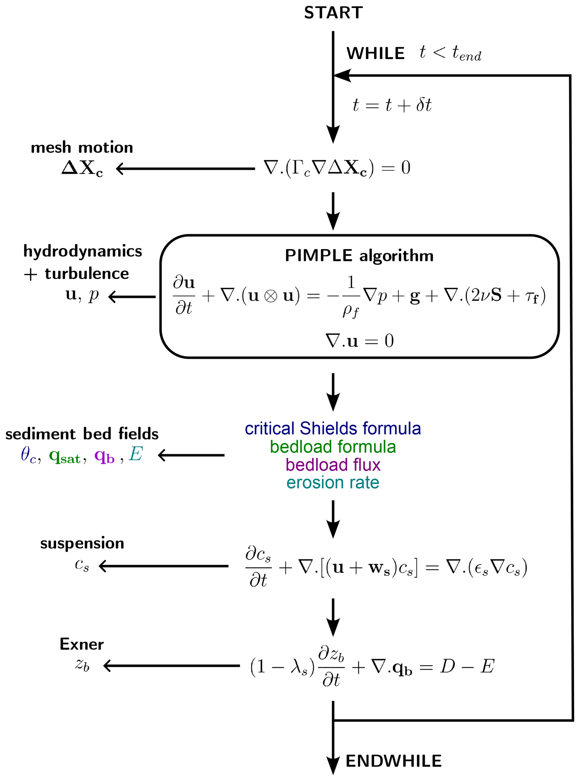
Figure 2 Flow chart of sedExnerFoam, illustrating the operations performed by the model during each time iteration.

The sequence of operations performed during a time iteration and their sequence are represented in Fig. 2. After solving the mesh deformation, the differential equations for the velocity field u, the pressure p (Eq. 1) as well as transport equations for fields related to turbulence modeling (Eqs. 4, 5) are first solved through the PIMPLE algorithm for transient solution which is detailed in Greenshields and Weller (2022). It consists of a mix of the SIMPLE (Semi-Implicit Method for Pressure-Linked Equations) from Patankar and Spalding (1983) and the PISO (Pressure Implicit with Splitting of Operators) from Issa (1986). An additional corrector loop called the PIMPLE loop is added above the PISO loop. During each time step, the velocity flux through the mesh faces is updated at every PIMPLE loop iteration, preserving the simulation stability at a higher Courant number (C_o>1). The PISO algorithm behavior is restored by disabling the PIMPLE loop. Once the hydrodynamics have been solved, the shear stress exerted on the bed is computed as well as the associated bedload and erosion flux. The transport equation for suspended sediment transport is solved, and the deposition flux is deduced from it. Lastly, the bed boundary motion is computed by explicitly solving the Exner equation. At the beginning of the next time iteration, the mesh is updated to match the new bed position.

3.2 Exner equation resolution

Let us integrate the Exner equation (Eq. 11) over the projection of a face f:

$$\begin{array}{}\text{(21)}& {\displaystyle \frac{\partial z_{\mathrm{b}}}{\partial t}}{|}_{\mathrm{f}}=-{\displaystyle \frac{\mathrm{1}}{S_{\mathrm{fp}}}}\sum _e({\mathit{q}}_{\mathrm{b},\mathrm{ep}}.{\mathit{n}}_{\mathrm{ep}})l_{\mathrm{ep}}+(D-E{)}_{\mathrm{f}},\end{array}$$

where $S_{\mathrm{fp}}=S_{\mathrm{f}}({\mathit{n}}_{\mathrm{f}}.{\mathit{e}}_{\mathrm{g}})$ is the projected area of face f with S_f face f area, and n_f is the face normal unit vector oriented outward of the computational domain. l_ep is the length of the projected edge, q_b,ep the projected bedload flux at edge e, and n_ep the projected normal edge vector, oriented outward with respect to face f. The users have the choice to use either an explicit Euler scheme or a second-order Adams-Bashforth scheme for temporal integration. The discretization scheme for the divergence flux term can be either centered (i.e. linear), upwind first order or upwind second order (i.e. linear upwind).

From Eq. (21), at each time step, an increment of bed elevation δz_b is computed for each face center. In OpenFOAM, the mesh geometry is defined by the vertices' coordinates. Thus, to impose a mesh motion, the vertical displacements computed at face centers need to be interpolated on the vertices. Particular caution must be given to the interpolation scheme to ensure mass conservation. A straightforward approach would be to linearly interpolate z_b from face centers to vertices. Although mass-conservative for 1D bathymetries on structured meshes, the method fails to preserve mass for 2D bathymetries on unstructured meshes. Jacobsen (2015) provided a detailed review of the various methods available for solving the Exner equation and analyzed their respective advantages and limitations. He proposed a mass-conservative interpolation scheme, which is the one implemented in the present model.

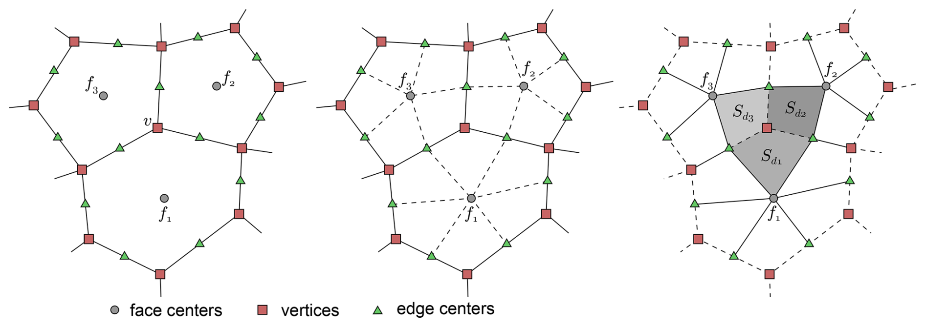
Figure 3 Construction of the dual mesh from the horizontal projection of the finite-area mesh. The dual mesh is formed by connecting the centers of the original mesh faces and the centers of their edges, illustrated here for three polygonal faces.

A dual mesh is constructed as depicted in Fig. 3. Each vertex v of the primary mesh serves as the center of a face in the dual mesh. The vertices defining this dual face consist of the neighboring primary faces f_i that share vertex v, as well as the centers of the edges for which v is an endpoint. The mass increment of the sediments contained under a face f is $m_{\mathrm{f}}={\mathit{\rho }}_{\mathrm{s}}{S}_{\mathrm{fp}}\mathit{\delta }{z}_{\mathrm{b}}{|}_{\mathrm{f}}$, where δz_b|_f is the face elevation increment. To ensure mass conservation during the interpolation process, the sum of the mass contained under every face must be the same when computing this sum for both the initial mesh and the dual mesh. The vertical displacement of each vertex δz_b|_v is then a linear combination of the displacements of the faces sharing this vertex. The weight associated with each face is proportional to the area of the quadrilateral defined by the face center, the vertex, and the centers of the two edges belonging to the face and sharing the vertex (see Fig. 3). Let us note the area of this quadrilateral S_df, the value of the elevation increment δz_b|_v associated to a vertex v is computed:

$$\begin{array}{}\text{(22)}& \mathit{\delta }{z}_{\mathrm{b}}{|}_{\mathrm{v}}={\displaystyle \frac{\mathrm{1}}{S_{\mathrm{v}}}}\sum _{\mathrm{f}}{S}_{\mathrm{df}}\mathit{\delta }{z}_{\mathrm{b}}{|}_{\mathrm{f}},\end{array}$$

where S_v is the area of the dual face whose center is the vertex v. It is equal to the sum of the area of each face associated quadrilateral: $S_{\mathrm{v}}={\sum }_{\mathrm{f}}{S}_{\mathrm{df}}$. Thus, the sum of the interpolation weights is equal to 1. This interpolation method is mass-conservative and also acts as a filter, as the bed increment is interpolated back and forth between the face centers, where the Exner equation is solved, and the vertices, where the mesh motion is imposed, which in turn updates the positions of the face centers. The final bed displacement at each face is computed in two steps: first, interpolation from faces to vertices, and then from vertices back to faces, with the face centers defined as the center of mass of the vertices composing each face. This filtering effect contributes to maintaining the numerical stability of the Exner equation solution.

3.3 Mesh motion

At each time step, solving the Exner equation gives a displacement for the bed boundary. For the finite volume mesh to adapt to the bed boundary motion and to preserve the mesh quality throughout the simulation, a mesh motion solver based on a Laplacian equation for cell center displacements is used:

$$\begin{array}{}\text{(23)}& \mathrm{\nabla }.\left({\mathrm{\Gamma }}_{\mathrm{c}}\mathrm{\nabla }\mathbf{\Delta }{X}_{\mathrm{c}}\right)=\mathrm{0},\end{array}$$

where Γ_c is the mesh diffusivity and ΔX_c is the displacement of the cell centers. Solving Eq. (23), new positions of the mesh cell centers are obtained. The mesh vertices' new coordinates are then interpolated from ΔX_c. The motion solver is defined in the file constant/dynamicMeshDict, and this study utilizes the displacementLaplacian solver.

Using a spatially non-uniform mesh diffusivity (Γ_c) makes it possible to prioritize mesh quality and control cell sizes in specific regions. Areas with lower Γ_c are more prone to mesh distortion, whereas regions with higher values help prevent excessive cell shrinking or expansion, provided that bed movement remains moderate. Several approaches are available for prescribing Γ_c, giving the user flexibility in defining its spatial distribution. As a general guideline, it is recommended to assign a high mesh diffusivity near the sediment bed interface to preserve mesh quality in this critical region. The following options, which can be selected in the configuration file constant/dynamicMeshDict, ensure this behavior:

• inverseDistance: ${\mathrm{\Gamma }}_{\mathrm{c}}=\mathrm{1}/l_{\mathrm{sb}}$

• quadratic inverseDistance: ${\mathrm{\Gamma }}_{\mathrm{c}}=\mathrm{1}/l_{\mathrm{sb}}^{\mathrm{2}}$

• exponential: ${\mathrm{\Gamma }}_{\mathrm{c}}=e^{-l_{\mathrm{sb}}}$

where l_sb is the distance to the sediment bed boundary.

One drawback of using the finite-volume method to compute mesh motion is the need to interpolate vertex displacements from the cell-centered displacements obtained from Eq. (23). This interpolation step can degrade mesh quality in regions where bed motion is highly non-uniform. In the worst-case scenario, severe distortion may cause some cells to collapse, ultimately leading to simulation failure. Among all the simulations conducted, one problematic case has been identified: the migration of a steep bedform. When the crest is sharp, the vertices located just above the crest, but not belonging to the bed boundary, may be displaced below the bed surface during the interpolation step. Reducing the aspect ratio of the near-bed cells has proven to be an effective way to mitigate this issue.

3.4 File structure of a case

The numerical setup is defined through a set of input files that specify the computational domain, physical parameters, boundary and initial conditions, and numerical options. Each file must be properly configured by the user before running the simulation. The following sections describe the purpose and required content of each file. The basic directory structure – i.e., all files required to run a sedExnerFoam simulation – is shown in Fig. 4. It is organized into three main folders, further explained below.

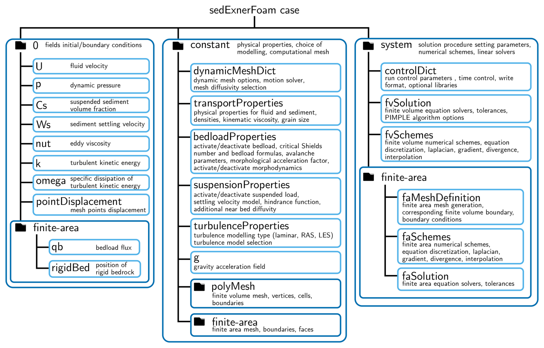
Figure 4 Case directory structure for a sedExnerFoam simulation, organized into three folders: 0 for initial conditions, constant for modeling options and physical properties, and system for time control and numerical settings.

3.4.1 Initial and boundary conditions

The initial time directory, usually named “0”, contains the initial conditions for all fields required by sedExnerFoam. Each field file defines both the initial field values and the boundary conditions applied to every patch of the mesh. The required fields include velocity (U), pressure (p), and, depending on the turbulence model employed, the relevant turbulent quantities. In Fig. 4, the setup illustrates the use of the k−ω SST turbulence model and consequently, the additional turbulent fields required are ν_t (nut), k (k), and ω (omega). The suspended sediment volume fraction (Cs) and settling velocity (Ws) must also be specified. The finite-area subdirectory contains the finite-area fields, including the bedload flux and, optionally, the position of a rigid bedrock. When a rigid bedrock is specified, the model restricts erosion to a predefined depth, ensuring that the non-erodible layer remains unaffected. This is achieved by iterating over all edges of the finite-area mesh and limiting the bedload flux whenever the sediment volume between the upwind face and the rigid bed is less than the flux through the edge. The initial time directory is read at the start of a simulation, providing the baseline from which the solution begins to evolve.

3.4.2 Constant directory

The constant directory contains the model configuration and physical properties, as well as the finite-volume and finite-area meshes stored in the polyMesh and finite-area subdirectories, respectively. The turbulence modeling approach (LES, RAS), and the specific model used is defined in the turbulenceProperties file. Additionally, the dynamicMeshDict file is used to select the mesh-motion solver and the mesh-diffusivity method to be applied. The fluid and sediment properties, such as densities, grain size, and fluid kinematic viscosity, are specified by the user in the transportProperties file. Modeling options related to sediment transport are separated into two files, suspensionProperties and bedloadProperties, each corresponding to one mode of sediment transport.

In suspensionProperties, the user can enable or disable suspended load, select both a formulation for the terminal settling velocity $w_{\mathrm{s}}^{\mathrm{0}}$ and a hindrance model from those summarized in Table 1, apply an additional wall diffusivity (see Eq. 20), and adjust the coefficients ${\mathit{ϵ}}_w^{\mathrm{0}}$ and ξ_w, as well as the limiter on the reference concentration $c_{\mathrm{b},\max }^{*}$ (see Eq. 18).

Stokes (1901)Fredsoe and Deigaard (1992)Soulsby (1997)Rubey (1933)Richardson and Zaki (1954)Camenen (2008)

Table 1 Available options in sedExnerFoam for computing the terminal settling velocity $w_{\mathrm{s}}^{\mathrm{0}}$ and hindrance functions F_h. Models are selected in suspensionProperties using the entries fallModel and hindranceModel.

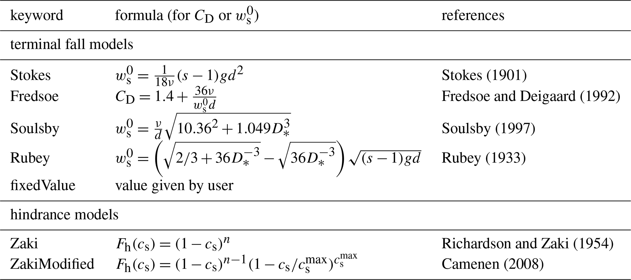
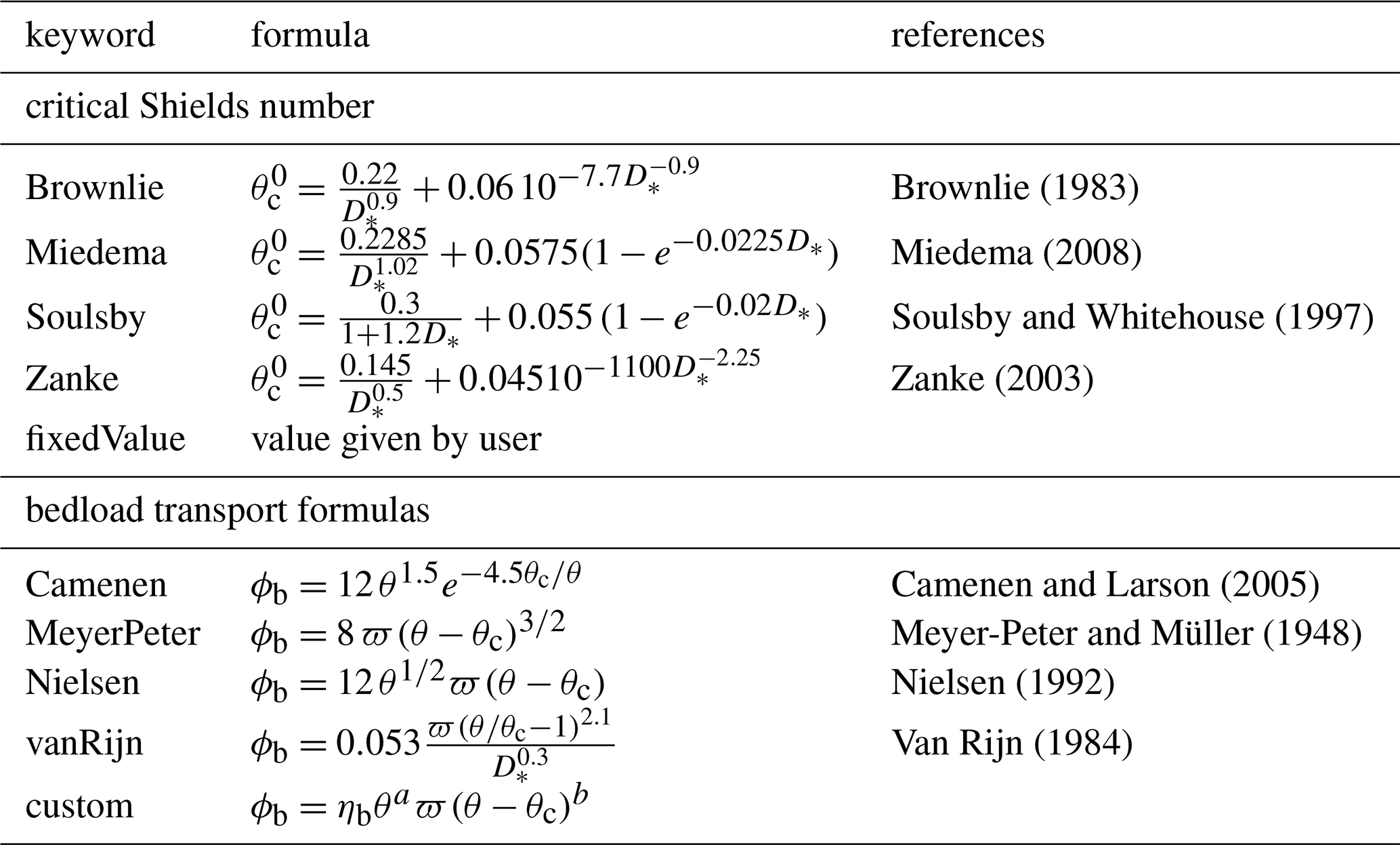
In bedloadProperties, the user can enable or disable bedload transport and morphological evolution, choose models for the critical Shields number and for the bedload formulation (see Table 2), activate the critical Shields number slope correction (Eq. 13), set the avalanche coefficient $q_{\mathrm{av}}^{\mathrm{0}}$, use a morphological acceleration factor that scales the bedload flux, and specify whether a rigid, non-erodible bed exists beneath the sediment layer, which limits the maximum erosion depth.

Brownlie (1983)Miedema (2008)Soulsby and Whitehouse (1997)Zanke (2003)Camenen and Larson (2005)Meyer-Peter and Müller (1948)Nielsen (1992)Van Rijn (1984)

Table 2 Available formulas in sedExnerFoam to compute the critical Shields number on a flat bed ${\mathit{\theta }}_{\mathrm{c}}^{\mathrm{0}}$ from fluid and sediment properties, and the dimensionless bedload flux ϕ_b from the Shields number θ. Models are selected in bedloadProperties using the entries criticalShieldsModel and bedloadModel.

3.4.3 Case run control

The system directory in OpenFOAM contains files that control how simulations are executed. Among them, the controlDict file specifies the simulation time controls, including start and end times, time-step settings, and also defines optional libraries and post-processing utilities to be executed during the simulation. The fvSchemes file, which specifies the numerical discretization schemes, and the fvSolution file, which sets the linear solvers and algorithmic controls. Depending on the case setup, additional configuration files may appear in this directory. The finite-area subdirectory contains all files related to the finite-area method, including the finite-area mesh definition in faMeshDefinition and the numerical schemes and linear solvers in faSchemes and faSolution, respectively. Together, these files govern the computational parameters, numerical methods and overall runtime behavior of the simulation.

4 Model validation

A series of tests is presented both to illustrate the model behavior of sedExnerFoam and to validate it against either analytical solutions or experimental results. The tests are chosen to isolate one physical process at a time. They are organized as follows: two tests involving suspended load transport only are first presented (1D and 2D). Next, the case of an idealized dune migration problem (1D) for which an analytical solution exists is investigated. At last, the conservation of mass is illustrated by means of two tests on suspended sediment deposition and avalanches (1D and 2D). Most of these tests are part of a continuous integration process available on the GitHub repository.

4.1 Suspension under equilibrium condition

A classical test is the suspension of sediment in a straight flume under equilibrium conditions, which has been extensively studied (van Rijn, 1984; Lyn, 1988; Muste et al., 2005). A fully developed flow in a channel is considered. The channel is supposed to be long enough so that the vertical profiles of velocity and turbulent eddy viscosity are stationary. Under equilibrium conditions, the vertical profile of suspended sediment concentration is the result of a balance between the gravity, which makes the particles settle at a velocity w_s, and the mixing induced by turbulence. Let w_s denote the magnitude of w_s, the transport equation for the suspended load (Eq.  7) reduces to:

$$\begin{array}{}\text{(24)}& {\displaystyle \frac{\mathrm{d}}{\mathrm{d}z}}\left(w_{\mathrm{s}}{c}_{\mathrm{s}}+{\mathit{ϵ}}_{\mathrm{s}}{\displaystyle \frac{\mathrm{d}{c}_{\mathrm{s}}}{\mathrm{d}z}}\right)=\mathrm{0}.\end{array}$$

Depending on the shear stress exerted on the bed, granular material is eroded and suspended in the water column. Then, the turbulent diffusion uplifts the particles until an equilibrium is reached. Assuming a parabolic turbulent viscosity profile, ${\mathit{\nu }}_{\mathrm{t}}\left(z\right)=u_{*}\mathit{\kappa }z(H-z)$, where κ=0.41 is the von Kármán constant, the solution of Eq. (24) between the reference level $\mathit{\delta }{z}_{\mathrm{b}}^{*}$, where the concentration is the reference concentration $c_{\mathrm{b}}^{*}$, and the top of the water column H is the so-called Rouse profile:

$$\begin{array}{}\text{(25)}& c_{\mathrm{s}}\left(z\right)=c_{\mathrm{b}}^{*}({\displaystyle \frac{H-z}{z}}{\displaystyle \frac{\mathit{\delta }{z}_{\mathrm{b}}^{*}}{H-\mathit{\delta }{z}_{\mathrm{b}}^{*}}}{)}^{R_o},\end{array}$$

where $R_o={\mathit{\sigma }}_{\mathrm{c}}{w}_{\mathrm{s}}/\mathit{\kappa }{u}_{*}$ is the Rouse number.

To validate the suspended load component of the model, numerical results are compared with experimental data from Lyn (1988). The experiment was conducted in a 13 m-long and 26.7 cm-wide flume with a bottom covered by a layer of sand. Flow and suspended sediments concentration measurements were made approximately 9 m downstream of the channel entrance. The experiment parameters are summarized in Table 3.

Table 3 Parameters of four tests from Lyn (1988) experiment. Particles diameter d, settling velocity w_s, mean water velocity $\stackrel{\mathrm{‾}}{u}$, water depth, friction velocity u_* and Rouse number R_o.

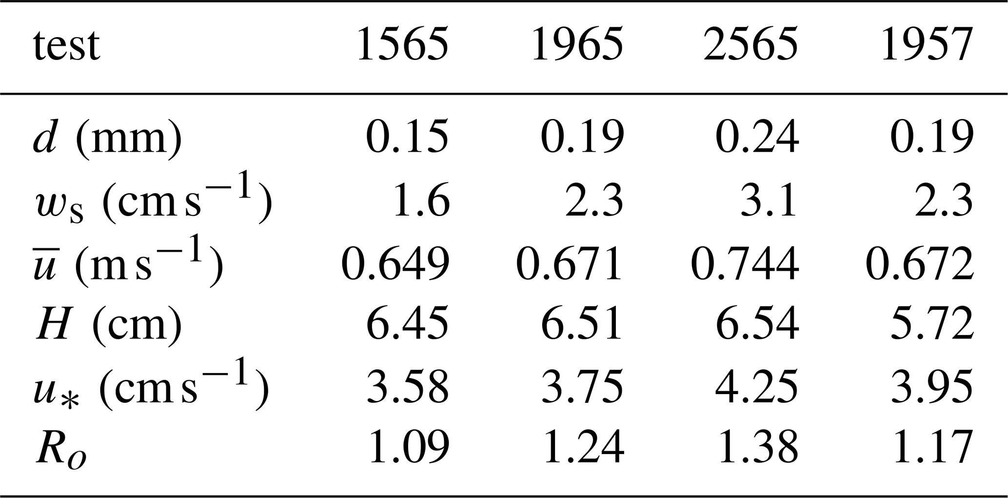
For the four tests, measurements of the velocity field, the velocity correlation, and the suspended sediment concentration profiles are available.

The four equilibrium bed experiments are reproduced numerically. A 1D mesh is employed, consisting of a column of 120 cells oriented along the vertical z-direction. Cyclic boundary conditions are applied in the stream-wise x-direction, and the mesh is refined near the bed. Only the x-component u of the velocity field is non-zero. For all four simulations, the k−ω SST turbulence model is employed, and the mesh resolution near the bed is maintained at $z^{+}\approx \mathrm{1}$ to ensure adequate resolution and an accurate estimation of the bed shear stress. Here, $z^{+}=u_{*}{z}_{\mathrm{1}}/\mathit{\nu }$ denotes the distance of the first cell center from the bed boundary in wall units, where z₁ is the distance to the sediment bed boundary.

The free surface is not considered, and a rigid lid is applied at the top, with zero gradient condition for the turbulent kinetic energy k, a Dirichlet condition for ω, and a slip boundary condition for the velocity u. To take into account the bed roughness effect on the hydrodynamics, the boundary condition for ω proposed by Wilcox (1998) is used:

$$\begin{array}{}\text{(26)}& \mathit{\omega }={\displaystyle \frac{u_{*}^{\mathrm{2}}}{\mathit{\nu }}}{S}_{\mathrm{R}},\end{array}$$

where S_R is defined as a function of the roughness Reynolds number $k_{\mathrm{s}}^{+}=u_{*}{k}_{\mathrm{s}}/\mathit{\nu }$ as follows:

$$\begin{array}{}\text{(27)}& {\displaystyle }& {\displaystyle }{S}_{\mathrm{R}}={\left({\displaystyle \frac{\mathrm{200}}{k_{\mathrm{s}}^{+}}}\right)}^{\mathrm{2}}& {\displaystyle }\text{for }{k}_{\mathrm{s}}^{+}\le \mathrm{5},\text{(28)}& {\displaystyle }& {\displaystyle }{S}_{\mathrm{R}}={\displaystyle \frac{\mathrm{100}}{k_{\mathrm{s}}^{+}}}+\left[\left({\displaystyle \frac{\mathrm{200}}{k_{\mathrm{s}}^{+}}}\right)-{\displaystyle \frac{\mathrm{100}}{k_{\mathrm{s}}^{+}}}\right]e^{\mathrm{5}-k_{\mathrm{s}}^{+}}& {\displaystyle }\text{for }{k}_{\mathrm{s}}^{+}>\mathrm{5}.\end{array}$$

The transient problem is solved, and the simulations are run until a steady state has been reached, taking a few seconds on a single CPU core. The numerical results are plotted alongside the experimental data from Lyn (1988) in Fig. 5.

Figure 5 Velocity and suspended sediment concentration profiles from numerical simulations and comparison with experimental data from Lyn (1988).

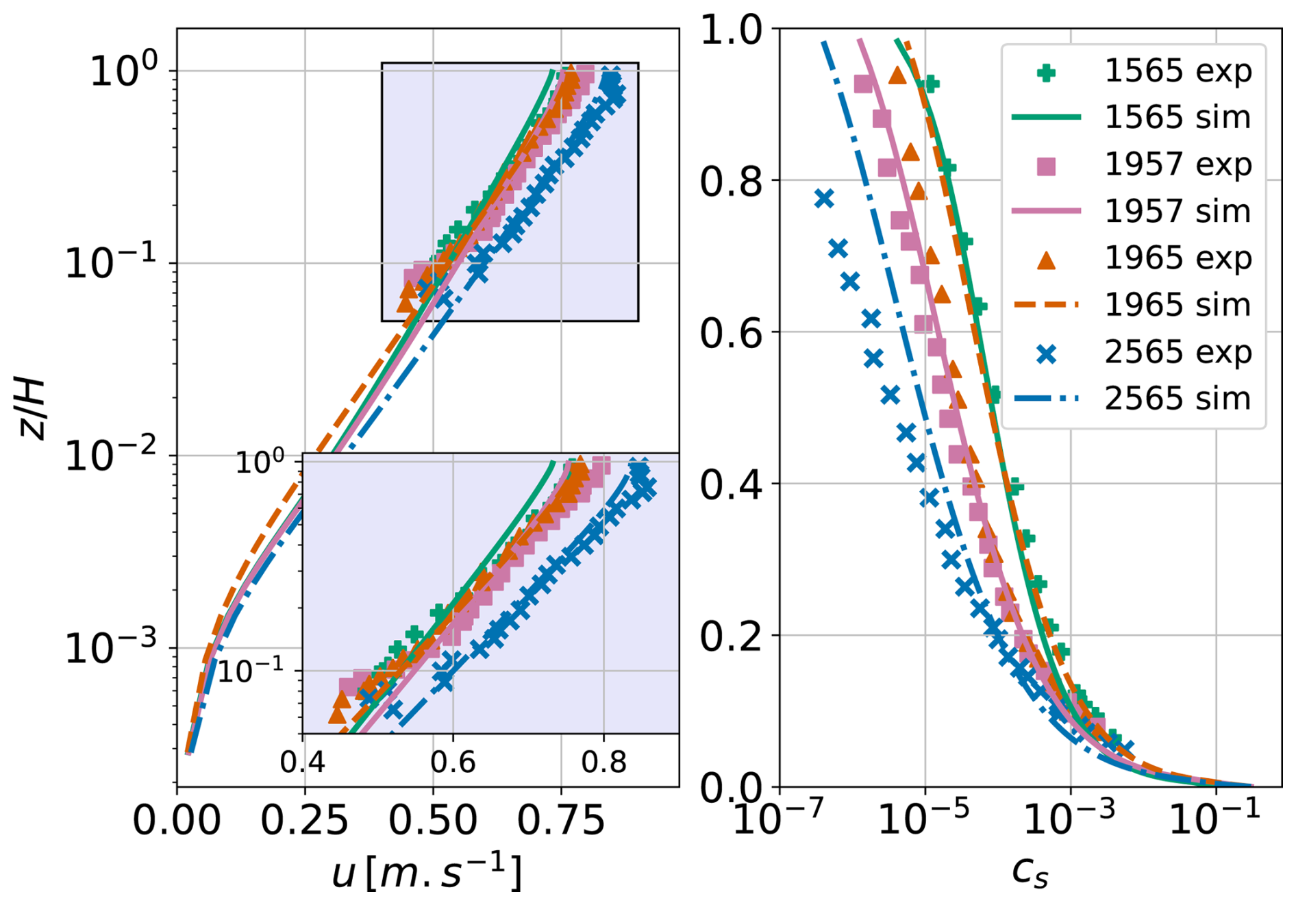
Overall, the numerical results show good agreement with the experimental data. For the suspended sediment profiles, it is observed that in cases 2565 and 1957, the suspended sediment concentration is slightly overestimated, particularly in the upper part of the water column. To quantitatively assess the agreement between the numerical and experimental profiles, the symmetric mean absolute percentage error (SMAPE) of the logarithm of the sediment volume fraction is computed as follows:

$$\begin{array}{}\text{(29)}& \text{SMAPE}={\displaystyle \frac{\mathrm{2}}{N}}\sum {\displaystyle \frac{\left|{\log }_{\mathrm{10}}\right(c_{\mathrm{s}}^{\text{num}})-{\log }_{\mathrm{10}}(c_{\mathrm{s}}^{\text{exp}}\left)\right|}{\left|{\log }_{\mathrm{10}}\right(c_{\mathrm{s}}^{\text{num}}\left)\right|+\left|{\log }_{\mathrm{10}}\right(c_{\mathrm{s}}^{\text{exp}}\left)\right|}},\end{array}$$

where N is the number of measurements available in the experimental test considered, $c_{\mathrm{s}}^{\text{exp}}$ is the experimental sediment volume fraction, and $c_{\mathrm{s}}^{\text{num}}$ is the sediment volume fraction obtained from the numerical simulation and linearly interpolated to the elevations corresponding to the experimental data. The resulting errors are 4.34 % for case 1565, 8.29 % for case 1965, 6.64 % for case 2565, and 2.46 % for case 1957. These results were obtained without any calibration of the model coefficients, and an improved fit could likely be achieved by adjusting parameters such as the turbulent Schmidt number σ_c, the near-bed diffusivity coefficients ${\mathit{ϵ}}_w^{\mathrm{0}}$ and ξ_w (Eq. 20), or the equivalent sand roughness height k_s.

4.2 Suspension development

Another test for the suspended load is the development of suspension in a channel, when the flow encounters an abrupt transition from a non-erodible bed to an erodible bed. Initially, the flow is clear, and it becomes loaded with sediments until an equilibrium is reached. For this problem, the results are compared with a pseudo-analytical solution derived by Hjelmfelt and Lenau (1970). In order to obtain this solution, some assumptions are made.

1. The sediment is uniformly advected at the mean flow velocity $\stackrel{\mathrm{‾}}{u}$.

2. The turbulent viscosity vertical profile is assumed parabolic, ${\mathit{\nu }}_{\mathrm{t}}=\mathit{\kappa }{u}_{*}z(\mathrm{1}-z/H)$ for $z\in [\mathit{\delta }{z}_{\mathrm{b}}^{*},H]$ where $\mathit{\delta }{z}_{\mathrm{b}}^{*}$ is the reference level and H, the water depth.

3. The concentration at $z=\mathit{\delta }{z}_{\mathrm{b}}^{*}$ is supposed to be constant along the flume and equal to $c_{\mathrm{b}}^{*}$, the reference concentration.

4. The horizontal turbulent diffusion is neglected.

Based on those assumptions, Hjelmfelt and Lenau (1970) simplified the transport equation for the suspended load and derived an analytical solution. They performed a separation of variables and used the Sturm-Liouville theory to obtain a solution, which only depends on the Rouse number. A first numerical simulation is performed for which all assumptions apart from the fourth one are respected. A water depth of H=0.1 m is considered, the mean velocity is $\stackrel{\mathrm{‾}}{u}=\mathrm{0.9}\mathrm{m}{\mathrm{s}}^{-\mathrm{1}}$, and the Rouse number is equal to 0.5, which corresponds to a regime in which suspended load is the dominant sediment transport mode. The results are presented in Fig. 6.

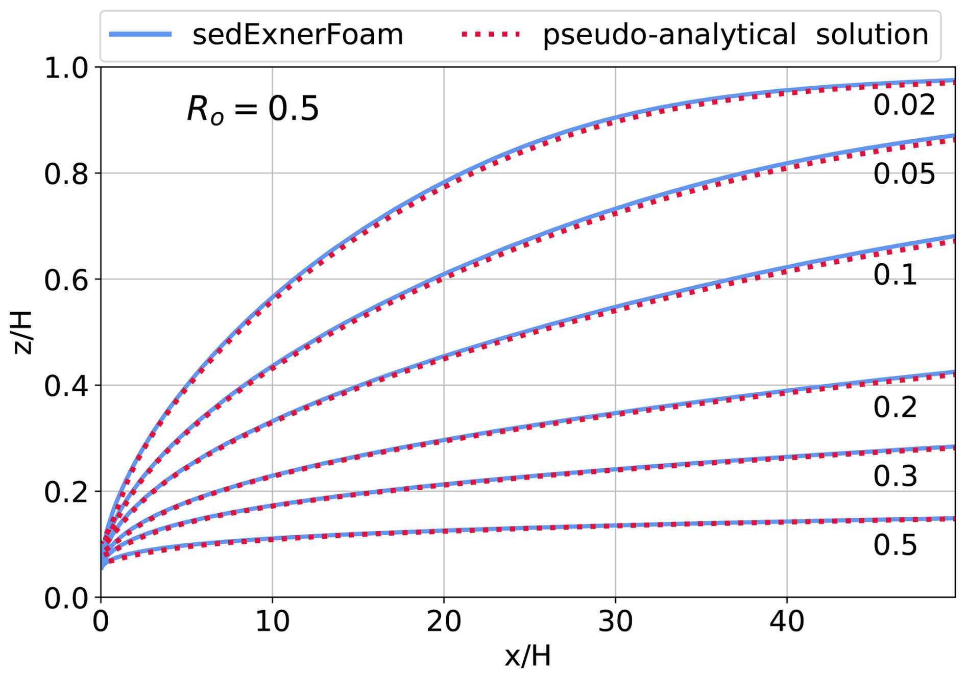
Figure 6 Isolines of $c_{\mathrm{s}}/c_{\mathrm{b}}^{*}$ for a Rouse number of 0.5 with assumptions from Hjelmfelt and Lenau (1970) enforced except the null horizontal turbulent diffusion. Solid blue curves represent the model results and the dotted red ones the pseudo-analytical solution.

In this case, the numerical and pseudo-analytical solutions are almost identical, suggesting that the stream-wise turbulent diffusivity (assumption 4) is indeed negligible. However, some of the assumptions from Hjelmfelt and Lenau (1970) are normally not verified. The vertical velocity profile is not uniform, the concentration at the reference level may vary in space and reach an equilibrium after some distance from the inlet, and lastly, the turbulent eddy-viscosity profile is not exactly parabolic.

The particle diameter was set to d=0.12 mm, corresponding to a settling velocity of $w_{\mathrm{s}}=\mathrm{0.773}\mathrm{cm}{\mathrm{s}}^{-\mathrm{1}}$ and a Rouse number of R_o=0.5. Although tests were conducted with different Rouse numbers, only the case R_o=0.5 is presented in this work. The same mean flow velocity $\stackrel{\mathrm{‾}}{u}=\mathrm{0.9}\mathrm{m}{\mathrm{s}}^{-\mathrm{1}}$ is taken, and the resulting shear stress exerted on the bed corresponds to the bed friction velocity $u_{*}=\mathrm{3.77}\mathrm{cm}{\mathrm{s}}^{-\mathrm{1}}$. The k−ω SST turbulence model and the rough wall boundary from Wilcox (1998) (Eq. 26) condition is used for ω with a roughness height k_s=2.5 d.

A first 1D simulation is performed without sediment to obtain vertical profiles for u, k, and ω corresponding to a fully developed channel flow. The fields u, k and ω are extracted from this first simulation and used as the inlet boundary condition for the second simulation, for which suspension is activated. The flow entering the domain being already fully developed, only c_s varies with the x-position. The mesh consists of a 2D structured mesh, more refined close to the bed to ensure the condition $z^{+}\approx \mathrm{1}$ (n_x=2000, n_z=100). The results are extracted after 50 s of simulation, requiring 10 h of wall-clock time on 5 CPU cores. Isolines of $c_{\mathrm{s}}/c_{\mathrm{b}}^{*}$ values from the model and the pseudo-analytical solution are presented in Fig. 7. To compute the pseudo-analytical solution, the reference level was chosen equal to $\mathit{\delta }{z}_{\mathrm{b}}^{*}=\mathrm{0.05}H$ as in the work of Hjelmfelt and Lenau (1970), and the reference concentration is taken equal to $c_{\mathrm{b}}^{*}=\mathrm{0.025}$ and applied as a boundary condition at the elevation $z=\mathit{\delta }{z}_{\mathrm{b}}^{*}$.

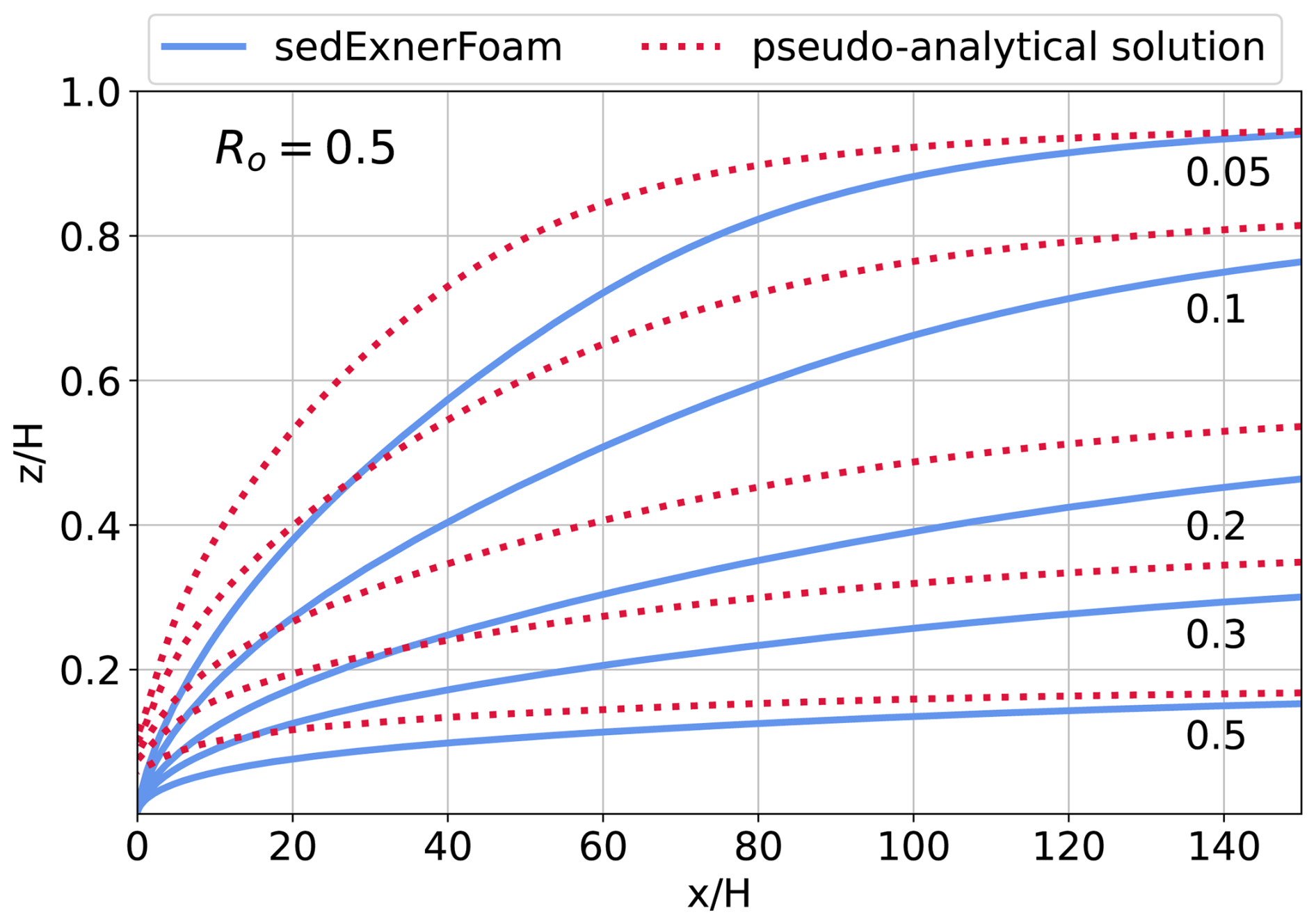
Figure 7 Isolines of $c_{\mathrm{s}}/c_{\mathrm{b}}^{*}$. Comparison between pseudo-analytical solution from Hjelmfelt and Lenau (1970) (red dotted lines) and the model solution (solid blue lines) without enforcement of the assumptions used to derive the pseudo-analytical solution.

Compared with the situation where the assumptions on the flow is enforced (see Fig. 6), the model results do not match the pseudo-analytical solution, but the global behavior remains the same. Starting from no suspension, the suspended sediment quantity gradually increases with the distance to the inlet until reaching an equilibrium situation where the settling and the turbulent diffusion cancel each other out. Figure 8 shows the vertical suspended sediment volume fraction c_s profiles at different positions along the channel and shows the convergence toward an equilibrium solution close to a Rouse profile.

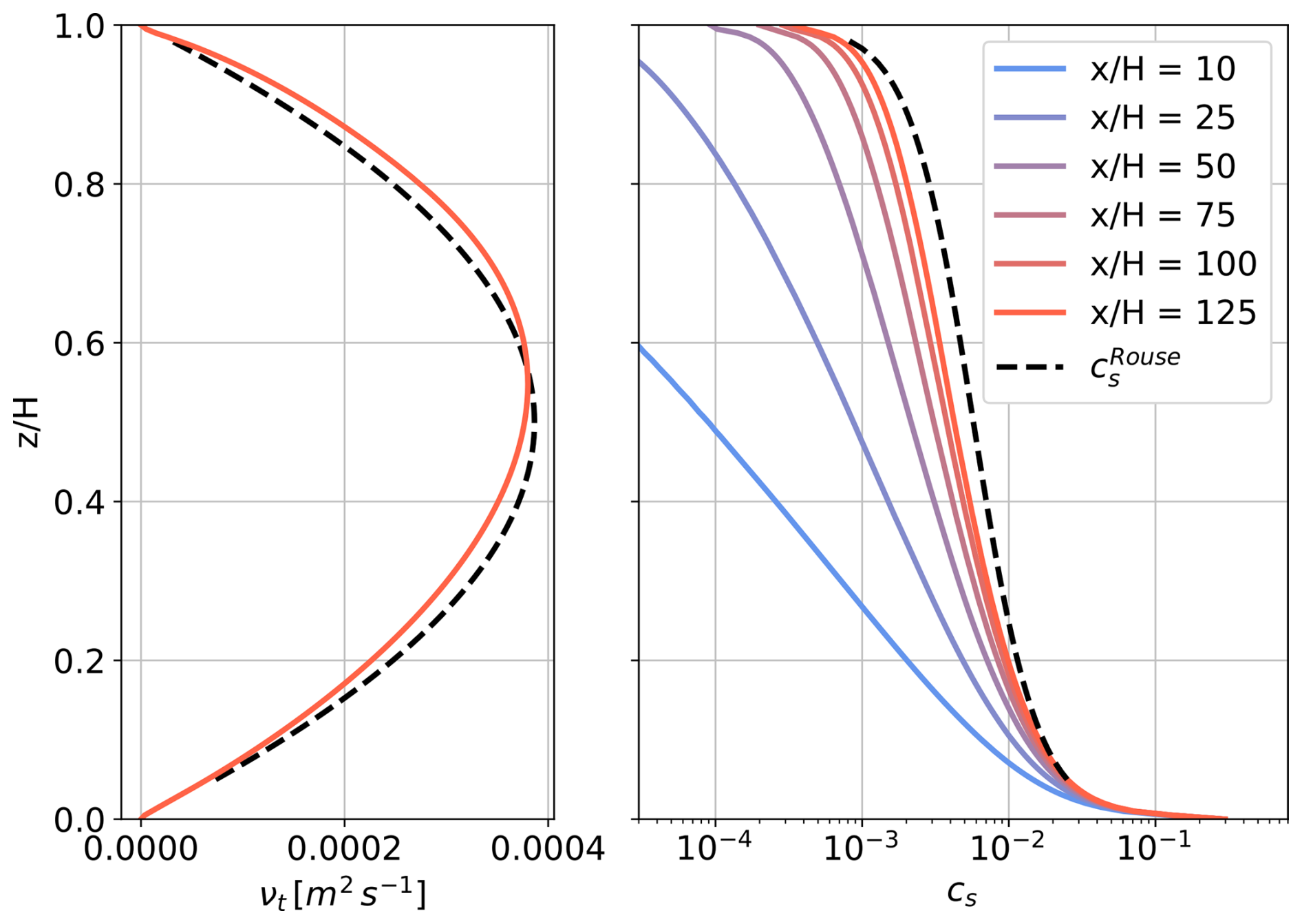
Figure 8 On the left-hand side, the turbulent eddy viscosity obtained with the model (solid line) and the theoretical parabolic profile (black dashed line). On the right-hand side, vertical profiles of c_s at different x-positions in the channel. For comparison, the Rouse profile corresponding to the pseudo-analytical solution in Fig. 7 is also plotted (black dashed line).

As stated previously, the discrepancies with the pseudo-analytical solution arise from the unrealistic assumptions made in its derivation. These include the assumption that suspended sediments are advected by the mean flow, the use of a parabolic eddy viscosity profile, and the assumption of local equilibrium at the reference level. A better agreement could yet be found, for instance, by adjusting the boundary conditions for ω at the top and bottom boundaries, which would affect the shape of ν_t profile. Another calibration parameter is the reference concentration at the reference level, which is the bottom boundary condition of the pseudo-analytical solution.

4.3 Idealized dune migration

As a first benchmark for the Exner equation (Eq. 11), an idealized 1D dune migration model for which an analytical solution exists is presented. In this case, a highly simplified flow is considered in order to focus on the behavior of the Exner equation without the added complexity of the hydrodynamics (see Fig. 9). The fluid is topped by a rigid lid placed at an elevation H from the bottom. The flow is assumed vertically uniform with a constant discharge per unit width Q. The depth-averaged velocity is obtained by conservation of mass, $U=Q/(H-z_{\mathrm{b}})$.

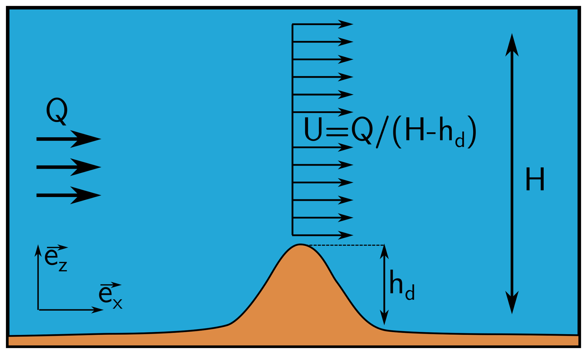
Figure 9 Schematic of the idealized dune migration case showing the main parameters and illustrating the relationship between bed elevation and depth-averaged velocity.

In this simplified case, only bedload transport is considered. To be able to derive an analytical solution of the Exner equation, the bedload q_b must be expressed as a function of the bed elevation z_b. This is done by assuming that the bedload is a power law of the depth-averaged velocity U, $q_{\mathrm{b}}={\mathit{\alpha }}_{\mathrm{d}}{U}^{{\mathit{\beta }}_{\mathrm{d}}}$, where α_d and β_d are two positive constants. The Exner equation (Eq. 11) simplifies to:

$$\begin{array}{}\text{(30)}& {\displaystyle }& {\displaystyle \frac{\partial z_{\mathrm{b}}}{\partial t}}+c\left(z_{\mathrm{b}}\right){\displaystyle \frac{\partial z_{\mathrm{b}}}{\partial x}}=\mathrm{0},\text{(31)}& {\displaystyle }& {\displaystyle }c\left(z_{\mathrm{b}}\right)={\displaystyle \frac{\partial q_{\mathrm{b}}}{\partial z_{\mathrm{b}}}}={\displaystyle \frac{{\mathit{\alpha }}_{\mathrm{d}}{\mathit{\beta }}_{\mathrm{d}}{Q}^{{\mathit{\beta }}_{\mathrm{d}}}}{(H-z_{\mathrm{b}}{)}^{{\mathit{\beta }}_{\mathrm{d}}+\mathrm{1}}}},\end{array}$$

where c(z_b), is the celerity of the bedform. Starting with a given initial bedform $z_{\mathrm{b}}(x,t=\mathrm{0})=F_{\mathrm{0}}\left(x\right)$, the solution to Eq. (30) is obtained with the method of characteristics (McOwen, 1996) leading to $z_{\mathrm{b}}(x,t)=F_{\mathrm{0}}(x-ct)$. Depending on F₀, shocks may develop as the bedform migrates. A shock occurs if, over at least one interval ℐ∈ℝ, the function $G:x\to c\left(F_{\mathrm{0}}\right(x\left)\right)$ is decreasing. The dune celerity c being an increasing function of z_b, shocks will arise if the initial bedform F₀ exhibits at least one negative slope. In this idealized dune migration case, the initial dune profile is Gaussian:

$$\begin{array}{}\text{(32)}& F_{\mathrm{0}}(x,t)=h_{\mathrm{d}}{e}^{-{\left({\displaystyle \frac{x-x_{\mathrm{d}}^{\mathrm{0}}}{{\mathit{\sigma }}_{\mathrm{d}}}}\right)}^{\mathrm{2}}},\end{array}$$

with h_d the height of the dune, $x_{\mathrm{d}}^{\mathrm{0}}$ the initial position of the dune's crest and σ_d a parameter linked to the dune width such that $F_{\mathrm{0}}(x_{\mathrm{d}}\pm \sqrt{\ln \left(\mathrm{2}\right)}{\mathit{\sigma }}_{\mathrm{d}})=\mathrm{0.5}{h}_{\mathrm{d}}$.

With this initial dune profile, a shock wave will form where the bed slope becomes vertical on the lee side of the dune. To know the position and time of the shock, it is necessary to find the position $x_{\mathrm{0}}^{*}$ defined as follows: $G^{\prime }\left(x_{\mathrm{0}}^{*}\right)={min}_{x\in \mathcal{R}}\left(G\left(x\right)\right)$. It corresponds to the initial position of the point belonging to the characteristic line on which the first shock occurs. The breaking time is then obtained as $t^{*}=-\mathrm{1}/G^{\prime }\left(x_{\mathrm{0}}^{*}\right)$ and the shock position x^* as well by advection of $x_{\mathrm{0}}^{*}$ along its characteristic line, $x^{*}=x_{\mathrm{0}}^{*}+G\left(x_{\mathrm{0}}^{*}\right)t^{*}$.

The following parameters are chosen:

• flow properties, H=1 m and $Q=\mathrm{1}{\mathrm{m}}^{\mathrm{2}}{\mathrm{s}}^{-\mathrm{1}}$

• bedload flux, α_d=0.05 and β_d=1.5

• dune properties, h_d=0.1 m, σ_d=0.6 m

For this configuration, the breaking time is $t^{*}=\mathrm{24.67}\mathrm{s}$ and the shock position $x^{*}=\mathrm{4.51}\mathrm{m}$. A solution to Eq. (30) is sought for the time interval between t=0 and the breaking time t^*. A second-order Adams-Bashforth scheme is used for time integration and a linear-upwind scheme for the advective term discretization. A comparison between the model results and the analytical solution is presented in Fig. 10.

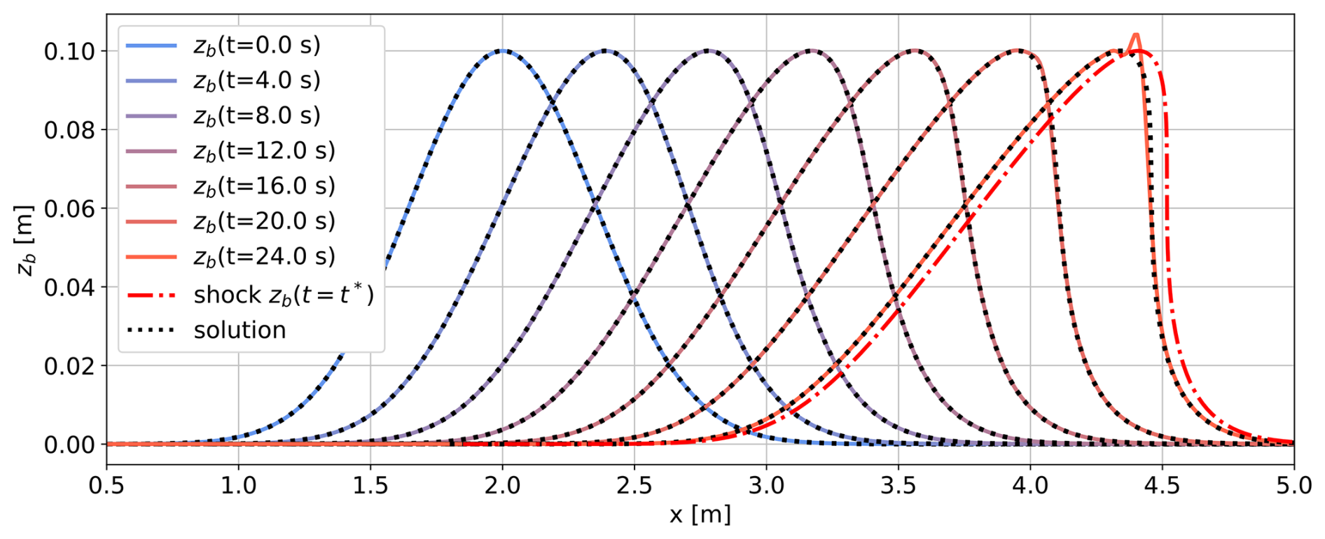
Figure 10 Bed level evolution of an initially Gaussian dune during an idealized transport scenario, comparing model results (solid lines) with the analytical solution (black dotted lines).

Overall, the model fits well with the analytical solution except when the time gets close to the breaking time, where a small instability starts to develop at the dune's crest. Figure 11 illustrates how the chosen numerical schemes affect the solution stability and precision.

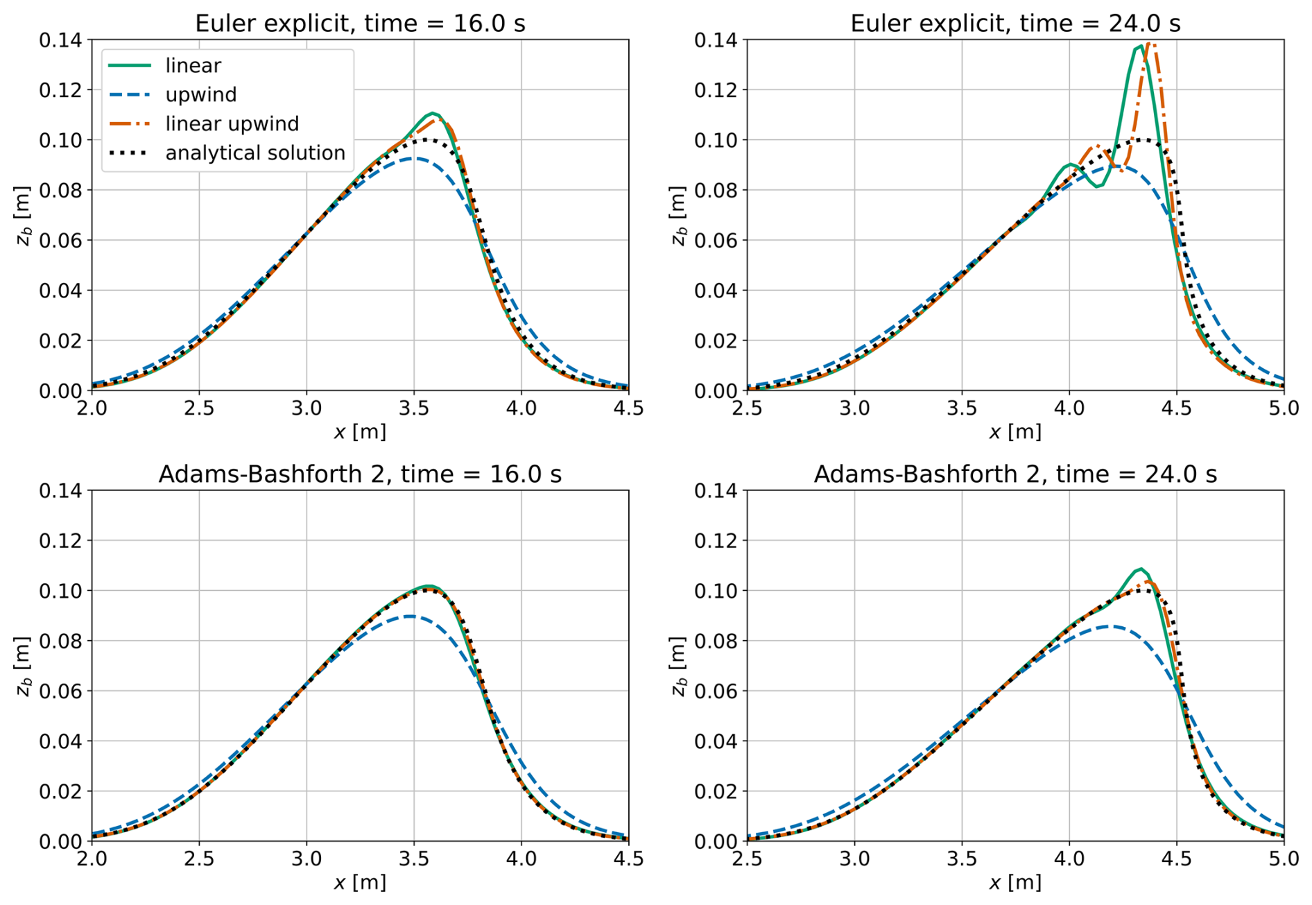
Figure 11 Comparison of bed levels in an idealized dune migration obtained from numerical simulations using three different advective schemes and two temporal integration schemes (Euler explicit top, Adams-Bashforth 2 bottom) with the analytical solution at intermediate (left) and near-breaking (right) times.

At the dune front, the gradient of z_b becomes significant, and, consequently, the gradient of z_b also increases. Depending on the numerical schemes used, this can trigger oscillations. Using the Euler explicit scheme for time integration, the use of a second-order scheme for advection leads to instabilities appearing on the crest of the dune. On the other hand, the low-order upwind scheme introduces numerical diffusion, resulting in reduced predictive accuracy, but ensures numerical stability. A better match between the numerical results and the analytical solution is achieved using a second-order scheme for the temporal term (Adams-Bashforth 2) as the numerical solution no longer oscillates.

As stated in Sect. 3.2, the interpolation from faces to vertices needed to enforce mesh motion acts as a filter. However, depending on the case, it may not be sufficient to suppress the appearance of numerical instabilities, in particular in regions presenting steep slopes. The use of an avalanche model (Eq. 15) brings more stability by limiting the maximum bed slopes. However, it is not used in this example as no analytical solution can be derived for this problem if the avalanche mechanism is taken into account.

From the results presented in Fig. 11, the combination of a second-order Adams-Bashforth scheme for the time integration and a linear or linear-upwind scheme for the bedload flux discretization, both being second-order schemes, seems to offer the best compromise between stability and accuracy. Choosing an Euler explicit time scheme tends to trigger instabilities, while the use of an order 1 upwind scheme leads to more stability at the cost of accuracy. To further illustrate the different behaviors of the possible scheme combinations and for different mesh refinements, multiple simulations are performed by varying the grid size and the numerical schemes, and the results are compared with the analytical solution.

The stability of the numerical solution is related to the mesh refinement through the maximum Courant number, whose evaluation is straightforward as the celerity of bedforms c is known (Eq. 30). The maximum Courant number is then $max\left(C_o\right)=c(z_{\mathrm{b}}=h_{\mathrm{d}})\mathit{\delta }t/\mathit{\delta }x$ where δt is the time step value and δx the width of the mesh faces in the x-direction, the mesh being uniform. The accuracy of the numerical solution is evaluated using the Root Mean Square Error (RMSE):

$$\begin{array}{}\text{(33)}& \text{RMSE}=\sqrt{{\displaystyle \frac{\mathrm{1}}{N_{\mathrm{F}}}}\sum _{\mathrm{f}}(z_{\mathrm{b}}^n{|}_{\mathrm{f}}-z_{\mathrm{b}}^s{|}_{\mathrm{f}}{)}^{\mathrm{2}}},\end{array}$$

where the index f stands for the finite area mesh faces, N_F the number of faces of the mesh, $z_{\mathrm{b}}^n{|}_{\mathrm{f}}$ is the elevation of face f center (numerical solution) and $z_{\mathrm{b}}^s{|}_{\mathrm{f}}$ is the analytical bed elevation at face f center. Each simulation is represented by a point in Fig. 12.

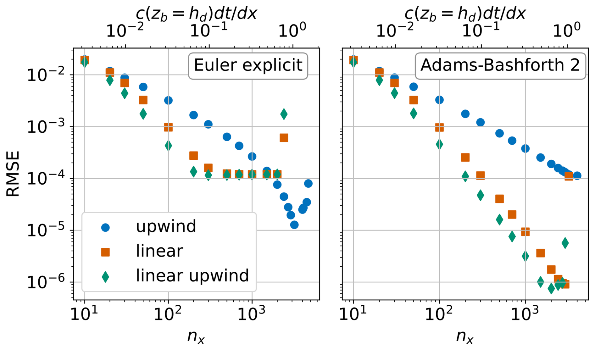
Figure 12 Root mean square error for different combinations of numerical schemes and mesh refinements. The time step is constant (δt=0.05 s) for all simulations, with only the number of faces (n_x) in the finite area mesh varying. The maximum Courant number, based on the bedform celerity, is indicated on the top axis.

The simulations were performed using a constant time step. For low Courant numbers, associated with poor mesh quality, all simulations remain stable and exhibit similar errors. As the mesh quality increases, the RMSE decreases but at a faster rate for second-order schemes for bedload advection until the solution becomes unstable when the maximum Courant number gets close to 1. The sudden rise of RMSE values for high mesh resolution is a sign of those instabilities. The use of an upwind scheme allows for the use of a higher Courant number without the simulation failing. This is due to the numerical diffusion that this first-order scheme involves. When using an Euler explicit time scheme along with one of the second-order schemes for advection, it is observed that the RMSE no longer depends on the mesh resolution for values of maximum Courant number of 0.1 and higher until the appearance of instabilities. It shall be recalled here that a filtering process is applied on the numerical solution at each time step as the bed elevation increment is interpolated from faces to vertices (discussed in Sect. 3.2). The results presented support the use of a combination of a second-order Adams-Bashforth scheme along with a linear or linear-upwind scheme to ensure both stability and accuracy.

These simulations complete in a few seconds on a single CPU core.

4.4 Sediment settling

A still basin of depth H=1 m is initially uniformly loaded with a volume fraction $c_{\mathrm{s}}^{\mathrm{0}}=\mathrm{0.05}$ of suspended sediment corresponding to a mass concentration of 132 kg m⁻³. As the suspended sediment deposit, the bed level rises up and reaches a final elevation $z_{\mathrm{bed}}=\frac{c_{\mathrm{s}}^{\mathrm{0}}}{\mathrm{1}-{\mathit{\lambda }}_{\mathrm{s}}}H$, where λ_s is the porosity of the deposited granular material. The settling velocity being set to $w_{\mathrm{s}}=\mathrm{3.59}\mathrm{cm}{\mathrm{s}}^{-\mathrm{1}}$, the time at which the last sediment deposit on the bed is $t=\frac{H-z_{\mathrm{bed}}}{w_{\mathrm{s}}}$. The variation over time of the sediment mass distribution between suspension and deposited sediments is represented in Fig. 13.

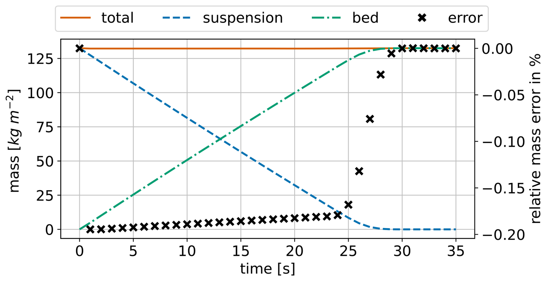
Figure 13 Time evolution of sediment mass per unit area, divided into suspended and deposited fractions, during deposition in a still basin. Relative error (%) of the total mass is shown by black crosses.

During each time iteration, the equation for the concentration of suspended sediments is solved, and the erosion/deposition flux is computed, resulting in an updated sediment bed elevation via the Exner equation (see Fig. 2). Since the mesh motion is resolved at the beginning of the time iteration, the bed level increment computed at a given step only affects the mesh geometry in the subsequent time step. Consequently, there is a one-time-step delay in the morphological response of the bed, which introduces a temporary error in the total sediment mass. However, this error vanishes once all suspended sediments have settled.

Another settling case is presented, this time a 2D case with non-uniform settling. The computational domain is conic-shaped, wider at the bottom (5 cm) and narrower at the top (1 cm).

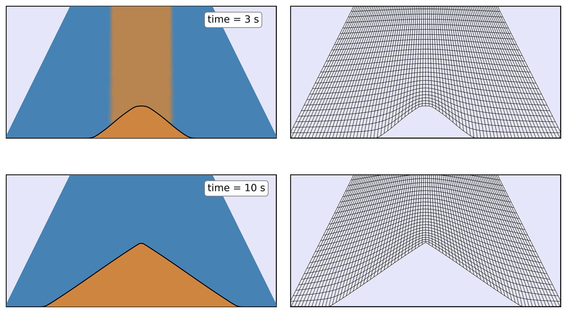
Figure 14 Sediment distribution in the domain at two times during sand deposition in an hourglass. At 3 s, a deposition mound forms from sediment deposited from suspension; at 10 s, all sediment has settled. Left: colors indicate water (blue); right: computational mesh deformation.

Initially, only water is present in the domain. The repose angle is taken equal to β_r=32°. The particles diameter is d=0.29 mm and their density ${\mathit{\rho }}_{\mathrm{s}}=\mathrm{2600}\mathrm{kg}{\mathrm{m}}^{-\mathrm{3}}$. The sediment settling velocity $w_{\mathrm{s}}^{\mathrm{0}}=\mathrm{3.5}\mathrm{cm}{\mathrm{s}}^{-\mathrm{1}}$ is computed using the formula from Fredsoe and Deigaard (1992) (see Table 1) and is considered uniform as the hindrance effect is not taken into account. A constant flux of sediment is injected during 7 s by imposing a constant suspended sediment volume fraction at the top boundary c_s=0.05. The sediment settle under the action of gravity and deposit on the bed. Because the settling is not spatially uniform, pronounced slopes form at the margins of the deposition mound, where avalanching occurs, producing a conical shape similar to that seen in an hourglass. The simulation is then run for 3 more seconds so that all sediment have settled by the end of the simulation (see Fig. 14).

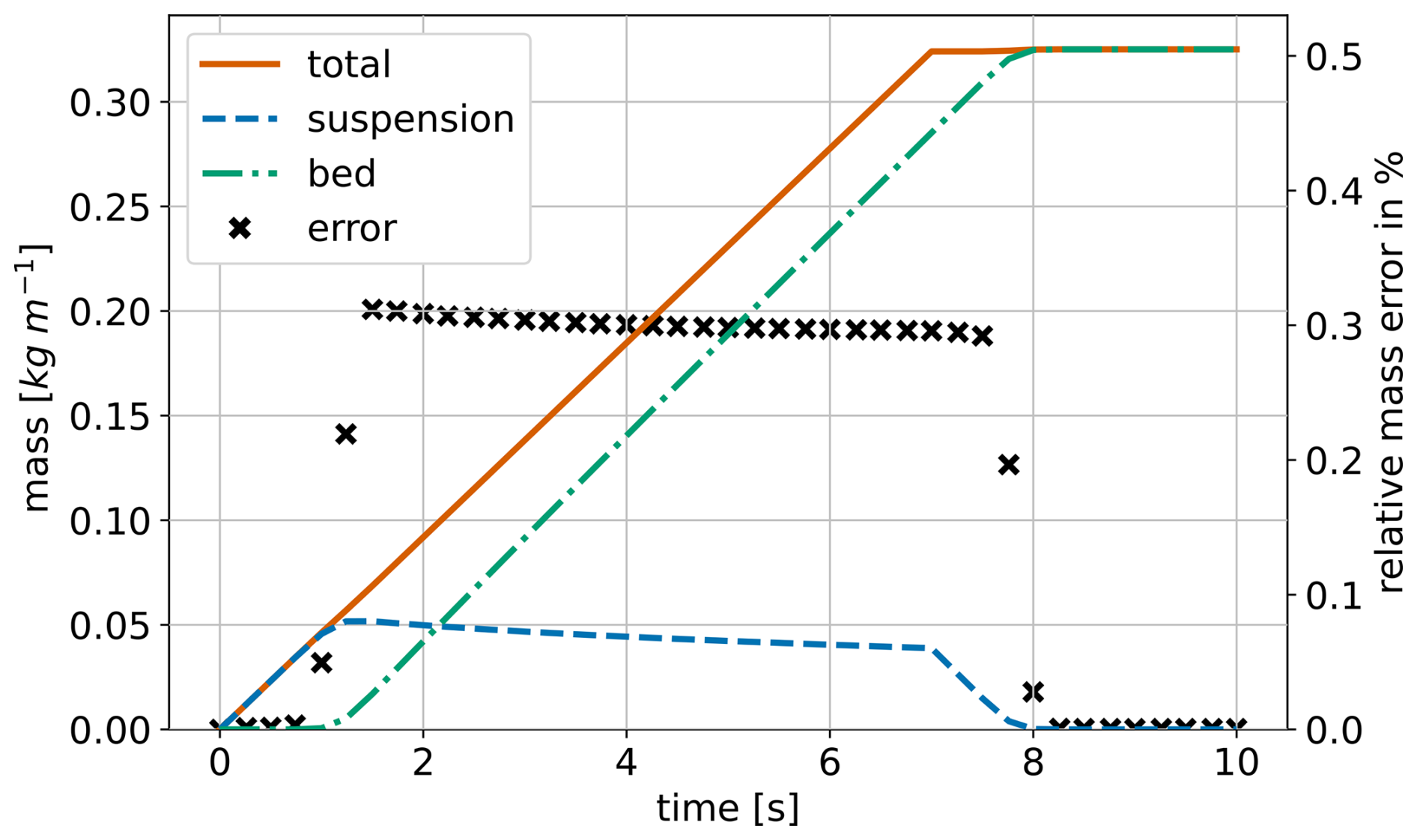
Figure 15 Temporal evolution of sediment mass per unit area, divided into suspended and deposited components, for sand settling in an hourglass. Relative error in total mass (%) is shown by black crosses. Suspended sediment is injected during the first 7 s and fully deposited before the end of the simulation.

The mass repartition of sediments between suspension and deposition is represented in Fig. 15. At the beginning of the simulation, all the sediments are suspended, and their quantity increases linearly over time until t=1.14 s where the sediments start depositing on the bed. As the domain bottom boundary rises, the space occupied by suspended sediments shrinks, leading to a diminution of the mass of suspended sediments. At 7 s, sediment injection into the domain ceases, and approximately one second later, all sediment has settled, with the simulation completing in a few seconds on a single CPU core. Once again, the mass error is evaluated by comparing the mass of sediment, which has been injected into the domain, to the sum of the suspended mass and the bed mass. Just as in the 1D case, the one-time step delay in the bed morphology response induces an error on the total mass in the domain (see Fig. 15). The error subsequently disappears as the sediments settle, thereby verifying mass conservation.

5 Application to dune migration

Sediment transport phenomena often involve bedforms of various scales, ranging from ripples to megadunes, which migrate under the influence of fluid flow. Building on the validation of the model components presented in Sect. 4, this section examines the transport of an isolated dune under a steady current as an illustrative application of sedExnerFoam. First, the experiment used for model comparison is presented, followed by a description of a source term introduced to account for lateral wall friction. The numerical simulation of a dune in a stationary migration regime is presented, where incorporating bedload saturation was necessary to reproduce the migration behavior observed in the experiments. The effects of other model parameters on the simulation results are also briefly discussed. In the third subsection, a 3D simulation is presented using the optimized parameters from the 2D simulations. The purpose of these simulations is to illustrate the numerical model's 3D capability and to identify the current model's limitations.

5.1 Experimental configuration

Different regimes of a lone dune migration over a starved bed have been investigated by Kiki Sandoungout (2019). The author identified the existence of two regimes: the stationary regime and the mass loss scenario. These regimes depend on the flow conditions and on the initial dune mass. In the present work, the focus is on the stationary regime, which exhibits two stages. During the initial phase, the dune morphology evolves rapidly from an initial conical shape formed by sediment deposition in still water. After this transient phase, the dune reaches a stationary state, migrating at a constant speed in the flow direction with minimal deformation.

The experimental facility consists of a hydraulic tunnel working in closed circuit with an experimental section made of a straight channel of length L_c=900 mm, of height H_c=90 mm, and of width W_c=6.03 mm. The flume is closed on the top by a rigid lid. The granular material consists of highly spherical glass beads with a diameter of d=0.4 mm and a density ${\mathit{\rho }}_{\mathrm{s}}=\mathrm{2500}\mathrm{kg}{\mathrm{m}}^{-\mathrm{3}}$. The particle's terminal fall velocity in water is $w_{\mathrm{s}}^{\mathrm{0}}=\mathrm{7.67}\mathrm{cm}{\mathrm{s}}^{-\mathrm{1}}$, which is noticeably higher than values obtained with the models presented in Table 2 ($w_{\mathrm{s}}^{\mathrm{0}}\approx \mathrm{5}\mathrm{cm}{\mathrm{s}}^{-\mathrm{1}}$). The friction velocity upstream of the dune is $u_{*}=\mathrm{2.78}\mathrm{cm}{\mathrm{s}}^{-\mathrm{1}}$ which corresponds to a Rouse number R_o=6.73. This value indicates that bedload is the main transport mechanism for this problem. The critical Shields number (${\mathit{\theta }}_{\mathrm{c}}^{\mathrm{0}}=\mathrm{0.079}$) obtained experimentally is large compared to what is expected from the formulas in Table 2. This could be due to the confinement of the particles in the flume, the ratio of the channel width to the particle diameter being only equal to 16.

In the following, a stationary regime configuration is reproduced numerically. Experimentally, 10 g of particles is introduced through a hole drilled in the channel cover. They deposit under the influence of gravity, forming a conical-shaped mound with slope angles equal to the angle of repose of the granular material. Once the initial pile has formed, a motor is activated to create a left-to-right flow in the test section with a bulk velocity $\stackrel{\mathrm{‾}}{u}=\mathrm{0.43}\mathrm{m}{\mathrm{s}}^{-\mathrm{1}}$. Initially, the particles are loosely packed with a volume fraction of c_s≈0.54 in the particle's bed. As the dune is migrating downstream, the particle bed is compacting, and the sediment volume fraction in the bed increases, resulting in the apparent dune volume decreasing over time until the volume fraction reaches a constant value of about c_s≈0.6.

5.2 2D numerical simulations

Section 5.2 presents the two-dimensional numerical simulations used to reproduce the stationary dune migration regime. It describes the numerical setup, modeling choices, and boundary conditions, and assesses the model’s ability to match the experimental observations. A sensitivity analysis then highlights the key parameters controlling the simulated dune dynamics.

5.2.1 Lateral wall friction modeling

A particularity of these experiments is the thinness of the flume, which makes the lateral wall friction not negligible. The lateral variation of the flow is neglected, and the specific shear stress on the lateral walls τ_wall is computed with the Darcy-Weisbach equation:

$$\begin{array}{}\text{(34)}& {\mathit{\tau }}_{\mathrm{wall}}={\mathit{\rho }}_{\mathrm{f}}f{\displaystyle \frac{\left|\mathit{u}\right|\mathit{u}}{\mathrm{8}}},\end{array}$$

where f is the Darcy-Weissbach friction factor, which can be computed explicitly with the equation from Swamee and Jain (1976):

$$\begin{array}{}\text{(35)}& f={\displaystyle \frac{\mathrm{0.25}}{{\left[{\log }_{\mathrm{10}}\left(\frac{k_{\mathrm{w}}/D_{\mathrm{h}}}{\mathrm{3.7}}-\frac{\mathrm{5.74}}{R{e}_{\mathrm{W}}^{\mathrm{0.9}}}\right)\right]}^{\mathrm{2}}}},\end{array}$$

where $D_{\mathrm{h}}=\mathrm{2}{H}_{\mathrm{c}}{W}_{\mathrm{c}}/(H_{\mathrm{c}}+W_{\mathrm{c}})$ is the hydraulic diameter, k_w the roughness height corresponding to the roughness of the wall, and $R{e}_{\mathrm{W}}=\left|\mathit{u}\right|D_{\mathrm{h}}/\mathit{\nu }$ is the Reynolds number defined with the hydraulic diameter. Integrating the momentum conservation equation (Eq. 1) over the flume width, a new source term F_walls corresponding to the effect of the lateral wall appears:

$$\begin{array}{}\text{(36)}& {\mathit{F}}_{\mathrm{walls}}=-f{\displaystyle \frac{\left|\mathit{u}\right|\mathit{u}}{\mathrm{4}{W}_{\mathrm{c}}}}.\end{array}$$

More details on the derivation of this source term are provided in Appendix C.

In order to confirm the capability of the wall friction term to correctly predict the flow velocity in the narrow flume, five simulations corresponding to different discharges as reported in the experiments are performed. Figure 16 shows a summary of these runs with and without the lateral friction term.

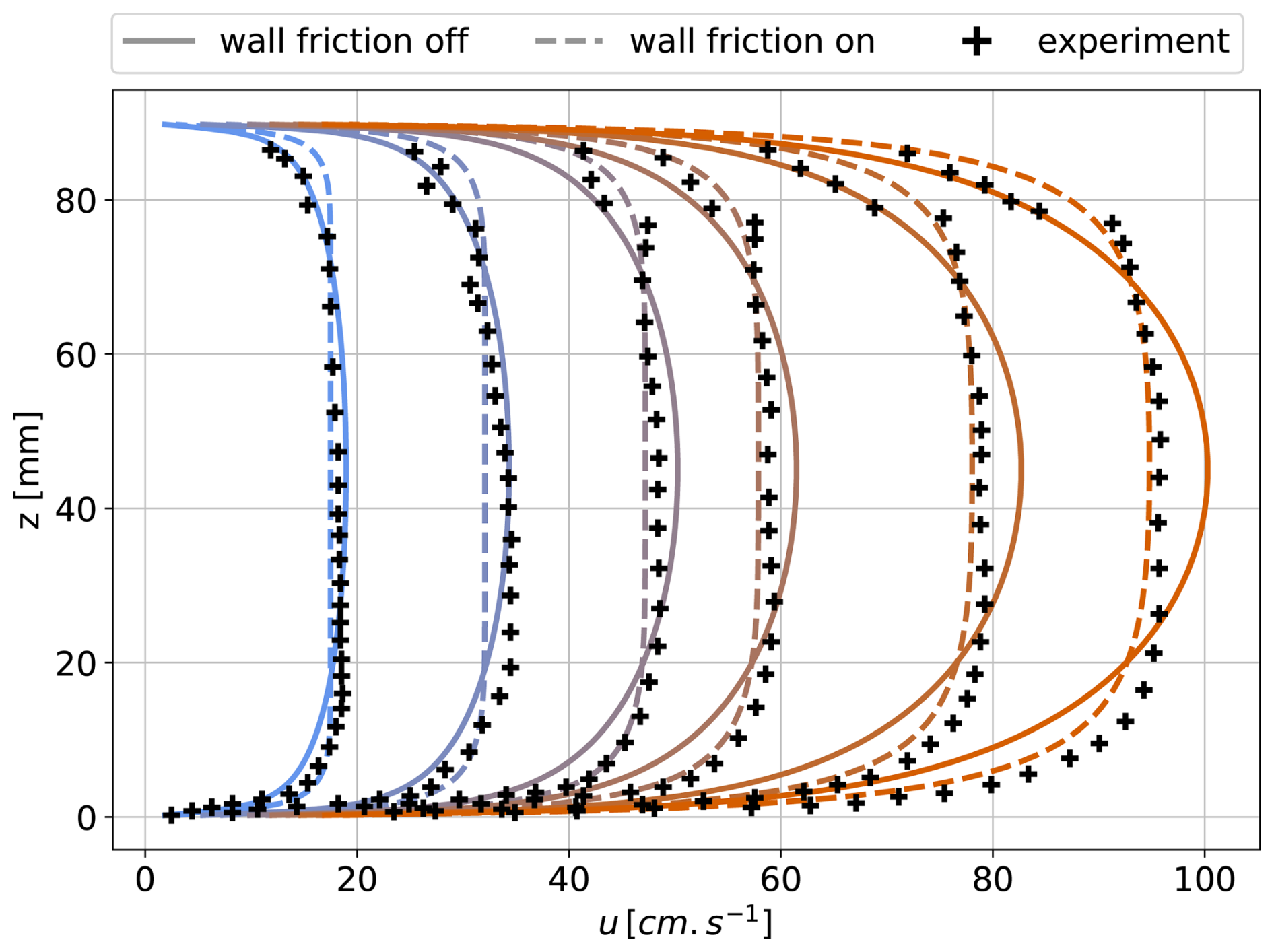
Figure 16 Velocity profiles in the channel in the absence of a dune for different bulk velocities (0.169, 0.309, 0.451, 0.549 and 0.732 m s⁻¹). The solid lines represent profiles obtained without friction on the lateral walls, and the dashed lines represent the one obtained taking into account the lateral friction. The markers are experimental results from Kiki Sandoungout (2019).

Lateral friction leads to a more uniform velocity field as the distance to the upper and lower walls increases, as well as to higher velocity gradients near the boundaries. The agreement with experimental data is improved except at the top of the domain, where the flow is disturbed by the presence of a screw hole, making the data unreliable in this area. The main advantage of accounting for lateral friction as a source term is that it enables the use of a 2D mesh, which significantly reduces the computational cost of the simulation compared with a 3D simulation.

5.2.2 Numerical set-up and model validation

Experimentally, the fluid is initially at rest, and the pump starts to operate at t=0 s, accelerating the flow to the selected mean velocity, $\stackrel{\mathrm{‾}}{u}=\mathrm{0.43}$ m s⁻¹ in the present case. Since the time required for the flow to accelerate and reach the target mean velocity is unknown, an alternative initialization was chosen for the problem. A first simulation of the hydrodynamics without morphological evolution is run for 10 s until the flow over the dune reaches a steady state. The morphological evolution is then activated, and the dune begins to move under the influence of an already fully developed flow. Regarding the initial condition, as the variation in particle volume fraction in the bed, observed in the experiments (see Sect. 5.1), cannot be reproduced by the present model (the bed porosity is considered a constant over space and time), it was chosen to initialize the dune with a volume corresponding to the one at the end of the experiment and not the initial one. As a result, the initial dune geometry in the numerical simulations is initially slightly smaller than the experimental one, but their volumes match after a few seconds, once the granular material has compacted in the experiments.

The inlet boundary conditions are imposed as follows: a uniform velocity is applied $\stackrel{\mathrm{‾}}{u}=\mathrm{0.43}$ m s⁻¹; Dirichlet boundary conditions are used for the turbulent quantities: k=0.001 m² s⁻² and ω=15 s⁻¹. It corresponds to a turbulent intensity $I_{\mathrm{t}}=\sqrt{\frac{\mathrm{2}}{\mathrm{3}}k}/\stackrel{\mathrm{‾}}{u}=\mathrm{0.06}$. Those values were chosen after simulating the flow in the flume without particles, and it has been verified through a sensitivity analysis of the upstream domain length that the solution does not change when using a longer domain (not shown here). The top boundary is a rigid wall, and a no-slip boundary condition is applied on the velocity field. At the outlet, a zero gradient condition is applied to all fields except the fluid pressure, for which a homogeneous Dirichlet condition is prescribed. The numerical schemes used to discretize the different terms in the momentum equations (Eq. 1) are: a backward scheme for the temporal derivative, a second-order linear-upwind scheme for the advection term, and a linear scheme for the diffusion terms. The same schemes are used for the advection-diffusion equation of the suspended sediment concentration, except for the advection, for which a first order upwind scheme has been used to ensure the boundedness and positivity of the sediment concentration. The numerical schemes for the Exner equation are: Adams-Bashforth 2nd order in time, upwind first order for the bedload, and a linear scheme for the avalanche. The bedload flux saturation equation has been integrated using an explicit Euler scheme for the time derivative, and discretized using a first-order upwind scheme for the saturation length term. A sensitivity to the saturation length and time values will be presented in Sect. 5.2.3. All the numerical results presented in this subsection have been obtained using a saturation length L_sat=5 mm and saturation time T_sat=0.01 s.

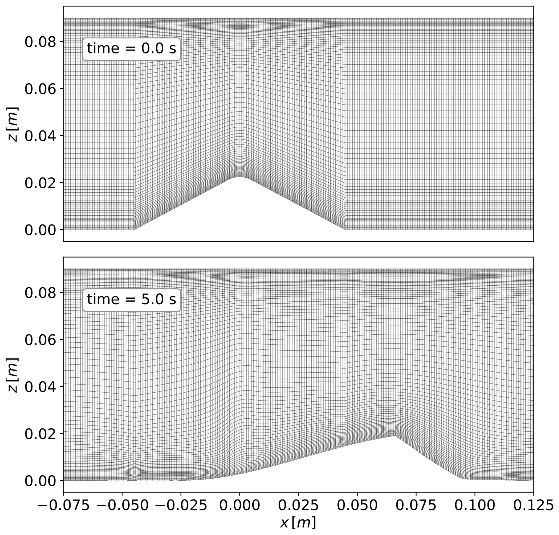
A grid convergence study has been performed for the hydrodynamic simulations, and the details are provided in Appendix D. The finest grid has been retained for the numerical results presented in this subsection, with the following parameters: $n_x\times n_z=\mathrm{1100}\times \mathrm{80}$, the first grid cell center distance to the wall in the straight channel region is equal to $z_{\mathrm{1}}=\mathrm{1.42}\times {\mathrm{10}}^{-\mathrm{4}}$ m. A visualization of the mesh at two different times during the dune migration process is presented in Fig. 17.

Figure 17 Representation of the dune mesh at different times during the migration process.

The numerical simulation results are illustrated in Fig. 18, which shows the fluid flow at three different times using an optimized set of parameters that will be described in Sect. 5.2.3.

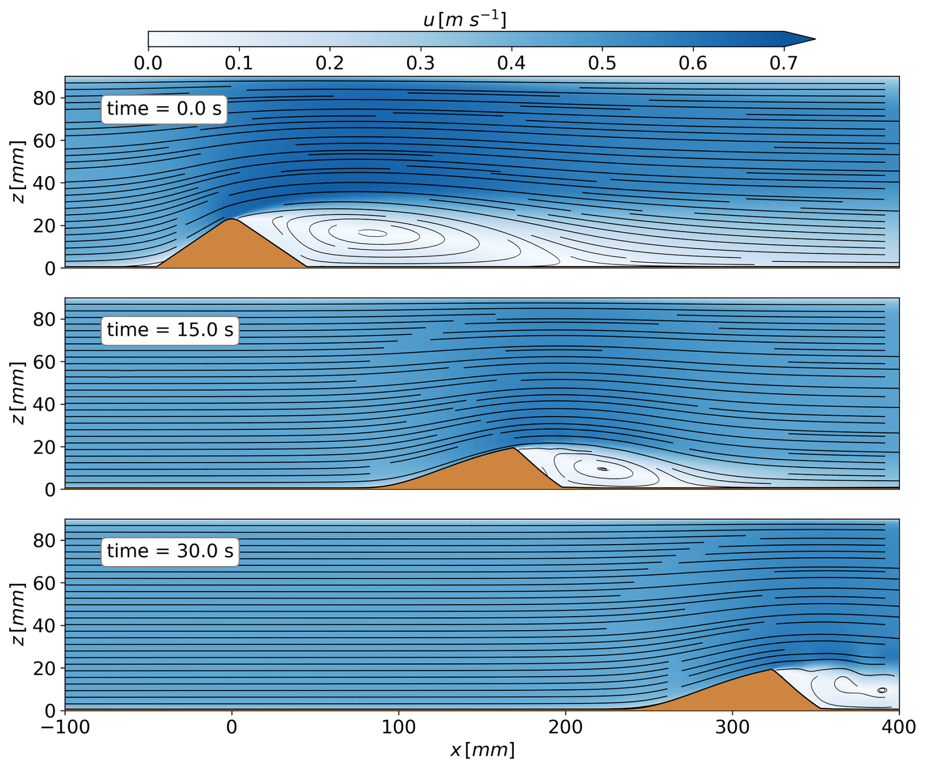
Figure 18 Representation of the dune at different times (0, 15, and 30 s) during the migration process. The flow streamlines highlight flow detachment near the dune crest and the recirculation cell downstream. Starting from an initial conical shape, the dune evolves into an asymmetric stationary form.

In order to compare the results more quantitatively, Fig. 19 shows the numerical and experimental dune profile at four times, 0, 4, 8 and 12 s. As can be seen from this figure, the dune morphology agrees fairly well with the experimental data. The dune shape does not change much between 8 and 12 s, in agreement with the stationary regime observed experimentally.

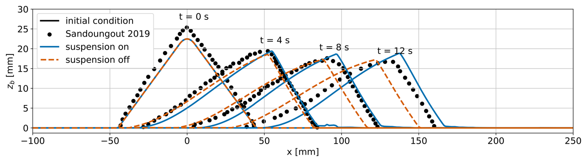
Figure 19 Sediment bed elevation at different times, 0, 4, 8, and 12 s. Comparison between the results from two simulations and experimental results. The simulations use the same mesh, same parameters, but for one, the suspended load is not taken into account.

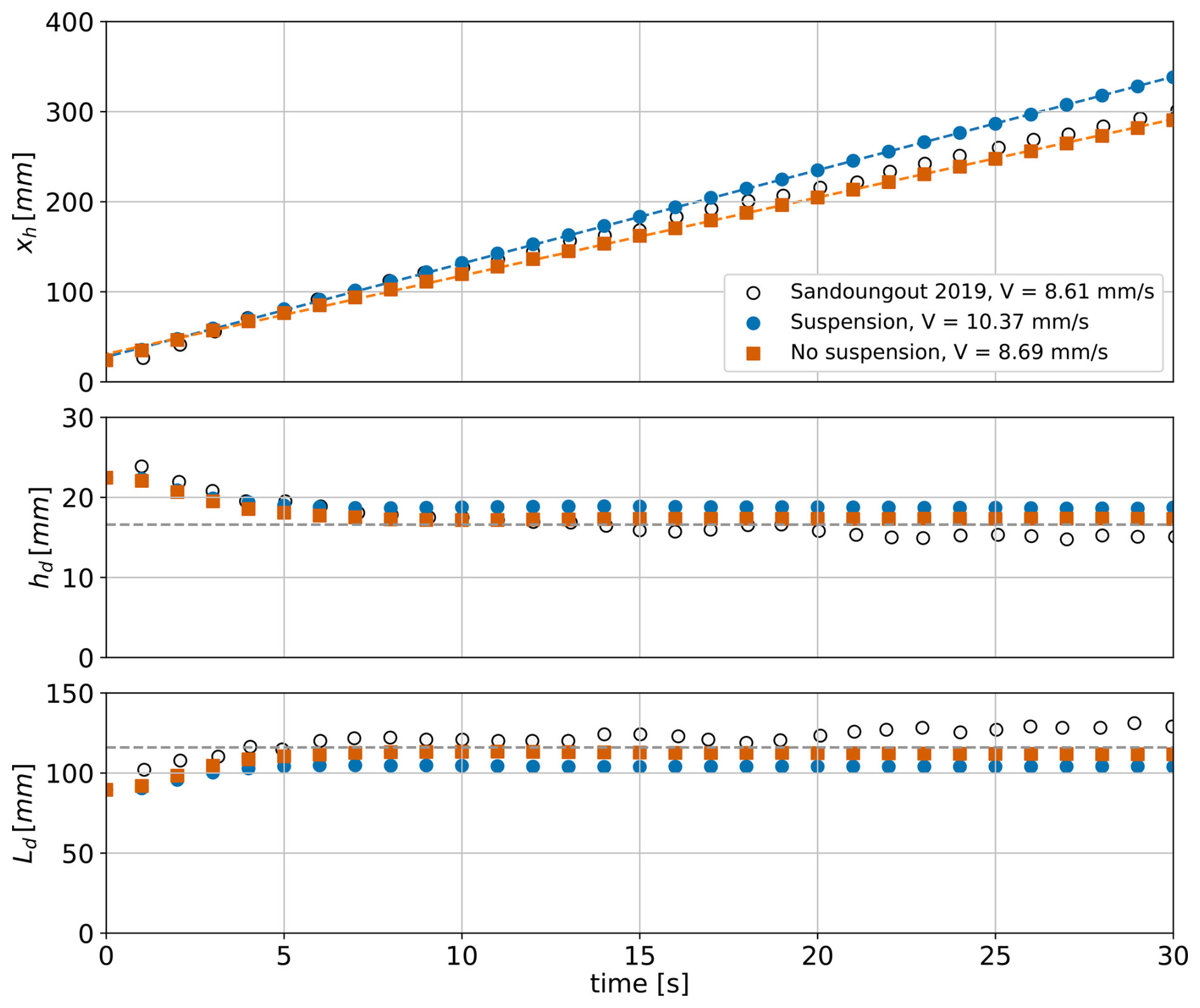
Figure 20 Dune morphological parameters evolution in time. From top to bottom are plotted the dune position represented by the coordinates x_h, which is located halfway up the downstream face of the dune, as well as the dune height h_d and the dune length L_d. In the top panel, the dashed lines represent the linear fit of the numerical results from which the dune migration speed is estimated as the slope of the linear regression.

The dune morphological parameters over time, which are the dune position, its height, and length, are presented in Fig. 20. The dune position is characterized by the coordinate x_h located at mid-height on the downstream slope of the dune. The dune height and length are estimated from the base of the triangle formed by two straight lines fitted on the dune upstream and downstream slopes (see Appendix D for details). Two simulations with and without considering the suspended load transport are shown. As expected, because of the high value of the Rouse number (R_o>6), the suspension has little effect on the dune evolution. Its height and length in the stationary regime remain unchanged, and regarding the migration velocity, only a small difference is observed, 10.37 and 8.69 mm s⁻¹ for simulations with and without considering the suspended load, respectively. This migration speed difference is also observed in Fig. 19, showing the bed elevation profiles at different times. In the configuration with suspended load, part of the suspended sediment passes over the dune and settles within the recirculation zone, creating the artifacts observed downstream of the dune. These deposits are subsequently re-integrated by the dune as it migrates downstream. Overall, the numerical model is able to reproduce the dune migration and evolution correctly, but some discrepancies are still observed. The crest of the dune is sharp in both numerical simulations compared to the experiment, and as a result, the height of the dune is slightly overestimated (see Fig. 20). At the same time, the length of the dune seems to be underestimated, but it could also be a consequence of the method used to estimate the dune length (see Appendix D). The two stages of the dune migration are clearly observed in the numerical results. During the first 10 s, the dune shape changes rapidly, its height decreases, and its length increases. At 10 s, the dune has reached a stationary stage, and its shape remains unchanged as it migrates at a constant speed. All these results validate sedExnerFoam for this 2D vertical application. As mentioned earlier, the simulations presented above have been obtained by optimizing some of the model parameters, and the sensitivity to the most important ones will be described in the following subsection.

5.2.3 Sensitivity analysis and bedload flux saturation effect

A first parameter that significantly affects the numerical results is the grid resolution and, in particular, the near-bed resolution in the areas where the flow is highly non-uniform. In the present configuration, it corresponds to the upstream slope of the dune where the flow is accelerated up to the crest. Downstream of the crest, the flow detaches and generates a recirculation cell on the lee side, as illustrated in Fig. 18. A poor near-bed mesh resolution leads to an underestimation of the bed shear stress (see Appendix D) and, consequently, to a slower dune migration. The distance in wall units between the cell centers of the first layer and the bed boundary is maintained between $z^{+}=\mathrm{1}$ and $z^{+}=\mathrm{5}$ in the present simulations. The choice of the numerical scheme used to discretize the advection term in the momentum equation (Eq. 1) also significantly affects the dune shape. This is mainly due to the influence of this numerical scheme on the recirculation cell on the lee-side and to the position of the detachment point, which is located upstream of the dune crest for high-order advection schemes but downstream of the dune crest when using a low-order upwind scheme. When the flow detachment occurs downstream of the dune crest, the dune shape was found to take a rounder shape, not matching the experimental measurements.

Another sensitive parameter in this configuration is the critical Shields number ${\mathit{\theta }}_{\mathrm{c}}^{\mathrm{0}}$, which is evaluated in the range 0.033–0.046 by the different models presented in Table 2 but was experimentally estimated at a higher value of 0.079. Increasing the value of ${\mathit{\theta }}_{\mathrm{c}}^{\mathrm{0}}$ not only slows down the dune but also reduces its height and length in the stationary regime. An intermediate value of ${\mathit{\theta }}_{\mathrm{c}}^{\mathrm{0}}=\mathrm{0.05}$ was found to yield good results. In addition, the critical Shields number was corrected with the local slope according to Eq. (13). A final key modeling choice is the formula used to calculate bedload transport. It was found that the formulas presented in Table 2 were all predicting dune velocity at least two times slower than the one observed experimentally. Therefore, a custom bedload formula ${\mathit{\varphi }}_{\mathrm{b}}=\mathrm{32}{\mathit{\theta }}^{\mathrm{1}/\mathrm{2}}\mathit{\varpi }(\mathit{\theta }-{\mathit{\theta }}_{\mathrm{c}})$ was used. It corresponds to an intensified version of the formula from Nielsen (1992) and can be considered reasonable in view of the significant scatter associated with bedload measurements (Recking, 2010). Indeed, even if these formulations are commonly used to model sediment transport in a variety of flow conditions, they are empirical relations derived from data of uniform flows in a straight channel. Therefore, they may not precisely describe sediment transport in accelerated flow regions, recirculation cells, and other non-uniform flows. It shall also be recalled that the present configuration corresponds to a very narrow channel, which may also affect the sediment transport fluxes.

The most critical and original mechanism that is accounted for in the present model is the bedload flux saturation, which represents the particle's inertia with respect to the fluid flow. To illustrate the sensitivity to the saturation length and time, the results of seven simulations obtained with the same numerical set-up except for L_sat and T_sat are presented in Fig. 21, which shows the bed level after 10 s of migration. The saturation length L_sat value is varied from 1.25 to 20 mm while the saturation time T_sat value is varied from 0.005 to 0.2 s. The green curve corresponds to the optimized configuration shown in Sect. 5.2.2. The pink curve shows the smallest L_sat value that the model could withstand without crashing. The numerical results indicate that introducing a finite saturation length accelerates the migration process up to a value of about L_sat =0.0025 m here, above this value the dune migration speed is slowed down (see orange and blue dashed lines). For the largest L_sat value tested here, L_sat=0.02 m, the T_sat has been increased to 0.02 s as the simulation crashed with T_sat=0.01 s. Three simulations have been performed for the same saturation length L_sat=0.005 m and for three values of T_sat=0.005, 0.01, and 0.02 s. In this range, no effect of the saturation time T_sat on the dune migration has been observed, and the value of T_sat=0.01 s has been retained.

Saturation acts as a spatial filter, and it smooths out the maximum of q_sat. For very large values of L_sat, this results in an underestimation of q_b, and the migration velocity is reduced. For very low values of L_sat, the dune shape is very strange, and the migration speed is too low. In the following, an explanation of what is happening in this limit of very small or even zero saturation length is provided. On the upstream slope of the dune, the flow is accelerated, and the bed shear stress increases downstream (see Fig. D2 in Appendix D). The bed shear stress exhibits a maximum slightly upstream of the crest, driving the dune growth. At the position where the flow detaches, the shear stress value suddenly drops. If the inertia of the bedload, the bedload flux saturation, is not accounted for, then the sediments accumulate at the crest, and the dune height increases rapidly (Charru et al., 2013). At some point, the upstream slope becomes steeper than the angle of repose, and the avalanche flux compensates for the shear-driven bedload flux. The dune then stops moving and stays stuck in a nonphysical state (see pink line in Fig. 21). In reality, the sediments arrive at the crest with a certain velocity, and some distance is needed for them to adapt to the sudden change in bed shear stress. They could even “take off” into suspension due to the abrupt change of slope at the crest of the dune. To retrieve a realistic behavior of the dune migration compared with the experiment, our model and simulations suggest using the saturation of the bedload flux (Eq. 16) as an important physical process to take into account. This is in line with recent improvements made by physicists in the understanding of bedform dynamics (e.g. Charru et al., 2013). According to Charru et al. (2013), for underwater transport, the saturation length is controlled by particle's settling and can be expressed as: $L_{\mathrm{sat}}\propto u_{*}/w_{\mathrm{s}}^{\mathrm{0}}\times d$, and for aeolian transport, the saturation length is dominated by particles' inertia and can be expressed as: $L_{\mathrm{sat}}\propto {\mathit{\rho }}_{\mathrm{s}}/{\mathit{\rho }}_{\mathrm{f}}\times d$. The first estimate leads to a value of about L_sat≈3 mm while the latter leads to a value of about L_sat≈1 cm, in agreement with the values tested herein. Nevertheless, some numerical stability issues have been observed that are not yet fully understood and explained, and deserve further work in the near future.

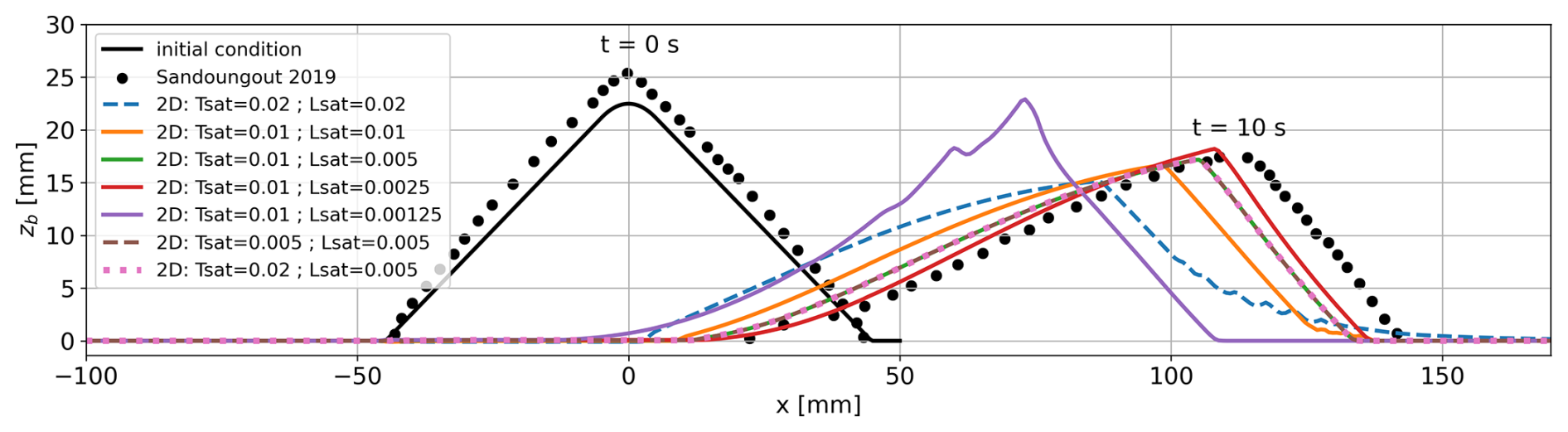
Figure 21 Bed elevation obtained with different saturation length values, ranging from L_sat=1.25 mm to L_sat=20 mm with saturation time T_sat=0.01 s except for L_sat=20 mm where T_sat=0.02 s (due to numerical stability condition) and 2 configurations with T_sat=0.005 s and T_sat=0.02 s with L_sat=5 mm are also showed. All these configurations have been performed without suspension to limit potential non-linear interactions between bedload and suspended load on the dune migration.

5.2.4 Partial conclusion on the 2D simulations

The results presented in this section demonstrate the sedExnerFoam model's ability to handle complex hydromorphodynamic coupling. It has been shown that grid resolution, particularly in the near-wall region, is important for the quality of simulation results. In particular, predictions of bed shear stress are sensitive to grid resolution. The decision was made to use very refined grids, which resulted in a significant CPU cost. The current implementation takes approximately four hours of wall-clock time on a single CPU core to simulate 15 s of morphodynamics in two dimensions with saturation and without suspension. Saturation of the bedload flux is a novel concept in the context of a 3D computational fluid dynamics solver coupled with an Exner model. The results presented here suggest that further work is required on the physical aspects and numerical implementation. This includes the choice of values for the L_sat and T_sat parameters, the choice of numerical schemes, and associated stability issues. In particular, it is worth considering whether the model can simulate three-dimensional problems. This is the topic of the following subsection.

5.3 3D numerical simulations

Section 5.3 presents three-dimensional numerical simulations of the dune migration problem to assess the model’s performance. The 3D setup is derived from the 2D case and applied under the same physical and numerical assumptions. The results are compared with the 2D simulations to evaluate consistency, robustness, and computational performance.

The grid of the 2D case presented in the previous section is just extruded in the y-direction to match the experimental channel width (W_c=6 mm) using 10 cells. This resolution allows us to maintain an aspect ratio close to unity between the streamwise and spanwise grid sizes (Δx≈0.72 mm, Δy≈0.6 mm). A grid resolution of n_x=1100, n_y=10, and n_z=80 is employed, corresponding to 880 000 cells. The numerical schemes and empirical parameters used in the sediment transport model for the 3D configuration are identical to those employed in the 2D case. It should be noted that the lateral wall boundary conditions are set as symmetry planes, while the source term accounting for lateral wall friction remains active in the present simulations.

The results of the 3D simulations with suspension are shown in Fig. 22 at three different times during the migration process: t=0, 5 and 10 s. In this figure, the flow streamlines are colored according to their velocity magnitude. Also shown is a color plot of the suspended concentration, c_s, in a vertical plane at y=0.006 m on a log scale. The color plot on the bed patch represents the q_sat, and the bed grid is illustrated by the white lines. As shown in the figure, the flow recirculation cell downstream of the dune is clearly visible. The size of the cell reduces as the dune migrates and its height decreases. The suspended load region encompasses the entire recirculation cell, with a solid volume fraction ranging from 10⁻³ to 10⁻². This seems to be an overestimation compared to the experimental observations made by Kiki Sandoungout (2019). Not much oscillation is observed at the bed, except perhaps at the downstream toe of the dune, where suspended particles accumulate due to the recirculation cell. This confirms the robustness of the numerical implementation for two-dimensional bathymetry. One final observation is the repartition of the q_sat, which shows a clear maximum near the crest of the dune. It may be difficult to discern from this figure, but the maximum actually occurs at the crest at t=5 s and t=10 s in the stationary migration regime. This is consistent with the physical arguments presented, for example, in Charru et al. (2013), who argue that saturation of the bedload flux constitutes the stabilizing mechanism for bedform growth. A bedform's maximum amplitude is reached when the maximum occurs at the crest.

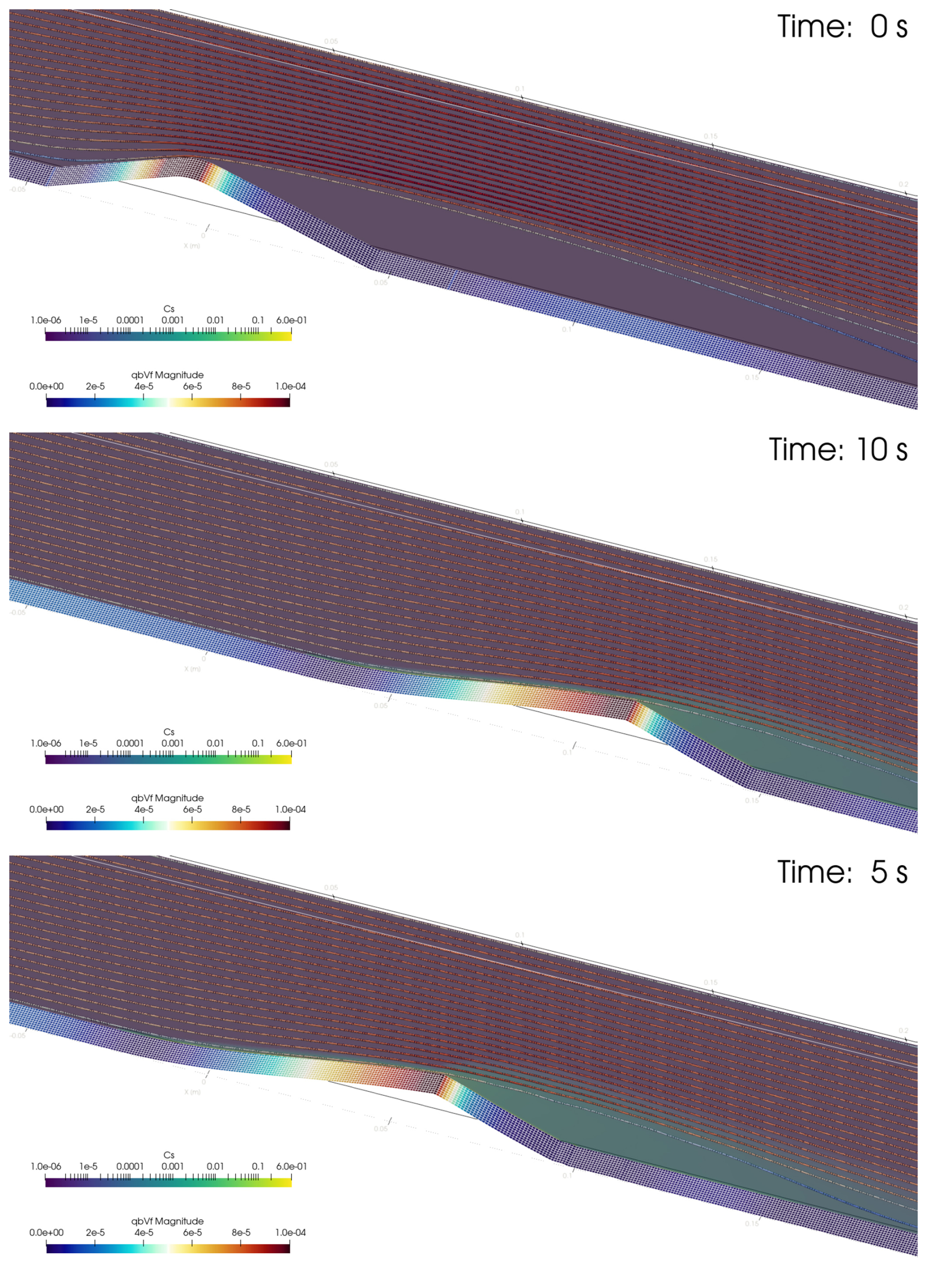
Figure 22 Representation of the dune and the flow streamlines of the 3D configuration at different times, t=0, 5 and 10 s from top to bottom, during the migration process. The colorplot at the bed represents the saturated bedload flux q_sat (L_sat=0.005 m and T_sat=0.01s), and the colorplot in a vertical plane represents the suspended concentration c_s in log scale. The streamlines are colored by the flow velocity.

Figure 23 shows a comparison of the bed profiles at different times during the migration process (t=0, 4, 8, and 12 s). The results are compared with the 2D case shown in the Fig. 19. The differences between the two configurations are very small, demonstrating the reliability of the 3D implementation of the numerical model. The 3D simulation results without suspension exhibit small oscillations of the bed elevation on the stoss side of the migrating dune at t=12 s. These oscillations do not degenerate into numerical instabilities. This is likely due to the use of an upwind scheme for the divergence of the bedload flux in the solution of the Exner equation. The model also has a centered scheme for this term; it runs smoothly in the 2D case but crashes in the 3D case, as illustrated in Fig. D3 in Appendix D. Further work is needed to improve the accuracy and the stability of the coupling between hydrodynamics, sediment transport (including bedload flux saturation), and the morphological evolution. This includes developing a filter for the bed evolution increment (e.g. Jacobsen, 2011), developing high-order, non-oscillating schemes, such as WENO or NOCS (e.g. Guerin et al., 2016; Marieu et al., 2008), and/or using a predictor-corrector algorithm for the Exner equation solution.

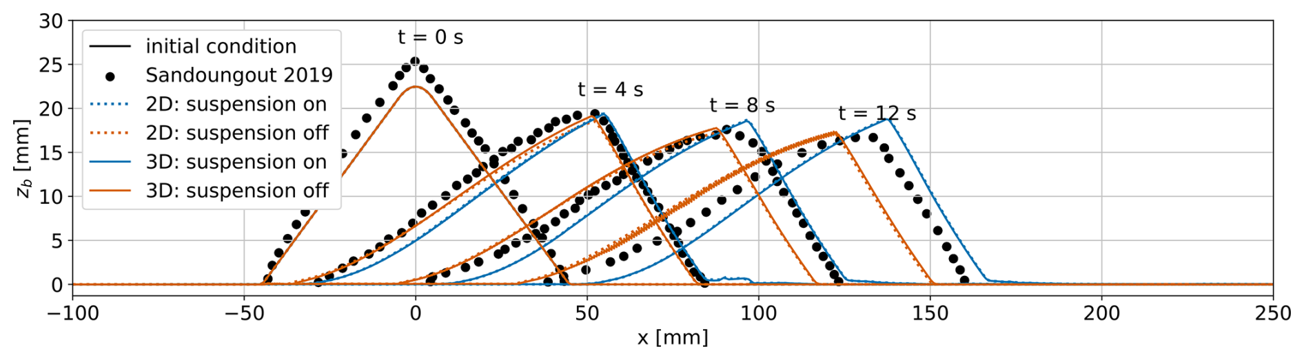
Figure 23 Sediment bed elevation at different times, 0, 4, 8, and 12 s. Comparison between the results from 2D and 3D simulations with and without suspension and experimental results.

The hydrodynamic part of the model benefits from the native parallelization available in OpenFOAM. However, the Exner solver is currently only available sequentially. One workaround for running parallel simulations is to decompose the numerical domain while ensuring that all the bed cells remain on a single CPU core. While not optimal, this method enables 3D simulations to be performed in a reasonable amount of time. To demonstrate the performance of sedExnerFoam, the 3D simulation without suspension presented in this subsection took 1 h and 53 min on 32 CPU cores to simulate 5 s of physical time. This performance is acceptable compared to the 2D case run on a single CPU core. Nevertheless, parallelizing the Exner solver will be necessary to take full advantage of the OpenFOAM parallelization capabilities.

6 Discussion

The newly developed solver, sedExnerFoam, shares several characteristics with existing three-dimensional morphodynamic models (e.g. Liu and García, 2008; Jacobsen et al., 2014; Jacobsen and Fredsoe, 2014; Baykal et al., 2015), while incorporating a number of methodological and numerical developments. These include the use of a single deforming mesh for both hydrodynamics and suspended sediment transport, enabled by a near-wall diffusivity formulation, as well as the introduction of a saturation length in the bedload flux formulation to account for sediment inertia. Within the range of models considered by the authors, the inclusion of bedload flux saturation is not commonly implemented in three-dimensional subaqueous morphodynamic solvers and is shown to be essential for accurately reproducing observed dune migration and crest dynamics in the configurations examined.

A further strength of sedExnerFoam is its modular, object-oriented structure, which allows users to select and modify closures for settling velocity, bedload transport, the critical Shields number, and avalanching processes. This flexibility is supported by the solver’s open-source availability and the adoption of continuous integration testing, which contribute to transparency, reproducibility, and long-term maintainability. In addition, the avalanche model implemented here avoids the iterative procedures commonly employed in existing three-dimensional morphodynamic models, while the near-wall diffusivity formulation enables the use of a single computational mesh for both flow and suspended sediment transport.

Despite these advantages, several limitations remain. The current bed boundary condition for erosion and deposition may lack robustness for large-scale flows, and further development is required to extend the model scope to engineering-scale applications. Moreover, the feedback of suspended sediment on flow hydrodynamics is neglected. Accurate estimation of bed shear stress requires very fine mesh resolution in regions of strongly non-uniform flow, while the mesh deformation solver and the sensitivity of the Exner equation to spurious bed oscillations impose additional constraints on numerical robustness.

In comparison with existing morphodynamic models, sedExnerFoam occupies an intermediate position between large-scale three-dimensional morphodynamic models – such as openTELEMAC (Galland et al., 1991) and Delft3D (Lesser et al., 2004) – and fully resolved two-phase flow approaches, including Eulerian–Eulerian (e.g. Chauchat et al., 2017) and Eulerian–Lagrangian (e.g. Cheng et al., 2018) formulations. Large-scale models are well-suited for reach-scale river simulations but generally lack the spatial resolution required to represent fine-scale interactions with obstacles such as bridge piers, and often rely on simplified turbulence closures and near-wall modelling compared to CFD-based frameworks such as OpenFOAM. These limitations must be considered alongside the increased computational cost associated with the finer grids and smaller time steps typically required by sedExnerFoam. Within this context, the solver is designed to resolve coupled flow–structure–bed interactions that are relevant to scour processes and bedform dynamics.

At the opposite end of the modelling spectrum, two-phase flow approaches provide a more detailed representation of sediment transport physics but at a substantially higher computational cost. For instance, Nagel et al. (2020) reported that three-dimensional two-phase RANS scour simulations using sedFoam required approximately 108 000 CPU hours to simulate 600 s of physical time. The combined use of two-phase flow models and sedExnerFoam may therefore support the development and assessment of sediment transport closures, for instance, through the Exner diagnosis method proposed by Gilletta et al. (2026). More generally, each modelling approach is suited to a specific range of spatial and temporal scales, and the availability of open-source tools spanning this range is expected to benefit the scientific community by facilitating cross-comparisons and reducing uncertainty in morphodynamic simulations. In this context, sedExnerFoam is intended to contribute as an intermediate-scale modelling tool and to support upscaling approaches such as those presented previously.

7 Summary and outlook

This study presents a new numerical solver, sedExnerFoam, designed to investigate sediment transport and morphological evolution. Developed within OpenFOAM^® (v2412) and based on the pimpleFoam framework, the solver incorporates a wide range of closures for particle settling velocity, bedload transport, and the critical Shields number. These closures can be readily modified by the user, taking full advantage of the object-oriented architecture of OpenFOAM.

The model has been extensively validated against analytical solutions and experimental data through a series of benchmark tests spanning a wide range of applications, including turbulent suspensions in open-channel flows, idealized dune migration, sand deposition, and mass conservation in hourglass configurations. These benchmarks were deliberately selected to isolate and evaluate individual model components. Finally, the application to the migration of an isolated dune under steady flow conditions demonstrates the solver’s capability to handle complex coupled processes involving flow separation, avalanching, and significant mesh deformation.

The major innovations in sedExnerFoam are: (i) the avalanche model that eliminates the need for non-physical and computationally expensive iterative procedures commonly used in existing three-dimensional morphodynamic solvers; (ii) the introduction of near-wall turbulent diffusivity for suspended sediment transport, which enables the use of a single mesh for both hydrodynamics and sediment concentration and (iii) the incorporation of bedload flux saturation which is unique among subaqueous sediment transport models to the best of the authors’ knowledge. The main strengths of sedExnerFoam lie in its open-source availability, extensive validation on idealized benchmarks, and robust software development practices. Continuous integration testing within the GitHub repository supports long-term maintenance and backward compatibility. Future work will focus on improving the robustness of the bed boundary condition for erosion and deposition and enhancing computational efficiency, particularly through improved parallelization of the Exner equation. The implementation of filtering techniques and/or high-order non-oscillatory schemes for bed evolution may further reduce numerical instabilities while preserving morphological accuracy. Additional developments could include the treatment of free-surface effects, multiple grain-size classes, and cohesive sediments.

In the longer term, sedExnerFoam is intended to be used in conjunction with sedFoam (Chauchat et al., 2017), a two-phase flow sediment transport model. This combined approach aims to derive more accurate and robust sediment transport closures through systematic upscaling from two-phase flow simulations.

Appendix A: Abbreviations and notations

Abbreviations
ALE	Arbitrary Lagrangian Eulerian
CFD	Computational Fluid Dynamics
DNS	Direct Numerical Simulation
FAM	Finite Area Method
FVM	Finite Volume Method
IBM	Immersed Boundary Method
LES	Large Eddy Simulation
RAS	Reynolds-Averaged Simulation
RMSE	Root Mean Square Error
SMAPE	Symmetric Mean Absolute Percentage Error
SST	Shear Stress Transport
TKE	Turbulent Kinetic Energy
Notations
cs	Suspended sediment volume fraction
$c_{\mathrm{s}}^{\max }$	Maximum sediment volume fraction
$c_{\mathrm{b}}^{*}$	Reference concentration
$c_{\mathrm{b},\max }^{*}$	Maximum reference concentration
CD	Drag coefficient
d	Diameter of the sediment [m]
D	Deposition rate [m s−1]
Dh	Hydraulic diameter, 4 times the ratio of the wet area to the wet perimeter [m]
D*	Dimensionless sediment diameter
E	Erosion rate [m s−1]
eg	Unit vector oriented with gravity
f	Darcy-Weissback friction factor
Fh	Hindrance function
Fwalls	Side walls friction source term [m s−2]
F1	First blending function of the k−ω SST model
F2	Second blending function of the k−ω SST model
F3	Third blending function of the k−ω SST model
g	Gravity acceleration [m s−2]
hd	Dune height [m]
k	Specific turbulent kinetic energy [m2 s−2]
ks	Nikuradse equivalent roughness height [m]
$k_{\mathrm{s}}^{+}$	Roughness Reynolds number
kw	Wall equivalent roughness height [m]
Ld	Dune length [m]
Lsat	Saturation length [m]
lsb	Distance to the sediment bed boundary [m]
p	Pressure of the fluid [$\mathrm{kg}{\mathrm{m}}^{-\mathrm{1}}{\mathrm{s}}^{-\mathrm{2}}$]
P	Specific turbulent kinetic energy production rate [m2 s−3]
qav	Avalanche related bedload flux [m2 s−1]
$q_{\mathrm{av}}^{\mathrm{0}}$	Maximum avalanche related bedload flux [m2 s−1]
qb	Bedload flux [m2 s−1]
qsat	Saturated bedload flux [m2 s−1]
Ro	Rouse number, ratio of the settling velocity to the upwards velocity of the grains

s	Ratio of sediment density to fluid density
S	Strain rate tensor [s−1]
SR	Roughness coefficient in rough wall functions for ω
t*	Breaking time [s]
Tsat	Saturation time [s]
u	Fluid velocity field [m s−1]
u′	Fluctuating velocity field [m s−1]
u*	Friction velocity [m s−1]
Vf	Volume of fluid [m3]
Vs	Volume of sediment [m3]
ws	Settling velocity of suspended sediment [m s−1]
$w_{\mathrm{s}}^{\mathrm{0}}$	Terminal settling velocity of a lone particle in a quiescent fluid [m s−1]
zb	Sediment bed elevation [m]
αs	Angle between the steepest slope direction and the shear direction
βr	Repose angle of the granular material
βs	Bed slope angle
Γc	Mesh diffusivity [m2]
δzb	Bed elevation increment [m]
$\mathit{\delta }{z}_{\mathrm{b}}^{*}$	Reference level [m]
ΔXc	Cell center displacements [m]
ϵ	Dissipation rate of turbulent kinetic energy [m2 s−3]
ϵs	Turbulent diffusivity for suspended sediment [m2 s−1]
ϵw	Additional near bed diffusivity for suspended sediment [m2 s−1]
${\mathit{ϵ}}_w^{\mathrm{0}}$	Constant in the near bed diffusivity definition
θ	Shields number, dimensionless bed shear stress
θc	Critical Shields number with slope correction
${\mathit{\theta }}_{\mathrm{c}}^{\mathrm{0}}$	Critical Shields number on a flat bed
κ	Von Kármán constant
λs	Porosity of the granular material
μs	Static friction coefficient
ν	Kinematic viscosity of the fluid [m2 s−1]
νt	Turbulent eddy viscosity [m2 s−1]
ξw	Constant in the near bed diffusivity definition
ρf	Density of the fluid [kg m−3]
ρs	Density of the sediment [kg m−3]
σc	Schmidt number, ratio of eddy viscosity to turbulent diffusivity of suspended sediment
τb	Shear stress exerted on the bed [$\mathrm{kg}{\mathrm{m}}^{-\mathrm{1}}{\mathrm{s}}^{-\mathrm{2}}$]
τf	Filtering tensor in Navier-Stokes equation [m2 s−2]
τwall	Lateral wall friction [$\mathrm{kg}{\mathrm{m}}^{-\mathrm{1}}{\mathrm{s}}^{-\mathrm{2}}$]
ϕb	Einstein number, dimensionless bedload flux
ω	Specific dissipation rate of turbulent kinetic energy [s−1]

Appendix B: RANS k-ω SST model

The blending function F₁ is defined as follows:

$$\begin{array}{}\text{(B1)}& \begin{array}{rl}{F}_{\mathrm{1}}& =\tanh \left[min\left(min\left(max\left({\displaystyle \frac{\sqrt{k}}{{\mathit{\beta }}_{*}\mathit{\omega }y}},{\displaystyle \frac{\mathrm{500}\mathit{\nu }}{\mathit{\omega }{y}^{\mathrm{2}}}}\right),\right.\right.\right.\\ & \left.{\left.\left.{\displaystyle \frac{\mathrm{4}{\mathit{\alpha }}_{\mathit{\omega }\mathrm{2}}k}{{\mathrm{CD}}_{k\mathit{\omega }}^{+}{y}^{\mathrm{2}}}}\right),\mathrm{10}\right)}^{\mathrm{4}}\right],\end{array}\end{array}$$

${\mathrm{CD}}_{k\mathit{\omega }}^{+}$ stands for the positive portion of the cross-diffusion term and is defined as:

$$\begin{array}{}\text{(B2)}& {\mathrm{CD}}_{k\mathit{\omega }}^{+}=max\left(\mathrm{2}{\mathit{\alpha }}_{\mathit{\omega }\mathrm{2}}\mathrm{\nabla }k.{\displaystyle \frac{\mathrm{\nabla }\mathit{\omega }}{\mathit{\omega }}},{\mathrm{10}}^{-\mathrm{10}}\right).\end{array}$$

The blending function appearing in the eddy viscosity definition (Eq. 3) is defined as F₂₃=F₂F₃ where F₂ is defined as follows:

$$\begin{array}{}\text{(B3)}& F_{\mathrm{2}}=\tanh \left[min{\left(max\left({\displaystyle \frac{\mathrm{2}\sqrt{k}}{{\mathit{\beta }}_{*}\mathit{\omega }y}},{\displaystyle \frac{\mathrm{500}\mathit{\nu }}{\mathit{\omega }{y}^{\mathrm{2}}}}\right),\mathrm{100}\right)}^{\mathrm{2}}\right].\end{array}$$

Finally, the function F₃ aims at preventing the limitation of the eddy viscosity for rough wall flows. This extension was developed by Hellsten et al. (1997) and is written as:

$$\begin{array}{}\text{(B4)}& F_{\mathrm{3}}=\mathrm{1}-\tanh \left[min{\left({\displaystyle \frac{\mathrm{150}\mathit{\nu }}{\mathit{\omega }{y}^{\mathrm{2}}}},\mathrm{10}\right)}^{\mathrm{4}}\right].\end{array}$$

By default, F₃ is deactivated and equal to 1.

The model constants α_k is obtained from two other constants α_k1 and α_k2 using the blending function F₁ as:

$$\begin{array}{}\text{(B5)}& {\mathit{\alpha }}_k=F_{\mathrm{1}}({\mathit{\alpha }}_{k\mathrm{1}}-{\mathit{\alpha }}_{k\mathrm{2}})+{\mathit{\alpha }}_{k\mathrm{2}}.\end{array}$$

The same applies for α_ω with the constants α_ω1 and α_ω2, for β with β₁ and β₂ and for γ with γ₁ and γ₂. It means than α_k, α_ω and β are not really constants as their values vary in space depending on the distance to the nearest wall. The different constant of the model are ${\mathit{\beta }}_{*}=\mathrm{0.09}$, α_k1=0.85, α_k2=1, α_ω1=0.5, α_ω2=0.856, β₁=0.075, β₂=0.0828, ${\mathit{\gamma }}_{\mathrm{1}}=\mathrm{5}/\mathrm{9}$, γ₂=0.44 a₁=0.31, b₁=1, c₁=10.

Appendix C: Derivation of Darcy-Weissbach source term

This appendix provides more detail on the source term used in Sect. 5 to take into account the friction due to the presence of the lateral walls. For the simplification of the notation and the demonstration, the flow is supposed to be uniform and unidirectional in the x-direction, the transverse direction is the y-direction, and there is no pressure gradient. The velocity field simplifies to $\mathit{u}=u(x,y){\mathit{e}}_x$ and the momentum equations is written as follows:

$$\begin{array}{}\text{(C1)}& {\mathit{\rho }}_{\mathrm{f}}{\displaystyle \frac{\partial u}{\partial t}}={\displaystyle \frac{\partial {\mathit{\tau }}_{xy}}{\partial y}},\end{array}$$

where ${\mathit{\tau }}_{xy}=(\mathit{\nu }+{\mathit{\nu }}_{\mathrm{t}})\partial u/\partial y$ is the total stress due to viscous effect and turbulence. Integrating this equations over the flume width $y\in [\mathrm{0},W_{\mathrm{c}}]$ yields the following equation:

$$\begin{array}{}\text{(C2)}& \underset{\mathrm{0}}{\overset{W_{\mathrm{c}}}{\int }}{\mathit{\rho }}_{\mathrm{f}}{\displaystyle \frac{\partial u}{\partial t}}\mathrm{d}y=\underset{\mathrm{0}}{\overset{W_{\mathrm{c}}}{\int }}{\displaystyle \frac{\partial {\mathit{\tau }}_{xy}}{\partial y}}\mathrm{d}y,\end{array}$$

and then,

$$\begin{array}{}\text{(C3)}& {\mathit{\rho }}_{\mathrm{f}}{W}_{\mathrm{c}}{\displaystyle \frac{\partial {\stackrel{\mathrm{‾}}{u}}^y}{\partial t}}={\mathit{\tau }}_{xy}{|}_{y=W_{\mathrm{c}}}-{\mathit{\tau }}_{xy}{|}_{y=\mathrm{0}},\end{array}$$

with ${\stackrel{\mathrm{‾}}{u}}^y=\mathrm{1}/W_{\mathrm{c}}\int u\mathrm{d}y$ and ${\mathit{\tau }}_{xy}{|}_{y=W_{\mathrm{c}}}=-{\mathit{\tau }}_{xy}{|}_{y=\mathrm{0}}=-{\mathit{\tau }}_{\mathrm{wall}}$. Dividing this Eq. (C3) by ρ_fW_c yields:

$$\begin{array}{}\text{(C4)}& {\displaystyle \frac{\partial {\stackrel{\mathrm{‾}}{u}}^y}{\partial t}}=-\mathrm{2}{\displaystyle \frac{{\mathit{\tau }}_{\mathrm{wall}}}{{\mathit{\rho }}_{\mathrm{f}}{W}_{\mathrm{c}}}}.\end{array}$$

Now, replacing τ_wall with the Darcy-Weissbach equation (Eq. 34), the source term from Eq. (36) is retrieved $F_{\mathrm{walls}}=-f\left|u\right|u/\mathrm{4}{W}_{\mathrm{c}}$.

Appendix D: Dune migration, supplementary material

The position of the dune, height, and length were estimated as in the work of Kiki Sandoungout (2019). When the dune does not have a sharp crest, it is found difficult experimentally to identify the precise x-location corresponding to the top of the dune. Instead, it was chosen to track the dune migration using the coordinate x_h, defined from the abscissa of the mid-height of the downstream face. For the length of the dune, it was chosen to estimate it from the base of the triangle formed by the two lines approximating the downstream and upstream faces. This method allows to avoid artifacts in the profile that can occur at the foot of the upstream or downstream face. The definitions of x_h and the dune height and length are summarized in the schematic shown in Fig. D1.

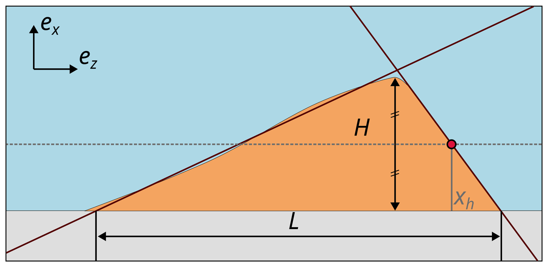
Figure D1 Schematic showing how the dune's characteristics are defined. The dune's position is tracked using the coordinate x_h corresponding to the abscissa of the mid-height of the downstream side of the dune. The dune's length is the base of the triangle formed by the lines approximating the downstream and upstream slopes and the rigid bed.

Table D1 Characteristics of the four meshes used in the numerical study of dune migration. Ranging from coarse mesh M0 to fine mesh M3. The domain length is 800 mm, and the domain height is 90 mm for all meshes. n_x and n_z are the number of cells in the x-direction and z-direction, respectively, and z₁ is the distance from the first cell center to the wall boundary.

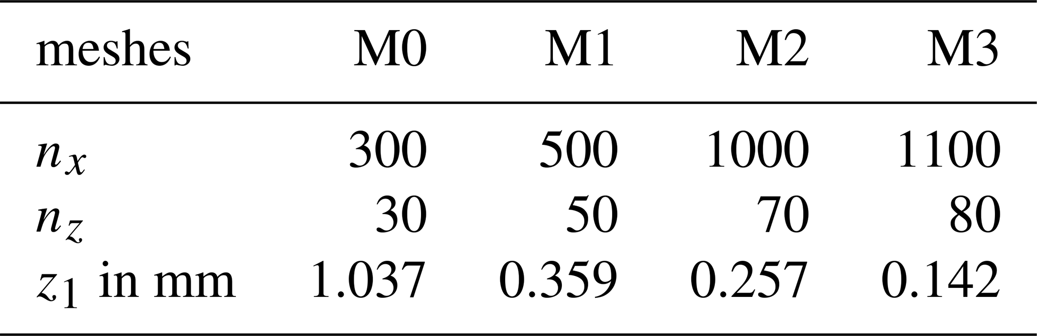
As stated in Sect. 5, the migration of the dune is affected by various parameters of the model. A first important parameter is the mesh resolution and, in particular, the near-bed resolution. A poor resolution leads to an underestimate of the bed shear stress. Table D1 summarizes the characteristics of four different meshes used in a sensitivity analysis.

The bed motion is deactivated to study the effect of mesh resolution on the bed shear stress without morphodynamics, and each simulation is run for 10 s in order to reach a stationary state. Figure D2 shows the stream-wise component of the bed shear stress obtained with the four meshes presented in Table D1.

The maximum friction velocity consistently occurs slightly upstream of the crest. Its position is sensitive to mesh resolution, shifting farther upstream as the mesh is refined. Poor mesh resolution leads to an underestimation of the maximum friction velocity near the dune crest, which can slow the migration process in morphodynamics simulations. Using a fine mesh also reveals additional flow features near the dune extremities. For instance, a small recirculation develops at the upstream foot of the dune, and the friction velocity decreases at the transition between the downstream slope and the flat bed.

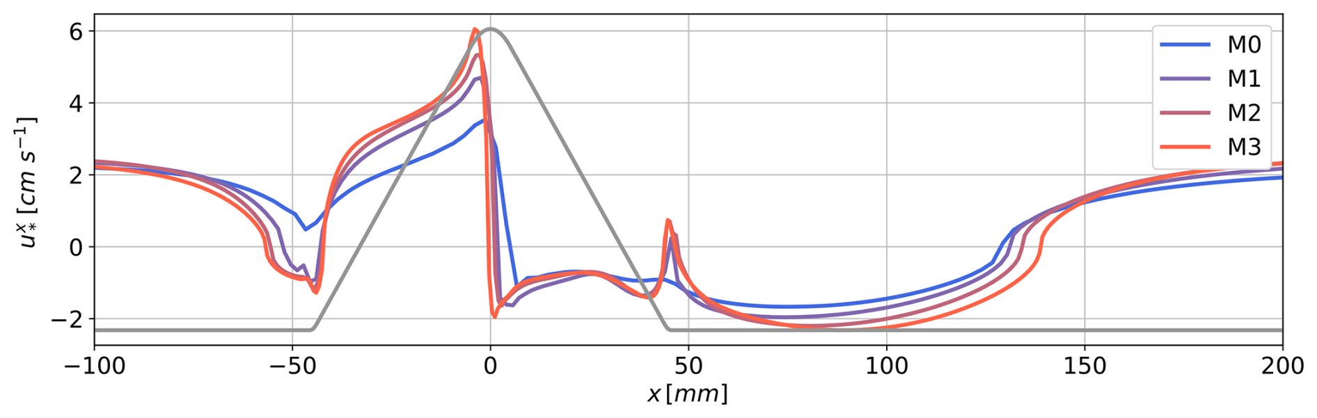
Figure D2 Comparison of the streamwise component of the friction velocity for four mesh resolutions (M0, M1, M2, and M3) in simulations of flow over the initial dune geometry without morphodynamic evolution.

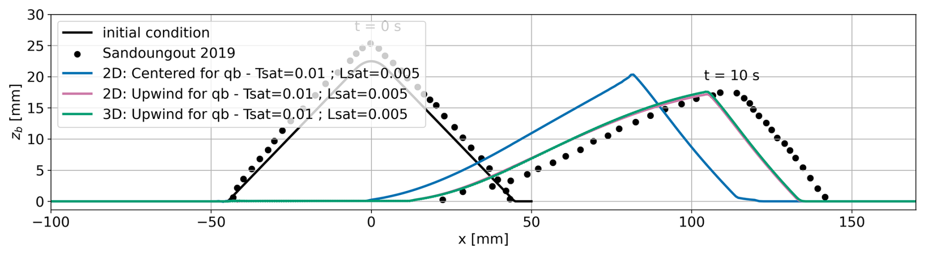
Figure D3 Bed elevation obtained with different advection schemes for the divergence of bedload flux in the Exner equation: Upwind and Linear (Centered) schemes, coupled with a second order Adams-Bashforth scheme for the time derivative. The saturation length value is fixed to L_sat=5 mm and the saturation time is fixed to T_sat=0.01 s.