Recognizing spatial geochemical anomaly patterns using deformable convolutional networks guided with geological knowledge

This study tackles the limited quantification of irregular spatial geochemical anomaly patterns and weak interpretability in deep learning models in geochemical anomaly recognition. We propose a hybrid approach that integrates geological knowledge (GK) into deformable convolutional networks (DCN), creating a model termed GK-DCN, with the aim of enhancing both the performance and transparency of geochemical anomaly recognition. This model introduces learnable parameters that allow the convolution kernel to adaptively adjust its shape according to the characteristics of its sampling position, enabling them to more accurately capture complex and irregular geochemical anomaly patterns caused by mineralization. To enhance geological consistency, ore-controlling faults are incorporated as geological knowledge constraint, guiding the network to prioritize spatial correlations between deposits and faults. Experimental results in southern Tianshan Au-Cu polymetallic ore district demonstrate that the GK-DCN, verified across multiple evaluation metrics, significantly enhances the accuracy and reliability of geochemical anomaly recognition, Besides, it produces more distinct spatial anomalous patterns and higher consistency with known mineral deposits by adaptively adjusting the receptive field. Visualization of the kernel offsets revealed the model's superior adaptive spatial sampling mechanism. Furthermore, feature significance heatmaps generated by Grad-CAM (Gradient-weighted Class Activation Mapping) highlighted the key features that the model focused during geochemical anomaly recognition. These visualizations significantly improve the interpretability and prove the effectiveness in capturing complex geochemical patterns. This work provides an effective intelligent method for spatial geochemical pattern recognition and offers a reference for interpretable deep learning in geochemical exploration through multi-angle visualization.

1 Introduction

Geo-anomalies, detected through various observational datasets such as geological, geochemical, geophysical, and remote sensing methods, play a vital role in identifying mineralization-related geological processes. Their significance lies in the fact that these anomalies reveal underlying causative features or events that are not directly observable (Cheng and Zhao, 2011). Hydrothermal mineralization is a systematic yet complex geological phenomenon, involving the migration of ore-bearing hydrothermal fluids, interactions between fluids and host rocks, mineral precipitation, and the eventual concentration of economic minerals (Pirajno, 2008). Since these processes result from the interplay of multiple geological factors operating across different spatial and temporal scales, the associated geo-anomalies display considerable complexity (Cheng, 2012). Analyzing their spatial distribution can significantly refine and advance geological understanding of numerous scientific questions. Geochemical anomalies associated with mineralization represent one of the most significant types of geo-anomalies for mineral exploration (Zuo et al., 2021). These anomalies often exhibit anisotropic spatial distributions that are controlled by ore-forming geological structures (e.g., strata, faults, and magmatic intrusions), which provide essential space, heat, fluid, and material conditions for mineralization (Pirajno, 2008). For example, hydrothermal mineralization frequently presents as linear-trending geochemical anomalies along fault zones, where fault systems act as pathways for the transport and deposition of ore-forming materials (Wang et al., 2013). Consequently, recognizing the spatial anisotropy of geochemical anomaly patterns is crucial for accurately identifying significant anomalies, thus can greatly enhance the success rate of mineral exploration (Cheng, 2012; Zuo, 2017; Xiao et al., 2018).

Long-term research and practice have demonstrated that integrating spatial structure through spatial autocorrelation analysis, spatial decomposition, moving window statistics, and spatially aware machine learning offers a more geologically realistic and robust framework for recognizing geochemical anomalies. Spatial autocorrelation analysis, using methods like local Moran's I, helps detect statistically significant spatial clusters-such as high-high clusters (indicating potential anomalies surrounded by other high values) and high-low clusters (representing isolated high values) (Yin et al., 2021). Spatial decomposition primarily employs the following methods: Kriging, Trend Surface Analysis and Multifractal Filtering. Kriging, allow for the estimation of values at unsampled locations, generating a spatially continuous model of the geochemical background. Anomalies are identified where measured values significantly exceed the Kriging predictions, indicated by large prediction errors (Jimenez-Espinosa et al., 1993). Additionally, incorporating directional variograms into Kriging methods, such as anisotropic ordinary Kriging, enables explicit accounting for directional trends and local heterogeneity in anomalies (Reis et al., 2003). Trend surface analysis involves fitting polynomial surfaces, using either global or local regression, to model regional trends. The residuals derived from this surface represent local deviations, which can serve to highlight anomalies against the broader regional pattern (Wang and Zuo, 2015). Multifractal filtering methods mainly include the Concentration-Area (C-A) model and the Spectrum-Area (S-A) model (Cheng et al., 1994, 2000). These methods plot element concentration against area and identify breaks in the observed power-law (scaling) behavior. These breakpoints are used to separate background populations from anomalous ones. This approach explicitly models the scale-dependent heterogeneity of spatial patterns and establishes thresholds based on deviations from fractal behavior across different scales (Cheng, 2012). Moving window statistics methods, such as local singularity analysis and the local gap statistic, calculate local statistics (e.g., mean, median, standard deviation) within a defined spatial window (Cheng, 2007; Wang and Zuo, 2016). Values that significantly exceed the local background within their respective window are identified as geochemical anomalies. This technique effectively captures local spatial context and non-stationarity, although the choice of window size is a critical and subjective step. To account for anisotropy, these methods are further modified by incorporating elliptical or directionally weighted windows (Xiao et al., 2018, 2020; Wang et al., 2018). The final category for analyzing geochemical spatial patterns is spatially aware machine learning. This approach primarily includes two types: models that integrate spatial features or components (Cheng et al., 2011; Wang et al., 2015), and models with inherent capabilities to capture spatial structures (LeCun and Bengio, 1998). In the first type, spatial characteristics are incorporated into traditional statistical methods through distance-based kernels or spatial weighting schemes to address geographic heterogeneity and non-stationarity. Commonly used spatially weighted machine learning techniques for identifying geochemical anomaly patterns include geographically weighted regression (GWR) (Wang et al., 2015; Tian et al., 2018), spatially weighted principal component analysis (SWPCA) (Cheng et al., 2011; Xiao et al., 2012), density-based spatial clustering of applications with noise (DBSCAN) (Zhang et al., 2019; Hajihosseinlou et al., 2024), and geographical random forest (GRF) (Soltani et al., 2024). The second type involves machine learning architectures specifically designed to handle spatial data, such as convolutional neural networks (CNN) (LeCun and Bengio, 1998) and graph neural networks (GNN) (Scarselli et al., 2008). In the application of deep learning in spatial geochemical anomaly recognition, various advanced deep learning models have been proposed, which mainly involves: graph-based model, Transformer, spatial-spectrum dual-branch model and informed model (Xu et al., 2025a). These methods are capable of characterizing complex spatial relationships effectively in geochemical survey data (Zhang et al., 2021; Xu et al., 2023, 2024b, 2025a; Liang et al., 2025; Chen and Zuo, 2025); modelling both spatial and spectrum characteristics simultaneously while accounting for inherent heterogeneity of the data (Zuo and Xu, 2024; Xu and Zuo, 2025; Xu et al., 2025b); and considering geological knowledge to enhance its interpretability (Xiong et al., 2022; Luo et al., 2023; Zuo et al., 2024, 2025; Xu et al., 2025a). CNN and GNN are mostly adopted as the basis framework in these models. CNN learns local spatial features and mineralization-related patterns through convolutional and pooling operations (Chen et al., 2019; Zhang et al., 2021; Huang et al., 2022; Yang et al., 2023). However, a key limitation is their reliance on fixed, regular convolution kernels (e.g., 3×3 grids), which restricts their ability to adequately model the anisotropic nature of geochemical patterns (Dai et al., 2017). In contrast, GNN directly represents non-Euclidean spatial relationships using nodes (e.g., sample points with geochemical attributes) and edges (encoding spatial proximity or geological links), allowing anomaly recognition based on complex neighborhood interactions (Xu et al., 2023, 2024b, 2025a; Liang et al., 2025; Chen and Zuo, 2025). Nevertheless, GNN requires high-quality data and substantial domain knowledge to define meaningful graph structures. In particular, defining appropriate edges based on spatial distance or geological similarity is crucial yet challenging. Improper edge definitions may introduce noise, mask genuine anomalies, and ultimately impair model performance (Gong and Cheng, 2019; Zhou et al., 2020).

Deformable Convolutional Networks (DCN) address a fundamental constraint of traditional CNN: the fixed geometric structure of their convolution kernels (Dai et al., 2017). By introducing learnable spatial offsets for each sampling point in the kernel, DCN adaptively adjust the sampling locations, effectively warping the kernel's receptive field to align with irregular and complex patterns (Dai et al., 2017; Zhu et al., 2018). This flexibility allows the kernel to conform non-rigid and deformed structures, enabling more precise feature extraction from key regions of irregular shapes (Dai et al., 2017; Zhu et al., 2019). As a result, DCN exhibit greater robustness to geometric variations such as changes in orientation, scale, or deformation, maintaining consistent feature representation across diverse pattern states. These capabilities make DCN valuable in tasks involving irregular spatial structures. By offering essential spatial adaptability, DCN provide a powerful tool for analyzing the complex and often messy geometries encountered in various domains, which involve irregular seismic data interpolation (Zhao et al., 2023; Luo et al., 2024; Sun et al., 2024), earthquake crack detection (Yu et al., 2022), flood boundary detection (Yu et al., 2023), surface wave suppression (Gao et al., 2024), underwater image enhancement (Tian et al., 2023), atmospheric forecasting (Nielsen et al., 2022), precipitation forecasting (Xu et al., 2024a), morphological characteristics of clouds modelling (Liu et al., 2021), images denoising (Guan et al., 2022; Liu et al., 2024), hyperspectral image classification (Zhu et al., 2018; Zhao et al., 2021), identification of anomalous deformation areas (Zhang et al., 2022), hyperspectral anomaly detection (Wu et al., 2023), and soil moisture monitoring (Na et al., 2025). By capturing spatial deformations, DCN offer a transformative approach for extracting meaningful metrics from the inherent irregularity of geoscientific data.

In this study, we utilize a DCN as the foundational model for recognizing and extracting complex anisotropic geochemical spatial patterns. Just as purely data-driven deep learning methods such as CNN face interpretability issues, so does the DCN, whose function is regarded as complex “black box”. While they achieve high prediction accuracy, understanding why they make a specific prediction, which features in the input data were decisive, or how their learned representations map to established geological concepts is extremely difficult (Gilpin et al., 2018; Rudin, 2019). Current approaches to enhance the interpretability of deep learning models primarily operate at three stages: model input, model construction, and model output (Zuo et al., 2024). At the model input stage, interpretability is enhanced through metallogenic models, feature engineering, and geologically constrained data augmentation methods (Zuo et al., 2024). At the model construction stage, key ore-controlling factors are integrated into the hidden layers, while the spatial coupling relationship between known mineral deposit locations and these factors is incorporated into the loss function (Xiong et al., 2022; Luo et al., 2023; Zuo et al., 2025). At the model output stage, visualization techniques are employed to examine the outputs of each hidden layer, providing insight into the extraction and integration processes of prospecting information. Meanwhile, attribution techniques are applied to assess the importance of input variables, helping to quantify their contributions to the formation of mineral deposits (Luo et al., 2023; Xu et al., 2025a). In this study, we enhance the interpretability of the DCN at both the model construction and output stages. During model construction, a governing equation representing the spatial correlation between known mineral deposits and ore-controlling factors is embedded into the loss function (Xiong et al., 2022; Zuo et al., 2024). This approach introduces conceptual models and expert knowledge into the training process, ensuring that the model's results are consistent with established geological principles (Zuo et al., 2024). At the model output stage, we utilize class activation mapping (CAM) (Jung and Oh, 2021) and its variant, Grad-CAM (Selvaraju et al., 2016), to visualize the regions within the input data that most influence the model's predictions. CAM visually identifies the most discriminative regions in an input image responsible for a specific class prediction of CNN and DCN. It leverages the weights of the final fully connected layer to compute a weighted sum of the activation maps from the last convolutional layer, thus can transform CNN and DCN from a “black box” into a more transparent model by generating a heatmap (class activation map). Besides, the learned offsets are also visualized to reveal how DCN dynamically adapts sampling locations, enhancing the understanding of model behavior for spatial pattern quantification. Ultimately, the constructed model was applied to the study area of the southern Tianshan Au-Cu polymetallic ore district to verify its effectiveness and interpretability in identifying geochemical anomalies.

2 Geological setting and Datasets

2.1 Geological setting

The South Tianshan Metallogenic Belt, extending across Central Asia from Uzbekistan through Tajikistan, Kyrgyzstan, and into western China (Xinjiang), is one of the world's most significant gold and copper provinces (Fig. 1). Its formation is intrinsically linked to the protracted and complex tectonic history of the Central Asian Orogenic Belt, specifically the final closure of the Paleo-Asian Ocean (Gao et al., 2009; Han et al., 2011). The regional geology is dominated by the collage of multiple terranes, including Precambrian continental blocks, early Paleozoic oceanic crust fragments, and island arcs, which were accreted and subsequently deformed during the Late Paleozoic collision between the Tarim Craton to the south and the Kazakhstan-Yili Block to the north (Gao et al., 2009). This continental collision, culminating in the Late Carboniferous to Early Permian, created a major suture zone characterized by extensive thrusting, folding, and large-scale strike-slip fault systems. These structures provided crucial conduits for subsequent fluid migration and mineralization.

The primary mineralization events are temporally and genetically associated with this collisional orogeny and the post-collisional extensional phase. Two major mineralization styles prevail: (1) Orogenic gold deposits, often hosted in shear zones within Neoproterozoic to Paleozoic metamorphic rocks (e.g., the giant Muruntau deposit in Uzbekistan). These deposits formed from metamorphic fluids released during devolatilization of subducted slabs or thickened crust. (2) Copper-gold skarn and porphyry-style mineralization, frequently associated with Late Carboniferous to Permian post-collisional I-type granitoids intruding carbonate-rich sequences. These intrusions provided the heat and magmatic fluids responsible for widespread hydrothermal alteration and metal deposition. The conjunction of fertile source rocks (often black shales), ideal structural traps (fault jogs, shear zones, lithological contacts), and the timing of magmatism relative to tectonic stress changes created the perfect conditions for the formation of world-class gold and copper deposits. The Chinese segment of the South Tianshan, such as the Sawayaerdun gold belt, continues this metallogenic trend, hosting numerous deposits with similar genetic models (Chen et al., 2012; Goldfarb et al., 2014; Seltmann et al., 2014).

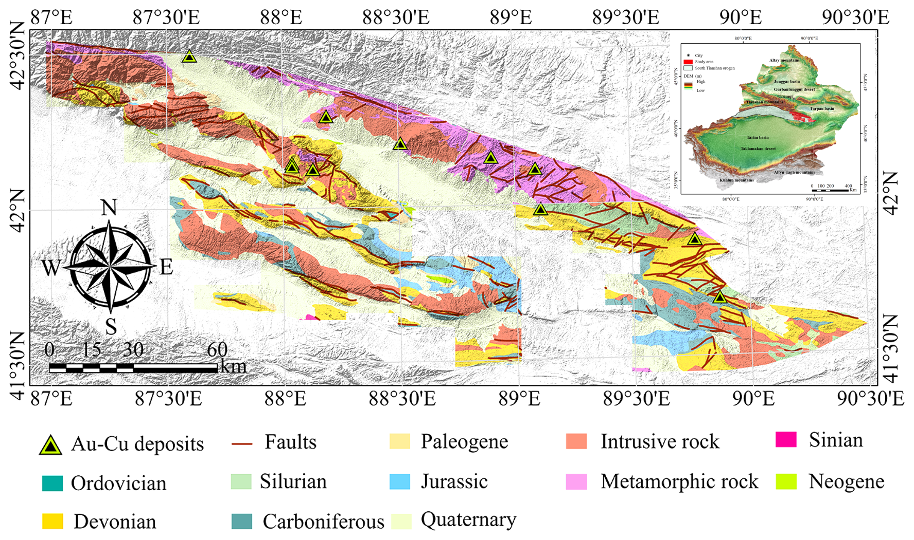
Figure 1 Simplified geological map of the Southern Tianshan showing the main tectonic units and Au-Cu deposits (modified from Xue et al., 2014; Zhao et al., 2020).

2.2 Datasets

The 1:200 000 scale geochemical samples in this study area were sourced from the Chinese National Geochemical Mapping Project (Xie et al., 1997; Wang et al., 2007). The standard sampling density was 1–2 samples per square kilometer, with every 4 km² constituting one analytical unit. Sampling density was appropriately reduced in areas where fieldwork was difficult to conduct (1 sample per 20–50 km²). Multiple sub-samples were collected within a certain range (20–50 m) around the sampling point and combined into a single composite sample. The sample was sieved through a 60-mesh stainless steel screen, with the final sample weight exceeding 200 g. A total of 32 elements and 7 oxides were analyzed: Bi, Cu, P, La, Li, Ag, Sn, Au, Mo, Th, U, Y, W, Sb, Hg, Mn, Cr, Sr, Nb, Pb, Ni, Ti, Cd, Co, Ba, Be, V, Zn, B, As, Zr, F, as well as Fe₂O₃, K₂O, CaO, MgO, Na₂O, Al₂O₃, and SiO₂. The detection limits and analytical methods for each element are listed in Table 1.

Table 1 Elements, analytical methods, and detection limits from the Chinese national geochemical mapping project.

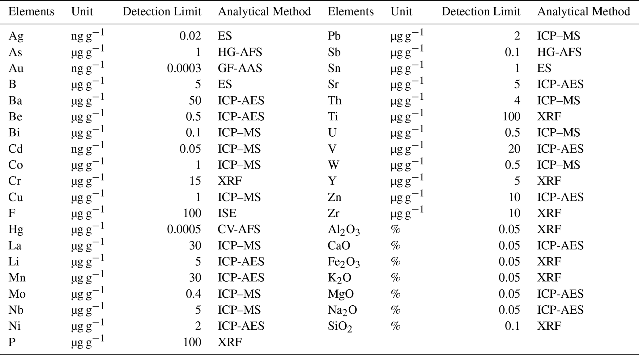
Note: XRF: X-ray fluorescence spectrometry; ICP-AES: Inductively coupled plasma-atomic emission spectrometry; ICP–MS: Inductively coupled plasma–mass spectrometry; ES: Emission spectrometry; HG-AFS: Hydride generation atomic fluorescence spectrometry; GF-AAS: Graphite furnace atomic absorption spectrometry; CV-AFS: Cold vapor atomic fluorescence spectroscopy; ISE: Ion selective electrode.

3 Methods

3.1 Deformable convolutional networks (DCN)

Deformable convolution networks (Dai et al., 2017; Zhu et al., 2019), enables adaptive adjustment of the receptive field positions by incorporating learnable offset parameters for each sampling point within the convolutional kernel. Figure 2 illustrates the distinction between the sampling points of standard convolution and those of deformable convolution. This approach overcomes the limitations imposed by a fixed grid structure, thereby facilitating more flexible and precise extraction of image features exhibiting complex geometric deformations.

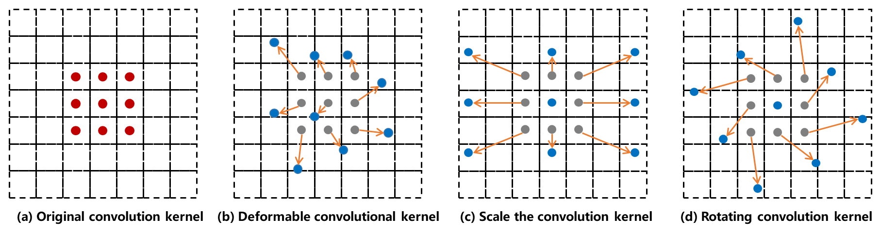
Figure 2 Illustration of the sampling locations in 3×3 standard and deformable convolutions. (a) Regular sampling grid of standard convolution; (b–d) deformed sampling locations of deformable convolution with augmented offsets. The red areas are the sampling locations in 3×3 standard convolution. The grey areas and the blue areas are the initial sampling locations and final sampling locations of the deformable convolution, respectively. The yellow arrow points from the initial sampling location to the corresponding final sampling location.

The computation involved in deformable convolution remains a form of two-dimensional convolution, with an emphasis on spatial interactions across all channels. The fundamental aspect of this method lies in learning the offsets of sampling points via a parallel branch network, allowing the convolutional kernel to dynamically adjust its sampling locations based on the content of the input feature map. This mechanism directs convolutional operations to concentrate on regions of interest, substantially enhancing the network's capacity to represent features associated with geometric transformations.

In this study, a standard 3×3 two-dimensional convolutional kernel, denoted as R, is employed as an illustrative example.

$$\begin{array}{}\text{(1)}& R=\left(-\mathrm{1},-\mathrm{1}\right),\left(-\mathrm{1},\mathrm{0}\right),\mathrm{\cdots },\left(\mathrm{0},\mathrm{1}\right)\left(\mathrm{1},\mathrm{1}\right)\end{array}$$

In conventional convolutional kernels, the weight matrix is denoted by w, the input feature map by x, and p_n represents any pixel within the convolutional window R. For each output position p₀ in the feature map, the convolution operation can be mathematically expressed as follows:

$$\begin{array}{}\text{(2)}& y\left(p_{\mathrm{0}}\right)=\sum _{p_n\in R}w\left(p_n\right)x\left(p_{\mathrm{0}}+p_n\right)\end{array}$$

In the context of deformable convolution, the introduction of an offset $\mathrm{\Delta }{p}_n\mathrm{\Delta }{p}_n\mid n=\mathrm{1},\mathrm{\cdots },NN=\mathrm{|}R\mathrm{|}$ modifies the original formulation, transforming it into:

$$\begin{array}{}\text{(3)}& y\left(p_{\mathrm{0}}\right)=\sum _{p_n\in R}w\left(p_n\right)\times \left(p_{\mathrm{0}}+p_n+\mathrm{\Delta }{p}_n\right)\end{array}$$

This adjustment results in sampling points that are spatially shifted, with the offset positions denoted as p_n+Δp_n. Since the offset Δp_n generally assumes non-integer values, the computation of the convolution must be performed using bilinear interpolation, as described by:

$$\begin{array}{}\text{(4)}& x\left(p\right)=\sum G\left(q,p\right)x\left(q\right)\end{array}$$

The value at any position p is thus a function of $p=p_{\mathrm{0}}+p_n+\mathrm{\Delta }{p}_n$ and is computed over all spatial locations q within the input feature map x by employing the bilinear interpolation kernel $G\left(\cdot ,\cdot \right)$. Notably, the two-dimensional interpolation kernel is separable and can be decomposed into the product of two one-dimensional kernels, which serves to optimize computational efficiency:

$$\begin{array}{}\text{(5)}& G\left(q,p\right)=g\left(q_x,p_x\right)g\left(q_y,p_y\right)\end{array}$$

where $g(a,b)=max(\mathrm{0},\mathrm{1}-\mathrm{|}a-b\mathrm{|})$.

Figure 3 delineates the detailed implementation procedure of deformable convolutional layers. Initially, the learned offset vectors are applied to the fixed sampling grid of the input feature map, enabling adaptive adjustment of each sampling point's position. Subsequently, bilinear interpolation is utilized to estimate feature values at the offset, non-integer coordinate locations, thereby ensuring that the sampled feature distribution effectively concentrates on the target region. Figure 4 provides a comparative visualization between standard convolution and deformable convolution with respect to their receptive fields for geochemical pattern recognition. By incorporating offsets, the receptive field in deformable convolution transcends the constraints imposed by the fixed, regular grid of standard convolution. This flexibility allows the receptive field to adaptively assume irregular spatial configurations that better correspond to the actual geometric structure of the target object, thereby substantially enhancing the accuracy of feature extraction.

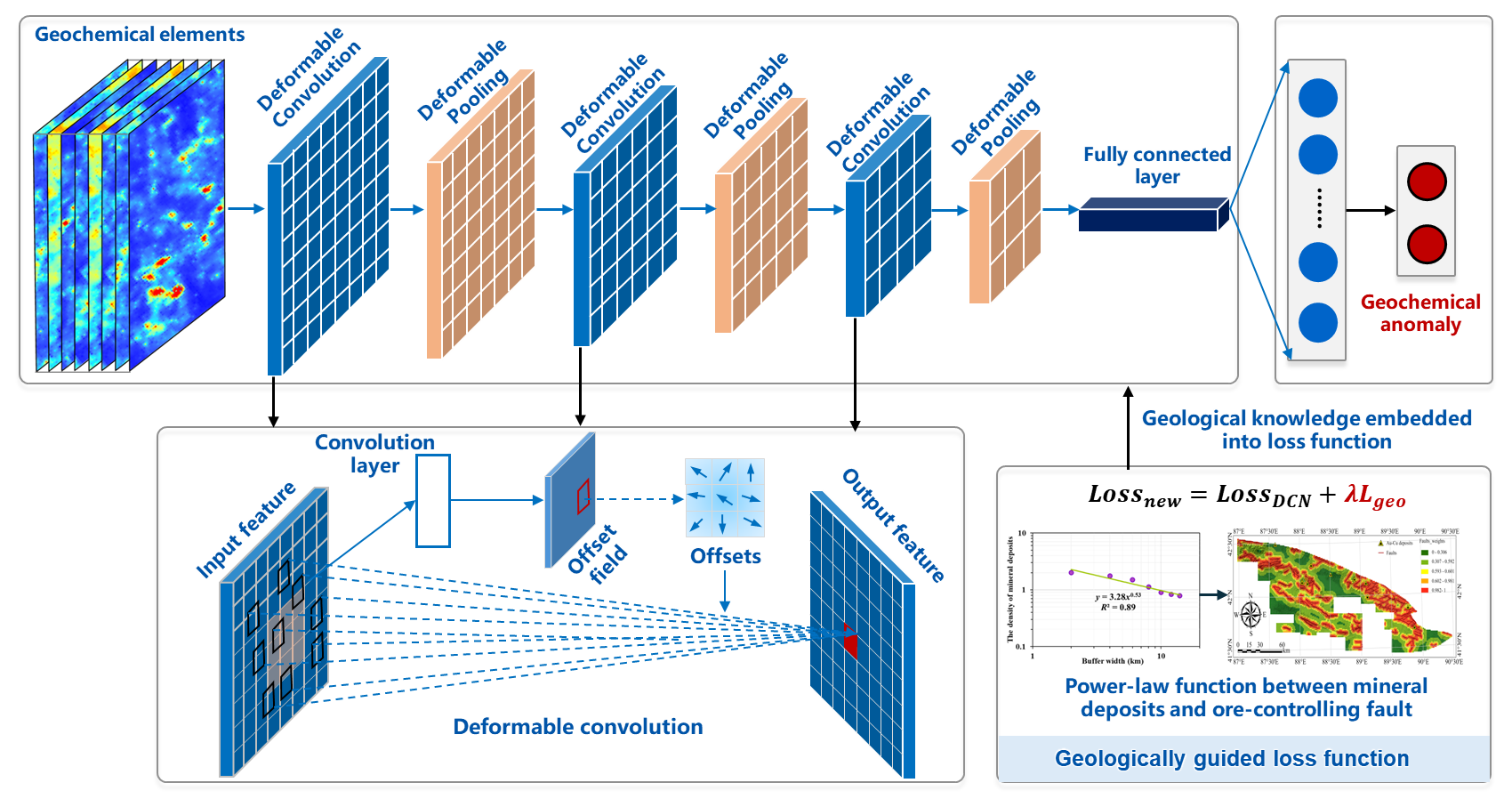
Figure 3 The framework of proposed geological knowledge guided deformable convolution networks.

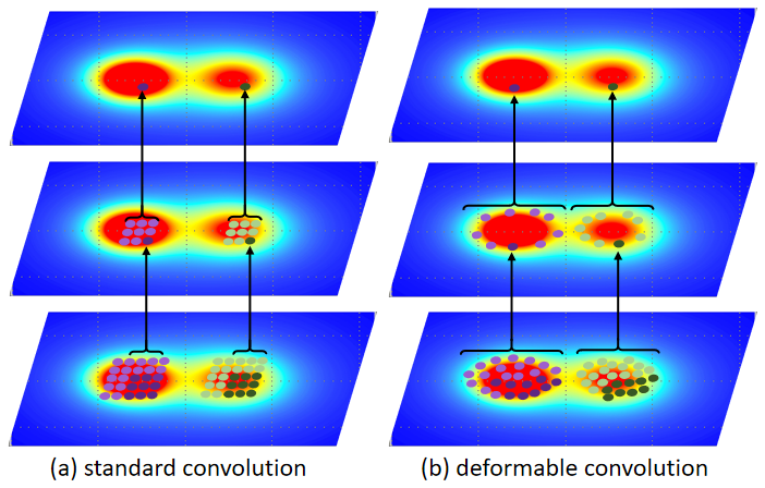
Figure 4 Illustration of the sampling locations for (a) normal convolution and (b) deformable convolution. Maps showing irregular geochemical patterns. It is observed that deformable convolutions can adaptively extracts the features of the input by adjusting its shape according to the actual patterns by shifting the convolutional kernel, but normal convolutions only describe the fixed receptive field.

3.2 Geologically-constrained DCN

This study introduces soft constraint on deformable convolutional networks to enhance geochemical anomaly detection by incorporating geological prior knowledge. In typical geochemical anomaly recognition tasks, deformable convolutional neural networks optimize their parameters by minimizing the cross-entropy loss, which measures the divergence between predicted and true label distributions. To improve this optimization process, the present work augments the loss function with an additional penalty term derived from established geological principles, thereby guiding the model to learn feature representations that better conform to geological laws (Semenov et al., 2019).

The conventional loss function L_DCN, is defined as follows:

$$\begin{array}{}\text{(6)}& L_{\mathrm{DCN}}\left(p,\widehat{p}\right)=-\sum _{x}p\left(x\right)\log \widehat{p}\left(x\right)\end{array}$$

where p(x) and $\widehat{p}\left(x\right)$ denote the true and predicted distributions, respectively. Building upon this, a novel penalty term grounded in geological knowledge is formulated and integrated into the loss function. Following the approach proposed by Zuo (2016) for penalty term construction, the relationship between the distance control factor and the spatial distribution of mineral deposits is modeled by a power-law function w, expressed as:

$$\begin{array}{}\text{(7)}& w={\displaystyle \frac{m}{m_{max}}}={\displaystyle \frac{N{d}^k}{m_{max}}}\end{array}$$

where N is a constant, d represents the distance between the control factor and the mineral deposit, m denotes the density of mineral deposits at distance d, and k corresponds to the line fitting parameters relating log ^m and log ^d. w serves as a control equation embedding prior geological knowledge to characterize the spatial coupling between known mineral occurrences and their controlling factors. As the DCN progressively learns the spatial distribution patterns between mineral deposits and their surrounding grid units, it becomes essential to extract spatial structural features encapsulated by the weight function w and incorporate them into the training process. Consequently, a geology-informed penalty term L_geology is constructed, formulated as:

$$\begin{array}{}\text{(8)}& L_{\mathrm{geology}}=\mathrm{|}\mathrm{|}{f}_{\mathrm{softmax}}\left(\widehat{p}\right(x\left)\right)-f_{\mathrm{sigmoid}}\left(\sum _{i=\mathrm{1}}^{n}a{w}_i+b\right)\mathrm{|}{\mathrm{|}}_{\mathrm{2}},\end{array}$$

where a and b are trainable parameters within the combined kernel used for feature aggregation, with a representing weights and b denoting bias terms; n is the number of feature maps. The aggregated features undergo normalization via the function f_sigmod, and the network output is subsequently transformed into mineral potential prediction values through the mapping function f_softmax.

Finally, a comprehensive loss function L_total is developed for the deformable convolutional network, integrating prior geological knowledge, and is expressed as:

$$\begin{array}{}\text{(9)}& L_{\mathrm{total}}=L_{\mathrm{DCN}}+\mathit{\lambda }{L}_{\mathrm{geology}}.\end{array}$$

This formulation effectively constrains the model to produce predictions that are consistent with both data-driven learning and established geological understanding (Fig. 3). The regularization parameter λ has a crucial effect on deep learning training and prediction performance owing to its role in controlling the balance between the data loss and geological constraint loss. A larger value of λ leads to a higher training loss at the expense of the geological penalty term, and vice versa. Specifically, a larger value of λ gives the deep learning model a better chance of learning geological-related patterns, while a smaller value of λ gives the deep learning model a better chance of learning general patterns from data. Thus, the regularization parameter λ should be carefully chosen (Xiong et al., 2022). To balance the data loss and the geological constraint loss, the parameter is set to 1.

3.3 Gradient-weighted Class Activation Mapping

To improve the interpretability and discriminative localization capabilities of deformable convolutional neural networks, the integration of class activation mapping (CAM) techniques is employed. The conventional CAM approach leverages the weights from the global average pooling (GAP) layer and the final classification layer to visualize the discriminative regions utilized by the CNN during classification. By projecting the output layer's weights back onto the convolutional feature maps, the relative importance of different image regions is identified.

Initially, it is necessary to remove all fully connected layers following the last convolutional block, as CAM requires a fully convolutional architecture to maintain spatial information up to the final layer. A GAP layer is introduced subsequently to the last deformable convolutional layer to substitute the fully connected layers (Jung and Oh, 2021). The function of this GAP layer is to compute the spatial average value F^k of each feature map in the final convolutional layer, which can be mathematically expressed as:

$$\begin{array}{}\text{(10)}& F_k={\displaystyle \frac{\mathrm{1}}{X\cdot Y}}\sum _{x=\mathrm{1}}^X\sum _{y=\mathrm{1}}^Y{f}_k\left(x,y\right),\end{array}$$

where f_k(x,y) denotes the activation at spatial location (x,y) in the kth channel of the feature map output by the last deformable convolutional layer, and X and Y represent the width and height of the feature map, respectively.

Following the GAP layer, a single fully connected layer with a softmax activation function is appended. For a given class c, this layer assigns a weight $w_k^c$ to each averaged feature map value f_k(x,y). The linear classification logit score S_c for class c is then computed as:

$$\begin{array}{}\text{(11)}& S_{\mathrm{c}}=\sum _k{w}_k^c{F}_k={\displaystyle \frac{\mathrm{1}}{X\cdot Y}}\sum _{x,y}\sum _k{w}_k^c{f}_k\left(x,y\right),\end{array}$$

where S_c is a scalar representing the classification score. To generate the class activation map, the weights $w_k^c$ are multiplied element-wise with the corresponding feature maps F^k and summed across all channels:

$$\begin{array}{}\text{(12)}& M_c\left(x,y\right)=\sum _k{w}_k^c{f}_k\left(x,y\right).\end{array}$$

This operation preserves spatial information along the width and height dimensions. Subsequently, bilinear interpolation is applied to upsample the matrix M_c to the original input image size, thereby producing the complete CAM visualization.

In summary, each feature map channel corresponds to a specific class of visual features extracted by a convolutional kernel from the input image. The weights $w_k^c$ implicitly indicate the significance of these features for the classification of category c, reflecting the degree of attention that the model allocates to each feature with respect to that class.

However, CAM technique necessitates the substitution of the fully connected layer with a GAP layer and is limited to analyse only the final convolutional layer. To overcome these constraints, we adopted the Gradient-weighted CAM (Grad-CAM) approach, which derives the requisite weights indirectly through gradient computations rather than depending on the GAP layer and softmax activation (Selvaraju et al., 2016). Consequently, it enables the generation of class-specific activation heatmaps for convolutional layers situated at various depths within the network.

The Grad-CAM algorithm computes the gradient of the target score, which typically correspond to the class of interest, with respect to the feature maps of a selected convolutional layer. From these gradients, the importance weight ${\mathit{\alpha }}_k^c$ for each channel k is obtained, as expressed by the following equation:

$$\begin{array}{}\text{(13)}& {\mathit{\alpha }}_k^c={\displaystyle \frac{\mathrm{1}}{Z}}\sum _{i=\mathrm{1}}^u\sum _{j=\mathrm{1}}^v{\displaystyle \frac{\partial y^c}{\partial A_{ij}^k}},\end{array}$$

where c denotes the target class, ${\mathit{\alpha }}_k^c$ represents the weight of the kth channel for class c, and y^c is the linear classification logit score for class c. The partial derivative $\frac{\partial y^c}{\partial A_{ij}^k}$ corresponds to the sensitivity of the output score y^c with respect to the activation at spatial location (i,j) in the kth feature map. u and v indicate the width and height of the feature map, respectively.

Mathematically, the weight ${\mathit{\alpha }}_k^c$ serves a role analogous to the weight $w_k^c$ in the original CAM formulation. By linearly combining these weights with the corresponding feature maps, the class activation map M_c can be computed as follows:

$$\begin{array}{}\text{(14)}& L_{\text{Grad-CAM}}^c=\mathrm{ReLU}\left(\sum _k{\mathit{\alpha }}_k^c{A}^k\right).\end{array}$$

The application of the ReLU function ensures that only features exerting a positive influence on the class c are retained. Finally, the resulting heatmap “M_c” is upsampled to match the input image dimensions using bilinear interpolation, thereby facilitating effective visualization of the class-discriminative regions (Fig. 5).

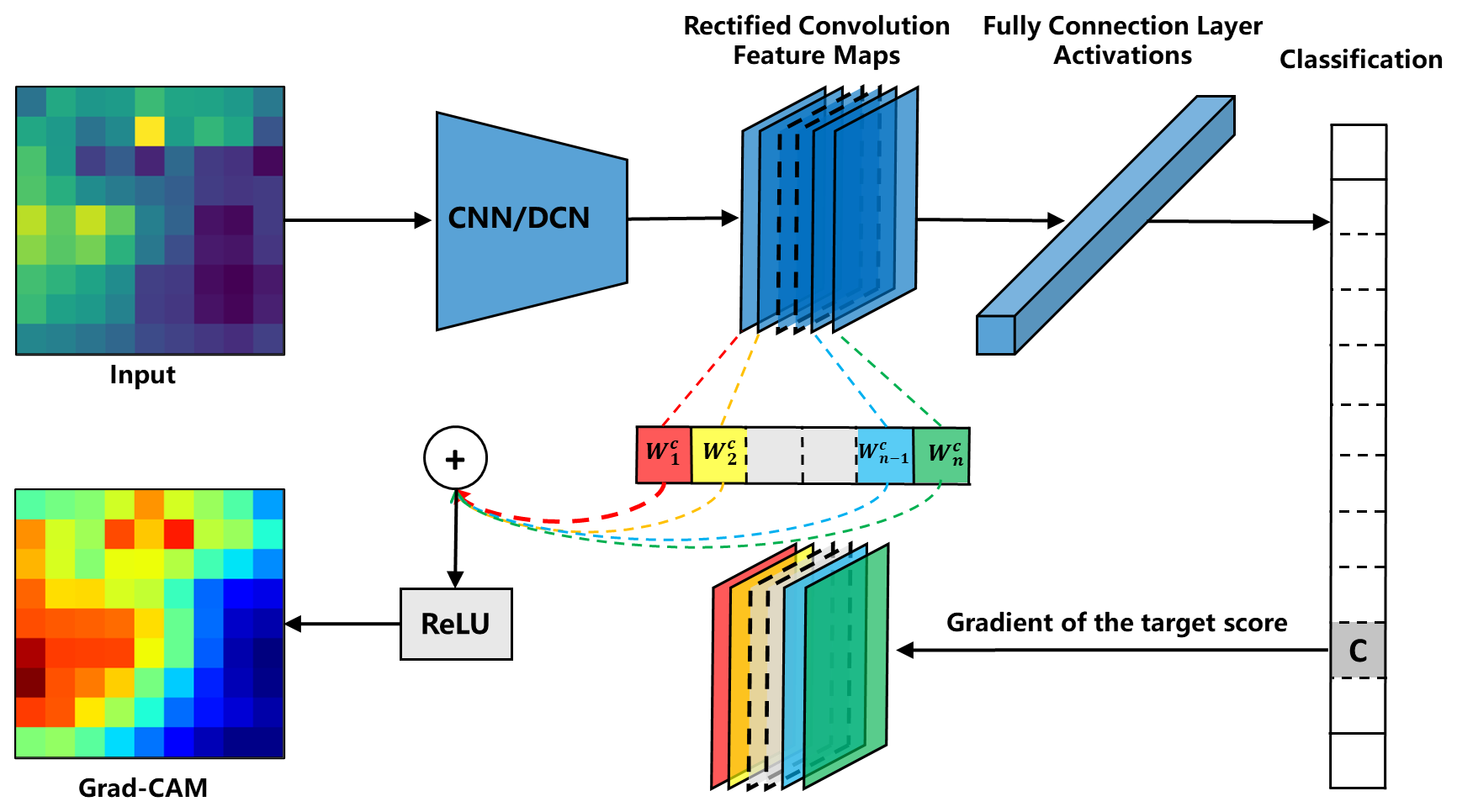
Figure 5 The workflow diagram for obtaining Grad-CAM within convolution neural network and deformable convolution networks.

4 Results and Discussions

The process begins by preprocessing the geochemical data. Each of the 39 elements is interpolated onto a 1 km × 1 km grid using Kriging interpolation. Small cubes are then cropped from this 3D grid and fed into a GK-DCN for feature extraction and anomaly recognition. As a supervised algorithm, the GK-DCN requires a dataset labelled with known anomalies (positive samples) and background (negative samples). Geochemical anomalies that deviate from regional patterns are key indicators of mineral deposits (Cheng, 2012). To model these anomalies, favorable areas were defined as 3×3 grid blocks centered on known Au-Cu deposits. From each central grid, a 9×9 cell patch was extracted, generating 84 positive samples representing mineralized areas. Negative samples were selected according to the following criteria (Carranza et al., 2008; Nykänen et al., 2015): (i) random non-deposit locations should be distant from known mineral deposit positions and favourable ore-controlling factors (e.g., faults); (ii) the number of selected non-deposit sites should match the number of known mineral deposit sites. The similar strategy was used for negative sample augmentation generating 84 patches. The dataset was split 8:2 for training and validation, resulting in a final input training data cube of dimensions $\mathrm{134}\times \mathrm{9}\times \mathrm{9}\times \mathrm{39}$ (67 patches per class).

4.1 Recognizing geochemical anomalies by GK-DCN

DCN and CNN exhibit significant differences in the extraction of geochemical anomalies. By introducing deformable convolution modules, DCN gains the ability to adaptively adjust the shape and size of receptive fields. Through the incorporation of learnable offset parameters, the convolutional kernels of DCN can dynamically deform based on the characteristics of the input data, learning the complex spatial distribution and structural features of geochemical elements. This allows the model to actively focus on the spatial anisotropy of geochemical anomalies, effectively capturing irregular anomaly patterns controlled by geological factors such as faults. The extracted anomaly boundaries show higher consistency with known ore-forming geological bodies and exhibit stronger spatial continuity (Fig. 6a). In contrast, CNN is constrained by its fixed geometric structure, leading to insufficient responsiveness to irregular boundaries. Its extraction results tend to be overly smooth, with significant loss of anomaly information (Fig. 6b). Comparative results demonstrate that DCN holds clear advantages in improving the spatial positioning accuracy of anomalies and their relevance to geological factors, providing more reliable geochemical indicators for mineral exploration. In summary, DCN significantly enhances the ability to represent the nonlinear and anisotropic characteristics of geochemical spatial distributions through its adaptive mechanism.

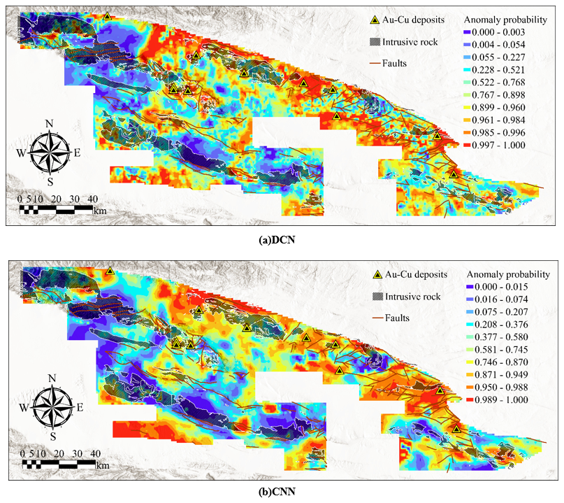
Figure 6 Geochemical anomalies associated with mineralization obtained by (a) DCN and (b) CNN.

Reflecting the geological setting where faults provided fluid pathways and deposition sites for Au-Cu mineralization, the quantified spatial relationship between ore-controlling faults and known deposits (Fig. 7) was incorporated into the DCN and CNN's loss function (Fig. 3). A non-linear controlling function between prospectivity density ρ and d was fitted: $\mathit{\rho }=\mathrm{3.28}{d}^{-\mathrm{0.53}}$. The d was the distance, and ρ was normalized for building a geologically constrained loss term. By incorporating geological constraints constructed from prior knowledge of fault-related mineralization to guide the training of both DCN and CNN, thus generating the GK-DCN and GK-CNN models. These models not only thoroughly learn the spatial distribution patterns and combinatorial relationships of geochemical elements but also strengthen their understanding of the geological background. This effectively suppresses background and noise interference unrelated to mineralization. The results show that compared to traditional methods, the anomalies extracted by the geologically constrained models exhibit higher spatial structural consistency with known mineralized fault structures, and the anomaly concentration centers are more prominent (Fig. 8). This approach significantly reduces the multiplicity of solutions in anomaly recognition and enhances the reliability and geological interpretability of the anomaly results.

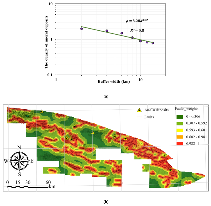
Figure 7 (a) Log–log plots between the density of mineral deposits ρ and the distance from faults. (b) Density value for faults in the case area.

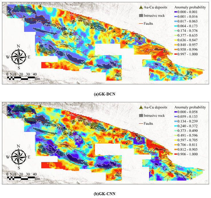
Figure 8 Geochemical anomalies associated with mineralization obtained by (a) GK-DCN and (b) GK-CNN.

To compare the feature extraction capabilities of CNN and DCN in the identification of geochemical anomalies, this study visualizes the offsets and employs Grad-CAM technology to visualize the spatial features learned by both types of models. These features are compared with the geochemical patterns, which are obtained by integrating multiple geochemical variables via Robust Principal Component Analysis (RPCA). PC1 vs. PC2 plots for the 39 elements (Fig. 9a) reveal two distinct compositional assemblages. The assemblage characterized by positive loadings of PC2 (Au, Cu, As, Hg, Bi, Mo, W, Co, Pb, Zn and Ni) (Fig. 9a) corresponds to Au–Cu mineralization in the region. The spatial distribution of PC2 scores (Fig. 9b) shows that high values, associated with this mineralization-related assemblage, correlate with areas of Au–Cu mineralization.

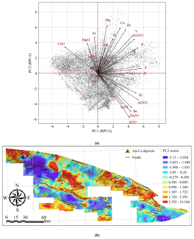
Figure 9 (a) Biplots of the PC1 and PC2 obtained by the RPCA methods, (b) Map showing the spatial distribution of the PC2 score related to mineralization.

As mentioned above, offsets are the core idea of deformable convolution. By introducing a parallel “offset prediction” structure, the network learns the shape and size of the receptive field on its own. For each sampling point of standard convolution, the network additionally learns two values (Δx, Δy), representing its offsets in the x and y directions. Thus, the actual sampling positions are no longer regular grid points but new positions formed by the original locations plus the predicted offsets. These new positions may distribute along the actual contours of the target object, thereby capture more precise features. Figure 10 illustrates the geochemical patterns corresponding to ten mineral deposits clipped from PC2 score maps, as well as the offsets direction and magnitude learned by the DCN for ten irregular spatial patterns. For irregular spatial patterns, deformable convolution adjusts the sampling positions of the convolution kernel through offsets. For each position of the convolution kernel, the deformable network adds their corresponding offsets to the original grid points, resulting in new sampling positions that pull the originally regular sampling points to more effective locations. The arrows pointing from the original grid points to the new sampling points represent the direction and magnitude of the offsets. Both the direction and magnitude of the offsets indicate that, during the training process, the actual sampling positions of the deformable convolution significantly shift toward areas with higher concentrations of geochemical elements. This demonstrates that the network is more capable of adapting to the quantification and extraction of irregular geochemical spatial patterns.

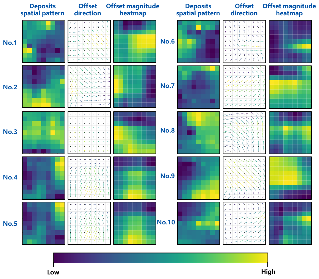
Figure 10 Comparison of offset direction and magnitude maps obtained by GK-CNN and GK-DCN with the geochemical patterns of ten mineral deposits clipped from PC2 score maps in this study. The yellow in the maps represent high concentration and high offset magnitude. The longer the arrow in the offset direction maps, the greater the offset.

CAM is a visualization technique used to reveal the image regions that DCN and CNN focus on when making decisions. It generates a heatmap by taking the feature maps of the last convolutional layer and performing a weighted summation. Bright areas indicate regions critical for predicting a specific class. The limitation of CAM is that it requires the network architecture to include a global average pooling layer. Grad-CAM is a generalization and enhancement of CAM. It overcomes the structural constraints of CAM by computing the gradients of the target class with respect to the feature maps of the last convolutional layer to obtain weights, generating a heatmap that localizes key regions of the image. This heatmap visually demonstrates which features the model focuses on to make predictions, thereby enhancing the model's interpretability. It allows us to intuitively understand the basis of the model's decisions and verify whether it focuses on reasonable features. Figure 10 displays the geochemical patterns corresponding to ten mineral deposits clipped from PC2 score maps, along with the Grad-CAM maps generated by the GK-CNN and GK-DCN models. As can be seen, GK-DCN, with their ability to adaptively adjust receptive fields, generate Grad-CAM maps that more accurately align with the spatial distribution patterns of actual geochemical spatial patterns. This indicates that the deformable network's ability to adjust the sampling locations of convolutional operations through offset modulation, which allows it to effectively capture complex and irregular geochemical patterns. Consequently, the deformable network demonstrates greater flexibility and accuracy in identifying geochemical spatial patterns. Their heatmaps clearly outline the spatially anisotropic distribution of geochemical fields, exhibiting higher spatial coupling with actual geochemical spatial patterns, and enhance the interpretability of model decisions (Fig. 11).

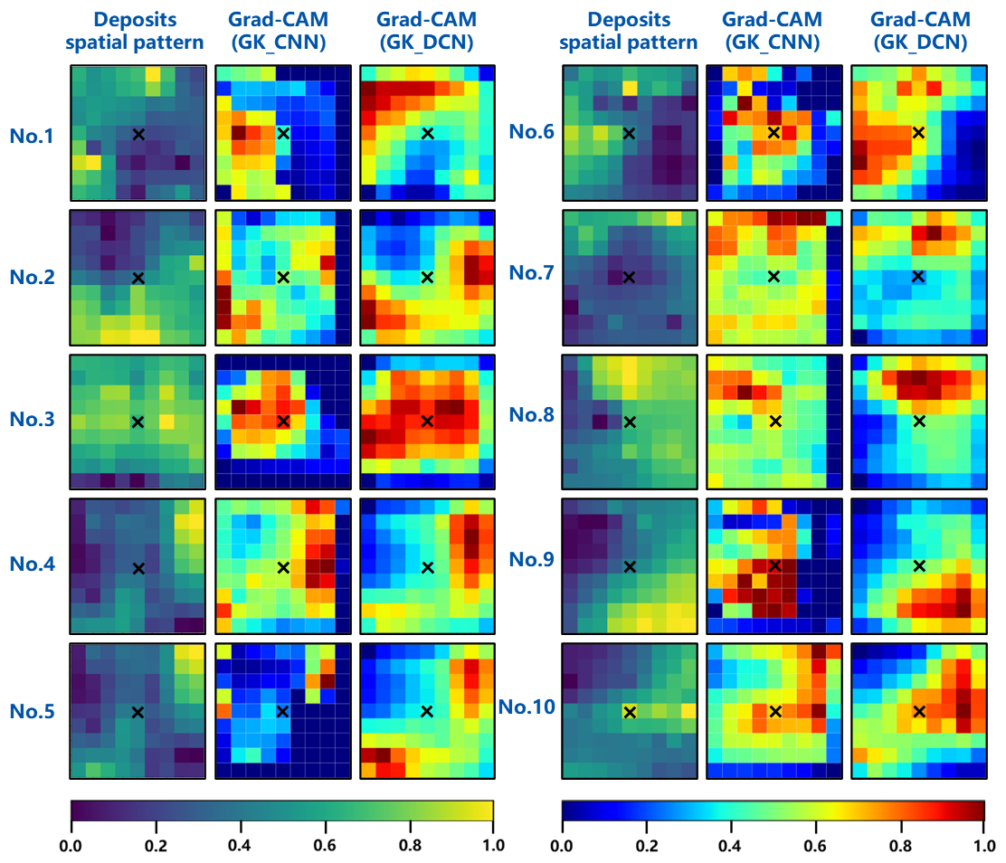
Figure 11 Comparison of Grad-CAM maps obtained by GK-CNN and GK-DCN with the geochemical patterns of ten mineral deposits clipped from PC2 score maps in this study. The yellow in the geochemical patterns of mineral deposits represent high concentration. The red highlighted regions in the Grad-CAM maps are the parts where models give more weight and contribute more the final classification. The black crosses represent the known deposits.

4.2 Comparative experiments

This section assesses the performance of our proposed model using seven metrics – Accuracy (ACC), Area Under the Curve (AUC), Kappa, Matthews Correlation Coefficient (MCC), Precision, Recall, and F₁, and compares it with models that are either non-geologically constrained or do not employ deformable convolution operation. The aim is to identify and interpret the performance differences (Chicco and Jurman, 2020; Powers, 2020). The metrics are defined as follows:

$$\begin{array}{}\text{(15)}& {\displaystyle }\mathrm{ACC}={\displaystyle \frac{\mathrm{TP}+\mathrm{TN}}{\mathrm{TP}+\mathrm{FP}+\mathrm{TN}+\mathrm{FN}}},\text{(16)}& {\displaystyle }\begin{array}{rl}& \mathrm{Kappa}={\displaystyle \frac{\mathrm{ACC}-P_e}{\mathrm{1}-P_e}};\\ & P_e={\displaystyle \frac{\frac{n}{\mathrm{2}}\left(\mathrm{TP}+\mathrm{FP}\right)+\frac{n}{\mathrm{2}}(\mathrm{FN}+\mathrm{FTN})}{n^{\mathrm{2}}}},\end{array}\text{(17)}& {\displaystyle }\begin{array}{rl}& \mathrm{MCC}=\\ & {\displaystyle \frac{\mathrm{TP}\times \mathrm{TN}-\mathrm{FP}\times \mathrm{FN}}{\sqrt{(\mathrm{TP}+\mathrm{FP})\times (\mathrm{TP}+\mathrm{FN})\times (\mathrm{TN}+\mathrm{FP})\times (\mathrm{TN}+\mathrm{FN})}}},\end{array}\text{(18)}& {\displaystyle }\mathrm{Precision}={\displaystyle \frac{\mathrm{TP}}{\mathrm{TP}+\mathrm{FP}}},\text{(19)}& {\displaystyle }\mathrm{Recall}={\displaystyle \frac{\mathrm{TP}}{\mathrm{TP}+\mathrm{FN}}},\text{(20)}& {\displaystyle }{F}_{\mathrm{1}}={\displaystyle \frac{\mathrm{2}\times \mathrm{TP}}{\mathrm{2}\times \mathrm{TP}+\mathrm{FP}+\mathrm{FN}}}.\end{array}$$

Here, true positive (TP), true negative (TN), false positive (FP), and false negative (FN) represent the agreement between the actual labels (true or false) and the classifier's predictions (positive or negative), with n denoting the total number of samples. The AUC corresponds to the area under the Receiver Operating Characteristic (ROC) curve, expressed as a proportion of the total area of the unit square. The ROC curve plots the true positive rate (TPR, or sensitivity) against the false positive rate (FPR, or 1 − specificity) (Fawcett, 2006).

Since the augmented training set (134 samples) is likely insufficient to support the generalization capability of the DCN and CNN with high-dimensional features (39 channels), and may increase the risk of overfitting. In order to verify whether these training data are sufficient to train the model without overfitting, we employed five-fold cross-validation (Kim et al., 2003; Lessmann et al., 2008). The dataset was randomly partitioned into five equally sized subsets. In each iteration, one subset served as the testing set, while the remaining four were used for training. This process was repeated five times so that every subset was used exactly once for testing. The final performance was evaluated by averaging the results from all five iterations. The results show that the predictive performance of the model on the testing set remains consistently high across all folds, with minimal fluctuations. This indicates that the model is well-trained without overfitting, demonstrating that the data are effective and sufficient for model training (Fig. 12).

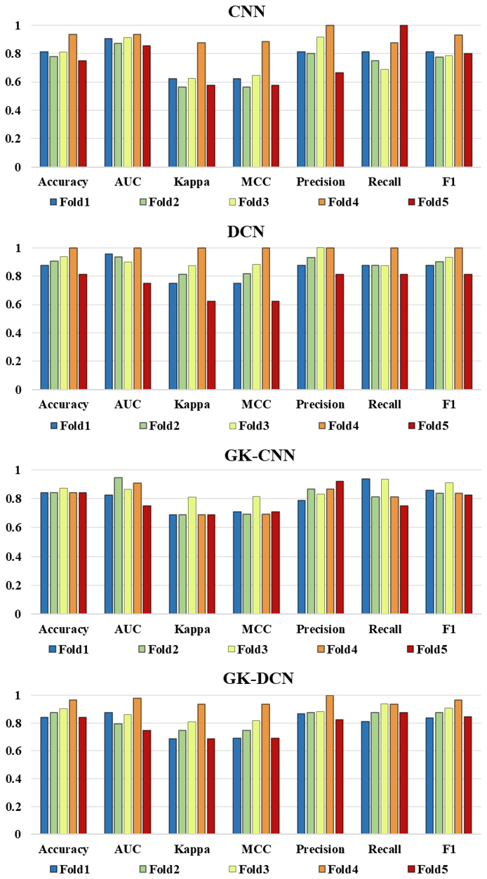
Figure 12 Results of five-fold cross-validation for models CNN, DCN, GK-CNN, and GK-DCN across different performance metrics.

Figure 13 is a comparative performance analysis of CNN and DCN in geochemical anomaly recognition tasks based on seven performance metrics. The radar chart comparison clearly shows that the DCN outperforms the standard CNN in the vast majority of performance metrics, demonstrating superior overall performance. In terms of recognition accuracy and reliability, DCN exhibits significant advantages. Its higher accuracy indicates a stronger overall prediction correctness and greater certainty in positive class predictions. In terms of model discriminative ability and error control, DCN also leads. Its larger AUC indicates a stronger ability to distinguish between positive and negative samples. Additionally, DCN's lower false positive rate (FPR) means fewer false alarms where normal samples are misclassified as anomalies, which is crucial in practical applications emphasizing safety and efficiency. In summary, due to its deformable convolutional structure, DCN can adaptively adjust the receptive field and more accurately capture the irregular and complex spatial features of anomalies. This enables a comprehensive outperformance over traditional CNN across most of metrics, particularly in reducing missed detections (high recall) and lowering false alarms (low FPR). This demonstrates DCN's stronger applicability and robustness for complex anomaly recognition tasks (Fig. 13).

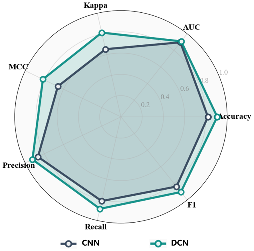
Figure 13 Evaluation of model performance between CNN and DCN in Accuracy, Precision, Recall, F₁-score, AUC, Kappa, and MCC.

The model must prioritize not only accuracy but also geological consistency. The radar plot compares its geologically constrained counterpart (GK-CNN and GK-DCN) (Fig. 14). While both models demonstrate excellent predictive capabilities, GK-CNN and GK-DCN, which incorporates geological knowledge directly within the model architecture, outperformed the unconstrained CNN and DCN. This is evident in key metrics, where the knowledge-enhanced model achieved higher performance while successfully integrating geological constraints. The experimental results demonstrate that incorporating geological knowledge as a physics-based regularization term within the loss function significantly boosts pattern recognition performance and model interpretability. This geologically constrained model effectively identifies potential mineral deposits by guiding training optimization to recognize anomalies associated with ore-controlling faults, enhancing learning and generalization capabilities.

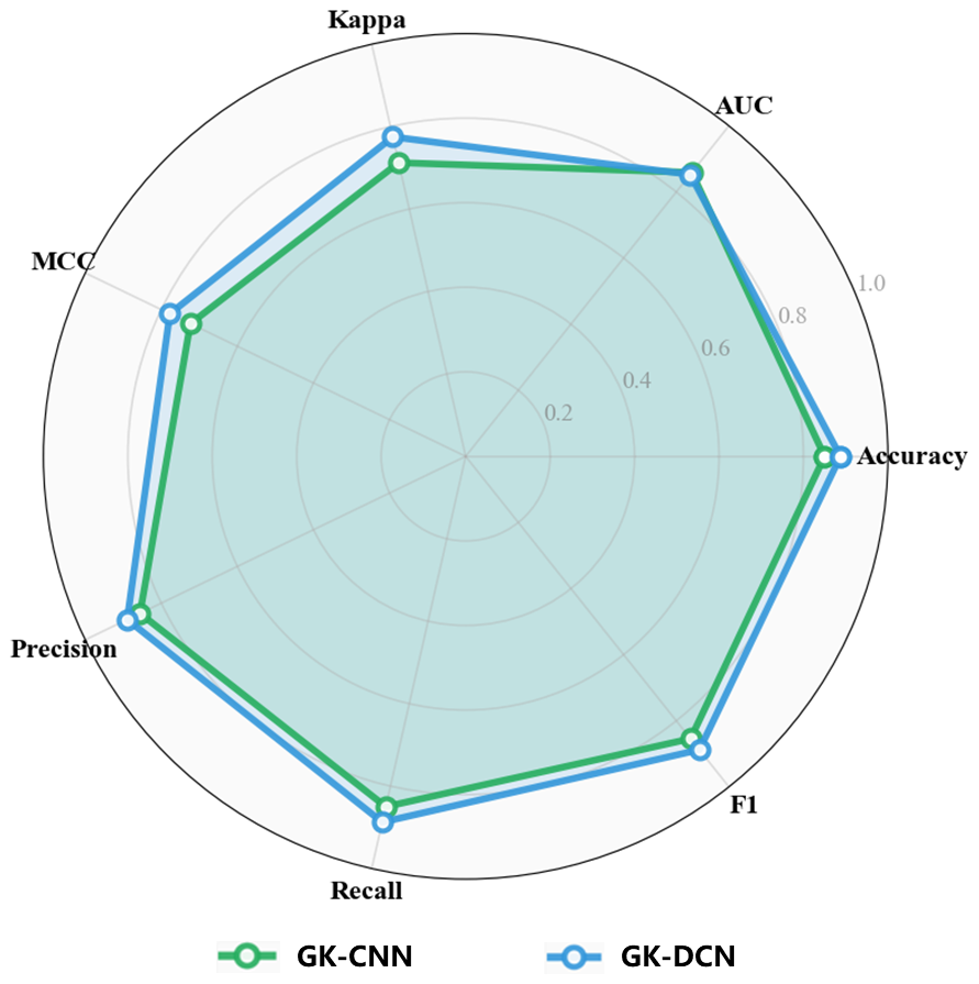
Figure 14 Evaluation of model performance between GK-CNN and GK-DCN in Accuracy, Precision, Recall, F₁-score, AUC, Kappa, and MCC.

A primary limitation of this work lies in the interpretability and completeness of the incorporated geological knowledge. The current model leverages observed ore-controlling faults as a geological constraint within the loss function. This approach, while enhancing the model's focus on anomalies related to observable structures, inherently introduces a significant bias. It assumes the spatial patterns of geochemical anomalies are predominantly controlled by these mapped faults. Consequently, in exploration scenarios for covered areas or deep-seated mineral deposits, such as in southern Tianshan Au-Cu polymetallic ore district, the model's performance is constrained. It may suppress or fail to recognize valid geochemical anomalies that are spatially associated with blind or concealed faults, which are not observable at the surface but are equally crucial ore-controlling factors. This limits the model's generalizability and predictive power in covered regions where observed structures are not fully indicative of subsurface controls.

5 Conclusions

This study introduces deformable convolutional neural networks into the field of geochemical anomaly identification to address the issues in capturing irregularly shaped anomalies within complex geological backgrounds. The adaptive receptive field adjustment capability of deformable convolution units enables more precise capture of the spatial distribution characteristics of geochemical anomalies in complex geological settings. This enhances the model's ability to learn and represent geochemical spatial distribution features, thereby achieves superior anomaly identification results. Experimental results demonstrate that, compared to conventional convolutional neural networks, this method significantly improves accuracy and spatial continuity in anomaly identification, allowing more effective separation of mineralization-related anomalous information from high-dimensional, nonlinear geochemical data.

Prior knowledge of ore-controlling faults is incorporated into the model's loss function as a constraint. The fault-constrained loss function effectively guides the network's learning process, resulting in the identified geochemical anomalies exhibiting higher spatial alignment with known ore-controlling faults. This enhances the geological significance of the anomalies, reduces interference from the geochemical background field, and improves the accuracy of anomaly identification.

The interpretability of the model is further examined through visualizations of the learned offsets and Gradient-weighted Class Activation Mapping. First, the visualization of the offset fields learned by the deformable convolution kernels clearly reveals the network's adaptive receptive field adjustment behavior. The learned offset vectors effectively point to key anomalous spatial structures and irregular trends in the geological mineralization process, serving as important quantitative indicators of anomaly irregularity. Second, Gradient-weighted Class Activation Mapping intuitively demonstrates the key regions, where the model focused during decision-making. The highlighted areas in the heatmap show strong overlap with known mineral deposits and high anomaly zones, providing compelling evidence for the “black-box” decision-making process and demonstrating the model's focus on geochemical features related to mineralization. In summary, this study not only validates the effectiveness of combining deformable convolution with geological prior knowledge in geochemical anomaly identification but also provides a window into understanding the model's decision-making process through offset and Grad-CAM visualizations, significantly enhancing the accuracy and interpretability of AI models in geochemical data processing. This method offers a new tool for deep learning-driven geochemical data analysis and holds practical value for future geochemical exploration.