Accumulation-based Runoff and Pluvial Flood Estimation Tool (AccRo v.1.0)

Knowledge about spatially distributed inundation depth and overland flow quantities, as well as related flow velocities, is critical information for establishing a pluvial flood forecasting system and the related disaster management. This kind of information is often derived from computationally demanding simulations with 2-dimensional hydrodynamic models, limiting the number of scenarios for which information can be provided and challenging real-time forecasting. To address this gap, we developed the model AccRo (Accumulation-based Runoff and Flooding), which is a computationally efficient method to derive maximum inundation depth, maximum flow velocity and maximum specific discharge of a flood event at larger spatial scales, based on an improved flow accumulation method to better represent the spatial extent of inundated areas. To assess the quality of AccRo, we compare the results from the AccRo model with the results of two different state-of-the-art 2-dimensional hydrodynamic models for design cases as well as real-world pluvial flood examples. We find that AccRo is able to represent both, the analytical solution for the design cases and the simulations of the hydrodynamic models in the real-world example in high quality, well within the range of the two hydrodynamic models. In combination with the low computational requirements, we conclude that AccRo is a valuable tool for assessing pluvial flood hazards, typically based on peak conditions of water depths, discharges and flow velocities as well as the maximum spatial extend of flooded area.

1 Introduction

Pluvial floods have large damage potential as is demonstrated by recent catastrophic events like the pluvial flooding in Texas in July 2025 or the floods in Spain from October 2024. They are expected to become more frequent and more intense in the light of global change (e.g. Skougaard Kaspersen et al., 2017). So far, however, warning mechanisms for pluvial floods are rather limited. This is on one hand due to the random nature and fast build-up phase of extreme convective precipitation events (e.g. Li et al., 2021), although probabilistic ensemble forecasts might improve the forecast quality (e.g. Bouttier and Marchal, 2024). On the other hand, there is also the issue of computational resources and adequate lead times connected with the identification of inundation areas. This is especially important for the real-time warning of pluvial floods in suburban and urban regions, often characterised by a relatively strong role of hydrological processes and relatively large accumulation areas, requiring a more holistic approach to include the impact of runoff generation and hydraulic effects into a warning.

Because this is not yet available, a widely used concept to support pluvial flood risk assessment as well as a baseline for planning emergency management options are so-called pluvial flood maps (e.g. Wimmer and Hovenbitzer, 2025). These maps depict potential inundation areas for certain design rainfall events based on the output of hydrological and/or hydrodynamic models (Bulti and Abebe, 2020). A step towards issuing a real-time warning of pluvial floods was recently made with the concept for a mesoscale pluvial flood index (PFI) to depict the current hazard of a region being flooded (Weiler et al., 2025). The PFI builds on the spatial extent of flood hazard areas in a certain region. These are defined as areas where the flood poses a danger for people's life. Key variables for most pluvial flood maps as well as the PFI are the maximum inundation depth and maximum surface flow velocity. The PFI also takes into account the maximum specific discharge. To accurately represent hazard areas, the spatial resolution of the data must be fine enough to represent important flow structures in urban areas (e.g., buildings, streets, underpasses, etc.) as well as in the surrounding areas (farm and forest roads, small creeks, etc.), which frequently deliver water into settlements.

The above-mentioned variables are also a standard output of 2-dimensional (2d) hydrodynamic models. However, especially when targeting a larger regional scale (e.g. when focusing on sub-urban cases with large accumulation areas of 10–100 km² or in the case of deriving the PFI) the high computation costs and integration times of 2d hydrodynamic models might become a bottle neck for real-time forecast. Although there are recent developments like GPU based 2d-hydrodynamic models (e.g. RIM2D, Apel et al., 2024, or IBER-Plus, Moraru et al., 2023 or SCENARIFY, Buttinger-Kreuzhuber et al., 2022) or the use of ANN for instant forecasting (e.g. Berkhahn et al., 2019), both approaches are bound to huge computation efforts either for the real time simulation in the case of the GPU models or in the preparation of extensive training data for the ANN models. Especially for mixed regions with larger influence of non-urban areas and diverse hydrological responses, the training of ANN requires a very large dataset (e.g. Reinecke et al., 2024). In the case of hydrodynamic models, one has to be aware of the fact that the computational performance strongly depends on the individual characteristics of the simulated case. The main limitation arises when large domains include localized features (e.g. gullies, small rills) that require fine spatial resolution, leading to small model time steps and many operations in order to keep the models numerically stable.

On the other hand, there are computationally efficient GIS-based methods available to simulate the flow accumulation in a very reasonable time also for larger areas (Avila-Aceves et al., 2023). However, there are some shortfalls, which are mainly that the outputs of these methods do not fulfil the data requirements for estimating the pluvial flood maps, since they only provide accumulated flow amounts but no explicit measure for inundation depths or flow velocities. Furthermore, spatial structures of inundated areas extracted from flow accumulation methods are often much more spatially confined than the ones from 2d-hydraulic models. Although accumulation-based methods exist that try to mimic the spatial extent of inundated areas depicted in hydraulic models (e.g. FastFlood, van den Bout et al., 2023) they do not yet provide the spatial details needed to define local flood hazard areas. Furthermore, approaches like FastFlood gain their computational efficiency partly due to simplifications like the assumption of constant rain rates, hence requiring subsequent empirical corrections based on event and catchment characteristics (e.g. an empirical catchment shape factor) to somehow mimic real cases. Since AccRo directly incorporates the temporal and spatial event dynamics into the simulations, there is no need for any empirical correction mechanisms in our model.

In order to obtain a fast estimate of the spatial pattern of maximum water depth, maximum flow velocity and maximum specific discharge at a reasonable spatial resolution allowing us to represent important obstacles as buildings and preferential flow paths (e.g., roads and ditches), we developed the raster-based model AccRo (Accumulation-based Runoff and Flooding). This novel approach combines the benefits of the computationally fast flow accumulation approaches with the representation of event and site characteristics to yield local flood hazard areas comparable to 2d hydrodynamic model results. Key elements of AccRo are the iterative flow accumulation making AccRo calculation times independent of spatial resolution and connected model internal time steps as well as the development of robust functions to link accumulated flows to key information required in flood hazard assessments. In our study, we first describe the methodological details of the AccRo and the validation framework we used to compare the AccRo output with 2d hydrodynamic models, followed by the validation of the results.

The paper is structured as follows. In Sect. 2 we describe the methodological details of AccRo as well as the validation framework used to verify AccRo output in comparison to 2d hydrodynamic models. In Sect. 3 the results of the validation are presented. Section 4 provides a discussion of the findings and suggestions for possible further improvements. The paper ends with a conclusion section.

2 Method

2.1 Relating accumulated runoff (A_s) to q, w and v

Central element of AccRo is the flow accumulation function (FAF) of the Python module richDEM (Barnes, 2016). FAF is a very fast method yielding reliable results, for quantifying flow accumulation with a choice of several flow direction approaches like convergent methods, such as D8 (O'Callaghan and Mark, 1984) or divergent methods, like Quinn method (Quinn et al., 1991). One major advantage in using FAF is that it allows the use of accumulated weights based, e.g., on area or in our case on surface runoff intensities (s). Applying FAF with s as a weighting factor yields to spatially distributed estimates of total surface runoff flowing through a raster cell depending on the input s and the flow paths, according to the digital elevation model (DEM). To use FAF to estimate maximum inundation or water depth (w), maximum flow velocity (v) and maximum specific discharge (q), cumulative surface runoff (A_s) must be translated into the appropriate target variables. Furthermore, the accumulation of s in FAF is only controlled by the DEM, ignoring the need to account for changing hydraulic conditions caused by varying water depths. As a result, the second critical element in AccRo is the decoupling of the accumulation from the DEM surface when hydraulic conditions and flow direction change due to varying water depth.

As previously stated, using FAF with s as the weighting factor returns A_s. The temporal development of A_s in a specific cell, however, is not incorporated by FAF. Knowing the travel times is key to estimating q, w and v, thus we have to include the temporal perspective into AccRo. For a given raster cell, we can distinguish between the time a water parcel needs to flow though the cell (t_c) with cell length l, the forward time i.e. the time the water parcel needs to reach another cell (typically the outlet), and the backward flow time (t_b), which is the duration of flow in a single cell caused by delayed inflow from cells further uphill (see Fig. 1). In general, t_b will be shorter on top of hills or convex structures (less cells accumulated) and larger in valleys and reaches the maximum value at the catchment outlet. The concepts for t_b and t_f are widely used in hydrology, e.g. t_b for water age calculations (Benettin et al., 2015) and pollutant transport (Zhang et al., 2024) and t_f for isochrones and hydrographs estimations (Olivera and Maidment, 1999; Saghafian et al., 2002).

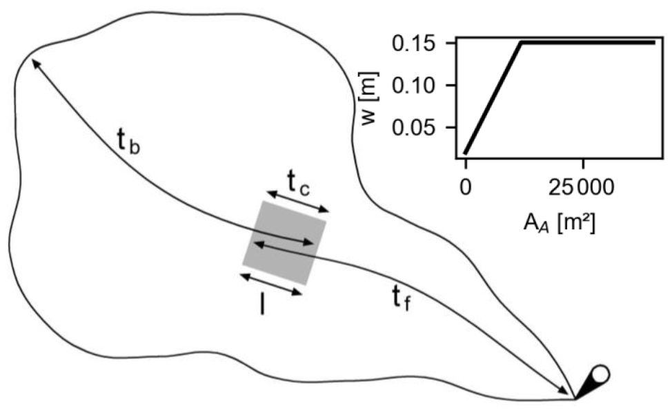
Figure 1 Scheme of the definitions of relevant times a water parcel travels in a catchment and the assumed initial relationship between water depth and area weighted flow accumulation.

2.1.1 Spatially distributed estimation of backward flow time (t_b)

For a given water depth, the flow velocity (v_c) and hence the flow time (t_c) through a raster cell can be derived from the slope and hydraulic radius based on the Gauckler-Manning-Strickler (GMS) equation:

$$\begin{array}{}\text{(1)}& {\displaystyle }{v}_{\mathrm{c}}=k\times R^{\frac{\mathrm{2}}{\mathrm{3}}}\times i^{\mathrm{0.5}}\text{(2)}& {\displaystyle }{t}_{\mathrm{c}}={\displaystyle \frac{l}{v_{\mathrm{c}}}}\end{array}$$

with k – Strickler surface roughness [L${}^{\mathrm{1}/\mathrm{3}}$ T⁻¹], R – hydraulic radius [L] – in our case water depth in a cell, i – slope [L L⁻¹], and l – cell length [L].

The slope is derived from the DEM and the roughness values can be estimated from spatially explicit land-use or surface cover information (e.g. LUBW, 2016). Adding up t_c along a flow path from the top to the bottom (top-down approach) yields the backward flow time (t_b) for each cell along this flow path, which represents the duration of flow in a cell caused by flow times from upslope cells finally draining through the given cell (see Fig. 1 for schematic). Since our method is designed for events with rather high s values (pluvial flood events), we initially estimate t_c (and hence also t_b) only for water depths between 2 and 15 cm. To assign an initial water depth (w_c) for the calculation of t_c, we develop a simple linear relationship (see Eq. 3) between the w_c and area weighted flow accumulation (A_A) derived from FAF using the Quinn Method, with an intercept equal to 2 cm (w_sf) and a slope of 1 × 10⁻⁵ m⁻¹ (see inlet in Fig. 1). The reason for using the Quinn Method for area and runoff weighted accumulation is that it is a divergent method representing flow processes, which is more realistic than convergent methods on hillslopes and in valleys. Flow occurs to all downslope neighbours proportional to i and to the tangent of the angles. w_sf is the water depth under which we assume sheet flow (HLNUG, 2020). The slope represents the quotient of a water depth (w_r) above which we assume that roughness is independent of changes in water depth (i.e. larger than 10 cm) and a critical accumulation area of 10 000 m² ($A_{{\mathrm{A}}_{\mathrm{crit}}}$). For $A_{{\mathrm{A}}_{\mathrm{crit}}}$ we consider that the entire area would generate runoff, the resulting water depth reaches values of 10 cm (w_r) or more due to the accumulation. As previously stated, the maximum is set to 15 cm. The use of this linear equation yields only catchment or area-specific results that are unaffected by a specific runoff event.

$$\begin{array}{}\text{(3)}& w_{\mathrm{c}}=\left\{\begin{array}{cc}\mathrm{0.02}\mathrm{m}& w_{\mathrm{c}}<\mathrm{0.02}\mathrm{m}\\ \frac{w_{\mathrm{r}}}{A_{\mathrm{crit}}}\times A_{\mathrm{A}}+w_{\mathrm{sf}}& \mathrm{0.0}\mathrm{2}\mathrm{m}\le w_{\mathrm{c}}\le \mathrm{0.15}\mathrm{m}\\ \mathrm{0.15}\mathrm{m}& \mathrm{0.15}\mathrm{m}<w_{\mathrm{c}}\end{array}\right.\end{array}$$

Having defined the cell-specific t_c we now have to identify for each cell all upslope cells eventually draining into the cell of interest to calculate the backward flow time t_b. For the top-down approach (starting with the highest DEM value), we use a sink-filled DEM (modified with the richDEM epsilon filling module, Barnes et al., 2014) as a baseline for an area-weighted D8 accumulation. We use the convergent D8 method of FAF here, since we just want to select the upslope cell with the largest inflow and thus the most relevant t_b value. t_b in a cell is then the sum of t_c in this cell and the relevant t_b value upslope. To find the most relevant upward t_b value of the neighbouring eight cells, we queried four criteria to select the relevant t_b of the eight neighbouring cells:

1. DEM value is higher,

2. D8 accumulation is lower,

3. of all neighbours that fulfil criteria (1) and (2) D8 accumulation is maximal,

4. of all neighbours that fulfil criteria (1) and (2) t_b is maximal.

Since not all 4 criteria are always fulfilled, the importance decreases from (1) to (4). If criterion (2) is not fulfilled, a D8 accumulation weighted t_b of all neighbours fulfilling (1) is used as a replacement. If even criterion (1) is not fulfilled, criteria (2) and (3) are applied to neighbours with equal DEM values. Figure 2 exemplarily shows for a small catchment (ca. 3 km²; see Sect. 2.4 and Fig. 6 for more details) the spatial distribution of the variables used to calculate t_b (panels a to c) as well as the resulting t_b (Fig. 2d).

Figure 2 Example of spatially distributed variables to calculate backward flow time in a small catchment (see Sect. 2.4). (a) Area flow accumulation (m²); (b) Area specific water depth (m); (c) cell flow time (s); (d) backward flow time (s).

2.1.2 From surface runoff accumulation to cell-specific maximum discharge using backward flow time

In the previous section, we showed how to calculate for each raster cell an event-independent backward flow time t_b. However, in order to determine the maximum specific discharge q_max at a particular cell, we must connect this data to the event-specific s response and the accumulated surface runoff A_s. In essence, the following principle guides the estimation of q_max:

$$\begin{array}{}\text{(4)}& q_{\max }=A_{\mathrm{s}}\times l\times F\left[{\mathrm{L}}^{\mathrm{3}}\right(\mathrm{T}\cdot \mathrm{L}{)}^{-\mathrm{1}}]\end{array}$$

respectively surface discharge per cell

$$\begin{array}{}\text{(5)}& Q_{\max }=A_{\mathrm{s}}\times l^{\mathrm{2}}\times F\left[{\mathrm{L}}^{\mathrm{3}}{\mathrm{T}}^{-\mathrm{1}}\right]\end{array}$$

where F [1 T⁻¹] represents the factor to transfer A_s [L] to q_max [L³ T⁻¹] and l [L] the cell size.

The next section provides additional details concerning the estimation of F (see Fig. 3 for an example). We start with the most basic scenario: a raster cell with no inflows from neighbouring cells, such as the top of the hill at the watershed boundary. In this case, the temporal response of generated runoff s of the specified cell (see Fig. 3a) is equal to the response of surface runoff. The maximum s is equivalent to the maximum surface discharge. In this case, t_b equals t_c, with t_c getting closer to zero as the cell size decreases (i.e., it is 0 for a point). In this scenario, F is the quotient of the cell-maximum value of s (s_max) and the product of its discrete time unit (Δt) and its sum (∑s) (see Eq. 6).

$$\begin{array}{}\text{(6)}& F={\displaystyle \frac{s_{\max }}{\sum s\times \mathrm{\Delta }t}}\end{array}$$

Figure 3 Example of how F is developing in dependence of s and t_b.

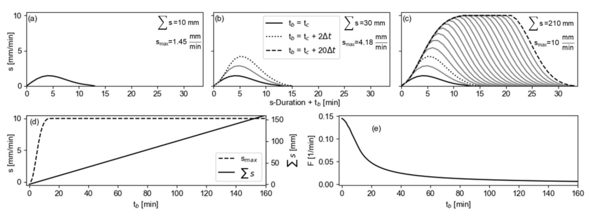
However, the situation is different for cells that receive inflow from neighbouring cells. In this case, t_b is greater than t_c, and we obtain distinct overlapping s responses. The degree of overlap depends on the chosen time step of s (since s is an intensity). As a result, s_max and ∑s change for cells with t_b>t_c (Fig. 3b). A particular cell's ∑s (and A_s) will increase with its t_b, which essentially indicates that more cells will eventually inflow into the cell. For cells with larger t_b, F gradually decreases because s_max reaches a maximum at a specific t_b and will not increase further due to the delayed runoff from the inflow cells. (Fig. 3c)

To visualise the evolution of s_max, ∑s and F with increasing t_b in Fig. 3, we defined an exemplary flow path. In Fig. 3a, t_b equals t_c, s_max= 1.45 mm min⁻¹ and $\sum s=$ 10 mm and so F= 0.145 min⁻¹. In Fig. 3b–c we increase t_b (2 and 20 min) and the corresponding s response. The shift of overlap is defined by the underlying time step of the intensity. So in Fig. 3b, t_b equals t_c+ 2 min, s_max= 4.18 mm min⁻¹ and $\sum s=\mathrm{30}$ mm and so F= 0.14 min⁻¹ and in Fig. 3c, t_b equals t_c+ 20 min, s_max= 10 mm min⁻¹ and $\sum s=\mathrm{210}$ mm and so F= 0.048 min⁻¹. Calculating this for all possible t_b in a catchment, we receive a continuous curve for s_max, ∑s (Fig. 3d) and F (Fig. 3e) in dependence of t_b. Based on this explanation, it is evident that F does not depend on the time unit of s. However, the F factor changes if the quantity and/or duration of the response varies.

As the spatial and temporal variability of s is relevant for deriving the F curve, the response of s should represent an average response over a specific area. This is usually not fulfilled anymore if the area is becoming too large since the variability in individual s responses will significantly vary due to different spatial factors influencing the runoff generation, such as vegetation, soil type, moisture, and precipitation. Hence, we target for a size of around 2 × 2 km² for which a specific response of F is valid. This area can be e.g. a small catchment, some part of a catchment or the area covered by a grid cell from radar-based precipitation input.

2.1.3 From maximum specific discharge to maximum water inundation to maximum flow velocity

With the assumption that q, w and v are related to each other, it's now possible to calculate w and v based on q using Gauckler-Manning-Strickler equation for each cell (see Eq. 1). Since the hydraulic radius (R) is not known, we assume that the cross-sectional width is large compared to water depth, and so we set R equal to w. On hillslopes this assumption is mostly given, but in channels this assumption might lead to higher velocities.

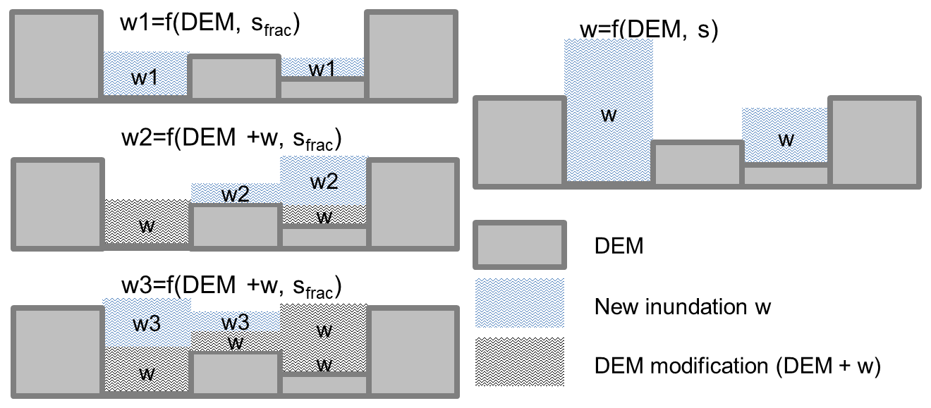
Figure 4 Schematic illustration of the iterative process. Left: s_frac is accumulated in three iterations, altering the DEM with the resulting inundation and therefore changing the accumulation location of each iteration. Right: s is accumulated once without altering the DEM.

By rearranging Eq. (1) we get

$$\begin{array}{}\text{(7)}& Q=v\times C=k\times R^{\frac{\mathrm{2}}{\mathrm{3}}}\times i^{\mathrm{0.5}}\times C\end{array}$$

and with R=w and

$$\begin{array}{}\text{(8)}& C=w\times l\end{array}$$

we get

$$\begin{array}{}\text{(9)}& w={\left({\displaystyle \frac{\frac{Q}{\mathrm{1000}}}{i^{\mathrm{0.5}}\times k\times l}}\right)}^{\mathrm{3}/\mathrm{5}}\end{array}$$

with C – cross-sectional area of flow [L²] and l – cell size [L].

2.2 Representation of changing hydraulic conditions due to inundation

As already introduced before, the use of FAF typically results in water accumulation, either adhering to the steepest descent in the D8 approach or encompassing all downward gradients for diverging methods, resulting in relatively small inundated areas. Hydraulic models, on the other hand, attempt to simulate reality by allowing flowing water to initially fill structures such as channels, hollows and sinks before eventually overflowing banks or other structures, resulting in different flow pathways due to the adapting water depths as compared to the initial DEM structures. As a result, the flow accumulation analysis should take into account shifting hydraulic conditions in order to mimic more natural inundation processes.

We use spatially distributed surface runoff (s) generated from a hydrological model as a weighting factor in the FAF. The quantity and location of computed accumulated runoff (A_s) are determined by the flow direction defined by the DEM and the spatial pattern of s. To allow for the expansion of flow pathways in AccRo to mimic the inundation processes, the accumulation is done iteratively by partitioning the total amount of s into n equal fractions (s_frac). Utilising the previously established methodology for calculating q (Eq. 4) from the generated A_s, we can calculate w for each cell based on q after each iteration. Adding w after each iteration to the elevation before the iteration, we can produce a modified DEM surface, with certain regions already inundated. This adjusted DEM is then the new reference for the FAF in the next iteration step. By repeating this procedure for multiple iteration steps, the accumulated surface runoff generates larger inundated areas and levels out the cross sections (see schematic example in Fig. 4), in contrast to calculating A_s only once without modifying the DEM (Fig. 4 right column).

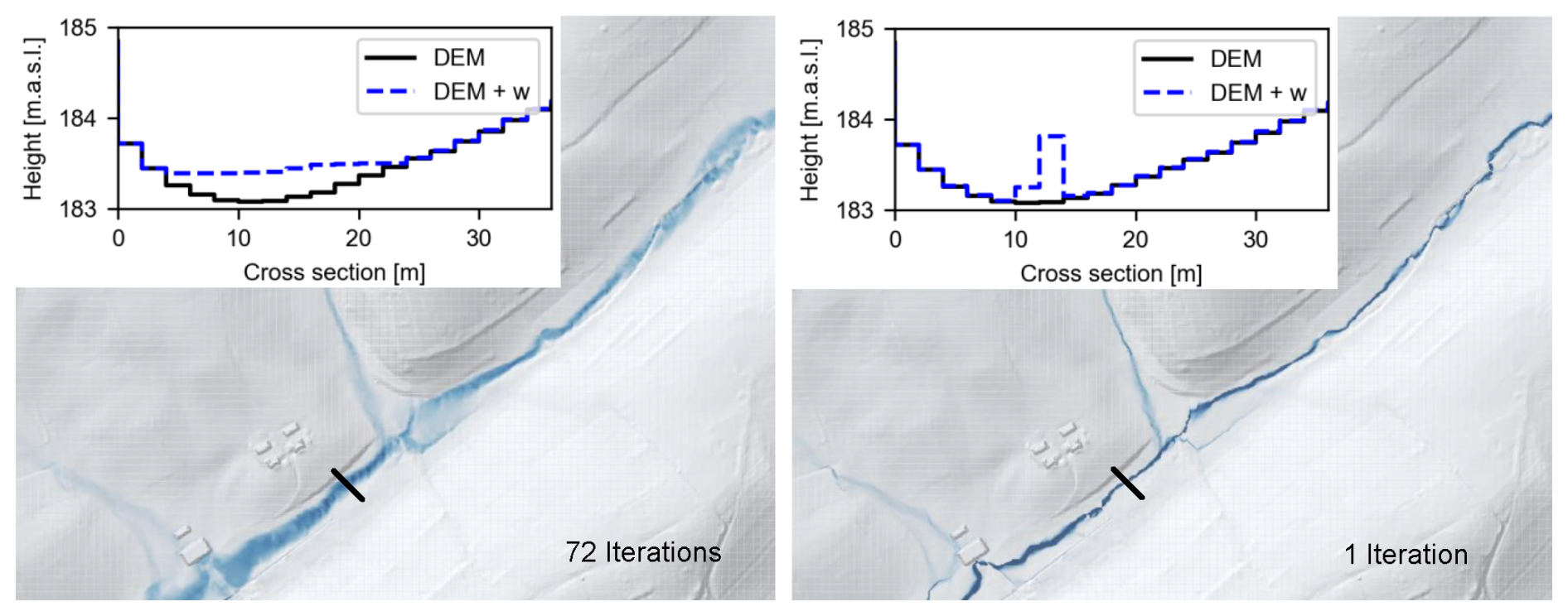
Figure 5 Results of the iterative approach. Left: inundation in meter when 72 iterations are applied, right inundation when one iteration is applied. The sum of s is the same for both simulations. The black line in the centre represents the location of the cross section.

Figure 5 depicts the spatial effect of the iterative flow accumulation procedure for the example of a small test catchment (see Fig. 6 for details). The maps show the maximum inundation after 72 iterations (left) and the setup where s is accumulated only once (right). Note that the sum of s is the same for both examples. Narrow structures become more extended structures and additional regions become flooded with more iterations. We additionally included the water depth at a specific cross section (small inlet figures) to highlight the iteration setup and the resulting inundation, whereas in the case without iteration an unrealistic water hill builds up.

Figure 6 Overview of the setups used in the validation framework. The panels (a) and (b) depict the upper parts of the design setup with a hillslope (a) and channel (b) case. The blue lines on the top represent the location of constant s input, the arrows indicate predominant flow directions. The small inlet figures on the upper right (hillslope) and lower left (channel) provide an overview on the dimensions of the two case studies. The real-world catchment Riedgraben is depicted on the right-hand side (c). Here the shadings indicate the Strickler roughness values.

While q and w are calculated for each iteration step and then added up to determine the respective maximum values, v is not calculated throughout the iteration process. As a result, only one computation of v is performed after the iteration process using Eq. (1). To account for changes in slopes caused by inundated areas, we recalculate i by incorporating w, which means that the slope is now determined by the gradient of the water surface (DEM plus inundation depth).

2.2.1 Sinks

For handling sinks, we generally have two approaches available. Sinks may be excluded by pre-filling them prior to the iteration, or they may be included and subsequently filled during the iterative process. For the latter, the locations and volumes of sinks are calculated by subtracting the non-filled from the filled DEM. To avoid redistributing of a too large amount of s inside a sink, only A_s of cells representing the local DEM minima in sinks for the relevant iteration step are considered. Redistribution of water within sinks is done by an internal sink iteration routine. This routine redistributes the water within the sinks to level out DEM plus water depth, ensuring that no cells outside of the sink are affected. Surplus water, or inundation that exceeds the sink depth, is added to s_frac in the subsequent iteration step.

2.2.2 Defining the number of iterations

As shown in Figs. 4 and 5, the spatial expansion of the inundation area potentially increases with the number of iterations.

The optimal number of iterations, however, is not a fixed value but depends on catchment and event characteristics. In order to produce realistic results in rather flat regions, more iteration steps are needed than in regions with greater topographical variation. Furthermore, higher runoff intensities require more iteration steps than lower intensities. To consider these aspects, AccRo initially estimates the portion of total runoff that would generate a maximum inundation of 10 cm in an accumulation area of 10 km² at one iteration. For this purpose, a single initial run with only one iteration of normalised total runoff s × max(s)⁻¹ is computed. To calculate the number of iterations n, the resulting (spatial) maximum inundation depth is divided by 0.1 m and multiplied by the maximum total runoff as shown in Eq. 9.

$$\begin{array}{}\text{(10)}& n={\displaystyle \frac{\max \left(w\right)}{\mathrm{0.1}}}\times \max \left(s\right)\end{array}$$

We evaluated this approach for different regions and various cases with different runoff intensities. We discovered that when n exceeds 100, the findings become quite identical. As a result, we set n_max to 120 and n_min to 12, allowing for some spatial expansion under low runoff amounts.

Table 1 Summary of selected rainfall and runoff event characteristics.

Table 2 Model results of the hillslope scenario; specific discharge at steady state is 40 liter (m s)⁻¹. w and v are calculated with Gauckler–Manning–Strickler with i= 0.03, k= 50, 26.5, 10 m${}^{\mathrm{1}/\mathrm{3}}$ s⁻¹ and q= 40 liter (s)⁻¹ (cross-sectional flow width ≫ water depth).

^* Simulation did not stabilize.

2.3 Estimation of flood hydrographs

As a by-product of our approach in AccRo, we can also derive the flood hydrograph at defined locations. We use the idea of the geomorphological instantaneous unit hydrograph (GIUH) (e.g., Rigon et al., 2016) and the estimated maximum flow velocity as well as the water volume stored in sinks to calculate the flood hydrograph. For this, we use v to calculate the forward flow time (t_f) to a given location in the catchment (in general the outlet, but can be any) with the SAGA module “ta_hydrology” (Maximum Flow Path Length) (Conrad et al., 2015). The amount of water retained in sinks is used to reduce the response of s i.e. input into GIUH. As v is the maximum velocity of the underlying event, one can expect that the derived flood hydrograph is faster compared to a hydrograph of a 2d hydrodynamic model.

2.4 Validation framework

Since pluvial floods usually inundate areas outside streams and channels, measured data of flooding extent or inundation depths as well as flood hydrographs for different rainfall runoff events are rare. Hence, instead of using real observations, we evaluate AccRo with model simulations of two hydrodynamic models: HydroAs version 6.2.2 (Hydrotec, 2025) and RIM2D (Apel et al., 2024, Version Jan 2025). Although we are aware of the fact that this does not necessarily represent the ground truth, currently it seems the best approach to get an estimate of the quality of the AccRo simulations.

To evaluate the quality of AccRo results, we defined different scenarios, for which we conducted simulations with the three different models. First, we simulated artificially created hillslopes under steady-state situations (Fig. 6a, b), where analytical solutions can be derived. Second, we simulated pluvial flooding in a real-world catchment (Fig. 6c).

For the artificial situations, we simulated overland flow on a planar hillside (1000 by 2000 m) with a constant slope of 0.03 m m⁻¹ (see Fig. 6a). For the second situation a channel of 2 m width is located between two declining surfaces (with a constant slope of 0.03 m m⁻¹) with an overall slope along the channel axis of 0.03 m m⁻¹. In both cases the cell size is 1 × 1 m², and a constant input of s was only applied along the uppermost rows (see blue lines in Fig. 6a and b). For the channel experiment, the total input was set to 1 m³ s⁻¹ but distributed equally along the upper row. When steady state is reached, this value should be found in the channel. For the hillslope experiment, s was set to a constant value of 40 liter s⁻¹ per cell for a width of 500 m on the top of the hillslope. The simulation time was long enough so that steady-state conditions could be reached. In both cases, a constant roughness over the entire domain was assumed; however, we repeated the simulation using different roughness estimates.

Table 3 Model results of the designed channel situation; specific discharge at steady state is 1 m³ (s ⋅ m)⁻¹. w and v are calculated with GMS equation with i= 0.03, k= 50, 26.5, 10 m${}^{\mathrm{1}/\mathrm{3}}$ s⁻¹ and q = 1 m³ s⁻¹ (cross-sectional flow width = channel width = 2 m). Cell size is 1 × 1 m² .

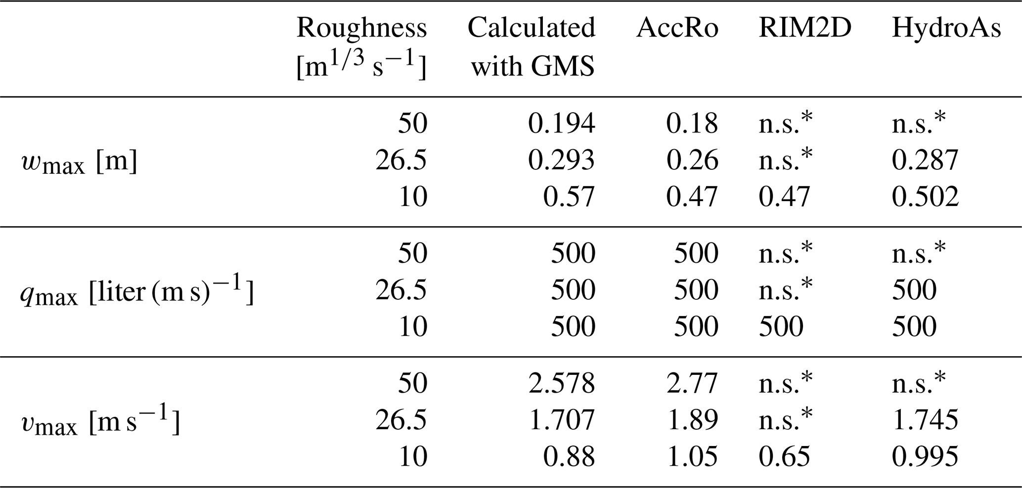
^* Simulation did not stabilize.

For the real-world scenario, we used the catchment Riedgraben, which is located in south-western Germany. The catchment area is approximately 3 km² , of which 0.67 km² is urban (Bretten–Diedelsheim) and the rest is divided into agricultural and forest areas. The assigned roughness values based on the land use are shown in Fig. 6c. The hydrological input s was calculated with the model RoGeR (Steinbrich et al., 2016) for an observed extreme rainfall event as well as for three design events. These were defined based on the 1 h extreme rainfall event with a return period of 30 and 100 years and defined probable maximum precipitation PMP for this area (LUBW, 2016) (Table 1). The spatial and temporal distributed runoff intensities were then used as input into the three different models. The spatial resolution for RIM2D and AccRo was set to 2 × 2 m². The DEM and hydraulic roughness were obtained from the TIN data used by HydroAs. HydroAs results were rasterized with the ha2raster tool (Hydrotec, 2025) so that a one-to-one comparison of the three models was possible. The focus of the evaluation was on the spatial pattern of maximum water depth, maximum specific discharge and maximum flow velocity.

3 Results

3.1 Steady-state simulations

Tables 2 and 3 show a comparison of the Gauckler-Manning-Strickler (GMS) solutions and the three model results. To avoid boundary effects, the values were taken at the centre of the row 10 m above the end of the hillslope or channel. For the steady-state situation of the hillslope scenario (Table 2), AccRo and HydroAs match the expected values, independent of the roughness conditions. RIM2D results were only stable for the high roughness values, and lateral dispersion seems to be rather large in RIM2D (see Fig. 7a). This and the fact that some water is already lost through the left/right boundaries before reaching the bottom of the slope leads to a lower water depth in the middle of the hillslope. Therefore, RIM2D underestimated w_max, q_max and v_max.

For the channel scenario (Table 3), HydroAs results are slightly closer to the expected values than the values of AccRo for roughness values of 10 and 26.5 m${}^{\mathrm{1}/\mathrm{3}}$ s⁻¹. Here water depths of AccRo are less than expected. As mentioned before, AccRo calculates w_max and v_max without any knowledge of a structure like channel width (i.e. 2 m or 2 cells). Instead of using the “real” hydraulic radius, it uses water depth (see Sect. 2.1.2). The specific discharge of 0.5 m³ (s ⋅ m)⁻¹ (1 m³ s⁻¹ distributed in a 2 m wide channel) is equal to the GMS results. RIM2D results are again only stable for the high roughness values. w_max of RIM2D is equal to AccRo, but v_max of RIM2D is lower than v_max of the other two models.

The finding that for some combinations we could not stabilize the simulations of the 2d hydrodynamic models (mainly RIM2D, but in one case also HydroAs) demonstrates that the AccRo method which is based on iterations and not on model internal computation time steps provides numerically rather robust results. This allows to also apply AccRo for more complex cases that require a relatively fine spatial resolution.

Additionally, note that for RIM2D the relation $q=w\cdot v$ is not fulfilled under stationary conditions, since v in RIM2D is a secondary variable only, while q and w are numerically calculated.

Figure 7a compares the cross-sectional values of the inundation depth along the hillslope case for a roughness of 10 m${}^{\mathrm{1}/\mathrm{3}}$ s⁻¹. The inundation depth in the middle of the hillslope (x= 500 m) is equal to the values in Table 2 for HydroAs and AccRo.

Figure 7 Cross section of inundation depths at top of the hillslope (2 m) and after 1500 m of the hillslope scenario under stationary conditions (a). Cross section of the channel scenario at 1500 m (b) showing the DEM plus inundation depth.

In any case, comparing the input's dispersion downslope reveals that the 500 m wide rectangular input spreads along the flow path. The inundation depth of HydroAs and AccRo remains equal in the middle of the hillslope, and the spatial extension downward is comparable. After 1500 m, the inundated area extended on both sides by approximately 100 m for HydroAs and 120 m for AccRo. The RIM2D dispersion is much more pronounced, and after 1500 m flow distance, the inundated area reaches the limits of the hillslope. Actually, RIM2D hits the left and right boundaries after around 1040 m, but the other models do not reach them until 2000 m. Figure 7b depicts the cross section of the channel after 1500 m. As shown in Table 3, the water depths of AccRo and RIM2D are equal, while HydroAs simulates slightly higher water depths.

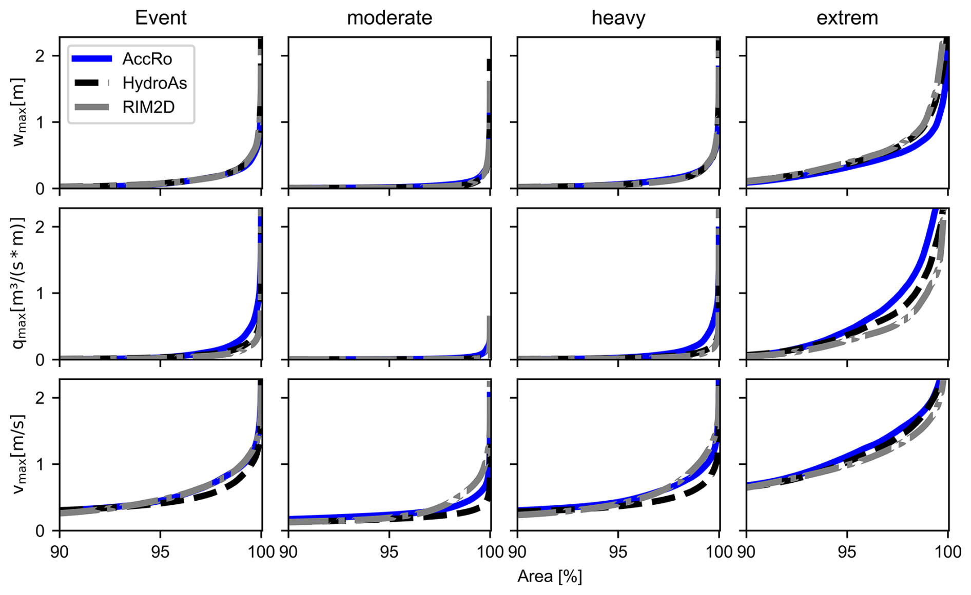
Figure 8 Comparison of the exceedance probability distribution of w_max, q_max and v_max for the four different s.

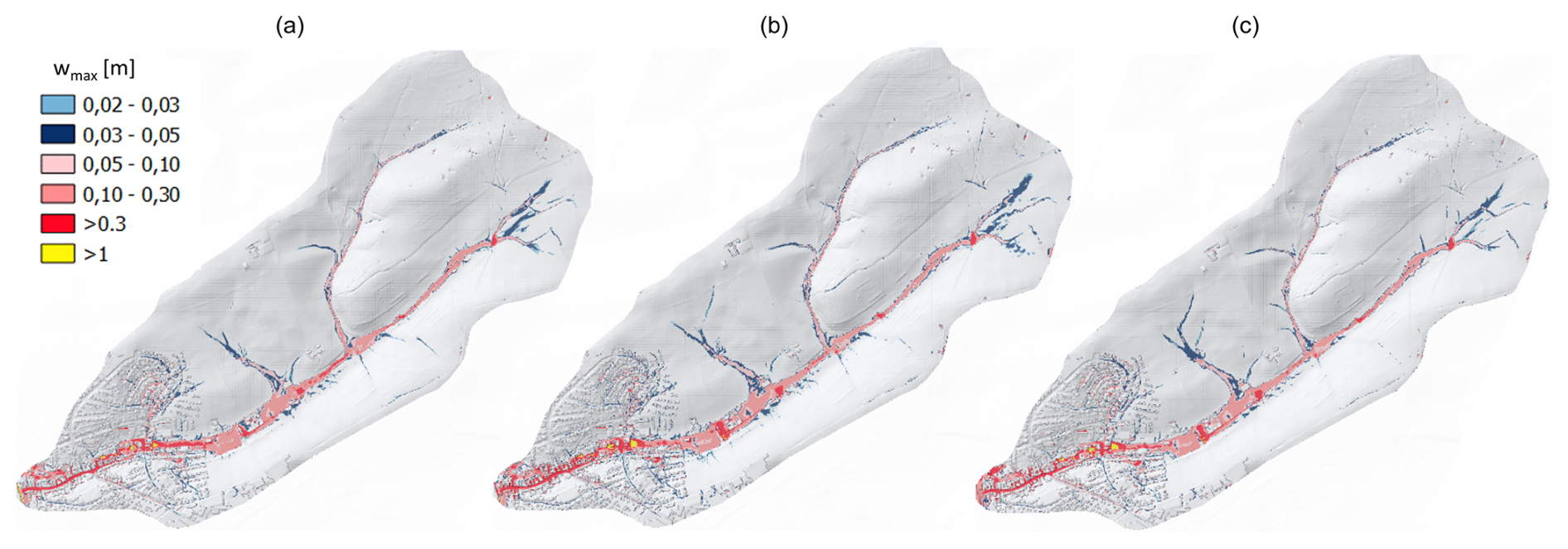
Figure 9 Visual comparison of w_max for s input “event” as simulated by AccRo (a), HydroAs (b) and RIM2D (c).

3.2 Catchment simulations

The simulations of the real catchment differ from the scenarios described in Sect. 3.1 due to temporal and spatial non-stationary input and due to a much more complex hydraulic situation. We evaluate and compare the three target values w_max, q_max and v_max in three ways: their distributions to evaluate the overall probabilities of exceedance without spatial explicit comparisons, visually through maps and direct grid-cell to grid-cell comparison, including the slope of a linear regression and the correlation coefficient. In addition, we compare the hydrographs of the hydraulic models to those generated using the GIUH approach.

In Fig. 8 the exceedance probability distributions of catchment area with w_max, q_max and v_max (rows) are shown for the 4 different events (columns). To highlight the most relevant inundation area, only the upper 10 % is shown. For all variables and cases, the 3 models show rather similar results. Only for the extreme design event (PMP) does AccRo have slightly higher q_max and v_max values and slightly lower w_max values than the other two hydraulic models. The high agreement between the three models' results is also visible in the spatial patterns of inundation depth for the observed event (see Figs. 9 and S1 to S3 in the Supplement for other parameters and cases), where all three methods provide extremely similar spatial patterns of maximum inundation depths, particularly for the observed event.

To assess a stricter metric, we examined the simulation results of the three models for the parameters w_max, q_max and v_max for all four cases on a grid-cell by grid-cell basis (see Fig. 10 for the observed event and the supplemental materials for the three other scenarios). For w_max (Fig. 10, upper row), AccRo matches the two hydraulic models very well, with the vast majority of cells plotting close to the one-to-one line and only a slight tendency for underestimating the inundation depth. For q_max and v_max, AccRo generally simulates larger values than HydroAs and RIM2D, which is most pronounced in the case of q_max (Fig. 10, central row). However, the correlation between the two hydraulic models is not as strong for q_max and v_max as it is for w_max. Especially for v_max, RIM2D appears to have significantly slower maximum flow velocities than HydroAs (Fig. 10, bottom row), which is in the same order of magnitude as the differences between AccRo and the hydraulic models. If we apply the same analysis for the 3 scenarios (see Figs. S1 to S3), we find the same patterns as for the observed event case. In general, AccRo and HydroAs agree more closely either does with RIM2D.

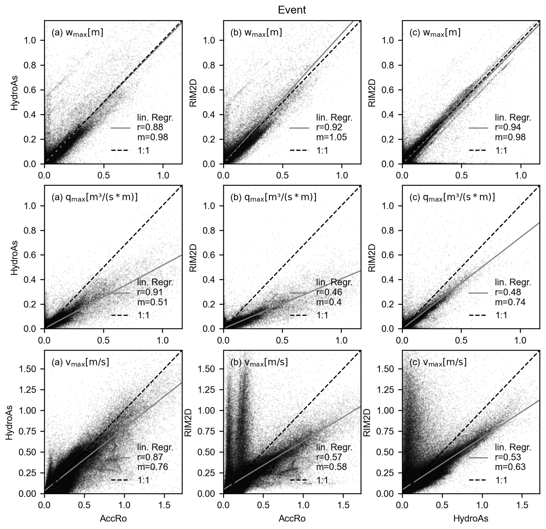
Figure 10 Scatterplot of the three models. First row w_max (m), second row q_max (m³ (m ⋅ s)⁻¹) and third row v_max (m s⁻¹) for the real event. In addition, the linear regression (grey) and 1:1 line (dashed black) as well as the slope of the linear regression (m) and the Pearson correlation coefficient (r) are shown.

Figure 11 shows the hydrographs for the four events. Compared to the hydraulic models, the hydrographs at the catchment outlet of AccRo show an earlier rise and faster drop. With respect to the peak time difference, all simulations are within 2 min in the case of the observed event, but show larger deviations for the three scenarios (see Table S1). The overall response and total discharge are always lower for the hydraulic models, most likely because the simulations of the hydraulic models are stopped before the catchment is completely dry and they also typically retain some water in the catchment as the flow velocities decrease for very low inundation depths. Under more extreme conditions (event and extreme case), the three models produce more similar hydrograph responses.

Figure 11 Hydrographs at the catchment outlet for the four simulated events.

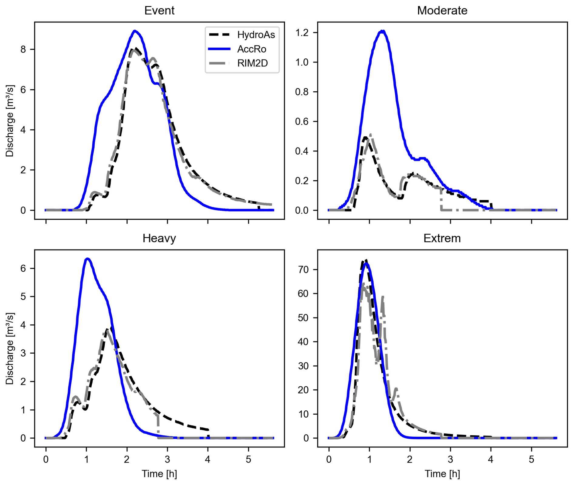
This finding is also supported when calculating quantitative performance metrics. In case of the observed event, the mean absolute error ranges from 1.25 m³ s⁻¹ (AccRo and HydroAs) to 1.51 m³ s⁻¹ (AccRo and RIM2D) compared to 0.23 m³ s⁻¹ for the two hydrodynamic models. For the same case the peak percentage difference range from 9 % (AccRo and HydroAs) to 11 % (AccRo and RIM2D) compared to 2 % for the two 2d hydrodynamic models. For the three scenario simulations the deviation between AccRo and the two hydrodynamic models is sometimes larger, however, also the agreement between the hydrodynamic models themselves is generally lower (see Tables S2 and S3 for all cases).

4 Discussion

The validation experiment shows that for the design cases, AccRo is able to reproduce the “hard facts” of the analytical solutions. For the real world case, however, hard facts are not available, since there is neither a database of systematically observed inundation areas available nor analytical solutions producible. Hence, we use the output of two state-of-the art hydrodynamic models as reference cases, acknowledging that differences in the outcome of the different methods could be attributed to both shortcomings in AccRo and shortcomings in the hydrodynamic models. Hence, we do not aim for a perfect match of AccRo and the hydrodynamic models, but rather at a “realistic” outcome of AccRo. Still future work should seek opportunities to evaluate AccRo against measured flood data in order to further enhance the confidence in the outcome of AccRo.

Given the results for the event and scenario simulations for the Riedgraben catchment we see that AccRo tends to have higher q amounts then the hydrodynamic models. In AccRo this value depends on the one hand on the accumulated surface runoff as well as the empirically derived function F. F represents a combination of area specific (DEM and roughness) and event (surface runoff response) specific characteristics. The latter takes account of the fact that for the same precipitation amounts, different areas generate different runoff but also that the same area can react differently due to different preconditions, such as moisture conditions. Investigating the behaviour of F for different types of events we find that F indeed is varying quite substantially (not shown), however it becomes evident that after a specific t_b (twice the duration of the event), the values for F are converging.

In the case of the two hydrodynamic models, maximum specific discharge is calculated as the temporal maximum of the product of w and v at each time step, which means that it accumulates potential errors in both variables and therefore might be not so robust than the individual parameters. Given the fact that w is rather similar in all three models, also enhances the confidence in the q_max output of AccRo, since in AccRo w_max is directly calculated from q_max. Differences in v_max are mainly obvious when compared to RIM2D and for the case of the hydrograph. While v_max in RIM2D is known to be generally to slow, due to the inclusion of a numerical diffusion term to enhance model stability (Bates et al., 2010), the fast buildup and decrease of the hydrograph peak in AccRo is immanent, since max w_max is used to calculate forward flow time (t_f) for each raster cell through the entire runoff event.

Like every model AccRo is based on a series of assumptions and empirical approaches, not all to be justifiable by hand. Examples for these are e.g. the approach to estimate the ideal number of iterations or exact size and definition of the area F is representative for. A major advantage of AccRo, when compared to the hydrodynamic models, however, is the numerical stability of the approach since it is independent of a model's internal time step (see the design test cases, where both hydrodynamic models had stability issues). This is also beneficial when it comes to computational efficiency. On top of the number of grid boxes, computation time in AccRo mainly depends on the number of iterations, while in hydrodynamic models the duration of the event – and more importantly – the adaptation of the model's internal time step to the horizontal resolution or to stability criteria is required. For the test case of the Riedgraben (∼ 0.75 million grid boxes), AccRo and RIM2D both simulated the observed event in less than 2 min (real time) what is fast if compared to HydroAs simulation time of ca. 2 h. However, AccRo and HydroAs were running on standard CPUs, whereas RIM was iterated on a high-efficiency GPU. For a detailed overview on the computation times for each of the four simulations conducted in the Riedgraben catchment as well as the used computing systems see Table S4. The downside of using iteration instead of internal model time steps in AccRo is, that AccRo only can model the maximum states of w, q, and v and not the temporal evolution of these variables.

In the light of using AccRo as a tool for the generation of local pluvial flood maps or real-time inundation forecasting, it certainly would be beneficial to include processes into the model so far not tackled. Especially the representation of the capacity of culverts or road passages would be aspects that should be tackled when further developing AccRo. In this turn, also focusing on computational efficiency and parallelization would increase the suitability of AccRo for forecasting even further.

5 Conclusions

In conclusion, this paper describes an alternative method to hydraulic models to derive critical variables w_max, q_max and v_max caused by pluvial flooding. The comparison with analytical solutions and hydraulic models shows good agreement. Given this finding and keeping in mind its computational efficiency demonstrates the suitability of AccRo for operational use cases. Still AccRo has some limitations. In addition to the process still missing, AccRo cannot show the temporal development of the variables and hence does not simulate flood timing and dynamics. So a meaningful application of AccRo depends on the issue. When the focus lies on estimating flood hazards on the basis of maximum inundation depths, maximum flow velocities or maximum specific discharge, AccRo is very valuable tool.

With the use of the GIUH method, the temporal aspect can be included in the simulation, but the assumption of a constant velocity for one cell over the entire runoff event is not realistic. So here again, if the focus of the simulation is mainly the height of peak discharge, it might be justified to use AccRo. Otherwise a hydraulic simulation should be preferred.

Appendix A: List of variables.

Variable name	Description
AA	Area weighted Flow
	Accumulation (L2)
$A_{{\mathrm{A}}_{\mathrm{crit}}}$	Constant (critical accumulation
	= 10.000 m2 )
As	Runoff weighted Flow
	Accumulation (L)
C	Cross sectional area of flow [L2]
DEM	Digital Elevation Model [L]
F	Factor to transfer As to q [1 T−1]
i	Slope [L/L]
k	Strickler coefficient for
	determining surface roughness
	[L${}^{\mathrm{1}/\mathrm{3}}$ T−1]
l	Cell size [L]
L, T	Dimensions Length, Time
p	Precipitation rate [L T−1]
Q	Discharge [L3 T−1]
q	Specific discharge [L3 (T ⋅ L)−1]
R	Hydraulic radius [L]
s	Surface runoff intensity [L T−1]
$s_{\max },w_{\max },q_{\max },v_{\max }$	Represents maximum value of
	parameters
Sr	Sinks [L]
tb	Backward flow time [T]. Overall
	duration of flow through a cell
	caused by transit times from
	upslope cells [T]
tc	Flow time of a cell based on flow
	velocity [T]
v	Flow velocity [L T−1]
w	Inundation depth [L]
wr	Water depth above roughness is
	independent of w [L]
wsf	Upper limit of water depth for
	sheet flow [L]