Assessing seasonal climate predictability using a deep learning application: NN4CAST

Seasonal climate predictions are essential for climate services, with changes in tropical sea surface temperature (SST) representing the most influential oceanic drivers. SST anomalies can affect the climate in remote regions through various atmospheric teleconnection mechanisms, and the persistence/evolution of those SST anomalies can give seasonal predictability to atmospheric signals. Dynamical models often struggle with biases and low signal-to-noise ratios, making statistical methods a valuable alternative. Deep learning models are currently providing accurate predictions, mainly in short-range weather forecasts. Nevertheless, the black-box nature of this methodology makes it necessary to ensure its explainability. In this context, we present NN4CAST (Neural Network foreCAST), a Python deep learning pipeline designed to assess seasonal predictability, with built-in tools for evaluating model skill and performing basic spatial diagnostics based on empirical orthogonal functions. Starting from the raw datasets, NN4CAST performs all methodological steps: preprocessing, training and evaluation, enabling researchers to rapidly explore the predictability of a target variable and identify its main potential drivers. This flexible framework allows for the quick testing of predictive skill from different sources of predictability, making it a valuable asset for climate services. Although NN4CAST can use different variables to feed the model, we illustrate its application to reproduce tropical and extratropical teleconnections by training the model with Pacific SST anomalies. We show that NN4CAST can provide skilful predictions across timescales, from modelling variables at lag 0 that capture observed relationships to producing seasonal forecasts at longer leads, both in regions with linear SST-atmosphere coupling (tropics) and in highly non-linear remote regions (such as Europe). Two key examples are the prediction of SST anomalies in the tropical Atlantic region during boreal spring from previous winter SSTs, and the modelling of precipitation anomalies over the European continent in boreal fall from the contemporaneous Pacific SSTs. The former exemplifies a predominantly linear ENSO-Tropical North Atlantic teleconnection, whereas the latter involves a highly non-linear and non-stationary ENSO-Euro-Atlantic teleconnection. Our results demonstrates NN4CAST's potential to determine and quantify the influence of specific potential drivers on a target variable, offering a useful tool for improving climate predictability assessments. NN4CAST enables the attribution of predictions to specific input features, helping to identify the relative importance of different sources of predictability over time and space. In summary, NN4CAST offers a powerful framework to better characterize and understand the complex, non-linear and non-stationary remote climate interactions.

1 Introduction

Seasonal forecasting attempts to provide useful information about the climate that can be expected from 1 up to 12 months. It is crucial for different sectors such as agriculture, water resource management or disaster preparedness. Seasonal predictions are mainly justified by the existence of interactions between the atmosphere and the slow, and predictable, variations in some of the components of the climate system, such as soil moisture, snow cover, stratospheric circulation, ocean heat content or sea surface temperatures (SSTs). Specifically, tropical SSTs are demonstrated to be one of the most important sources of predictability at seasonal timescales due to its characteristic persistence and evolution (Shuila and Kinter, 2006; Kirtman and Pirani, 2009; Ineson and Scaife, 2009). Earth system models (ESMs) simulate the climate system by solving the mathematical equations that represent the interactions between its components. However, they have errors due to not only the numerical resolution of the system of equations, but also to the uncertainty in the initial and boundary conditions (Hargreaves, 2010). Within the context of seasonal timescales, different challenges, whether occurring independently or in combination, may arise. For example:

1. Seasonal prediction skill relies on the correct representation of both local processes, such as deep convection, and large-scale ones, such as global teleconnections. A misrepresentation of either of them leads to poor performance in certain remote regions, where the interaction of the different signals is non-linear and seasonally dependent (Gleckler et al., 2008; Doblas-Reyes et al., 2013).

2. Oceanic patterns of variability, which may provide seasonal predictability in certain regions such as the Atlantic Niño or the North-Atlantic SSTs, are not well represented by current models (Richter and Tokinaga, 2020; Roberts et al., 2021).

3. Multidecadal ocean variability and the global warming trend alter the global circulation and, consequently, the way in which atmospheric teleconnections (i.e., Rossby waves forced by El Niño) propagate, thereby introducing non-stationarities into the system (López-Parages et al., 2015; Weisheimer et al., 2017). ESMs exhibit mean state biases and struggle to represent interannual-to-decadal variability, failing to reproduce these non-stationarities. Statistical models appear as an alternative to overcome these limitations.

4. The generation of coupled dynamical simulations at these timescales demands substantial computational resources which, in turn, constrains the potential for enhancement in spatial resolution (Doblas-Reyes et al., 2013).

As an alternative to ESMs, statistical methods directly focus on the patterns and relationships between different climate variables with multiple time lags (Wilks, 2011). Another key advantage is their high computational efficiency, as they require significant computing power only during the training phase. Artificial Intelligence (AI) encompasses computational methods that enable machines to learn from data and make predictions (Russell and Norvig, 2016). Within AI, Machine Learning (ML) develops algorithms that identify patterns and generalize to new situations (Samuel, 1959). Deep Learning (DL), a subset of ML using neural networks with multiple hidden layers, excels at capturing complex, high-dimensional relationships without manual feature engineering. Convolutional Neural Networks (CNNs), a widely used DL architecture, learn spatial hierarchies in the data, making them particularly effective for climate applications (LeCun et al., 2015; Rawat and Wang, 2017). The potential of DL for climate prediction is evident in the growing number of models developed from empirical data rather than explicit physical equations. Recent examples include PanguWeather (Huawei Cloud Group), GraphCast and NeuralGCM (DeepMind and Google) (Bi et al., 2023; Lam et al., 2023; Kochkov et al., 2024), which generate sub-daily forecasts of the Earth system in an autoregressive manner.

The application of deep learning models to seasonal forecasting and the evaluation of teleconnections remains relatively scarce. Other ML techniques such as linear regression, principal component analysis, correlation, and maximum covariance analysis have been widely applied with satisfactory results (Wilks, 2014; Suárez-Moreno and Rodríguez-Fonseca, 2015; Rieger et al., 2021). Despite this, DL offers the potential to overcome current limitations by improving forecast accuracy and enabling analysis of the underlying attribution mechanisms. Existing DL studies have typically targeted individual phenomena, such as El Niño–Southern Oscillation or the Atlantic Niño (Ham et al., 2019; Shin et al., 2022; Bachèlery et al., 2025). However, those approaches produce tailored models for each case, without built-in explainability or generalizability to other teleconnections.

For these reasons, we have developed the Neural Network foreCAST (NN4CAST) application, a Python library designed to facilitate the creation of simple deep learning models for reproducing climate teleconnections driven by different sources of seasonal predictability. NN4CAST provides a flexible framework for non-linear statistical analysis, allowing researchers to efficiently quantify the predictive skill of various sources of predictability. Our approach, in contrast to other ML-based models, facilitates the development of a user-friendly model characterized by a simple architecture and low computational cost. The NN4CAST framework is designed to mitigate the risk of treating DL models as “black boxes”, facilitating the interpretation of predictability sources and allowing the assessment of sensitivities to the training period and/or predictor domain. While these capabilities are intrinsic to the framework, the present work focuses on model skill and attribution patterns. This interpretability represents an important added value of NN4CAST compared to other DL seasonal forecasting models (Pan et al., 2022; Watt-Meyer et al., 2024), and is consistent with recent demonstrations that ML weather models trained on reanalysis can yield skilful seasonal predictions while posing interpretability challenges that call for simpler and more transparent experimental setups (Kent et al., 2025). It enables the analysis of predictability, as well as the examination of teleconnections, their modulations, the identification of windows of opportunity and the production of attributions of the predictions over certain target regions. NN4CAST is implemented as a Python library intended for use in applications with small or large datasets for seasonal or decadal predictions. Scientific tools are commonly written using low-level compiled languages such as C or C$++$ (such as the Climate Data Operators, CDO, Schulzweida et al., 2019), due to their greater computational efficiency compared to high-level interpreted languages such as Python. However, Python has become the dominant programming language for ML tools, including the libraries used in NN4CAST.

This paper introduces the NN4CAST package, outlining the theoretical foundations of neural networks and detailing its core features. We focus on two well-known climate teleconnections: the Tropical North Atlantic (TNA) SST and European precipitation patterns, which are influenced by Pacific SST anomalies. While these teleconnections are broadly recognized in the literature, the potential of SST to enhance seasonal forecasts has not been fully assessed (Alexander et al., 2002; López-Parages and Rodríguez-Fonseca, 2012). Moreover, the NN4CAST framework extends beyond ocean variables, enabling the investigation of predictability in additional climate components such as soil moisture, snow cover or sea ice. The remainder of the paper is organized as follows: Sect. 2 reviews fundamental concepts in DL; Sect. 3 describes the NN4CAST methodology and implementation; Sect. 4 presents illustrative applications and evaluates performance; and Sect. 5 summarizes the main conclusions and outlines directions for future work.

2 Theoretical framework

Seasonal prediction systems typically use a predictor field X initialized at time t₀ to forecast a predictand field Y at t₀+τ, taking advantage of the persistence of climate anomalies in X. NN4CAST generalizes this setup by enabling the analysis of statistical relationships between X and Y at any temporal lag, from contemporaneous (τ=0) to predictive configurations (τ>0). Considering τ=0 does not imply causality, but rather functional relationships, which are crucial for understanding teleconnections. Although numerous statistical methods exist for seasonal prediction, the present work adopts a DL framework. Construction of the neural network entails the selection of hyperparameters, such as network depth, layer widths, activation functions, optimization algorithm and regularization strategies (Géron, 2022). Training is performed by minimizing the Mean Squared Error (MSE) loss, defined as:

$$\begin{array}{}\text{(1)}& \mathrm{MSE}={\displaystyle \frac{\mathrm{1}}{m}}\sum _{i=\mathrm{1}}^m{\left(y^{\left(i\right)}-{\widehat{\mathbf{y}}}^{\left(i\right)}\right)}^{\mathrm{2}}\end{array}$$

where m is the number of samples in the dataset, ${\widehat{\mathbf{y}}}^{\left(i\right)}$ is the predicted value of the predictand variable for the ith instance in the dataset and y⁽ⁱ⁾ is its corresponding real value (i.e., the ground truth) (Wilks, 2011). However, it is possible to modify this objective function to any other differentiable loss function (Cuomo et al., 2022). After training by minimizing the loss function, the model parameters are fixed and used to generate forecasts on the independent test set. Forecast skill is then quantified using the Root Mean Squared Error (RMSE), defined as the square root of the MSE and the Anomaly Correlation Coefficient (ACC), which is given by:

$$\begin{array}{}\text{(2)}& \mathrm{ACC}={\displaystyle \frac{\sum _{i=\mathrm{1}}^m{y}^{\left(i\right)}{\widehat{y}}^{\left(i\right)}}{\sqrt{\sum _{i=\mathrm{1}}^m{\left(y^{\left(i\right)}\right)}^{\mathrm{2}}}\sqrt{\sum _{i=\mathrm{1}}^m{\left({\widehat{y}}^{\left(i\right)}\right)}^{\mathrm{2}}}}}\end{array}$$

where ${\widehat{\mathbf{y}}}^{\left(i\right)}$ is the predicted anomaly of the predictand variable for the ith instance in the dataset, and y⁽ⁱ⁾ is its corresponding observed anomaly, both computed relative to the same climatology (Wilks, 2008).

To achieve a more robust and unbiased evaluation of model performance, NN4CAST implements a cross-validation approach wherein the dataset is systematically partitioned into training and testing subsets across k folds. This iterative process ensures that each sample is utilized for both training and validation, thereby maximizing the use of available data and providing a comprehensive assessment of the model's generalization capabilities. Furthermore, NN4CAST offers the option to perform leave-one-out cross-validation (k = number of samples in the dataset), where each individual sample is used once as a test set while the remaining samples form the training set. This method yields a detailed skill assessment across the entire dataset, facilitating the construction of a full-period hindcast and enhancing the reliability of predictive evaluations (Michaelsen, 1987).

To facilitate a comprehensive analysis of the mechanisms driving the predictions, eXplainable AI (XAI) techniques are employed to assess the relative importance of predictor field features for a given region of the predictand field. XAI aims to enhance the interpretability of AI methods by identifying the most influential predictor areas in the prediction process. Two main categories of methods exist: sensitivity methods, which assess how changes in a specific predictor affect the output, and attribution methods, which determine the relative contribution of each predictor to the predictand (Guidotti et al., 2018). In this work, we employ one of the most widely used attribution methods, Integrated Gradients (IG), which provides theoretically grounded feature attributions that satisfy desirable axioms such as sensitivity and implementation invariance (Sundararajan et al., 2017). IG is particularly suitable for high-dimensional and complex predictor fields, typical of climate data, as it quantifies the contribution of each input relative to a chosen baseline reference vector $\widehat{\mathit{x}}$, for which the model output is zero: $\widehat{\mathit{F}}\left(\widehat{\mathit{x}}\right)=\mathrm{0}$. The importance is computed as the product of the distance between the input within the reference point, and the average of the gradients at points along the straight-line path from the reference point to the input feature. Specifically, the mathematical expression is given by:

$$\begin{array}{}\text{(3)}& R_{i,n}=\left(x_{i,n}-{\widehat{\mathit{x}}}_i\right){\displaystyle \frac{\mathrm{1}}{m}}\sum _{j=\mathrm{1}}^m{\displaystyle \frac{\partial \widehat{\mathit{F}}}{\partial X_i}}{|}_{X_i={\widehat{\mathit{x}}}_i}+{\displaystyle \frac{j}{m}}\left(x_{i,n}-{\widehat{\mathit{x}}}_i\right)\end{array}$$

where X_i are the input features, R_i,n the relevance of feature at grid point (i) for the model prediction of sample (n), $\widehat{\mathit{F}}$ the function learned by the model and (m) the number of steps in the Riemann approximation (Mamalakis et al., 2022). The attributions computed using this equation provide a quantification of the contribution of each input feature to the predicted output for a given target region. By integrating gradients along the path from a baseline input to the actual predictor field, we can identify the most influential regions and quantify their relative importance. These attributions reflect statistical associations captured by the model and should not be interpreted as evidence of direct causal relationships. This approach allows the model to remain entirely data-driven, while providing interpretable information at the feature level on the factors that determine seasonal predictability, in line with XAI principles. The next section describes how this theoretical framework is implemented in the NN4CAST tool.

3 NN4CAST methodology and implementation

Building on the key elements of the DL methodology outlined above, the NN4CAST library integrates these approaches into a unified framework. The whole procedural workflow is depicted in Fig. 1:

• Preprocessing of the datasets according to user targets, including: data loading, selection of the region and season of interest, anomaly computation, and trend removal (I in Fig. 1).

• Construction of a deep neural network for seasonal prediction, with training performed through the minimization of the MSE (II in Fig. 1).

• Application of regularization techniques to mitigate overfitting (II in Fig. 1).

• Model performance evaluation using cross-validation strategies, employing different skill metrics (RMSE and ACC, II in Fig. 1).

• Attribution analysis within the XAI framework to identify the contribution of different regions of the predictor field to the model predictions (III in Fig. 1).

• Empirical Orthogonal Function (EOF) analysis of model outputs and observational data to compare dominant modes of variability and assess the physical consistency of predictions (III in Fig. 1).

• Optimization of model hyperparameters to improve generalization and predictive performance (IV in Fig. 1).

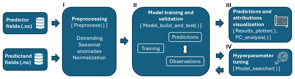
Figure 1 Flowchart illustrating the methodology and application workflow of the NN4CAST library, designed for processing monthly data and assessing seasonal climate predictability. The Python function names corresponding to each step are shown in brackets.

Each of the above mentioned steps is computed by the application of different Python functions designed within NN4CAST (Fig. 1). The application begins by loading predictor and predictand datasets and defining model hyperparameters. A standardized preprocessing pipeline is then applied via the Preprocess() function. Next, the model is built, trained, and tested using Model_build_and_test(), which integrates attribution routines to compute feature importance maps for each forecast. Once training is complete, Results_plotter() visualizes both the individual predictions and their associated attribution maps, making the physical drivers of skill explicit. Optionally, Model_searcher() can be used to optimize performance through hyperparameter tuning, and PC_analysis() enables EOF analysis of model outputs versus observations to assess dominant spatial modes of variability. Finally, the entire workflow can be configured via the main module nn4cast.predefined_classes.

The principal distinguishing feature of NN4CAST lies in its design, which specifically targets the assessment of teleconnection predictability, enabling experiments to address common challenges in seasonal climate forecasting. While some of these challenges could be partially addressed by simpler models, NN4CAST leverages deep learning to capture complex, nonlinear relationships and spatial interactions that are often missed by linear approaches. The main challenges in seasonal climate forecasting, discussed in the introduction, are tackled by NN4CAST through the following strategies:

1. Representing teleconnection drivers at interannual timescales. The models created by NN4CAST can capture nonlinear and spatially distributed interactions among predictors across different regions, enabling a more accurate assessment of each region contribution to the predictand.

2. Non-stationarity of climate relationships. The models created by NN4CAST can be trained over different periods, enabling the analysis of how predictor-predictand relationships evolve over time.

3. Computational efficiency. The models created by NN4CAST are optimized to perform simulations within minutes on a standard computer, despite modelling high-dimensional and complex predictor fields.

4. Interpretability of DL models. The models created by NN4CAST provide feature attributions that reveal the main drivers and underlying physical mechanisms of predictions, combining the flexibility of DL with interpretability.

3.1 Configuration of hyperparameters and preprocessing

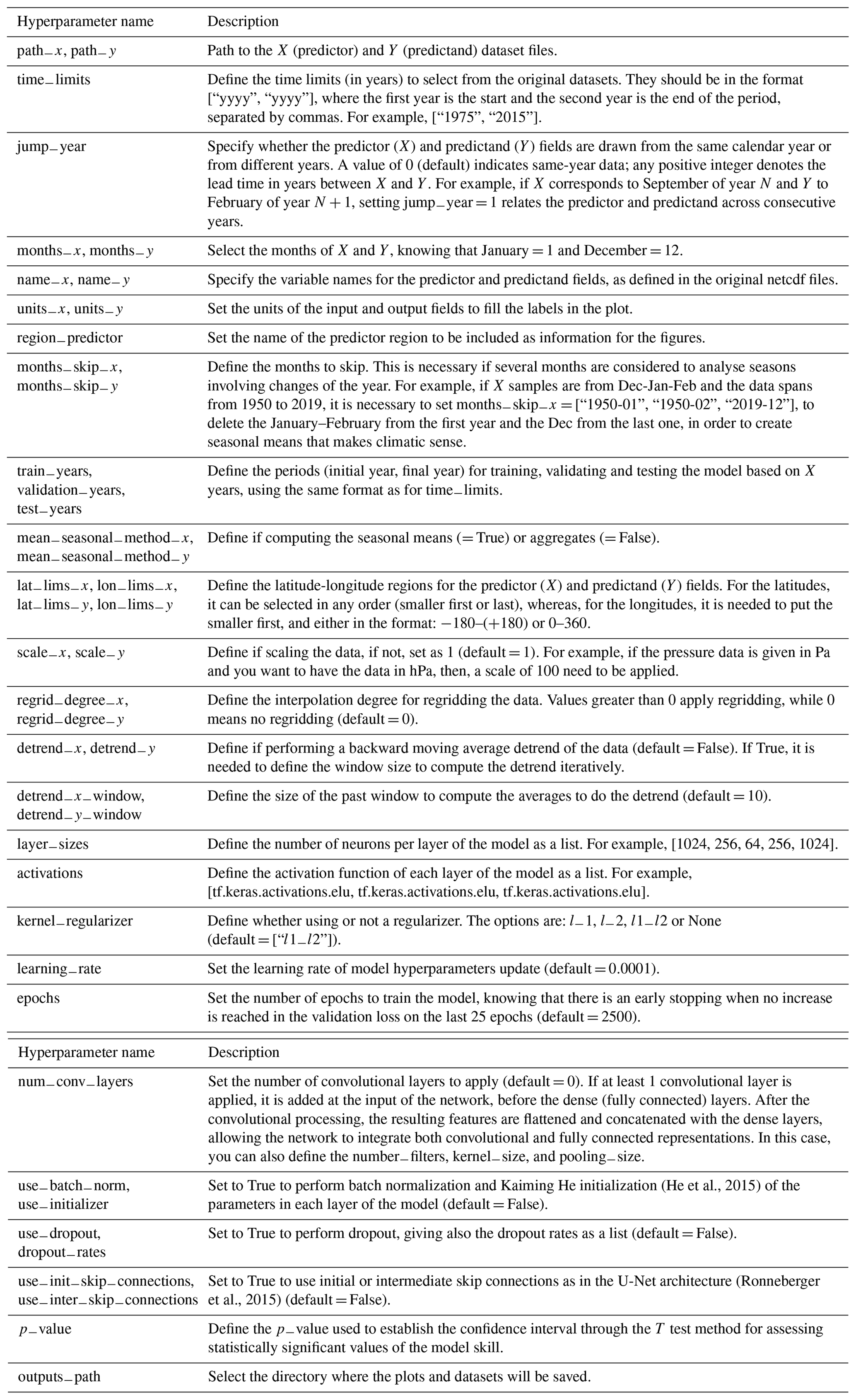
NN4CAST employs datasets stored in the netCDF4 format (Rew et al., 2006), a widely used standard within Earth data science. These datasets are structured as space-time matrices and require three coordinates: time, latitude, and longitude. As NN4CAST is designed for seasonal timescales, the time coordinate must be defined at a monthly resolution. The hyperparameters required by the application are summarized in Table 1, including a brief description of their functionality. These hyperparameters are stored in a dictionary that can be saved as a YAML file to document the experiment setup for easy retrieval and reproducibility. The next step involves preprocessing the predictor and predictand data according to the operations specified in the hyperparameter dictionary, such as regridding, computing seasonal means, and detrending. Detrending is performed using a backward moving average (BMA) algorithm, which computes the running mean of previous years using a sliding window and subtracts it from subsequent values (Raffalovich, 1994; Alvarez-Ramirez et al., 2005). This approach ensures that future information is not introduced during preprocessing. For a complete description of the code implementation, including the creation of the hyperparameter dictionary and the preprocessing workflow, the reader is referred to the Supplement (Listings S1–S3).

(He et al., 2015)(Ronneberger et al., 2015)

Table 1 Table listing the names and detailed descriptions of the hyperparameters used in the NN4CAST application, which govern the model configuration and training process. Default values have been optimized for various climate variability studies using the built-in hyperparameter optimization function Model-searcher. These defaults provide reliable performance, although some hyperparameters can be adjusted depending on the specific dataset or application.

3.2 Layer-by-layer specification of the default architecture

To ensure full reproducibility, we provide a layer-by-layer description of the default architecture used in the Pacific–European teleconnection experiment (Sect. 4.2), corresponding to the hyperparameter configuration in Table 3. For this configuration, num_conv_layers=0 and no skip connections are used; thus, the model reduces to a fully connected encoder–decoder network. If convolutional layers were included, they would use two-dimensional convolutions with unit stride and same padding, preserving the spatial dimensions. For an input tensor of size (H, W), the output would retain the same spatial resolution, (H, W), while the channel dimension would become equal to the number of filters F, yielding a tensor of shape (H, W, F). After flattening, this corresponds to a vector of size $H\times W\times F$. For each hidden dense layer, the following sequence of operations is applied: Dense → Batch Normalization → ELU activation. Batch normalization, kernel regularizer and dropout are included only when use_batch_norm=True, use_initializer=True and use_dropout=True, respectively. When enabled, kernel regularization and dropout are applied immediately after the flattening layer. In the present configuration, a dropout rate of 0.1 is used. The output layer employs a linear activation function and does not include dropout. The resulting output vector is reshaped to the predictand field size. Model parameters are optimized by minimizing the mean squared error (MSE) using the Adam optimizer with a learning rate of 10⁻⁴. A schematic representation of the architecture is shown in Fig. 2.

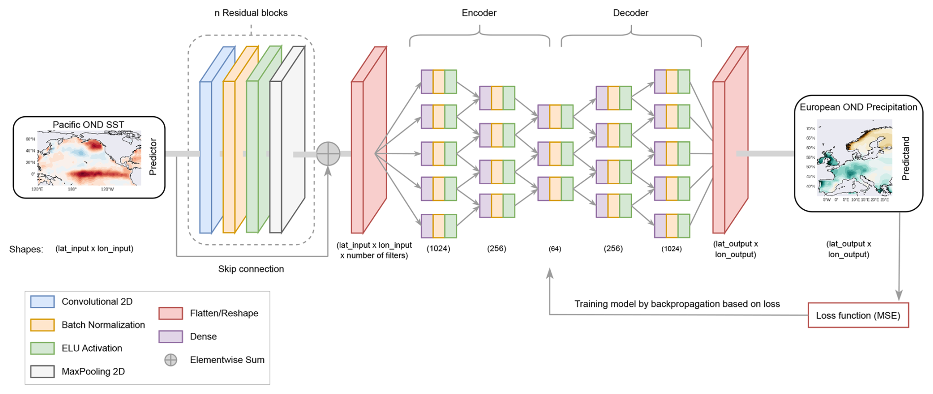
Figure 2 Schematic of the NN4CAST model architecture used in this study to analyse the predictability of the Pacific-European precipitation teleconnection (Sect. 4.2). The network consists of an initial block of convolutional layers (if the hyperparameter num₋conv₋layers is set to a value different from 0), followed by several fully connected (dense) layers, whose number and size are defined by the hyperparameter layer₋sizes (see Table 1 for a detailed explanation of the architectural parameters).

3.3 Model cross-validation and explainable AI

To obtain robust and objective estimates of model performance, NN4CAST includes a cross-validation routine via the Model_build_and_test() function. While a standard train-validation-test split (e.g., 70 %–10 %–20 %) is possible, cross-validation is generally recommended as it maximizes the use of available data and reduces sensitivity to the arbitrary selection of training periods. By setting the n_cv_folds parameter, the dataset is partitioned into k folds: in each iteration, the model is trained on k−1 folds and tested on the remaining one, cycling through all folds. A random 10 % of each training fold is reserved for early stopping. When k equals the number of samples, this defaults to leave-one-out cross-validation, producing a complete hindcast over the full period.

A core objective of NN4CAST is to facilitate the generation of insightful attributions between predictions. To compute these attributions for a specific target region, the user can enable the attribution calculation and define the region of interest as a list of latitude and longitude ranges. The model then applies the Integrated Gradients methodology across the entire hindcast, leveraging the cross-validation outputs.

3.4 Hyperparameter optimization

NN4CAST also provides a functionality to optimize the model hyperparameters for improved performance. The user first defines a search space for relevant hyperparameters,and then applies the Model_searcher() function with a specified maximum number of trials. The evaluation follows a cross-validation scheme to ensure robustness and objectivity. For full details of the cross-validation workflow, hyperparameter search setup, and code implementation, see Supplement (Listings S3 and S4).

4 Applications of NN4CAST

4.1 Modelling Pacific–North Tropical Atlantic SST connection

In this section, we present a case study to illustrate the applicability of the NN4CAST framework for modelling a well-documented atmospheric teleconnection. Specifically, we focus on the relationship between SST anomalies in the tropical Pacific during boreal winter (December–January–February; DJF) and SST anomalies in the tropical North Atlantic (TNA) during the subsequent spring (March–April–May; MAM). This teleconnection has been extensively studied in the literature (Enfield and Mayer, 1997; Alexander et al., 2002; Lee et al., 2008; García-Serrano et al., 2017), making it an ideal test case to demonstrate the capabilities of NN4CAST. It is well established that El Niño events during boreal winter are typically associated with warming in the TNA region through a process commonly referred to as the atmospheric bridge between the Pacific and Atlantic Oceans (Alexander et al., 2002). Several mechanisms have been proposed to explain this teleconnection. One hypothesis suggests that the weakening of the subtropical high over the North Atlantic is driven by atmospheric Rossby waves originating in the tropical Pacific and propagating via the Pacific–North American (PNA) pattern. (Enfield and Mayer, 1997). Another mechanism suggests that changes in the Pacific zonal atmospheric circulation (Walker cell) may influence convection in the Atlantic, which in turn affects the Atlantic meridional atmospheric circulation (Hadley cell) (Klein et al., 1999). Both mechanisms ultimately lead to a weakening of the subtropical high, resulting in reduced trade winds and enhanced SST warming in the TNA. Additional theories in the literature point to upper-tropospheric equatorial responses to Pacific SST anomalies, which can trigger eastward-propagating Kelvin waves (Chang et al., 2001), and a remote Gill-type response to ENSO-related changes in the Pacific Walker circulation, whose surface signature affects the winds and contributes to warming of the TNA (García-Serrano et al., 2017). The teleconnection between ENSO and TNA SST anomalies depends on the type and persistence of ENSO events, which determine the strength and duration of the atmospheric bridge. The North Atlantic Oscillation (NAO), typically following modifications of the PNA pattern, can modulate the TNA response: its negative phase is associated with a weakened subtropical high, thereby enhancing the influence of El Niño on TNA SSTs (Lee et al., 2008; Czaja et al., 2002; Wu et al., 2020).

Table 2 Table summarizing the selected model hyperparameters and preprocessing settings used in the simulation of DJF Tropical Pacific–MAM Tropical North Atlantic SSTs.

Using the NN4CAST framework, a tailored model can be efficiently developed to simulate the Pacific-Atlantic teleconnection, assess its predictive skill across various events, and explore attribution patterns for selected case studies. This allows investigation of whether the predicted TNA is mechanistically related to changes in the teleconnection. These patterns can then be compared with mechanisms proposed in the existing literature. To analyse this teleconnection using NN4CAST, we utilise the HadISST dataset as the source of SST data for both predictor and predictand fields (Rayner et al., 2003). Additionally, surface winds (U₁₀, V₁₀) and geopotential at 200 hPa (Z₂₀₀) from ERA-20C reanalysis is used for dynamical analysis (Poli et al., 2016). The predictor region corresponds to the tropical Pacific basin [30° S–30° N; 120° E–70° W]. This region captures the core variability associated with ENSO phenomena. The predictand region corresponds to the TNA [10° S–40° N; 80° W–20° E], encompassing the key area where the SST anomalies linked to this teleconnection typically emerge during boreal spring. The parameters and hyperparameters used are the ones shown in Table 2. First, the dictionary with the details of the simulation is created and saved in the outputs directory. Then, the preprocessing of the datasets is done by applying as optional main arguments: regriding the data to reduce the computational cost of the simulation and detrending to remove the signal associated with the anthropogenic warming trend. Subsequently, the model is initialised using the hyperparameters specified in Table 2, adopting an encoder-decoder architecture (Hinton and Salakhutdinov, 2006; Goodfellow et al., 2016). This architecture first compresses the high-dimensional predictor field into a low-dimensional latent representation and then reconstructs the target field from that embedding. The bottleneck design facilitates the efficient extraction and interpretation of the most relevant predictive features while mitigating overfitting in high-dimensional spaces. Similar approaches have also been applied in seasonal prediction tasks. For example, (Ibebuchi and Richman, 2024) combined autoencoders with LSTM networks to forecast ENSO, showing that compact latent representations can capture physically meaningful patterns and improve predictive skill. Although our implementation is based on a fully connected architecture, it follows the same principle of dimensionality reduction and reconstruction, providing a balance between model simplicity and interpretability.

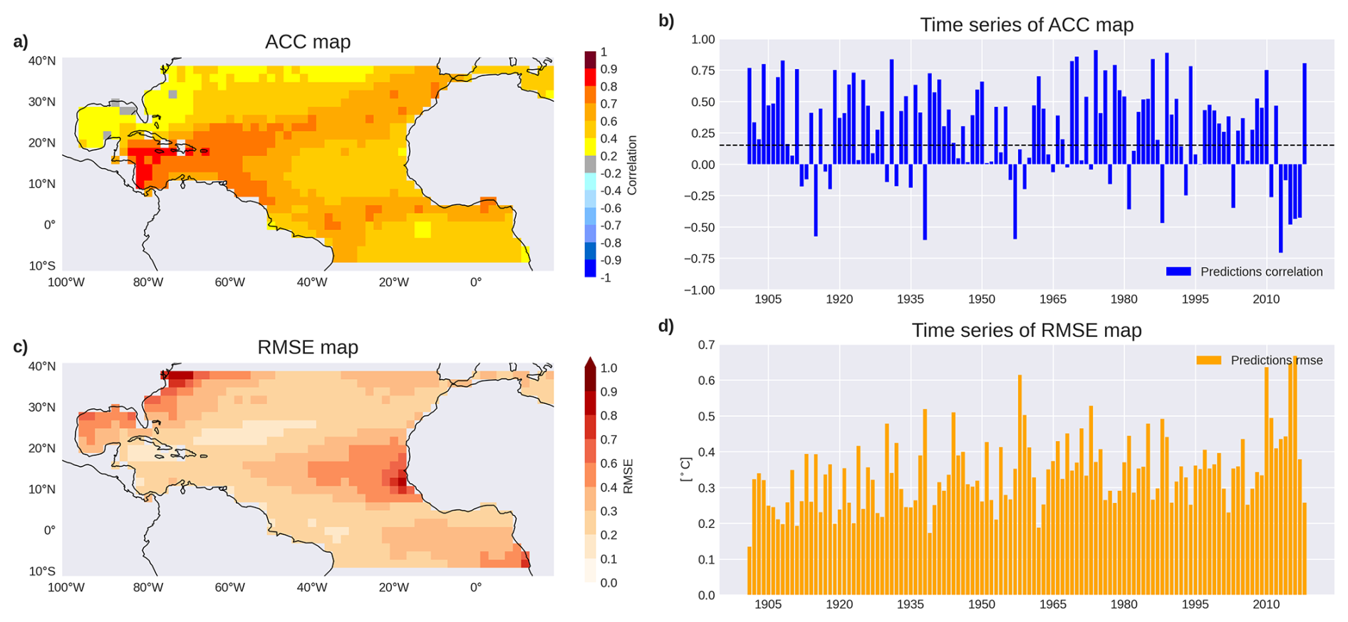
Figure 3 Predictability of tropical North Atlantic SST variability from tropical Pacific anomalies. Panels show model performance over 1901–2019 using leave-one-out cross-validation to predict MAM TNA SST anomalies from DJF tropical Pacific SST anomalies. Predictions are compared with observed MAM SST anomalies. Specifically: (a) spatial anomaly correlation coefficient (ACC) map, computed at each grid point as the temporal correlation (1901–2019) between predicted and observed anomalies; (b) yearly spatial ACC time series, where each value represents the spatial anomaly (pattern) correlation between predicted and observed anomaly fields over the full TNA domain for a given year; (c) spatial RMSE map, computed analogously to (a); and (d) yearly spatial RMSE time series, computed analogously to (b). Shading in (a) indicates statistically significant correlations at the 95 % level (one-tailed t test). The dashed line in (b) marks the corresponding significance threshold.

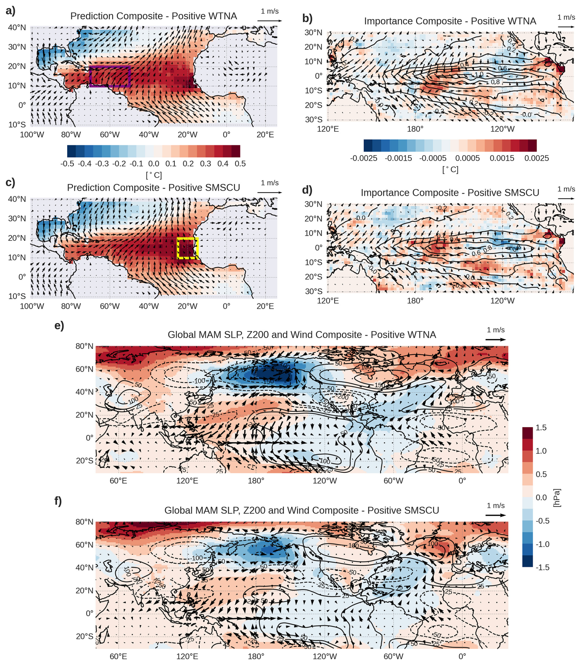
Figure 4 Composites of model anomalous SST predictions, predictor fields, and attribution maps for positive predicted WTNA and SMSCU, based on 28 and 26 events, respectively. Panels (a) and (c) show the predicted mean SST anomalies in the Atlantic during MAM together with surface wind anomalies indicated by arrows. Panels (b) and (d) show the attribution maps over the predictor fields with SST in contours and surface winds in arrows. Panels (e) and (f) display global composites of MAM anomalies in sea level pressure (shading), 200 hPa geopotential (contours), and surface winds for positive WTNA and SMSCU events. Attribution maps indicate the relative contribution of each grid point in the predictor field to the forecasted value in the target region, with the sum of the values within each map matching the predicted anomaly in the corresponding index region – i.e., the sum of all values in panel (c) matches the WTNA anomaly within the purple box in panel (a).

To obtain a robust measure of model performance, we apply a cross-validation approach. This is achieved by enabling the cross-validation argument and specifying the number of folds into which the dataset will be partitioned. Specifically, a leave-one-out cross-validation scheme with 120 folds is employed. The metrics of model performance across the entire hindcast period are summarized in the output figure of the function (Fig. 3). High skill is shown in the whole tropical Atlantic region, with maximum values (up to 0.9) over the western side of the basin (Fig. 3a). Notably, the skill in the TNA region remains positive and ranging from 0.4 to 0.8 in most of the years, with improved performance during certain decades, as during the 1980s, where each yearly value represents the spatial anomaly correlation computed over the full domain (Fig. 3b). In terms of the RMSE (Fig. 3c), three regions stand out where model errors are more pronounced: the Atlantic Niño, the Gulf Stream, and the Mauritanian–Senegalese Coastal Upwelling (SMSCU) system. These areas coincide with regions exhibiting the highest SST variability. Interestingly, the model achieves a high level of skill using only tropical Pacific information, allowing the impact of boreal winter ENSO conditions on the subsequent spring tropical Atlantic state to be quantified. Furthermore, to identify the regions from which the model extracts information to generate the TNA signal, attributions for two regions are computed using the Integrated Gradients method, as outlined in Sect. 2: one representing the western TNA (WTNA) region [10–20° N; 50–70° W], where the model shows higher predictive skill (Fig. 3a), and the other representing the SMSCU system [10–20° N; 25–15° W], where prediction errors are larger (Fig. 3b). These regions were also chosen based on previous research on the impact of ENSO-related teleconnections in both areas (García-Serrano et al., 2017; Wade et al., 2023).

To better understand the model behaviour, we constructed composites based on the WTNA and SMSCU indices, selecting events where the respective indices exceeded ± 0.5 SD (standard deviation). Figure 4 shows composites of different fields for the positive events of both indices. Figure 4a and c displays the predicted Atlantic SST for positive WTNA and SMSCU events, respectively, including surface wind anomalies in MAM to highlight local dynamical changes. The WTNA composite shows weaker wind anomalies close to the African coast, consistent with the weaker predicted SST signal, whereas the SMSCU positive composite reveal a local strengthening of southwesterly winds along the Senegalese coast, which can contribute to a reduction of the coastal upwelling and strong coastal SST warming. Attribution maps highlight that the central Pacific is a major contributor for both WTNA and SMSCU, specifically around 170° E–150° W, with additional positive contributions from the eastern part of the Pacific basin as well as negative contributions from a region located around 130–110° W (Fig. 4b–d). Notice that these spatial patterns should be interpreted as reflecting statistical associations within the learning framework, capturing co-varying large-scale climate signals rather than direct causal influences from individual regions.

The region of positive attributions is coherent with physical mechanisms linking both basins. Indeed, WTNA predicted anomalies corresponds to events in which the central Pacific presents a pronounced wind convergence, consistent with a Gill-type atmospheric response, characteristic of a central Pacific warming (Fig. 4e) (Gill, 1980). This tropical response initiates a broader extratropical wave propagation towards the Atlantic, which is related with a negative NAO-like pattern that weakens the trade winds over the TNA region, particularly for WTNA events (Horel and Wallace, 1981; Czaja et al., 2002). A secondary Gill-type response over the equatorial Atlantic, associated with the anomalous upper-level convergence induced by the modification of the Walker cell, further contributes to the weakening of the trade winds on its western flank and to reduced upwelling. In the case of warm phases of the SMSCU, this secondary Gill response is more regional, and the associated warming could be linked to anomalous negative Ekman pumping, which reduces the upwelling (Calvo-Miguélez et al., 2025). Model predictions and their attributions for two specific samples, 1986 and 1997, as well as composites for the negative phases of WTNA and SMSCU, and Niño3.4-based composites, are provided in the Supplement (Figs. S1–S5).The Supplementary Material also includes regression maps of the WTNA and SMSCU indices onto Pacific SSTs, allowing for comparison with the model attributions.

4.2 Modelling North and Tropical Pacific – European precipitation teleconnection

In this section, we focus on the relationship at the seasonal scale between north and tropical Pacific SST anomalies and European precipitation during boreal autumn (October–November–December; OND), a challenging target variable for dynamical models (Johnson et al., 2019). In the North Atlantic, the dominant mode of atmospheric interannual to decadal variability is the NAO, which modulates the pressure gradient between the Icelandic Low and the Azores High (Rogers, 1997; Trigo et al., 2002). This gradient, in turn, determines the storm tracks over Europe and consequently influences precipitation. Although the NAO signal largely arises from internal variability, external factors such as ENSO can modulate its centers of action via tropospheric and stratospheric pathways (Rodwell et al., 1999; Rodríguez-Fonseca et al., 2016). The interplay with other climate modes, including the Atlantic Multidecadal Oscillation (AMO) and the Pacific Decadal Oscillation (PDO), contributes to the non-stationarity of this teleconnection and, consequently, to the varying influence of ENSO on European precipitation over time (López-Parages and Rodríguez-Fonseca, 2012).

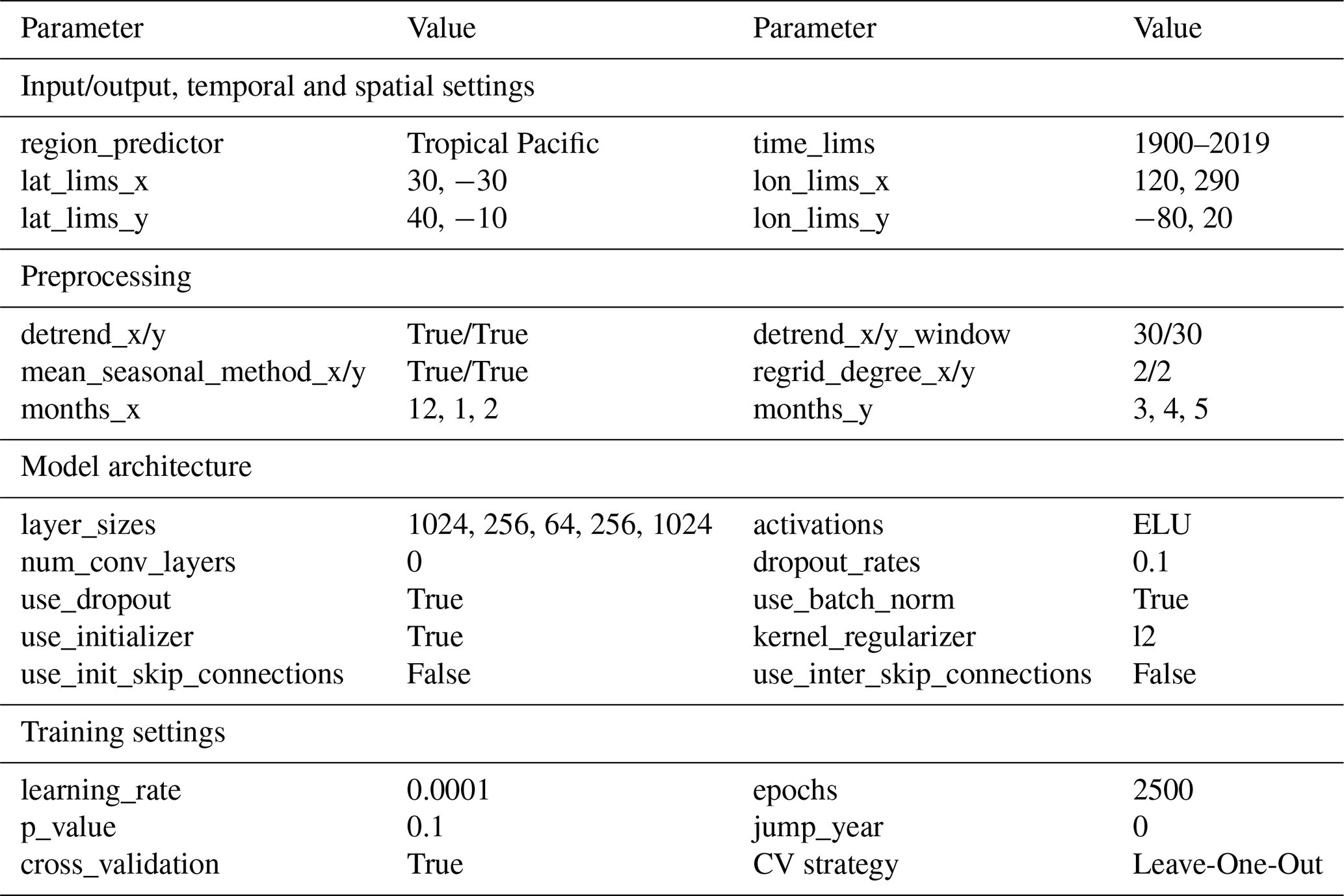
For this analysis, SST data from the HadISST dataset were used as the predictor field (Rayner et al., 2003), while precipitation data from the Climatic Research Unit gridded Time Series (CRU TS) dataset served as the predictand (Harris et al., 2020). Additionally, surface winds (U₁₀, V₁₀) and geopotential and zonal winds at 200 hPa (Z₂₀₀, U₂₀₀) from ERA-20C reanalysis is used for dynamical analysis (Poli et al., 2016). The predictor region covers the Pacific basin [20° S–75° N; 120° E–70° W] to capture the ENSO and extratropical Pacific related variability, while the predictand region is defined by the European continent [35–75° N; 10° W–30° E]. The hyperparameters and other modelling parameters are detailed in Table 3. Unlike the previous case study, precipitation was aggregated from monthly data (by setting the parameter mean₋seasonal₋method₋y = False).

Table 3 Table summarizing the model hyperparameters and preprocessing settings used in the simulation of Pacific SSTs and European precipitation in OND.

After performing a leave-one-out cross-validation, the results are summarized in Fig. 5. The ACC map indicates that only northern Scandinavia, northern Spain and eastern central Europe exhibit significant positive skill (Fig. 5a). The RMSE map indicates higher errors in regions with greater precipitation variability, such as Norway, the United Kingdom and northwestern Spain (Fig. 5c). At first glance, these results might suggest that either the model fails to capture the teleconnection or that the Pacific SST and European precipitation link is inherently non-stationary, as suggested by López-Parages and Rodríguez-Fonseca (2012). The temporal evolution of the ACC and RMSE (Fig. 5b–d), where each yearly value represents the ACC and RMSE computed over the full domain, supports the latter hypothesis; there are periods such as the 1950s–1970s when the model displays considerable skill (ACC > 0.4), contrasted with periods like the 2000s where skill is minimal (ACC ≈ 0).

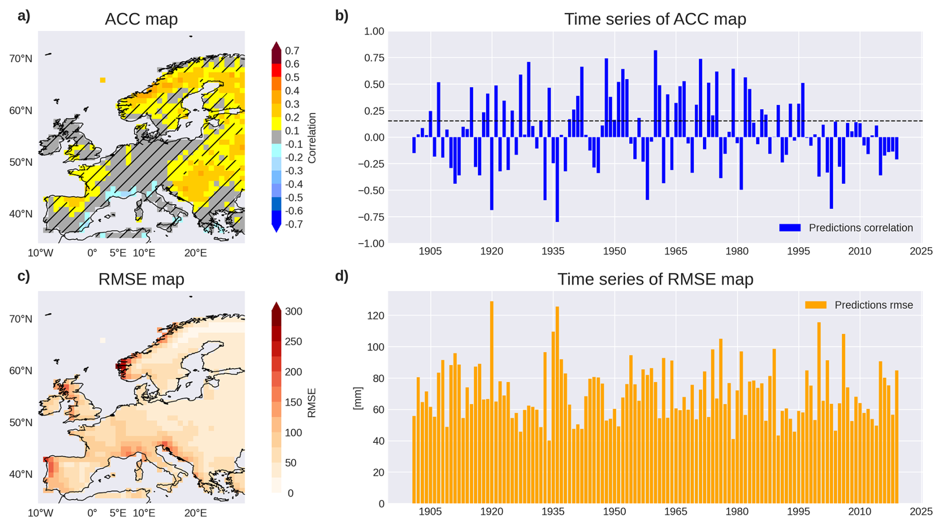
Figure 5 Predictability of European precipitation variability from north and tropical Pacific SST anomalies. Panels show model performance 1901–2019 using leave-one-out cross-validation to predict OND European precipitation anomalies from OND Pacific SST anomalies. Specifically: (a) spatial anomaly correlation coefficient (ACC) map, computed at each grid point as the temporal correlation (1901–2019) between predicted and observed anomalies; (b) yearly spatial ACC time series, where each value represents the spatial anomaly (pattern) correlation between predicted and observed anomaly fields over the full European domain for a given year; (c) spatial RMSE map, computed analogously to (a); and (d) yearly spatial RMSE time series, computed analogously to (b). Shading in (a) indicates statistically significant correlations at the 95 % level (one-tailed t test). The dashed line in (b) marks the corresponding significance threshold.

To gain further insight into the model predictions and to understand the type of European precipitation variability that NN4CAST is capturing, we conduct additional analyses. Concretely, we employ the built-in PC-analysis functionality of NN4CAST to extract the EOFs. The leading mode of variability of the OND precipitation fields, explaining 30 % and 44 % of the total variance in the observational and model prediction datasets respectively, exhibits a coherent spatial pattern, indicating that the model reproduces the variability with remarkable accuracy, although overestimating the relative importance of this leading mode (Fig. 6a and b). In particular, the model effectively captures the core features of this mode, especially in regions where this mode of variability has the higher impacts, such as Scandinavia, the United Kingdom, western Europe, and the Balkans. While a slight underestimation in the overall amplitude is evident, the spatial correlation between the simulated and observed patterns reaches r=0.98, indicating that the model skilfully represents the structure and geographical distribution of the dominant precipitation variability during this season.

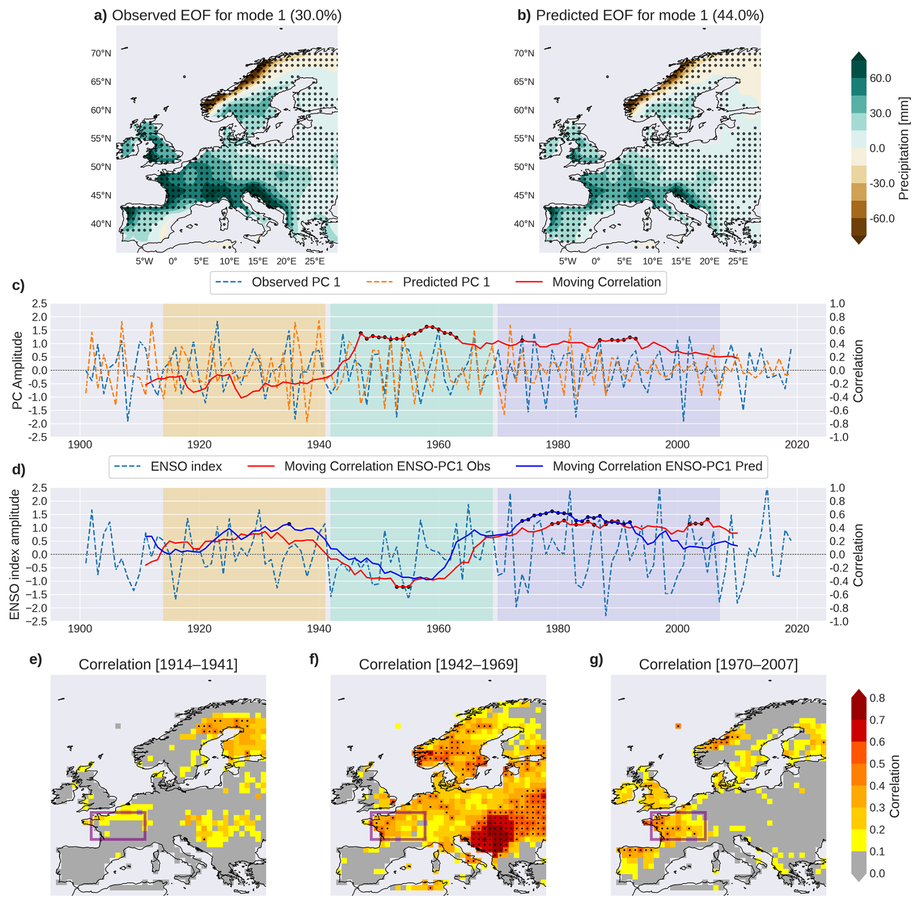
Figure 6 Principal Component Analysis (PCA) of precipitation anomalies over Europe during OND for both observed and predicted datasets. Panels (a) and (b) show the spatial pattern of the first mode of variability for the observed and predicted fields, respectively, with the percentage of explained variance indicated in parentheses. Panel (c) displays the temporal evolution of the principal component (PC) associated with the first mode, representing its high-frequency component after applying a Butterworth filter with a 7-year cut-off, along with the 20-year centered moving window correlation between the observed and predicted PC time series. Panel (d) presents the Niño 3.4 index time series and its 20-year centered moving correlations with both the observed and predicted PCs. Panels (e)–(g) show the ACC maps between the predicted and observed precipitation high-frequency fields (cut-off of 7 years). Dots in each panel indicate points where the regression/correlation is statistically significant at the 95 % confidence level, based on a two-tailed t test. Three shaded periods in panels (c) and (d) indicate intervals selected for further analysis following (López-Parages and Rodríguez-Fonseca, 2012).

To better understand how this variability evolves over time, the associated PC time series were first temporally filtered to retain only their high-frequency components by applying a Butterworth filter with a 7-year cut-off frequency, following the methodology of other works (López-Parages et al., 2015). Twenty-year centered moving-window correlations between the observed and predicted PCs (Fig. 6c) reveal that model skill exhibits limited skill during 1910–1940, improved skill during 1940–1969 (r≈0.4–0.7), and modest skill thereafter 1970–2010 (r≈0.2–0.5). To identify the potential climate driver behind these fluctuations, we then calculated the moving-window correlations between each high-frequency PC and the Niño 3.4 index (Fig. 6d). During the 1940–1969 period of higher skill, the PC-Niño 3.4 correlation is negative, indicating that La Niña events coincide with increased precipitation over western Europe. In contrast, another period of significant correlations shows positive relationships between the leading PC and El Niño. The change in sign across periods indicates how different teleconnections with ENSO can lead to variations in model reliability. Interestingly, a period of reduced skill appears during 1910–1940, with no significant correlation with El Niño in either the observations or the model. These changes in the reliability of the PCs are also reflected in the skill, as evidenced by the ACC maps shown in Fig. 6e–g. These results demonstrate that the model not only reproduces the dominant variability of precipitation, but also captures the non-stationary nature of the ENSO-European precipitation.

Our results coincide with those of López-Parages and Rodríguez-Fonseca (2012), although with minor differences due to changes in data preprocessing. Specifically, while the previous study applied stronger filtering to isolate interannual variability, in the present work we used a Butterworth filter with a cut-off below 7 years, which may retain some lower-frequency variability. Based on the model's ability to reproduce the dominant mode of precipitation variability over Europe (Fig. 6c), we defined three intervals: a low-skill period (1914–1941), a medium-skill period (1970–2007), and a high-kill period (1942–1969). The corresponding composites of model predictions, predictor fields, and attribution maps for positive precipitation events over western-central Europe (purple box in Fig. 7a) are presented in Fig. 7. Composites were constructed by selecting events where the respective anomalous precipitation index exceeded ±0.5 SD.

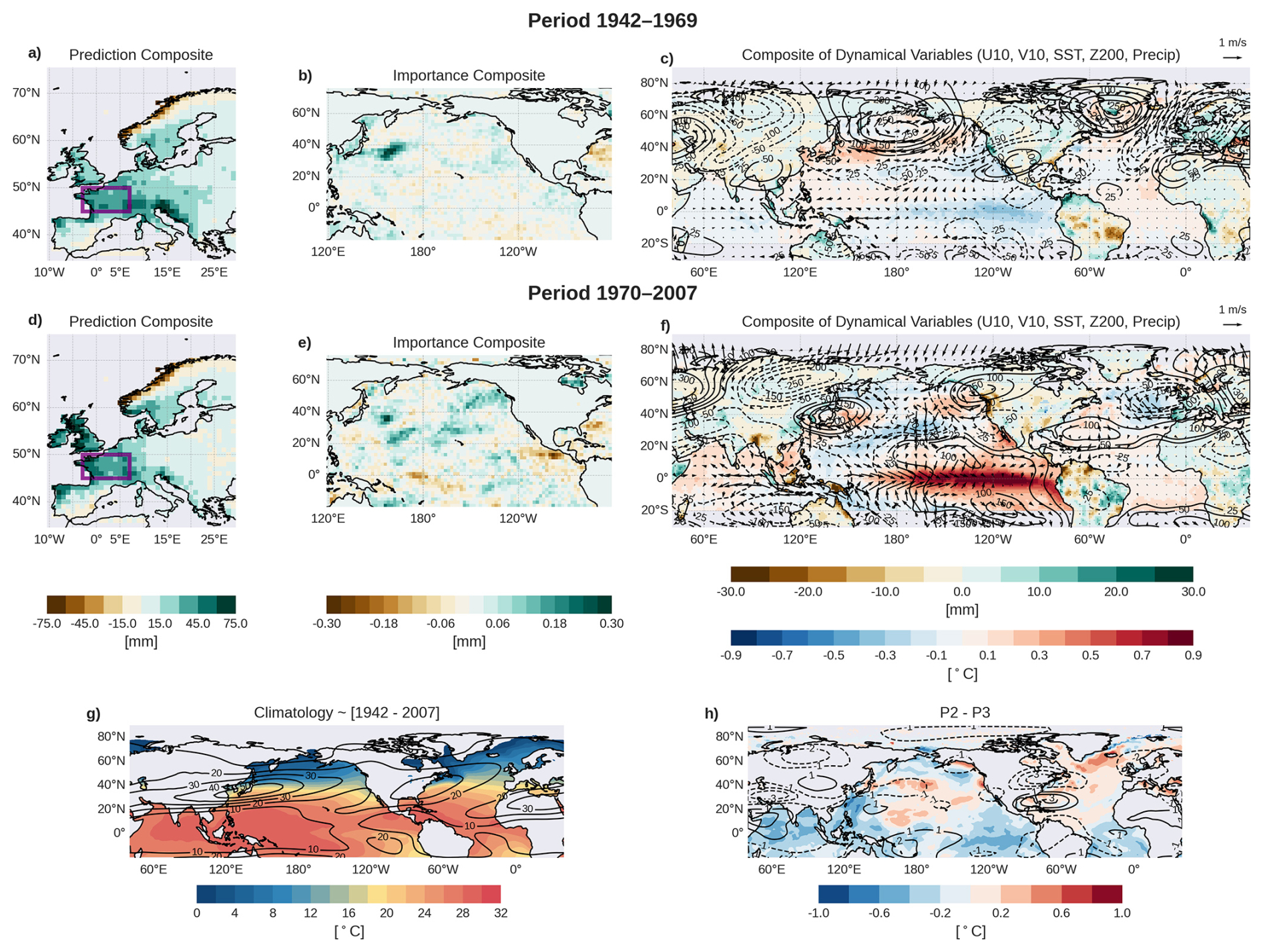
Figure 7 Composites of model predictions, predictor fields, and attribution maps based on positive precipitation events in western central Europe (index defined as the purple rectangle in a), with 11 events in period P2 [1942–1969] and 7 events in period P3 [1970–2007]. Panels show: (a, d) precipitation anomalies in Europe during OND for periods P2 and P3, respectively; (b, e) attribution maps over the predictor field corresponding to positive events for periods P2 and P3, respectively. Panels (c, f) display global composites of OND anomalies in sea surface temperature and precipitation (shading), 200 hPa geopotential (contours), and surface winds for positive events for periods P2 and P3, respectively. Attribution maps (b, e) indicate the relative contribution of each grid point in the predictor field to the forecasted value in the target region. The sum of the attribution values within each map equals the predicted anomaly in the corresponding index region – i.e., the sum of values in panel (b) matches the precipitation anomaly within the purple box in panel (a). Panels (g, h) show the climatology of the SST and U200 for the period [1942–2007] as well as the differences from periods P2 and P3.

The analysis reveals clear differences between the two periods in the teleconnection mechanisms inferred from the modelled precipitation. During P2, rainfall variability is associated with a weak La Niña and enhanced precipitation over regions such as the Maritime Continent. These anomalies could act as sources of Rossby waves, triggering a circumglobal teleconnection pattern. In contrast, during P3, a strong El Niño signal is present, together with a well-defined Gill-type response and an atmospheric Rossby wave train propagating into the extratropics, impacting precipitation over western-central Europe (Fig. 7f). The attribution maps further clarify the regions contributing to the European precipitation signal. During P2, most of the predictive rainfall signal originates from an extratropical region around 40° N and 160° E, consistent with a weakening of the Aleutian Low and with little evidence of direct influence from the equatorial Pacific. The use of lag-0 relationships could explain contributions from multiple ocean basins, reflecting concurrent atmosphere-ocean interactions influencing rainfall variability. In P3, an additional contribution from the tropical Pacific emerges, consistent with the stronger El Niño signal and the enhanced ENSO influence discussed above. Differences in the background climatology, particularly in the meridional SST gradient and the intensity and position of the jet stream (Fig. 7g and h), help explain the distinct teleconnection patterns: P2 is characterized by a weaker meridional gradient and a southward-displaced jet, producing a weaker Pacific-Europe link that is more closely related to a circumglobal response (Branstator, 2002), whereas P3 exhibits a stronger gradient that enables an enhanced teleconnection. These composites highlight how changes in both tropical Pacific forcing and the extratropical background state contribute to variations in model skill and in the mechanisms linking ENSO to European precipitation, all of which are captured by the simulated rainfall. Composites for negative precipitation events reveal a similar but reversed mechanism (see Fig. S6). We note that the diagnosed relationships represent statistical associations learned by the NN model. While the patterns resemble known modes of variability (e.g., ENSO, NAO), they do not imply causal forcing, which would require dedicated sensitivity experiments to isolate individual contributions.

Additionally, composites based on the observed precipitation index show a dynamical behaviour similar to that of the predicted index (not shown). Regarding the role of the NAO, it is important to note that precipitation is predicted from SSTs, and that the ENSO-Europe teleconnection in early winter does not always project onto the NAO. Depending on the period, the ENSO influence can instead manifest as an East Atlantic (EA) pattern (Hou et al., 2023), as observed in P3. There is no clear ENSO forcing on the NAO during P2, when the NAO/EA variability appears to be more internally driven, whereas in P3 it seems to be more strongly forced by SST anomalies. To better identify the drivers of this teleconnection, an analysis of model skill and its attribution as a function of increasing lead time could provide further insight.

5 Conclusions

Seasonal predictions play a crucial role in climate services, offering valuable insights for sectors such as water resource management, energy demand forecasting and agricultural planning, among others. Earth system models make these predictions by taking into account the interactions of the different components of the climate system. Particularly in ocean-atmosphere interactions, the scale of ocean adjustment is slower, which gives predictability to the impacts on the atmosphere. However, seasonal forecasts are subject to different challenges, not only due to the misrepresentation of certain physical processes due to the limited spatio-temporal resolution, but also due to errors in the initial and boundary conditions. An alternative emerges in the statistical approaches trained with observations for performing these simulations. Due to the linear approach of some of the most used statistical models (linear regression, maximum covariance analysis, etc.), deep learning offers an alternative for assessing climate predictability. NN4CAST is specifically designed to overcome some of these limitations. It assesses the sensitivity of a target climate impact variable to variations in drivers operating at seasonal timescales, such as changes in SST anomalies across different regions, and identify the regions from which the model extracts the information.

The present paper demonstrate, by analizing two state of the art teleconnections, the advantages of this modelling framework, not just for producing retrospective hindcasts but also to analyze the sources of skill and identify the regions that gives predictability to the system. NN4CAST primary applications include:

• Providing a versatile and user-friendly tool for ease of implementation and application.

• Modelling relationships between fields, including non-linear components, with performance evaluated using various skill and error metrics.

• Assessing potential predictors and exploring the impact of target variables on specific drivers to enhance predictability.

• Identifying windows of opportunity where relationships between fields exhibit stronger predictability.

• Facilitating the analysis of changes in predictability by examining the model attributions in the predictions.

Two case studies, based on well-known climate teleconnections, have been selected to analyse the potential applications of the proposed tool and pose new hypothesis that could be inferred thanks to this approach. First, the potential predictability of tropical north Atlantic SSTs is assessed training the model with DJF tropical Pacific SSTs, due to the fact of the known that there is a robust teleconnection between ENSO in boreal winter and the following anomalous SSTs in the TNA. Then, the sources of predictability are analysed together with the atmospheric teleconnections that can be inferred from the predicted field. Second, OND seasonal European rainfall simulated by the model training with the contemporaneous SSTs are used to infer hypothesis about the sources of predictability and teleconnection mechanisms, due to the fact that this teleconnection has been found to be non-stationary and changes at decadal timescales. In this context, the model enables the identification of periods of enhanced predictability and provides insights into the potential drivers of such variability. In our first case study, examining the ENSO-TNA SST teleconnection, the model successfully reproduces the canonical relationship with high skill and, through attribution analysis, identifies the central Pacific as a key region of influence that traditional regression methods fail to detect. In the second case study, which assesses the impact of Pacific SSTs on European precipitation, the model accurately captures the non-stationarity behaviour of the teleconnection, achieving the highest skill during the period of negative ENSO – European precipitation correlation and reproducing the dynamical patterns characteristic of that phase.

The case studies presented demonstrate that NN4CAST enables model assessment through performance metrics and visualization tools, which can be used to identify windows of opportunity (WoO) for seasonal prediction. For example, in the European precipitation case study, period P2 (1942–1969) represent a WoO, where predictive skill is high for predicting precipitation. This illustrates how NN4CAST can guide the identification of time intervals in which forecasts are most reliable, supporting more targeted and effective seasonal prediction strategies. Model skill metrics and the analysis of attributions in the predictive field, outcomes of NN4CAST, allow users to better understand climate teleconnections and its underlying physical mechanisms.

The NN4CAST framework further facilitates the implementation of pseudo-sensitivity experiments, whereby users can, for instance, select different SST regions as predictors and evaluate their individual and combined contributions by applying them both jointly and separately. This capability, together with the possibility to vary predictands, and employ different datasets, enhances the framework utility for systematically assessing model sensitivities and robustness. Additionally, this framework is designed to allow the integration of more complex deep learning architectures currently used in meteorological modelling, such as transformers. This capability enables a direct evaluation of the strengths and limitations of each architecture within the modelling framework. Furthermore, plans are underway to extend the NN4CAST framework to additional applications relevant to the scientific community, including integration with tools such as ESMValTool (Righi et al., 2020), thereby enhancing its utility for comprehensive climate model evaluation and diagnostics.