Assessing vertical coordinate system performance in the Regional Modular Ocean Model 6 configuration for Northwest Pacific

The Northwest Pacific (NWP) has a complex ocean circulation system and is among the regions most affected by climate change. To facilitate rapid responses to marine incidents and effectively address climate variability impacts, the Korea Institute of Ocean Science and Technology (KIOST) developed the Korea Operational Oceanographic System–Ocean Predictability Experiment for Marine Environment (KOOS-OPEM), a high-resolution regional ocean prediction system based on Modular Ocean Model version 5 (MOM5). In this study, the base model of KOOS-OPEM was upgraded to MOM6 to enhance its regional ocean modeling capabilities. A key advancement of MOM6 is its flexible vertical coordinate system enabled by a Lagrangian remapping system. Taking advantage of this feature, we evaluated the impact of vertical coordinate choices on model performance by comparing the HYBRID (z^∗-isopycnal) and ZSTAR (z^∗) configurations. Model outputs from the 2003–2012 period were assessed against multiple observational datasets and reanalysis products to determine their ability to reproduce key oceanographic features. The results indicated that HYBRID better preserved stratification and reduced spurious diapycnal mixing, significantly improving the representation of North Pacific Intermediate Water (NPIW). In contrast, ZSTAR exhibited excessive diapycnal mixing, resulting in a thicker isopycnal layer associated with NPIW and a salinity bias of approximately 0.2 psu. An idealized age tracer experiment further confirmed that ZSTAR facilitates excessive downward diffusion of younger surface waters, eroding the minimum salinity layer of the NPIW. In tidal simulations, HYBRID outperformed ZSTAR in reproducing M2 tidal amplitudes in the Yellow Sea, where stratification plays a key role. Conversely, ZSTAR underestimated these amplitudes due to its limitations in representing stratification. Despite its advantages, HYBRID underperformed in high-latitude regions, exhibiting larger temperature and salinity biases between 100 and 600 m depth, with temperature biases reaching approximately −1 °C. This discrepancy arose because HYBRID maintained fewer active layers in weakly stratified regions, reducing vertical resolution and leading to errors in water mass representation. To mitigate these issues and improve HYBRID's performance in high-latitude regions, adjustments to target density profiles are necessary. In addition, both configurations showed limitations in simulating winter SST, largely due to insufficient vertical resolution in the surface mixed layer. To address these issues, adopting a finer surface layer resolution (e.g., 1 m instead of 2 m) will further enhance the model's representation of mixed-layer processes.

1 Introduction

The Northwest Pacific (NWP) Ocean has a complex circulation system characterized by strong western boundary currents, including the Kuroshio and Oyashio Currents, which exhibit significant energetic variability. This region also encompasses several marginal seas, including the South China Sea, the East/Japan Sea, the Yellow Sea, and the East China Sea, which are interconnected through narrow straits (see Fig. 1). Each marginal sea exhibits unique physical oceanographic characteristics shaped by its complex bottom topography and hydrodynamic processes. For instance, the South China Sea, with its deep basins and intricate current system, is strongly influenced by seasonal monsoons and the intrusion of the Kuroshio Current. The East/Japan Sea, a semi-enclosed deep marginal sea with steep underwater topography, shares characteristics with major oceans, including a regional western boundary current (the East Korea Warm Current, EKWC), an intermediate salinity minimum layer, deep water formation via its own ventilation system, and both mesoscale and sub-mesoscale eddies and fronts (Kim and Kim, 1983; Ichiye, 1984; Senjyu, 1999; Kim et al., 2001). The East China Sea, characterized by a broad continental shelf and shallow waters, has circulation patterns driven by wind variations, tides, riverine discharges, and external forcings from the Taiwan and Tsushima Straits, along with Kuroshio Current intrusions (Isobe, 2008; Gan et al., 2016). The Yellow Sea, known for its shallow depths and extensive tidal flats, is dominated by strong tidal currents and seasonal temperature variations, which drive vertical mixing and contribute to the formation and maintenance of the Yellow Sea Bottom Cold Water Mass (YBCWM), a distinct water mass in this marginal sea.

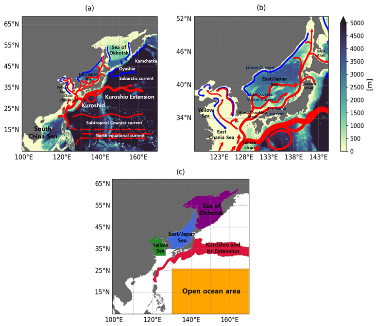
Figure 1 Bottom topography and ocean currents in the Northwest Pacific. (a) Full-region view and (b) zoomed-in view of the marginal seas, including the Yellow Sea, the East China Sea, and the East/Japan Sea, based on data from Park et al. (2010). Red arrows indicate warm currents, while blue arrows represent cold currents. (c) Five distinct regions used for regional temperature and salinity analysis: the open ocean of the Northwest Pacific (orange), the Kuroshio and its Extension (red), and three major marginal seas – Yellow Sea (green), East/Japan Sea (blue), and the Sea of Okhotsk (purple). The Kuroshio and its extension encompasses areas influenced by the Kuroshio Current and its extension, where the climatological surface current speed in GLORYS12 exceeds 0.3 m s⁻¹.

Over the past few decades, rising ocean temperatures have led to a significant increase in sea surface temperature (SST) in the NWP and its marginal seas, exceeding the global average (Belkin, 2009). Additionally, the magnitude and frequency of extreme climate events, such as marine heatwaves and cold surges, have increased markedly in the region (Horton et al., 2015; Oliver et al., 2018; Tan and Cai, 2018; Yamaguchi et al., 2019; Yeo and Ha, 2019; Lee et al., 2020). For example, in July 2021, the NWP experienced a record-breaking marine heatwave, with SST anomalies exceeding 3 °C in parts of the East/Japan Sea and the Sea of Okhotsk compared to the 1982–2011 baseline period (Li et al., 2023). Furthermore, the Kuroshio Current has intensified amid long-term oceanic warming trends (Chen et al., 2019), and its eastward inertial extension, the Kuroshio Extension, has shifted northward, leading to substantial SST increases in surrounding oceans (Kawakami et al., 2023).

To enable rapid responses to extreme marine events and accidents, as well as to address changes in oceanic conditions affecting physical properties and marine ecosystems, the Korea Institute of Ocean Science and Technology (KIOST) developed the high-resolution regional ocean model for the NWP, the Korea Operational Oceanographic System–Ocean Predictability Experiment for the Marine Environment (KOOS-OPEM). The initial version of KOOS-OPEM (Kim et al., 2009; Park et al., 2010) was a regional ocean circulation model for the East/Japan Sea, based on Modular Ocean Model version 3 (MOM3; Pacanowski and Griffies, 1999), with a horizontal resolution of $\mathrm{1}/\mathrm{10}$°. To improve the scientific understanding of the NWP and its marginal seas, KOOS-OPEM underwent multiple enhancements, including an increase in horizontal resolution to $\mathrm{1}/\mathrm{24}$° to resolve the first baroclinic Rossby radius in most regions (Hallberg, 2013), expansion of the model domain, an upgrade from MOM3 to MOM5 (Griffies, 2012), and the incorporation of a data assimilation system based on Ensemble Optimal Interpolation (Kim et al., 2015).

Following these improvements, numerous studies have utilized KOOS-OPEM. Kim et al. (2021) applied an early version of the model to investigate the formation, variability, and pathways of intermediate waters in the East/Japan Sea. Yoon et al. (2022) explored the mechanisms driving summer phytoplankton blooms in Korean coastal waters using model outputs. Chang et al. (2023) assessed the contribution of satellite and in situ temperature observations to high-resolution regional ocean modeling. Additionally, Chang et al. (2024) developed and evaluated a high-resolution regional ocean reanalysis for the NWP, while Jin et al. (2024) examined a 10 d ocean prediction system using KOOS-OPEM, which is operated weekly by KIOST, comparing it with other analysis and forecast fields.

In this study, we updated the base model of KOOS-OPEM to MOM6 (Adcroft et al., 2019), the latest version of MOM, to enhance its capabilities. MOM6 introduces a significantly different algorithm compared to previous versions (up to MOM5) and offers substantial improvements in computational efficiency and stability. A key advancement is its use of vertical Lagrangian remapping (Griffies et al., 2020), a variant of the Arbitrary Lagrangian–Eulerian (ALE) algorithm, which allows for the implementation of various vertical coordinate systems, including geopotential (z or z^∗), isopycnal, terrain-following, or hybrid/user-defined coordinates. MOM6 also adopts a C-grid discretization instead of the previous B-grid and updates the ocean boundary layer parameterization from the traditional K-Profile Parameterization (Large et al. 1994) to the energetically consistent planetary boundary layer (ePBL) scheme (Reichl and Hallberg, 2018), further improving vertical mixing representation and surface–interior coupling. Additionally, newly developed open boundary conditions and improved regional modeling capabilities in MOM6 facilitate its effective use in regional ocean models.

Several recent studies have successfully implemented MOM6 in regional ocean modeling applications. Ross et al. (2023) conducted a hindcast simulation using MOM6 with the Sea Ice Simulator version 2 (SIS2) and the Carbon, Ocean Biogeochemistry, and Lower Trophics (COBALT; Stock et al., 2020) biogeochemistry model for the Northwest Atlantic from 1993 to 2019. Their simulation demonstrated excellent performance in reproducing physical properties, such as SST and Gulf Stream dynamics, while also exhibiting notable skill in modeling tidal behaviors and complex biogeochemical processes. Seijo-Ellis et al. (2024) applied MOM6 in a high-resolution ($\mathrm{1}/\mathrm{12}$°) regional ocean modeling study of the Caribbean (CARIB12), effectively capturing the region's mesoscale variability, including eddy activity and the dynamics of major currents such as the Caribbean Current and the Loop Current. Furthermore, Drenkard et al. (2025) implemented MOM6-COBALT for the Northeastern Pacific (Seelanki et al., 2025), covering the region from the Chukchi Sea to the Baja California Peninsula at a 10 km horizontal resolution. Their simulations successfully replicated key ecosystem-relevant properties, including temperature, salinity, nutrient distributions, and chlorophyll concentrations, highlighting the model's capability to provide regionally tailored projections and support marine resource management. Additionally, Liao et al. (2025) introduced MOM6-COBALT-IND12, a coupled physical-biogeochemical model for the northern Indian Ocean, which successfully represented monsoon-driven variability, coastal upwelling, and key ecosystem dynamics.

Spurious mixing in ocean models is a major concern, as it introduces an unphysical process that unintentionally increases total mixing beyond the prescribed and parameterized levels (Griffies et al., 2000; Ilıcak et al., 2012; Gibson et al., 2017). Consequently, minimizing spurious mixing is a key focus in model development and configuration, with the choice of the vertical coordinate system playing a crucial role in determining its magnitude. The z^∗ coordinate system (Adcroft and Campin, 2004, hereafter referred to as ZSTAR), as used in MOM5 and Ross et al. (2023), closely resembles the geopotential coordinate by scaling the vertical coordinate proportionally to sea surface height (SSH), allowing the upper ocean layers to remain thin. This characteristic makes it particularly effective for capturing detailed processes in the ocean's mixed layer. Hybrid coordinates combine the advantages of different vertical coordinate systems to optimize model performance. A hybrid z^∗-isopycnal coordinate system (hereafter referred to as HYBRID), motivated by Bleck (2002), employs isopycnal coordinates in the ocean interior, where stratification is prominent, and ZSTAR coordinates in the unstratified mixed-layer regions. The HYBRID approach leverages the benefits of z-level coordinates for high resolution in the upper ocean while using isopycnal coordinates in the deep ocean to minimize diapycnal mixing.

The influence of vertical coordinate systems on ocean circulation has been investigated through a series of idealized and global modeling studies. Chassignet et al. (1996) first compared z-level and isopycnal models for the Atlantic, showing that isopycnal coordinates better preserved water-mass structures and thermohaline circulation. Park and Bryan (2000, 2001) extended these analyses using idealized thermally driven basin experiments, demonstrating that isopycnal-layer models maintained surface stratification and subpolar gyres more realistically than z-coordinate systems. Idealized process experiments, such as those by Legg et al. (2006) and Gibson et al. (2017), further revealed that z-level and z^∗ models are prone to excessive numerical diapycnal mixing and entrainment compared to isopycnal-based schemes, particularly in overflow and strongly stratified regimes. At the global scale, Adcroft et al. (2019) showed that the HYBRID z^∗-isopycnal coordinate in MOM6 effectively reduced mid-depth warming drift and spurious mixing relative to the pure ZSTAR configuration. Despite these advances, systematic evaluations of vertical coordinate systems in regional ocean models remain limited, especially in domains with complex bathymetry, strong tidal forcing, and seasonally varying stratification – conditions that can strongly modulate the balance between vertical mixing and circulation.

In this study, we conducted sensitivity experiments to compare the performance of the HYBRID and ZSTAR coordinate systems in a regional ocean model using the next-generation KOOS-OPEM (OPEM-MOM6). Although MOM6 can employ terrain-following coordinate systems, which are commonly used in regional ocean models, we excluded this option due to its poor performance associated with pressure gradient errors in regions with steep topography, such as the East/Japan Sea (Haney, 1991; Beckmann and Haidvogel, 1993; Mellor et al., 1994; Chu and Fan, 1997; Mellor et al., 1998; Ezer et al., 2002). Therefore, our focus was on assessing the HYBRID and ZSTAR coordinate systems. Our primary objective was to evaluate how these systems influence the model's ability to capture key oceanographic features, processes, and dynamics through a quantitative analysis of their effects.

Section 2 describes the model configuration, including the implementation of different vertical coordinate systems, along with the observational and reanalysis datasets used for evaluation. Section 3 presents the results of the sensitivity experiments, comparing the performance of the HYBRID and ZSTAR configurations in reproducing key oceanographic features. Section 4 discusses the findings and provides interpretations of the mechanisms driving the differences between the two configurations. Finally, Sect. 5 summarizes the main conclusions and suggests potential improvements

2 Methods

2.1 Model configuration

OPEM-MOM6 incorporates coupled model components using MOM6 for ocean physics and SIS2 for sea ice dynamics. The Arakawa-C grid system (Arakawa and Lamb, 1977) with 1704 × 1392 tracer points was used to solve the primitive equations under the Boussinesq and hydrostatic approximations. The model domain encompassed the NWP region, spanning from 5 to 63° N to 99 to 170° E. The model had a horizontal resolution of $\mathrm{1}/\mathrm{24}$° in both longitude and latitude, equivalent to approximately 4 km. The bathymetry data were constructed by integrating the General Bathymetric Chart of the Oceans (GEBCO) 2024 and the KorBathy30s dataset, a regional bathymetry dataset for the Korean Peninsula (Seo, 2008). The minimum bathymetric depth was set to 10 m to account for tidal variations, as wetting and drying were not employed, while the maximum depth was limited to 5000 m to enhance efficiency of vertical grid utilization.

To integrate the ocean model forward in time, a split explicit method (Hallberg, 1997; Hallberg and Adcroft, 2009) was employed, efficiently separating the handling of fast and slow processes. The baroclinic time step was set to 300 s, while the barotropic time step varied and was determined as the largest integer fraction of the baroclinic time step required for stability. A longer time step of 900 s was applied for thermodynamic calculations.

In this study, two vertical coordinate systems, HYBRID and ZSTAR, were configured with 75 layers. Both configurations featured the finest vertical resolution near the surface. In ZSTAR, the layer thickness gradually increased with depth, reaching a maximum of 349.43 m just above the deepest model depth of 5000 m, and the bottom topography was represented using partial-step layers to better capture sloping bathymetry and improve pressure-gradient consistency.

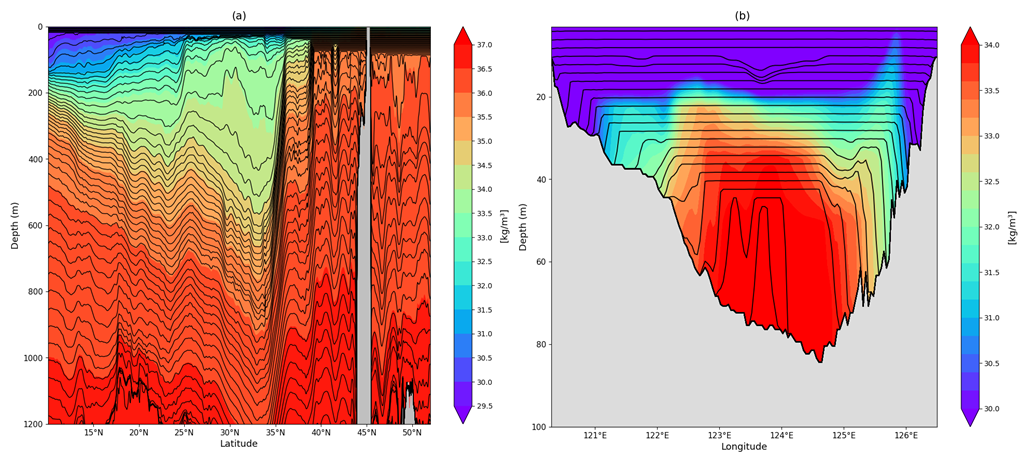
Figure 2 Schematic representation of the simulated HYBRID model interfaces and potential density (referenced to 2000 dbar). (a) Meridional section along 148° E showing vertical grid interfaces overlaid on potential density (kg m⁻³). (b) Zonal section along 36° N across the Yellow Sea, illustrating the vertical grid structure adapted to shallow topography.

In the HYBRID configuration, ZSTAR was used to effectively resolve the mixed layer in unstratified regions, providing high resolution where vertical mixing and surface interactions were most significant. Below the mixed layer, isopycnal coordinates were employed to minimize spurious diapycnal mixing and accurately represent the stratified conditions found in deeper waters. The HYBRID in MOM6 is implemented through a column-wise algorithm that combines the strengths of both approaches. In each water column, a stable, monotonic density profile is first derived from temperature, salinity, and pressure and mapped onto a prescribed set of target densities to obtain isopycnal candidate interface depths. Independently, a nominal ZSTAR grid is defined and used as a one-sided lower-bound constraint for each layer. At every vertical level, the model selects the deeper of the two, either the isopycnal candidate or the ZSTAR floor, and then applies bottom and optional thickness/depth limits. As a result, there is no discrete switch between coordinate systems: the transition depth naturally occurs where an isopycnal surface would otherwise lie above the ZSTAR floor. Because mixed layers are deeper and stratification weaker at higher latitudes, the crossing with the ZSTAR floor occurs at greater depths, leading to a poleward deepening of the transition layer. Over continental shelves, the strength of the ZSTAR constraint scales with the local depth. In shallow regions this scaling makes the ZSTAR floor very shallow, so when residual stratification exists, the interfaces tend to follow the target isopycnals through most of the water column. The overall structure of the model interfaces and their interaction with topography are illustrated in Fig. 2, which schematically shows how the HYBRID coordinate transitions from ZSTAR near the surface to isopycnal layers in the ocean interior.

In MOM6, HYBRID assigned a target density referenced to 2000 dbar for each interface. The choice of a 2000 dbar reference pressure is widely accepted, as it balances monotonicity in near-surface waters with stability in the deep ocean (Megann, 2018) and maximizes the neutrality of isopycnal surfaces (McDougall and Jackett, 2005). However, variations in the vertical density distribution across global and regional scales led to inefficient resolution use, particularly in weakly stratified regions. To address this, 1 % of the compressibility was artificially retained but centered at 2000 dbar when generating the vertical grid at each time step (Adcroft et al., 2019). In this study, the target density ranged from 1010 to 1037.2479 kg m⁻³ referenced 2000 dbar, specifically constructed for the Northwest Pacific rather than using the global target density adopted in OM4.0 (Adcroft et al., 2019).

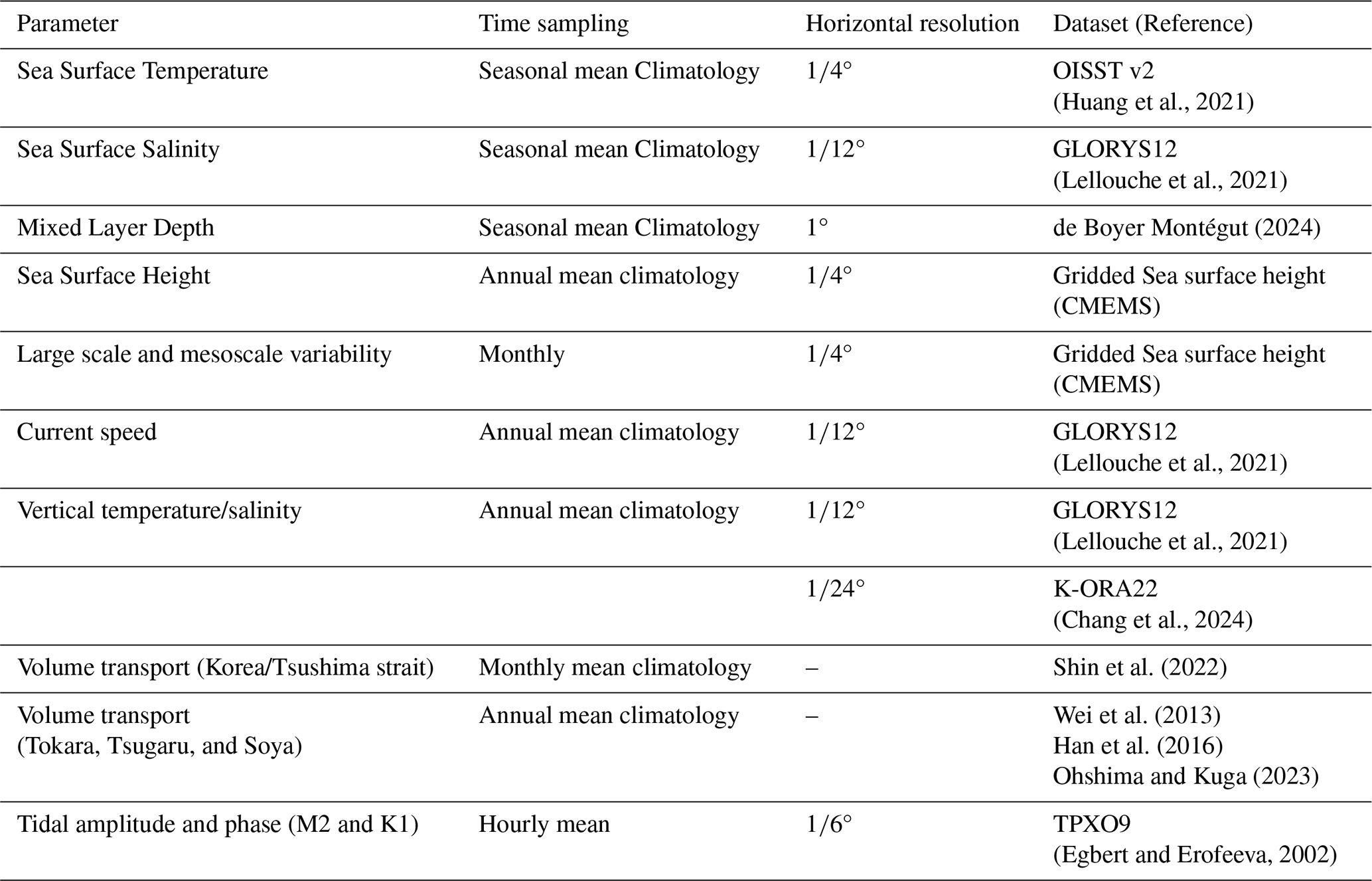
Table 1 Summary of model configuration and parameters for each experiment.

The physical subgrid-scale parameterization settings followed those of Adcroft et al. (2019) and Ross et al. (2023). The ePBL scheme developed by Reichl and Hallberg (2018), with updates accounting for Langmuir turbulence (Reichl and Li, 2019), was employed to parameterize the planetary boundary layer. To parameterize mixed-layer restratification by sub-mesoscale eddies, the scheme proposed by Fox-Kemper et al. (2011) was used, with a frontal-length scale of 1500 m applied for the upscaling of buoyancy gradients. A biharmonic form of horizontal viscosity was used in these simulations. The viscosity was calculated as the maximum value between a biharmonic Smagorinsky viscosity (Griffies and Hallberg, 2000) and a predefined fixed viscosity expressed as u₄Δx³, where u₄ represents a velocity scale and Δx denotes the local grid spacing. The velocity scale was set to 0.01 m s⁻¹, with a Smagorinsky coefficient of 0.015. Shear-driven turbulence mixing was parameterized by Jackson et al. (2008). The bottom friction was represented using a quadratic drag formulation with a coefficient C_D = 0.003. Lateral solid boundaries employed free-slip conditions, allowing tangential flow along the wall while preventing normal flow. Table 1 provides a summary of the model configurations and parameters.

2.2 Model forcing and spin-up

Both configurations were forced using lateral open boundary conditions from the GLORYS12 reanalysis (Lellouche et al., 2021). The variables used for lateral boundary conditions included daily mean temperature, salinity, sea surface height (SSH), and ocean velocity. The model was forced by astronomical tidal potential forcing, with explicit tidal forcing from boundary conditions rather than parameterized tidal mixing. Tidal harmonics, including four semidiurnal (M2, S2, N2, and K2), four diurnal (K1, O1, P1, and Q1), and two long-period (Mm and Mf) constituents from the TPXO9 v1 dataset (Egbert and Erofeeva, 2002), were applied to impose tidal variations in sea level and velocity on the subtidal boundary data. These 10 constituents were also applied as body forces in the momentum equations to simulate astronomical tidal forcing across the domain. Combined tidal and subtidal sea levels, along with barotropic velocities, were prescribed using the radiation boundary conditions described by Flather (1976). For baroclinic flow, a radiation scheme based on Orlanski (1976) was applied, incorporating nudging toward external data following the approach outlined by Marchesiello et al. (2001).

Inflow boundary velocities were strongly constrained with a 3 d nudging timescale, while outflow velocities were weakly adjusted using a 360 d timescale. Temperature and salinity at the boundaries were managed using a reservoir scheme, which adapted boundary conditions based on the internal model state for outflow and external forcing for inflow. The reservoir length scale was set to 9 km.

Surface fluxes between the ocean and atmosphere were derived from hourly ERA5 reanalysis data (Hersbach et al., 2020), including variables such as 2 m air temperature, specific humidity, surface net solar and thermal radiation, mean sea level pressure, total cloud cover, 10 m wind velocity, and precipitation, using the bulk formula from Large and Yeager (2004). River discharge was prescribed using the GloFAS reanalysis version 3.1 (Alfieri et al., 2020). Following the approach of Ross et al. (2023), river discharge was mapped onto the MOM6 grid by identifying coastal outlet points and assigning streamflow to the nearest ocean grid cell using a local drain direction map. A comparison with observations from Datong station revealed that the GloFAS dataset overestimated the Yangtze River discharge. To correct this bias, GloFAS discharge data were adjusted using a bias correction based on the monthly climatological runoff ratio. Freshwater, with zero salinity and a temperature equal to the surface temperature of the discharge grid cell, was added at the surface. Additionally, turbulent kinetic energy was introduced to mix the water column up to a depth of 5 m at discharge points.

Both configurations were initialized using temperature and salinity fields from GLORYS12, which were interpolated to the model grid from 1 January 1993. The spin-up simulation was run for 10 years (1993–2002) using time-varying open boundary and surface atmospheric forcing data. Following the spin-up period, hindcast simulations were performed for 2003–2012 to capture and analyze oceanographic conditions and dynamics. This approach ensured that the models were sufficiently spun up and provided a reliable representation of ocean conditions during the specified period.

2.3 Evaluation

The performance of each configuration was evaluated using observational data and physical reanalysis datasets that assimilated observations. For statistical evaluation, Iris v3.1.0 (Hattersley et al., 2023), a Python package for analyzing and visualizing multi-dimensional meteorological and oceanographic datasets, was used to compare both configurations with the reference dataset. For visualization, Cartopy (Met Office, 2022) was employed to represent geographic features, while Iris was utilized to display the computed variable distributions.

Since reference datasets generally had a lower spatial resolution than the model outputs, model outputs from both configurations were conservatively re-gridded onto the coarser-resolution reference dataset grid using Iris before conducting statistical analysis. The statistical evaluation included spatial mean bias (Bias), root mean squared error (RMSE), median absolute error (MedAE), and the Pearson correlation coefficient (Corr). Bias indicated whether the model systematically overestimated or underestimated values. RMSE quantified the overall discrepancy between the model and reference datasets by measuring squared differences, making it sensitive to large errors. In contrast, MedAE provided a robust measure of error by calculating the median of absolute differences, reducing the influence of outliers compared to RMSE. Corr measured similarity in spatial or temporal patterns, ranging from −1 (inverse correlation) to 1 (perfect correlation), independent of magnitude differences.

To compare SST from both configurations, the NOAA $\mathrm{1}/\mathrm{4}$° daily Optimum Interpolation Sea Surface Temperature (OISST) dataset, which interpolates and extrapolates observations from satellites, Argo floats, ships, and buoys, was used to evaluate SST performance in the experiments. Sea surface salinity (SSS) validation was conducted using the GLORYS12 reanalysis dataset. Although observational data for SSS are limited, alternative datasets, such as the CMEMS Multi-Observation Global Ocean Sea Surface Salinity product, have been used in previous studies (e.g., Seijo-Ellis et al., 2024). However, the CMEMS product relies on climatological data for coastal areas, where observational coverage is sparse and uncertainty is high. Specifically, the coastal dataset incorporates pseudo-observations derived from climatological backgrounds within 200 km of the coast, as described in CMEMS documentation. In contrast, GLORYS12 has been shown to exhibit relatively low bias around the Korean Peninsula when compared with in-situ observations (Chang et al., 2023), and also demonstrated reasonable temporal variability when compared with SSS time series from the IEODO Ocean Research Station, located in East China Sea (not shown here). Based on these findings, GLORYS12 was deemed a suitable reference for SSS validation in this study.

The marginal seas of the NWP are heavily influenced by significant freshwater discharge from the Yangtze and Yellow Rivers, which creates extensive low-salinity areas that play a critical role in regional salinity distribution and stratification. Therefore, validating SSS in coastal regions is essential for accurately assessing model performance. Given its consistency in representing salinity distributions across both coastal and open-ocean areas, the GLORYS12 reanalysis dataset was selected as the reference.

Table 2 Summary of parameters and dataset used in the evaluation.

The boreal winter and summer mixed layer depth (MLD) was compared to the long-term MLD climatology constructed from World Ocean Database and Argo profiles (de Boyer Montégut, 2024). In this dataset, MLD is calculated using the Δ 0.03 kg m⁻³ density criterion relative to surface density. The MOM6 diagnostic MLD_003 was used for validation, defining MLD as the depth where potential density exceeds the density at 10 m by 0.03 kg m⁻³.

To evaluate sea surface height (SSH) variability, monthly absolute dynamic topography (ADT) data from CMEMS were used. These data, produced by merging SSH observations from various satellite altimetry sources, have a horizontal resolution of 0.25°. Additionally, GLORYS12 was used to validate surface current speed and eddy kinetic energy (EKE) in the model simulations. The EKE for each experiment was calculated by interpolating velocity data onto the AVISO geostrophic current data grid and applying the following equation:

$$\text{EKE}={\displaystyle \frac{\mathrm{1}}{\mathrm{2}}}\left(u^{\prime \mathrm{2}}+v^{\prime \mathrm{2}}\right)$$

where u^′2 and v^′2 represent deviations of the zonal and meridional velocity components from their respective means over the evaluation period (2003–2012).

To assess the model's ability to reproduce tides, the tidal amplitudes and phases of the M2 (semidiurnal) and K1 (diurnal) constituents were calculated using hourly SSH output with the UTide Python package (Codiga, 2011). The results were then compared with TPXO9, which served as the tidal boundary condition.

Additionally, two reanalysis datasets, GLORYS12 and KOOS-OPEM ReAnalysis 2022 (K-ORA22; Chang et al., 2024), were used to evaluate the performance of each experiment in reproducing vertical temperature and salinity structures. A comparative evaluation by Chang et al. (2023) assessed multiple NWP reanalysis datasets, finding that GLORYS12 exhibited the best performance in reproducing temperature, salinity, and large-scale/mesoscale variability. Meanwhile, K-ORA22 demonstrated superior performance in representing marginal seas, particularly excelling in the Yellow Sea. Given these complementary strengths, GLORYS12 and K-ORA22 were selected as reference datasets for evaluating vertical temperature and salinity structures.

To compare regional variations in temperature and salinity between the two configurations, the analysis was divided into five distinct regions, as shown in Fig. 1c:

1. Open ocean area of the NWP,

2. Kuroshio and its Extension,

3. Sea of Okhotsk,

4. East/Japan Sea, and

5. Yellow Sea

The Kuroshio and its Extension regions were defined not only based on areas where the climatological surface current speed in GLORYS12 exceeds 0.3 m s⁻¹ but also by including adjacent regions dynamically affected by the K-KE. A summary of the parameters and datasets used in the evaluation is provided in Table 2.

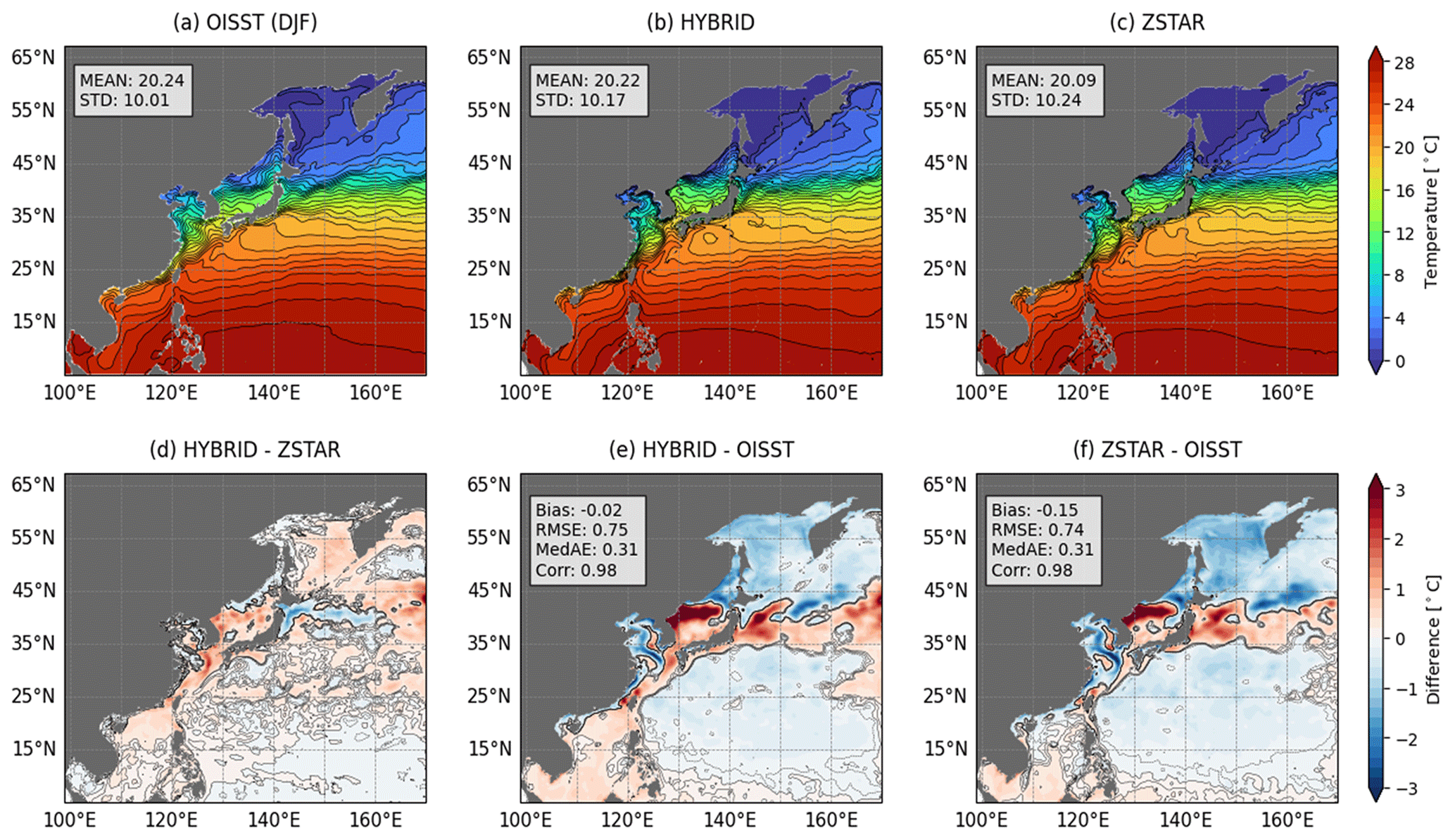
Figure 3 Boreal winter (DJF) mean sea surface temperature (SST) distributions from OISST observations and HYBRID and ZSTAR simulations. (a–c) Spatial SST distributions with corresponding means and standard deviations (STD). (d) Differences between HYBRID and ZSTAR. (e, f) Biases relative to OISST, including Bias, RMSE, MedAE, and Corr. Contour lines in (d)–(f) indicate SST biases ranging from −0.1 to 0.1 °C at 0.1 °C intervals.

3 Results

3.1 Near-surface physical ocean properties

Figure 3 compares the SST distributions for boreal winter (DJF) between the OISST observational dataset and simulations from the HYBRID and ZSTAR configurations. The winter mean SST distributions from OISST and both model configurations exhibited strong agreement in both spatial structure and magnitude across the NWP. Biases relative to OISST were low, with HYBRID showing a bias of −0.02 °C and ZSTAR showing a bias of 0.15 °C, indicating overall consistency with observations. Despite this broad agreement, regional biases were evident. In higher latitudes north of 45° N, both configurations exhibited a moderate cold bias of approximately −0.8 °C, with ZSTAR displaying a more pronounced cold bias compared to HYBRID. Warm biases were observed in the Kuroshio and the Kuroshio–Oyashio transition zone, reaching up to 2.0 °C in both configurations. However, this warm bias was more prominent in the HYBRID configuration, particularly in the Kuroshio–Oyashio transition zone. Additionally, the HYBRID configuration exhibited a warm bias in the South China Sea, whereas the ZSTAR configuration demonstrated a more substantial warm bias exceeding 3.0 °C in the East/Japan Sea, which was notably larger than in HYBRID. Statistical metrics further supported the agreement between the models and OISST. Both configurations achieved high spatial correlations of 0.98, with RMSE values of 0.75 °C for HYBRID and 0.74 °C for ZSTAR. MedAE were 0.31 °C for HYBRID and 0.31 °C for ZSTAR, reflecting similar levels of accuracy in representing SST variability across the region.

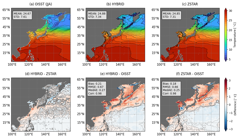
Figure 4 Boreal summer (JJA) mean sea surface temperature (SST) distributions from OISST observations and HYBRID and ZSTAR simulations. (a–c) Spatial SST distributions with corresponding means and STD. (d) Differences between HYBRID and ZSTAR. (e, f) Biases relative to OISST, including Bias, RMSE, MedAE, and Corr. Contour lines in (d)–(f) indicate SST biases ranging from −0.1 to 0.1 °C at 0.1 °C intervals.

Figure 4 presents a comparison of SST distributions for boreal summer (JJA) between OISST observations and simulations from the HYBRID and ZSTAR configurations. Both configurations exhibited similar performance, with RMSE values of 0.67 °C for HYBRID and 0.66 °C for ZSTAR, and both maintained high correlations with OISST (Corr = 0.98), consistent with their performance in winter. However, unlike in winter, both models exhibited warm biases, particularly in the Yellow Sea and high-latitude regions, where biases of approximately 1.0 °C were observed. In contrast, biases in the open ocean of the NWP remained relatively low, typically below −0.3 °C.

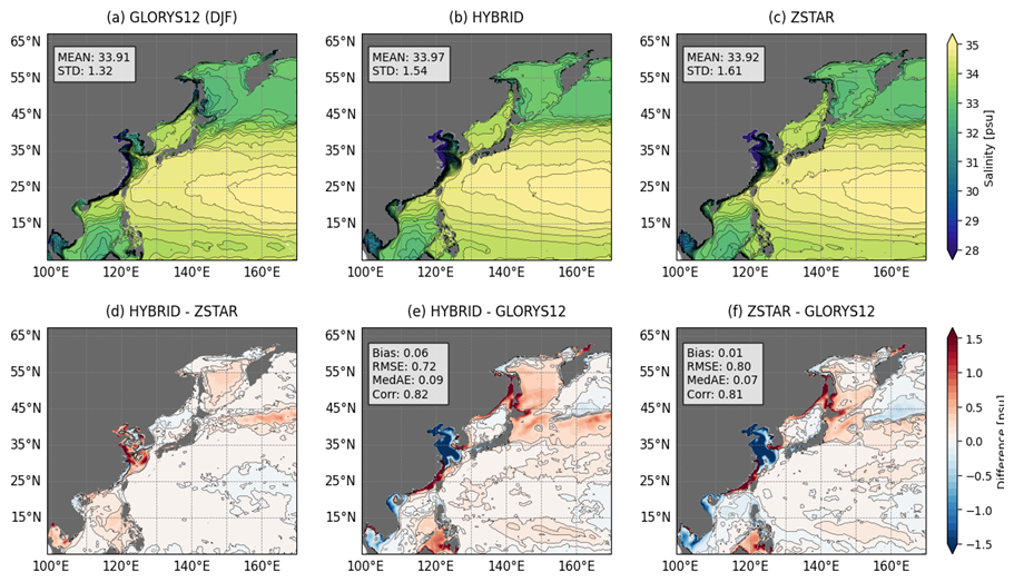
Figure 5 Boreal winter (DJF) mean sea surface salinity (SSS) distributions from the GLORYS12 reanalysis and HYBRID and ZSTAR simulations. (a–c) Spatial SSS distributions with corresponding means and STD. (d) Differences between HYBRID and ZSTAR. (e, f) Biases relative to GLORYS12, including Bias, RMSE, MedAE, and Corr. Contour lines in (d)–(f) indicate SSS biases ranging from −0.1 to 0.1 psu at 0.1 psu intervals.

The simulated mean SSS values for both HYBRID and ZSTAR configurations (33.97 psu) aligned closely with the GLORYS12 reference mean (33.92 psu), demonstrating good agreement in the large-scale salinity distribution across the NWP (Fig. 5). However, the standard deviations (STD) revealed slightly higher variability in the models, with values of 1.54 psu for HYBRID and 1.61 psu for ZSTAR, compared to 1.32 psu in GLORYS12. This indicated that while both models captured regional salinity gradients reasonably well, they tended to overestimate variability.

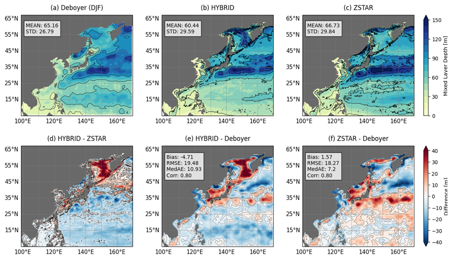
Figure 6 Boreal winter (DJF) mean mixed layer depth (MLD) distributions from de Boyer Montégut and HYBRID and ZSTAR simulations. (a–c) Spatial MLD distributions with corresponding means and STD. (d) Differences between HYBRID and ZSTAR. (e, f) Biases relative to de Boyer Montégut, including Bias, RMSE, MedAE, and Corr. Contour lines in (d)–(f) indicate MLD biases ranging from −0.1 to 0.1 m at 0.1 m intervals.

Regional biases were evident in specific areas. In the Yellow Sea, both configurations exhibited a pronounced negative bias exceeding −1.0 psu, suggesting that excessive freshwater discharge from nearby rivers led to an overestimation of low-salinity water in this region. Conversely, positive biases dominated in the South China Sea, the southeastern Chinese coast, the northern East/Japan Sea, and Sea of Okhotsk, with values exceeding 1.0 psu in some locations. ZSTAR exhibited larger biases than HYBRID in the Yellow Sea, and HYBRID exhibited larger biases than ZSTAR in the South China Sea, the Sea of Okhotsk, and the Kuroshio–Oyashio transition zone. A quantitative comparison with GLORYS12 highlighted differences in model performance. HYBRID achieved a lower RMSE of 0.72 psu compared to 0.80 psu for ZSTAR, suggesting better overall agreement with the reference dataset. Additionally, HYBRID showed a marginally higher spatial correlation with GLORYS12 (0.82) compared to ZSTAR (0.81).

During summer (JJA), the SSS distribution remained similar to winter, with both configurations aligning well with GLORYS12 but showing slightly higher variability (Fig. S1 in the Supplement). The negative bias in the Yellow Sea intensified, exceeding −1.0 psu, while regional bias patterns persisted, with HYBRID showing stronger positive biases in the open ocean and HYBRID exhibiting more negative biases in the Kuroshio–Oyashio transition zone and Sea of Okhotsk. The pronounced fresh bias in the Yellow Sea that, despite applying bias corrections for Yangtze River discharge, river discharge forcing in both configurations may have still been overestimated for other rivers, such as the Yellow River. Therefore, further investigation into discharge from other major rivers is necessary, comparing them with observational datasets for potential corrections.

Figure 6 compares the MLD distributions for boreal winter (DJF) between the estimates of de Boyer Montégut et al. (2024) and simulations from the HYBRID and ZSTAR configurations. ZSTAR generally simulated a deeper MLD, particularly in regions influenced by western boundary currents, such as the Kuroshio and EKWC, where it overestimated MLD by approximately 20 m relative to the reference, with a mean bias of 1.57 m and an RMSE of 18.27 m. HYBRID exhibited a larger negative bias of about 15 m compared to ZSTAR in the southern open ocean. In addition, HYBRID showed a significant negative bias exceeding 30 m in Sea of Okhotsk. The RMSE for HYBRID was 19.48 m, higher than that for ZSTAR (18.27 m), primarily due to the substantial bias in the Sea of Okhotsk. This indicated that while both configurations showed high spatial correlations with the reference data, they exhibited tendencies to either overestimate or underestimate MLD depths depending on the region, with ZSTAR particularly overestimating MLD in dynamic boundary current areas and HYBRID showing larger biases in high-latitude regions.

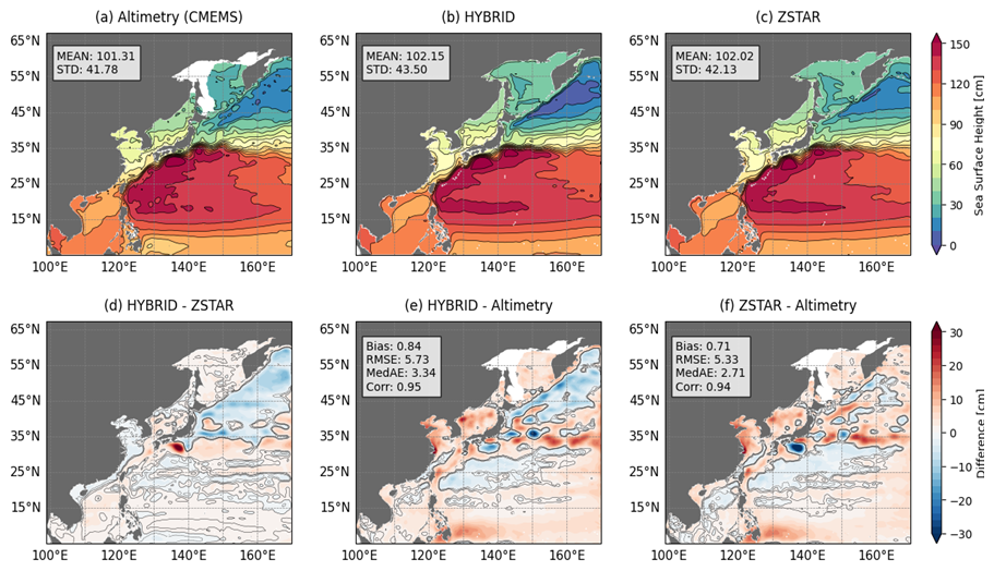
Figure 7 Mean sea surface height (SSH) distributions from Altimetry data and HYBRID and ZSTAR simulations. (a–c) Spatial SSH distributions with corresponding means and STD. (d) Differences between HYBRID and ZSTAR. (e, f) Biases relative to Altimetry, including Bias, RMSE, MedAE, and Corr. Contour lines in (d)–(f) indicate SSH biases ranging from −1.0 to 1.0 cm at 1.0 cm intervals.

Figure S2 in the Supplement also presents the MLD distribution for boreal summer (JJA), when the mixed layer is generally shallower due to enhanced stratification. The estimated summer MLD was shallow across most of the domain (mean: 19.15 m), deepening in western boundary current regions. HYBRID underestimated the MLD (mean: 17.21 m), while ZSTAR slightly overestimated it. ZSTAR showed a higher spatial correlation with the observation and along with lower RMSE.

3.2 Upper-ocean circulation and variability

To ensure a consistent reference level when comparing SSH between the models and the Altimetry dataset, the mean absolute difference between each model and Altimetry SSH was subtracted from the respective model outputs. Overall, both the HYBRID and ZSTAR configurations exhibited SSH distributions that closely aligned with Altimetry, effectively capturing the large-scale features of the region (Fig. 7). The standard deviation values of SSH variability, representing spatial gradients, were 43.50 cm for HYBRID and 42.13 cm for ZSTAR, compared to 41.78 cm for Altimetry. These values indicate that both configurations reproduced SSH gradients well, with HYBRID exhibiting slightly larger spatial variability than ZSTAR. Both configurations showed similar SSH biases, with an overall underestimation south of Japan, where Kuroshio recirculation occurs. The spatial correlation coefficients for both HYBRID and ZSTAR indicate strong agreement with the reference dataset.

As described by Qiu (2023) and Chang et al. (2024), SSH variability can be divided into large-scale and mesoscale components. This classification was based on a frequency spectrum analysis of Altimetry data, which revealed prominent peaks at both high and low frequencies, with a sharp decline to near zero at approximately two years. Accordingly, applying low-pass and high-pass filters allows for the separation of these components, effectively distinguishing large-scale ocean circulation, which evolves over interannual to decadal timescales, from high-frequency mesoscale eddy variability, which is characterized by shorter-lived fluctuations such as eddies and meanders.

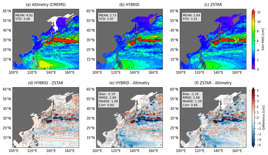
Figure 8 Root-mean-square (RMS) sea surface height (SSH) variability from low-pass filtered Altimetry data and HYBRID and ZSTAR simulations. (a–c) Spatial RMS SSH distributions with corresponding means and STD. (d) Differences between HYBRID and ZSTAR. (e, f) Biases relative to Altimetry, including Bias, RMSE, MedAE, and Corr. Contour lines in (d)–(f) indicate RMS SSH biases ranging from −1.0 to 1.0 cm at 1.0 cm intervals.

Figure 8 compares the large-scale SSH variability of the HYBRID and ZSTAR configurations with Altimetry after applying a 2 year low-pass filter. The root-mean-square (RMS) SSH variability was 2.73 cm for HYBRID and 2.69 cm for ZSTAR, both lower than the Altimetry reference value of 4.92 cm. The standard deviations for HYBRID and ZSTAR similarly indicated reduced variability compared to Altimetry, which had a standard deviation of 3.48 cm. Both models underestimated large-scale variability in key dynamic regions, including the North Equatorial Current, Kuroshio Current, and Kuroshio Extension. In particular, HYBRID exhibited a pronounced underestimation in the Kuroshio Extension region while overestimating variability in the Kuroshio Recirculation area and the East/Japan Sea. In terms of spatial correlation, ZSTAR achieved a higher correlation coefficient (0.66) with Altimetry than HYBRID (0.60), indicating better spatial agreement in large-scale variability patterns.

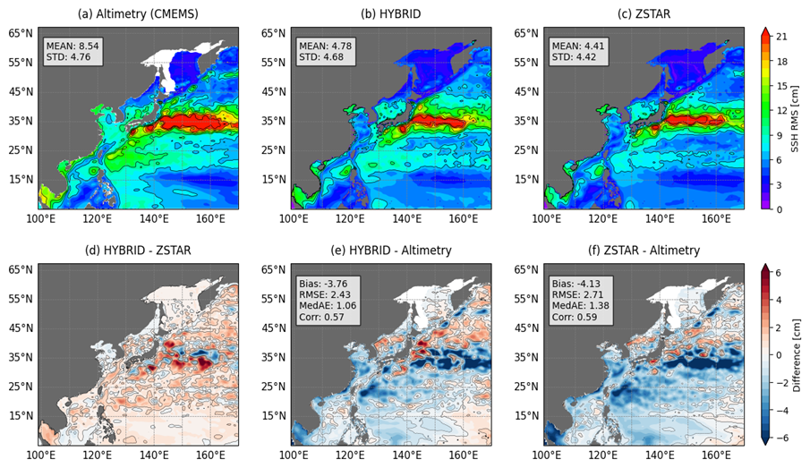
Figure 9 Root-mean-square (RMS) sea surface height (SSH) variability from high-pass filtered Altimetry data and HYBRID and ZSTAR simulations. (a–c) Spatial RMS SSH distributions with corresponding means and STD. (d) Differences between HYBRID and ZSTAR. (e, f) Biases relative to Altimetry, including Bias, RMSE, MedAE, and Corr. Contour lines in (d)–(f) indicate RMS SSH biases ranging from −1.0 to 1.0 cm at 1.0 cm intervals.

Figure 9 illustrates the mesoscale variability of SSH after applying a high-pass filter, which extracts the high-frequency components associated with mesoscale eddies and smaller-scale oceanographic features. The mean RMS SSH variability was 4.78 cm for HYBRID and 4.41 cm for ZSTAR, both significantly lower than the Altimetry reference value of 8.54 cm. Similarly, the standard deviations for HYBRID (4.68 cm) and ZSTAR (4.42 cm) were lower than those of Altimetry (4.76 cm). The discrepancies between both configurations and Altimetry were further reflected in the bias and RMSE values. HYBRID exhibited a bias of −3.76 cm and an RMSE of 2.43 cm, while ZSTAR had a bias of −4.05 cm and an RMSE of 2.64 cm. ZSTAR underestimated mesoscale variability in the open ocean of the NWP, whereas HYBRID showed a more pronounced underestimation in the Kuroshio and its Extension compared to ZSTAR. Additionally, both configurations had low spatial correlations with Altimetry, with HYBRID achieving a correlation of 0.57 and ZSTAR a slightly higher correlation of 0.59. These results suggest that while both configurations captured some aspects of mesoscale variability, they tended to underestimate its intensity and struggled to fully resolve the finer-scale structures observed in the Altimetry data.

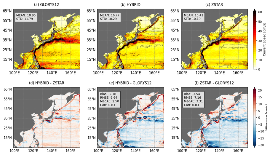
Figure 10 Mean surface current speed from GLORYS12, HYBRID, and ZSTAR simulations. (a–c) Spatial distributions of surface current speed with corresponding means and STD. (d) Differences between HYBRID and ZSTAR. (e, f) Biases relative to GLORYS12, including Bias, RMSE, MedAE, and Corr.

Figure 10 compares the surface current speeds of the HYBRID and ZSTAR configurations with the GLORYS12 reanalysis. Both models effectively captured the complex ocean current systems in the NWP, including key currents such as the Kuroshio, Oyashio, and North Equatorial Current. However, both configurations tended to underestimate current speeds in regions influenced by these currents. Specifically, in areas such as the Kuroshio and its extension, the Subtropical Counter Current, the North Equatorial Current, and the South China Sea, both models underestimated current speeds compared to GLORYS12. In contrast, both configurations overestimated current speeds in the East/Japan Sea. Both HYBRID and ZSTAR underestimated current speeds, as reflected in their bias and RMSE values. HYBRID exhibited a bias of −2.18 cm s⁻¹ and an RMSE of 6.64 cm s⁻¹, while ZSTAR showed a slightly larger bias of −3.54 cm s⁻¹ and an RMSE of 7.16 cm s⁻¹. The correlation with respect to GLORYS12 was high for both configurations, indicating good overall agreement in capturing large-scale current patterns.

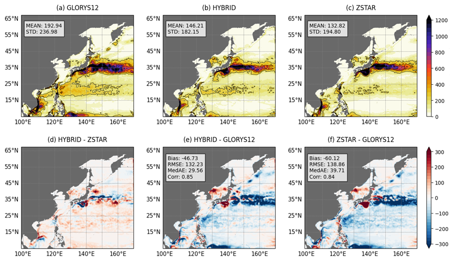
Figure 11 Mean eddy kinetic energy (EKE) from GLORYS12, HYBRID, and ZSTAR simulations. (a–c) Spatial EKE distributions with corresponding means and STD. (d) Differences between HYBRID and ZSTAR. (e, f) Biases relative to GLORYS12, including Bias, RMSE, MedAE, and Corr.

A comparison of the EKE between the HYBRID and ZSTAR configurations and GLORYS12 showed that both configurations exhibited high spatial correlation with GLORYS12, successfully capturing the general EKE distribution (Fig. 11). However, both models tended to underestimate EKE across most regions, with mean biases of −46.73 cm² s⁻² for HYBRID and −60.12 cm² s⁻² for ZSTAR. Specifically, both configurations underestimated EKE in the southern boundary regions, the Subtropical Counter Current region, and the Kuroshio and its extension, while overestimating EKE in the Kuroshio recirculation region and the East/Japan Sea. ZSTAR underestimated EKE in the open ocean of the NWP but overestimated it in the Kuroshio recirculation region and the East/Japan Sea, consistent with its higher bias in these areas. In contrast, HYBRID exhibited a more significant underestimation of EKE in the Kuroshio and its extension region compared to ZSTAR. Additionally, the MedAE was 29.56 cm² s⁻² for HYBRID and 39.71 cm² s⁻² for ZSTAR, suggesting that HYBRID performed slightly better in capturing the magnitude of EKE variability across the domain.

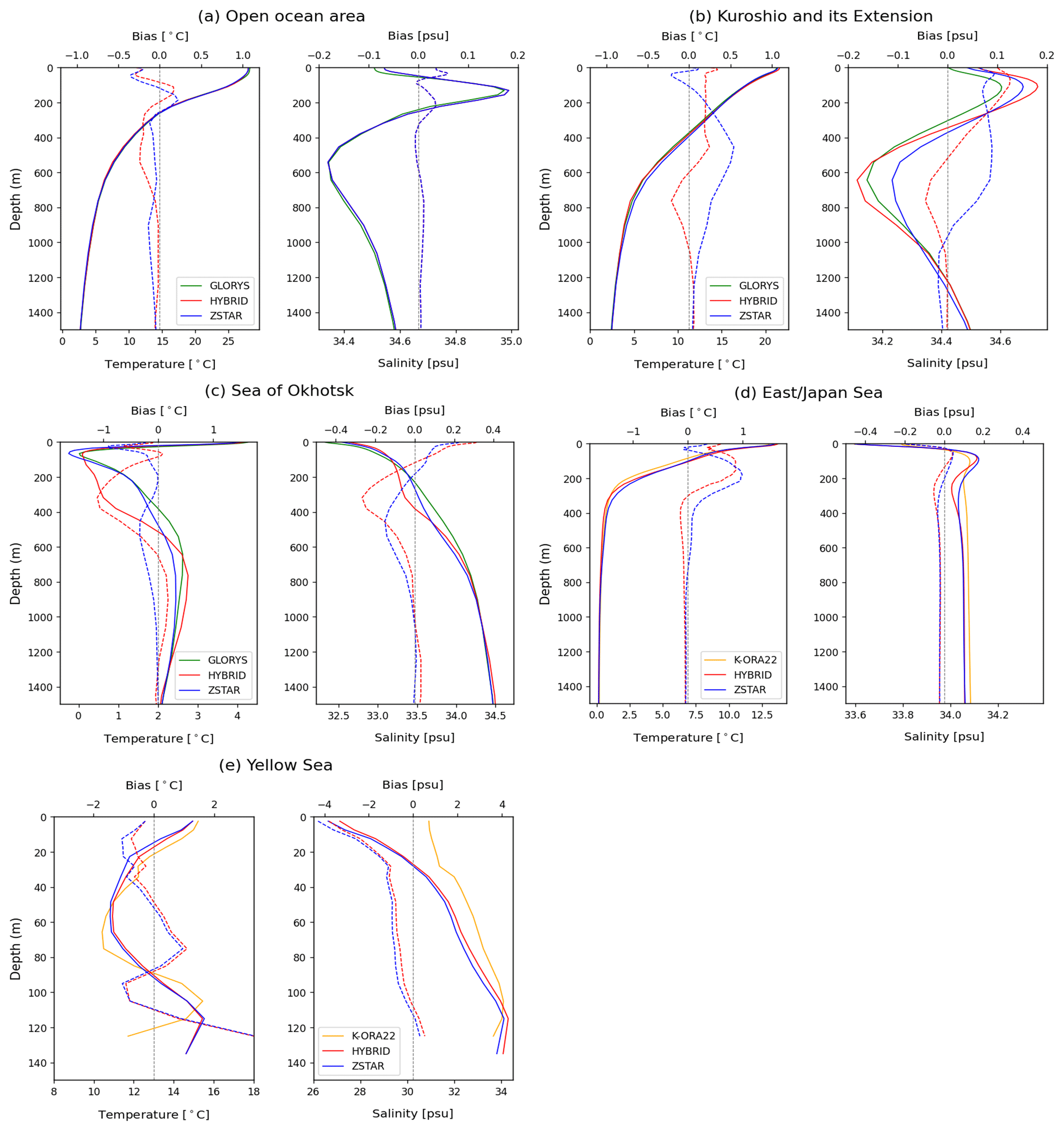
Figure 12 Vertical mean profiles of temperature (left) and salinity (right) from GLORYS12 (green), K-ORA22 (orange), HYBRID (red), and ZSTAR (blue) across different Northwest Pacific (NWP) regions: (a) Open ocean area, (b) Kuroshio and its Extension, (c) Sea of Okhotsk, (d) East/Japan Sea, and (e) Yellow Sea. Biases for HYBRID (red dashed lines) and ZSTAR (blue dashed lines) are shown relative to the reference datasets (GLORYS12 or K-ORA22).

3.3 Vertical structure and water masses

The vertical profiles of temperature and salinity biases for the HYBRID and ZSTAR configurations were compared against GLORYS12 and K-ORA22 across different regions in the NWP (Fig. 12). In the open ocean of the NWP (Fig. 12a), both configurations exhibited low biases and closely followed the vertical structures of temperature and salinity observed in GLORYS12. However, in the Kuroshio and its extension (Fig. 12b), the bias patterns differed between the two configurations. ZSTAR showed lower temperature and salinity biases up to 200 m compared to HYBRID, whereas HYBRID better maintained the vertical structure of GLORYS12 below 200 m, with temperature biases remaining below 0.3 °C and salinity biases under 0.05 psu.

In the Sea of Okhotsk (Fig. 12c), HYBRID exhibited larger negative biases than ZSTAR between 100 and 600 m, with a temperature bias of approximately −1 °C at 400 m. The salinity bias for HYBRID was also more pronounced, reaching around −0.3 psu at 400 m, whereas ZSTAR showed relatively lower biases. In the East/Japan Sea (Fig. 12d), both models simulated salinity patterns similar to K-ORA22, but ZSTAR exhibited a greater temperature bias of approximately 1 °C below 200 m than HYBRID. In the Yellow Sea (Fig. 12e), both models displayed similar temperature and salinity profiles. The Yellow Sea is characterized by the Yellow Sea Bottom Cold Water Mass (YBCWM), a cold and dense water mass that forms near the bottom. However, both configurations showed positive temperature biases exceeding 2 °C near the bottom, suggesting limitations in accurately representing YBCWM. For salinity, both models exhibited large negative biases at the surface, with HYBRID and ZSTAR showing deviations of approximately −4 psu. This suggests that the river discharge forcing applied in both models overestimated freshwater input from major rivers in the region, such as the Yangtze and Yellow Rivers.

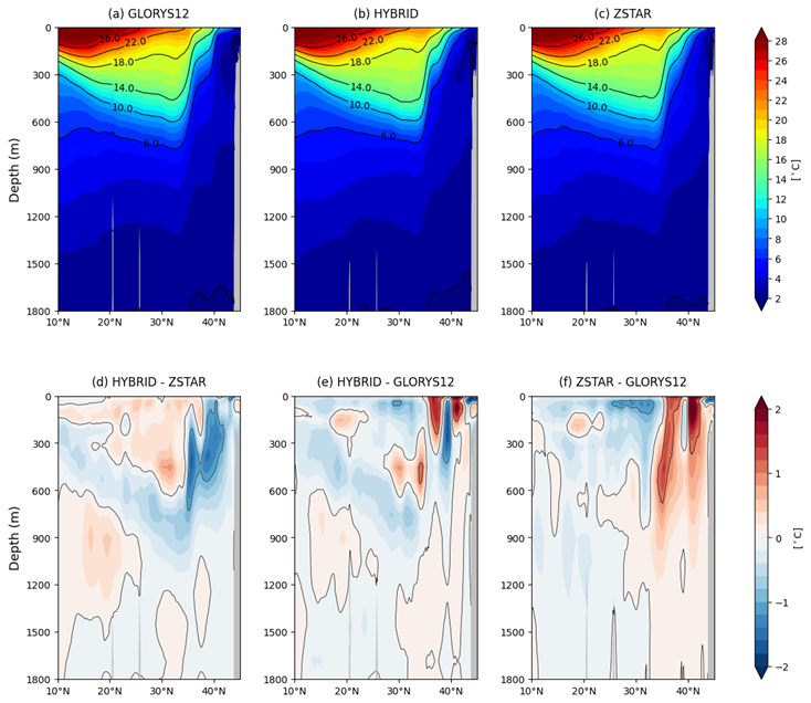
Figure 13 Meridional temperature section along 148° E from (a) GLORYS12 reanalysis, (b) HYBRID simulation, and (c) ZSTAR simulation, showing vertical temperature distribution. Panels (d–f) illustrate temperature differences: HYBRID vs. ZSTAR (d), HYBRID vs. GLORYS12 (e), and ZSTAR vs. GLORYS12 (f). Contour lines in (d)–(f) indicate temperature biases ranging from −1.0 to 1.0 °C at 1.0 °C intervals.

The NWP is characterized by two distinct water masses: Subtropical Mode Water (STMW) and North Pacific Intermediate Water (NPIW), both of which play crucial roles in the region's physical and biogeochemical processes. STMW is typically found within the upper thermocline at depths of 100–300 m, while NPIW occupies the intermediate layer, extending from approximately 300 to 800 m.

Figure 13 presents a comparison of the vertical temperature section along 148° E for HYBRID and ZSTAR against GLORYS12. Both configurations reproduced an overall temperature structure similar to that of GLORYS12, effectively capturing the vertical thermal structure. However, ZSTAR exhibited a positive temperature bias exceeding 1 °C in high-latitude regions.

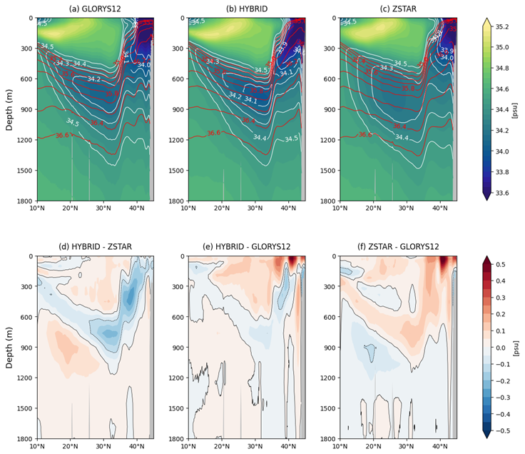
Figure 14 Meridional salinity section along 148° E from (a) GLORYS12 reanalysis, (b) HYBRID simulation, and (c) ZSTAR simulation, showing vertical salinity distribution. Panels (d–f) display salinity differences: HYBRID vs. ZSTAR (d), HYBRID vs. GLORYS12 (e), and ZSTAR vs. GLORYS12 (f). Red contour lines in (a)–(c) indicate σ2 (density referenced to 2000 dbar) for each dataset. Contour lines in (d)–(f) represent salinity biases ranging from −0.1 to 0.1 psu at 0.1 psu intervals.

Figure 14 compares the vertical salinity section along 148° E between HYBRID, ZSTAR, and GLORYS12. HYBRID closely reproduced the NPIW salinity structure, while ZSTAR exhibited a salinity bias of approximately 0.3 psu, indicating challenges in accurately representing NPIW. When examining σ2 (density referenced to 2000 dbar) within the range of 35.0 to 36.6, HYBRID accurately captured the thickness of the σ2 layer associated with NPIW, whereas ZSTAR tended to overestimate its thickness. However, both configurations showed a positive salinity bias of approximately 0.3 psu in STMW, suggesting a slight overestimation of salinity in this region.

The σ2 value of 35.8 is defined as the salinity minimum layer of NPIW, and the depth at which this minimum layer is located was extracted from each dataset. The temperature and salinity values at this depth from both configurations were then compared with those obtained from GLORYS12.

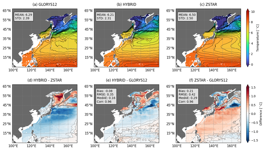
Figure 15 Temperature distributions at depths corresponding to σ2 = 35.8 from (a) GLORYS12, (b) HYBRID, and (c) ZSTAR simulations, along with their respective means and STD. (d) Differences between HYBRID and ZSTAR. (e, f) Biases relative to GLORYS12, including Bias, RMSE, MedAE, and Corr. Contour lines in (d)–(f) indicate temperature biases ranging from −0.1 to 0.1 °C at 0.1 °C intervals.

Figure 15 compares the temperature at the depth of the salinity minimum layer for both configurations against GLORYS12. HYBRID generally exhibited a spatial temperature distribution similar to GLORYS12, except for a positive temperature bias exceeding 1 °C in the OKH region. In contrast, ZSTAR tended to exhibit a positive bias across most regions, except for areas influenced by open boundaries. Notably, ZSTAR exhibited a temperature bias of approximately 1 °C in the transition zone where the Kuroshio and Oyashio currents converge, a critical region for NPIW formation.

The salinity distribution at depths, where the salinity minimum layer is located was also compared between HYBRID and ZSTAR relative to the GLORYS12 (Fig. S3 in the Supplement). In most regions, HYBRID showed minimal salinity biases relative to GLORYS12, except for the OKH region, where it exhibited a positive salinity bias. In contrast, ZSTAR showed a salinity bias of approximately 0.2 psu, except for areas influenced by open boundaries.

These results indicate that ZSTAR exhibited more significant positive temperature and salinity biases at depths where the minimum salinity layer is present compared to HYBRID. The larger biases observed in ZSTAR at intermediate depths are likely attributable to spurious diapycnal mixing, a well-known issue in ZSTAR configurations (Griffies et al., 2000). This excessive mixing can lead to artificial erosion of water mass properties, reducing the sharpness of the salinity minimum layer and contributing to the observed biases.

To further investigate the differences in vertical structure and water mass representation between the HYBRID and ZSTAR configurations, an idealized age tracer experiment was conducted following the spin-up simulation. This experiment was performed over a 10 year integration period to assess ventilation and subduction processes in both configurations. To facilitate comparison, the age tracer values were normalized following the approach of Adcroft et al. (2019). A value of 0 represents older water that has remained in the interior for an extended period, while a value of 1 indicates younger water that has been more recently ventilated from the surface.

In high-latitude regions where ZSTAR exhibited positive temperature and salinity biases, the normalized age values were lower in ZSTAR compared to HYBRID, indicating the presence of older water. At depths associated with NPIW formation, ZSTAR showed higher normalized age values than HYBRID, meaning it simulated younger water in this critical layer. These patterns suggest that spurious diapycnal mixing – a known issue in traditional Eulerian geopotential coordinate models – plays a significant role in ZSTAR. In high-latitude regions, stronger diapycnal mixing in ZSTAR allows older water from deeper layers to diffuse upward, leading to the observed positive temperature and salinity biases (Figs. 13f and 14f). Conversely, at NPIW depths, enhanced diapycnal mixing in ZSTAR facilitates the downward diffusion of young surface water, disrupting the natural vertical separation of water masses and eroding the salinity minimum layer. While HYBRID preserved vertical water mass properties more effectively, spurious diapycnal mixing in ZSTAR reduced its ability to accurately simulate intermediate water properties, particularly in regions critical for NPIW formation (Figs. 14 and S3).

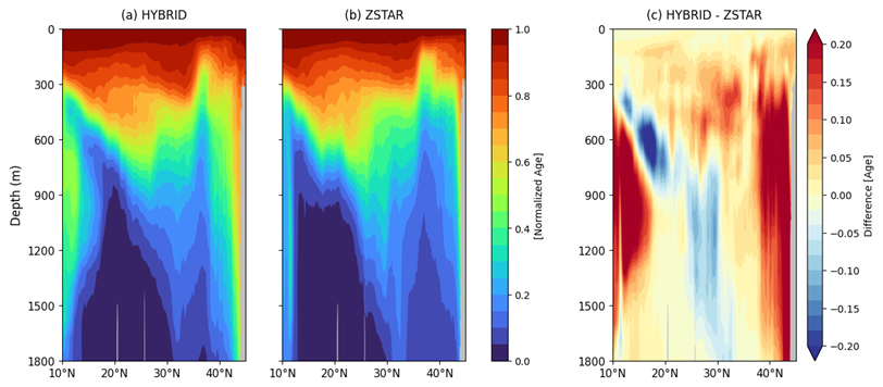
Figure 16 Meridional normalized age tracer along 148° E for (a) HYBRID, (b) ZSTAR, and (c) their difference (HYBRID – ZSTAR). The normalized age is computed as $f=(A_{\text{max}}-A)/A_{\text{max}}$, where A_max is the maximum age in the simulation, following Adcroft et al. (2019). Values range from 0 (oldest water) to 1 (youngest water), representing the relative ventilation age of water masses.

In the Yellow Sea, the YBCWM is a distinct water mass that plays a crucial role in shaping regional hydrography and seasonal dynamics. It primarily forms in winter, when surface cooling induces vertical convection, allowing cold, dense water to accumulate in the deeper regions of the Yellow Sea. As spring and summer progress, surface warming enhances stratification, effectively trapping the YBCWM at the subsurface. Accurate representation of the YBCWM is critical, as it influences regional circulation, water mass transformation, and broader atmospheric and biogeochemical processes. The presence of the YBCWM modulates ocean-atmosphere interactions, potentially impacting typhoon intensification over the Yellow Sea basin (Moon and Kwon, 2012). Additionally, it plays a key role in regulating nutrient availability, oxygen dynamics, and primary production, thereby shaping regional biogeochemical cycling and ecosystem productivity (Huo et al., 2012; Su et al., 2013).

Figure 17 presents the bottom temperature distribution during summer and its bias relative to the K-ORA22 reanalysis. Since GLORYS12 fails to represent the YBCWM entirely (Chang et al., 2024), K-ORA22 was used as the reference dataset for comparison. The YBCWM in summer is generally characterized by a circular water mass enclosed by the 10 °C isotherm near the bottom (Zhang et al., 2008; Li et al., 2021). This structure was well captured in K-ORA22, and both the HYBRID and ZSTAR configurations successfully reproduced its overall pattern.

However, as shown in Fig. 11e, both configurations exhibited a warm bias of approximately 2 °C at the bottom compared to K-ORA22, with the bias being more pronounced in ZSTAR. Additionally, the YBCWM was shifted westward, resulting in a cold bias on the western side. Despite these biases, it is notable that both configurations successfully simulated the YBCWM without data assimilation – a significant improvement, as previous models have often failed to reproduce this feature due to the absence of explicit tidal forcing and reliance on parameterized tidal mixing.

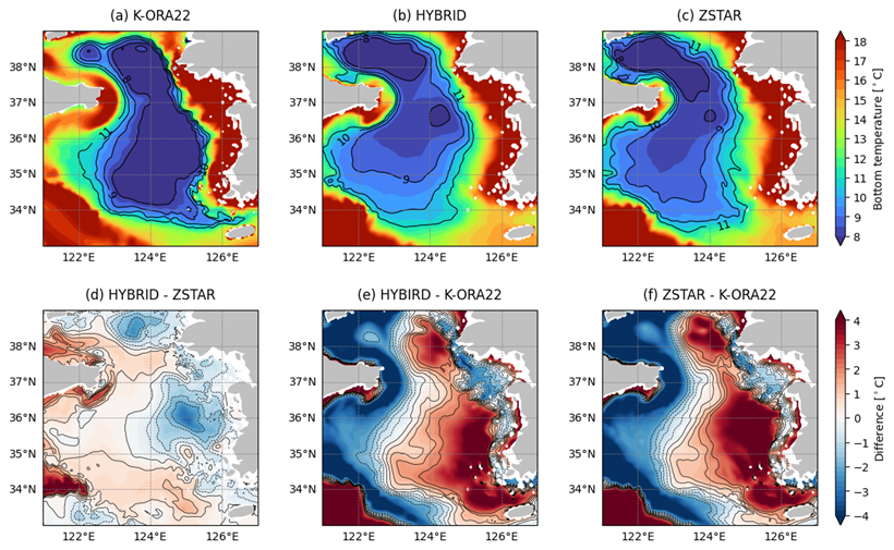
Figure 17 Bottom temperature distributions in the Yellow Sea from (a) K-ORA22, (b) HYBRID, and (c) ZSTAR simulations. (d) Temperature difference between HYBRID and ZSTAR. (e, f) Biases relative to K-ORA22. Contour lines in (d)–(f) indicate temperature biases ranging from −2.0 to 2.0 °C at 0.5 °C intervals.

3.4 Volume transport

The volume transport through key straits in the Northwest Pacific (NWP) was analysed to evaluate the performance of the HYBRID and ZSTAR configurations (Fig. 18). The Tokara Strait serves as a crucial passage for the Kuroshio Current, making it a key indicator of the current's transport dynamics. Meanwhile, the Korea/Tsushima Strait, Tsugaru Strait, and Soya Strait play significant roles in regulating the inflow and outflow of heat and salt from lower latitudes into the East/Japan Sea and their subsequent exchange with the open ocean. Given the limited availability of direct observational data for these straits, observed climatology or long-term mean values from previous studies were used for comparison.

In the Tokara Strait, the observed annual mean volume transport from 1987 to 2010 was 21.39 Sv (Wei et al., 2013). Both configurations overestimated this transport, with HYBRID simulating an annual mean of 28.39 Sv (overestimating by 7.01 Sv) and ZSTAR simulating 27.15 Sv (overestimating by 5.76 Sv). The transport magnitude was consistently higher in HYBRID than in ZSTAR.

For the Korea/Tsushima Strait, the observed annual mean transport, derived from sea-level differences (Shin et al., 2022), was 2.61 Sv. HYBRID simulated a higher transport of 2.72 Sv, exceeding the observed value by 0.11 Sv, while ZSTAR underestimated it with an annual mean of 2.48 Sv, showing a negative bias of 0.13 Sv.

According to acoustic Doppler current profiler measurements from 2003 to 2007, the mean volume transport through the Tsugaru Strait was 1.47 Sv (Han et al., 2016), consistent with previous estimates of approximately 1.50 Sv (Na et al., 2009; Ohshima and Kuga, 2023). Both configurations overestimated this value, with HYBRID predicting an annual mean transport of 2.38 Sv and ZSTAR predicting 2.04 Sv.

In the Soya Strait, the observed annual mean transport, estimated from high-frequency radar observations between 2003 and 2015 (Ohshima and Kuga, 2023), was 0.90 Sv. Both configurations underestimated the transport, with HYBRID simulating 0.47 Sv and ZSTAR showing 0.56 Sv.

Overall, the HYBRID configuration tended to overestimate transport, particularly through the Tokara and Tsugaru Straits, while underestimating it in the Soya Strait. In contrast, ZSTAR generally underestimated transport, as observed in the Korea/Tsushima Strait and Soya Straits.

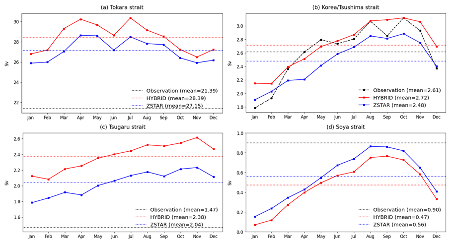
Figure 18 Monthly climatological mean volume transport at (a) Tokara Strait, (b) Korea/Tsushima Strait, (c) Tsugaru Strait, and (d) Soya Strait. Observations (black) are compared with HYBRID (red) and ZSTAR (blue). Dotted lines represent the annual mean for each dataset, while solid lines show the monthly climatological mean.

3.5 Tide simulation

Tides play a crucial role in shaping ocean dynamics in the NWP, where tidal forces strongly influence circulation, mixing, and water mass distribution. This is particularly evident in the Yellow Sea, which is characterized by exceptionally large tidal amplitudes, with a tidal range exceeding 8 m. Given the significant impact of tides on the physical and biogeochemical characteristics of this region, it is essential to assess the performance of tidal representations in these configurations.

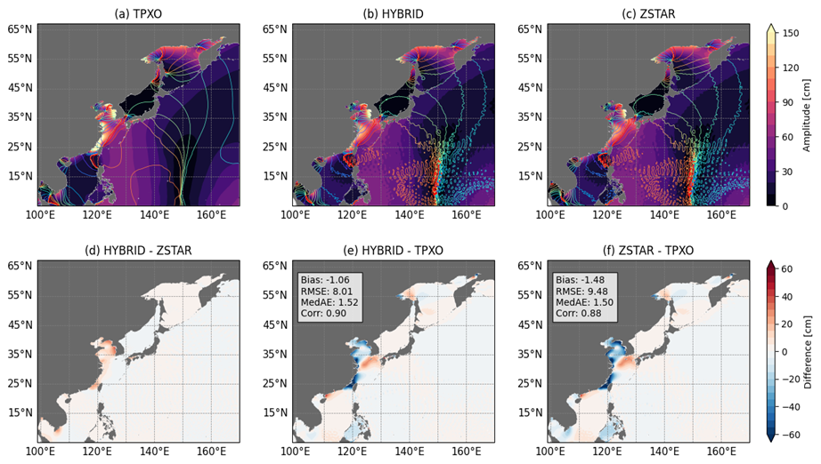
Figure 19 Semidiurnal M2 tidal amplitude and phase from TPXO data, HYBRID, and ZSTAR simulations. Shaded contours represent tidal amplitude, while overlaid coloured contours show tidal phase for M2 (a–c). Panels below display tidal amplitude differences: (a) HYBRID vs. ZSTAR, (b) HYBRID vs. TPXO, and (c) ZSTAR vs. TPXO. Metrics include Bias, RMSE, MedAE, and Corr.

Figure 19 compares the tidal amplitude and phase of the semidiurnal M2 component between the HYBRID and ZSTAR configurations using TPXO, which served as the tidal boundary forcing dataset. Both configurations accurately simulated the tidal amplitude and phase, with HYBRID achieving a spatial correlation of 0.90 and ZSTAR showing 0.88, indicating a strong representation of tidal characteristics in the region. However, both models underestimated the M2 amplitude along the southeastern coast of China and in the Yellow Sea, while overestimating it in the Korea/Tsushima Strait. Notably, ZSTAR exhibited a more pronounced underestimation of the M2 amplitude than HYBRID in these regions.

Both configurations effectively simulated the K1 tidal amplitude and phase, with a high spatial correlation of 0.94 against TPXO data (Fig. S3). However, both models underestimated the K1 amplitude in the Yellow Sea, with a stronger bias in ZSTAR. In the Sea of Okhotsk coastal region, HYBRID overestimated the amplitude, whereas ZSTAR showed a mixed bias, overestimating in the west and underestimating in the east, reflecting regional differences in tidal representation.

Overall, both configurations performed well in reproducing the amplitude and phase of the semidiurnal and diurnal tidal components. Nevertheless, the consistent underestimation of the Yellow Sea tidal amplitude across both configurations highlighted a common limitation. Importantly, the results suggested that tidal representation was influenced by the vertical coordinate system, with HYBRID showing better agreement with TPXO tidal amplitudes than ZSTAR. This suggests that HYBRID may offer advantages in improving tidal simulations, particularly in regions with complex bathymetry and strong tidal forcing.

3.6 Computational cost

Compared with the previous MOM5-based regional model described in Jin et al. (2024), MOM6 demonstrated noticeably higher computational efficiency, primarily due to improvements in numerical stability that allow longer stable timesteps. Specifically, the maximum baroclinic timestep increased from 150 s in MOM5 to 300 s in MOM6, and the tracer timestep increased from 300 s in MOM5 to 900 s in MOM6, substantially reducing the total number of integration steps required for a given simulation period. This enhancement in numerical stability directly translates into greater computational efficiency under the same model resolution.

To further assess how the choice of vertical coordinate system influences computational cost within MOM6, we compared the HYBRID and ZSTAR configurations using the same supercomputer node and identical processor layouts (42 × 40 PE decomposition, with 536 PEs masked through land processor masking). The ZSTAR configuration required an average of 23 h per simulated year, whereas HYBRID completed the same simulation in 20.2 h, indicating that ZSTAR consumed approximately 2 h more. This difference primarily reflects the number of active vertical layers in each configuration: ZSTAR maintained a consistently high number of layers across most of the domain, while HYBRID adaptively reduced active layers in weakly stratified and shallow regions (Fig. S5 in the Supplement), leading to fewer computations

4 Discussion

In this study, we updated the base model of KOOS-OPEM, which had been developed using previous versions of the MOM series, to MOM6 to enhance regional ocean modeling capabilities. MOM6 introduced significant improvements in computational efficiency, numerical stability, and flexibility in vertical coordinate selection, enabling a more advanced representation of oceanic processes (Jackson et al., 2008; Reichl and Hallberg, 2018; Reichl and Li, 2019; Adcroft et al., 2019; Griffies et al., 2020). Given the increasing demand for accurate ocean predictions in the NWP and its marginal seas under a changing climate, this update aimed to improve the model's ability to represent key oceanic physical dynamics, current systems, and the physical characteristics of major marginal seas. Comprehensive sensitivity experiments were conducted to evaluate performance differences between the ZSTAR coordinate system, used in previous models, and the HYBRID system within MOM6's Lagrangian remapping framework. To ensure a robust assessment, both configurations were compared against multiple observational datasets and two reanalysis products, GLORYS12 and K-ORA22, providing insights into how vertical coordinate systems influence the reproduction of key physical and dynamical features of the NWP.

The results revealed significant differences between the HYBRID and ZSTAR configurations while also highlighting shared limitations in representing certain oceanographic variabilities.

A comparison of modeled SST with OISST satellite observations showed that both configurations effectively captured seasonal SST patterns and gradients, demonstrating strong agreement with the OISST dataset (Figs. 3 and 4). However, both exhibited warm biases during winter, particularly in the Kuroshio and its extension and East/Japan sea. These SST biases may partly stem from the relatively coarse vertical resolution near the surface, where the uppermost layer thickness of 2 m in the ZSTAR grid (and similarly in HYBRID) can limit representation of diurnal SST variability (Bernie et al., 2005; Siddorn and Furner, 2013). Such resolution may underestimate sub-daily mixing and surface heat exchange, contributing to persistent warm biases under strong insolation conditions. Future sensitivity experiments with finer near-surface resolution (e.g., 1 m thickness for the upper layers) are planned to evaluate whether enhancing vertical discretization can mitigate these SST biases.

Beyond the SST biases, both configurations exhibited noticeable differences in wintertime MLD, particularly south of the Kuroshio Extension and in the Okhotsk Sea (Fig. 6). In the Kuroshio region (25–35° N), both configurations captured strong stratification beneath the mixed layer, but the vertical structure differed. HYBRID exhibited stronger stratification slightly deeper (below ∼ 100 m) from late summer to early winter, while ZSTAR showed stronger stratification just below the mixed layer (around 50–100 m) (Fig. S6 in the Supplement). The deeper stratification maximum in HYBRID stabilized the upper ocean and limited wintertime convective deepening, resulting in a shallower and more realistic MLD compared to ZSTAR, which tended to overestimate MLDs due to weaker near-surface stratification. In the Sea of Okhotsk, MLD differences mainly arose from the vertical layer representation: the σ2-based HYBRID coordinate formed thicker layers in weakly stratified waters (Fig. S7 in the Supplement), reducing vertical resolution below approximately 80–200 m and leading to slightly deeper MLDs than ZSTAR. These results suggest that the way each vertical coordinate system represents stratification strength and layer spacing substantially influences the simulated MLD structure across the Northwest Pacific.

The evaluation of vertical temperature and salinity structures provided further insights into differences between HYBRID and ZSTAR. Across most regions, both configurations successfully reproduced vertical hydrographic properties comparable to those in reanalysis datasets. However, notable discrepancies emerged in their representation of specific water masses.

The NPIW was represented more accurately in HYBRID than in ZSTAR. HYBRID closely captured the thickness and vertical structure of the isopycnal layer associated with NPIW (Fig. 14) and exhibited lower salinity biases compared to GLORYS12. In contrast, ZSTAR overestimated the thickness of the σ2 layer associated with NPIW and showed a salinity bias of approximately 0.2 psu. These differences were attributed to spurious diapycnal mixing inherent in the traditional ZSTAR system, which disrupted stratification and reduced the accuracy of intermediate water properties.

The idealized age tracer experiment further clarified these discrepancies (Fig. 16). At depths associated with NPIW formation, ZSTAR exhibited higher normalized age values than HYBRID, indicating the simulation of younger water masses in these layers. This suggested that enhanced diapycnal mixing in ZSTAR facilitated downward diffusion of younger surface waters, eroding the salinity minimum layer that defines NPIW. In contrast, HYBRID preserved vertical stratification, leading to a more accurate representation of NPIW.

However, HYBRID exhibited poorer performance than ZSTAR in high-latitude regions, as indicated by larger temperature and salinity biases between depths of 100 and 600 m (Fig. 12c). This discrepancy was primarily due to a common limitation of isopycnal coordinates: poor vertical resolution in weakly stratified regions, which are characteristic of high latitudes (Adcroft et al., 2019). A comparison of active layers between HYBRID and ZSTAR (Figs. S4 and S7 in the Supplement) revealed that HYBRID generally maintained fewer active layers, particularly in weakly stratified regions. This reduction in active layers likely contributed to the increased temperature and salinity biases observed in HYBRID, underscoring the challenges of using isopycnal coordinates in high-latitude environments.

To improve water property representation in these regions, adjustments to the maximum layer thickness or modifications to the target density profile could enhance vertical resolution and better capture stratification. Such refinements may mitigate resolution loss and reduce temperature and salinity biases in HYBRID.

Both configurations successfully reproduced the overall structure of the YBCWM despite the absence of data assimilation (Fig. 17). However, notable differences were observed, with HYBRID demonstrating a more accurate representation of temperature structure than ZSTAR. This improvement was closely linked to HYBRID's better representation of seasonal stratification. A well-defined seasonal stratification is crucial for YBCWM formation, as it reduces excessive vertical mixing in summer and allows cold water to persist near the bottom. Given the sensitivity of YBCWM formation to vertical mixing, understanding the mechanisms governing stratification is essential for improving its representation in ocean models.

To further investigate the processes influencing its formation, sensitivity experiments conducted with and without the shear-driven mixing parameterization (Jackson et al., 2008) revealed that this parameterization played a crucial role in shaping and maintaining the YBCWM (not shown here). However, despite its effectiveness in reproducing the YBCWM structure, the shear-driven mixing parameterization (Jackson et al., 2008) tended to induce excessive mixing in certain shelf regions with strong tidal forcing (Drenkard et al., 2025). Therefore, future work should focus on optimizing the turbulent decay length scale in the Jackson parameterization to better regulate mixing intensity in these regions (Drenkard et al., 2025).

Building on these findings, the evaluation of tidal dynamics further highlighted differences between the HYBRID and ZSTAR configurations. Both effectively simulated the semidiurnal (M2) and diurnal (K1) tidal amplitudes and phases across the NWP, demonstrating their ability to reproduce key tidal characteristics. However, HYBRID outperformed ZSTAR in capturing the barotropic tidal amplitude in the Yellow Sea, particularly for the M2 tide. Several studies have emphasized that barotropic tides in this region are seasonally modulated by stratification through its influence on bottom friction and energy dissipation (e.g., Kang et al., 2002; Müller et al., 2014). A comparison of the YBCWM further supports the differences in stratification representation between the two configurations. HYBRID exhibited a lower temperature bias near the bottom compared to ZSTAR, suggesting that it better captured seasonal stratification in the Yellow Sea. Since seasonal stratification directly influences both YBCWM formation and internal tide modulation, HYBRID's improved tidal amplitude simulation is likely linked to its enhanced representation of stratification. Given the strong dependence of baroclinic tides on stratification and vertical mixing, the choice of vertical coordinate system plays a crucial role in accurately capturing these processes. While HYBRID demonstrated improved tidal amplitude reproduction in the Yellow Sea, further investigation is needed to clarify the mechanisms through which different vertical coordinates influence tidal dynamics, particularly the generation, propagation, and dissipation of baroclinic tides.

Both configurations showed noticeable differences in volume transport through major straits of the Northwest Pacific. HYBRID tended to overestimate transport through the Tokara and Tsugaru Straits, whereas ZSTAR underestimated it in the Korea/Tsushima. Since both used identical bottom drag and free-slip boundary conditions, these differences are unlikely to result from frictional effects. Instead, the stronger stratification and steeper isopycnal slopes represented by HYBRID (Figs. S8 and S9 in the Supplement) may enhance the baroclinic pressure-gradient force and lead to larger transports. However, further investigation is needed to clarify the mechanisms through which different vertical coordinate systems influence transport variability in narrow straits.

Both HYBRID and ZSTAR struggled to accurately represent sea surface salinity, particularly in areas affected by river discharge (Figs. 5 and 6). Despite applying bias correction to GLOFAS, both models overestimated the freshwater influence, leading to significant negative salinity biases, exceeding −1.0 psu, in the Yellow Sea and East China Sea. To address this issue, repositioning the Yangtze River mouth further inland may better capture its interactions with the coastal ocean. Additionally, further investigation into other major rivers, such as the Yellow River, and additional bias corrections are essential to improve freshwater dynamics representation in the region.

Both configurations effectively captured the overall spatial distribution of SSH in the NWP, demonstrating strong agreement with observed large-scale patterns (Fig. 7). However, when SSH variability was analyzed separately into large-scale and mesoscale components using a 2 year cut-off period with high- and low-pass filters, both models significantly underestimated variability magnitude compared to observations. For large-scale variability (Fig. 8), the models failed to fully capture SSH variability in dynamic regions such as the Kuroshio and its extension and the North Equatorial Current. Similarly, mesoscale variability, influenced by eddies and smaller-scale processes, was also underestimated, with both configurations showing reduced intensity and weaker high-frequency fluctuations (Fig. 9). This underestimation extended to the EKE, where both HYBRID and ZSTAR failed to reproduce the observed magnitude, particularly in regions of strong mesoscale activity, such as the K-KE. While the models replicated spatial patterns and variability correlations, their inability to resolve the intensity of large- and mesoscale dynamics underscores a key limitation in accurately simulating the energetic processes defining the NWP. Addressing these limitations requires sensitivity experiments on horizontal viscosity, which plays a crucial role in modulating mesoscale and sub-mesoscale dynamics in ocean models. Excessive viscosity can overly dampen eddy activity and high-frequency fluctuations, leading to an underestimation of SSH variability and EKE, as observed in both configurations. Conversely, insufficient viscosity may introduce numerical instabilities, particularly in strong current regions such as the Kuroshio and its extension. Optimizing viscosity parameters through targeted sensitivity experiments can help balance numerical stability and realistic energy dissipation, ultimately improving the model's ability to resolve large- and mesoscale variability in the NWP.

5 Summary

The HYBRID configuration demonstrated notable advantages over ZSTAR in several key aspects of NWP simulation. It effectively captured stratification, reduced spurious diapycnal mixing, and provided more accurate representations of features such as the NPIW and tidal dynamics in the Yellow Sea. These improvements align with findings from Adcroft et al. (2019), who showed that ZSTAR induces significant warm drift in intermediate layers due to excessive diapycnal mixing, whereas HYBRID mitigates this issue by better preserving water mass properties. Given that HYBRID has proven effective not only in global ocean simulations but also in regional modeling experiments, it shows promise as a robust vertical coordinate system for high-resolution regional applications, particularly in strongly stratified environments such as the NWP. However, HYBRID also exhibited limitations, particularly in high-latitude regions where weak stratification led to significant vertical structure biases. To overcome these limitations and further optimize the HYBRID configuration, refinements in vertical resolution are necessary, particularly in weakly stratified high-latitude regions. Adjusting maximum layer thickness in these areas could help mitigate vertical resolution loss. Additionally, refining target density profiles to better capture regional stratification characteristics may enhance the model's ability to represent key water mass properties more accurately. Future work should also explore the impact of horizontal viscosity tuning to improve mesoscale energy representation and enhance eddy-driven process simulation. By addressing these issues, the HYBRID coordinate system can be further refined to provide a more robust and accurate framework for high-resolution regional ocean modeling in the NWP.

Beyond improvements in physical ocean modeling, a coupled physical-biogeochemical model is critical for a comprehensive understanding of ecosystem dynamics in the NWP. The NWP contains several ecologically significant regions, including the East/Japan Sea and Kuroshio–Oyashio Transition Zone, which support diverse marine ecosystems and essential fisheries. To fully capture these ecosystems' complexity, biogeochemical models must be integrated with physical models, allowing for a more detailed understanding of nutrient cycling, primary productivity, and ecosystem responses to environmental changes, particularly in the face of shifting climatic conditions and increasing anthropogenic pressures. Therefore, coupling COBALT with KOOS-OPEM, based on MOM6, is expected to provide a comprehensive tool for simulating both physical and biogeochemical dynamics in the NWP. This coupled system will enable more accurate predictions of key biogeochemical processes, using dynamic downscaling to assess their responses to environmental changes and long-term oceanic trends. Such efforts are crucial for advancing sustainable resource management and ensuring the long-term resilience of marine ecosystems in the NWP.