A Climate Intervention Dynamical Emulator (CIDER) for scenario space exploration

Stratospheric Aerosol Injection (SAI) is a form of proposed climate intervention to reflect incoming solar radiation, offsetting some of the impacts of greenhouse gas warming. Due to the characteristics of stratospheric circulation, the lifetime of such aerosols, and the differential impacts that different aerosol patterns can produce on surface climate, many possible scenarios of SAI implementations might exist, ranging from steady, cooperative deployments across one or more injection latitudes to highly dynamic, uncoordinated deployments involving multiple independent actors with different aims.

However, a full exploration of this scenario space is constrained by the computational cost of fully coupled climate model simulations that are usually used to evaluate the impacts of potential scenarios. Here, we describe the development and evaluation of the Climate Intervention Dynamical EmulatoR (CIDER), a climate emulator that can be used to quickly simulate the response to a SAI deployment on both a regional and a global scale for a set of variables (temperature, precipitation, evaporation, and sea ice fraction) as the injection rates vary in magnitude, latitude, and time. CIDER is trained on a large but finite set of pre-existing Earth System Model (ESM) simulations, but it can emulate novel, out-of-sample scenarios at a small fraction of a cost of one ESM simulation. Because CIDER does not include a representation of how SAI affects the diurnal and seasonal cycles, nor how it affects internal variability, it is not meant to substitute for ESMs, nor to directly inform more detailed impact analyses of SAI. Nevertheless, it can be used to quickly understand the broad impacts of different SAI strategies and produce large sets of different SAI implementations, making it a valuable tool for educational and communication purposes, for rapid identification of scenario parameters prior to simulation in a full ESM, and for coupling with Integrated Assessment Models (IAMs).

In this paper, we describe CIDER and its workflow, as well as the process we used to train on existing simulations. We then evaluate the emulator's performance on a novel scenario, simulated using the same climate model used for the training set, but not included in the set, showing that CIDER is capable of emulating outside-the-box scenarios with a high degree of fidelity. The novel scenario we use is an example of a multi-actor, uncoordinated SAI deployment, and thus rather different from the balanced, coordinated scenarios used in the training set and typically simulated for SAI. The code and underlying training set are open source and available for the community to reproduce our results and improve upon them.

1 Introduction

Stratospheric aerosol injection (SAI) is a proposed method of solar radiation modification (SRM) that could reduce surface temperatures (Budyko, 1977; Crutzen, 2006) via the injection of aerosols (or their precursors) into the stratosphere, where they would scatter sunlight, increasing Earth's albedo and providing a cooling effect to the surface. SAI may be a tool to rapidly ameliorate the effects of anthropogenic climate change due to rising greenhouse gas (GHG) concentrations. However, the specifics of any particular SAI deployment (namely, the location, timing, and magnitude of injections) will determine its overall impact on the climate. The flexibility in choosing when, where, and how to inject aerosols creates multiple degrees of freedom. Those degrees of freedom might make SAI a versatile tool to manage more than just global mean temperature (Kravitz et al., 2016), but they also create a vast, difficult-to-analyze scenario space that complicates assessments of SAI (e.g., MacMartin et al., 2022).

The climate resulting from a given deployment depends on the details of SAI realization, including location, magnitude of injection, and how these change over time. These factors, along with the background anthropogenic emissions, together define the scenario space for SAI. For the most part, these factors (e.g., latitude, magnitude, and temporal evolution) have been explored separately. There is now a significant body of research using climate models to examine the effects of injection at different latitudes (Tilmes et al., 2017; Dai et al., 2018; Visioni et al., 2023a, Bednarz et al., 2023b; Zhang et al., 2024; Henry et al., 2024), including estimating the number of meaningfully independent degrees of freedom (Zhang et al., 2022), designing strategies which fulfill multiple climate objectives at the same time (Kravitz et al., 2016, 2017; MacMartin et al., 2017; Lee et al., 2020; Tilmes et al., 2018; Richter et al., 2022; Henry et al., 2023), and optimizing over different goals (Brody et al., 2025). This research has largely looked only at the long-term response by averaging over several decades to examine its patterns. Scenarios have also explored the temporal dimension, including ramping up the injection rates over time to reach different temperature targets (Tilmes et al., 2020; MacMartin et al., 2022; Visioni et al, 2023b; Bednarz et al., 2023b) or non-steady targets (MacMartin et al., 2014; Keith and MacMartin, 2015, G6sulfur in Kravitz et al., 2015), changing the start date (Brody et al., 2024), and the effects of interruption, phase-out, or complete termination of deployment (Jones et al., 2013; Trisos et al., 2018; Farley et al., 2024). However, research on the temporal dimension of SAI deployment to this point has only considered a limited number of large-scale and long-term deployments.

The full scenario space for SAI includes cases with multiple simultaneous latitudes of injection and the potential to change not only the magnitude of injection rates but also the injection latitude with time. A shift in latitudes could arise if a deployer's strategy changed, e.g., shifting from a high-latitude Arctic deployment (Lee et al., 2023) or dual-polar deployment (Bednarz et al., 2023a; Zhang et al., 2024) that can occur at relatively lower stratospheric altitudes to a more global one as high-altitude aircrafts became available (Wheeler et al., 2025). Short term variations may be deliberately introduced as a response to a volcanic eruption (Laakso et al., 2016; Quaglia et al., 2024), or there may be other events that temporarily limit the ability to deploy at some latitudes but not others.

A significant class of scenarios that emerges from SAI's full scenario space is that of uncoordinated deployment. Multiple potential SAI deployers may exist simultaneously, and they may not agree on climate goals, may inject at the same or different latitudes, and may begin deployment at different times. Additionally, each actor can undergo its own difficulties in deployment and thus may interrupt or terminate independently (this aspect is particularly relevant with regards to external pressure put on an actor). Uncoordinated deployments of SRM are politically relevant and of substantial interest to the community of researchers studying SRM geopolitics (Weitzman, 2015; Heyen et al., 2019; Meier and Traeger, 2022; Sovacool et al., 2023; Bell and Keys, 2023; Keys and Bell, 2024; Diao et al., 2024; Morrissey, 2024; McLaren, 2024).

Comprehensively exploring the vast SAI scenario space with standard climate modeling tools (i.e., Earth System Models) is prohibitively computationally expensive. However, a potential solution to this barrier is to use climate emulators. An emulator is a model of reduced complexity that captures a subset of features from climate model output at a small fraction of the computational cost. Climate emulators have been used for the purpose of exploring climate change scenarios (Tebaldi et al., 2022, 2025), and multiple emulators for warming-related projections have been developed (Smith et al., 2018; Nath et al., 2022). Climate emulators, as reduced order models, trade information for computational speed. They can be useful tools in scenario exploration if used with caution – understanding what information is lost in the model reduction and what information is retained for any particular emulator is vital to interpreting its results.

Climate emulators have also been discussed as a tool to explore the SRM scenario space and its climate responses: for instance, MacMartin and Kravitz (2016) discussed this in the context of solar dimming simulations. In Farley et al. (2024), we developed a climate emulator for SAI capable of connecting rates of injections of SO₂ with global mean temperature and precipitation response to explore a wider variety of scenarios. Here we describe the development and evaluation of the Climate Intervention Dynamical EmulatoR (CIDER), which is designed to emulate the regional effects of SAI as it varies in latitude, magnitude, and time. In doing so, we have created a tool that can rapidly explore the diverse scenario space of SAI for large-scale climatic variables relevant to understanding tradeoffs associated with scientific and geopolitical questions about potential SAI deployments. CIDER is trained on a set of Earth System Models (ESMs) simulations, and it is computationally inexpensive enough to be run on a laptop computer or a website, so it provides a versatile option to estimation and visualization of climates generated by SAI – an option nimble enough for real-time use in workshops, classrooms, and communication with policymakers. Section 2 provides information on the ESMs used to train CIDER (Sect. 2.1), an overview of CIDER's formulation and dynamical equations (Sect. 2.2), details the parameter-training methodology for the emulator and describes the data used for training (Sect. 2.3), describes an extension of emulation from temperature to sea ice fraction (Sect. 2.4), and describes the novel multi-actor uncoordinated SAI scenario (Sect. 2.5) that is later used for evaluation. In Sect. 3 we evaluate the emulator's performance by generating the multi-actor uncoordinated SAI scenario in CIDER and comparing those with the same scenario as generated by the ESM, both to coordinated and uncoordinated SAI. Finally, Sect. 4 discusses its use cases and limitations and offers some concluding thoughts.

2 Making CIDER (Methods)

2.1 Earth System Models Used

Two ESMs are used to train and test CIDER's parameters and performance. One is the fully-coupled Community Earth System Model version 2 with the Whole Atmosphere Community Climate Model version 6 (CESM2-WACCM6) (Danabasoglu et al., 2020) with middle atmosphere chemistry (Davis et al., 2023) and a high top (∼ 140 km). Its meridional resolution is 0.95°, its zonal resolution is 1.25°, and it uses 79 vertical layers extending up to 10⁻⁵ hPa. For CESM2-WACCM6, pre-industrial (PI) temperature is defined as in MacMartin et al. (2022), with 2020–2039 average global mean temperature defining 1.5 °C above PI. The other model used is the U.K. Earth System Model (UKESM1) (Sellar et al., 2019), using Hadley Centre Global Environment Model version 3 with the global coupled configuration (HadGEM-GC3.1) (Kuhlbrodt et al., 2018) as its atmosphere-land-ocean-sea ice model with the Met Office Unified Model (UM) as its atmospheric component, United Kingdom Chemistry and Aerosol (UKCA) chemistry model (Mulcahy et al., 2018; Archibald et al., 2020) as its chemistry model with troposphere-stratosphere chemistry and coupling to a multi-species Global Model of Aerosol Processes (GLOMAP) modal aerosol scheme (Mann et al., 2010). Its meridional resolution is 1.25°, its zonal resolution is 1.875°, and it has 85 vertical layers extending up to 85 km. Pre-industrial is defined as in Henry et al. (2023), with 2014–2033 average global mean temperature defining 1.5 °C above PI.

2.2 Emulator Overview

The purpose of CIDER is to calculate a time series of 2-dimensional (latitude and longitude) patterns of climate variables, given a set of user-specified inputs for the time-series of non-SAI anthropogenic forcing (including CO₂, CH₄, N₂O, Kyoto Gases, F-Gases, and tropospheric aerosols but excluding land use changes, e.g., from Riahi et al., 2017) and SO₂ injection rates across multiple latitudes. The emulator is trained via the process in Sect. 2.4 using simulation data from the ESM whose response it will estimate; if multiple ESMs are to be used (like the two detailed in Sect. 2.1), CIDER is trained for each one, with the result of that training being model-specific parameters, which can be loaded into CIDER to tailor its output to estimate that particular model. Training is carried out by optimizing a set of parameters to create a least-squares fit between a 35-year time series of an ESM's global mean output from a training injection scenario and CIDER's estimation of the same scenario. The emulator currently calculates monthly mean near-surface air temperature (T), precipitation (P), and evaporation (E) patterns, but the methodology can be expanded for other variables provided that their response to SAI forcing can be reasonably approximated as linear, or where a nonlinear fit can be made. We provide an example of the latter case in Sect. 2.5 where we extend these climate variables to include a prediction of September sea ice extent.

CIDER completes these calculations in four steps, which we briefly summarize here and then expand upon later:

1. First, the emulator calculates the value of global mean stratospheric Aerosol Optical Depth (AOD) in response to the user-provided injection of specified amounts of SO₂ at different latitudes. CIDER transforms a time series of injection into a time series of global mean AOD via the convolution of impulse responses – further description of this convolution and the model form of the AOD's impulse response is provided in Sect. 2.3.

2. The emulator computes global mean climate variable (e.g., temperature or precipitation) changes in response to anthropogenic changes in radiative forcing using non-SAI anthropogenic forcing and the stratospheric AOD derived from Step 1. As in Step 1, the emulator uses convolution of impulse responses, this time from AOD and the CO₂ equivalent forcing to the global mean climate variable. Further details on the semi-infinite diffusion model used for the impulse responses is provided in Sect. 2.3.

3. The emulator then calculates spatial patterns of climate variable responses derived from single-latitude injection cases for SAI and and scales them by their latitude's contribution to the global mean response in Step 2. It does the same for non-SAI anthropogenic forcing.

4. Finally, the emulator adds these scaled spatial patterns together, assuming linearity in the responses.

A diagram of this process is shown in Fig. 1.

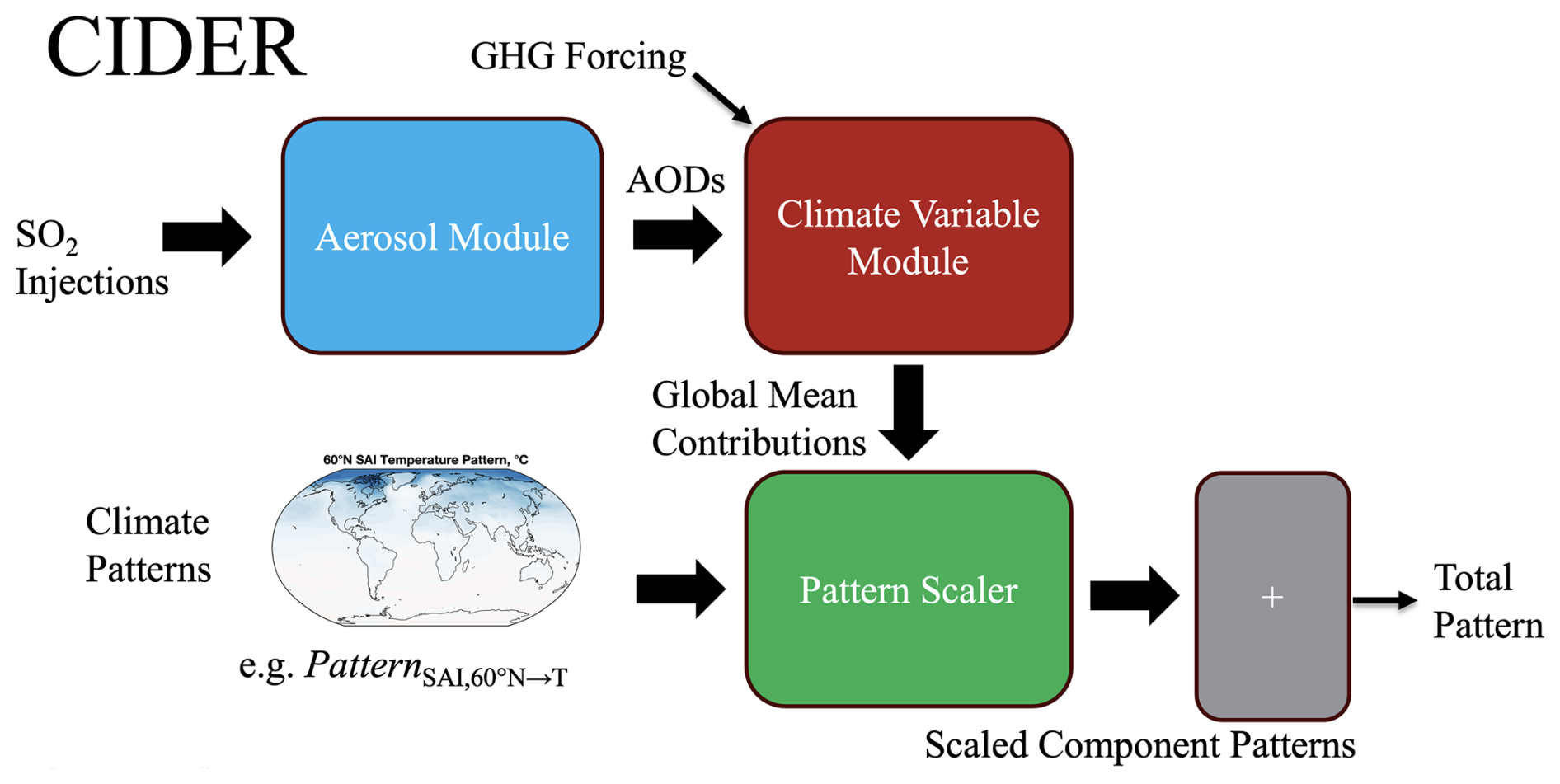
Figure 1 Diagram showing CIDER's modules. For each latitude, injection time series are input into the aerosol module, and the module generates global mean AOD time series. These are then input, along with a timeseries of GHG forcing, to model the dynamics of each climate variable (e.g., temperature or precipitation) included in CIDER. Their contributions to the global mean are calculated, and the climate variable pattern from each injection latitude is scaled by the respective contribution. These scaled patterns are then added together to provide the total global pattern in response to the aerosol injection and change in GHG concentration.

The available injection latitudes in CIDER are 60, 30, 15, 0° N, 15, 30, and 60° S. The reasoning for restricting the injection latitudes space to these locations is explained in depth in Zhang et al. (2022): briefly this is a sufficient set in CESM2-WACCM6 to capture the range of possible responses to SAI. In other words, the outcomes of any injection strategy or scenario can be also adequately expressed as some combination of injection at these latitudes.

2.3 Emulator Formulation

The dynamic responses of AOD to injection (Step 1 in Sect. 2.2) are calculated by convolving the impulse responses of AOD to injection. The impulse response is how the system behaves with respect to a sudden input signal (e.g., the ringing after one strikes a tuning fork), and convolution is adding these impulse responses in a way such that they form the system's response to a general time-varying signal. In this case, our input signals are the injection rates at each latitude, and the response of interest is that of the global mean AOD. The impulse response of the global mean AOD to injection at any particular latitude takes the form

$$\begin{array}{}\text{(1)}& g\left(t\right)=\mathit{\beta }{e}^{-(\mathit{\alpha }+\mathit{\gamma }\cdot q(t\left)\right)\cdot t}\end{array}$$

where β is a scaling capturing the equilibrium response to injection, α is the time constant, and γ is a parameter to capture the nonlinear response based on the magnitude of injection rate q(t). β and α are components of the linear response, and the sublinear response of AOD to injection rate is the most important nonlinearity to capture (via γ). All three of these parameters depend on the injection latitude. The response of AOD at some time t (in months) depends on injections at that latitude up to time t, and is thus

$$\begin{array}{}\text{(2)}& \mathrm{AOD}\left(t\right)=\sum _{j=\mathrm{1}}^{t}g\left(j\right)\cdot q(t-j)\end{array}$$

The global mean climate responses to changes in GHGs and AOD (Step 2 in Sect. 2.2) are calculated similarly, by convolving the impulse responses of the climate variable of interest to AOD or GHG forcing. The global mean response is modeled as semi-infinite diffusion, which has been used previously in climate emulators (Hansen et al., 1984; MacMynowski et al., 2011; Caldeira and Myhrvold, 2013; MacMartin et al., 2014; MacMartin and Kravitz, 2016; Farley et al., 2024). Its impulse response is of the form

$$\begin{array}{}\text{(3)}& \begin{array}{rl}& h_{x\to y}\left(t\right)=\\ & {\mathit{\mu }}_{x\to y}\left({\displaystyle \frac{\mathrm{1}}{\sqrt{\mathit{\pi }t{\mathit{\tau }}_{x\to y}^{*}}}}-e^{\left(\frac{t}{{\mathit{\tau }}_{x\to y}^{*}}\right)}\mathrm{erfc}\left(\sqrt{{\displaystyle \frac{t}{{\mathit{\tau }}_{x\to y}^{*}}}}\right)\right)\end{array}\end{array}$$

where x is a particular forcing input, y is the climate variable of interest, t is months since the emulation's start, ${\mathit{\tau }}_{x\to y}^{*}$ determines the time scale of the response, and μ_x→y is a scaling factor capturing the equilibrium climate response to the forcing input. μ_ghg→T has units °C (W m⁻²)⁻¹ and μ_ghg→P has units mm d⁻¹ (W m⁻²)⁻¹. Likewise, μ_sai→T has units °C (unit AOD)⁻¹ and μ_sai→P has units mm d⁻¹ (unit AOD)⁻¹, for all latitudes of SAI deployment. The response at time t of any climate variable to a given forcing is thus,

$$\begin{array}{}\text{(4)}& y_x\left(t\right)=\sum _{j=\mathrm{1}}^t{h}_{x\to y}\left(j\right)\cdot f_x(t-j)\end{array}$$

where f_sai,lat is the AOD above baseline for a particular latitude and f_ghg is the anthropogenic climate forcing aside from SAI (Riahi et al., 2017). At this stage, the overall global mean response can be obtained by summing the contributions y_x from each individual forcing. However, to get the projection of that global mean into a global pattern, two more steps are needed.

Step 3 proceeds with simple pattern scaling on all the individual responses:

$$\begin{array}{}\text{(5)}& Y_x\left(t\right)=y_x\left(t\right)\cdot {\mathrm{Pattern}}_{x\to y}\end{array}$$

where the two-dimensional climate variable pattern for a forcing x (denoted Y_x(t)) is defined as the product of the time-varying global mean y_x(t) (as above) and a time-invariant spatial pattern of that variable Pattern_x→y that depends on the forcing (GHGs or a specific latitude of SO₂ injection). Pattern scaling has a long history of use in climate model emulation and, for a wide variety of situations, is accurate in reproducing large-scale ESM output (e.g., Santer et al., 1990; Kravitz et al., 2017; Tebaldi et al., 2022).

Step 4 adds the 8 scaled patterns (7 latitudes of injection + GHG warming) together to produce the net change in the climate variable of interest. This relies on two different linearity assumptions, widely tested but here combined for the first time; a pattern scaling one for GHG normally used in climate emulators (from Santer et al., 1990 to Tebaldi et al., 2022), and an assumption that different patterns of cooling from SAI can be combined linearly, tested for SAI in MacMartin et al. (2017) and Brody et al. (2025). The resultant pattern is CIDER's estimation of the pattern of that climate variable at that time due to the forced responses of SAI and GHG. Evaluation of our assumptions and this pattern addition method is provided in Sect. 3.

2.4 Emulator Training

For each latitude x of SAI deployment available in CIDER, the following parameters must be trained: α_x, β_x, γ_x, which model the relationship between injection rate and global mean AOD; μ_x→y, τ_x→y, which model the global mean response of a particular climate variable y to the AOD resulting from injection at latitude x; and Pattern_x→y, which projects the pattern of the global mean response of that variable onto the globe.

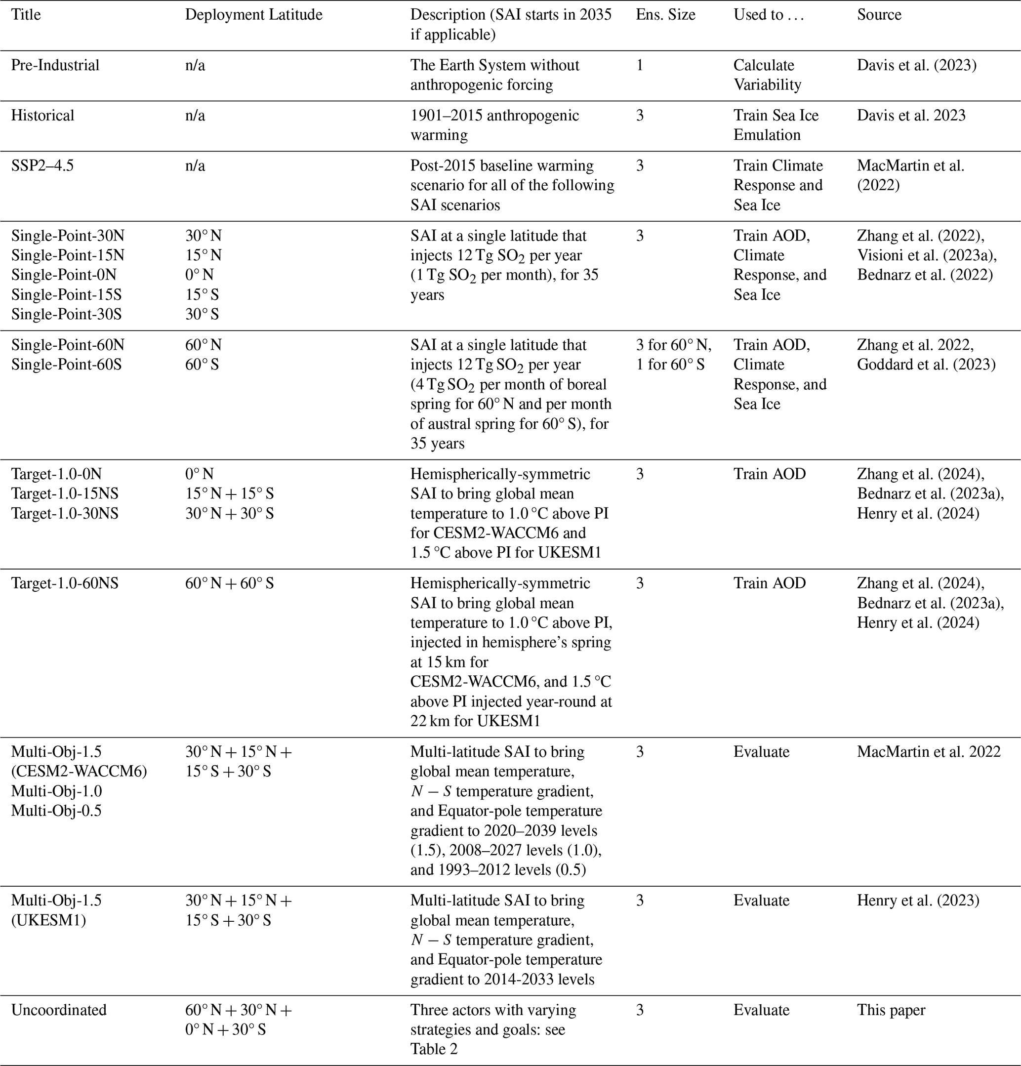
To train the three parameters that describe the global mean AOD response to injection at a particular latitude, we use two different sets of simulations (at least one ensemble member per set). Both sets are 35 years long; training on shorter lengths of simulation is fully feasible for AOD, but sets of at least this length are best to train the temperature behavior of CIDER, so we used 35 years to train the AOD too (since the data was produced regardless). The first set of simulations is the response to a step increase in injection rate at a single latitude (from 0 Tg SO₂ yr⁻¹ to a fixed 12 Tg SO₂ yr⁻¹), whose clear signal gives sufficient information to estimate α_x and β_x, the time constant and the equilibrium response. However, it gives no information about γ_x, the nonlinear dependence on injection magnitude, since it injects only at a single rate. The second simulation set we use is to train γ_x. We need a simulation with a range of injection rates at a particular latitude; for this we use strategies that maintain a constant temperature target with increasing climate change through symmetric injection about the equator. Since these simulations increase the cooling done over time, they provide a good range of injection rates for training. While training on these hemispherically-symmetric injections, we assume that the AOD resulting from simultaneously injecting at latitudes in opposite hemispheres can be added linearly; this linearity was shown in MacMartin et al. (2017). With these two sets of simulations' corresponding injection rates as input, we can find the parameters α_x, β_x, and γ_x by minimizing the root mean square error between CIDER's AOD estimation and the simulated AOD. For a full list of simulations, see Table 1.

The parameters μ_x→y and τ_x→y are found in a similar manner. We optimize a least-squares fit for each latitude of SAI in CIDER, using the 35-year global mean time series resulting from simulations with a step injection of 12 Tg SO₂ yr⁻¹. We use these simulations' global mean AOD as input and global mean values of the climate variable (emulation vs. simulation) as output. To find Pattern_x→y, the climate pattern associated with each latitude, we average the pattern of the climate variable over the last 20 years of that latitude's step response. For finding the climate response to greenhouse gas forcing, the parameters from injection to AOD are ignored and the forcing is used as in Fig. 1 – the background emissions scenario for all training simulations used is SSP2–4.5, the moderate Shared Socioeconomic Pathway that is roughly consistent with the Nationally Determined Contributions of the Paris Agreement (Burgess et al., 2020). When climate variability is needed (e.g., for Figs. 4 or 7), a long pre-industrial simulation is used to calculate and generate it (Davis et al., 2023); this assumes that the statistics of variability do not change. For a full list of simulations used, see Table 1.

Table 1 List of simulations used in this paper for both training and evaluating the emulator. Two Earth System Models are used for simulating: the Community Earth System Model version 2 with the Whole Atmosphere Community Climate Model version 6 (CESM2-WACCM6) and the U.K. Earth System Model (UKESM1). All simulations consist of a three member ensemble except for the Pre-Industrial and 60° S. n/a: not applicable

2.5 Emulation of Northern Hemisphere sea ice fraction

To emulate the response of Arctic sea ice to both greenhouse gas forcing and SAI, we developed a statistical model relating regional temperature anomalies to sea ice fraction at the grid cell level. Sea ice serves as a particularly valuable test case for our emulation approach because of its highly nonlinear response to temperature forcing - unlike many climate variables that respond approximately linearly, sea ice fraction is bounded between 0 and 1, and the its rate of change is dependent on the region's temperature. We focused on September sea ice, as this month captures the annual minimum extent in the Arctic, making it a critical indicator of long-term sea ice trends. In the Coupled Model Intercomparison Project Phase 6 (CMIP6) climate models, global annual mean temperature is a good predictor of September sea ice area, nearly independently of scenario (Notz and SIMIP Community, 2020). Here, we extend this relationship to predict the local sea ice cover as a function of local annual mean temperature.

Our analysis divides the Arctic region (60 to 90° N) into 24 distinct domains based on four longitudinal sectors and six latitudinal bands. The longitudinal sectors represent major geographic regions: I) the Pacific Ocean, II) the Atlantic Ocean, III) Eurasia, and IV) Greenland/Canada. The latitudinal bands span from 60 to 90° N in 5° increments. This regional subdivision allows us to capture spatial heterogeneity in the relationship between temperature and sea ice across different parts of the Arctic basin.

We use the CESM2-WACCM6 simulations and CIDER parameters trained to match CESM2-WACCM6. The training dataset for sea ice fraction combines three simulation sets: a historical run (1901–2015), SSP2–4.5 projections without SAI (2015–2100), and the 7 SAI single latitude injection deployment scenarios (2035–2069) (Table 1), yielding 444 total time points for each grid cell. Each set of simulations includes three ensemble members for each scenario, which were averaged to reduce the influence of internal climate variability. Temperature anomalies are calculated relative to the pre-industrial baseline period of 1850–1900.

For each of the 24 regions, we computed the spatially averaged annual mean temperature anomaly relative to pre-industrial conditions. This regional temperature anomaly as calculated by the CIDER temperature module serves as the predictor variable (x axis in Fig. 2b) and is used across all grid cells within a given region for each time step. The response variable (y axis in Fig. 2b) is the September sea ice fraction at each individual grid cell across all 259 time points.

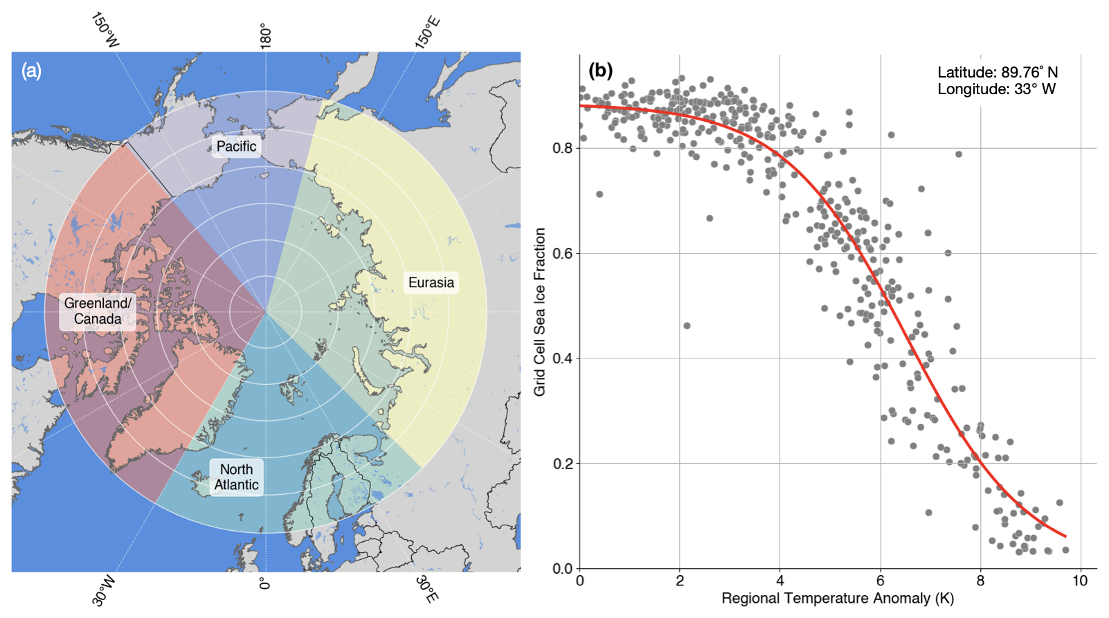
Figure 2 Regional subdivision and example logistic fit for Arctic sea ice emulation. (a) The Arctic region (60 to 90° N) is divided into 24 domains based on four longitudinal sectors (Pacific Ocean, Atlantic Ocean, Eurasia, and Greenland/Canada) and six latitudinal bands (60–65, 65–70, 70–75, 75–80, 80–85, and 85–90° N). Each region is used to calculate spatially averaged temperature anomalies that serve as the predictor variable for the logistic function. (b) Example of a logistic function fit (solid line) to annual September sea ice fraction values (points) for a single grid cell. The x axis shows the regional temperature anomaly relative to pre-industrial (1850–1900) baseline, and the y axis shows the September sea ice fraction. The logistic function captures the nonlinear transition from ice-covered to ice-free conditions as regional temperatures increase.

Given the nonlinear relationship between temperature and sea ice fraction, and the physical constraint that ice fraction must remain between 0 and 1, we fit a logistic function to the data for each grid cell. The logistic function is defined as:

$$\begin{array}{}\text{(6)}& f_i\left(T\right)=b_i+{\displaystyle \frac{L_i}{\mathrm{1}+e^{(T-T_{\mathrm{0}})k_i}}}\end{array}$$

where T is the regional temperature anomaly, f_i(x) is the predicted sea ice fraction for a grid cell i, L_i represents the amplitude of the transition from maximum to minimum ice fraction for that grid cell, T₀ is the temperature anomaly at the midpoint of the transition, k_i controls the steepness of the transition for the grid cell, and b_i is the baseline minimum ice fraction for the grid cell. We constrain k_i to be positive, so the negative sign in the exponential ensures a decreasing relationship between temperature and ice fraction (i.e., warmer temperatures lead to less ice), which is physically consistent with observed Arctic sea ice behavior. During the fitting process, L, b, and their sum are constrained to values between 0 and 1, ensuring that the predicted ice fraction remains physically meaningful and bounded within the valid range. This functional form naturally captures the transition from ice-covered to ice-free conditions as temperatures increase.

To ensure robust parameter estimation, we applied two filtering criteria during training the logistic function to exclude grid cells with insufficient data variation. First, we excluded grid cells where sea ice fraction never exceeded 0.15 across all 444 time points, as these cells remain predominantly ice-free and provide little information about the ice-temperature relationship. Second, we excluded grid cells with fewer than 10 non-zero points across the time series, as these provide insufficient information for reliable fitting. Only grid cells meeting both criteria were included in the logistic function estimations of the final emulator.

2.6 Simulation of Uncoordinated SAI

We run an example of a highly dynamic scenario of uncoordinated SAI deployment in CESM2-WACCM6, both to provide evaluation data for this emulator (and others in the future) and to analyze on its own merits. To do this, we run a three-member ensemble using the fully-coupled CESM2-WACCM6, simulating from 2035 to 2075 with the model configuration specified in Sect. 2.1 and the background emissions pathway of SSP2–4.5.

In this scenario, we have three actors deploying SAI, as detailed in Table 2; this includes (i) an actor injecting at 60°N to cool the Arctic, (ii) a second actor injecting at the equator to reduce global mean temperature, and (iii) a third actor in the Southern Hemisphere aiming to avoid disrupting tropical precipitation. This scenario is but one representative of the infinite design space of uncoordinated scenarios. In selecting this scenario, we make no claims regarding geopolitical plausibility or the likelihood of it occurring; rather, this scenario captures a number of relevant features unique to the space that may lead to interesting climate dynamics:

1. All three actors in this scenario have different climate targets – regarding both the region of interest and targeted value (defined here as the average value over a 20-year period centered on a reference year).

2. The Arctic actor begins deployment before the others, since polar SAI may be easier logistically (Smith et al., 2022; Wheeler et al., 2025).

3. The actor wanting a balanced N−S temperature gradient (for purposes of controlling the behavior of the Inter-Tropical Convergence Zone, see Kravitz et al., 2016) deploys in the hemisphere opposite to the Arctic actor but is delayed in their start.

4. The actor targeting global mean temperature terminates permanently mid-deployment (the reason is not relevant to the scenario specification). The ability for other actors to respond is limited but non-zero.

5. The remaining actors transition out of non-coordination to a coordinated, hemispherically-symmetric deployment, following the termination of Actor 2. However, this process takes time.

Since this scenario was developed in part to provide evaluation data for CIDER, injection totals were determined by using CIDER, and no feedback controller was used in the simulation, even if the targeted value would otherwise stray (e.g., if overcooling occurred in the Arctic), and the injection inputs to CESM2-WACCM6 and CIDER are identical. Additionally, the following simplifications and assumptions are applied during the uncoordinated period:

• Actors deploy using integer amounts of Tg SO₂ yr⁻¹.

• Actors can increase their injection capacity by at most 1 Tg SO₂ yr⁻¹ per year.

• As the scenario progresses, Actor 1 phases out injection as it is no longer needed to maintain its target, however it keeps half of its maximum 60° N injection capacity at the ready (8 Tg halved to 4 Tg). It can deploy it after a 1-year lag.

• It takes roughly 5 years to develop the capacity to deploy SAI in non-polar regions.

Table 2 Uncoordinated SAI actors and goals.

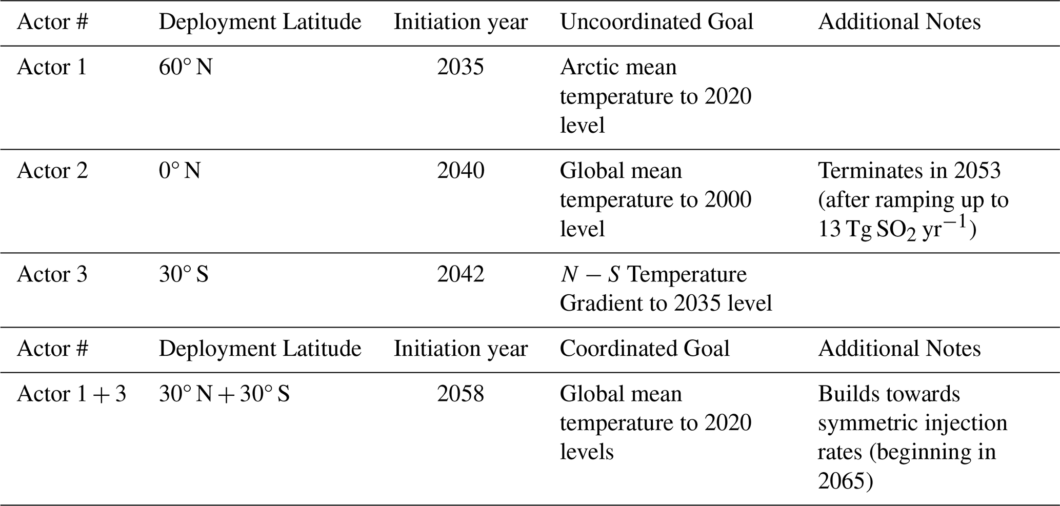
We choose for Actor 2 to undergo a termination in 2053. In response, Actor 1 redeploys half its capacity after its 1-year lag. Then, we choose for Actors 1 and 3 to begin coordinating and agree to deploy a coordinated symmetric deployment. Actor 1 begins developing capacity to inject at 30° N, to match Actor 3's 30° S; it begins developing capacity in 2053, begins deployment in 2058, and reaches symmetry with Actor 3 in 2065.

Evaluations of CIDER using this uncoordinated scenario are discussed in Sect. 3.

3 Sampling CIDER (Results)

Using the formulation in Sect. 2.3, CIDER currently is able to estimate AOD, temperature, and precipitation (as well as evaporation, with those results provided in Appendix A1). Time series that show the results of the training and testing of CIDER using CESM2-WACCM6 results are provided in Fig. 4. These time series begin in 2035 when SAI is deployed and continue for 35 years until the end of 2069. Figure 4g, h, and i show the how the emulator performs in predicting scenarios outside of the training set. These outside-of-set SAI scenarios (Multi-Obj-1.5, Multi-Obj-1.0, and Multi-Obj-0.5 in Table 1) use injection across four latitudes to fulfill three objectives simultaneously (global mean temperature, N−S temperature gradient, and equator-to-pole temperature gradient – see MacMartin et al., 2022 and Visioni et al., 2023b) for target global mean temperatures of 1.5, 1.0, or 0.5 °C above preindustrial. The emulator fits the global mean AOD, temperature, and precipitation of these multi-objective simulations for the scenario with a 1.0 °C above PI target, with a root mean square error (RMSE) of 0.01 AOD, 0.075 °C, and 0.01 mm d⁻¹ , respectively. For reference, the year-to-year standard deviation of temperature is 0.12°C and of precipitation is 0.015 mm d⁻¹ . AOD variability is harder to calculate, since much of its variability is driven by the year-to-year injection of the feedback controller, but CIDER overestimates AOD by about 5 %.

We see undercooling in the scenario with a 1.5 °C above PI target, and overcooling in the scenario with a 0.5 °C above PI target (13 % undercooling and 8 % overcooling). As the runs that were used for trained the temperature response injected 12 Tg-SO₂ per year, for roughly a degree of cooling, CIDER fits the multi-objective run that has the most similar injection rates and corresponding cooling the best; any nonlinearities in the system cause the error to grow as the amount of injection and the scenario's target stray from the values included in the training set. Similar behavior appears in precipitation, with under-reduction of precipitation for the 1.5 °C above PI case and over-reduction of precipitation for the 0.5 °C above PI case. The limitations of the linear approximation in capturing CESM2-WACCM6's nonlinearity in cooling also appeared in Farley et al. (2024), though the emulator in that paper had no pattern scaling.

Figure 3 examines the difference between the CIDER and CESM2-WACCM6 temperature and precipitation patterns for a multi-objective scenario. It also compares this with simply scaling a multi-objective scenario of a different temperature target (a simpler but less flexible approach). In Fig. 3a and b, the multi-objective for the 1.0 °C above PI scenario CIDER emulation was subtracted from the CESM2-WACCM6 simulation of the same scenario (a 3-member ensemble), and then in Fig. 3c and d the mean of those differences was normalized by the standard error at each grid cell. In Fig. 3e and f, the cooling pattern of multi-objective for the 1.5 °C above PI scenario was scaled to match the 1.0 °C above PI scenario, and then the subtraction and normalization by standard error was conducted as in Fig. 3c and d. In both temperature and precipitation, CIDER provides comparable performance to the estimation of the 1.0 °C above PI scenario as the scaling of 1.5 °C above PI.

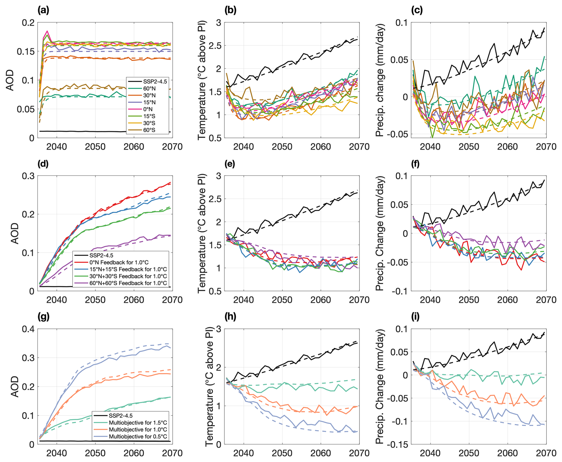
Figure 3 Time series of the CESM2-WACCM6 (solid line) global mean responses of AOD (a, d, g), near-surface air temperature above pre-industrial (b, e, h), and precipitation change from the 2020–2039 mean precipitation of SSP2–4.5 (c, f, i), along with CIDER emulations of the same (dashed line). Plots (a), (b), and (c) show the responses of the fixed injection (training data), plots (d), (e), and (f) show the responses of the symmetric injection runs for 1.0 °C above PI (also training data), and plots (g), (h), and (i) show the responses of the multi-objective runs (evaluation data).

A notable difference, however, is the large cooling spot in the Northern Atlantic Ocean. CIDER does not model Atlantic Meridional Overturning Circulation (AMOC) dynamics, and the patterns which it is scaling are those of the 12 Tg SO₂ step responses. The difference in the Northern Atlantic is likely due to the more rapid cooling of the step responses that leads to a more rapid effect on the slowing of AMOC in a way that the gradual ramp-in cooling from the multi-objective case does not (Bednarz et al., 2025). This interaction with AMOC dynamics is captured in the patterns used in CIDER, so it creates an error in this region when emulating strategies that gradually ramp-in cooling. Future versions of CIDER could include the AMOC dynamics pattern separately to correct this limitation.

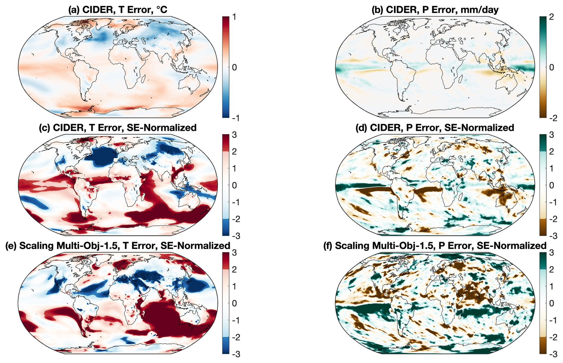
Figure 4 Error in pattern matching the multi-objective for 1.0 °C above PI scenario. A difference (CESM2-WACCM6 3-member ensemble – CIDER emulation) was taken over the last 20 years of the scenario (2049–2069) for temperature (a, c) and precipitation (b, d). For plots (c) and (d), the values in plots (a) and (b) were divided by the standard error of temperature (a) and precipitation (b) over the last 20 years at each grid cell (SE-Normalized). Grid cells less than two standard errors from the norm are whitened. For plots e and f, the pattern of cooling for the multi-objective for 1.5 °C above PI scenario was scaled by CIDER's global mean cooling and then subtracted in a similar manner to (c) and (d) to provide a comparison.

Figure 5 replicates Fig. 3, but it uses UKESM1 in place of CESM2-WACCM6. CIDER's aerosol module does slightly worse with the nonlinearity present in UKESM1's aerosol dynamics (as discussed already in Visioni et al., 2023a) – at higher injection rates, the AOD increases more slowly with increased injection rate. Additionally, the uncaptured nonlinearity to cooling in temperature and precipitation (especially the dual-polar 60° N and 60° S deployment) is more prevalent near the ends of runs in Fig. 5e and f, where there is larger injection to offset the GHG forcing. It is likely that the good emulation of the multi-objective runs’ temperature (Fig. 5h) and precipitation (Fig. 5i) is the overestimation of AOD compensating for the underestimation of the climate variable's response to forcing. While the resultant emulation achieves a correct result, it should be treated with a degree of caution (especially if one wants to extrapolate into the future, as those errors may not cancel anymore). Use of an aerosol module with zonal resolution, such as the one in Aubry et al. (2020) or Toohey et al. (2025), may aid performance in capturing the nonlinear aerosol behavior.

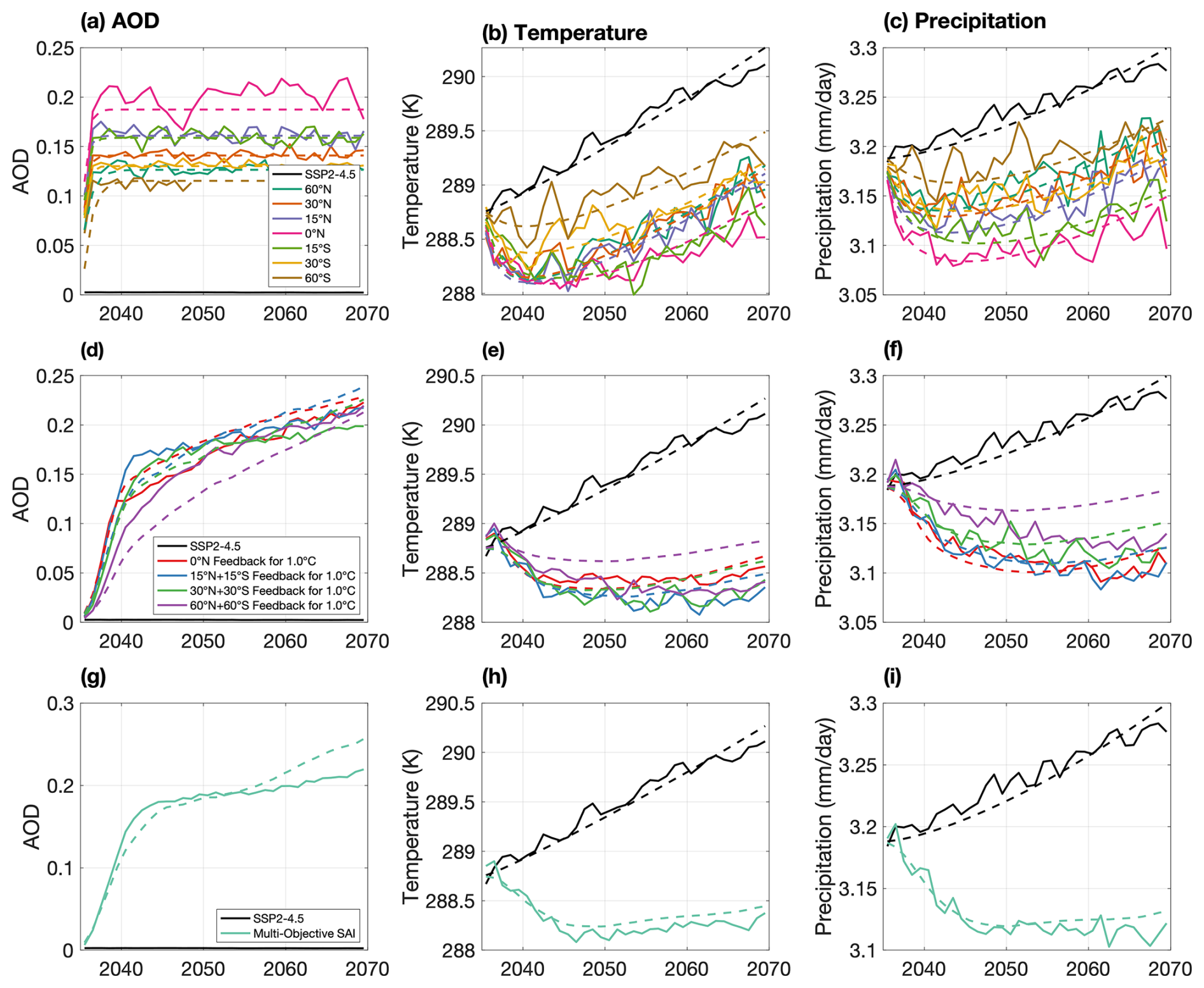
Figure 5 Time series from start of SAI deployment (2035) to simulation end (2069) of the UKESM1 (solid line) global mean responses of AOD (a, d, g), temperature (b, e, h), and precipitation (c, f, i), and CIDER emulations of the same (dashed line). Plots (a), (b), and (c) show the responses of the fixed injection, plots (d), (e), and (f) show the responses of the symmetric injection runs for 1.0 °C above PI, and plots (g), (h), and (i) show the responses of the multi-objective run.

Figure 6 displays the results of the multi-actor uncoordinated scenario described in Sect. 2.6. We compare CIDER's emulation of the scenario to the simulation in CESM2-WACCM6, using the injection rates in Fig. 6a as input to both. Overall, when comparing global mean AOD (Fig. 6b), global mean (Fig. 6c) and regional (Fig. 6d) temperature, and global mean precipitation (Fig. 6f), CIDER matches the output of CESM2-WACCM6. For Fig. 6e, although the behavior of both CIDER and CESM2-WACCM6 is similar, CIDER as currently trained seems to have an offset bias towards a warm north and cool south – this can also be seen in Fig. 4c and is likely due to the ocean dynamics that CIDER does not capture. As for the simulation itself, it is evident how each actor's behavior affects not only their progress to their own target but also others’ progress towards theirs. Even though Actor 1 and 2 are not coordinating, Actor 1 is pressured to phase out their deployment as Actor 2 phases in in order to avoid overcooling (and possibly should have phased out slightly quicker). Likewise, Actor 3's progress to their N−S temperature gradient goal is in part because they deploy in the Southern Hemisphere, but it is also in part because Actor 1 phases out their Northern Hemisphere deployment (a phase-out that Actor 1 performs in response to Actor 2). The deployments of the three actors are thus intertwined even without any explicit coordination. While in this scenario Actors 1 and 3 each put aside their individual uncoordinated goals when transitioning to the coordinated symmetric 30° N + 30° S deployment for 1.0 °C above PI, there is a non-symmetric strategy that fulfills all 3 goals (see Appendix A2).

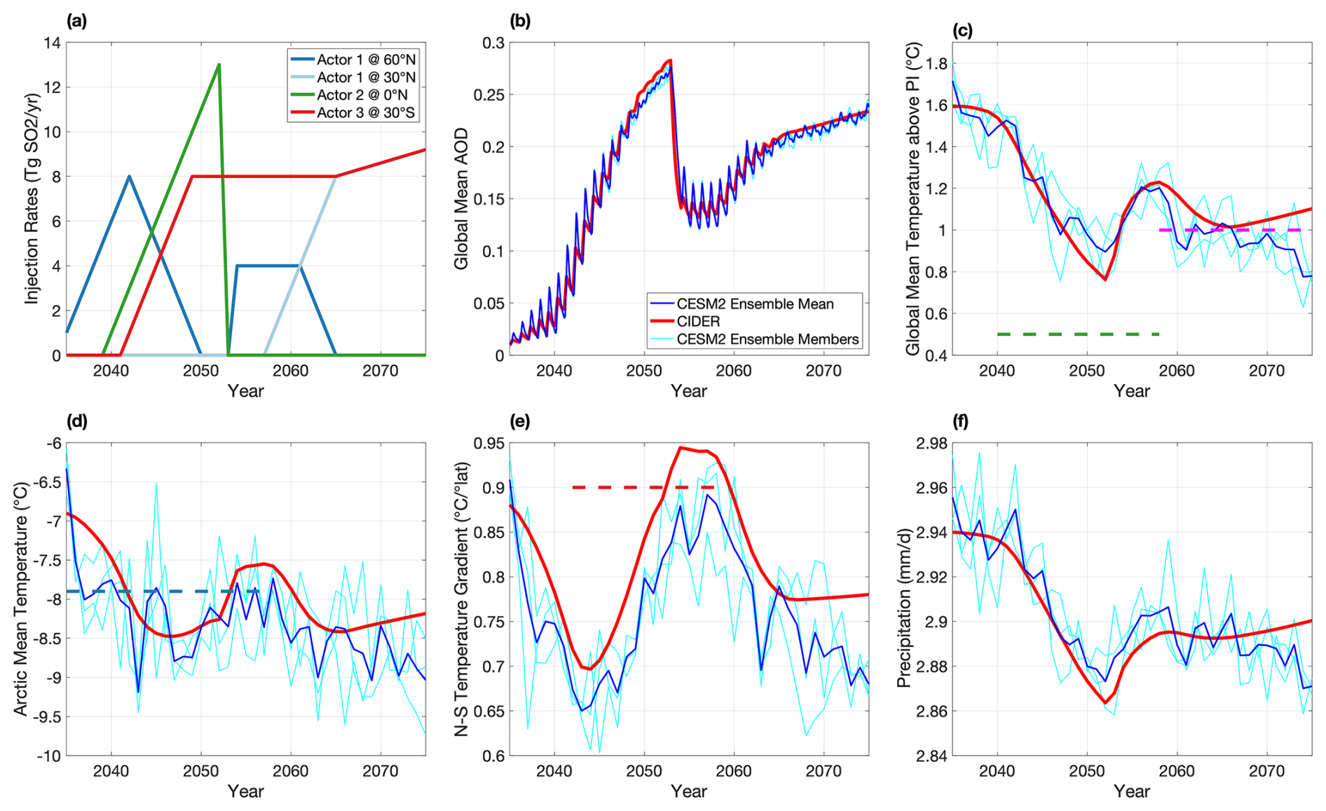
Figure 6 Time series associated with the example multi-actor uncoordinated scenario, simulated in CESM2-WACCM6 and emulated with CIDER. The time series start with SAI's deployment in 2035 and continue until the end of the simulation in 2075. (a) The annual injection rates to accomplish the goals set in Table 2. (b) Global mean AOD. A sharp drop occurs following Actor 2's termination in 2053. (c) Global mean temperature. Dashed green line indicates Actor 2's goal (which is not met prior to their termination), and dashed magenta line indicates Actor 1 + 3's coordinated goal for 2055–2075. Note the sharp but limited increase in temperatures resulting from Actor 2's termination. (d) Arctic mean temperature. The dashed blue line indicates Actor 1's goal. Note the minor overcooling that occurs because Actor 1 does not phase out quick enough during Actor 2's phase-in. (e) N−S temperature gradient (as defined in Kravitz et al., 2016). The dashed red line represents Actor 3's goal. The gradient quickly lowers as Actor 1 deploys in the Arctic, and it rises again as both Actor 3 deploys at 30° S and Actor 1 phases out to maintain 2020 Arctic temperature (rather than over-cooling). (f) Global mean precipitation. Global mean precipitation was no one's target during this simulation.

Additionally, we can combine CIDER's estimate of the forced response to SAI with simulations of climate internal variability. This combination gives emulations of SAI that include spatially and temporally coherent patterns of variability, which can be useful for analysis. Results of this combination, as well as the CESM2-WACCM6 simulations it is emulating, are shown in Fig. 7.

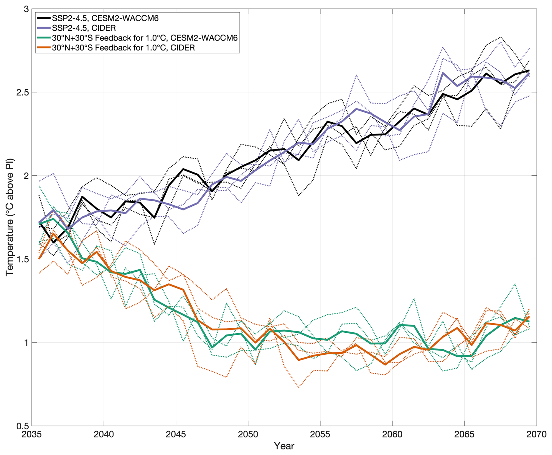
Figure 7 Adding interannual variability to the emulation time series. Variability is taken from a random subset of simulation of pre-industrial conditions, removing the mean, and then added onto CIDER's emulation. The solid lines are three-member ensemble means of the CESM2-WACCM6 simulations and CIDER emulations; the dotted lines of the same color are the corresponding individual members.

To emulate September Arctic sea ice fraction, we use CIDER's temperature output as input to the trained logistic function emulator. We assess the emulator's performance on scenarios outside the training set by emulating the September Arctic sea ice extent for the multi-objective for 1.0 °C above PI scenario and comparing a 20-year average to the 20-year average calculated from the respective CESM2-WACCM6 simulation. Figure 8a shows the CESM2-WACCM6 September Arctic sea ice extent, Fig. 8b presents the corresponding emulated results, and Fig. 8c displays the difference between simulation and emulation. The emulator generally reproduces the spatial pattern of sea ice extent well, with differences predominantly below 0.05 ice fraction across most of the Arctic basin. The hatched regions in Fig. 8c indicate where differences between the simulation and emulation are not statistically significant, while non-hatched regions show statistically significant differences. The largest discrepancies appear in transitional regions where sea ice exhibits high spatial gradients, suggesting that localized physical processes may not be fully captured by the regional temperature-based approach.

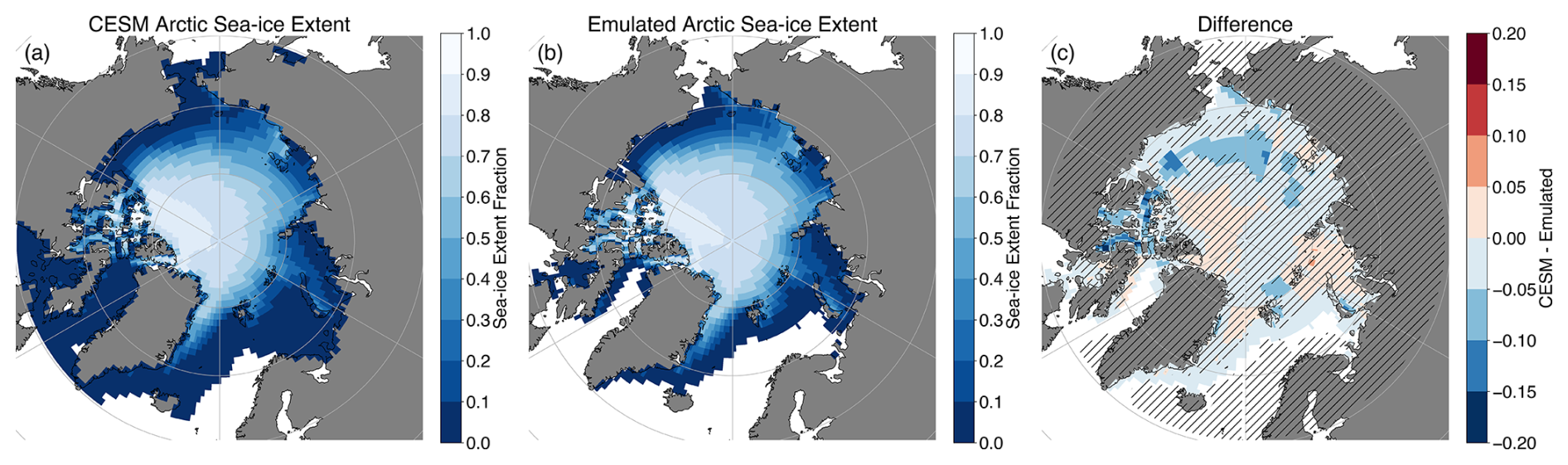
Figure 8 Comparison of September Arctic sea ice extent between CESM2-WACCM6 simulation and emulation. Twenty-year averaged (2050–2069) September Arctic sea ice fraction from (a) CESM2-WACCM6 simulation, (b) emulated results using the logistic function with CIDER temperature output as input, and (c) the difference between simulated and emulated values (CESM2-WACCM6 minus emulation). The hatched areas show statistically insignificant. The emulator reproduces the spatial pattern of sea ice extent well, with differences predominantly below 0.05 ice fraction across most grid cells. Larger discrepancies appear in transitional regions with high spatial gradients in sea ice fraction.

The logistic function fitting approach demonstrates good performance in emulating September Arctic sea ice fraction across the majority of grid cells. Figure A3 shows the distributions of error metrics and coefficient of determination (R²) values across all grid cells, while Fig. A5 displays the spatial patterns of these errors. The emulator successfully captures the large-scale patterns of sea ice evolution, with most grid cells showing good agreement between simulated and emulated values (Fig. A6).

The spatial distribution of fit quality reveals systematic patterns related to sea ice climatology. Fit quality is highest in regions where the training dataset spans a broad range of ice fractions, particularly at latitudes above 80° N where the transition from ice-covered to ice-free conditions occurs across the sampled temperature range. In these regions, the logistic function effectively captures the nonlinear relationship between temperature and ice fraction, resulting in higher R² values (typically 0.7–0.8, Fig. A4c) and lower error metrics. Conversely, regions at the higher latitudes that remain consistently ice-covered throughout most of the training period, as well as regions at lower latitudes that are predominantly ice-free, show reduced fit quality. In these regions with limited sea ice variation, the logistic function has fewer data points spanning the full range of the ice-to-no-ice transition, making it more difficult to accurately constrain the parameters that define the transition's midpoint and steepness. While the fitted function may still produce reasonable predictions within the range of observed conditions, it becomes less reliable when extrapolating beyond these conditions, given the lack of information on the transition's midpoint and steepness, leading to systematic biases. In general, regions with a high sea-ice fraction exhibit positive biases, whereas regions with a lower sea-ice fraction tend to show negative biases.

Additional validation is provided through yearly comparisons across all 24 regions for the period 2050–2069 using the multi-objective for 1.0 °C above PI scenario (Fig. A6). Figure A6 aggregates all grid cells to show the overall 1:1 correspondence between emulation and simulation. This figure demonstrates that the emulator maintains consistent performance across different regions and time periods within the validation dataset, with the aggregated results showing a tight clustering around the 1:1 line.

The observed differences between emulated and simulated sea ice likely arise from several simplifications in the emulation framework. First, by using annually averaged regional temperature anomalies rather than seasonal or monthly temperatures, the emulator does not capture intra-annual temperature variability that may influence September sea ice extent. The timing and duration of summer warming, for instance, can affect melt rates independently of the annual mean temperature. Second, the emulator does not explicitly account for sea ice dynamics, including wind-driven transport and ocean current interactions, which can redistribute ice and create local patterns not directly determined by regional temperature alone. Third, ocean heat content and subsurface warming, which play important roles in sea ice evolution, are not explicitly represented. Despite these limitations, the emulator's ability to reproduce large-scale patterns and magnitudes of sea ice extent demonstrates that regional temperature anomaly serves as a robust first-order predictor of Arctic sea ice fraction under both greenhouse gas forcing and SAI scenarios.

4 Mulling CIDER (Discussion and Conclusions)

In this paper, we described our design and evaluation of the Climate Intervention Dynamical EmulatoR, a climate emulator capable of simulating a wide array of potential future scenarios including Stratospheric Aerosol Injection. Through the input of GHG concentrations and SAI injection of sulfate precursors at different latitudes, CIDER outputs spatially and temporally resolved maps (response as a function of latitude, longitude, and time) of forced responses in surface climate variables (currently those of temperature, precipitation and evaporation) to climate change and SAI, and its projections of temperature can be extended into estimations of September Arctic Sea Ice extent. CIDER can be trained to emulate multiple climate models provided the right set of simulations is used for training (e.g., Visioni et al., 2023a; Bednarz et al., 2022). In addition, we used results from CESM2-WACCM6 and UKESM1 to demonstrate the flexibility of the framework. CIDER output can be used in analysis of a diverse set of SAI scenarios, including quickly-varying and uncoordinated deployment from multiple actors. Since CIDER is computationally inexpensive enough to be run on a laptop or website (on the order of a few seconds or less), we expect this model to be useful for various purposes, such as in real-time climate games and workshops (e.g., Rooney-Varga et al., 2020; Pereira et al., 2021), and in scenario exploration and generation, potentially in conjunction with economic models. CIDER can provide dynamically-grounded feedback on how generated scenarios would behave, and that feedback would allow participants or simulated actors to evolve their strategies in turn. This social-physical cycle may more closely resemble how climate decisions will be made in the real world, where climate models, decision-making, and impacts are interconnected. For more detailed impact analyses, CIDER cannot replace more complex climate models; however, this process can identify a subset of scenarios where it may be valuable to conduct fully-coupled climate model simulations to better evaluate outcomes.

Here, we evaluated CIDER against both “well-behaved” scenarios – scenarios which are conceived to be the work of a single actor controlling for a few (three) objectives (though these same scenarios could easily also be thought of as three actors independently controlling for one objective each, due to the structure of the control algorithm) – and against a scenario which is designed to be “poorly behaved”, including conflicting goals, staggered start times for different actors, and terminations of one but not all actors. For clarity, CIDER captures neither who deployed a particular injection of SO₂ nor why they did so – the longitude of an injection is not a part of CIDER's input, and the emulator estimates only the physical climate variables and AOD with respect to a particular set of injection rates. That said, CIDER is designed with the intent of interfacing with methods of choosing SAI injection and GHG concentration pathways that incorporate feedback to climate outcomes.

The most potentially valuable use of CIDER is in those non-standard scenarios that are very different from what has typically been simulated in SAI research to date. As we see in Fig. 3, one can achieve similar performance in estimating the multi-objective 1.0 °C above PI scenario by scaling the cooling of the 1.5 °C above PI scenario as an analog. However, a pure scaling-based approach can only be used to project outcomes from increasing or decreasing a target relative to an existing simulation, and cannot capture the behavior of any scenario involving either a different spatial distribution of injection rates, a different temporal evolution, or both. The changes of the N−S temperature gradient (as seen in Fig. 5e) as actors in the north and south phase-in and phase-out deployment is a potentially very significant feature of interest, considering that the N−S temperature gradient influences the behavior of the Intertropical Convergence Zone. Additionally, one actor's deployment of SAI (and the choices made) can influence the deployment of all the other actors, even if they are not cooperating, in highly divergent ways, since everyone is injecting into the same world. Hence, the deployment decisions still interact through the climate response. If we wanted to simulate a similar scenario but with different goals or injection locations or events, it would in general result in a very different outcome (in both injection input and climate output). Since CIDER is computationally inexpensive, it can be used in explorations of a scenario space that examine many novel and highly varying scenarios. To run this large set of scenarios with varied parameters in a climate model would likely be prohibitively computationally expensive. To run such a set of scenarios in CIDER is basically free.

By design, CIDER dynamically emulates only the forced response to GHG and SAI. In being able to estimate regionally-resolved forced precipitation and temperature (as well as any other climate variable that scales as they do), it can be used for a variety of assessments of risks. Nevertheless, it could be useful to add in additional variability to account for additional potential responses to behaviors, for example, a nation perceiving failure and thus changing their injection behavior (Keys et al., 2022). Figure 7 shows the dynamical response of CIDER with variability superimposed; the variability is taken from a random segment of pre-industrial climate simulation. These runs with variability can even form their own ensemble, for direct comparison with simulation ensembles of the same ensemble size. In principle, our method of adding variability is just one approach. CIDER could in the future be coupled with an emulator of internal variability (e.g., Link et al., 2019; Nath et al., 2022; Bassetti et al., 2024) to generate the combination of forced and unforced response while keeping file size low.

As any tool, we can imagine many future improvements for CIDER. At its current stage, CIDER outputs AOD, temperature, precipitation, and evaporation fields, and it can extend its temperature output to sea ice extent. The sea ice extent emulation demonstrates how variables with well-defined physical relationships to local temperature can be incorporated through targeted statistical modeling, even when those relationships are nonlinear. The logistic function approach achieves strong performance in relating regional temperature anomalies to grid-cell-level September sea ice fraction, though it inherits some limitations from relying solely on temperature, such as not explicitly capturing sea ice dynamics or intra-annual temperature variations. This approach could serve as a template for incorporating other nonlinearly-related climate variables into CIDER. Future iterations can include more variables of interest that have a functional relationship with global or regional temperatures (e.g., deposition of sulfate related to injection rates, heat extremes, precipitation extremes, day/night average temperature), and training to estimate these would be as simple as following the process used for training temperature, precipitation, evaporation and sea-ice in Sect. 2.4 or 2.5 with the new variable.

Future iterations can include more variables of interest that linearly scale reasonably well with the above (e.g., deposition of sulfate, heat extremes, precipitation extremes, day/night average temperature), and training to estimate these would be as simple as following the process used for training temperature, precipitation, and evaporation in Sect. 2.4 with the new variable. Also, even though CIDER currently provides monthly-resolved climate output, it lacks a seasonal cycle. In theory, CIDER's climate module could be expanded to include unique dynamics for each month or season. Implementing this seasonal dynamical change would likely include dividing the emulator to go across whatever temporal resolution was desired (e.g., in 12 for capturing the per-month dynamics), training parameters for each slice (e.g., parameters for Januarys, Februarys, Marches), and then recombining them at the end. Since assessment of climate impacts often requires information about how the climate extremes or timing of certain events within a given year have changed, these two improvements to CIDER would be sensible next steps, with the training to estimate extremes being the easier of the two. Additionally, as Fig. 4 shows, the current form of CIDER does not capture AMOC dynamics. An additional set of dynamics could be integrated into CIDER to better estimate the ocean response to different strategies of SAI. Other forms of climate intervention (e.g., marine cloud brightening or space mirrors) could also be integrated into CIDER, but any significant nonlinear effects they have on the climate must be accounted for in their implementation, since CIDER's pattern scaling will not capture them as currently implemented.

For fitting its parameters, CIDER currently uses optimization to reduce RMSE relative to its training data set, but future steps may include taking a Bayesian approach to parameter tuning (e.g., Dorheim et al., 2020 or Bouabid et al., 2024). However, the natural variability present in the training data is not the only source of uncertainty. CIDER has several sources of uncertainty, namely in the parameters it fits, its parametric form, and the model it fits. CIDER's simplified form (described in Sect. 2.2) does not account for all dynamics in CESM2-WACCM6 and UKESM1, and thus differences will appear even in the best-fit parameters. There is potential for the model parametric form to both not account for all the dynamics involved and not account for all sources of nonlinearity. Both of these lead to some residual differences relative to the training and testing data even with the best fit parameters. Furthermore, changing the relative weighting on the different simulations in the training data set will result in different best-fit parameters. The emulator in Farley et al. (2024) uses a modified version of EVA-H (Aubry et al., 2020) as its aerosol module, and it is able to capture the AOD responses of 0.5, 1.0, and 1.5 above PI very well. Farley et al. (2024)'s emulator uses the same climate variable dynamics module as the one in this paper, and it has the same issue with nonlinearity to different amounts of forcing that one can see in Fig. 3 but especially Fig. 5. Substituting in other dynamic models for the aerosol, climate variable, pattern scaling, and pattern-combining modules could yield better results. Doing so could also allow one to glean more dynamical information from the same emulator run (e.g., stratospheric residence time of the aerosols as in Toohey et al., 2025) or capture AMOC dynamics. Lastly, CIDER trains to fit the training data, which comes from a particular climate model or models, in our case CESM2-WACCM6 and UKESM1. By definition, climate features which these models do not capture well, CIDER will not capture well either. Future steps to address this could include training and testing CIDER onto a wider ensemble of different models and for all of their emulated outputs to be available in response to the same input, integrating a robust representation of inter-model uncertainties that could be provided together with the mean response values.

As a final note, it is possible to substitute in a machine learning model for any of CIDER's dynamic modules, but some caution is warranted. For instance, if one only saw Fig. 5h or i, one could conclude that UKESM1's multi-objective simulations are well-estimated and then place too much confidence in this reduced order model. Machine learning's tendency to overfit data while often not allowing to explain the results only makes this phenomenon worse. It is only because we can break CIDER into its component parts, run diagnostics, and explain each parameter within that we can draw accurate conclusions on CIDER's performance and find areas for improvement.

Appendix A

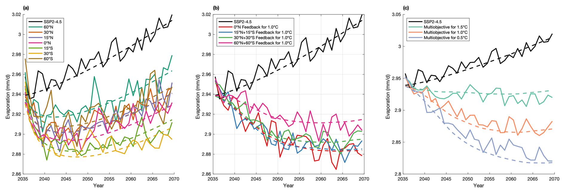
Figure A1 CESM2-WACCM6 (solid line) global mean responses of evaporation along with CIDER emulations of the same (dashed line). (a) shows the responses of the fixed injection (training data), (b) shows the responses of the symmetric injection runs for 1.0 °C above PI (also training data), and (c) shows the responses of the multi-objective runs (test data).

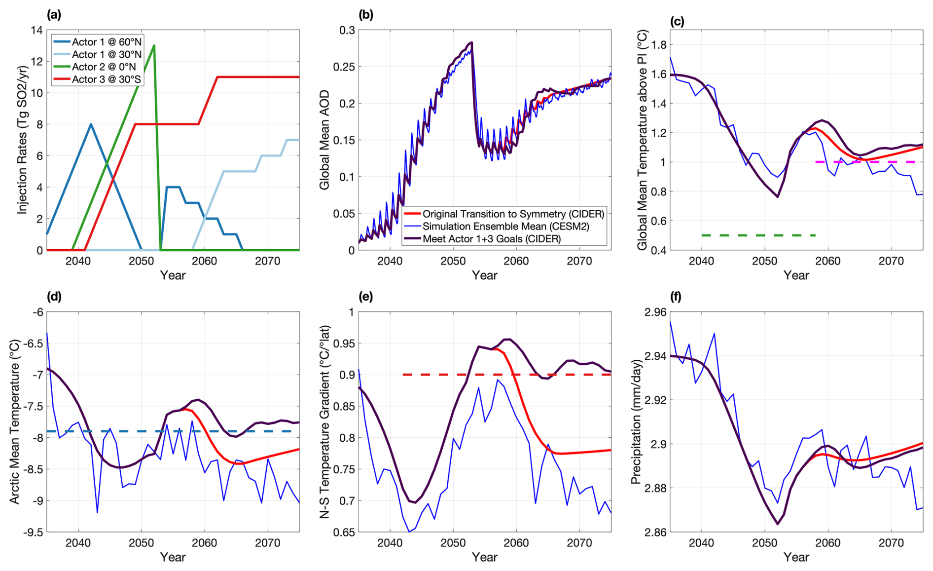
Figure A2 Example multi-actor uncoordinated scenario in CESM2-WACCM6 and emulated with CIDER from Sect. 2.6, along with a non-symmetric strategy that fulfills the individual goals of Actor 1 and 3.

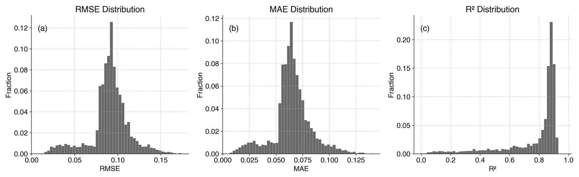
Figure A3 Distribution of fit quality metrics for Arctic sea ice emulation. Histograms showing the distribution of (a) root mean square error (RMSE), (b) mean absolute error (MAE), and (c) coefficient of determination (R²) across all 5302 valid grid cells. The logistic function achieves RMSE below 0.1 for 71.7 % of grid cells and R² above 0.8 for 68.7 % of grid cells, demonstrating strong overall performance in capturing the temperature-sea ice fraction relationship.

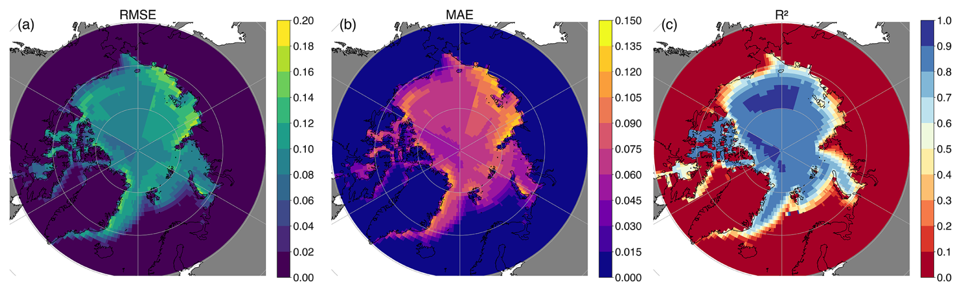
Figure A4 Spatial distribution of fit quality metrics for Arctic sea ice emulation. Maps showing (a) root mean square error (RMSE), (b) mean absolute error (MAE), and (c) coefficient of determination (R²) for each grid cell.

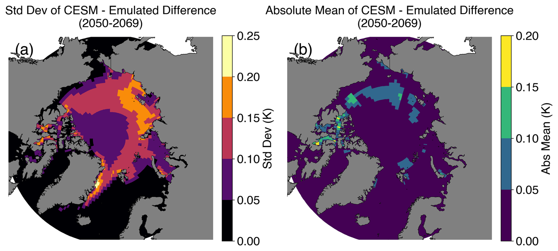
Figure A5 Spatial distribution of the error for Arctic sea ice emulation. Maps showing (a) the standard deviation of CESM – Emulated sea ice fraction for 20 years (2050–2069), and (b) the absolute mean of CESM – Emulated sea ice fraction for 20 years (2050–2069).

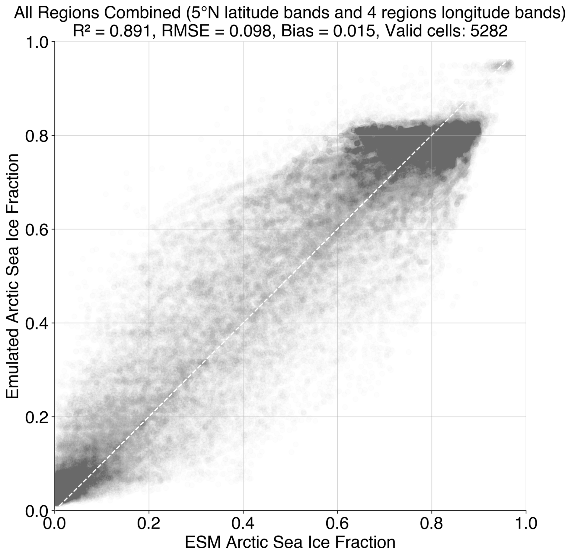
Figure A6 Aggregated performance of sea ice emulation across all regions. Scatter plot comparing emulated September Arctic sea ice fraction (y axis) to CESM2-WACCM6 simulated values (x axis) for all grid cells and all 24 regions combined. Twenty years of annual values from 2050–2069 are shown. The dashed line represents the 1:1 relationship.