Conditional diffusion models for downscaling and bias correction of Earth system model precipitation

Climate change exacerbates extreme weather events like heavy rainfall and flooding. As these events cause severe socioeconomic damage, accurate high-resolution simulation of precipitation is imperative. However, existing Earth System Models (ESMs) struggle to resolve small-scale dynamics and suffer from biases. Traditional statistical bias correction and downscaling methods fall short in improving spatial structure, while recent deep learning methods lack controllability and suffer from unstable training. Here, we propose a machine learning framework for simultaneous bias correction and downscaling. We first map observational and ESM data to a shared embedding space, where both are unbiased towards each other, and then train a conditional diffusion model to reverse the mapping. Only observational data is used for the training, so that the diffusion model can be employed to correct and downscale any ESM field without need for retraining. Our approach ensures statistical fidelity and preserves spatial patterns larger than a chosen spatial correction scale. We demonstrate that our approach outperforms existing statistical and deep learning methods especially regarding extreme events.

1 Introduction

With global warming, we anticipate more intense rainfall events and associated natural hazards, e.g., in terms of floods and landslides, in many regions of the world (IPCC, 2023). Understanding and accurately simulating precipitation is particularly important for adaptation planning and, hence, for mitigating damages and reducing risks associated with climate change. Earth System Models (ESMs) play a crucial role in simulating precipitation patterns for both historical and future scenarios. However, these simulations are computationally extremely demanding, primarily because they require solving complex partial differential equations. To manage the computational load, ESMs resort to approximate solutions on discretized grids with coarse spatial resolution (typically around 100 km). The consequence is that these models do not resolve small-scale dynamics, such as many of the processes relevant to precipitation generation. This leads to considerable biases in the ESM fields compared to observations. Moreover, the coarse spatial resolution prevents accurate projections of localized precipitation extremes. Therefore, precipitation fields simulated by ESMs cannot be used directly for impact assessments (Zelinka et al., 2020) and especially tasks such as water resource and flood management, which require precise spatial data at high resolution (Gutmann et al., 2014).

Statistical bias correction methods can be used as a post-processing to adjust statistical biases. Quantile mapping (QM) is the most common method for improving the statistics of ESM precipitation fields (Tong et al., 2021; Gudmundsson et al., 2012; Cannon et al., 2015; Miao et al., 2019). QM reduces the bias using a mapping that, locally at each grid cell, aligns the estimated cumulative distribution of the model output with the observed precipitation patterns over a reference time period. Although QM is effective in correcting distributions of single grid cells, it falls short in improving the spatial structure and patterns of precipitation simulations (Hess et al., 2022). A visual inspection shows that ESM precipitation remains too smooth compared to the observational data after applying quantile mapping.

To address these problems, deep learning methods have recently been introduced (Pan et al., 2019; Li et al., 2022; Hess et al., 2023; Pan et al., 2021; François et al., 2021; Hess et al., 2022). In these approaches, the statistical relationships between model simulations and observational data are learned implicitly. A general constraint when using machine learning methods for bias correction is that individual samples of observational and Earth System Model data are always unpaired. In this context, a sample is a specific weather situation at a specific point in time. The reason for this lack of pairs is that simulations, even with very similar initial conditions, diverge already after a short period of time due to the chaotic nature of the underlying atmospheric dynamics. Currently, one can, therefore, not utilize the wide range of supervised machine learning (ML) techniques that have shown great success in various disciplines in recent years and the available options are consequently restricted to self- and unsupervised machine learning methods. Recent studies (Hess et al., 2023; Pan et al., 2021; François et al., 2021; Hess et al., 2022) applied generative adversarial networks (GANs) (Goodfellow et al., 2020) and specifically cycleGANs (Zhu et al., 2017) to improve upon existing bias correction techniques. A major limitation of GAN-based approaches is that the stability and convergence of the training process are difficult to control and that it is challenging to find metrics that indicate training convergence. In addition, GANs often suffer from mode collapse, where only a part of the target probability distribution is approximated by the GAN.

As noted above, the low spatial resolution of ESM fields prevents local risk and impact assessment, necessitating the additional use of downscaling methods. In line with the climate literature, we refer to increasing the spatial resolution as downscaling throughout our manuscript, although we are aware that, especially in the machine learning literature, the term upsampling is more prevalent. We use the term downscaling only when we want to increase the information content in an image as well as the number of pixels. When we refer to upsampling (downsampling), we only mean an increase (decrease) in the number of pixels. Statistical downscaling aims to learn a transformation from the low-resolution ESM fields to high-resolution observations. Recent developments lean towards using machine learning methods for this task (Rampal et al., 2022; Hobeichi et al., 2023; Rampal et al., 2024). The potential for machine learning-based downscaling methods was already shown in (Vandal et al., 2017; van der Meer et al., 2023; Doury et al., 2023, 2024; Rampal et al., 2025).

Recently, Hess et al. (2025) used an unconditional consistency model (CM) for downscaling 3°×3.75° precipitation data to 0.75°×0.9375°. Our work addresses the more challenging task of downscaling from 1°×1.25° to 0.25°×0.25° resolution, a scale essential for regional impact assessments. We show that the consistency model applied to our higher resolution setting with limited amounts of training data struggles to approximate the distribution, highlighting an advantage of our conditional training approach. The analysis is further extended to out-of-distribution scenarios, particularly those involving extreme precipitation and future emission projections.

Diffusion models (DMs) have recently emerged as the state-of-the-art ML approach for conditional image generation (Saharia et al., 2022b; Rombach et al., 2022; Saharia et al., 2022c) and image-to-image translation (Saharia et al., 2022a), mostly outperforming GANs across different tasks. Diffusion models (Figs. 1 and S1 in the Supplement) avoid the common issues present with GANs in exchange for slower inference speed. A diffusion model consists of a forward and a backward process. During the forward process, noise is added to an image in subsequent steps to gradually remove its content. The amount of noise added follows a predefined equation. During the backward process, a neural network is trained to reverse each of these individual noising steps to recover the original image. The trained diffusion model can generate an image of the training data distribution, given a noise image as input. Recent work (Wan et al., 2024) introduced a framework for downscaling and bias correction, combining a diffusion model that is responsible for downscaling and a model based on optimal transport responsible for bias correction. Optimal transport (Cuturi, 2013) learns a map between two data distributions in an unsupervised setting. However, this framework is computationally expensive and has so far only been demonstrated on synthetic datasets, without evaluation on real-world observational or ESM fields. In contrast, our approach is computationally efficient by combining computationally efficient QM for large-scale bias correction with a conditional diffusion model that performs both small-scale bias correction and downscaling by generating matching small-scale patterns. We demonstrate its effectiveness for precipitation data, highlighting its ability to correct biases, downscale accurately, and capture extremes, uncertainties, and trends. A major advantage is that our conditional training allows us to use a relatively small dataset for training and still capture the distribution accurately. In contrast, unconditional models often need considerably more data to capture the full data variability, as we also show in our comparison to Hess et al. (2025) (see Fig. S2).

Figure 1 Schematic overview of our approach. (a) Bias correction and downscaling can be formulated as a mapping ω from the ESM data space to the data space of observations (OBS) used for training. We first map both datasets to a shared embedding space and then learn the inverse of the mapping f with a DM. We achieve a correction of the ESM data by applying DM∘g. (b) Our framework allows to train a single model for bias correction and downscaling in a supervised way despite the unpaired nature of OBS and ESM fields. We construct functions f, g that map OBS∈V^obs and ESM∈V^esm fields to a shared embedding space V^emb. Note that this embedding space does not enforce pairing between individual fields, but a similar distribution between the embedded fields. By inverting f, we can rewrite ω as $\mathit{\omega }=f^{-\mathrm{1}}\circ g$. We learn the inverse f⁻¹ with a conditional diffusion model. This model is trained (blue arrow) on pairs of observational data to approximate the map from f(OBS) to OBS. Because f(OBS) and g(ESM) share the embedding space (and are identically distributed by construction), we can evaluate (green arrow) the DM on the embedded ESM data g(ESM) and thereby approximate the bias correction and downscaling function $\mathit{\omega }=f^{-\mathrm{1}}\circ g\approx \mathrm{DM}\circ g$, without the need of paired data between OBS and ESM. (c) Left panels: training process of the conditional DM $\mathrm{DM}\approx f^{-\mathrm{1}}$. Note that the individual samples of the input OBS and their embeddings f(OBS), as well as the embeddings f(OBS) and the output of $\mathrm{DM}\approx f^{-\mathrm{1}}$ are paired, respectively. Right: Inference process of $\mathrm{DM}\approx f^{-\mathrm{1}}$. In this case, the individual samples of the input ESM, their embeddings g(ESM), and the output of $\mathrm{DM}\approx f^{-\mathrm{1}}$ are paired, respectively. It is not necessary for the training embedding samples to be paired with the inference embedding samples.

Existing work leveraging state-of-the-art ML methods for bias correction and downscaling does not systematically investigate out-of-distribution scenarios like future emission scenarios and especially the representation of extreme events of the generative models in detail. Understanding the generalization performance of the models under these conditions is, however, crucial for impact modelers who rely on these outputs for risk assessments under future climate conditions. We will therefore present a detailed analysis of the generalization capability of our approach, both in terms of its performance in preserving climate change trends, as well as in capturing extreme events and their trends.

A major challenge in bias correction and downscaling of ESMs is that the whole class of state-of-the-art supervised machine learning methods is not applicable in this setting. This is due to two fundamental issues. First, due to the chaotic nature of atmosphere and ocean dynamics, ESM simulations and observational data are inherently unpaired. This means that the weather on a specific day in an ESM simulation does not correspond to the observed weather on the same day, which prevents directly training a supervised ML method on the task. Second, training a ML model on observational data and applying it to ESM data is unreliable due to the substantial distribution shift between both datasets caused by systematic biases in the ESM. This violation of the assumption of independently and identically distributed (i.i.d.) data leads to poor generalization. Our proposed framework directly addresses both challenges. We reformulate the problem in a novel way, which allows us to train arbitrary ML models in a conditional setup without the need for explicit ESM-observation pairs, while at the same time resolving the distribution shift.

We present a novel framework based on state-of-the-art conditional diffusion models that allows us to perform both bias correction and downscaling with one single neural network, which only takes precipitation as input and output. We use a conditional diffusion model (Figs. 1 and S1) to correct low-resolution (LR) ESM fields toward high-resolution (HR) observational data (OBS). The supervised formulation of the task allows us to train a conditional diffusion model that is more data efficient (requiring less training data) than its unconditional counterpart because it is trained to only learn the small-scale precipitation patterns, given the large-scale patterns. The model then learns to copy the correct large-scale information from the condition channel. An unconditional model that learns to approximate the full distribution of precipitation at all scales is unnecessarily complex for the task. In general, our task of bias correction and downscaling can be seen as taking a field from a distribution p(ESM) and transforming it into a field from a conditional distribution p(OBS|ESM).

A key idea of our framework is to reformulate the problem in a way that yields a clear training objective. A key part of it is a statistical mapping to an embedding space, which ensures that training and inference data are identically distributed. We achieve this by introducing transformations f and g that map observational (OBS) and ESM data to a shared embedding space (see Methods and Fig. 1a). This space is explicitly designed to solve the two fundamental issues mentioned above: it creates a valid supervised objective by providing paired samples of observational data and their perturbed embeddings (OBS, f(OBS)), and it ensures the training and inference distributions match by making the distributions of the embeddings f(OBS) and g(ESM) similar. On this shared embedding space, we can train a conditional diffusion model to approximate the inverse of f (Fig. 1b and c). The neural network is trained to predict the clean OBS data given the embedded OBS data, thereby only relying on pairs between OBS and f(OBS). For inference, the ESM data is mapped into the same embedding space using the transformation g. The statistical similarity of the resulting embeddings f(OBS) and g(ESM) enables the diffusion model, which was trained exclusively on observational data, to generalize effectively to downscale and bias-correct the ESM fields. The diffusion model will map the embedded ESM data towards the distribution of observational data, resulting in bias-corrected and downscaled ESM fields.

This framework offers great flexibility as it can be applied to any ESM, with minimal adjustments in the embedding pipeline. The embedding transformation for the ESM has two key components. First, we use quantile mapping (QM) as a fast and effective method to correct large-scale biases in the ESM. Second, we introduce noise to remove small-scale information in the precipitation fields. We define large scales as those spatial scales that are effectively corrected using QM alone, while smaller spatial scales, which require additional correction, are referred to as small scales (Fig. 2). This noise selectively targets small-scale patterns, leaving intact large-scale patterns. In our approach, quantile mapping addresses large-scale biases, while the small-scale biases and downscaling are handled by our diffusion model. The task of our model is then to perform downscaling and bias correction by regenerating these small-scale features, in a way that ensures consistency with the preserved large-scale patterns. When applying our framework on a different region or ESM, it is computationally inexpensive to recompute the quantile mapping (QM) for the embedding transformation.

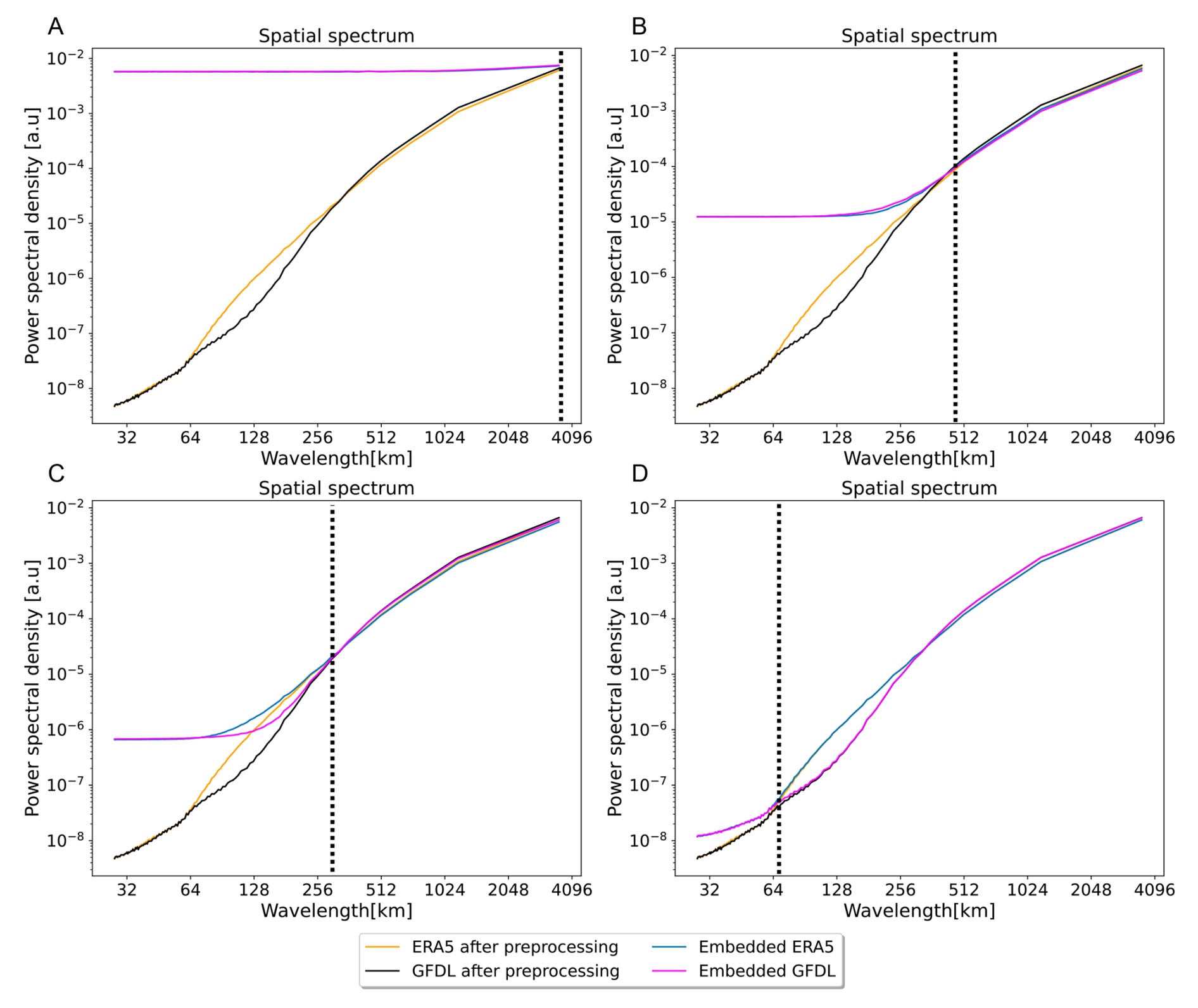
Figure 2 Power spectral densities (PSDs) for different choices noising scale of the diffusion model. The noising scale s (dashed line) is a hyperparameter that can be chosen depending on the ESM and observational datasets, as well as on the specific task. For the maximal choice of s (a) all information in the observations (ERA5) and model simulations (GFDL) is noised and thereby destroyed. Conditioning on pure noise makes the task equivalent to unconditional image generation. The diffusion model will learn to generate observational fields with no relation to the ESM fields. When s is chosen to be minimal, there will be no noising and the conditional generation will directly replicate the condition, i.e. the ESM field. In (b) we chose s as the point where the PSDs of the observational and simulated datasets intersect. We then apply sufficiently many forward diffusion noising steps to both datasets, destroying small-scale structure until they agree in the PSD. We call scales smaller than s small scales and scales larger than s large scales. In (c) and (d), the effects of choosing a smaller noise scale s are shown. Prior knowledge about the ESM or its accuracy can also guide the choice of s.

2 Results

The ability of the diffusion model DM to approximate f⁻¹ and the effectiveness of the transformations f, g will determine the overall performance of the downscaling and bias correction model $\mathit{\omega }=\mathrm{DM}\circ g$. Therefore, we first investigate the effectiveness of the embedding transformation f and g, followed by an analysis of the downscaling and bias correction performance of the diffusion model DM, on the observational dataset. Once we have shown that both work as expected, we investigate the performance of the diffusion model in bias correction and downscaling of the ESM precipitation fields. Without loss of generality, we chose the 0.25° ERA5 reanalysis (Hersbach et al., 2020) data as observational data and the state-of-the-art GFDL-ESM4 (Dunne et al., 2020) at 1° as our ESM.

2.1 Embedding evaluation

Transformations f, g are chosen so that they map observational (OBS) and model (ESM) data to a common embedding space V^emb, where all samples are identically distributed. For constructing f and g we need f(ERA5) and g(GFDL) to be unbiased with respect to each other. The transformations need to be chosen such that the embedded data share the same distribution and the same power spectral density (PSD). We assess if they are statistically unbiased towards each other by analyzing their histograms and latitude / longitude profiles, as well as their spatial PSDs (after applying pre-processing transformations). Figure S3 shows that f(ERA5) and g(GFDL) have the same spatial distribution (Fig. S3a) with minor differences in temporal statistics shown by the histogram (Fig. S3b) and latitudinal/ longitudinal profiles (Fig. S3c and d).

The individual operations that make up the transformations f and g do not change the large-scale patterns of their respective inputs, as desired for a valid bias correction. The goal of downscaling and bias correction ω (Fig. 1) is to rely on the unbiased large-scale patterns of the ESM and correct statistics, as well as small-scale patterns. The transformation g preserves the unbiased information from the ESM by construction. Therefore, we want the diffusion model, approximating f⁻¹, to also preserve unbiased information.

The extreme case of erasing all detail with large amounts of noise (Fig. 2a) leads to learning the unconditional distribution p(ERA5), which is then not a correction of GFDL but a generative emulation of the ERA5 reanalysis data. We tested this by adding the same amount of noise to the output of our diffusion model that was added to create g(GFDL). This ensures that both the downscaled and bias-corrected fields, as well as the original GFDL fields, lack the small-scale details up to the same point.

To verify that large-scale patterns are preserved by the diffusion model, we compute image similarity metrics between the low pass filtered version of the input of the diffusion model (embedded ERA5 data f(ERA5)) and the low pass filtered output of the diffusion model DM(f(ERA5)). The output of the low pass filter leaves the large-scale features unchanged. The comparison yields an average structural similarity index (SSIM) (Wang et al., 2004) value of 0.85 and a Pearson correlation coefficient of 0.95 for the validation dataset. This verifies that large-scale patterns are well preserved by the diffusion model.

Our diffusion model is able to reconstruct high-resolution fields following the ERA5 distribution from embedded ERA5 fields f(ERA5), with only minor discrepancies in small-scale patterns (Fig. S4a). A comparison between the mean absolute spatial-temporal difference between the first downsampled and then bilinearly upsampled ERA5 and the ground truth ERA5 fields at 0.25° yields a mean bias of 0.27 mm d⁻¹. The downscaling of our diffusion model reduces this bias to 0.21 mm d⁻¹ (at 0.25°). Our diffusion model thus approximates f⁻¹ well, and we successfully created a shared embedding space in which f(ERA5) and g(GFDL) are identically distributed.

2.2 Evaluation of downscaling and bias correction performance

We investigate the inference performance of our diffusion model on embedded GFDL data g(GFDL). We compare the downscaling and bias correction performance of our diffusion model to a benchmark consisting of first applying bilinear upsampling followed by QM for bias correction.

Figure 3 presents a qualitative comparison between the different individual precipitation fields. The upsampled GFDL fields, as well as our benchmark are visually too smooth. They therefore appear blurry compared to the ERA5 precipitation fields despite having the same spatial resolution of 0.25°. Our diffusion model produces high-resolution detailed outputs that are visually indistinguishable from the ERA5 reanalysis that we treat as the ground truth. We also compared our diffusion model to a different state-of-the-art diffusion model implementation, EDM (Karras et al., 2022). The EDM model was trained for the same number of epochs, while taking twice as long for one. The EDM almost perfectly corrects the spectrum (Fig. S5a). However in both the histogram (Fig. S5b) as well as in latitudinal and longitudinal profiles (Fig. S5c and d) the EDM model is inferior to our proposed diffusion model. We also compared our method against a VQ-VAE-based generative model, finding that our model outperforms it across these metrics (for details, see Sect. S3 and Fig. S6).

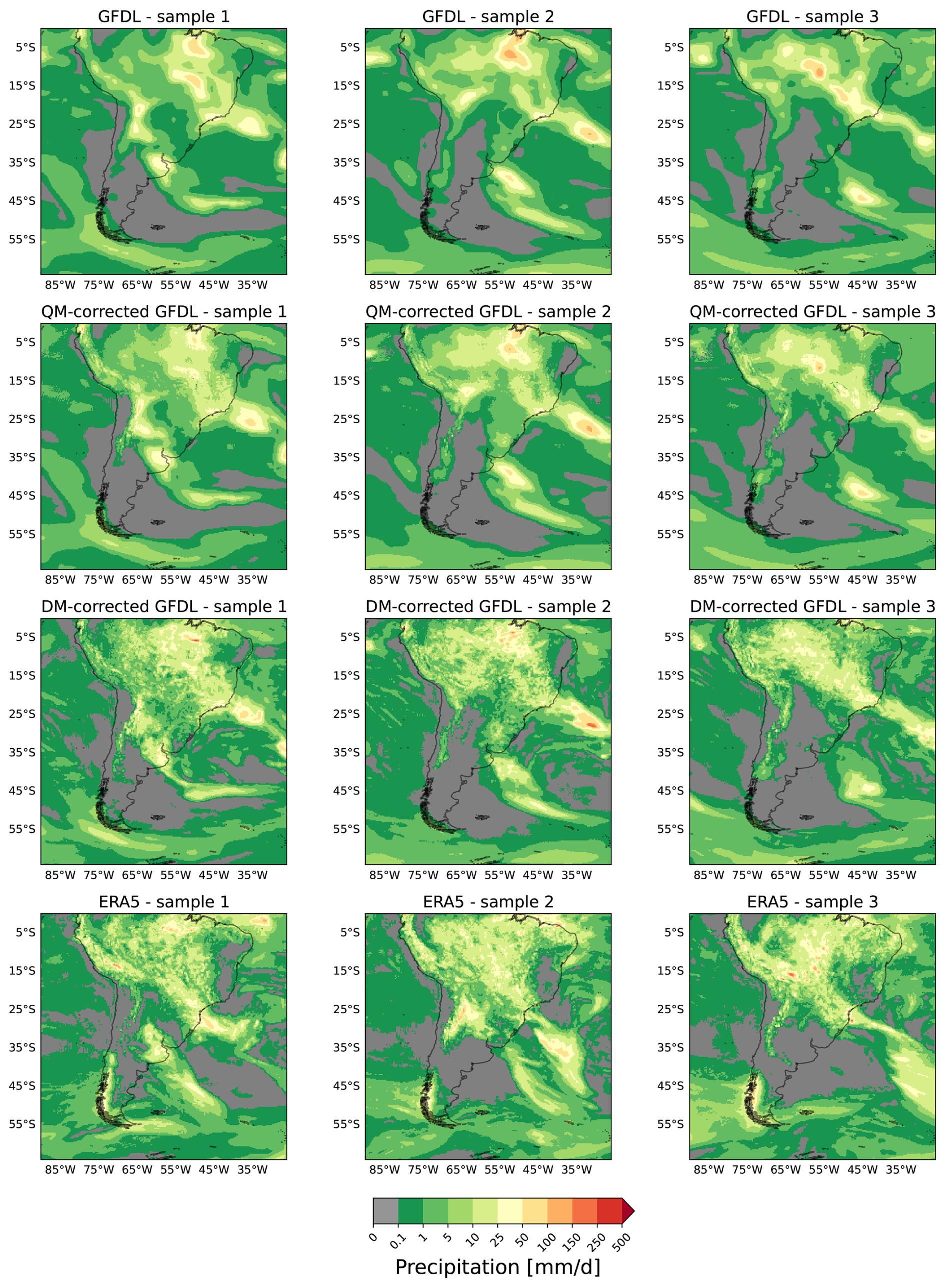
Figure 3 Comparative visualization of individual randomly selected samples. Each row presents three samples of the same dataset. The top row shows GFDL ESM4 data, bilinearly upsampled to 0.25° to match the other fields. The second row shows QM-corrected and the third row diffusion model-corrected GFDL fields. The bottom row shows samples of the original ERA5 data, which are unpaired to the GFDL fields above. Visual inspection shows that the diffusion model correction greatly improves upon the QM correction in terms of producing realistic spatial patterns, since the QM-corrected fields remain way too blurry compared to the HR ERA5 data. The overall large-scale patterns are preserved by the DM. There is no visual difference between the details and sharpness of diffusion model-corrected GFDL fields compared to ERA5.

To further validate our choice of architecture, we also compare the diffusion model's performance against two other state-of-the-art deep learning models, a UNet and a Transformer, using the same experimental setup. The results (Fig. S7) show a significant advantage for the DM in reproducing small-scale spatial patterns, by aligning better with the ERA5 reference spectrum (Fig. S7a). In contrast, all three models perform comparably well in correcting the overall precipitation distribution and the latitudinal/longitudinal mean profiles (Fig. S7b–d). The generative process of the diffusion model is particularly well-suited for correcting the high-frequency spatial details. Another advantage over both deterministic models is the DM's stochasticity, which allows for the generation of ensembles to quantify uncertainty.

The analysis of temporally averaged precipitation fields shows that the climatology of the diffusion model-corrected GFDL data (Fig. 4a) and the high-resolution ERA5 data (Fig. 4c) is more accurate and less smooth than the climatology of the GFDL data (Fig. 4b). A comparison between the absolute temporally and absolute spatial-temporally averaged diffusion model corrected GFDL and ERA5 fields (Fig. 4d) yields a bias of 0.32 mm d⁻¹. This is a substantial improvement over the original GFDL dataset, which yields a bias of 0.69 mm d⁻¹ (Fig. 4e). Our diffusion model performs comparably with the state-of-the-art bias correction performance of our benchmark, which is by design optimal for this task, at 0.26 mm d⁻¹ (Fig. 4f). For a quantitative comparison including Root Mean Square Error (RMSE) and Pearson correlation for these climatologies, see Table S1 in the Supplement.

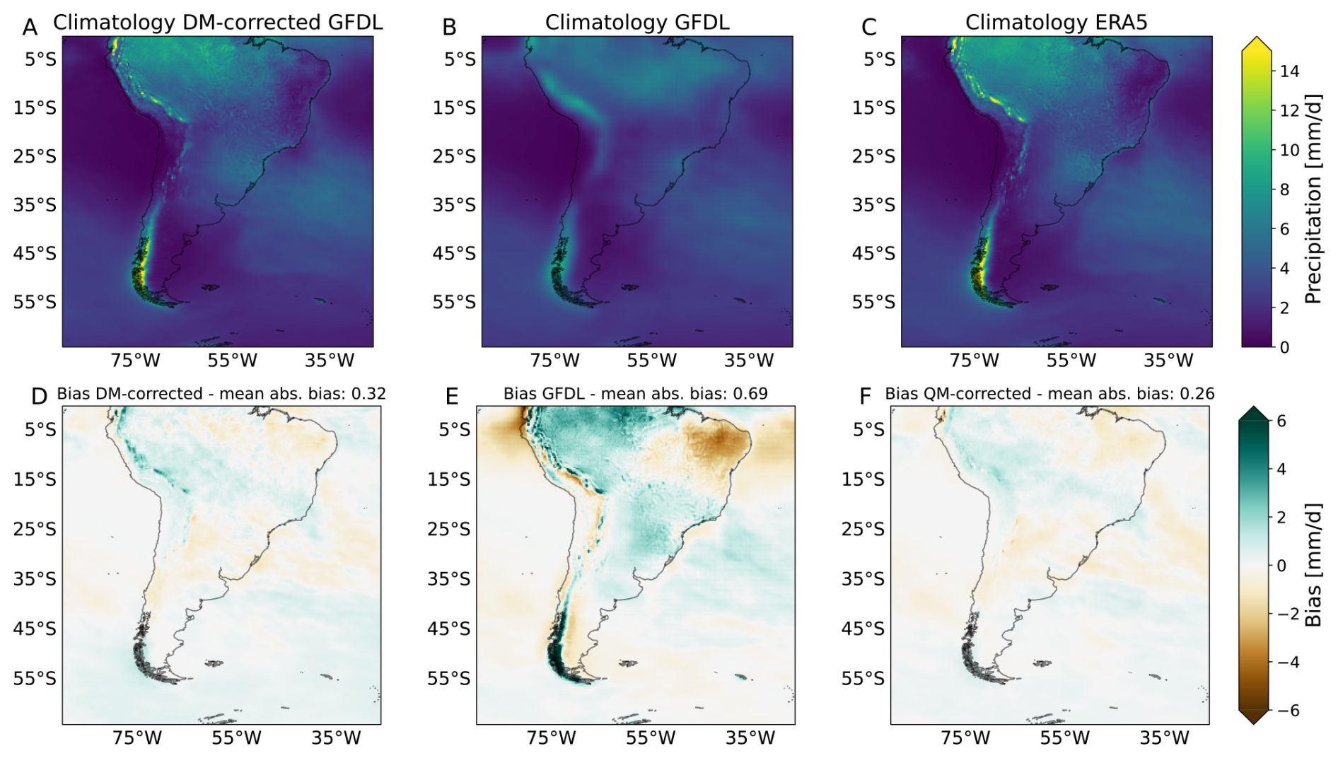
Figure 4 Comparison of climatologies and model biases. The first row shows the climatology of (a) the diffusion model-corrected GFDL at 0.25°, (b) the GFDL ESM4 model, upsampled to 0.25° and (c) the 0.25° ERA5 data. The second row shows the bias of the GFDL and the QM- and diffusion model-corrections, defined as the difference between long-term temporal averages of all validation samples. Specifically, the temporally averaged bias fields with respect to ERA5 are shown for (d) the diffusion model correction, (e) the uncorrected GFDL and (f) the QM correction. Results indicate a substantial improvement of our diffusion model (a) and the benchmark (c) over just upsampling GFDL to 0.25°. The absolute bias on top of each panel is given by the mean absolute value of the differences over the spatial and temporal dimension with respect to ERA5.

There are large differences between the GFDL and ERA5 data in small-scale patterns (Fig. 5a). The histogram of precipitation intensities (Fig. 5b) also confirms that the ESM is only really accurate for precipitation events up to 40 mm d⁻¹, after which the respective frequencies diverge. The latitudinal and longitudinal mean profiles (Fig. 5c and d) indicate the presence of regional biases.

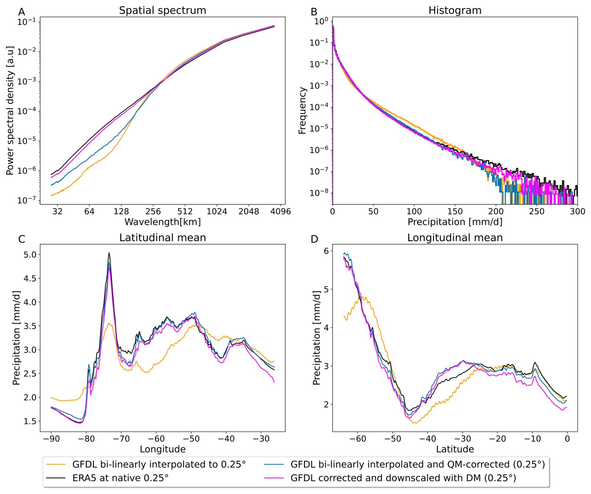
Figure 5 Evaluation of our diffusion model's performance for downscaling and bias correction. Comparison of GFDL (bilinearly upsampled to 0.25°) (orange) and ERA5 (black) to diffusion model-corrected GFDL (magenta) and QM-corrected GFDL fields (blue) as our benchmark. The Power spectral density (PSD) plot (a) shows that the diffusion model corrects the small-scale spatial details far better than our benchmark. The spectrum aligns very well with the high resolution ERA5 target data. The histograms (b) as well as the latitude (c) and longitude (d) profiles show substantial improvements compared to the uncorrected GFDL data.

Our framework demonstrates comparable skill to the QM-based benchmark in correcting the latitude and longitude profiles, for which QM is near optimal by construction (Fig. 5c and d). Comparing the histograms (Figs. 5b and S8) shows that our diffusion model is superior compared to the benchmark, strongly outperforming it for extreme values, in particular.

For the spatial patterns and especially the small-scale spatial features, the QM benchmark shows only slight improvements over the original GFDL data (Fig. 5a). The diffusion model is vastly superior in correcting these small-scale spatial patterns (Figs. 5a and 3) and almost completely removes the small-scale biases, as seen in the spatial PSD.

To verify that large-scale patterns are preserved by the diffusion model, we compute image similarity metrics between the low-pass-filtered embedded GFDL data and the low-pass filtered output of the diffusion model. The comparison yields an average structural similarity index value (SSIM, Wang et al., 2004) of 0.77 and a Pearson correlation coefficient of 0.90, verifying that large-scale patterns are well preserved by the diffusion model.

We also assess our model's performance on extreme precipitation events. For this, we use the R95p metric, which is defined as the total annual precipitation from wet days (PR > 1 mm d⁻¹) that exceed the 95th percentile of our reference period. The difference between the R95p values for the ERA5 and DM corrected GFDL (Fig. S9a), the ERA5 and QM corrected GFDL (Fig. S9b) and ERA5 and GFDL (Fig. S9c), demonstrate that the diffusion model effectively corrects the bias in extreme precipitation events, performing at least as well as the quantile mapping correction. To further test the model's performance on correcting characteristics of rainfall events in the tail of the distribution, we conduct a return-level analysis for extreme rainfall events (Fig. S10). We calculated the average return periods for both moderately extreme (>50 mm d⁻¹) and very extreme (>80 mm d⁻¹) events. The raw GFDL model has a significant wet bias, substantially underestimating the return periods (3.33 and 4.60 years) compared to the ERA5 reference (4.11 and 7.38 years). Our DM successfully mitigates this bias, yielding more realistic return periods of 4.18 and 7.98 years.

We show that the spatial correlation between the climatologies is improved through our method by computing the Pearson correlation between the temporally averaged fields. The Pearson correlation between ERA5 and GFDL climatology is 0.83, while the correlation between ERA5 and DM-corrected GFDL is 0.98, which is the same as that for the QM-corrected GFDL data. We also investigate how our DM captures the statistics of consecutive dry days (CDD) and consecutive wet days (CWD) compared to the QM benchmark and the raw GFDL (Fig. S11). Our diffusion model produces superior CDD (Fig. S12a and Fig. S12b) and CWD (Fig. S12d and e) statistics compared to our QM benchmark and GFDL, as shown in the difference plots of CDD/CWD.

Our method therefore accurately preserves the large-scale precipitation content, while successfully correcting small-scale structure of the precipitation fields, as well as statistical biases in histograms and latitude/longitude profiles (Fig. 5). Finally, we confirmed the temporal consistency of our model by analyzing autocorrelation (Fig. S13) and seasonal spell duration (Fig. S14). We further validated the robustness of our metrics over an extended validation period (1995–2014) (Fig. S15).

We also test our framework on a different region of similar size over South Asia. We choose the same GFDL dataset and keep the experimental setup and evaluation identical to the South American region. The setup for quantile mapping the South Asia GFDL data and creating the benchmark data is also the same. We retrained our DM on mapping embedded ERA5 data (over South Asia) to the original ERA5 data. The noising scale in this experiment is the same as for South America, as the PSDs for both regions diverge around the same spatial scale. The evaluation (Fig. S16) confirms that our DM successfully corrects precipitation biases in this new region and most notably outperforms the QM baseline in representing small-scale spatial features.

To further assess our framework's robustness, we conducted an additional experiment using a different ESM. We replaced the GFDL dataset with the MPI-ESM-HR model while keeping the experimental setup and evaluation protocol identical. The MPI and GFDL data diverge at a similar spatial scale in the PSD over the South American domain, allowing us to use the same noising scale hyperparameter s. Quantile delta mapping was applied in the same way as for the GFDL data. Consequently, our diffusion model did not require retraining and could be applied directly to the embedded MPI data at inference. Evaluation on our main metrics (Fig. S17) demonstrates our framework's ability to generalize to different ESMs. Our DM not only restores spatial variability across all scales significantly better than the QM benchmark (Fig. S17a), but also shows superior ability to reproduce the frequency of extreme precipitation events (Fig. S17b).

2.3 Evaluation of ensemble spread

One of the key strengths of our method lies in its capability to generate a diverse ensemble of downscaled and bias-corrected fields from a single condition. We therefore evaluate the ability of our diffusion model to represent and produce accurate estimates of uncertainty, a critical aspect for robust climate modeling and decision-making. We generate a 50-member DM ensemble by running the model 50 times, each conditioned on the same low-resolution ERA5 year, producing one-year trajectories. The corresponding high-resolution year serves as the ground truth. Our results demonstrate that the DM ensemble effectively reproduces the correct precipitation patterns, as shown by the close alignment between the ensemble mean and the high resolution ground truth of ERA5 over the annual cycle (Fig. S18). Probabilistic performance, evaluated using CRPS, highlights that the DM significantly outperforms a bilinear baseline, with lower mean CRPS values (0.76 mm d⁻¹ vs. 0.90 mm d⁻¹), as well as better temporally and spatially averaged CRPS (Fig. S19). Furthermore, we confirm that the DM ensemble produces well-calibrated uncertainty estimates with a spread-skill plot. Our model achieves near-perfect alignment with the 1:1 line, indicating an accurate representation of uncertainty (Fig. S20). For more details see Sect. S4.

2.4 Evaluation on future climate scenarios

Evaluating the performance of downscaling models is crucial for their application in climate impact studies under future climate scenarios. We assess our diffusion model's ability to preserve climate change signals in the underlying ESM simulations by applying it to a high-emission future scenario (SSP5-8.5). Figure 6 compares the relative climate change signal between the late 21st century (2081–2100) and the historical period (1995–2014) for annual mean and annual extreme precipitation. We find that our downscaled 0.25° fields successfully capture the mean precipitation change, closely matching the pattern and magnitude shown in the original 1° GFDL data (Fig. 6a and b). The diffusion model also robustly preserves the climate change signal for extreme precipitation indices, including Rx1Day (wettest day for each year) and R95p (Fig. 6c–f). The spatial patterns of change for the extremes are well-reproduced in the DM-corrected output compared to the original model data. Notably, slight differences are observed in the northwestern domain (Fig. 6c and e), where the DM-correction projects a slightly stronger increase in extreme events under SSP5-8.5. A slight increase in extremes aligns with the diffusion model's bias correction capabilities, reflecting its role in addressing the known under-representation of extreme precipitation in the original GFDL simulations.

Figure 6 Comparison of relative climate change signals. We compute the relative climate change signal between the late 21st century (2081–2100) under the GFDL SSP5-8.5 scenario and the historical GFDL period (1995–2014). In (a) and (b), we show that our diffusion model successfully preserves the mean precipitation climate change signal in the downscaled 0.25° GFDL fields, matching the change of the original 1° GFDL data. Positive values (red) indicate an intensification of precipitation, while negative values (blue) indicate reductions. In (c, d) and (e, f) we evaluate how well the DM-correction preserves the climate change signal for extreme events in historical and future scenarios. Both the Rx1Day (c, d) as well as R95p in (e, f) show that the DM-downscaling does preserve the climate change signal for extreme events. There are only slight differences over the north western part of our fields, where the DM-correction predicts more slightly more extremes for the SSP5-8.5 scenario. This is in line with the bias correction capabilities of the DM, correcting the under-representation of extreme precipitation in the original GFDL data.

Furthermore, we demonstrate that our conditionally trained diffusion model generalizes robustly to unseen future emission scenarios by accurately preserving regional precipitation trends without requiring retraining. We analyze the full annual mean precipitation timeseries from 2015 to 2100 over two representative regions, one exhibiting a strong negative trend and one with a pronounced positive trend (Fig. S21). For each region, we compare the annual mean precipitation from the original GFDL SSP5-8.5 data at 1° with the DM-corrected output at 0.25° resolution. The diffusion model consistently preserves the direction and magnitude of the trends found in the original GFDL data across the entire timeseries, for both the negative (Fig. S21, blue) and positive trend (Fig. S21, red) regions. This demonstrates the model’s ability to maintain physically meaningful long-term changes in precipitation, further supporting its generalization capability to future scenarios. Note that the absolute values do not have to coincide, as our model corrects the bias and hence the numerical values. Our model can generalize to unseen climates, preserving the trends, since there is no decrease in performance during inference on GFDL SSP5-8.5 data. Note that our set-up generalized to unseen climate scenarios without any external constraints. The reason why our model preserves trends well is likely given by the fact that the trend is dominated by the large-scale patterns and our model learned to rely on the large-scale patterns of the condition and only generates small-scale patterns.

3 Discussion

We introduced a framework based on generative machine learning that allows both bias correction and downscaling of Earth system model fields with a single diffusion model. We achieve this by first mapping observational fields and ESM data to a shared embedding space and then applying the learned inverse of the observation embedding transformation to the embedded ESM fields. We learn the inverse transformation with a conditional diffusion model. Although the underlying observational and ESM fields are unpaired, our framework allows for training on paired data (between observations and embedded observations, see above) and therefore any supervised machine learning method can be adopted to the task, which allows for more flexibility. Supervised methods are often superior in performance and more natural for the downscaling application. The diffusion model is trained on individual samples and has successfully learned to reproduce the statistics of observational data. For the observational ground truth, we chose the ERA5 reanalysis, and for the ESM data to be corrected and downscaled, we chose fields from GFDL-ESM4.

We demonstrated our framework's robustness and generalizability in two additional experiments (Sect. 2.2). When applying the model to a new geographical region in South Asia with the same ESM, the DM requires retraining to adapt to the new regional characteristics. In contrast, when applying the framework to an entirely different ESM (MPI-ESM) over the South American region, the core DM did not need to be retrained since the same noising scale hyperparameter could be used. For different ESMs a new noising scale hyperparameter could be necessary, requiring retraining of our DM with a different noising scale; however this depends on the choice of the spatial scale below which bias correction is desired, and for comparable outputs, we recommend to keep the noising scale s fixed for different ESMs. For example, to correct multiple ESMs at once, one can use the most heavily biased model to select the noising scale. A single diffusion model can then be trained to correct all ESMs at once, saving significant computational resources during inference. In general, we expect that many ESMs (like the MPI and GFDL model we use) will have similar spatial scales up to which they can capture realistic spatial precipitation features, because they have a similar resolution and have similar limitations from parameterization schemes. In all cases, readjusting the computationally inexpensive Quantile Delta Mapping (QDM) is a required step in the embedding process. The results will also depend on the specific quantile mapping scheme, QDM is chosen to preserve trends.

Our diffusion model corrects small-scale biases of the ESM fields, while completely preserving the large-scale structures, which is key for impact assessments, especially with regard to extremes and local impacts in terms of floods or landslides. The diffusion model performs particularly well for extreme events where traditional methods struggle. The method improves the temporal precipitation distribution at the grid cell level and surpasses the state-of-the-art approach (quantile mapping) in correcting spatial patterns. The downscaling performance has also been shown to be excellent. The diffusion model manages to generate small-scale details for the low resolution ESM data, that match those of high resolution observations. Our model preserves relevant information from the large scales, such as trends and extremes, and generates bias corrected and downscaled precipitation fields with adequate uncertainties.

We show that our method is robust in the out-of-distribution setting of downscaling and bias-correcting the SSP5-8.5 future emission scenario. It is critical for impact assessments that our model is able to accurately preserve the climate change signal of the original SSP5-8.5 data.

A key innovation of our approach is the embedding strategy, which makes the training process independent of the source ESM (apart from a single data-dependent hyperparameter setting the spatial scale below which the fields are corrected), which not only allows the framework to be flexibly applied to downscale and bias-correct a wide range of ESMs but also allows it to be used with different state-of-the-art machine learning backbone models. Another key advantage of our framework is its data efficiency. In our conditional approach the model only needs to learn how to generate small-scale features given the large-scale ones. The task is considerably less demanding than that of unconditional models (Hess et al., 2025), which must learn the entire data distribution from scratch during training. This data efficiency makes our method applicable to datasets with shorter record lengths than ERA5, such as newer observational products.

Indeed, comparing results for generated climatologies between our conditional DM and the unconditional consistency model (CM) by Hess et al. (2025), it becomes apparent that the CM struggles to learn the target distribution accurately, leading to blurring (Fig. S2) that would hinder applications for impact assessments.

Our method is not specific to ERA5 and GFDL because the training of the diffusion model does not directly depend on the ESM choice. A specific ESM choice will only modify a hyperparameter in the embedding transformations f and g. This, however, requires almost no fine-tuning, as the temporal frequencies can always be matched with quantile mapping. The only parameter that might change for different datasets and use cases is the amount of noise that is added to the observational and ESM datasets. We choose the amount of noise such that the PSDs of the observational ground truth and the ESM fields align beyond a certain scale. This means that we have complete flexibility in deciding which patterns we want to preserve and which we want to correct. This is a major advantage over existing GAN based approaches.

We can decrease the level of detail that is preserved by the diffusion model through increasing the amount of noise added in the transformations f and g. The amount of noise added is directly proportional to the freedom the diffusion model has in generating diverse outputs and inversely proportional to the model's ability to preserve large-scale patterns.

The downscaled and bias corrected fields will automatically inherit time consistency between different samples up to the noising scale. This means that ESM fields showing two successive days will still look like two successive days after the correction. Future work could build a video diffusion model that inputs and outputs full time series instead of single frames, in order to guarantee time consistency across all scales.

We focused on precipitation data over the South American continent, because of its heavily tailed distribution and the pronounced spatial intermittency. Especially at small scales, precipitation data is extremely challenging to model and therefore serves as a reasonable choice to show the framework's capabilities in a particularly difficult setting. Regional data is chosen due to computational constraints, yet the diverse terrain of our study region, encompassing land, sea, and a wide range of altitudes, enables robust testing of the downscaling and bias correction performance, also given the substantial biases of the GFDL model in this region. We also conducted additional experiments for another region over South Asia, and using another ESM, namely the MPI-ESM-HR, in order to confirm the generality of our approach. The extension to global scales is straightforward and requires no major changes in the architecture. We intend to include more variables in a consistent manner on a global scale in future research. Optimizing the inference strategy, with speedup techniques such as distillation (Luhman and Luhman, 2021), to decrease the sampling time will prove helpful in this context. As for any ML model, the ability to generate the rarest extremes is limited by their frequency in the training data. Our conditional approach helps mitigate this to some extent by inheriting the large-scale patterns for these events directly from the ESM.

It is straightforward to extend our methodology to downscaling and bias correction of numerical or data-driven weather predictions on short- to medium-range or even seasonal temporal scales. This would not require any fundamental changes to the architecture. This would, however, require a target dataset with sufficiently high resolution. The ability of the diffusion model to not disturb the temporal consistency between samples can be useful in this scenario. Future work could then focus on extending this model to a multivariate setting, which would be essential for weather prediction and for assessing physical consistency between variables.

4 Materials and methods

4.1 Data

For the study region, we focus on the South American continent and the surrounding oceans. Specifically, the targeted area spans from latitude 0° N to 63° S and from longitude −90° W to −27° E. For the ablation study of the South Asian region, we selected an area from 0.75 to 64.5° N latitude and from 42 to 105.75° E longitude. The training period comprises ERA5 data from 1 January 1992 to 1 January 2011. The range of years included for the evaluation on ERA5 and GFDL spans from 2 January 2011 to 1 December 2014. Additionally, an extended 20-year window (1995–2014) is used for analyses requiring greater statistical robustness.

ERA5

ERA5 (Hersbach et al., 2020) is a state-of-the-art atmospheric reanalysis dataset provided by the European Center for Medium-Range Weather Forecasting (ECMWF). Reanalysis refers to the process of combining observations from various sources, such as weather stations, satellites, and other instruments, with a numerical weather model to create a continuous and comprehensive representation of the Earth's atmosphere. We use the daily total precipitation data at 0.25° horizontal resolution as the target for the diffusion model.

GFDL

The climate model output is taken from a state-of-the-art ESM from Phase 6 of the Coupled Model Intercomparison Project (CMIP6), namely GFDL-ESM4 (Dunne et al., 2020). We abbreviate the model with GFDL throughout the paper. The dataset contains daily precipitation data of the first ensemble member (r1i1p1f1) of the historical simulation (esm-hist). The data is available from 1850 to 2014, at 1° latitudinal and 1.25° longitudinal resolution and a daily temporal resolution.

GFDL-ESM4 (Dunne et al., 2020) SSP5-8.5 represents a high-emission future pathway. We use daily-resolution data from the CMIP6 archive, provided at 1° latitude and 1.25° longitude spatial resolution, covering the period from 2015 to 2100.

MPI

For our ablation study, we repeat our experiments for the MPI-ESM HR model (Gutjahr et al., 2019). We abbreviate MPI-ESM-HR with MPI in the paper. The data has 0.9375°×0.9375° spatial resolution. We use daily data from 1992 to 2014 using data from 1992–2011 for training and 2011 to 2014 for inference.

Benchmark dataset

In order to benchmark our method, we first apply bilinear interpolation to increase the resolution of the GFDL fields from 1 to 0.25°. After that, we apply quantile delta mapping (Cannon et al., 2015) to fit the upsampled GFDL data to the original 0.25° ERA5 data. QM is fitted on past observations and can then be used to correct the statistics of any (past/present) ESM field towards that reference period. We use quantile delta mapping (QDM) and chose the ERA5 training period from 1 January 1992 to 1 January 2011 as the reference period to fit the GFDL to ERA5. The benchmark dataset to evaluate our approach is then constructed by applying QM to the GFDL validation period (2 January 2011 to 1 December 2014). Some analyses required a longer evaluation period (1995–2014). To create a fair benchmark for these specific cases QDM was also recalibrated, it was both fitted and applied using data exclusively from this 1995–2014 window. For the SSP5-8.5 data, we use the 1995 to 2014 period of ERA5 as reference data and the historical GFDL data as the model input to fit the QDM. We then apply this mapping to the full time period of the GFDL SSP5-8.5 data (2015–2100).

Data pre-processing

The units of the GFDL data and MPI data are kg m⁻² s⁻¹, and for ERA5 m h⁻¹. For consistency, both are transformed to mm d⁻¹.

Our pre-processing pipeline consists of:

• Only GFDL: rescaling the original 1°×1.25° GFDL data to 1×1° (64×64 pixel).

• Only MPI: rescaling the original 0.9375°×0.9375° GFDL data to 1×1° (64×64 pixel).

• Add +1 mm d⁻¹ precipitation to each value in order to be able to apply a log-transformation to the data.

• Apply the logarithm with base 10 in order to compress the range of values.

• Standardize the data, i.e. subtract the mean and divide by the standard deviation to facilitate training convergence.

• Transform the data to the range [−1, 1] to facilitate the convergence of the training.

An ablation study (Fig. S22) confirms the choice of our precipitation pre-processing pipeline, showing that omitting the log-transformation or the final range scaling leads to spectral discrepancies or distributional biases. As part of the transformation g, the 1° GFDL data is bilinearly upsampled. This and the downsampling and upsampling of ERA5 data, which is part of f, are already done during pre-processing. The downsampling of 0.25° ERA5 data (256×256 pixel) to 1° (64×64 pixel) is done by only keeping every fourth pixel in each field. For the just mentioned upsampling, we apply bilinear interpolation to increase the resolution from 1 to 0.25°. Note that bilinear interpolation to 0.25° does not increase the amount of information in the images compared to the 1° fields. After preprocessing the data as described, the embedding transformation f is applied. The diffusion model is trained with the preprocessed f(ERA5) as a condition and the original 0.25° ERA5 data as a target. Before we apply the embedding transformation g we first pre-process the 1° GFDL data by applying quantile delta mapping (QDM, Cannon et al., 2015) with 500 quantiles. The bilinear upsampling is then used to increase the resolution to 0.25×0.25° (256×256 pixels). The preprocessed data are used as input to the embedding transformation g. The corresponding output serves as the condition during the inference process of the diffusion model

4.2 Embedding framework

Our framework introduces transformations f and g that map OBS and ESM data to a shared embedding space $f:{\mathbf{V}}^{\mathrm{obs}}\to {\mathbf{V}}^{\mathrm{emb}}$ and $g:{\mathbf{V}}^{\mathrm{esm}}\to {\mathbf{V}}^{\mathrm{emb}}$. The goal is to do bias correction and downscaling of ESM fields, i.e., to obtain samples from the conditional distribution $\mathit{\omega }=p\left(\mathrm{OBS}\right|\mathrm{ESM})$. Training a conditional model to approximate this distribution directly is not possible because OBS and ESM are unpaired. Therefore, we will train the model without the ESM data, only using OBS data and utilize a trick to enable transfer learning and inference on the ESM data. We apply transformations on ESM and OBS such that the resulting datasets are similarly distributed and therefore allow for generalization. The arrows in the diagram of Fig. 1 show that we can represent the mapping that achieves the bias correction and downscaling as $\mathit{\omega }=f^{-\mathrm{1}}\circ g$. Our idea is to approximate f⁻¹ with a neural network $f^{-\mathrm{1}}\approx \mathit{ϵ}$. We chose a conditional diffusion model (DM), denoted by the conditional distribution p(OBS|f(OBS)), to approximate $f^{-\mathrm{1}}=\mathrm{DM}$: V^emb→V^obs. The diffusion model (Fig. 1c) is only trained on pairs (OBS,f(OBS)). The shared embedding space allows us to evaluate the trained model on ESM embeddings p(OBS|g(ESM)), as all embeddings are identically distributed.

Constructing the embedding space

The goal of f and g is to map OBS and ESM to a shared embedding space, where f(OBS) and g(ESM) are identically distributed (Fig. 1). To achieve this, both embedded datasets need to be unbiased towards each other. OBS and ESM are biased towards each other in terms of statistical biases between distributions and biases between small-scale patterns visible in the spatial power spectral density (PSD) (Fig. S4a).

As mentioned earlier, the input for the embedding transformation f is 0.25° ERA5 data, which is first preprocessed, then downsampled and upsampled. The input to the embedding transformation g is the preprocessed and upsampled 0.25° GFDL data. By first downsampling ERA5 to 1° and then upsampling it to 0.25° we ensure that the fields match the information content of the original 1° GFDL fields.

To remove small-scale pattern bias, we apply a noising procedure analogous to the forward diffusion process as part of f and g. Gaussian noise contains all frequencies in equal measure and the Fourier transform of Gaussian noise is itself Gaussian noise, so its power must be equal across all frequencies in expectation. The power spectrum of pure Gaussian noise corresponds to a horizontal line in the spectrum of Fig. 2a, reflecting the fact that it contains all frequencies in equal amounts. Adding noise to an image results in a hinge shape in the PSD of the noisy images (Fig. 2a, c and d). Increasing the variance of the noise increases its power and, as a result, its PSD will shift upward. Adding noise hence acts as a low-pass filter, while the variance of the added noise determines the cut-off frequency. Increasing variance leads to higher cut-off points as the power of the noisy frequencies increases. Both ERA5 and GFDL data are noised up to the cutoff frequency, denoted by s. The scale s is determined by the point where ERA5 and the ESM data (in our case GFDL) start to disagree in their spatial PSDs (Fig. 2), i.e., the intersection between the two. Adding noise in this way ensures that f(ERA5) is unbiased compared to g(GFDL) in the PSD by erasing all information beneath s. In our implementation, the transformations f and g utilize the same cosine scheduler as the forward diffusion process to add Gaussian noise to the data. ERA5 data undergoes 50 noise steps within f, while g applies the same 50 noise steps to the GFDL data. We ensure that the observational and ESM data have aligned distributions by incorporating Quantile Mapping (QM) directly into the transformation g. It only needs to be included in g. The quantile-mapped and bilinearly downscaled data is then noised as described above, as part of the embedding transformation. It is important to clarify that QM is not included because the diffusion model is unable to do bias correction. QM is only used as a tool in our framework to ensure that in the embedding space f(ERA5) and g(GFDL) are identically distributed, such that g(GFDL) can be used for the inference of the diffusion model.

Determining the noising scale

The choice of the spatial scale s influences up to which scale we correct the spatial PSD. We note that the PSD shows spectral distributions normalized to 1; therefore, we can still observe slight changes above s when small-scale patterns are corrected. The point s is a hyperparameter chosen before training and purely depends on the datasets ESM and OBS and can be adjusted to the specific needs in a given context and task.

In the extreme case, where s is maximal, the conditional images will contain pure noise (Fig. 2a). In this case, the diffusion model is equivalent to an unconditional model. As an unconditional model, the diffusion model will correct all biases at all spatial scales, however, at the expense of completely losing any paring between the condition and the output. We chose s to be at the intersection of the ERA5 and GFDL spectrum around 512 km (Fig. 2b). Thereby, we trust in the ESM's ability to model large-scale structures above the point s, which we do not want to correct with the diffusion model.

4.3 Network architecture and training

The general architecture of our diffusion model DM consists of a Denoising Diffusion Probabilistic Model (DDPM) architecture (Ho et al., 2020) conditioned on low resolution images. For details about diffusion models and conditional diffusion models, see Sect. S1.1 and S1.2 in the Supplement. We employ current state-of-the-art techniques to facilitate faster convergence and find the following to be important for convergence and sample quality (Saharia et al., 2022b): The memory efficient architecture, “Efficient U-Net”, in combination with dynamic clipping and noise conditioning augmentation (Ho et al., 2022) turned out to be effective for our relatively small dataset. We adopt the Min-SNR (Hang et al., 2023) formulation to weight the loss terms of different timesteps based on the clamped signal-to-noise ratios. The diffusion model architecture utilizes a cosine schedule for noising the target data and a linear schedule for the condition during noise condition augmentation with 100 steps each. The diffusion model is trained to do v-prediction. The U-Net follows the $\mathrm{64}\times \mathrm{64}\to \mathrm{256}\times \mathrm{256}$ Efficient U-Net architecture (Saharia et al., 2022b). The diffusion model has approximately 730 million trainable parameters and is trained for 100 epochs using the ADAM optimizer (Kingma and Ba, 2015) with a batch size of 2 and a learning rate of $\mathrm{1}\times {\mathrm{10}}^{-\mathrm{4}}$. Note that in the case of Fig. S4, where the inference data is also embedded OBS data and there is no ESM data present, the model performs better when being trained and evaluated with 1000 denoising steps, instead of the 100 steps that we used in all our experiments that include ESM data. The model with 100 steps is superior in training and inference speed and also in correcting the histograms, when correcting ESM data. We also compared the effect of not adding noise (Sect. S2.1) and the effect of not applying QM (Sect. S2.3) as shown in Figs. S23–S27, as well as different noise choices (Sect. S2.2, Fig. S28) during both training and inference.