Development of an under-ice river discharge forecasting system in Delft-Flood Early Warning System (Delft-FEWS) for the Chaudière River based on a coupled hydrological-hydrodynamic modelling approach

Year-round river discharge estimation and forecasting is a critical component of sustainable water resource management. In cold-climate regions such as Canada, this task is complicated by dynamic river-ice conditions which alter channel hydraulics and render open-water rating curves invalid. Some methods such as backwater-adjusted rating curves and ice thickness-based rating curves have been developed. However, these methods are site specific and subjective to human judgement. It is therefore an active field of research and development. The current study develops and assesses the performance of a river ice forecasting system for the Chaudière River in Quebec based on coupled hydrologic-hydraulic modelling approach within the Delft Flood Early Warning System (Delft-FEWS) platform. The current configuration of the system integrates (i) meteorological products such as the Regional Ensemble Prediction System (REPS); (ii) a hydrological module implemented through the HydrOlOgical Prediction LAboratory (HOOPLA), a multi-model based hydrological modelling framework; and (iii) hydraulic module implemented through a 1D steady and unsteady HEC-RAS river ice models. The system produces ensemble forecasts for discharge and water level and provides flexibility to modify various dynamic parameters such as discharge timeseries, and ice properties. Performance of the coupled modelling approach was assessed against “Perfect Forecast” for selected winter events between 2020 and 2023 using the root mean square error (RMSE) and percent bias (PBias) metrics. The hydrologic module of the system consistently underestimated the under-ice discharges. This can be explained by the inherent uncertainty in the under-ice discharge estimates used as observations as well as uncertainty in the model states. The hydraulic module had an RMSE between 0.1–0.5 m. The higher error in RMSE can be attributed to the uncertainty in the ice thickness estimates at one of the stations. The PBias analysis of the hydraulic module also confirmed that the forecasted discharges were under-estimated by the hydrologic module.

1 Introduction

Water resource management agencies across Canada have developed forecasting systems for efficient management of water resources throughout the year; however, the winter season presents a special challenge to all agencies when the natural streams are affected by an ice cover, rendering the under-ice discharge estimates subjective to expert judgment, interpolations and theoretical methods (Turcotte and Morse, 2017). These practices introduce significant uncertainty and inaccuracy in the winter records (Dahl et al., 2019). Moreover, most of these methods are passive in nature i.e., the winter flow records are not produced in real-time. Some agencies produce preliminary estimates and short-term discharge forecasts, but final validated values are produced and published at the end of the season.

River ice forecasting is essential to flood management during winters for several basins across Canada (Pietroniro et al., 2021). In winters, flooding is usually associated with the formation or release of ice jams and can occur even at discharges much lower than those in open water conditions (Beltaos and Prowse, 2001; Beltaos, 2021). Apart from flood risk assessment, river ice forecasting also provides essential information for water resources management especially for the hydropower sector. River ice modelling is a critical component of any forecasting system developed in cold climate regions, as it considers the influence of the ice cover on the flow dynamics and flooding events (Montero et al., 2023). River ice conditions are dynamic and can change rapidly over a short time period, hence, it remains an active area of research and development (Belvederesi et al., 2022).

Accurate estimation of under-ice discharge has remained a challenge for the river ice community and forecasting agencies. Therefore, various attempts have been made to come up with methods or techniques to improve practices and procedures. In Canada, Water Survey of Canada (WSC) assumes major responsibility for this task. The WSC has established methodologies for varying conditions and sites. This comprises of collecting preliminary data through hydrometric stations, estimating instantaneous discharge from rating curve or index velocity method (Healy and Hicks, 2004). At some sites rating curves based on ice conditions have also been developed. The WSC also conducts direct measurements; however, they are low in frequency. At the end of the season a post processing of the entire winter dataset is performed by WSC technicians using methods such as recession constant, graphic interpolation, comparison of hydrograph, and backwater adjustment models. Other agencies across Canada have adopted similar practices comprising of handful of direct measurements and post processing instantaneous data (Turcotte and Morse, 2017).

The Nordic countries (Finland, Sweden, Norway and Iceland) also experience river ice conditions during the winters and face similar challenge in discharge measurement and estimation during the winter. The study conducted by Turcotte and Morse (2017) also summarized the practices observed in Nordic regions for under-ice discharge estimation. The agencies responsible for collection and distribution of hydrometric data follow a similar approach which consists of conducting a few discharge measurements during the ice-covered period and later estimating the hydrograph based on comparison with hydrographs from catchment with similar hydrology but no ice conditions, or the one produced through hydrological modelling. The experience of the operator/technician responsible for publishing the under-ice discharge data has proven to be essential for data quality.

Hydrological modelling approaches have been tested for the simulation of winter discharge (Hamilton et al., 2000; Turcotte et al., 2005; Levesque et al., 2008). Hamilton et al. (2000) applied a conceptual hydrological model, a variant of the Hydrologiska Byråns Vattenbalansavdelning (HBV) model developed at the Swedish Meteorological and Hydrological Institute (SMHI) by Bergström (1995), for simulating daily discharge estimates in M'Clintock River watershed, Yukon. The HBV model is a conceptual hydrological model that consists of routines describing snow accumulation and melt, soil moisture accounting, runoff and routing. The model runs on precipitation, temperature and potential evapotranspiration as inputs and can be considered as a semi-distributed hydrological model since the basin is divided into different zones based on altitude, and vegetation (Zhang and Lindström, 1997). The study by Hamilton et al. (2000) concluded that hydrological modelling produced reasonable estimates for winter discharge but failed to capture discharge variability over the season. Turcotte et al. (2005) compared the performance of hydrological modelling to a data driven neural network model. Their study found that both hydrological model and the Neural Network model performed equally well before snowmelt started influencing the streamflow during the winters and concluded that the skill of hydrological modelling could be improved if winter streamflow gauging data is used for model calibration. A study by Levesque et al. (2008) also showed potential of hydrological modelling for winter discharge estimation where a process based Soil and Water Assessment Tool (SWAT) model was calibrated for streamflow estimation in two small catchments in Southern Québec. Hicks and Healy (2003) investigated the viability of using hydraulic modelling (gradually varied flow conditions) to determine under-ice discharge, based on data obtained from the Mackenzie River and the Athabasca River. The study found that hydraulic modeling has the potential to provide a substantial increase in accuracy compared to conventional approaches, with maximum error of less than 3 % in discharge determined by this method. However, the authors cited a potential limitation to this approach was the estimation of the ice cover thickness. Ice cover thickness is not uniform along a river as well as across a cross section. This may induce some degree of uncertainty in this method of estimating under-ice discharge.

The interaction of ice with river hydraulics is a complex process that depends on a number of factors such as surface ice concentration, the type of the cover, and the hydraulic regime of the river (Montero et al., 2023). Research into these processes have lead to the evolution of several river ice models (e.g., RIVICE, River1D) describing different river ice processes such as thermal exchange, ice formation processes, and ice jams hydraulics (Blackburn and She, 2019; Rokaya et al., 2022). More recent studies have aimed to develop simplified, depth-averaged approaches for characterizing under-ice river hydraulics. Koyuncu et al. (2024) developed a Shiono-Knight model (SKM) based method to reconstruct under-ice depth-averaged velocity profiles based on channel geometry and a single velocity measurement. Souri et al. (2025) propose depth-integrated momentum models derived from Reynolds-averaged Navier Stokes (RANS) equations to predict depth averaged lateral flow velocity distributions based on geometric and hydraulic parameters. Although these models enhance our comprehension of various river ice processes, their data-intensive nature for calibrating various parameters limits their applicability in operational forecasting systems.

Operational forecasters prefer to adopt less complex modelling approaches and simulate river hydraulics under the assumption of a fully developed ice cover. This approach is practical from the operational viewpoint and is less data and computation intensive as compared to a process-based modelling. HEC-RAS (Brunner, 2016) is a hydraulic modelling software that provides a suitable option since it can simulate simple ice covers and ice jams hydraulics. It is widely used by hydrotechnical engineers, and is available open source with a user friendly interface and documentations (Beltaos and Tang, 2013). For simple ice cover hydraulic modelling, HEC-RAS has limited data requirements mainly ice thickness and under ice roughness at each cross-section which makes it applicable in an operational setting (Montero et al., 2023).

Recently coupled modelling approaches are gaining popularity among researchers in field of flood forecasting (Mai and De Smedt, 2017; Liu et al., 2018; Bessar, 2021; Rokaya et al., 2022). This approach consists of connecting different types of models together to create an integrated modelling chain for forecasting floods. Usually this consist of a hydrological model serving as a streamflow prediction layer and subsequently informing a hydraulic model which then maps out flooding extent. Nevertheless, more layers of complexities can be added to the approach such as coupling meteorological prediction systems (MPS) to hydrological systems (Zhijia et al., 2004; Cattoën et al., 2016). Within these systems another degree of sophistication is added by adopting the ensemble approach that helps mitigate uncertainties (Bessar et al., 2021) arising from different sources in the modelling chain and communicate the range of possible outcomes, providing decision-makers with a more comprehensive understanding of the associated risks.

Hydrological models are commonly employed for streamflow forecasting, and a well calibrated hydrological model can provide relatively accurate streamflow forecasts under normal operational conditions (Girons Lopez et al., 2021; Piazzi et al., 2021). However, river ice conditions pose many challenges that cannot be incorporated into hydrological models such as hydraulic backwater effects of the ice cover's roughness (Das and Lindenschmidt, 2021), channel storage due to jamming, restricted flows (Beltaos, 2014), abstraction of water from the system owing to ice formation etc. (Prowse and Beltaos, 2002). Coupling a hydrological model with a hydraulic model offers a comprehensive modelling approach under river ice conditions. This framework provides a feedback mechanism between the natural water cycle and the channel hydraulics, allowing the utilization of all data sources i.e. meteorology, hydrological states, and finally hydraulic controls (i.e. stage) to make fairly accurate discharge estimates and forecasts in near real time.

Despite recognizing the impact of river ice on water resource management and ice jam related flooding, operational forecasting systems that integrate a river ice modelling component are rare (Montero et al., 2023). A recent example of such an integration is the lower Churchill River in Labrador, where river ice modelling is embedded into an operational forecast. The system forecasts flows on the river using the hydrological model HEC-HMS and estimates water levels using the hydraulic models HEC-RAS (for open water) and RIVICE (for ice conditions) (Lindenschmidt et al., 2021). This system operates in deterministic mode without the application of data assimilation which makes it susceptible to forecasting errors and uncertainties. Moreover, it does not describe any framework to update hydraulic parameters such as the under-ice roughness which evolves over the season. The current study builds up on preliminary efforts of Montero et al. (2023), that laid down the foundation for a river ice forecasting testbed, to investigate the potential of an ensemble based coupled hydrologic and hydraulic modelling approach to address the winter hydrometry challenge in an operational forecasting setting. Hence the study has two main objectives: (i) to demonstrate the capabilities of an ensemble based coupled hydrologic-hydraulic modelling operational forecasting system, (ii) to assess the functionality and performance of this system for forecasting under-ice discharge and associated water levels using some selected events. The current study also implements data assimilation for improved forecasting performance. The paper first describes the case study area and available data. It then provides a description of components of the operational system and its capabilities to integrate different input data sources to each model. Finally, the performance of the system is demonstrated based on several under-ice hydrologic events observed in the winters between 2020–2023.

2 Watershed and data

2.1 Description of watershed

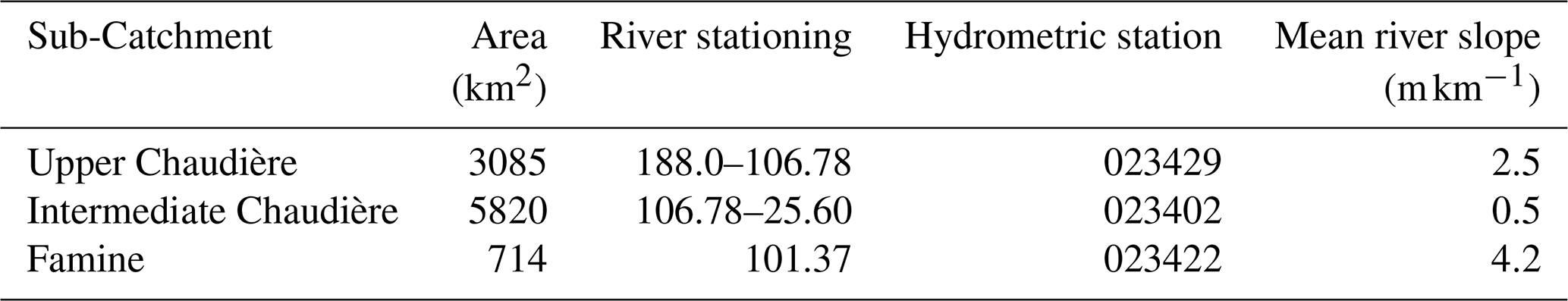
The description of the watershed for this study has been presented in Montero et al. (2023). A short summary is presented here. The Chaudière River basin is selected as the study basin. It is located South-East of Québec City, Canada. The river has its source at Mégantic Lake and drains into the Saint Lawrence River near the Town of Lévis, with a total river length of 188 km and a total watershed area of 6694 km². Based on the hydrometric station network, the Chaudière River basin was divided into three sub-catchments: (i) Upper Chaudière, (ii) Intermediate Chaudière, and (iii) Famine. This subdivision facilitated the representation of distinct hydrologic response units and provided the necessary boundary conditions for the hydraulic model. Table 1 (Montero et al., 2023) provides the main characteristics of the three sub-catchments. Figure 1 presents the study site.

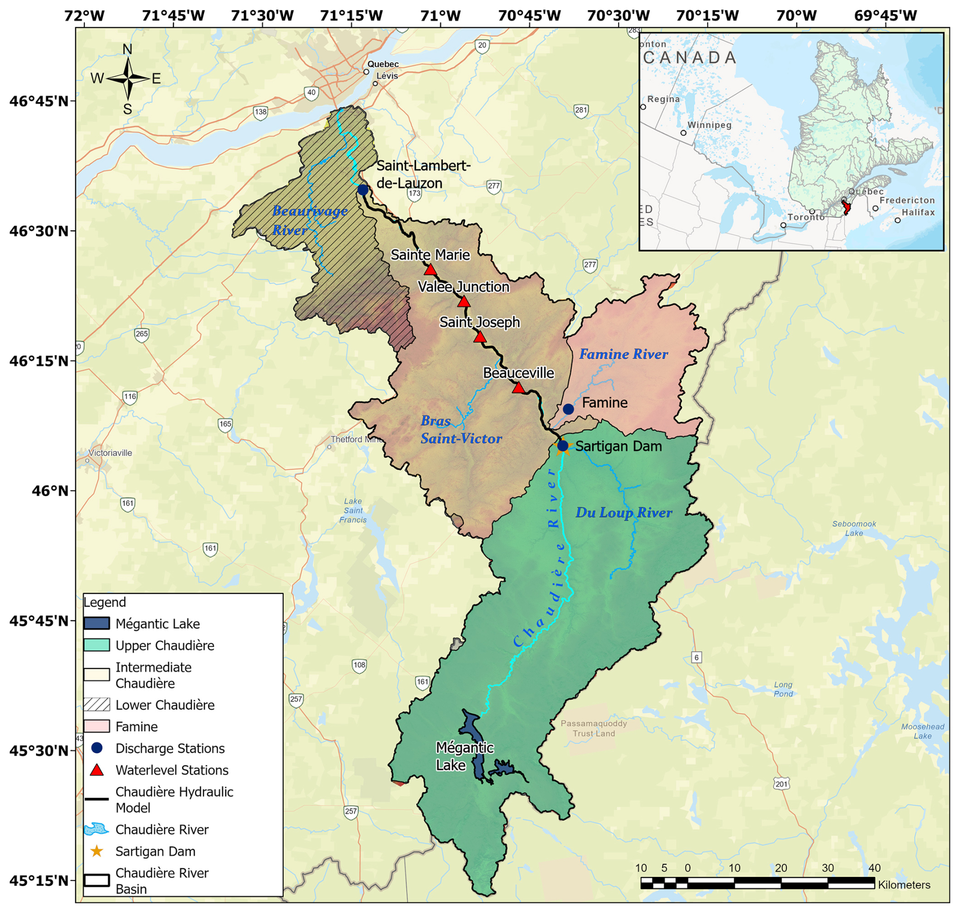
Figure 1 Chaudière River basin and its sub-catchments based on hydrometric control points (blue dots). The hydraulic model is developed for the Intermediate Chaudière between Sartigan Dam and Saint Lambert-de-Lauzon (black line). Hatched portion in the map shows the Lower Chaudière sub-catchment that is not included in this study.

Table 1 Characteristics of the Chaudière Basin sub-catchments.

The Upper Chaudière river reach is defined from its origin at Mégantic Lake (Ch. 188 km) up to the Sartigan Dam (Ch. 106.78). The river reach is relatively steep with an average slope of 2.5 m km⁻¹. A major tributary to the Chaudière River in this reach is the River Du Loup. Ice jam floods are common in the Intermediate Chaudière where the river profile is flatter and exhibits several meanders, islands and bridges (Montero et al., 2023). The Comité de bassin de la rivière Chaudière (COBARIC) operates four water level monitoring stations along the Intermediate Chaudière located near major urban communities (labeled as COBARIC stations in Fig. 1). These locations are Beauceville (ch. 87.5 km), Saint Joseph (Ch. 71.5 km), Valée Junction (Ch. 61.8 km) and Sainte Marie (Ch. 52.1 km) (Montero et al., 2023). The lower Chaudière (Chainage 25.60–0.0 km) is not included in this study since this section is steep and does not pose any serious ice jam flooding hazards. A detailed description of the Chaudière river's ice characteristics can be found in Ghobrial et al. (2023).

The Famine River is a major tributary to the Chaudière River with a catchment area of 714 km² and a total river length of approximately 54 km. The river has an average slope of 4.2 m km⁻¹. It joins the Chaudière River in the town of Saint-Georges, in Beauce.

The climatic regime dominant in Southern Québec is classified as humid continental (Dfb) according to the Köppen classification (Kottek et al., 2006). The average monthly temperatures in the Chaudière River basin show a high degree of seasonal variation with below freezing temperatures (average −6 °C and min −12.6 °C) between November-March and moderate temperatures (average 18 °C, high 25 °C) during the summers (Montero et al., 2023). The average annual precipitation is estimated to be 1031.5 mm shared between rain (824.9 mm) and snow (202.6 mm) (MELCCFP, 2023). Precipitation analysis of the catchment does not show significant variation between different months however, between June and August the intensity of precipitation is slightly higher (Montero et al., 2023). The hydrological regime for the catchment can be classified as nivo-pluvial since the spring flood caused by snowmelt and precipitation is dominant, followed by flooding in autumn season due to excess rainfall (Ricard et al., 2023).

2.2 Data

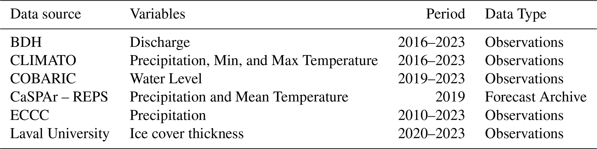
The data used in this study is presented in Table 2. It can be broadly classified into three main categories i.e. (i) Meteorological data, and (ii) Hydrometric data and (iii) Geographic data. These three different types of datasets were incorporated into the Delft-FEWS system. The meteorological dataset consists of observed and forecasted precipitation and temperature timeseries. The meteorological observations were extracted from the CLIMATO database system, managed by the Ministère de l'Environnement, de la Lutte contre les changements climatiques, de la Faune et des Parcs (MELCCFP, 2022), as well as from the Meteorological Service of Canada (MSC) Open Data Server (ECCC, 2025), managed by Environment and Climate Change Canada (ECCC). Meteorological forecasts corresponding to Regional Ensemble Prediction System (REPS) (REPS, 2024) were retrieved from the Canadian Surface Prediction Archive (CaSPAr) (CaSPAr, 2023). The variables of interest from the CaSPAr system correspond to precipitation at surface level and the temperature at 1.5 m over surface. The minimum and maximum air temperatures required by the hydrological modelling framework are derived from the probabilistic estimate of the ensemble forecast in a preprocessing step. The hydrometric dataset consists of station discharge and water levels timeseries along the study reach and was obtained from the Banque de données hydriques (BDH) database system, managed by MELCCFP (2022) and COBARIC. The water level records from BDH and COBARIC are in 15 and 1 min interval, respectively. Additionally, river ice cover thickness data was obtained through ice thickness measurement campaigns conducted by Laval University team during the winter seasons 2020–2023.

Table 2 Sources of data and periods of time for which data is available. Table adopted from Montero et al. (2023).

The geographic data consists of shapefiles corresponding to the Chaudière basin, its sub-catchments, river and stream network, and river gauging stations. This dataset was retrieved from MELCCFP (2020).

The different sources of data, as well as the period for which the data is available, are shown in Table 2.

In Québec during the open water conditions river discharge data is available at 15 min resolution however, during the winters when the river is covered by river ice, the under-ice discharge estimates are produced by MELCCFP at a daily time step. This is done in accordance with the following internal procedures. Average daily discharge is computed from the open water rating curve. This open water discharge value is corrected using a backwater correction factor to convert it into an under-ice discharge. The MELCCFP has developed various methods to estimate backwater correction factor under dynamic river ice conditions to reduce the amount of uncertainty within its estimates however, these correction factors are dependent upon the skill and experience of the technician at site who estimates the river ice conditions and determines the backwater correction factor for the day (MELCCFP, 2019).

For this study, the observed winter discharge was required at a finer resolution (hourly resolution). Therefore, the uncorrected instantaneous discharge dataset was corrected by applying the backwater correction factor for the day. The uncorrected instantaneous discharges were available at a 15 min resolution. For each day, an average daily uncorrected discharge was calculated using this data. This average daily uncorrected discharge was then compared with the average daily corrected discharge value published by MELCCFP to obtain the backwater correction factor estimated/used by MELCCFP for that day. The backwater correction factors obtained from this comparison were then applied on the uncorrected instantaneous discharge timeseries to obtain a corrected instantaneous discharge timeseries. Figure 2 shows the application of this procedure at two stations, the Famine River (station ID 023422) shown in sub-plot (a) and the Saint Lambert-de-Lauzon station (station ID 023402) shown in sub-plot (b). It is interesting to note that the application of the backwater factor alters the shape of the resulting corrected hydrograph when compared with the uncorrected hydrograph. This could be due to the reason that the intraday discharge variation does not follow a fixed ratio but is dynamic in nature while the backwater factor is calculated to estimate average discharge for the day and is thus a single value representing the backwater conditions at the site for that particular day. Furthermore, the backwater correction relies on a multiplicative factor, meaning that a smaller value of this factor represents larger backwater affect. In Fig. 2, in case of the Famine River, the variation in backwater correction factor over the 5 d period is large i.e. from 0.3–0.5, whereas the variation at the Chaudière River at St. Lambert station is within a small range i.e. 0.29–0.33. This indicates that the river ice conditions at the Famine River changed very quickly during this event. However, the overall trend in the variation of conditions remained the same at both stations.

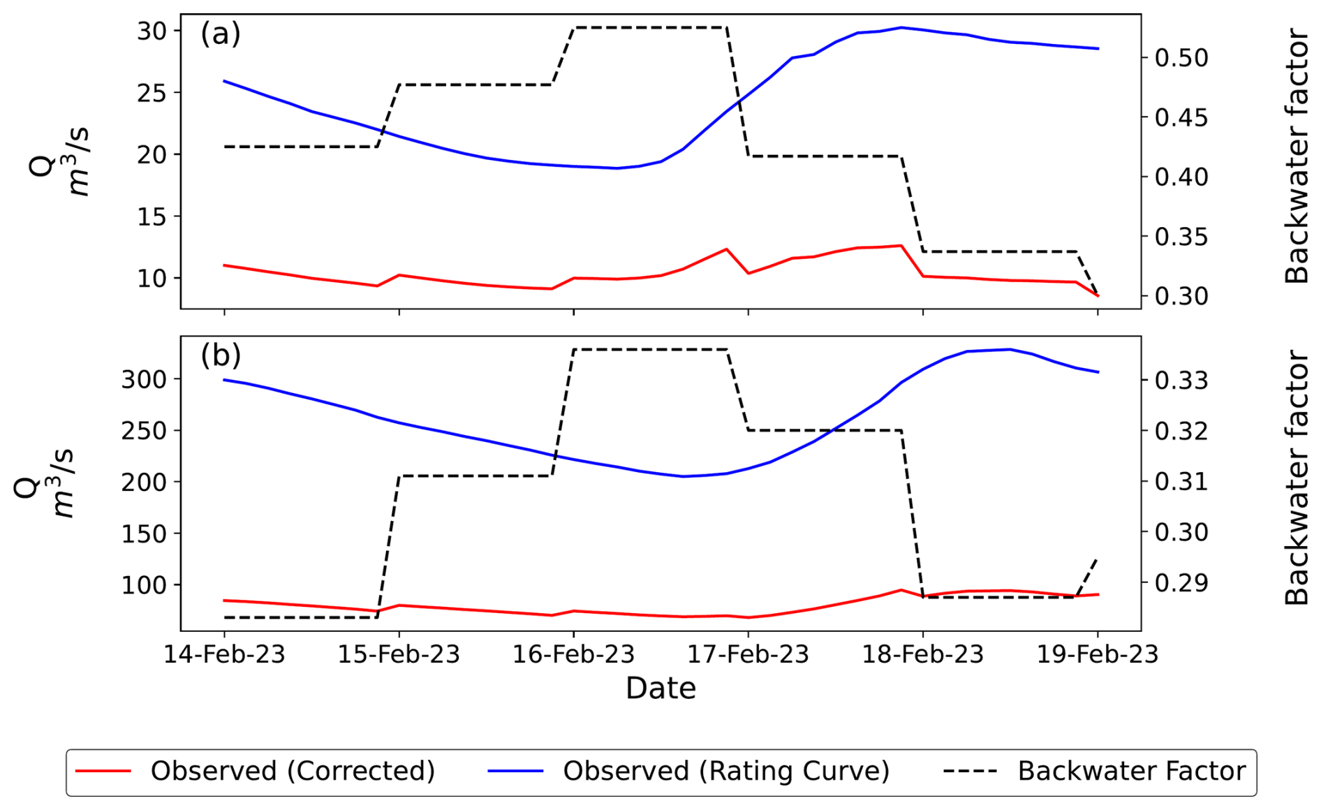
Figure 2 Example of correction of instantaneous hydrograph using daily backwater flow factors calculated by MELCCFP for Famine (a) and Saint Lambert-de-Lauzon (b) stations.

It should be noted here that the under-ice river discharge estimates produced by MELCCFP using the method discussed above are uncertain and subjective to the skill of the operator in estimating the river ice conditions.

Additional hydrometeorological data was obtained from MELCCFP for calibration and validation of the hydrological modelling framework HOOPLA (Thiboult et al., 2019). The MELCCFP provided gridded meteorological data at 0.1°-resolution grid, constructed through ordinary kriging from point observations obtained from a dense network of climatic stations across Québec (Usman et al., 2023). This data was obtained for period of 11 years from 1st January 2008 till 31st December 2018. River discharge data was also obtained for the same period and from the same source. This dataset is treated separately from the dataset in Table 2 because this dataset was not incorporated into the Delft-FEWS system as this system is not used for model calibration and validation purposes and model calibration and validation was done outside the Delft-FEWS system.

3 Methodology

The forecasting system, as first introduced by Montero et al. (2023), consists of two main modules: (i) hydrologic module and (ii) hydraulic module. The hydrologic module integrates meteorological forcing from Environment and Climate Change Canada's (ECCC) Regional Ensemble Prediction System (REPS) with the HydrOlOgical Prediction LAboratory (HOOPLA) framework (Thiboult et al., 2019) to generate ensemble based hydrological responses from the study basin. HOOPLA is a multi-model hydrological modelling framework that addresses structural uncertainty by combining different model structures. Data assimilation (DA) is implemented through the Ensemble Kalman filter (EnKf) within HOOPLA. The resulting streamflow ensemble is then post processed to extract quantile-based hydrographs (e.g. 20th, 33rd, 50th, 66th, and 80th).

The hydraulic module of the forecasting system consists of a 1D unsteady river ice hydraulic model developed in HEC-RAS (Brunner, 2016). The hydrologic and hydraulic modules are externally coupled i.e. the hydrograph from a hydrological model is applied to a hydraulic model as an upstream and/or lateral inflow boundary condition (Liu et al., 2018). This produces a unidirectional communication between the two modules. As result of this coupling a water level ensemble is generated. These simulated water levels can then be compared with the observed water level. The error magnitude guides the operator whether to accept the discharge estimates or readjust model parameters. A schematic overview of the methodology is presented in Fig. 3.

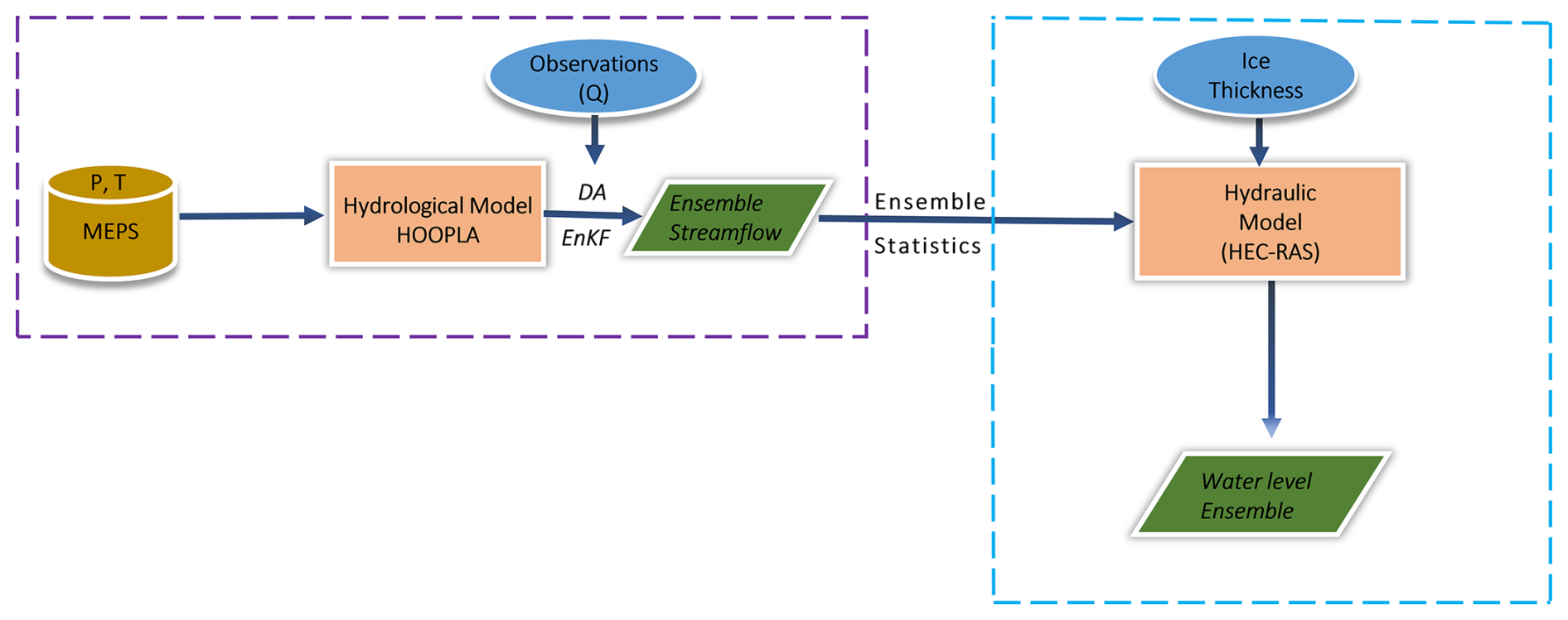
Figure 3 A schematic overview of methodology followed for probabilistic forecasting of under ice discharge. P is precipitation, T is air temperature, Q is discharge. Meteorological data is input to the hydrological modelling framework HOOPLA to produce a streamflow ensemble. Data Assimilation (DA) is implemented through the Ensemble Kalman filter (EnKf) inside HOOPLA. The streamflow ensemble is post processed for ensemble statistics and run through a river ice hydraulic model that produces a water level ensemble.

The study forms the basis for a new approach to estimate under-ice discharge through coupled modelling approach.

The different components of the forecasting system are described below.

3.1 Hydrologic Module

The hydrologic module of the forecasting system integrates a meteorological forcing source, such as the REPS system from ECCC, with a hydrological modelling framework i.e. the HOOPLA framework for producing streamflow projections. The details of these two are provided as follows:

3.1.1 Regional Ensemble Prediction System (REPS)

The Regional Ensemble Prediction System (REPS), managed by Environment and Climate Change Canada, provides a probabilistic prediction of precipitation and temperature (among many other atmospheric variables ) over a 3d forecast horizon (REPS, 2024). The REPS forecasts are generated by introducing small perturbations to the initial and boundary conditions of the model, which in return create slight variations in the prediction. This effect was described by Lorenz (1963) as the butterfly effect, where small perturbations in the initial condition are propagated in a deterministic nonlinear model and produce large variations of the states in time (Montero et al., 2023). The REPS ensemble consists of 20 perturbed members as well as an unperturbed control member. The forecasting system developed in this study integrates precipitation and temperature data imports from the REPS system. Figure 4 shows an example of the REPS prediction for precipitation on the Chaudière River for 24 January 2019 retrieved from the Canadian Surface Prediction Archive (CaSPAr) (CaSPAr, 2023).

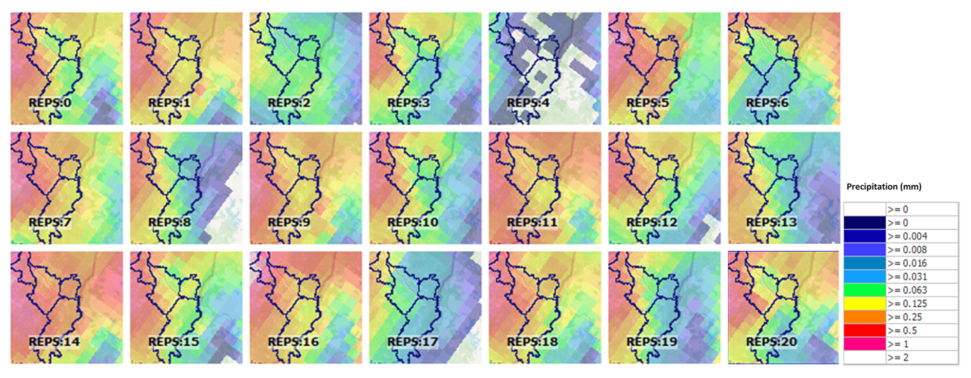
Figure 4 Members of REPS precipitation (in mm) for the 24 January 2019. Figure adapted from Montero et al. (2023).

3.1.2 HydrOlOgical Prediction LAboratory (HOOPLA)

The hydrologic module of the system is developed using the HydrOlOgical Prediction LAboratory (HOOPLA, version 1.0.1) framework, which is a multi-model hydrological modeling framework that consists of 20 conceptual lumped hydrological models, a snow accounting routine (SAR), data assimilation (DA) implemented through the Ensemble Kalman filter (EnKf), and automatic calibration algorithms (Thiboult et al., 2019). A detailed description of HOOPLA can be found in Montero et al. (2023). HOOPLA framework was calibrated and validated for the Chaudière system using the historically observed meteorological and hydrometric timeseries from 2008–2018. The models in HOOPLA were calibrated automatically through the Shuffled Complex Evolution (SCE) (Duan et al., 1992) algorithm. The algorithms are iterative and global i.e., seek optimal parameter set within the parameter space (Montero et al., 2023).

The hydrological modelling framework HOOPLA can take both deterministic and ensemble meteorological forecasts as input and produce an ensemble output. The output ensemble size depends on the size of meteorological ensemble, the number of models selected for forecast run from the framework, and the number of perturbations in the data assimilation procedure. For example, if all 20 models of the hydrological modelling framework are forced with a REPS forecast which consists of 20 meteorological members, and data assimilation is applied by perturbing 50 members, then the resulting forecast ensemble has a size of 20 000 members ($\mathrm{20}\times \mathrm{20}\times \mathrm{50}$). Processing all these members through a hydraulic model will be impractical in an operational context. Therefore, the output from each hydrological model is reduced to a single member which represents the average of the forecast ensemble for that model and thereby, leaving us with a 20-member hydrological forecast ensemble. The HOOPLA framework operates at two computational timesteps: 24 hours (24 h) and 3 hours (3 h) (Thiboult et al., 2019). For this study, a 3 h computational timestep was chosen to generate hydrological forecasts at a finer temporal resolution than the daily scale. This resolution is particularly important for capturing intraday flow variations and supporting timely flood hazard warning during mid-season or spring breakup events. Therefore, both the open water and under-ice discharges were converted to 3 h timeseries. The open water discharge timeseries was converted into 3 h timeseries by averaging the 15 min discharge data within a 3 h window. The daily under-ice discharge timeseries for the winter was downscaled to 3 h timeseries using linear interpolation i.e. each 3 h discharge value was estimated from two consecutive daily observations. This procedure used for downscaling the under-ice discharge timeseries from average daily discharge timeseries to a 3 h discharge timeseries for hydrological model calibration and validation differs from the one described in Sect. 2.2. where the backwater correction factor (estimated for the day) was applied on the uncorrected instantaneous discharge timeseries to get a fine resolution discharge timerseries. This is because the 15 min uncorrected instantaneous discharge timeseries was not available for the entire calibration and validation periods. Therefore, the procedure for obtaining a 3 h timeseries had to be adapted based on the available data.

The entire dataset was split into two equal parts following Klemeš (1986) recommendations for model calibration and validation. Data from January 2008–December 2012 was used for model calibration and from January 2014–December 2018 was used for validation. The year 2013 was used for model spin up before validation run. One of the salient features of the HOOPLA framework is that it is not data intensive and has rather simple data requirements. For calibration only precipitation, temperature, and discharge records are needed.

All 20 models included in HOOPLA framework were calibrated and validated for this study. The snow accounting routine (SAR) was implemented in the modelling framework. The SAR, referred to as Cemaneige, in the HOOPLA framework spatially distributes the catchment into five elevation bands to compute snow accumulation and melt processes (Valéry et al., 2014). The SAR is calibrated for each model individually (Thiboult et al., 2019).

3.2 Hydraulic Module

The next module in the coupled modelling system is the hydraulic module developed in HEC-RAS (version 6.0) (Brunner, 2016). This module consists of two hydraulic models: (i) a 1D unsteady river ice model to simulate simple ice cover hydraulics, and (ii) a 1D steady state river ice model to simulate ice jam profiles for the Chaudière River. The current study focuses on the estimation of under-ice discharge using the coupled modelling approach. A 1D-unsteady hydraulic model was used in this study to simulate the river ice hydraulics based on simulated/forecasted hydrographs. The model is also suitable for continuous operational applications since it can deal with dynamic flow conditions such as the ones during ice formation or ice runs (Hicks and Healy, 2003). The 1D steady state model is not used in the current study and is therefore, not described here. The modelled reach is located entirely within the Intermediate Chaudière catchment. The length of the modelled reach is 81.18 km (from chainage 106.78–25.60 km). The models have upstream boundary condition defined downstream of the Sartigan Dam and the downstream boundary condition defined at the hydrometric station at Saint Lambert-de-Lauzon (CEHQ station 023402).

The hydraulic model was adopted from the work of Ladouceur (2021) where a 1D steady state river ice model for the Intermediate Chaudière reach was developed to simulate ice jams and determine flood levels. The model geometry was constructed by merging a digital terrain model (DTM) built from LiDAR survey carried out by Ministère des Ressources naturelles et des Forêts (MRNF) and bathymetric surveys conducted by MELCCFP in 2005 and University Laval team in 2020–2021. The model geometry consisted of 481 cross-sections and includes most of the bridges within the reach. The details of these surveys can be found in Ladouceur (2021).

The steady state river ice hydraulic model by Ladouceur (2021) was modified and converted to 1D unsteady river ice model. To adapt the model for low flows more cross-sections were added through cross-section interpolation in HEC-RAS, cross-section density was especially increased near hydraulic structures and locations along the river reach where bed slope was changing. Figure 5 shows the schematic of the 1D unsteady river ice hydraulic model used in the study. The upstream boundary condition is defined as an inflow hydrograph from the Upper Chaudière, introduced downstream of the Sartigan Dam station (Station ID: 023429) at the first cross section of the model (chainage 106.78 km). A lateral inflow hydrograph, representing the flow from the Famine River (Station ID: 023422), is introduced at chainage 101.37 km. The downstream boundary condition is set as normal depth conforming to uniform flow conditions at Saint Lambert-de-Lauzon (Station ID: 023402, chainage 25.60 km).

Figure 5 Schematic of the 1D unsteady river ice Hydraulic model setup in HEC-RAS for the Intermediate Chaudière reach. The green circles represent ensemble streamflow locations obtained from the hydrological module of the system. The blue squares represent the water level control points located along the reach.

The Intermediate Chaudière catchment has several small sub-catchments. The challenge with these sub-catchments is that they are mostly ungauged. The total area of these sub-catchments is approximately 2100 km², with individual catchment sizes ranging from 20–720 km², which is considerable. Therefore, the lateral inflow contribution of these sub-catchments cannot be ignored. Bessar (2021) developed a very simple volume-based approach to derive ungauged lateral flows for the Chaudière River. This approach calculates a difference hydrograph (mathematically expressed in Eq. 1) from the routed upstream hydrographs (i.e. the hydrographs at Upper Chaudière and Famine routed through the hydraulic model) and the observed or modelled (in case of forecast) downstream hydrograph at the model outlet (i.e. Intermediate Chaudière hydrograph at Saint Lambert-de-Lauzon station). This difference hydrograph is then split into two hydrographs: a uniformly distributed lateral inflow hydrograph (Q_ULI in Eq. 2) which amounts to 60 % of the calculated difference hydrograph, and a direct lateral inflow hydrograph, representing the Bras Saint-Victor tributary (Q_BSV in Eq. 3), which is 40 % of the calculated difference hydrograph. The uniformly distributed lateral inflow hydrograph accounts for the inflow from most of the small sub-catchments while the direct lateral inflow hydrograph accounts for the Bras-Saint Victor tributary of the Chaudière River, which has an area of 720 km² and is approximately the size of Famine catchment (Fig. 5).

$$\begin{array}{}\text{(1)}& {\displaystyle }& {\displaystyle }{Q}_{\text{ungauged}}=Q_{\text{IC Observed/Modelled}}-Q_{\text{IC Routed}}\text{(2)}& {\displaystyle }& {\displaystyle }{Q}_{\text{ULI}}=\mathrm{0.60}\times Q_{\text{ungauged}}\text{(3)}& {\displaystyle }& {\displaystyle }{Q}_{\text{BSV}}=\mathrm{0.40}\times Q_{\text{ungauged}}\end{array}$$

Where Q_ungauged is the discharge from the ungauged catchments, Q_IC is the outflow hydrograph (observed or modeled) of the Intermediate Chaudière at Saint Lambert-de-Lauzon station, and Q_{IC Routed}, is the inflow hydrograph routed through entire reach. It was estimated that a 12 h delay in the application of the lateral inflow hydrographs is appropriate based on the examination of several winter hydrographs. This approach, however, introduces a new source of uncertainty in the modelling chain with regards to the application of the ungauged inflow hydrographs.

The calibration of the model using the water levels from the COBARIC hydrometric for open water conditions was done for bank full discharge conditions. This required the discharge to be in a range of 700–1000 m³ s⁻¹. The calibration showed that water level errors were within ±10 cm and the peak discharge simulated was 1002 m³ s⁻¹ observed at Saint Lambert-de-Lauzon station (Ladouceur et al., 2023). After performing open water calibration, the model was calibrated under ice cover conditions. River ice data including ice thickness and average daily flows were collected by Laval University during the winter of 2019 and 2020. This data was used for calibrating and validating the hydraulic model. Calibration was done on the data collected in 2020. The average discharge was 9.15 m³ s⁻¹ and ice thickness along the reach ranged from 0.4–1.05 m. The model showed an RMSE of 0.25 m in the calibration phase. Validation was performed on 2019 dataset, where the average daily discharge was 19.33 m³ s⁻¹ and ice thickness varied from 0.35–0.74 m along the reach. The RMSE calculated during the validation phase was 0.37. Further details on calibration and validation can be found in Ladouceur et al. (2023).

4 Delft-FEWS Platform and Testbed Development

Delft-FEWS (release 2022.02) is software platform that enables the configuration of operational forecasting systems in a flexible manner integrating existing models and available data (Werner et al., 2013). In contrast to many other forecasting systems, it contains no inherent hydrological modelling capabilities within its code base. Instead, it relies entirely on the integration of external (third party) modelling components (Montero et al., 2023). Delft-FEWS is extensively used in Canada by different local and government agencies, among them are: Alberta's River Forecasting Centre, the Water Security Agency in Saskatchewan, the MELCCFP of Québec, New Brunswick's River Forecast Centre, the territorial governments in the Yukon and Northwest Territories, along with key utility providers such as BC Hydro, Manitoba Hydro, and Ontario Power Generation (Arnal et al., 2023; Montero et al., 2023).

The Delft-FEWS platform can be considered as a model-agnostic platform (Arnal et al., 2023), which takes care of preparing the data that each individual model requires to produce a simulation. This is done through the concept of a “General Adapter”, which is a processing module in Delft-FEWS that allows to connect the data to the model by three basic components: (i) exporting data from the system to specific directories as published interface-extensible markup language (pi-xml) or NetCDF files, (ii) executing activities, and (iii) importing data back into the system from pi-xml or NetCDF files.

Delft-FEWS follows a data-centric approach as all modules are connected to a central database (Gijsbers et al., 2008). This design ensures consistent access to data across all users, supports real-time forecasting, visualization, and decision support, and provides the flexibility to configure applications tailored to the needs of individual forecasting centres.

4.1 River Ice Forecasting Testbed (RIFT) for the Chaudière River

The River Ice Forecasting Testbed (RIFT) for the Chaudière River was configured in the Delft-FEWS platform, and it enables the integration of: (i) observed and prognostic meteorological variables, (ii) hydrological modelling toolbox, (iii) hydraulic model component, as well as components that enable (iv) real-time modification of model parameter and data processing. Figure 6 illustrates the process of the forecast workflow and the main variables that are involved in each step of the forecast (Montero et al., 2023).

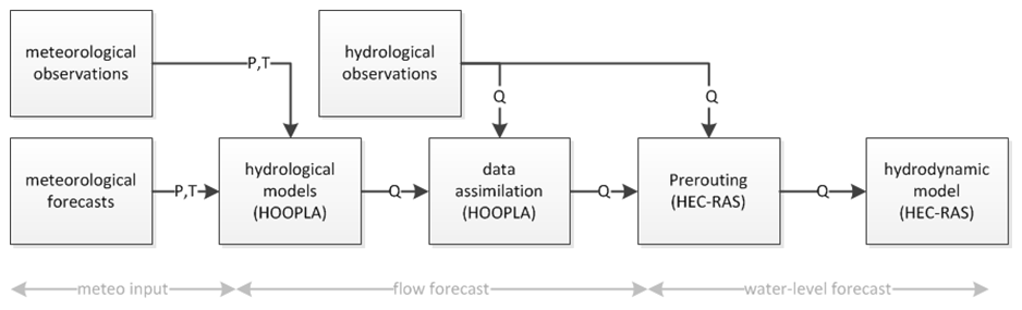
Figure 6 Schematic overview of workflow for the hydrological forecasts. P is precipitation, T is air temperature, Q is discharge. Figure adapted from Montero et al. (2023).

The workflow manages the meteorological and hydrological observations, as well as the meteorological forecasts. The observations are pre-processed in the platform to calculate basin average values using Kriging interpolation that are required by the hydrological toolbox (HOOPLA) to simulate the discharge data to be used in the hydrodynamic model (Montero et al., 2023). Finally, the hydrodynamic model is compared to observations to adjust any parameters or variables within the workflow (Fig. 6). Note that HOOPLA assimilates the hydrological observations to produce updated model states to improve the hydrological simulation. The system is configured to produce a pre-routing step that allows to create simulated hydrological inflows to the unsteady hydrodynamic model of the Hydraulic Module.

The processing diagram to create the basin average variables is illustrated in Fig. 7 (Montero et al., 2023). The processing for precipitation is done by merging together individual station observations to create a spatially distributed precipitation grid over the catchment through the Kriging interpolation procedure. The spatially distributed precipitation can then be averaged within each basin (Montero et al., 2023). The same procedure is performed for the observed temperature variable, with an additional step of estimating the temperature of each station at sea level. After which the Kriging interpolation and the subsequent basin averaging procedures are performed (Montero et al., 2023).

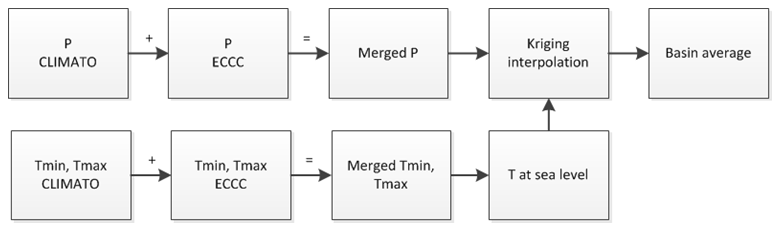
Figure 7 Preprocessing of observed data to create inputs for hydrological historical update runs. P is precipitation and T is air temperature. Figure adopted from Montero et al. (2023).

From an operational perspective, it is desirable to be able to interact with the models and to be able to modify sensitive parameters in a convenient manner. This flexibility in Delft-FEWS is provided by Modifiers. The current system for the Chaudière River is configured to have three modifiers' groups (Montero et al., 2023). The first modifier corresponds to the modification of the parameters used as a proxy of the hydrological routing to compute the ungauged inflows between Sartigan and Saint Lambert-de-Lauzon stations (Montero et al., 2023). The parameters corresponding to this first group of modifiers are the shift in the hydrograph (i.e. the time lag in the application of the difference hydrograph) and the split factor i.e. the ratio in which the difference hydrograph should be divided into to estimate the uniform and direct lateral inflow as described in Sect. 3.2. By default, the hydrograph shift is kept to 7 h in the Delft-FEWS configuration whereas for the distribution of the difference hydrograph (i.e. Q_ungauged in Eq. 1) the ratio is set as 60:40 between the uniformly distributed lateral inflow and the direct lateral inflow.

The second modifier group allows the operator to modify the ice cover in the HEC-RAS model (Montero et al., 2023). These modifications correspond to ice thickness and under-ice roughness. Following the river ice characterization described in Ghobrial et al. (2023), the model was split into 9 reaches (subject to alteration). The ice conditions were considered homogenous within each reach. The modifier has these pre-defined reaches, where the ice thickness and ice roughness can be changed both for the main channel as well as for the banks (Montero et al., 2023).

The third modifier group allows the operator to directly modify the inflow hydrographs (through operations such as multiply, divide, add or subtract by certain factor) that are linked to the boundary conditions of the hydraulic model, i.e., the hydrographs at Sartigan, Famine, Saint Lambert-de-Lauzon, as well as the hydrographs at Bras-Saint-Victor and the uniformly distributed flow (Montero et al., 2023).

Figure 8 shows the configured user interface of the River Ice Forecasting Testbed (RIFT) for the Chaudière River. Note that the platform provides diverse information regarding spatial distribution of meteorological variables (as seen in Spatial Data Display), the visualization of real-time scalar information showing observed and simulated time series at specific gauging stations (through the Hydrological Module Display), as well as the three possible modifiers to introduce operational decisions to the forecast workflow (via Modifiers Configuration). The platform is intended to facilitate the complex dynamics of river ice modelling by updating hydrological and hydraulic components and a quick verification with observed time series imported into the system. The complete forecast workflow is summarized in the Forecast Tree, where a series of nodes trigger individual components of the workflow such as the meteorological data imports, hydrologic simulations, and the hydraulic simulations, both for the update and the forecast runs.

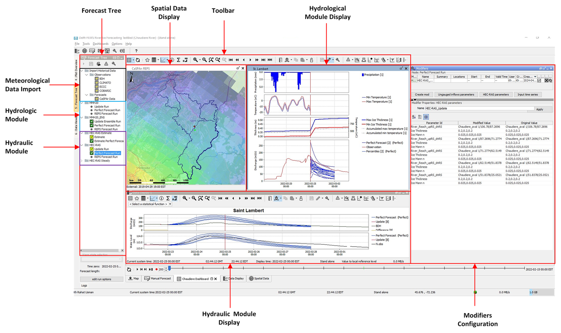
Figure 8 A screenshot of the Delft-FEWS River Ice Forecasting testbed system for the Chaudière River.

The system has been developed for operational forecasting of under-ice river discharge in a probabilistic manner. The probabilistic approach helps address various sources of uncertainty in the modelling chain such as meteorological forcings uncertainty; hydrological model structure uncertainty; model states uncertainty; and parametric uncertainty, as well as captures variability and presents a range of future scenarios to the decision makers who can then make better informed decision.

However, an important aspect of an operational forecasting system is the computation time. Ensemble based methods are usually computationally expensive and time consuming. For example, with a 2.90 GHz 8-Core(s) processor and 16 GB of RAM, a single forecast run for HOOPLA, consisting of only one meteorological member for the three catchments takes approximately 2 min and a single member unsteady run in HEC-RAS takes approximately 4 min. From this we can estimate that a 20-member ensemble run for a single forecast in HEC-RAS will take approximately one hour for a 5 d long forecast. This can be solved in Delft-FEWS by splitting the workflow into multiple computational nodes that run in parallel, if necessary.

Both the Hydrological and Hydraulic modules are configured to have an “Update Run” component in addition to the “Forecast Run” component. The function of the Update Run component in both these modules is to produce updated model states for a Forecast Run. The Update Run feeds on available observed data prior to the forecast issue time (i.e. T₀). The simulation performed by the models in this run create a new set of model states (i.e. updating storages in hydrological models, and water levels in the hydraulic model) that best describe the catchment conditions. In case of the hydrologic module, data assimilation is implemented in the Update Run component through the Ensemble Kalman Filter (EnKF).

The hydrological forecast ensemble is post-processed to calculate ensemble statistics (i.e. percentiles). The 20th, 33rd, 50th, 66th, and 80th percentiles of the resulting ensemble are calculated. These five members are passed over to the hydraulic module to simulate water levels.

4.2 RIFT Operating Procedure

A single streamflow and water level hindcasting event is described in detail, to explain the everyday operational procedure of the system for forecasts issued on three consecutive days from 23–25 February 2022. MELCCFP carried out discharge measurement at the Intermediate Chaudière hydrometric station (Station: 023402) on 23 February 2022. The measured discharge at this location averaged for the day was reported to be 138.30 m³ s⁻¹. The ice thickness measured by the Laval University team on 22 February 2022, at Chaudière on average was 0.5 m. For the Upper Chaudière and Famine sub-catchments corrected winter discharge is considered since measured discharge is not available on the same day.

Meteorological observations (MELCCFP, 2022) were used as forcing data (Perfect Forecast) to keep the forcing uncertainty low. Figure 9 shows the meteorological conditions observed over the Upper Chaudière catchment during the forecasted period. Meteorological conditions over the other two catchments i.e. Famine and Intermediate Chaudière were similar to the Upper Chaudière. The accumulated precipitation between 23 February–2 March 2022, was recorded to be 22.1 mm for the Upper Chaudière, 18.9 mm for the Famine watershed and 20.3 mm for the Intermediate Chaudière. The temperatures during this period mostly remained below freezing indicating that most of the precipitation received was solid precipitation (i.e. snow). However, positive temperatures were recorded for the three sub-basins on 23 February 2022; the precipitation data shows a rainfall event making the conditions suitable for runoff generation.

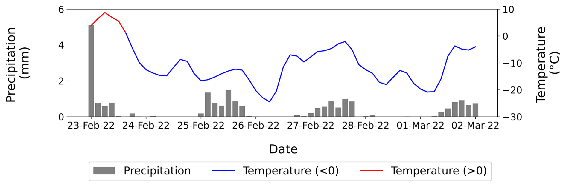
Figure 9 Meteorological conditions observed over Upper Chaudière during the forecasted event. The average temperatures during the forecast period remained below freezing. Similar conditions were observed at the other two catchments.

The hydrologic module of the couple modelling system was updated for the hydrologic states by running it in a batch simulation mode from 15 November 2021, till 23 February 2022, at a daily interval (this is not to be confused with computation time step of the hydrological modelling framework which is 3 h). This means that for a duration of 100 d, the hydrological model states were updated every day through continuous simulations and data assimilation. This sets up the model states in optimal conditions for forecasting. Perfect Forecasts for 23–25 February were run (each forecast run is followed by an update run to set up the hydrologic states for the next forecast run). After the hydrologic module has finished running, the hydraulic module of the system is executed in a similar manner. The hydraulic module is first run in update mode where the input data consists of observed flows. This run updates the states parameters of the hydraulic module based on observations. This allows the operator to make a visual comparison between the simulated an observed stage at T₀ (T₀ is the time at which the forecast is to be made) and update/modify any required model parameter such as ice thickness or under ice roughness. The next step is to run the hydraulic module in forecast mode where the input data is now passed from the hydrologic module consisting of the forecasted streamflow ensemble.

4.3 Testing and Evaluation

For the current study, the system was tested by hindcasting events for which manual discharge and ice thickness measurements were available. This is important since the inherent uncertainty within the winter records is significantly large. Moreover, to reduce the element of meteorological uncertainty in the hindcasted events, the observed meteorological data was used as forcing data which is termed as “Perfect Forecast.” For this study, the hindcasted events are summarized in Table 3. For each of these events, the forecast horizon is set as 5 d for both the hydrological and hydraulic module. However, it should be noted that the manually measured discharge is available only for one day within the forecast horizon and for the remaining length of the forecasted period the backwater corrected discharges were used for comparison between observed and simulated flows. Also, the measured discharges for the Intermediate Chaudière (measured at Saint Lambert-de-Lauzon gauging station) are used, whereas for the Upper Chaudière and Famine sub-catchments backwater corrected discharges are used for comparison with simulations. This is done with two main considerations: (i) Intermediate Chaudière is significant for lateral inflow estimation, and (ii) Intermediate Chaudière hydrometric station also produces stage data which is used in the evaluation of the hydraulic module of the system, hence, accurate discharge information at this location is critical for performance evaluation of the system.

Table 3 Summary of the Events used to evaluate the system.

For the first event (Table 3) detailed ice thickness measurements along the modelled reach were available from Ghobrial et al. (2023) and were used in the model. For the remaining events a measured ice thickness at key location along the river was used. The performance of the hydrologic module is evaluated at all three control stations i.e. the hydrometric stations. While for the hydraulic module the performance is evaluated at two water levels stations which are Sainte Marie and Saint Lambert-de-Lauzon. There are two reasons behind excluding the rest of the COBARIC stations. First is the reliability of stage data which is the case at Beauceville where the station is location under a bridge and immediately downstream of an island, thus the ice conditions at this location are affecting the local stage in an unexpected manner which cannot be accounted for in a simple hydraulic model (Ladouceur, 2021). Second, the sensor at some gauging stations is not installed at the thalweg of the river and thus cannot measure water levels below a specific threshold. This is the case for the Valee Junction station where there is a threshold elevation of 142.96 m, below which the station cannot produce water level records.

The preliminary evaluation of the system is conducted by computing root mean square error (RMSE) and percent bias (PBias) as deterministic scores. RMSE is a commonly used metric which is a measure of average magnitude of error between model predictions and observations. A lower value of RMSE is an indicator of good model performance. However, this metric is absolute metric and does not indicate the direction of error i.e. either the model is overestimating or underestimating. For determining the direction of error, the second metric which is the percent bias (PBias) is used. PBias is a metric that determines the error in model prediction relative to the observations and indicates the direction of error i.e. positive error (overestimation) or negative error (underestimation). A value of PBias close to zero is desirable to have an unbiased modelling system. The deterministic metric is calculated from the average ensemble values for each event (Anctil and Ramos, 2017). For RMSE, the squared error for each ensemble member at each time step was calculated and then the root mean square was calculated to get the RMSE of the ensemble at each time step. Similarly, PBias for each ensemble member was calculated at each time step and then these individual PBias values were averaged to calculate the average PBias of the ensemble. The overall performance of the system is expressed as an average of the metrices over the three simulated events. Since the current dataset comprised of only 3 measured events, each measurement was placed at 4–5 successive forecast days to evaluate the performance metrices. This gives a total of 14 evaluation points against the three measurements. The ice thicknesses are assumed to remain constant during the forecasted periods for each event. Bootstrapping was applied to calculate the 95 % confidence intervals for the deterministic scores for a detailed description of uncertainty in the system's performance (Velázquez et al., 2010; Bessar, 2021).

5 Results and Discussion

The results section is structured to first present results for the calibration and validation of the hydrological modelling framework HOOPLA, followed by results from the evaluation of RIFT.

5.1 Calibration and Validation of HOOPLA

HOOPLA framework calibration and validation results are presented in Fig. 10 for the three study catchments over a 10 yr long observed timeseries. Both calibration and validation periods show good agreement with the observations for all three catchments.

Figure 10 Calibration and validation of HOOPLA framework performed on the three sub-catchments defined in the Chaudière River Basin. (a) shows the results for the Intermediate Chaudière sub-catchment, (b) shows the results for the Famine sub-catchment, and (c) shows the results for the Upper Chaudière sub-catchment.

The modified Kling–Gupta efficiency (KGEm) was computed (Kling et al., 2012) as the calibration objective function and same metric was used for evaluating model performance during the validation period. Figure 11 presents the distribution of the calculated KGEm for each catchment during model calibration and validation periods. The framework shows very high performance for all three catchments during the calibration period with no outliers and KGEm consistently above 0.88 (KGEm ranges between −∞ to 1, with 1 being perfect fit). During the validation period the Intermediate Chaudière catchment showed nearly similar performance to its calibration with KGEm ranging between 0.89–0.93 for all the models. In the case of Famine catchment, the HOOPLA framework performance during validation was slightly superior to the calibration period with KGEm values ranging between 0.89–0.92 for most of the models except for one outlier, Model 8, which had a KGEm value of 0.83. In the case of Upper Chaudière catchment, the performance during validation was inferior to calibration, for this catchment the performance metric remained in a range of 0.84–0.90 during the validation period which is still considered as very good performance by the framework. The analysis of the KGEm metric revealed that during validation period the models overestimated flows in the catchment resulting in a higher positive bias. Moreover, the models didn't capture flow variability as well as they did during the calibration period. This led to a slightly reduced performance during the validation period.

Figure 11 Boxplot showing the modified Kling-Gupta Efficiency (KGEm) distribution of all 20 hydrological models in HOOPLA framework for each catchment during calibration and validation periods.

5.2 Hindcast 23–25 February 2022

Figure 12 presents the hydrological forecast for the three modelled catchments. Compared to the corrected observations produced by MELCC, the forecast issued on 23 February 2022, shows that the models overestimated the streamflow flow for the Upper Chaudière sub-catchment. For Famine the observed hydrograph falls within the ensemble for the first few timesteps (8 timesteps) and later the models tend to underestimate the discharge. For the Intermediate Chaudière there is overestimation in the peak discharge, but the hydrograph recession mostly falls within the ensemble bounds.

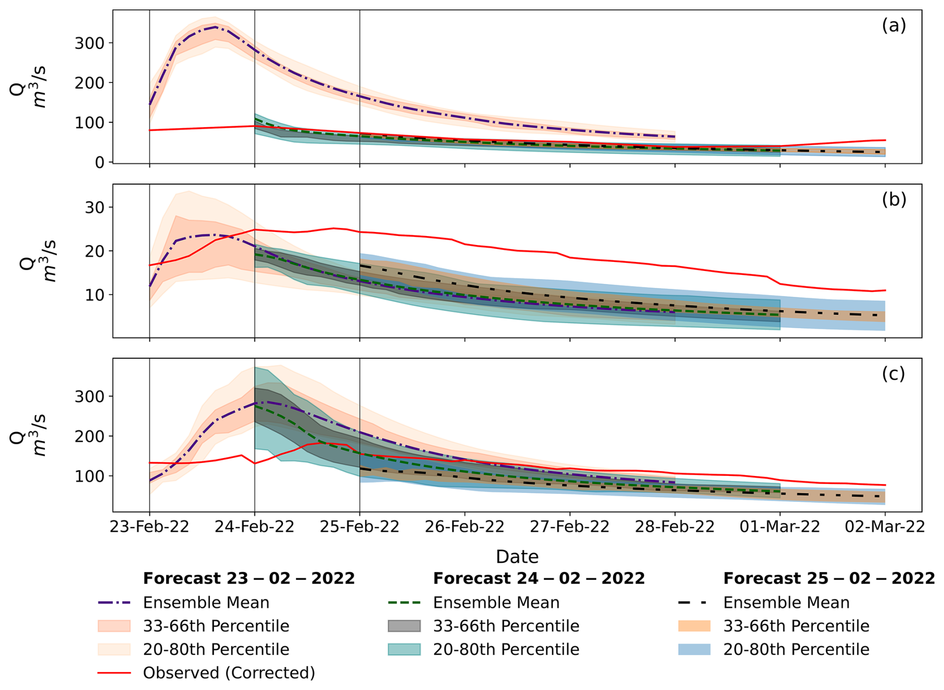
Figure 12 Ensemble hydrologic forecast evolution for 23–25 February 2022 at the three sub-catchments of the Chaudière River. The grey vertical lines in the subplots correspond to the issue time of each forecast. The subplots (a–c) show the hydrological forecasts at Upper Chaudière, Famine and Intermediate Chaudière respectively.

Subsequently, hydrological forecasts are issued on 24 and 25 February 2022. For the Upper Chaudière, the gap between the observed and forecasted hydrograph is now reduced and in fact the observations fall within the ensemble bounds (the ensemble is quite narrow in this case) until the March 01, 2022, after which the models underestimate the flow. For Famine, the forecasted hydrograph is an underestimated one.

The impact of data assimilation and model states update is visible for the subsequent forecasts. The discharge at the forecast issue time (i.e. 24 and 25 February respectively) is higher than the previously forecasted values however, it is still not high enough to match the observations. In the case of Intermediate Chaudière, the error at forecast issue time is high but starts reducing over time, as the forecast horizon is reached the forecasted hydrograph dips below the observed one and the observations no longer fall within the ensemble bounds.

Figure 13 presents the results from the hydraulic module of the system. For the water level forecast issued on 23 February 2022, the observed water levels at Sainte Marie fall within the ensemble for the first four days of the forecast period and on the fifth day the observed levels are higher than the simulated ones. The ensemble mean remain higher than the observed levels for the first three days and later dips below the observed levels. The result at Saint Lambert-de-Lauzon station for the forecast on 23 February is similar to Sainte Marie, however the difference is that the ensemble mean and observed water levels are superimposed indicating a very small error between modelled and observed levels for the first three days but later the forecast ensemble dipped below the observations. For the subsequent forecasts i.e., forecasts issued on 24 and 25 February the error in water levels is higher. Montero et al. (2023) have demonstrated the sensitivity of water levels to discharge. The fact that the simulated water levels matched the magnitude and shape of the observed water levels (Fig. 13) improves confidence in the simulation and indicates that the system is performing very well when using the simulated inflow hydrographs from HOOPLA as input to the HEC-RAS model. The fact that these inflow hydrographs were much higher than the discharges reported by MELCCFP (Fig. 12) indicate that the reported under ice discharges may not be accurate and the uncertainty with regards to the estimation of backwater factor used to produce these discharges is very high.

Figure 13 Ensemble water level forecast at Sainte Marie (a) and Saint Lambert-du-Lauzon (b) stations along the Chaudière River for forecasting on 23–25 February 2022. The grey vertical lines in the subplots correspond to the issue time of each forecast.

The measurement done by MELCCFP on 23 February 2022 is a point measurement, the intraday discharge variability cannot be established from a point measurement, furthermore, the discharge estimates produced are reported as an average for the entire day hence the intraday variability is lost. Hydrological modelling produces discharge estimates at a finer resolution (i.e. 3 h resolution) and the water level records, which are available at an even finer resolution (i.e. 1 min resolution), can be used to confirm streamflow projections through hydraulic modelling.

5.3 System Performance

The performance metrics evaluated for the system are presented in Fig. 14. The top panels (subplots a and b) represent the results for the hydrologic module and the bottom panels (subplots c and d) represent the results for the hydraulic module. The metrics are evaluated over the forecast lead times. Since the system ran in “Perfect Forecast” mode, the meteorological uncertainty is low.

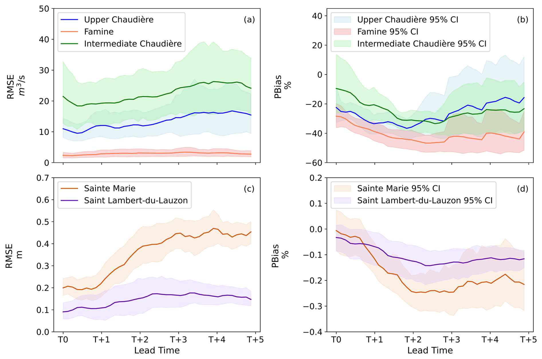
Figure 14 Performance evaluation of the coupled modelling system using RMSE and PBias scores. The top panel (a, b) represents the results of hydrologic module, while the bottom panel (c, d) represents the results of hydraulic module.

The RMSE evaluation of the hydrologic module presented in Fig. 14a shows that its performance remains nearly consistent over the forecast horizon with gradual increase in the errors over the lead times. For Upper Chaudière, the RMSE is in a range of 9.5–16.8 m³ s⁻¹. The 95 % confidence interval calculated through the bootstrap method shows that the forecast uncertainty is smaller at T+0 and as the forecast window moves in time the forecast uncertainty gradually increase. Beyond T+3, the forecast uncertainty has reached its peak and remains stable till the end of the forecast period. Average daily discharge during the winter period was calculated over a period of seven winters between 2017–2023 for each catchment. A comparison of the RMSE at Upper Chaudière with the average winter discharge of 85.5 m³ s⁻¹ shows that the RMSE is well below the historical average. Famine also shows a trend similar to Upper Chaudière, where its RMSE increases gradually over the forecast period from 2.8–3.4 m³ s⁻¹. The 95 % confidence interval for Famine grow wider beyond T+3 indicating higher uncertainty in the forecasted discharge. The comparison of RMSE with average daily flow of 20 m³ s⁻¹ shows that the errors are small. In case of Intermediate Chaudière, the RMSE ranges from 18.4 m³ s⁻¹–26.3 m³ s⁻¹ over the forecast window. The trend of uncertainty in this catchment is also similar to Famine and Upper Chaudière. However, the confidence intervals are wide from the beginning of the forecast representing higher uncertainty which further grows over time reaching its peak beyond T+3 (similar to the other two catchments). The RMSE is much smaller than the average daily flow at Intermediate Chaudière which is estimated to be 165.5 m³ s⁻¹.

The PBias analysis for the hydrologic module is presented in Fig. 14b. This analysis shows that the forecasted discharges were underestimated in all three catchments. The Upper Chaudière discharge is initially underestimated by 22 % and the underestimation continues till T+2 reaching a maximum value of 36 %. Beyond T+2 the bias starts reducing consistently until the end of the forecast window reaching its lowest value of 15 % underestimation. The confidence interval is narrow up until T+2 indicating consistent performance however, it widens significantly beyond this point till the end of the forecast window indicating higher uncertainty in the forecast. For Famine, the initial underestimation is by 28 % and as the forecast progresses in time the underestimation keeps on increasing reaching nearly 47 % underestimation. The confidence interval is narrow at the beginning of the forecast period. The forecast uncertainty increases rather sharply at T+3 and remains stable. In the case of Intermediate Chaudière, the initial underestimation is discharge is around 10 % but this gradually increases over time reaching a peak underestimation of 33 % between T+2 and T+3. The confidence interval increases beyond this point indicating higher uncertainty in the forecast. In case of Intermediate Chaudière, the forecast uncertainty is higher at the beginning of the forecast as well showing a similar trend to its RMSE evaluations.

The hydraulic module is also evaluated with the same metrics. RMSE, calculated for Sainte Marie and Saint Lambert-du-Lauzon water level stations, is presented in Fig. 14c. At the Sainte Marie station the RMSE is in a range of 19–46 cm. The RMSE at this station increases sharply after T+1 and then remains stable after T+3. The confidence interval is also wide indicating high water level uncertainty at this station. The Saint Lambert-du-Lauzon station, however, shows stable performance. The RMSE at the station is in a range of 9–17 cm and it increases gradually over time. The confidence interval is wider between T+1 and T+3 indicating relatively higher uncertainty in the middle of the forecast window at this station.

The PBias analysis presented in Fig. 14d shows that the water levels are underestimated which is consistent with the hydrological analysis i.e. underestimated discharges will produce underestimated water levels. At Sainte Marie station the water levels are underestimated in a range of 0.01 %–0.25 %. The uncertainty in the water level estimates increases beyond forecast lead time T+2. In case of Saint Lambert-du-Lauzon the water level underestimation ranges between 0.03 % to 0.14 %. The underestimation increases gradually over time. The uncertainty in the water levels follows the same trend as in case of water level RMSE at this station.

The current analysis of the coupled modelling system is done with a limited dataset which renders it sensitive to extreme events. The analysis for the hydrologic module shows higher deviations from the observations as quantified through the PBias metric especially, for the Famine sub-catchment. The uncertainty quantification done through bootstrap confidence intervals showed that uncertainty tends to increase as we move further along the forecast horizon. This can be attributed to the uncertainty in the model states since meteorological uncertainty is minimal due to “Perfect Forecast.” Furthermore, apart from a few observations (i.e. the manually measured discharges) in the dataset the uncertainty associated with the remaining observations is unknown. The hydraulic module on the other hands showed a satisfactory performance. The PBias and RMSE values are within narrow and acceptable range. The RMSE at Sainte Marie was relatively high as compared to Saint Lambert-du-Lauzon station. A reason for this could be the local river ice conditions at the station. The ice thickness, which has a major influence on water level, at this station was assumed to be equal to the downstream ice cover measured at Saint Lambert-du-Lauzon. This, in addition to underestimation in discharge, is likely to induce more errors and uncertainty at this station.

At Intermediate Chaudière, the PBias analysis of the hydrologic and hydraulic module shows underestimation. This indicates that the hydrologic projections need to be adjusted before being fed to the hydraulic module. The magnitude of underestimation of hydrologic projections is however uncertain due to the uncertainty of under-ice discharge observations. These observations are highly subjective and dependent on the skill and experience of the technician producing them. According to the study by Dahl et al. (2019) the error in the produced timeseries can be as high as 156 %. For the current discharge dataset, an estimate of uncertainty is not available, so it is extremely difficult to know the true error in the hydrologic module projections. The smaller error in the hydraulic module does indicate that the hydrologic projections might not be significantly off. This is the benefit that can be harvested from the coupled modelling approach as implemented in this study for estimating under-ice discharge.

The coupled modelling approach can surely benefit from a few extensive under-ice discharge measurement campaigns that can provide critical data for hydrological model calibration as well as model evaluation. The approach can be transferred to catchments suffering from river ice conditions with an appropriate hydrological modelling framework that best describes the catchment hydrology and a hydraulic model setup for a reach with water level and ice thickness measurements available.

The main limitations for the current study include uncertainty in the observed discharge (i.e. the corrected discharge timeseries) used for data assimilation and performance evaluation, and unavailability of detailed ice cover data along the river. These limitations impact our ability to accurately evaluate the model performance and undertake efforts to improve hydrologic projections during the ice-covered period. Another limitation for the current modelling setup is with the hydraulic model that become unstable when the discharge in the channel is below 15 m³ s⁻¹.

6 Conclusions

In this study we demonstrate the development and capabilities of a coupled (hydrologic and hydraulic) modelling system for operational forecasting under river ice conditions and assess the system's functionalities over selected winter events. The system is developed for the Chaudière River in Québec, Canada. The hydrologic modelling framework HOOPLA was coupled with a 1D unsteady river ice hydraulic model in HEC-RAS. The operational forecasting system was configured in Delft-FEWS, which provides a flexible environment for data management and model integration.

The current study conducted a preliminary analysis of the developed system based on handful events where in-situ data was available. The under-ice river discharge data retrieved from observations is highly uncertain since there is no reliable method available to date for its estimation other than direct measurements, which are usually sparse given challenging conditions. An additional challenge with this data is its resolution. Winter records are usually produced at a daily resolution which fails to account for the intraday variability, although it can be argued that the winter period is usually stable with not much flow variability within a day however, considering the dynamic nature of river ice processes, especially during the breakup period, a finer resolution of under ice discharge is of value. The chosen events were simulated using meteorological observations as forcing data (i.e. Perfect Forecast) and were analyzed using deterministic scores namely RMSE and PBias. The hydrologic module of the system under-estimated winter flows for the modelled catchments. Despite the RMSE values being low, the simulations showed significant deviations from the observed (corrected rating curve discharge) (i.e. PBias metric).

The hydraulic module showed better performance with the RMSE staying within an acceptable range in the initial forecast lead times. The water level forecast generally remained under-estimated as evident from the PBias analysis, but it was within an accepted margin. This analysis though needs to be interpreted with caution since it is based on limited data and warrants further investigation using a larger dataset to improve confidence on the system.

The coupled modelling approach is gaining popularity in river-ice modelling especially in the domain of ice jam flood assessments and forecasting (Chen and She, 2023; Lindenschmidt et al., 2021, 2019). However, this has not been applied to continuous estimation of the under-ice discharge. The study by Chen and She (2023) applied Soil and Water Assessment Tool (SWAT) coupled with River 1D model for the Peace River Basin to study the influence of streamflow from ungauged sub-catchments on peak flow under both open water and river ice breakup conditions and found discrepancies in streamflow simulations during the river ice conditions and associated them to the uncertainties in Snow Water Equivalent (SWE) and emphasized on the need for improvements in hydrological modelling of under-ice discharge. Lindenschmidt et al. (2019) coupled the MESH (Pietroniro et al., 2007) hydrological model with RIVICE (Canada, 2013) process based river ice model for probabilistic operational real-time ice jam flood forecasting. The study showed value in utilizing the coupled hydrologic and hydraulic modelling for river ice forecasting applications. The current study takes a simplistic approach in hydraulic modelling as compared to these studies by avoiding river ice process modelling and focusing on rive ice hydraulics under fully developed ice cover conditions. As the aim to the improve the method for under-ice discharge estimation and forecasting.

The current study lays foundations for a modelling system that can be applied for reliable estimation and forecasting of winter flows. The coupled modelling approach has demonstrated potential in resolving the long-standing challenge in the estimation and forecasting of under-ice river discharge. This approach provides a comprehensive method to the forecasting agencies in cold climate region to manage water resources throughout the year and reduces the element of subjectivity in the under-ice discharge estimates. It also provides a mechanism to make use of all available hydrometeorological variables such as precipitation, temperature, streamflow, and water level information to estimate under-ice flows at desired temporal resolution. The ensemble-based approach caters for the uncertainty arising from various sources in the modelling chain and presents a complete picture of the future events. However, this approach requires further testing and evaluation through reliable winter gauging dataset that can be used in model calibration as well as performance evaluation.

In the future, the team is focussed on increasing the event dataset to further test and optimise the system. Special focus will be dedicated to addressing the identified limitations in the current modelling setup to improve forecasting results and reduce modelling uncertainties. It also focuses on the assessment of the steady state hydrodynamic simulation configured within the hydraulic modules of the system.