The Met Office Unified Model Global Atmosphere 8.0 and JULES Global Land 9.0 configurations

We describe Global Atmosphere 8.0 and Global Land 9.0 (GA8GL9) that are science configurations of the Met Office Unified Model and Joint UK Land Environment Simulator (JULES) land surface model developed for use across weather and climate timescales. GA8GL9 builds upon GA7GL7. It not only consolidates the changes made for the climate branch configuration GA7.1GL7.1 (the atmosphere and land components of the physical model used in HadGEM3-GC3.1, UKESM1 and UKESM1.1 which were all used in the Met Office's CMIP6 submissions) and NWP branch configuration GA7.2GL8.1 (the operational global NWP model at the Met Office between 2019 and 2022), but also includes developments to most areas of the science. Some of the key changes include: prognostic-based entrainment, which adds convective memory and improves precipitation rates and spatial structures; time-smoothed convective increments, which improves the convection-dynamics coupling and greatly reduces the detrimental dynamical effects of convective intermittency; a new riming parametrisation, which increases the amount of supercooled water and hence reduces Southern Ocean biases; and a package of land surface changes, which improves the forecast of near-surface fields and hence removes the need for the aggregate surface tile in NWP applications. Several changes are made that reduce numerical artefacts and improve the numerical stability of the model. The NWP and climate performance of GA8GL9 is evaluated against the previous configuration, GA7GL7. In NWP tests GA8GL9 is shown have reduced errors and improved spatial structure. The mean climate in GA8GL9 is shown to be improved relative to GA7GL7 with notable improvements in the top of atmosphere outgoing shortwave radiation. GA8GL9 is the atmosphere and land component of GC4, and GC4 has been used as the operational global NWP model at the Met Office since May 2022.

1 Introduction

At the Met Office and other UM partners the Unified Model (UM) and the Joint UK Land Environment Simulator (JULES) are used in defined Global Atmosphere (GA) and Global Land¹ (GL) configurations to simulate the global atmosphere-land system. The GA/GL development process is described in Walters et al. (2011). Each subsequent GA configuration is built upon the previous configuration. For example, the subject of this report, GA8GL9, is built upon the previous configuration GA7.0GL7.0 (Walters et al., 2019). Each GA/GL configuration is designed for use across all timescales and global resolutions and hence is assessed in terms of both its climate and Numerical Weather Prediction (NWP) performance. Global coupled (GC) configurations also include Global Ocean (GO) and Global Sea-Ice (GSI) components to simulate the global atmosphere-land-ocean-sea-ice system.

Branch configurations may be developed from the GC/GA/GL trunks for use in specific applications. These will usually include a small number of tunings and science developments pulled forward from the next development cycle. GA7.0 spawned two branch configurations: GA7.1 (Walters et al., 2019), which was intended for climate applications, and GA7.2 (Willett et al., 2023), which was intended for NWP applications. Note that GA7.2 is developed from GA7.0 and not from GA7.1. GA7.1 is the atmospheric component of the physical model used in HadGEM3-GC3.1 (Williams et al., 2017), UKESM1 (Sellar et al., 2019) and UKESM1.1 (Mulcahy et al., 2023), which were all used in the Met Office's CMIP6 submissions. GA7.2 was the operational global NWP atmosphere model between December 2019 and May 2022. GA8 reintegrates the changes made for both GA7.1 and GA7.2 back onto the GA trunk. For brevity in this document the suffix “.0” will be dropped when referring to the trunk configurations (GA7.0, GL7.0, GA8.0, GL8.0, GL9.0).

The land component described in this paper is GL9 rather than GL8 because an intermediate land configuration, GL8 (Willett et al., 2023), was defined in 2018. GL8 includes improvements to sea-ice drag and the representation of snow grains. GL8.1 is the aggregate surface tile version of GL8 whereby the surface fluxes are calculated using a single tile with the aggregated properties of the nine individual surface types rather than by aggregating the fluxes from the nine individual tiles (Walters et al., 2017). GL8.1 was the operational global NWP land surface model between September 2018 and June 2022; initially it was used in combination with GA6.1 and from December 2019 it was used in combination with GA7.2. All the developments included between GL7 and GL8 are included in GL9 and are described in this paper.

GC4 couples GA8GL9 with the GO6 ocean (Storkey et al., 2018) and the GSI8.1 sea ice (Ridley et al., 2018). GA8GL9 and GC4 were released in early 2021. GC4 has been used for operational global NWP at the Met Office since May 2022, but there are no plans to use it for operational climate applications. GA8GL9/GC4 is used as a baseline for future model developments (e.g. Lock et al., 2024) and for other research activities. The next GA and GL configuration, GAL9, will build upon GA8GL9.

The primary aims of this paper are to provide a standalone scientific description of GA8GL9 (and hence a single reference) and to describe how GA8GL9 differs from the previous configuration, GA7GL7. To that end, Sect. 2 of this document provides a scientific description of GA8GL9², and Sect. 3 details all changes made between GA7GL7 and GA8GL9. The development of these changes is documented using “trac” issue tracking software; for consistency with that documentation, we have included the trac ticket numbers with each change. A full assessment of the performance of GA8GL9/GC4 relative to appropriate controls is made in Xavier et al. (2024), but a brief assessment of GA8GL9 relative to GA7GL7 is given in Sect. 4.

2 Global Atmosphere 8.0 and Global Land 9.0

2.1 Dynamical formulation and discretisation

The UM's ENDGame dynamical core uses a semi-implicit semi-Lagrangian formulation to solve the non-hydrostatic, fully-compressible deep-atmosphere equations of motion (Wood et al., 2014). The primary atmospheric prognostics are the three-dimensional wind components, virtual dry potential temperature, Exner pressure, and dry density, whilst moist prognostics such as the mass mixing ratio of water vapour and prognostic cloud fields as well as other atmospheric loadings are advected as free tracers. These prognostic fields are discretised horizontally onto a regular longitude/latitude grid with Arakawa C-grid staggering (Arakawa and Lamb, 1977), whilst the vertical discretisation utilises a Charney-Phillips staggering (Charney and Phillips, 1953) using terrain-following hybrid height coordinates. The discretised equations are solved using a nested iterative approach centred about solving a linear Helmholtz equation. By convention, global configurations are defined on 2×N longitudes and 1.5×N latitudes of scalar grid-points, with the meridional wind variable first stored at the north and south poles, and scalar and zonal wind variables first stored half a grid length away from the poles. This choice makes the grid-spacing approximately isotropic in the mid-latitudes and means that the integer N, which represents the maximum number of zonal 2 grid-point waves that can be represented by the model, uniquely defines its horizontal resolution; a model with N=96 is said to be N96 resolution. Limited-area configurations use a rotated longitude/latitude grid with the pole rotated so that the grid's equator runs through the centre of the model domain. In the vertical, most climate configurations use an 85-level set labelled L85(50_t,35_s)₈₅, which has 50 levels below 18 km (and hence at least sometimes in the troposphere), 35 levels above this (and hence solely in or above the stratosphere) and a fixed model lid 85 km above sea level. Finally, numerical weather prediction (NWP) configurations use a 70-level set, L70(50_t,20_s)₈₀ which has an almost identical 50 levels below 18 km, a model lid at 80 km, but has a reduced stratospheric resolution compared to L85(50_t,35_s)₈₅. Although we use a range of vertical resolutions in the stratosphere, a consistent tropospheric vertical resolution is currently used for a given GA configuration. A more detailed description of these level sets is included in the Supplement to Walters et al. (2019).

2.2 Structure of the atmospheric model time step

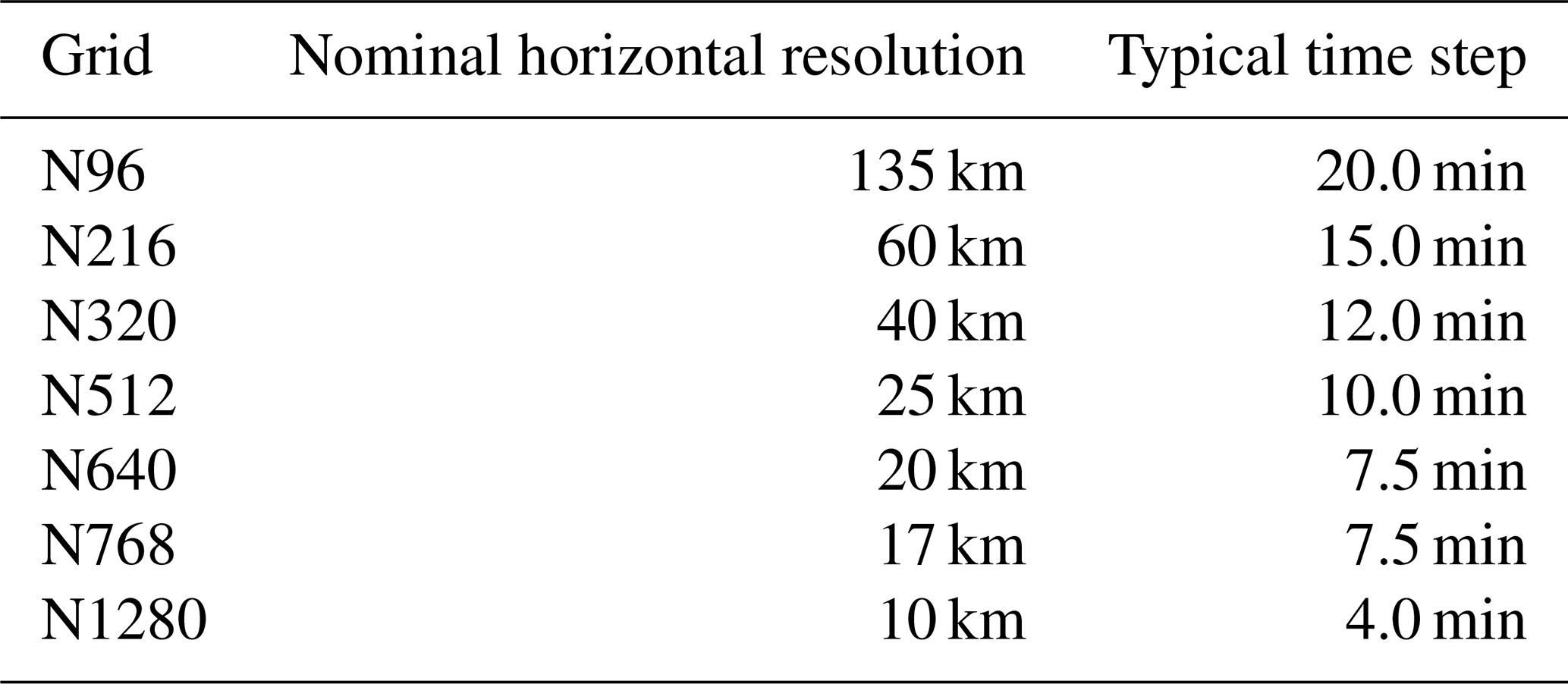
With ENDGame, the UM uses a nested iterative structure for each atmospheric time step within which processes are split into an outer loop and an inner loop. The semi-Lagrangian departure point equations are solved within the outer loop using the latest estimates for the wind variables. Appropriate fields are then interpolated to the updated departure points. Within the inner loop, the Coriolis, orographic and non-linear terms are solved along with a linear Helmholtz problem to obtain the pressure increment. The Helmholtz problem is solved using a multigrid method as described in Sect. 3.7.1. Latest estimates for all variables are then obtained from the pressure increment via a back-substitution process; see Wood et al. (2014) for details. The physical parametrisations are split into slow processes (radiation, large-scale precipitation and gravity wave drag) and fast processes (atmospheric boundary layer turbulence, convection and surface coupling). The slow processes are treated in parallel and are computed once per time step before the outer loop. The source terms from the slow processes are then added on to the appropriate fields before interpolation. The fast processes are treated sequentially and are computed in the outer loop using the latest predicted estimate for the required variables at the next, n+1 time step. A summary of the atmospheric time step is given in Algorithm 1. In practice two iterations are used for each of the outer and inner loops so that the Helmholtz problem is solved four times per time step. The prognostic aerosol scheme is included via a call to the UK Chemistry and Aerosol (UKCA) code after the main atmospheric time step; this call is currently performed once per hour. Finally, Table 1 contains the typical length of time step used for a range of horizontal resolutions.

Algorithm 1 Iterative structure of time step n+1. Here, we use two inner and two outer loops (L=2, M=2).

1:

Given the solution at time step n, let the first estimate for a prognostic variable F at time level n+1 be $F^{n+\mathrm{1}}=F^n$

2:

Compute slow parametrised processes and time level n forcings $R_F^n$

3:

4:

for $m=\mathrm{1},M$ do {departure (outer-loop) iteration}

5:

Solve the trajectory equations to compute the next estimate of the departure points using the time level n and the latest estimate for time level n+1 wind fields

6:

Interpolate $R_F^n$ to departure points

7:

Compute time level n+1 predictors F^*

8:

Compute fast parametrised processes using latest n+1 predictor F^*

9:

Evaluate time level n component of Helmholtz right hand side ℜⁿ

10:

11:

for $l=\mathrm{1},L$ do {non-linear (inner-loop) iteration}

12:

Evaluate non-linear and Coriolis terms $R_F^{*}$

13:

Evaluate time level n+1 component of Helmholtz right hand side ℜ^*

14:

Solve the Helmholtz problem for the pressure increment π^′ and hence obtain the next estimate for ${\mathit{\pi }}^{n+\mathrm{1}}\equiv {\mathit{\pi }}^n+{\mathit{\pi }}^{\prime }$

15:

Obtain the other prognostic variables at time level n+1 via back-substitution

16:

end for

17:

18:

end for

Table 1 Typical time step for a range of horizontal resolutions.

2.3 Solar and terrestrial radiation

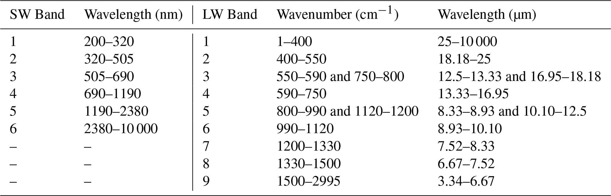
Shortwave (SW) radiation from the Sun is absorbed and reflected in the atmosphere and at the Earth's surface and provides energy to drive the atmospheric circulation. Longwave (LW) radiation is emitted from the planet and interacts with the atmosphere, redistributing heat, before being emitted into space. These processes are parametrised via the radiation scheme, which provides prognostic atmospheric temperature increments, prognostic surface fluxes and additional diagnostic fluxes. The SOCRATES (https://code.metoffice.gov.uk/trac/socrates, last access: 2 February 2026) radiative transfer scheme (Edwards and Slingo, 1996; Manners et al., 2015) is used for GA8. Solar radiation is treated in 6 SW bands and thermal radiation in 9 LW bands, as outlined in Table 2. Gaseous absorption uses the correlated-k method with newly derived coefficients for all gases (except where indicated below) based on the HITRAN 2012 spectroscopic database (Rothman et al., 2013). Scaling of absorption coefficients uses a look-up table of 59 pressures with 5 temperatures per pressure level based around a mid-latitude summer profile. The method of equivalent extinction (Edwards, 1996; Amundsen et al., 2017) is used for minor gases in each band. The water vapour continuum is represented using laboratory results from the CAVIAR project (Continuum Absorption at Visible and Infrared wavelengths and its Atmospheric Relevance) between 1 and 5 µm (Ptashnik et al., 2011, 2012) and version 2.5 of the Mlawer–Tobin_Clough–Kneizys–Davies (MT_CKD-2.5) model (Mlawer et al., 2012) at other wavelengths.

Table 2 Spectral bands for the treatment of incoming solar (SW) radiation (left) and thermal (LW) radiation (right).

Forty-one (41) k terms are used for the major gases in the SW bands. Absorption by water vapour (H₂O), carbon dioxide (CO₂), ozone (O₃), oxygen (O₂), nitrous oxide (N₂O) and methane (CH₄) is included. Ozone cross-sections for the ultra-violet and visible come from Serdyuchenko et al. (2014) and Gorshelev et al. (2014), along with Brion-Daumont-Malicet (Daumont et al., 1992; Malicet et al., 1995) for the far-UV. In the first SW band, a single k-term is calculated for each 20 nm sub-interval from 200 to 320 nm, and in band 2, a single k-term is calculated for each of the sub-intervals 320–400 and 400–505 nm. This allows the incoming solar flux to be supplied on these finer wavelength bands for experiments concerning solar spectral variability. The solar spectrum uses data from NRLSSI (Lean et al., 2005) as recommended by the SPARC/SOLARIS (http://solarisheppa.geomar.de/ccmi, last access: 2 February 2026) group. A mean solar spectrum for the period 2000–2011 is used when a varying spectrum is not invoked.

Eighty-one (81) k terms are used for the major gases in the LW bands. Absorption by H₂O, O₃, CO₂, CH₄, N₂O, CFC-11 (CCl₃F), CFC-12 (CCl₂F₂) and HFC134a (CH₂FCF₃) is included. For climate simulations, the atmospheric concentrations of CFC-12 and HFC134a are adjusted to represent absorption by all the remaining trace halocarbons. The treatment of CO₂ absorption for the peak of the 15 µm band (LW band 4) is as described in Zhong and Haigh (2000). An improved representation of CO₂ absorption in the “window” region (8–13 µm) provides a better forcing response to increases in CO₂ (Pincus et al., 2015). The method of “hybrid” scattering is used in the LW which runs full scattering calculations for 27 of the major gas k-terms (where their nominal optical depth is less than 10 in a mid-latitude summer atmosphere). For the remaining 54 k-terms (optical depth > 10) much cheaper non-scattering calculations are run.

Of the major gases considered, only H₂O is prognostic; O₃ uses a zonally symmetric climatology, whilst other gases are prescribed using either fixed or time-varying mass mixing ratios and assumed to be well mixed.

Absorption and scattering by the following prognostic aerosol species (the representation of which is discussed in Sect. 2.10 below) are included in both the SW and LW using the UKCA-Radaer scheme: sulphate, black carbon, organic carbon and sea salt. The aerosol scattering and absorption coefficients and asymmetry parameters are precomputed for a wide range of plausible Mie parameters and stored in look-up tables for use during run-time when the atmospheric chemical composition, including mean aerosol particle radius and water content are known. As the aerosol species are internally mixed within the modal aerosol scheme (see Table 4 in Walters et al., 2019) the refractive indices of each mode are calculated online as a volume weighted mean of the component species contributing to that mode. The component refractive indices are documented in the Appendix of Bellouin et al. (2013). Nucleation mode particles are neglected as they are not expected to contribute significantly to the atmospheric optical properties. The parametrisation of cloud droplets is described in Edwards and Slingo (1996) using the method of “thick averaging”. Padé fits are used for the variation with effective radius, which is computed from the number of cloud droplets. In configurations using prognostic aerosol, cloud droplet number concentrations are not calculated within the radiation scheme itself but are calculated by the UKCA-Activate scheme (West et al., 2014), which is based on the activation scheme of Abdul-Razzak and Ghan (2000). In NWP configurations, cloud droplet number concentration is not calculated within the radiation scheme but instead is calculated via the method described in Jones et al. (1994); this is done to reduce computational cost. Note that in simulations using climatological rather than prognostic aerosol, the approach described here is not yet available and instead we use CLASSIC (Coupled Large-scale Aerosol Simulator for Studies in Climate, Bellouin et al., 2011) aerosol climatologies and the calculation of optical properties and cloud droplet concentrations described in Sect. 2.3 of Walters et al. (2017). Both prognostic and climatological simulations of mineral dust use the CLASSIC scheme. The parametrisation of ice crystals is described in Baran et al. (2016). Full treatment of scattering is used in both the SW and LW. The sub-grid cloud structure is represented using the Monte Carlo Independent Column Approximation (McICA) (Pincus et al., 2003 with enhancements and implementation described in Hill et al., 2011), with the parametrisation of subgrid-scale water content variability described in Hill et al. (2015).

Full radiation calculations are made every hour using the instantaneous cloud fields and a mean solar zenith angle for the following 1 h period. Corrections are made for the change in solar zenith angle on every model time step as described in Manners et al. (2009). The emissivity and the albedo of the surface are set by the land surface model. The direct SW flux at the surface is corrected for the angle and aspect of the topographic slope as described in Manners et al. (2012).

2.4 Large-scale precipitation

The formation and evolution of precipitation due to grid scale processes is the responsibility of the large-scale precipitation – or microphysics – scheme, whilst small-scale precipitating events are handled by the convection scheme. The microphysics scheme has prognostic input fields of temperature, moisture, cloud and precipitation from the end of the previous time step, which it modifies in turn. The microphysics used is a single moment scheme based on Wilson and Ballard (1999), with extensive modifications. The warm-rain scheme is based on Boutle et al. (2014b), and includes a prognostic rain formulation, which allows three-dimensional advection of the precipitation mass mixing ratio, and an explicit representation of the effect of sub-grid variability on autoconversion and accretion rates (Boutle et al., 2014a). We use the rain-rate dependent particle size distribution of Abel and Boutle (2012) and fall velocities of Abel and Shipway (2007), which combine to allow a better representation of the sedimentation and evaporation of small droplets. We also make use of multiple sub-time steps of the precipitation scheme, with one call to the scheme for every two minutes of model time step. This is required to achieve a realistic treatment of in-column evaporation. With prognostic aerosol, we use the UKCA-Activate aerosol activation scheme (West et al., 2014) to provide the cloud droplet number for autoconversion, where particles from the soluble aerosol modes are activated into cloud droplets. The soluble modes comprise sulphate, sea salt, black carbon and organic carbon but with black carbon remaining hydrophobic within the internally mixed particles. The Aitken insoluble mode comprised of black carbon and organic carbon also participates in activation to form cloud condensation nuclei. When using climatological aerosol, the cloud droplet number is the same as that used in the radiation scheme. Ice cloud parametrisations use the generic size distribution of Field et al. (2007) and mass-diameter relations of Cotton et al. (2013).

2.5 Large-scale cloud

Cloud appears on sub-grid scales well before the humidity averaged over the size of a model grid box reaches saturation. A cloud parametrisation scheme is therefore required to determine the fraction of the grid box which is covered by cloud, and the amount and phase of condensed water contained in this cloud. The formation of cloud will convert water vapour into liquid or ice and release latent heat. The cloud cover and liquid and ice water contents are then used by the radiation scheme to calculate the radiative impact of the cloud and by the large-scale precipitation scheme to calculate whether any precipitation has formed.

The parametrisation used is the prognostic cloud fraction and prognostic condensate (PC2) scheme (Wilson et al., 2008a, b) along with the cloud erosion parametrisation described by Morcrette (2012) and critical relative humidity parametrisation described in Van Weverberg et al. (2016). PC2 uses three prognostic variables for water mixing ratio – vapour, liquid and ice – and a further three prognostic variables for cloud fraction: liquid, ice and mixed-phase. The following atmospheric processes can modify the cloud fields: SW radiation, LW radiation, boundary layer processes, convection, precipitation, small-scale mixing (cloud erosion), advection and changes in atmospheric pressure. The convection scheme calculates increments to the prognostic liquid and ice water contents by detraining condensate from the convective plume, whilst the cloud fractions are updated using the non-uniform forcing method of Bushell et al. (2003). One advantage of the prognostic approach is that cloud can be transported away from where it was created. For example, anvils detrained from convection can persist and be advected downstream long after the convection itself has ceased. The radiative impact of convective cores, which hold condensate not detrained into the environment, is represented by diagnosing a convective cloud amount (CCA) and convective cloud water (CCW) where the convection is active on a particular time-step. The CCA and CCW then get combined with the PC2 cloud fraction and condensate variables before these get passed to McICA to calculate the radiative impact of the combined cloud fields. Finally, the production of supercooled liquid water in a turbulent environment is parametrised following Furtado et al. (2016).

2.6 Sub-grid orographic drag

The effect of local and mesoscale orographic features not resolved by the mean orography, from individual hills through to small mountain ranges, must be parametrised. The smallest scales, where buoyancy effects are assumed to be unimportant, are represented by the explicit orographic stress parametrisation of Wood et al. (2001). The effects of the remainder of the sub-grid orography (on scales where buoyancy effects are important) are parametrised by a drag scheme which represents the effects of low-level flow blocking and the drag associated with stationary gravity waves (mountain waves). This is based on the scheme described by Lott and Miller (1997), but with some important differences, described in more detail in Vosper (2015).

The sub-grid orography is assumed to consist of uniformly distributed elliptical mountains within the grid box, described in terms of a height amplitude, which is proportional to the grid box standard deviation of the source orography data, anisotropy (the extent to which the sub-grid orography is ridge-like, as opposed to circular), the alignment of the major axis and the mean slope along the major axis. The scheme is based on two different frameworks for the drag mechanisms: bluff body dynamics for the flow-blocking and linear gravity waves for the mountain wave drag component.

The degree to which the flow is blocked and so passes around, rather than over the mountains is determined by the Froude number, $F=U/\left(NH\right)$ where H is the assumed sub-grid mountain height (proportional to the sub-grid standard deviation of the source orography data) and N and U are respectively measures of the buoyancy frequency and wind speed of the low-level flow. When F is less than the critical value, F_c, a fraction of the flow is assumed to pass around the sides of the orography, and a drag is applied to the flow within this blocked layer. Mountain waves are generated by the remaining proportion of the layer, which the orography pierces through. The acceleration of the flow due to wave stress divergence is exerted at levels where wave breaking is diagnosed. The kinetic energy dissipated through the flow-blocking drag, the mountain-wave drag and the non-orographic gravity wave drag (see Sect. 2.7 below) is returned to the atmosphere as a local heating term.

2.7 Non-orographic gravity wave drag

Non-orographic sources – such as convection, fronts and jets – can force gravity waves with non-zero phase speed. These waves break in the upper stratosphere and mesosphere, depositing momentum, which contributes to driving the zonal mean wind and temperature structures away from radiative equilibrium. Waves on scales too small for the model to sustain explicitly are represented by a spectral sub-grid parametrisation scheme (Scaife et al., 2002), which by contributing to the deposited momentum leads to a more realistic tropical quasi-biennial oscillation (QBO). The scheme, described in more detail in Walters et al. (2011), represents processes of wave generation, conservative propagation and dissipation by critical-level filtering and wave saturation acting on a vertical wavenumber spectrum of gravity wave fluxes following Warner and McIntyre (2001). Momentum conservation is enforced at launch in the lower troposphere, where isotropic fluxes guarantee zero net momentum, and by imposing a condition of zero vertical wave flux at the model's upper boundary. In between, momentum deposition occurs in each layer where reduced integrated flux results from erosion of the launch spectrum, after transformation by conservative propagation, to match the locally evaluated saturation spectrum.

2.8 Atmospheric boundary layer

Turbulent motions in the atmosphere are not resolved by global atmospheric models, but are important to parametrise in order to give realistic vertical structure in the thermodynamic and wind profiles. Although referred to as the “boundary layer” (BL) scheme, this parametrisation represents mixing over the full depth of the troposphere. The scheme is that of Lock et al. (2000) with the modifications described in Lock (2001) and Brown et al. (2008). It is a first-order turbulence closure mixing adiabatically conserved heat and moisture variables, momentum and tracers. For unstable BLs, diffusion coefficients (K profiles) are specified functions of height within the BL, related to the strength of the turbulence forcing. Two separate K profiles are used, one for surface sources of turbulence (surface heating and wind shear) and one for cloud top sources (radiative and evaporative cooling). The existence and depth of unstable layers is diagnosed initially by two moist adiabatic parcels, one released from the surface, the other from cloud-top. The top of the K profile for surface sources and the base of that for cloud-top sources are then adjusted to ensure that, from the resultant buoyancy flux, the magnitude of the buoyancy consumption of turbulence kinetic energy is limited to a specified fraction of buoyancy production, integrated across the BL. This can permit the cloud layer to decouple from the surface (Nicholls, 1984). This same energetic diagnosis is used to limit the vertical extent of the surface-driven K profile when cumulus convection is diagnosed (through comparison of cloud and sub-cloud layer moisture gradients), except that in this case no condensation is included in the diagnosed buoyancy flux because that part of the distribution is handled by the convection scheme (which is triggered at cloud base). Mixing across the top of the BL is through an explicit entrainment parametrisation that can either be resolved across a diagnosed inversion thickness or, if too thin, is coupled to the radiative fluxes and the dynamics through a sub-grid inversion diagnosis. If the thermodynamic conditions are right, cumulus penetration into a stratocumulus layer can generate additional turbulence and cloud-top entrainment in the stratocumulus by enhancing evaporative cooling at cloud top. In convective BLs, the scheme includes additional non-local fluxes of heat and momentum that represent the efficient mixing by convective thermals. These generate the vertically uniform potential temperature and wind profiles seen in observations. Primarily for stable BLs and in the free troposphere, diffusion coefficients are also calculated using a local Richardson number scheme based on Smith (1990), with the final coefficients being the maximum of this and the non-local ones described above. The stability dependence in unstable BLs uses the “conventional function” of Brown (1999) that gives only weak enhancement over neutral mixing, as we expect the non-local scheme to be most appropriate in this regime. The stability dependence in stable BLs is given by the “sharp” function over sea and by the “MES-tail” function over land (which matches linearly between an enhanced mixing function at the surface and “sharp” at 200 m and above), as defined in Brown et al. (2008). This additional near-surface mixing is motivated by the effects of surface heterogeneity, such as those described in McCabe and Brown (2007). The resulting diffusion equation is solved implicitly using the monotonically damping, second-order-accurate, unconditionally stable numerical scheme of Wood et al. (2007). The kinetic energy dissipated through the turbulent shear stresses is returned to the atmosphere as a local heating term.

2.9 Convection

The convection scheme represents the sub-grid scale transport of heat, moisture and momentum associated with cumulus cloud within a grid box. The UM uses a mass flux convection scheme based on Gregory and Rowntree (1990) with various extensions to include down-draughts (Gregory and Allen, 1991) and convective momentum transport (CMT). The current scheme consists of three stages: (i) convective diagnosis to determine whether convection is possible from the BL; (ii) a call to the shallow or deep convection scheme for all points diagnosed deep or shallow by the first step; and (iii) a call to the mid-level convection scheme for all grid points.

The diagnosis of shallow and deep convection is based on an undilute parcel ascent from the near surface for grid boxes where the surface buoyancy flux is positive and forms part of the BL diagnosis (Lock et al., 2000). Shallow convection is then diagnosed if the following conditions are met: (i) the parcel attains neutral buoyancy below 2.5 km or below the freezing level, whichever is higher, and (ii) the air in model levels forming a layer of order 1500 m above this has a mean upward vertical velocity less than 0.02 m s⁻¹. Otherwise, convection diagnosed from the BL is defined as deep.

The deep convection scheme differs from the original Gregory and Rowntree (1990) scheme in using a convective available potential energy (CAPE) closure based on Fritsch and Chappell (1980). Mixing detrainment rates now depend on relative humidity and forced detrainment rates adapt to the buoyancy of the convective plume (Derbyshire et al., 2011). The entrainment is dependent on the level of recent convective activity as described in Willett and Whitall (2017) and summarised in Sect. 3.5.3. A numerically a more stable version of the Gregory et al. (1997) CMT scheme is used which is described in Sect. 3.5.2.

The shallow convection scheme uses a closure based on Grant (2001) and has relatively large entrainment rates consistent with cloud-resolving model (CRM) simulations of shallow convection. The shallow CMT uses flux–gradient relationships derived from CRM simulations of shallow convection (Grant and Brown, 1999).

The mid-level scheme operates on any instabilities found in a column above the top of deep or shallow convection or above the lifting condensation level. The scheme is largely unchanged from Gregory and Rowntree (1990) but uses the numerically more stable version of the Gregory et al. (1997) CMT scheme and a CAPE closure. The mid-level scheme typically operates overnight over land when convection from the stable BL is no longer possible or in the region of strong dynamical forcing such as tropical cylcones or mid-latitude storms. Other cases of mid-level convection tend to remove instabilities over a few levels and do not produce much precipitation.

Condensed water in the updraught parcel is converted to precipitation when it exceeds a critical value. This critical value is simply parametrised as a fixed fraction of the local environmental saturated specific humidity ($\mathrm{0.35}{q}_{\mathrm{sat}}^{\mathrm{Env}}$) bounded by fixed upper (1 g kg⁻¹) and lower limits (0.4 g kg⁻¹) (see Walters et al., 2014, Eq. 7). The convective precipitation may either evaporate within the downdraught, evaporate in the environment below cloud base, or reach the surface. Detrained convective condensate is converted directly to large-scale cloud condensate and the large-scale cloud fraction is updated using the “injection forcing” method described in Wilson et al. (2008a).

The timescale for the CAPE closure, which is used for deep and mid-level convection schemes, varies according to the large-scale vertical velocity. The values used vary from a minimum value of 30 min when the ascent is relatively strong, to a maximum of either 4 h for mid-level convection, or the minimum of either 4 h or a time scale from a surface flux closure for deep convection.

The convection scheme is sub-stepped with two sequential calls to the shallow, mid-level and deep convection schemes per model timestep, with each call using half the full model timestep. This was originally introduced to improve the numerical stability of the model.

To mitigate against the detrimental dynamical effects of intermittency within the convection scheme, the potential temperature and humidity increments from the convection scheme as seen by the rest of the model are damped in time with a damping timescale of 45 min.

2.10 Atmospheric aerosols

As discussed in Walters et al. (2011), the precise details of the modelling of atmospheric aerosols and chemistry is considered as a separate component of the full Earth system and remains outside the scope of this document. The aerosol species represented and their interaction with the atmospheric parametrisations is, however, part of the Global Atmosphere component and is therefore included. GA8 provides the option to use either prognostic aerosols or climatological aerosols with the choice being dependent on the needs of the application.

If prognostic aerosols are used this is done using the GLOMAP-mode (Global Model of Aerosol Processes) aerosol scheme described in Mann et al. (2010) with updates described in Mulcahy et al. (2018). The scheme simulates speciated aerosol mass and number in 4 soluble modes covering the sub-micron to super-micron aerosol size ranges (nucleation, Aitken, accumulation and coarse modes) as well as an insoluble Aitken mode. The prognostic aerosol species represented are sulphate, black carbon, organic carbon and sea salt. For more details see Walters et al. (2019) and Mulcahy et al. (2020).

If climatological aerosols are used this is done so using three-dimensional monthly climatologies for each aerosol species to model both the direct and indirect aerosol effects. In GA8, we continue to use the use climatologies based on the CLASSIC aerosol scheme (Bellouin et al., 2011) as described in Walters et al. (2017), which has a different representation of aerosol species and their direct and indirect aerosol effects compared to GLOMAP-mode. Future GA releases aim to use aerosol climatologies based on GLOMAP and will provide greater consistency between prognostic and climatological representations of the aerosol.

In addition to the treatment of these tropospheric aerosols, we include simple representations of the radiative impact of stratospheric aerosols, such as those related to injections of SO2 from explosive volcanic eruptions, because the GLOMAP-mode and CLASSIC climatologies do not sufficiently capture sources of stratospheric aerosols. In NWP simulations this is prescribed using a coarse-grain stratospheric aerosol climatology based on Cusack et al. (1998), while in climate simulations we apply the CMIP6 forcing of Thomason et al. (2018) as described in Sect. 3.2.1 of Sellar et al. (2020). Mineral dust is simulated using the CLASSIC dust scheme described in Woodward (2011). We also include the production of stratospheric water vapour via a simple methane oxidation parametrisation (Untch and Simmons, 1999).

2.11 Surface flux exchange, land surface and hydrology: Global Land 9.0

The exchange of fluxes between the surface (land, sea and sea-ice) and the atmosphere is an important mechanism for heating and moistening the atmospheric BL. In addition, the exchange of CO₂ and other greenhouse gases plays a significant role in the climate system. The hydrological state of the land surface contributes to impacts such as flooding and drought as well as providing freshwater fluxes to the ocean, which influences ocean circulation. The Global Land configuration uses a community land surface model, JULES (Best et al., 2011; Clark et al., 2011), to model all of these processes in atmosphere/land only and in coupled applications.

In atmosphere/land only applications, the sea surface temperature (SST) is prescribed via an ancillary file. The sea-ice is simply modelled within JULES as a single layer of ice with fixed thickness and areal heat capacity, with the top boundary condition given by the heat flux into the sea-ice and a bottom boundary set to the freezing temperature of sea water. The surface temperature is determined from the surface energy balance using the gradient between the surface and ice temperatures, with a fixed thermal conductivity. Although the details of coupling between the atmosphere, ocean and sea-ice models when running in coupled simulations lie outside the scope of this paper, it is useful to note, however, where the boundaries lie between JULES, and the ocean and sea-ice components when GA8GL9 is run in coupled mode as part of GC4. In GC4, the SST is set to be equal to the temperature of the 1 m-thick, top ocean layer, which is calculated within the ocean model, with JULES being used to calculate the surface fluxes that are subsequently passed back to the ocean. Over the sea-ice, JULES is used to calculate both the skin temperature of the top sea-ice layer and the surface fluxes, because this has been shown to be both more accurate and more numerically stable than calculating them within the sea-ice model (West et al., 2016).

A tile approach is used to represent sub-grid scale heterogeneity of the land-surface (Essery et al., 2003b), with the surface of each land grid box subdivided into five types of vegetation (broadleaf trees, needle-leaved trees, temperate C₃ grass, tropical C₄ grass and shrubs) and four non-vegetated surface types (urban areas, inland water, bare soil and land ice). The ground beneath vegetation is coupled to the vegetation canopy by LW radiation and turbulent sensible heat exchanges. JULES also uses a canopy radiation scheme to represent the penetration of light within the vegetation canopy and its subsequent impact on photosynthesis (Mercado et al., 2007). The canopy also interacts with falling snow. Snow buries the canopy for most vegetation types, but the interception of snow by both needle-leaved and broad-leaved trees is represented with separate snow stores on the canopy and on the ground. This impacts the surface albedo, the snow sublimation and the snow melt (Essery et al., 2003a). The vegetation canopy code has been adapted for use with the urban surface type by defining an “urban canopy” with the thermal properties of concrete (Best, 2005), and evaluates well for the surface heat and moisture fluxes (Grimmond et al., 2011; Lipson et al., 2023).

Following Best et al. (2011), this canopy approach has also been adopted for the representation of inland water³. By defining an “inland water canopy” and setting the thermal characteristics to those of a suitable mixed layer depth of water (≈5 m), a better diurnal and seasonal cycle for the surface temperature is achieved than for the original “permanently saturated soil” approach (Rooney and Jones, 2010). The depth of the water in the canopy is held fixed, but global water conservation is pragmatically ensured by a small global adjustment to the water content of the deepest soil level (with appropriate checks to avoid negative values or supersaturation) in response to water fluxes into and out of the inland water canopies. The surface below the inland water canopy is essentially decoupled from the canopy, and hence it plays no role in the model's evolution.

Following Best et al. (2011) and as described in more detail in Wiltshire et al. (2020), land ice is represented by using the soil scheme with the soil parameters set to appropriate values for ice, i.e., the thermal characteristics are set to those of ice, whilst the other soil parameters are set to zero. This means that it is not possible to have both land ice and other surface types in the same grid box, as they share the same soil profile; hence, if land ice is present in the model, then it must cover 100 % of the grid box. Furthermore, to reduce the likelihood of small scale sharp horizontal gradients which could lead to numerical problems, only large areas of land ice are permitted in the model, e.g. in most climate simulations, only Antarctica and Greenland are included. Land ice is typically initiated at the start of integrations with a large amount of overlying snow to ensure that not all of the snow can be removed through sublimation or melt during the simulation. In addition, as the lateral transfer of snow by glacial movement is not represented in the model, it is possible to accumulate very large amounts of snow. However, this does not adversely impact on the surface energy balance. The surface temperature is not allowed to go above the melting temperature, but instead the associated energy is used to melt the snow. Infiltration of this snow melt, along with any liquid precipitation, is not permitted into the land ice, but is directed to surface runoff.

Surface fluxes are calculated separately on each tile using surface similarity theory. In stable conditions we use the stability functions of Beljaars and Holtslag (1991), whilst in unstable conditions we take the functions from Dyer and Hicks (1970). The effects on surface exchange of both BL gustiness (Godfrey and Beljaars, 1991) and deep convective gustiness (Redelsperger et al., 2000) are included. Temperatures at 1.5 m and winds at 10 m are interpolated between the model's grid levels using the same similarity functions, but a parametrisation of transitional decoupling in very light winds is included in the calculation of the 1.5 m temperature.

The roughness length for the bare soil is specified via an ancillary file that is based on Prigent et al. (2012) and the roughness lengths for all other land type are explicitly specified. Over the sea surface the COARE (Coupled Ocean–Atmosphere Response Experiment) 4.0 (Edson, 2009) momentum roughness length parametrisation is used. The drag coefficient over the sea at very high wind speeds (greater than 33 m s⁻¹) is reduced as described in Sect. 3.1.3. The form drag for marginal ice uses the explicit representation from Lupkes et al. (2012) as described in Sect. 3.1.1.

SW radiation fluxes use a “first guess” snow-free albedo for each land surface type, which can then be nudged towards an imposed grid box mean value taken from a climatology. This nudging is not performed in either climate change simulations or any other simulations with dynamic vegetation. The grid-box mean albedo of the land surface is further modified in the presence of snow. The albedo of the ocean surface is a function of the wavelength, the solar zenith angle, the 10 m wind speed and the chlorophyll content according to the Jin et al. (2011) parametrisation. The emitted LW radiation is calculated using a prescribed emissivity for each surface type.

Soil processes are represented using a 4-layer scheme for the heat and water fluxes with hydraulic relationships taken from van Genuchten (1980). These four soil layers have thicknesses from the top down of 0.1, 0.25, 0.65 and 2.0 m. The impact of moisture on the thermal characteristics of the soil is represented using a simplification of Johansen (1975), as described in Dharssi et al. (2009). The energetics of water movement within the soil is accounted for, as is the latent heat exchange resulting from the phase change of soil water from liquid to solid states. Sub-grid scale heterogeneity of soil moisture is represented using the Large-Scale Hydrology approach (Gedney and Cox, 2003), which is based on the topography-based rainfall-runoff model TOPMODEL (Beven and Kirkby, 1979). This enables the representation of an interactive water table within the soil that can be used to represent wetland areas, as well as increasing surface runoff through heterogeneity in soil moisture driven by topography.

A river routing scheme is used to route the total runoff (from all land surface types including land ice) from inland grid points both out to the sea and to inland basins (where it can flow back into the soil moisture). If the soil at inland basin points becomes saturated and hence unable to hold more water, the resultant runoff is pragmatically redirected evenly across all sea outflow points. The resulting increase in the river outflow is always very small and does not affect the ocean salinity structure in any significant way, but importantly this process ensures global water conservation which is an important criterion for global climate models. In coupled model simulations the resulting freshwater outflow is passed to the ocean, where it is an important component of the thermohaline circulation, whilst in atmosphere/land-only simulations this ocean outflow is purely diagnostic. River routing calculations are performed using the TRIP (Total Runoff Integrating Pathways) model (Oki and Sud, 1998), which uses a simple advection method (Oki, 1997) to route total runoff along prescribed river channels on a 1° × 1° grid using a 3 h time step. Land surface runoff accumulated over this time step is mapped onto the river routing grid prior to the TRIP calculations, after which soil moisture increments and total outflow at river mouths are mapped back to the atmospheric grid (Falloon and Betts, 2006). This river routing model is not currently being used in NWP implementations of the Global Atmosphere/Land and hence any runoff is purely diagnostic and “lost” from the model's water budget.

2.12 Stochastic physics

A key component of many Ensemble Prediction Systems (EPSs) is the use of stochastic physics schemes to represent model error emerging from unrepresented or coarsely resolved processes such as numerical diffusion or fluctuations in the impact of physical parametrisations on the large-scale fields. The addition of unresolved variability around the deterministic solution adds spread between ensemble members and has been shown to improve ensemble predictions in the medium range (Palmer et al., 2009; Tennant et al., 2011) as well as on seasonal (Weisheimer et al., 2011) and decadal time scales (Doblas-Reyes et al., 2009). The increase in the model's internal variability also helps to improve the model's climatology, through a noise-drift induced process. In particular, there is strong evidence of the positive impact of stochastic physics schemes on specific processes such as mid-latitude blocking (Berner et al., 2012), the Madden–Julian Oscillation (MJO, Madden and Julian, 1971; Weisheimer et al., 2014) and North Atlantic weather regimes (Dawson and Palmer, 2015).

In GA8, we use a standardised package of stochastic physics schemes (Sanchez et al., 2016) based on an improved version of the Stochastic Kinetic Energy Backscatter scheme version 2 (SKEB2, Tennant et al., 2011) and the Stochastic Perturbation of Tendencies scheme (SPT) with additional constraints designed to conserve energy and water. SKEB2 adds forcing to the large-scale flow to represent the backscatter of small-scale kinetic energy lost via numerical diffusion, whilst SPT stochastically scales the output of physical parametrisations to represent variability about their mean predictions. Despite the positive impact of model error stochastic physics schemes on EPS and climate model performance by making probability forecasts more statistically reliable and reducing the error of the ensemble mean, their formulations fundamentally add noise which degrades forecast skill when run in deterministic mode (Sanchez et al., 2016). For these reasons, these schemes are not used in deterministic forecast systems, which are designed to forecast the best possible single prediction of the atmosphere’s future state.

2.13 Global atmospheric energy correction

Long climate simulations of the Unified Model include an energy correction scheme, designed to ensure that numerical errors, inconsistent geometric assumptions and missing processes do not lead to any spurious drift in the atmosphere's total energy. The scheme accumulates the net flux of energy through the upper and lower boundaries of the atmosphere over a period of 1 d and calculates the difference between this and the change in the atmosphere's internal energy. Any drift is compensated by the addition of a globally uniform temperature increment, which is applied every time step for the following day. In GA8GL9, the magnitude of these corrections is typically $\lesssim +\mathrm{0.7}$ W m⁻².

2.14 Ancillary files and forcing data

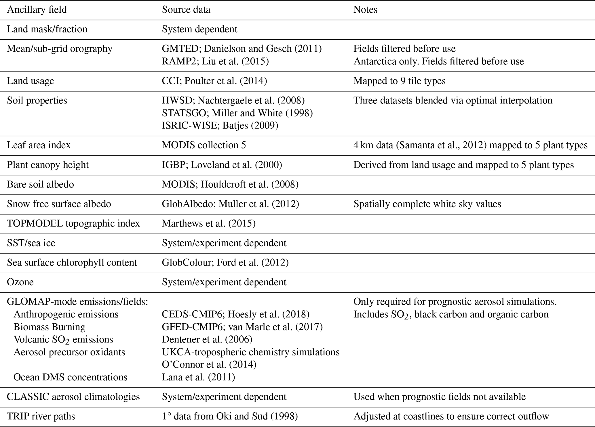
In the UM, the characteristics of the lower boundary, the values of climatological fields and the distribution of natural and anthropogenic emissions are specified using ancillary files. Use of correct ancillary file inputs can play as important a role in the performance of a system as the correct choice of many options in the parametrisations described above. For this reason, we consider the source data and processing required to create ancillaries as part of the definition of the Global Atmosphere/Land configurations. Table 3 contains the main ancillaries used as well as references to the source data from which they are created.

Danielson and Gesch (2011)Liu et al. (2015)Poulter et al. (2014)Nachtergaele et al. (2008)Miller and White (1998)Batjes (2009)(Samanta et al., 2012)Loveland et al. (2000)Houldcroft et al. (2008)Muller et al. (2012)Marthews et al. (2015)Ford et al. (2012)Hoesly et al. (2018)van Marle et al. (2017)Dentener et al. (2006)O'Connor et al. (2014)Lana et al. (2011)Oki and Sud (1998)

Table 3 Source datasets used to create standard ancillary files used in GA8GL9.

3 Developments since GA7GL7

The subject of this paper, GA8GL9, builds upon GA7GL7 (Walters et al., 2019) which was released in January 2016. GA8GL9 consolidates the changes made for the climate specific branch configuration GA7.1GL7.1 (Walters et al., 2019) and NWP specific GA7.2GL8.1 (Willett et al., 2023) apart from system specific tunings or where a newer science option has made change in previous branch configurations redundant. In particular the changes documented in this section with GMED tickets #192, #197, #257, #272 were originally included in GA7.1GL7.1 and those with GMED tickets #194, #207, #251, #290, #301, #324, #434, #474, #476 and #531 were originally included in GA7.2GL8.1. In addition to the consolidation of changes from the branch configuration, GA8GL9 also includes changes to most areas of the science. This section gives a description of all the changes added between GA7GL7 and GA8GL9 including those that were previously included in branch configurations.

3.1 Surface flux exchange, land surface and hydrology

3.1.1 Revised roughness parametrisation for marginal ice (GMED ticket #194)

The parametrisation of the roughness of marginal ice (i.e. the transition zone between pack ice and open sea) has been updated with the following changes being made:

• In GL7 the exchange and drag coefficients over sea-ice were interpolated between values representative of pack ice, the marginal ice and open sea. In GL9 this is replaced by explicit representation of form drag for marginal ice from Lupkes et al. (2012), which was validated by Elvidge et al. (2016), and using the extension from Lupkes and Gryanik (2015) to account for stability.

• The conductivity of snow on sea-ice is reduced from 0.50 to 0.256 W m⁻¹ K⁻¹ to be consistent with the relationship between snow conductivity and density used in the multilayer snow scheme taken from Calonne et al. (2011) and the assumed density for snow on sea ice (330 kg m⁻³).

• The conductivity of sea ice is reduced to from 2.63 to 2.09 W m⁻¹ K⁻¹

Renfrew et al. (2019) evaluated the changes to the marginal ice drag. They demonstrated that biases and root mean square errors (RMSEs) in temperature and winds were reduced with respect to aircraft observations both over and downstream of the marginal ice zone.

3.1.2 Modifications to the rate of growth of snow grains (GMED ticket #251)

The size of snow grains affects the albedo of the snow with larger grains being darker. Earlier configurations used the parametrisation of snow grains from Marshall (1989) which was developed using continental data and did not represent the very low temperatures of Antarctica. In GL9, this is replaced by the equitemperature part of the scheme described by Taillandier et al. (2007) which predicts a slower rate of growth at colder temperatures, so increasing the albedo under typical Antarctic conditions. In addition, the calculation of the grain size during relayering of the snowpack has been modified to make it more consistent with conservation of specific surface area. Increasing the albedo over Antarctica reduces the near surface temperatures; this ultimately results in reduced circulation errors and substantially improved forecast performance in the southern hemisphere in austral summer. Increasing the albedo over Antarctica increases the error slightly relative to CERES-EBAF, but it is believed that CERES-EBAF is too dark in this region (John M. Edwards, personal communication, August 2023).

3.1.3 Improved drag at high wind speeds (GMED ticket #324)

Although the precise behaviour of the drag at high wind speeds is not fully understood, it is clear that extrapolating standard parametrisations from lower wind speeds gives excessive drag. Indeed, experimental evidence shows that the drag not only saturates at higher wind speeds but actually decreases as the wind speed increases (Donelan et al., 2004; Donelan, 2018; Curcic and Haus, 2020). This change limits the drag coefficient to $\mathrm{3}\times {\mathrm{10}}^{-\mathrm{3}}$ when the neutral wind speed is below 33 m s⁻¹, and gradually reduces it between wind speeds of 33 and 55 m s⁻¹ where it reaches a limiting value of $\mathrm{2}\times {\mathrm{10}}^{-\mathrm{3}}$. This provides good consistency with the experimental estimates. The primary benefit of this development is seen in simulations of tropical cyclones at high resolutions where the drag is reduced and predicted wind speeds are beneficially increased.

3.1.4 GL9 drag package (GMED ticket #435)

A package of land surface changes was developed with the aim of removing the need to use an aggregate surface tile in NWP, improving the large-scale circulation and reducing the differences between the representation of the land-surface in the global and regional configurations. It is described in detail in Williams et al. (2020), but a brief summary of the changes is as follows:

• A combination of GMTED (Danielson and Gesch, 2011) and RAMP2 (Liu et al., 2015) datasets replace GLOBE30 (Hastings et al., 1999) in the generation of the orography ancillaries. A 6th order low-pass filter as described in Raymond and Garder (1988) is used to smooth the source dataset, and derive the mean and subgrid orography fields. In GL9 the filter parameters are modified so that the cut off frequency is increased and hence substantially more detail is retained in the mean orography at smaller scales (e.g. Fig. 1). The consistency between mean and subgrid orography is also improved.

• Prior to GL9, soil roughness was set to a global constant value, i.e. z0=1 mm, but observations shows that it actually varies by orders of magnitude globally. In GL9 the single constant value is replaced by an ancillary field that is based on Prigent et al. (2012).

• The roughness lengths for momentum for each vegetation type are now explicitly specified rather than determined by the vegetation canopy height. These specified roughness lengths were determined by rearranging the model equations to provide a relationship that depends upon the surface momentum flux and wind speed, and then optimising values for different vegetation types using observational data from FLUXNET sites (Pastorello et al., 2020).

• The land use dataset used to generate the surface tile fractions is updated from IGBP to the newer European Space Agency's Land Cover Climate Change Initiative (ESA CCI) land-cover dataset (Poulter et al., 2014). At the same time an appropriate crosswalk table was developed to map the CCI vegetation fractions to the correct JULES vegetation tile based on Table 2 from Poulter et al. (2014). Additional changes were made so that closed trees and grasslands mapped to 100 % of the appropriate JULES tiles. Open canopies and shrubs tile fraction remained the same as the original table. Grasslands were split appropriately between C3 and C4 using data on C4 fractions from Still et al. (2003). The C4 fraction was used to identify the dominant type of grass, and then the CCI fraction was assigned to either C3 or C4 grass tiles.

• The vegetation canopy radiation model option has been updated which provides a more realistic distribution of diffuse radiation through the vegetation canopy. The ratios of the roughness length for heat to roughness length for momentum have been updated for all vegetation types and non-vegetated surface types.

• The orographic roughness scheme of Wood and Mason (1993) is replaced by the distributed form drag scheme of Wood et al. (2001). Both schemes are designed to represent the turbulent form drag due to small-scale sub-grid hills, but the orographic roughness approach is known to result in unrealistic low values for near-surface wind speeds over orography (Rooney and Bornemann, 2013). The distributed form drag approach reduces this detrimental impact on the near surface winds.

• Prior to GL9, canopy snow was only applied to needle-leaved trees. In GL9 it is also applied to broad-leaved trees. As well as being more realistic, this removes an instability mechanism that was previously occasionally seen in snowy conditions when both tree types are present in the same gridbox.

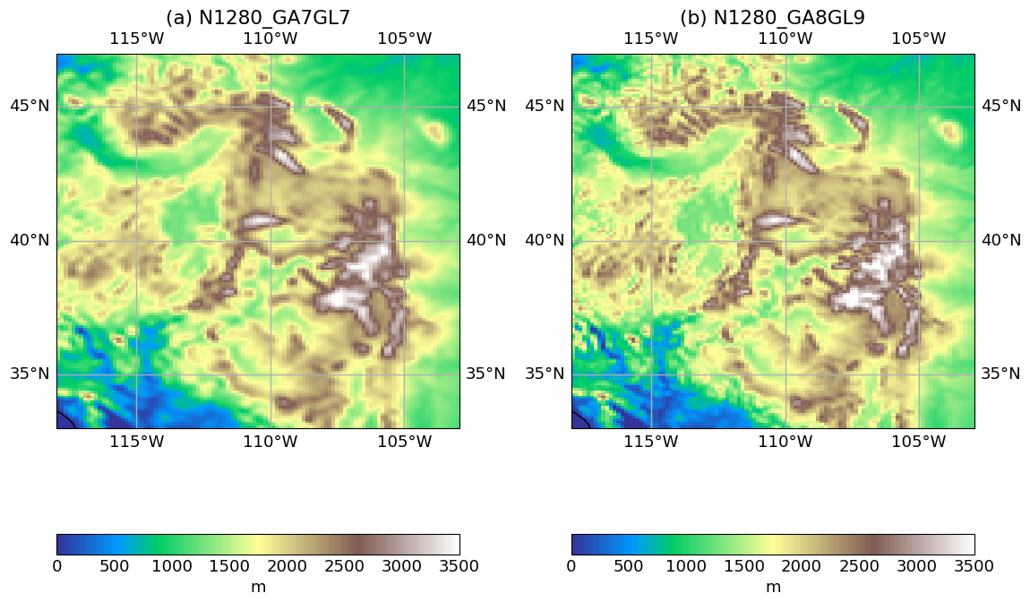
Figure 1 Example N1280 orography from (a) GA7GL7 and (b) GA8GL9 for a region of the eastern USA covering part of the Rocky Mountains.

The package of land surface changes reduces the errors in near-surface winds and temperatures, and hence removes the need to use an aggregate surface tile in NWP applications (Walters et al., 2017, Sect. 4.2.1), which has been a long standing difference between NWP and other applications.

3.2 Solar and terrestrial radiation

3.2.1 Liu cloud droplet spectral dispersion (GMED ticket #192)

In the model the cloud droplet effective radius is calculated as:

$$\begin{array}{}\text{(1)}& {\displaystyle }{r}_{\mathrm{e}}=\mathit{\beta }{\left({\displaystyle \frac{\mathrm{3}L}{\mathrm{4}\mathit{\pi }\mathit{\rho }{N}_{\mathrm{d}}}}\right)}^{\frac{\mathrm{1}}{\mathrm{3}}}\end{array}$$

Where L is the cloud liquid water content, ρ is the density of liquid water, N_d is the cloud droplet number concentration and β is the spectral shape parameter, representing the degree of cloud droplet spectral dispersion. In GA7.0, β is represented by two constants depending on the cloud was over was a land (β=1.14) or ocean (β=1.08) grid-box (Martin et al., 1994), crudely representing “polluted” continental and “pristine” ocean air masses. Following detailed investigations into the aerosol effective radiation forcing (ERF) in GA7.0 (Mulcahy et al., 2018), the spectral dispersion is now calculated following the parametrisation of Liu et al. (2008), i.e.:

$$\begin{array}{}\text{(2)}& {\displaystyle }\mathit{\beta }=a_{\mathit{\beta }}{\left({\displaystyle \frac{L}{N}}\right)}^{-b_{\mathit{\beta }}}\end{array}$$

where a_β=0.07 and b_β=0.14. The impact of this change is to reduce the response of r_e to an increase in aerosol concentration and thereby reduce the magnitude of the aerosol-cloud albedo effect in the model, leading to a weaker (less negative) aerosol ERF in GA7 of approximately 23 % (Mulcahy et al., 2018). The effect of the Liu spectral dispersion on the cloud droplet radius and the bias relative to Clouds and Earth's Radiant Energy System (CERES) Moderate Resolution Imaging Spectrometer (MODIS) is shown in Fig. 2b and d. Overall, the cloud droplet effective radius is generally increased over the northern hemisphere, where GA7 often has the most negative bias, whilst reducing over the southern hemisphere, where GA7 typically has lower negative bias. Overall, this results in the difference from the observation-based estimates becoming more spatially homogeneous.

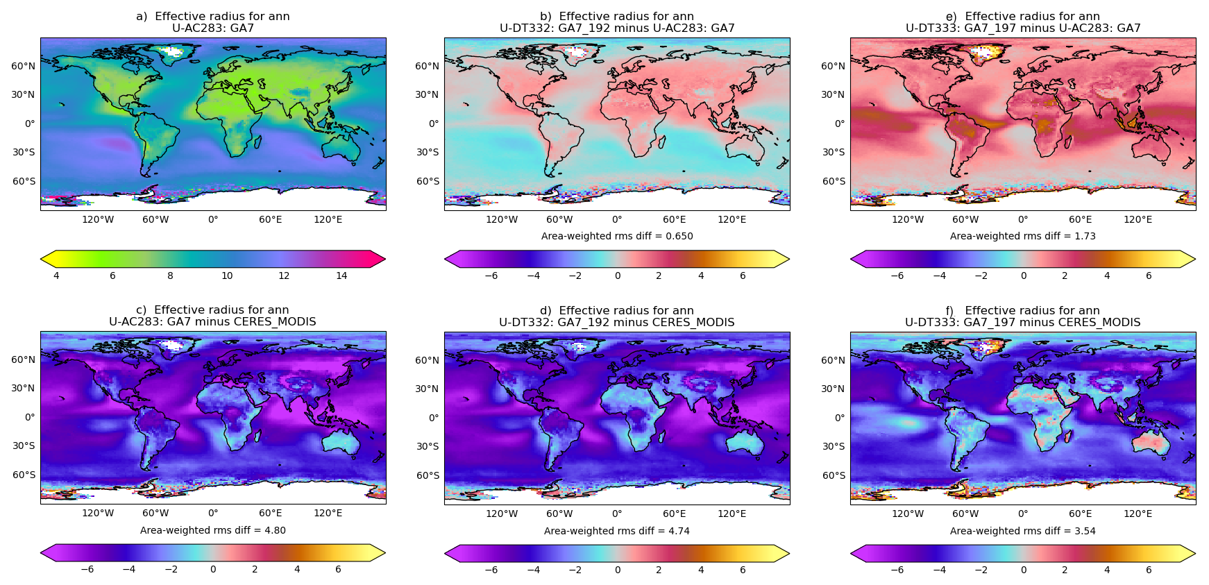
Figure 2 Annual mean cloud droplet effective radius (µm) in the 20 year N96 atmosphere/land only climate simulations compared to Clouds and Earth's Radiant Energy System (CERES) Moderate Resolution Imaging Spectrometer (MODIS) showing (a) GA7GL7, (b) the effect of the Liu parametrisation (Sect. 3.2.1), (c) the effect of the improved Turbulent Kinetic Energy (TKE) diagnostic (Sect. 3.4.4), (d) the difference between GA7GL7 and MODIS, (e) the difference between GA7GL7 with the Liu parametrisation and MODIS, and (f) the difference between GA7GL7 with the improved TKE diagnostic and MODIS.

3.3 Large-scale precipitation

3.3.1 New parametrisations for riming and depositional growth of ice (GMED ticket #181)

Despite the improvements seen in GA7GL7 (Walters et al., 2019), there is still a lack of reflected SW in the Southern Ocean. It is believed that this is due to a lack of supercooled liquid water, which is a common issue in climate models (e.g. Bodas-Salcedo et al., 2012; Williams et al., 2013; Bodas-Salcedo et al., 2014). To address this issue, in GA8 the parametrisation of riming and deposition is physically improved by adding the following:

• shape-dependence of riming rates following the parametrisation of Heymsfield and Miloshevich (2003), which was developed from aircraft observations; and

• preventing low liquid water contents from riming based on Harimaya (1975) who showed that riming does not occur for small liquid droplets.

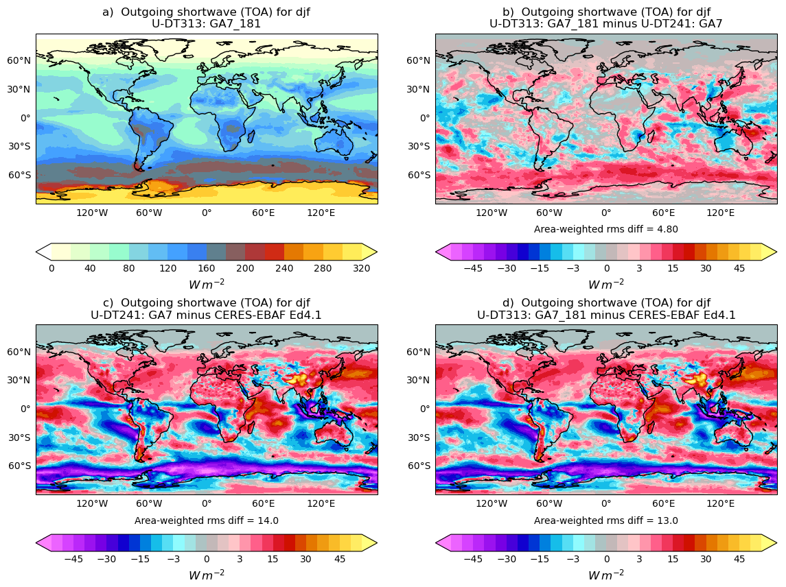
Figure 3 December–February mean top-of-atmosphere outgoing SW radiation (W m⁻²) in the 20 year N96 atmosphere/land only climate simulations compared to Clouds and Earth's Radiant Energy System (CERES) Energy Balanced and Filled (EBAF) dataset version 4.1 (NASA/LARC/SD/ASDC, 2019) showing (a) GA7GL7 with the new parametrisations for riming and depositional growth of ice, (b) the effect of the new parametrisation, (c) bias in GA7GL7 relative to CERES-EBAF and (d) bias in GA7GL7 with the new parametrisation relative to CERES-EBAF.

Convection-permitting modelling shows that these changes improve super-cooled liquid water contents in km-scale simulations of Southern Ocean cyclones (Furtado and Field, 2017). Testing in global simulations also show increases in the liquid water content at mid- and high-latitudes and subsequent reductions in SW flux biases in the Southern Ocean (Fig. 3).

3.4 Boundary layer

3.4.1 Reduce shear-driven entrainment (GMED ticket #172)

The parametrisation of entrainment mixing across the top of convective BLs includes terms from all processes contributing to the production of Turbulent Kinetic Energy (TKE) in the BL. One of these is through shear production and the empirical coefficient in GA7 is set to 5.0, following Driedonks (1982). More recent work (Beare, 2008) has shown that in LES this term is significantly weaker and recommends a value of 1.6. This lower value is used in GA8. The impact of this change is generally small with the most notable difference being a small increase in the amount of marine stratocumulus.

3.4.2 Changes to reduce vertical resolution sensitivity in the BL scheme (GMED ticket #174)

The turbulent mixing and entrainment in cloud-capped BLs is parametrised in terms of (among other things) the strength of cloud-top radiative cooling. This is calculated within the BL scheme by differencing the LW and SW fluxes across the top grid-levels of the cloud layer. The algorithm used prior to GA8 was written when the vertical grids were relatively coarse. Single Column Model (SCM) tests with fine vertical resolution have shown this calculation can still significantly underestimate the change in radiative flux across the top of the cloud when the cooling profile is well resolved (requiring a vertical grid spacing around 50 m or finer). A new methodology identifies where the LW radiative cooling profile transitions from free-tropospheric rates above the cloud to stronger rates within the cloud, and it has been demonstrated in the SCM to be robustly resolution independent down to very fine grids (with approximately 20 m spacing being the finest tested). At standard vertical resolutions the effect of this change is very small.

3.4.3 Turn off BL mixing of ice (GMED ticket #182)

In mixed phase cloud-capped BLs ice particles typically rime supercooled water, grow and fall out of the cloud. In the model, however, there is only a single ice mixing ratio prognostic variable with which to represent the entire size distribution. This results in small ice concentrations having slow fall speeds and so are continuously returned to the cloud layer by turbulent mixing, which leads to further depletion of liquid water. Although a compromise, a better simulation of these clouds is obtained if this mixing is turned off, but limited impacts are seen in other regimes.

3.4.4 Improve the TKE diagnostic and aerosol activation (GMED ticket #197)

An estimate of TKE is calculated by the BL scheme. This is passed to UKCA Activate where it is used to calculate a vertical velocity variance (σ_w) that is used for aerosol activation. The following improvements have been made to this process:

• An indexing error that erroneously shifts the value of TKE upwards by one level when calculating σ_w is fixed. Correcting this error will typically decrease the TKE because TKE usually reduces with height.

• The TKE diagnostic is modified to add an explicit estimate of TKE in convective cloud thereby increasing the overall TKE. TKE is assumed to scale like convective massflux divided by convective cloud area (CCA), based on the assumption that any vertical velocity variance is due to the convective updraught. This change allows UKCA to calculate a direct estimate of σ_w in convective cloud. Note that this change will interact with the revised calculation of CCA described in Sect. 3.5.12.

• The minimum value of σ_w used by UKCA is reduced from 0.1 m s⁻¹, which was often being used to compensate for the lack of representation of TKE within convective cloud, to 0.01 m s⁻¹, which is a more realistic “numerical” minimum.

The combination of these changes tends to reduce TKE which reduces the aerosol activation and cloud droplet number. The cloud droplet effective radius is therefore increased in climate simulations with the largest increases seen in deep convecting regions (Fig. 2c and f). The increase in effective radius is considered to be desirable because the effective radius in GA7 is generally lower than most observation-based estimates (although noting that MODIS, which the model is compared against in Fig. 2, is believed to have a positive bias, e.g. Fu et al., 2022). The increased effective radius darkens the clouds, and the annual mean outgoing SW is reduced by 1.5 W m⁻².

3.4.5 Increase the non-linear solver term for unstable BLs (GMED ticket #290)

The puns parameter controls the BL implicit solver in unstable BLs, specifying an assumed level of non-linearity in the calculation of the diffusion coefficient in the column when the surface buoyancy flux is positive (Wood et al., 2007). Higher values of puns give greater stability but can give excessive damping. As a result, a weak non-linearity value for puns of 0.5 was used prior to GA8, consistent with the non-local nature of the diffusion coefficient calculation in unstable BLs. However, occasional failures have been seen with this setting when there is a column of extremely high winds extending well above the depth of the diagnosed unstable BL depth. The instability is likely generated above the BL where a significantly more non-linear (Richardson-number dependent) diffusion coefficient calculation is used. This hypothesis is supported by the fact that increasing puns to 1.0 greatly reduced the likelihood of this failure mechanism. Additional testing has shown negligible impact on forecast performance, including for example, in the diurnal evolution of the convective BL. For these reasons the value of puns is increased to 1.0 in GA8.

3.4.6 Improved shear-dominated BL diagnosis (GMED ticket #446)

The shear dominated BL type accounts for shear generated turbulence allowing mixing to extend into regions of weak static stability and to potentially inhibit the formation of cumulus. This change modifies the “dynamic diagnosis” of shear driven layers as applied to sea points. In particular, it requires not only that the bulk stability is near neutral (as was the case previously) but also adds the condition that cumulus should have been diagnosed. If these conditions are met, then the surface based mixed layer depth is reset to zero and cumulus diagnosis is set to false. This change addresses a problem identified with the previous “dynamic diagnosis” used in GA7 that it can limit the vertical extent of the surface-based non-local mixing in what should be well-mixed stratocumulus when surface fluxes are small. This change reduces the frequency at which the shear dominated BL type is diagnosed at higher latitudes and reduces cloud in these regions.

3.5 Convection

3.5.1 Improved convection-dynamics coupling (GMED ticket #191)

The convection scheme can sometimes become intermittent in time when the effects of convection on the environment on one timestep can spuriously prevent it being triggered on the next timestep; this is ultimately caused by the time-explicit implementation of the convection diagnosis and closure. Although real convection can be highly variable in time, the intermittency is considered to be unphysical because when averaged over the spatial scales of a model gridbox, real convection does not typically appear and disappear on the timescale of a model timestep. This intermittency is detrimental to the coupling of the convection scheme to the large-scale dynamics, e.g. it can spuriously generate vertically-propagating gravity waves in the lower-stratosphere (although real convection can do this it will be on scales smaller than a model gridbox, and this process is already represented in the model by the non-orographic gravity wave drag scheme as described in Sect. 2.7). To improve the coupling in GA8, time-damped convective increments to potential temperature, θ, and humidity, q, are passed out of the convection scheme rather than instantaneous values. This change is not intended to represent a real physical process but rather to improve the coupling between dynamics and convection, and hence to reduce the effects of the unphysical intermittency. The time-damped increments are defined as:

$$\begin{array}{}\text{(3)}& {\displaystyle \frac{\mathrm{d}{\stackrel{\mathrm{‾}}{S}}_{\mathit{\varphi }}}{\mathrm{d}t}}={\displaystyle \frac{S_{\mathit{\varphi }}-{\stackrel{\mathrm{‾}}{S}}_{\mathit{\varphi }}}{\mathit{\tau }}},\end{array}$$

where ${\stackrel{\mathrm{‾}}{S}}_{\mathit{\varphi }}$ is the time-smoothed increment for ϕ=θ or q, S_ϕ is the instantaneous increment and τ is the damping timescale. This is discretised on timestep n as:

$$\begin{array}{}\text{(4)}& {\stackrel{\mathrm{‾}}{S}}_{\mathit{\varphi }}^n={\displaystyle \frac{\mathrm{\Delta }t}{\mathit{\tau }}}{S}_{\mathit{\varphi }}^n+\left(\mathrm{1}-{\displaystyle \frac{\mathrm{\Delta }t}{\mathit{\tau }}}\right){\stackrel{\mathrm{‾}}{S}}_{\mathit{\varphi }}^{n-\mathrm{1}}\end{array}$$

${\stackrel{\mathrm{‾}}{S}}_{\mathit{\varphi }}^n$ is the smoothed source seen by the rest of the model and is updated each timestep. The damping timescale is not physically constrained but should be as short as possible whilst being long enough to reduce the effects of the intermittency (i.e. ⪆3Δt). It is also desirable that the damping timescale is longer than the Brunt-Vaisala timescale, which is typically 15 min. Given this discussion a damping timescale of 45 min is used at all resolutions. A case could be made for reducing this timescale for higher resolutions (and hence shorter timestep) or for lengthening it for the lowest resolutions, but for the sake of simplicity, ease of implementation and consistency this has not been done. The time-smoothed increments are not advected by the large-scale flow.

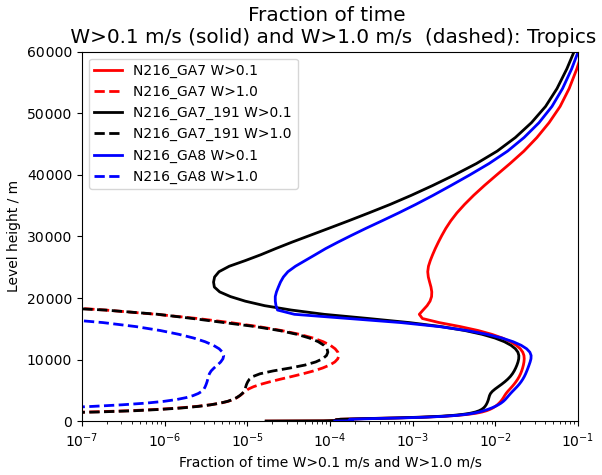
Figure 4 Vertical profile showing the fraction of the time where the vertical velocity exceeds 0.1 m s⁻¹ in solid and 1.0 m s⁻¹ in dashed from 20 year N216 atmosphere/land only climate simulations using GA7GL7 , GA7+#191 and GA8GL9 for 20° S to 20° N.

Time-damping the convective increments greatly reduces the frequency of this spuriously generate vertically propagating gravity waves in the lower-stratosphere as can be seen by the reduction in the frequency of moderately high vertical velocities (>0.1 m s⁻¹) in this region (Fig. 4). This change also helps to reduce the moist bias seen in the lower stratosphere and, importantly, largely removes the resolution dependence of this bias that was seen in GA7.

3.5.2 Improved computational stability in the Gregory-Kershaw type CMT (GMED ticket #198)

Kershaw et al. (2000) investigated the form of the Gregory-Kershaw convective momentum transport (Kershaw and Gregory, 1997; Gregory et al., 1997) used prior to GA8 and showed that not only was it diffusive but also that it was only computationally stable if $\frac{M\mathrm{\Delta }t}{\mathrm{\Delta }p}\le \frac{\mathrm{1}}{\mathrm{1}+c}$ where M is the mass flux, Δp is the pressure thickness of the layer, Δt is the convection timestep and c is positive constant multiplier for the pressure gradient term which accounts for momentum transfer between environment and updraught. Consequently, the limiting Courant number for momentum is less than one whereas for the thermodynamic variables it is one. This feature results in occasional numerical noise in the CMT increments and hence in the wind fields themselves.

Table 4 Discretisation of vertical momentum flux in GA7 (and earlier) and GA8. The modified terms are in bold

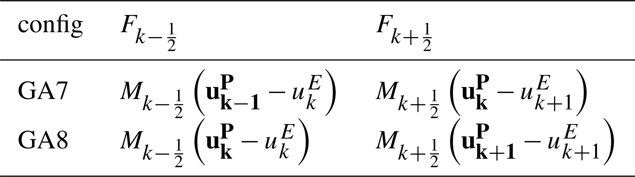
In GA8, the discretisation of vertical momentum flux is modified as shown in Table 4. This changes the condition for computational stability to $\frac{M\mathrm{\Delta }t}{\mathrm{\Delta }p}\le \frac{\mathrm{1}}{\mathrm{1}-c}$ which is guaranteed because the mass flux is limited to be $M\le \frac{\mathrm{\Delta }p}{\mathrm{\Delta }t}$. This change removes the noise that was occasionally seen in the CMT increments, but its wider effects are small.

3.5.3 Prognostic-based convective entrainment rate for deep convection (GMED ticket #199)

The entrainment rate used in a convective parametrisation is an extremely important factor in determining the model's mean climate, its variability and its predictive skill. However, a single entrainment rate is not only unrealistic but can also result in a compromise between the different performance measures. Prior to GA8 once deep convection was diagnosed, fully developed deep convective clouds could instantaneously be generated (within a timestep) without the need for convection to develop and grow because it uses an entrainment rate that is appropriate for fully developed deep convection.

In GA8, we add a simple modification that allows the deep convective entrainment rate to vary over a realistic range of values by linking it to the amount of convective activity within the last several hours, as measured by a 3-dimensional prognostic based on surface convective precipitation, and on the saturated specific humidity at cloud base. Because of the dependence on recent convection, we are adding “memory” into the convection scheme. The underlying premise of the modification is that locations that have experienced high levels of recent convective activity will be populated with relatively large convective clouds that have low entrainment rates: conversely, locations that have experienced low levels of recent activity will be populated with relatively small convective clouds (if any) that will have high entrainment rates. This addition to the convection scheme is briefly described below, and a more detailed description is given in Willett and Whitall (2017).

Memory is introduced into the convection scheme via a new 3-dimensional model prognostic, $\stackrel{\mathrm{‾}}{P}$, that is a measure of recent convective activity:

$$\begin{array}{}\text{(5)}& {\displaystyle \frac{\mathrm{D}\stackrel{\mathrm{‾}}{P}\left(z\right)}{\mathrm{D}t}}={\displaystyle \frac{{\stackrel{\mathrm{̃}}{p}}_{\mathrm{surf}}^{\mathrm{cnv}}-\stackrel{\mathrm{‾}}{P}\left(z\right)}{\mathit{\tau }}}\end{array}$$

where ${\stackrel{\mathrm{̃}}{p}}_{\mathrm{surf}}^{\mathrm{cnv}}$ is a 3-dimensional expansion of the instantaneous 2-dimensional surface convective precipitation rate and is defined as ${\stackrel{\mathrm{̃}}{p}}_{\mathrm{surf}}^{\mathrm{cnv}}=C\left(z\right)max\left[p_{\min },p_{\mathrm{surf}}^{\mathrm{cnv}}\right]$ where the 3-dimensional function, C(z), is set to 1 if convection is active at a given level and 0 if it is not (here, convection is defined as being “active” on any level where the convective temperature tendency, including the contribution from downdraughts/evaporation of precipitation, is non-zero). Non-precipitating convection contributes to $\stackrel{\mathrm{‾}}{P}$ via a small nominal precipitation rate, p_min, which is set to 10⁻⁵ $\mathrm{kg}{\mathrm{m}}^{-\mathrm{2}}{\mathrm{s}}^{-\mathrm{1}}$. $\stackrel{\mathrm{‾}}{P}$ is fully advected with the large-scale flow and, hence, it is very directly coupled to the dynamics. τ, the e-folding time, is set to 3 h (equivalent to a half life of about 2 h) and defines the timescale on which the convective system is expected to have “memory” which is not captured within the resolved fields. This timescale is broadly consistent with previous estimates of the timescales over which convection develops (e.g. Hohenegger and Stevens, 2012) and timescales over which it is expected to have memory (e.g. Davies et al., 2009).

The scaling, F(z), is applied to the entrainment rate such that locations that have had relatively little recent convective activity have higher entrainment rates, and locations that have had high levels of recent convective activity have lower entrainment rates. The scaling is calculated as follows:

$$\begin{array}{}\text{(6)}& F\left(z\right)=C_{\mathrm{grad}}{\log }_{\mathrm{10}}\left(\stackrel{\mathrm{‾}}{P}\left(z\right){\displaystyle \frac{q_{\mathrm{s}}^{\mathrm{ref}}}{q_{\mathrm{s}}^{\mathrm{LCL}}}}\right)+C_{\mathrm{int}},\end{array}$$

where C_grad is a negative constant that determines how strongly the entrainment is related to the prognostic and C_int is an intercept. In GA8, $C_{\mathrm{grad}}=-\mathrm{1.1}$, $C_{\mathrm{int}}=-\mathrm{2.9}$ and the scaling factor F is limited to the range 0.5 to 2.5. $q_{\mathrm{s}}^{\mathrm{LCL}}$ is the saturated specific humidity at the Lifting Condensation Level (LCL), and the reference value for normalisation is $q_{\mathrm{s}}^{\mathrm{ref}}=\mathrm{20.0}$ g kg⁻¹. The dependence on $q_{\mathrm{s}}^{\mathrm{LCL}}$ accounts for the fact that temperature exhibits a strong control on precipitation rates; without this dependence Eq. (6) would always diagnose very high entrainment rates in mid-latitude or high-latitude conditions. Note that the scaling has a logarithmic dependence on $\stackrel{\mathrm{‾}}{P}$; this reflects the fact that precipitation rates can vary over several orders of magnitude, but it is required that the scaling should only vary by a factor of ∼5. The values of C_grad and C_int used in Eq. (6) were arrived at by using estimates of the range of tropical precipitation rates (from 3-hourly TRMM and model data) and associated entrainment rates (the lower limit being approximately half the current value used in deep convection and the upper limit being similar to values used by the shallow convection scheme). Values of F for a range of values of $\stackrel{\mathrm{‾}}{P}$ and $q_{\mathrm{s}}^{\mathrm{LCL}}$ are shown in Table 5. It should be noted that the precipitation rates used here represent averages over the timescale τ=3 h, and over a global model grid-box Δx ∼ 10–100 km and hence they are considerably smaller than the expected instantaneous local precipitation rates occurring within convective cells.

Table 5 Table of entrainment rate scaling F as function of $\stackrel{\mathrm{‾}}{P}$ and saturated humidity values at the LCL of 5 and 20 g kg⁻¹ at the LCL. The values in brackets indicate the value of F before the minimum and maximum limits have been applied.

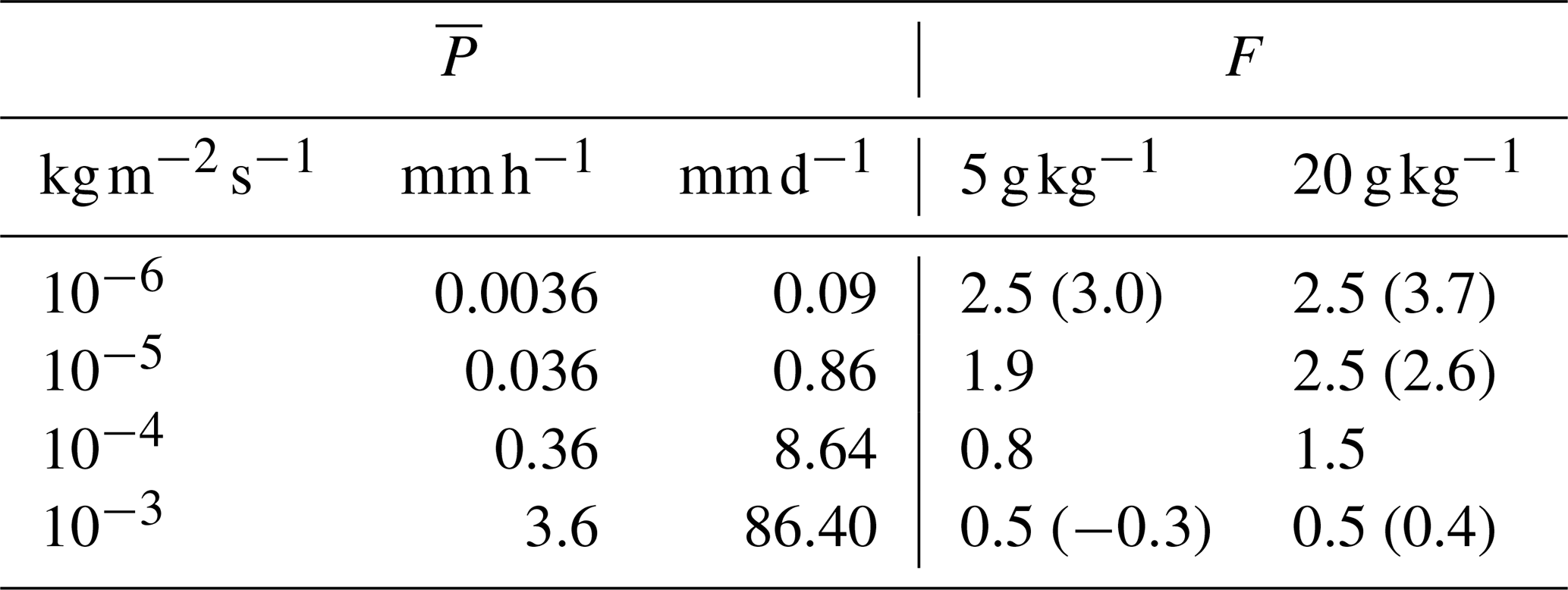
The factor, F, is used to scale the standard deep convection entrainment rate profile, i.e.:

$$\begin{array}{}\text{(7)}& \mathit{ϵ}\left(z\right)=F\left(z\right)f_{dp}\mathrm{4.5}g{\displaystyle \frac{\mathit{\rho }\left(z\right)p\left(z\right)}{P_{\mathrm{0}}^{\mathrm{2}}}}\end{array}$$

where p is pressure, p₀ is the pressure at the surface and ρ is density. The profile is identical to that originally used in Gregory and Rowntree (1990) apart from the prognostic-based scaling factor F and the additional tuning parameter f_dp that is set to 1.0 in GA8 because the use of F makes it redundant. Note that in the convection scheme, the fractional entrainment rate ϵ is computed in pressure vertical coordinates (units Pa⁻¹), and the factor gρ has been added in Eq. (7) to convert the units to m⁻¹.

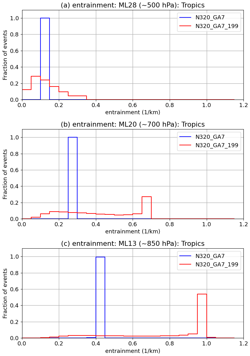
Figure 5 Histogram of entrainment rate for deep convection (km⁻¹) in the tropics (20° S to 20° N) at model levels (a) 28 (∼ 5.6 km/500 hPa), (b) 20 (∼ 2.9 km/700 hPa) and (c) 13 (∼ 1.3 km/850 hPa) for GA7GL7 and GA7GL7 with ProgEnt from a 5 d N320 case study. The entrainment rate was sampled hourly. To facilitate the production of the entrainment diagnostic, only a single convective substep was used in the model runs.

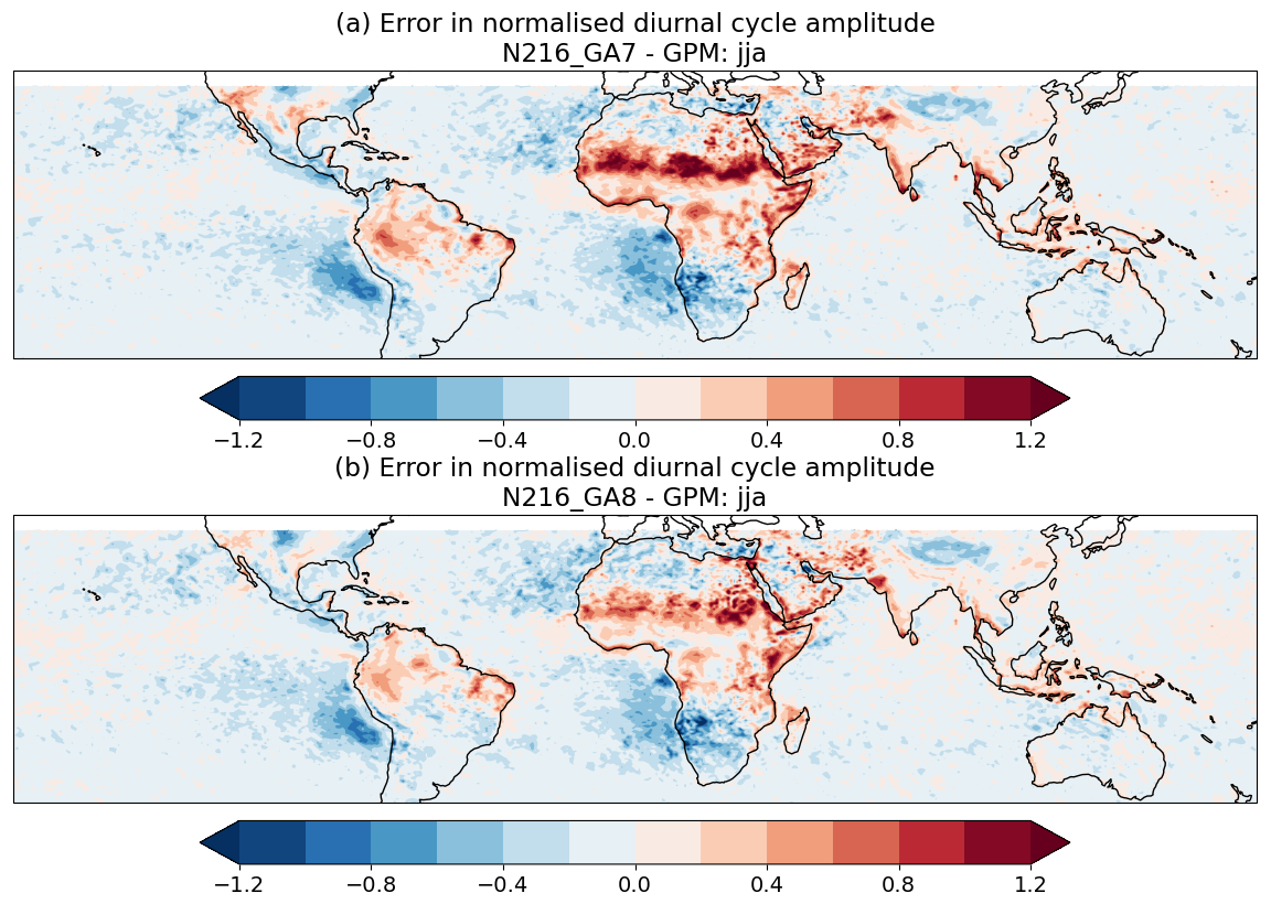
Figure 6 Error in normalised amplitude of the seasonal mean diurnal cycle for (a) GA7GL7 and (b) GA8GL9 relative to GPM for JJA. The season mean diurnal cycles from the model configurations are aggregated using 20 years of 3-hourly instantaneous precipitation rates. The seasonal mean diurnal cycle for GPM IMERG (Huffman et al., 2020a, b) was aggregated from 10 years of 3-hourly instantaneous precipitation rates and regridded to the model grid using area-averaged weighting. The normalised amplitude is calculated by dividing the standard deviation of the mean diurnal cycle by its mean (i.e. the coefficient of variation of the seasonal mean diurnal cycle).

Figure 5 shows histograms of the entrainment rate for deep convection from 5 d N320 simulations for a selection of model levels that approximately equate to 850, 700 and 500 hPa. GA7 essentially has a single entrainment rate at each height. The addition of the prognostic-based entrainment allows deep convection to use a much wider range of entrainment rates and can represent convection at different states of development. At any given moment, deep convection will be initiating at many locations where has been little or no recent convective activity. In this situation, GA7 will use its single fixed entrainment profile which is suitable for fully developed deep convection; ProgEnt, however, will use its highest entrainment rate (hence the peak in the 850 hPa histogram) suitable for developing convection. At higher heights, the distribution of entrainment rates seen with ProgEnt shifts towards the lower end of its available range as the higher entrainment events are preferentially terminated at lower levels. The range of entrainment rates available with ProgEnt is consistent with those derived in high resolution simulations especially at low-levels. For example, at ∼ 1.3 km/850 hPa ProgEnt has a range of approximately 0.2 to 1.0 km⁻¹ which compares well with values of 0.3 to 1.3 km⁻¹ shown in Stirling and Stratton (2011) and 0.2 to 0.7 km⁻¹ shown in de Rooy et al. (2013).

The most important impact of ProgEnt is that it improves the instantaneous structure of convection and consequently improves the structure of associated fields such as precipitation, cloud condensate, outgoing LW and SW radiation, etc.; this is discussed further in Sect. 4.2. In isolation, ProgEnt improves the phase of diurnal cycle of precipitation; however, other changes included in GA8 (mainly the improved convection-dynamics coupling – Sect. 3.5.1) offset much of the improvement in the phase (Table 6). ProgEnt does help to reduce the excessive amplitude in the diurnal cycle, which is seen in regions such as the Sahel in the control, and this benefit is maintained in GA8 (Fig. 6). When added to GA7 without any further modification, ProgEnt does increase the biases in tropical temperatures, but this is addressed through tuning as discussed in Sect. 3.9.

Table 6 Median absolute phase error in hours in the seasonal-mean diurnal-harmonic for land points between 40° S and 40° N for N96 GA7GL7, GA7GL7+ProgEnt and GA8GL9 configurations relative to GPM IMERG V06B (Huffman et al., 2020a, b). The seasonal mean diurnal cycles from the model configurations are aggregated using 20 years of 3-hourly instantaneous precipitation rates. The seasonal mean diurnal cycle for GPM IMERG was aggregated from 10 years of 3-hourly instantaneous precipitation rates and regridded to the model grid using area-averaged weighting. The values in brackets are differences from the GA7GL7 values.

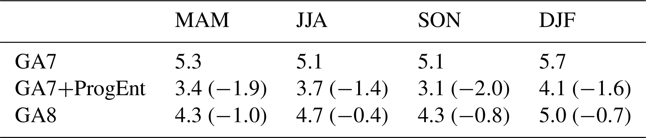
3.5.4 Melt convective snowfall in the downdraught/environmental air over more than one level (GMED ticket #205)

Prior to GA8, snow generated within the convection scheme melts within a single level when it reached the melting level. This process resulted in a spike in the temperature increments from the convection scheme at the melting level. The magnitude of this spike increases with vertical resolution as the layer over which the melting occurs becomes thinner. This change replaces the instantaneous melting of snow with snow melting over a characteristic temperature thickness and at a rate proportional to the temperature above the melting level. For snow falling in the environment we have:

$$\begin{array}{}\text{(8)}& {\displaystyle \frac{\mathrm{dSNOW}}{\mathrm{d}{T}^{\mathrm{E}}}}=-{\displaystyle \frac{\left(T^{\mathrm{E}}-T_{\mathrm{melt}}\right)\mathrm{SNOW}}{\mathrm{\Delta }{T}_{\mathrm{melt}}^{\mathrm{2}}}}\end{array}$$

where T^E is the temperature of environment, T_melt is the melting level (set to 273.15 K) and ΔT_melt defines a characteristic temperature thickness over which the melting occurs and is set to 3 K. The same melting scheme is applied to snow falling within the downdraughts, but with the temperature of the environment replaced by the temperature of the downdraught. Furthermore, convective rainfall is now permitted to freeze but this is described in Sect. 3.5.11.

3.5.5 Revised forced detrainment calculation (GMED ticket #207)

Forced adaptive detrainment is a mechanism within the convection scheme that represents an ensemble of plumes with a range of buoyancies whilst only explicitly calculating the mean buoyancy (Derbyshire et al., 2011). It preferentially detrains the part of the distribution that is no longer buoyant and thereby increases the buoyancy of the remaining parcel albeit at the expense of reduced mass flux. In previous configurations, when the air within convective updraught became unsaturated and forced detrainment was triggered, the humidity of the parcel undergoing forced detrainment was assumed to have the parcel mean humidity. The forced detrainment was, consequently, unable to modify the humidity of the remaining parcel and it would remain unsaturated. This usually results in the updraught terminating as soon as it becomes unsaturated even though convection may still have been viable for some fraction of the distribution.

This change improves the treatment of subsaturated forced detrainment by assuming the detrained parcel has a humidity equal to that of the mean of the environment and parcel humidities. This allows subsaturated force detrainment to increase the humidity of the remaining parcel and hence increases the likelihood of convection continuing. The effect of this change is to allow convection to become slightly deeper. This ultimately results in a warming of ∼0.1 K at around 600 and 100 hPa, and a ∼0.1 K cooling at around 250 hPa.

3.5.6 Additional termination condition for convection (GMED ticket #417)

Prior to GA8, the convective parcel ascent terminates when one of the following conditions is met: the mass flux falls below a small fraction (5 %) of cloud base mass flux; the forced detrainment needs to detrain a large fraction (95 %) of the mass flux; or the parcel approaches the top of the model (although this final condition will only ever be triggered if a numerical instability is encountered).

However, the combination of the low entrainment rates available with the prognostic-based entrainment (Sect. 3.5.3) and adaptive forced detrainment mean that the height reached by the convective parcel ascent can occasionally exceed that of an undilute (i.e. zero entrainment) parcel. This is unphysical (especially since we do not expect or want the scheme to represent overshooting) because an undilute parcel denotes the upper limit of possible buoyancies and could be considered to represent a protected core that does not entrain any environmental air. To address this issue the convection scheme now performs an undilute (zero entrainment) parcel ascent in parallel with the main dilute ascent. In addition to the conditions listed above, the main dilute parcel will now terminate when it reaches the level of neutral buoyancy of the undilute parcel ascent. This change helps to reduce the high humidity bias in the lower stratosphere because it prevents spuriously overshooting convection detraining water into the lower stratosphere.

3.5.7 Use real surface fluxes in the convection diagnosis (GMED ticket #431)

The convection diagnosis uses the surface fluxes to determine if the surface is unstable or not and in the calculation of a buoyancy excess that is used in a adiabatic parcel ascent. This parcel ascent provides an initial estimate of BL height and determines whether or not shallow or deep convection should be triggered.

Prior to GA8, a simplified estimate of surface fluxes was used within the convection diagnosis compared to the full calculation done within JULES. In GA8, JULES is called before the convection diagnosis so that the diagnosis can use the “real” explicit estimate of surface fluxes from JULES. This change has only a very small impact but does improve the self-consistency of the model.

3.5.8 Switch off the convective water and energy correction (GMED ticket #474)

The 6a convection scheme, which was added in GA7 (Walters et al., 2019, Sect. 3.7.1), includes a correction to the water and energy that was not included in the previous version of convection scheme. Even without the correction, the water and energy conservation in the 6a scheme is very good, but small errors can be generated because it assumes hydrostatic balance and a shallow atmosphere (it uses pressure levels) whilst the model dynamics is non-hydrostatic and assumes a deep atmosphere. This correction step, however, tends to produce a small (∼0.1 K) tropospheric warming that results in a negative impact on verification scores. For that reason, the correction is pragmatically switched off in GA8. The overall conservation of energy and water in the model is no worse with this correction switched off. This is probably because it introduces a small compensating error that offsets other sources of non-conservation within the model.

3.5.9 Limit CAPE timescale to reduce convectively coupled waves (GMED ticket #476)

GA7 introduced a CAPE timescale that is dependent on the large-scale vertical velocity (Walters et al., 2019, Sect. 3.7.2). Larger vertical velocities result in shorter CAPE timescales with the lower limit being the convection timestep which is half the model timestep. This results in the lower limit of CAPE timescale being extremely short at higher horizontal resolutions with their shorter timesteps. For example, at N1280 the minimum CAPE timescale would be just 2 min. However, it was noted that at higher resolutions this closure increases the frequency of spurious fast-moving, convectively coupled waves. This issue is greatly mitigated in GA8 by simply limiting the minimum CAPE timescale to 30 min.

3.5.10 Gregory-Kershaw CMT for deep convection and associated tuning (GMED ticket #487)

Previous configurations used the turbulent CMT for deep convection and Gregory-Kershaw (GK) CMT for mid-level convection. The turbulent CMT used in deep convection has little justification other than an extrapolation from the shallow turbulent CMT. Furthermore, it is difficult to justify using different schemes for deep and mid-level convection. For these reasons GA8 uses the stabilised Gregory-Kershaw scheme (Sect. 3.5.2) in both deep convection and mid-level convection. When switching from turbulence to GK CMT the effect of the CMT is reduced; furthermore, the increased entrainment rates available with prognostic based entrainment (Sect. 3.5.3) can pull the parcel winds closer to those of the environment and also act to the reduce the effect of the CMT. To compensate for this, the parameter controlling the pressure gradient term in the GK CMT, cpress_term, is reduced in GA8 which acts to increase the effect of the GK CMT and bring it closer to the level seen in GA7.

3.5.11 Allow freezing of convective rain (GMED ticket #528)

Condensed water within the convective parcel is assumed to form as liquid above −10 °C and as ice at lower temperatures. The phase of the condensed water is retained upon autoconversion to precipitation and hence convective precipitation forms as liquid down to −10 °C. However, prior to GA8 falling convective precipitation was assumed to freeze instantly when it encountered temperatures below 0 °C, and consequently rain created below 0 °C instantly freezes over a single model level. This could potentially lead to unphysically sharp features in the temperature increments from convection and to excessive sensitivity to the vertical resolution of the model. This change replaces the instantaneous freezing of rainfall with rainfall freezing over a characteristic temperature thickness and at a rate proportional to the temperature below the freezing level (in a functionally similar manner to the melting of snow in Sect. 3.5.4). For rain falling in the environment, we have:

$$\begin{array}{}\text{(9)}& {\displaystyle \frac{\mathrm{dRAIN}}{\mathrm{d}{T}^{\mathrm{E}}}}=-{\displaystyle \frac{\left(T_{\mathrm{melt}}-T^{\mathrm{E}}\right)\mathrm{RAIN}}{\mathrm{\Delta }{T}_{\mathrm{melt}}^{\mathrm{2}}}}\end{array}$$

where the symbols have the same meaning as in Eq. (8). The same freezing scheme is applied to rain falling within the downdraughts but with the temperature of the environment replaced by the temperature of the downdraught. The impact of this change is small, but it reduces the sensitivity of the representation of this process to the vertical resolution of the model and is scientifically consistent with the treatment of convective snowfall as described in Sect. 3.5.4.

3.5.12 Convective cloud amount from mass flux equation (GMED ticket #529)

Prior to GA8, CCA for deep and mid-level convection uses a formulation based on logarithm of surface convective precipitation which is difficult to justify. Furthermore, since CCA does not scale linearly with mass flux the time-averaged CCA becomes dependent on the level of intermittency and hence convective closure which is undesirable.

In GA8, the CCA is derived directly from a depth-averaged mass flux and an assumed in-cloud vertical velocity. This formulation is more consistent with the CCA calculation for shallow convection. The cloud fraction is derived from the mass flux equation, M=CCA ρ w_cnv where ρ if the air density and w_cnv is vertical velocity of the convective parcel. Since we only require a 2-dimensional CCA, CCA2d, we use the vertically mass-weighted measure, $\stackrel{\mathrm{‾}}{\left(\frac{M}{\mathit{\rho }}\right)}$, where the overbar indicates a mass weighted vertical average. CCA2d is then calculated as:

$$\begin{array}{}\text{(10)}& \mathrm{CCA}\mathrm{2}\mathrm{d}={\displaystyle \frac{\mathrm{1}}{w_{\mathrm{cnv}}}}\stackrel{\mathrm{‾}}{\left({\displaystyle \frac{M}{\mathit{\rho }}}\right)}\end{array}$$

where w_cnv is assumed to be 1 m s⁻¹ which is consistent with observational estimates. This new formulation necessitated retuning of the scalings that are applied to CCA2d before it is passed to the radiation scheme which is discussed in Sect. 3.9. A desirable outcome of the this change is that the scalings are now much closer to one.

3.6 Aerosols

3.6.1 Black Carbon and aerosol absorption updates (GMED ticket #257)

Following Mulcahy et al. (2018), the refractive index of Black Carbon (BC) aerosol in RADAER is updated from the value in WCP 1983 to the middle estimate provided by Bond and Bergstrom (2006), i.e. from 1.75 + 0.44 i to 1.85 + 0.71 i at 550 nm. This increases SW absorption by the BC component by approximately 60 %. The resolution of refractive index imaginary part (RIimag) in the RADAER look-up-tables is increased so that small values of RIimag can be resolved. This increases absorption in regions where the mass fraction of BC in the aerosol is small (e.g. <1 %) and the absorption may have previously been unrepresented. Mulcahy et al. (2018) demonstrated that in GA7.1 this update to BC properties greatly reduced the low bias in absorption aerosol optical depth relative to AERONET (Aerosol Robotic Network) observations.

3.6.2 Upgrade source for dimethylsulfide (DMS) seawater concentration (GMED ticket #272)

The DMS seawater concentration ancillary has been updated to the more recent Lana et al. (2011) climatology. This new dataset is derived from a much larger number of observations than its predecessor (Kettle et al., 1999), and improved statistical interpolation and extrapolation techniques were also employed in generating a global gridded dataset from discrete ship-based observations. This update results in a 12 % global annual mean increase in marine DMS emissions from 34.5 to 38.7 Tg[S] yr⁻¹ and subsequent increases in aerosol optical depth and cloud droplet number concentrations, increase the net outgoing SW radiation at the top-of-atmosphere by approximately 0.2 W m⁻².

3.6.3 Implement a representation of marine organic aerosol (GMED ticket #277)

GLOMAP-mode, which was added in GA7 (Walters et al., 2019, Sect. 3.8), included a representation of primary marine organic sources of aerosol. However, in GA7.1 it was found necessary to scale the marine DMS emissions by 1.7 to account for missing primary marine organic sources (PMOA) of aerosol in the model (Mulcahy et al., 2018). A new primary marine organic aerosol emission parametrisation was subsequently developed and implemented into UKESM1.0 (Mulcahy et al., 2020). In GA8 we adopt this new parametrisation. The scheme and its implementation are described in detail in Mulcahy et al. (2020), but we provide a brief description here for completeness.

This emission parametrisation follows that of Gantt et al. (2011) with updates from Gantt et al. (2012), where the organic fraction of the underlying sea spray is calculated as:

$$\begin{array}{}\text{(11)}& \begin{array}{rl}{\mathrm{OM}}_{\mathrm{SSA}}& ={\displaystyle \frac{\frac{\mathrm{1}}{\mathrm{1}+\exp \left(\mathrm{3}\left(-\mathrm{2.63}\mathrm{Chl}\right)+\mathrm{3}\left(\mathrm{0.18}{U}_{\mathrm{10}}\right)\right)}}{\mathrm{1}+\mathrm{0.03}\exp \left(\mathrm{6.81}{D}_p\right)}}\\ & +{\displaystyle \frac{\mathrm{0.03}}{\mathrm{1}+\exp \left(\mathrm{3}\left(-\mathrm{2.63}\mathrm{Chl}\right)+\mathrm{3}\left(\mathrm{0.18}{U}_{\mathrm{10}}\right)\right)}}\end{array}\end{array}$$

Where Chl is the surface chlorophyll concentration, U₁₀ is the 10 m windspeed and D_p is the sea salt dry diameter. While in UKESM1.0 the chlorophyll fields are provided for by the ocean biogeochemistry model, here we use the Globcolour Chlorophyll dataset (Ford et al., 2012). The emissions of PMOA are then calculated as:

$$\begin{array}{}\text{(12)}& E_{\mathrm{PMOA}}=V_{\mathrm{SS}}{\mathrm{OM}}_{\mathrm{SSA}}{\mathit{\rho }}_{\mathrm{SSA}}\end{array}$$

Where V_SS is the volume emitted flux of sea salt and ρ_SSA is the apparent density of emitted sea spray aerosol given by:

$$\begin{array}{}\text{(13)}& {\mathit{\rho }}_{\mathrm{SSA}}={\mathrm{OM}}_{\mathrm{SSA}}{\mathit{\rho }}_{\mathrm{OM}}+\left(\mathrm{1}-{\mathrm{OM}}_{\mathrm{SSA}}\right){\mathit{\rho }}_{\mathrm{salt}}\end{array}$$

Where ρ_OM and ρ_salt are the densities of organic matter (1500 kg m⁻³) and sea salt (2165 kg m⁻³) respectively. Gantt et al. (2012) applied a global scaling factor of 6 to the diagnosed emissions above. However, following Mulcahy et al. (2020), who found that the global emissions of PMOA in UKESM1 compared well with Gantt et al. (2012) without the scaling, we do not apply the scaling here. Similarly, we do not include the scaling that was applied to the marine DMS emission in GA7.1 as an oversimplified representation of missing marine emission sources (Mulcahy et al., 2018).

3.6.4 Update source for UKCA 3D volcanic SO2 emissions (GMED ticket #363)

The volcanic SO₂ emission input data that represents the continual degassing from volcanoes into the troposphere (rather than explosive injection into the stratosphere as discussed in Sect. 2.10) is updated from the older dataset of Andres and Kasgnoc (1998) to the newer dataset of Dentener et al. (2006), as provided for the Aerocom model intercomparison. The data sources are the same for both, but they are subject to differing processing which alters the horizontal and vertical distribution of emissions (see Dentener et al., 2006, for details). Additionally, an error was discovered in our use of the older data that resulted in erroneously large emissions. The combined impact of these changes was to reduce global total volcanic SO₂ emissions by a factor of approximately two to 28.8 Tg yr⁻¹.

3.7 Dynamical formulation and discretisation

3.7.1 Multigrid solver (GMED ticket #531)

As described in Sect. 2.2, the UM uses a nested iterative structure for each timestep which is split into inner and outer loops. At the end of the inner-loop it is necessary to solve the Helmholtz problem for the pressure increment. In GA8, a new multigrid solver is used in the Helmholtz solver.

Multigrid (for an introduction see e.g. Wesseling, 1995) is an iterative numerical technique for the efficient solution of the system of sparse linear equations that arises in semi-Lagrangian timestepping. By using a series of coarser and coarser numerical grids, the solution to the discretised equations can be found while performing much less computational work and by passing much less information between processors (Buckeridge and Scheichl, 2010; Müller and Scheichl, 2014). These attributes mean that for most cases multigrid is faster than the postconditioned variant of van der Vorst's bi-conjugate gradient stabilized (BiCGstab) method (van der Vorst, 1992) used in GA7. Since the solver is independent of the system of equations that is to be solved and all iterative schemes reduce the numerical error below a pre-defined tolerance, this change does not represent a fundamental difference in physical representation: both the multigrid solver and the existing method produce a solution of the sparse linear system within the specified accuracy. The multigrid scheme has only a small impact on overall forecast performance in most circumstances but does produce noticeably smoother solutions at the poles.

3.8 Corrections

3.8.1 Correction to exchange coefficient in dust deposition (GMED ticket #173)

This change fixes a bug in the calculation of the surface layer friction velocity, U^∗, where it appears in the calculation of surface layer resistance for surface deposition of dust. The impact is to generate a larger exchange coefficient for surface deposition leading to a small reduction in low level dust concentration.

3.8.2 Correct evaporation of convective precipitation (GMED ticket #208)

Convective precipitation is allowed to evaporate in the downdraught and in the subcloud layer. The rate of evaporation depends on the local precipitation rate. For evaporation in the subcloud layer the local precipitation rate is defined by $P_{\mathrm{local}}=\frac{P}{\mathrm{CCA}}$ where P is the gridbox mean precipitation rate due to the updraught and CCA is the fraction of the gridbox occupied by the updraught. The local precipitation for the downdraught is calculated in a similar manner but uses the gridbox mean downdraught precipitation and the fraction of the gridbox occupied by the downdraught. A bug was identified whereby the CCA was double counted, and this change corrects this error. The local precipitation rate will be reduced by this fix and hence the evaporation rate will increase. The overall impact of this fix, however, is very small.

3.8.3 Correction to shear-dominated BL type (GMED ticket #269)

The diagnosis of BL regime was originally based almost entirely on the state of the thermodynamic and moisture profiles of the lower atmosphere. The diagnosis took little account of the generation of mixing through wind shear influencing the regime, and, in particular, disrupting the diagnosis of cumulus convection. An initial test monitored $-z_h/L$ (z_h = BL depth and L = Obhukov length and so gives a measure of the stability of the surface layer) and when this came close to neutral the cumulus flag was reset to false and the mixed layer depth set to zero, leaving the local Richardson (Ri) number-based BL scheme to generate any mixing. Following studies of cold-air outbreaks, a second rediagnosis was added that considered how far shear-driven turbulence (given by the Ri-based diagnosis of BL depth, z_h(Ri)) would penetrate into a cumulus cloud layer. If it crossed a threshold fraction of the cloud layer depth, the cumulus flag would again be reset to false, but this time the mixed-layer depth would be reset to the diagnosis parcel top, on the assumption that wind shear would disrupt cumulus formation and allow quasi-homogeneous turbulence to maintain a well-mixed layer to that depth. Unfortunately, the two diagnoses were combined such that even in the case that $-z_h/L$ was close to neutral, the mixed layer depth would incorrectly be set to the diagnosis parcel top. The correction here is to separate these two changes to be as originally intended – i.e $-z_h/L$ close to neutral gives zero mixed layer depth and z_h(Ri) sufficiently high into the cloud layer gives the mixed layer depth equal to the diagnosis parcel top height. The z_h(Ri) test is performed preferentially so as to allow well-mixed layers identified by that method to be maintained even when $-z_h/L$ is close to neutral. The effect of this correction is very small.

3.8.4 Correction to BL depth prognostic with forced cumulus (GMED ticket #301)

The forced cumulus option, first used in GA7 and described in Walters et al. (2019), erroneously sets the prognostic BL depth variable, z_h, to just the non-local layer depth rather than the maximum of local and non-local depths. This results in the BL depth diagnostic erroneously being overwritten with this non-local depth (which is zero at night, for example). It also leads to errors in the actual model evolution because z_h is used elsewhere in the implicit BL and on the next timestep in the convection diagnosis. This change corrects this error and consequently replaces the non-local BL depth with the physical BL depth in the calculation of BL frictional heating, the BL velocity scale, surface layer depth and maximum buoyancy perturbation in the convection diagnosis as well as in the BL depth diagnostics. In practice, only the change to frictional heating has a non-negligible effect on model evolution.

3.8.5 Fix water conservation in PC2 ice/water partition in convection (GMED ticket #434)

PC2 retrospectively re-partitions the phase of the original forced detrainment increments for liquid and frozen water within the convection scheme. In GA7, this process assumes that the convective parcel cannot have mixed phase. This is only true, however, above the initiation level because at cloud base the convective parcel is initialised with environmental liquid and frozen water, and both phases can co-exist within the environment. Therefore, if the initial level has mixed phase and there is forced detrainment between the initial level and the level above, the scheme will not exactly conserve water (although the error is typically very small). This change corrects the logic within the scheme to allow for mixed phased condensate within PC2's re-partition of the forced detrainment increments of liquid and frozen water. Although this change substantially improves the conservation of water, it has a negligible effect on the model's performance.

3.8.6 Other minor bug fixes (GMED ticket #484)

In the UM “temporary logicals” are used to protect fixes to the UM that significantly alter science configurations. The protection is provided so that a defined GA/GL/GC configuration is scientifically consistent across a limited number of UM releases. From a technical perspective, we wish to set as many temporary logicals to true at each GA configuration because this will aid the retirement of the logicals and simplify the code. From a scientific perspective, we wish to set them to true because that will fix bugs in the code and enhance the scientific integrity of the model. For GA8GL9, all available temporary logicals available at the time of the freeze (i.e. those that existed in UM vn11.4) were set to true. The list of fixes applied including a brief description is given in Table 7.

Table 7 Temporary logicals set to true as part of #484.

Most of these corrections have a negligible effect on the model evolution or on the model's climate and some have zero effect in some applications. Overall, the most notable effect of these changes is to increase the clear-sky outgoing SW radiation by about 0.2 W m⁻² which is mostly due to the change in sea-salt density.

3.9 Tuning

Tuning is an essential and unavoidable part of the model development process that has received increasing attention over recent years (e.g. Schmidt et al., 2017; Hourdin et al., 2017), and the need to document this process has been widely recognised. Tuning is needed to ensure that biases are minimised and that the overall scientific performance reaches an acceptable level across a wide range of measures and experiment types. As a general principle when developing GA/GL configurations, the aim is to deliver a configuration that is at least as good as its predecessor overall and that does not significantly degrade the representation of any key process, and tuning helps to deliver this.

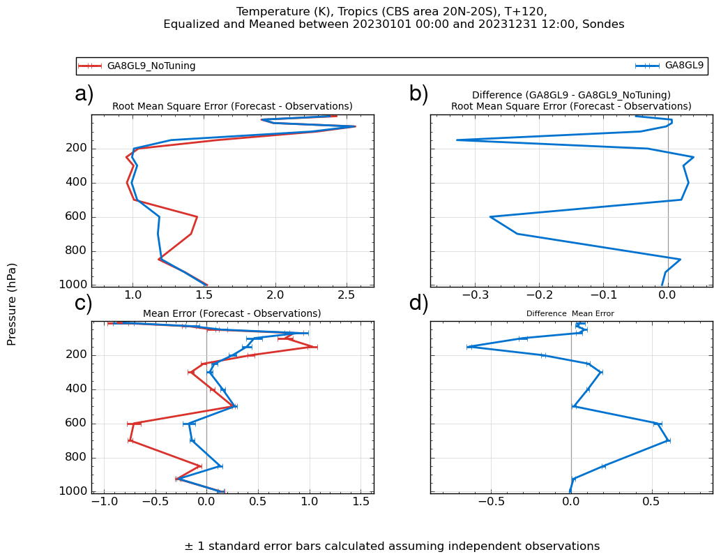
Figure 7 Verification with respect to sondes of tropical T + 120 temperatures forecasts from N320 GA8 without tunings and standard GA8 showing (a) RMSE, (b) difference in RMSE, (c) mean error, and (d) difference in mean error for 59 cases between January and December 2023.

Each change included in GA8GL9 was tested individually using present day N96 AMIP simulations, N320 NWP case studies and, for some larger changes, N320 Data Assimilation (DA) trials. All the changes from each science area (e.g. BL, convection etc) were packaged together and tested again using N96 AMIP simulations, N320 NWP case studies and DA trials. The science area packages were then incrementally added together and tested. Throughout this process model deficiencies were identified and recorded. Any changes in bias or model behaviour are therefore traceable to individual changes or combinations of changes. This helps in identifying the physical mechanism for errors introduced during the development process and hence helps to identify potential mitigation measures. Possible mitigation measures could include the introduction of an additional science change (both the time-smoothed convection increments in Sect. 3.5.1 and the additional convective termination condition in Sect. 3.5.6 are examples for GA8GL9), by the tuning of some model parameters as discussed in this section, or by not including a change in the configuration if the error it introduces cannot be addressed (this was not done for GA8GL9). As a general principle, the values for the parameters are only tuned within the estimation of their uncertainty.

There are a very large number of tuneable parameters in the model, and it is clearly impractical to test the sensitivity to each of these in the model development process. A far smaller number of parameters that may affect an error can be identified by considering the following: the effect of individual science changes on the error, a physical understanding of the processes leading to the error, an understanding of what parameters do within a physics scheme and the likely effects of changing their value, and results from previous parameter sensitivity tests (possibly at earlier configurations). Throughout the development of GA8GL9 these considerations were used to identify parameters that may be used to reduce any new errors, and the sensitivity to these parameters was usually tested using present day N96 AMIP simulations and N320 NWP case studies.

At the Met Office at the time of the development of GA8GL9, it was planned to replace GA7.2GL8.1 (Willett et al., 2023) with GA8GL9 in its coupled form, GC4, as the operational global NWP model. It was therefore considered essential that GA8GL9 should at least match GA7.2GL8.1 in terms of NWP performance. The tropical temperature biases seen in GA7GL7 were one of the main reasons why it was not considered acceptable for operational NWP. Consequently, a major focus of the development and tuning GA8GL9 was the reduction of tropical temperature biases seen in GA7GL7. In many applications GA8GL9 will be coupled to ocean and sea-ice models as GC4, and it was therefore considered important that the global mean net top of atmosphere (TOA) radiative flux is close to observed estimates to avoid any spurious long-term drifts in the ocean or the sea-ice. So that the constraint on the net TOA is obtained in a physically realistic manner, it was also required that the global mean SW and LW TOA radiative fluxes were close to observed values whilst avoiding large increases in regional biases in these fluxes. The primary aims of the tuning process were, therefore, to reduce tropical temperature bias and to constrain the TOA radiative fluxes within acceptable limits: the selection of tuning parameters and their values was largely determined by these aims. It should be stressed, however, that we wished to achieve these primary aims whilst avoiding any degradation in (and ideally improving upon) the wider scientific performance of the model. It should be noted that these constraints on tropical temperature and radiative fluxes are not independent because tropical cloud, which is predominantly generated in the convection scheme, affects both the tropical temperature structure and radiative fluxes.

Table 8 Global- and annual-mean fluxes from 20 year N96 AMIP simulations using GA8GL9 without the tunings in Table 9 and standard GA8GL9 with the tunings, and observed estimates. The observed estimates of radiative fluxes are from CERES-EBAF edition 4.0 (Loeb et al., 2018) and the precipitation from GPCP version 3.2 (Huffman et al., 2023).

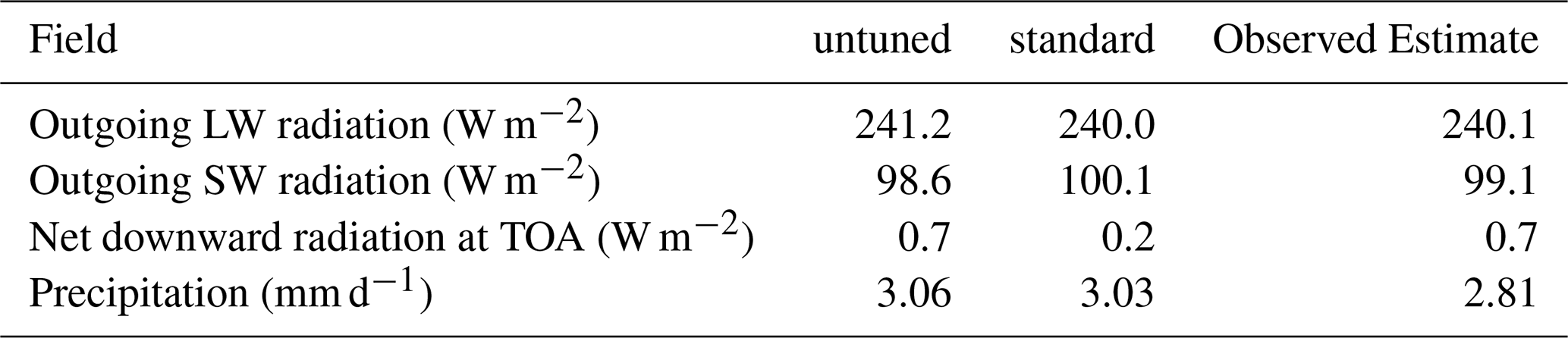
Table 9 Initial proposed and final values of parameters tuned in GA8GL9.

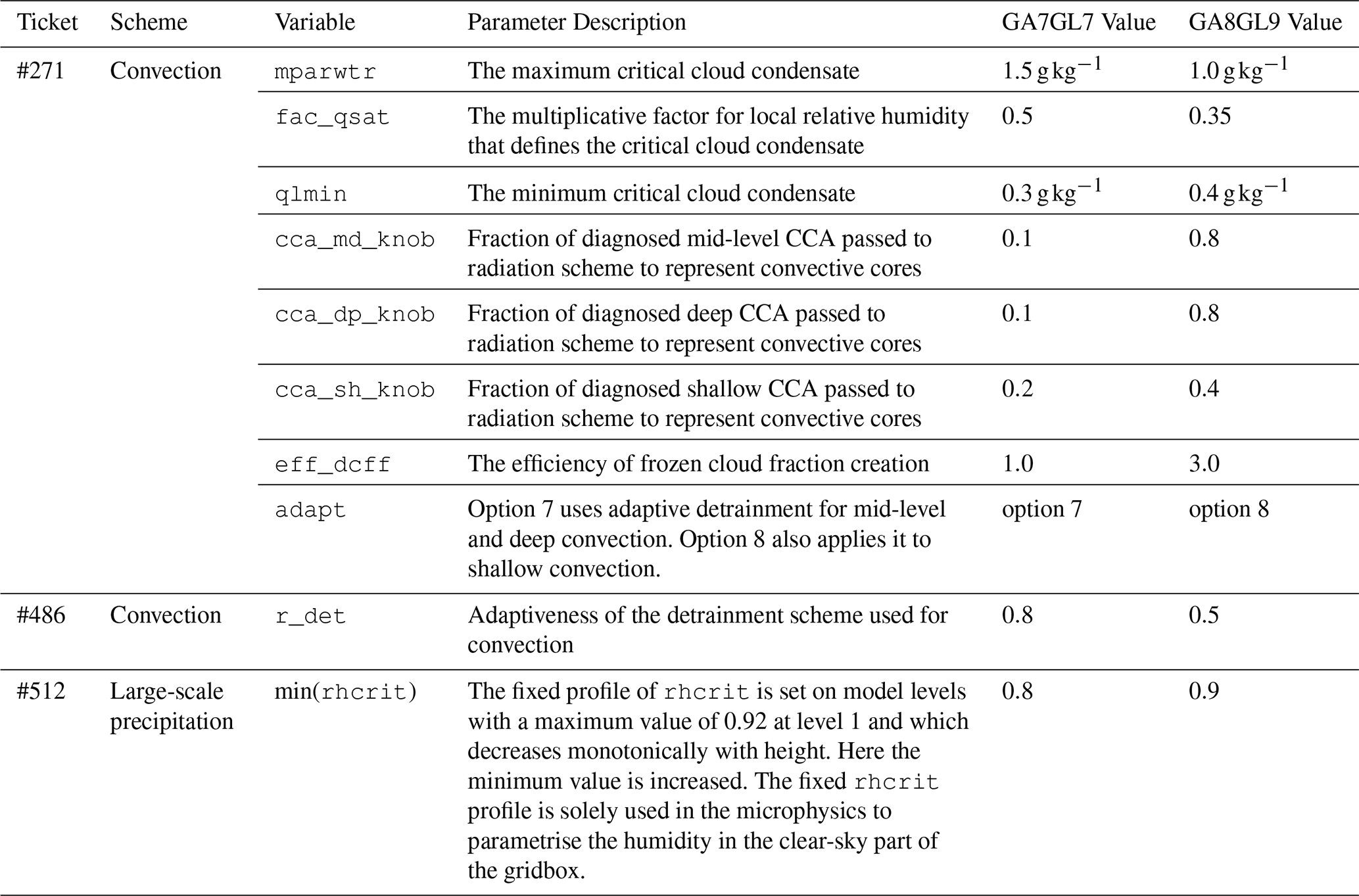
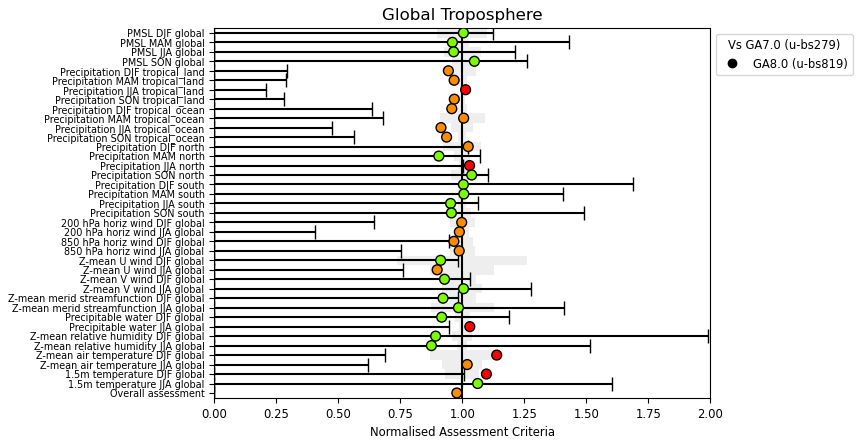
Figure 8 Normalised assessment plot (ratio of mean field RMSEs) for a number of atmospheric fields from a GA8GL9 atmosphere/land-only climate simulation at N216 horizontal resolution compared to an equivalent simulation using GA7GL7. Statistics shown are for seasons December-February (DJF), March–May (MAM), June–August (JJA) and September–November (SON) and for regions global, tropical land (land points between 30° N and 30° S), tropical ocean (sea points between 30° N and 30° S), north (30–90° N) and south (30–90° S). The observation datasets used are HadSLP2 pressure at mean sea level (Allan and Ansell, 2006), GPCP precipitation (Adler et al., 2003), SSMI precipitable water (Wentz and Spencer, 1998) and CRUTEM3 1.5 m temperature (Brohan et al., 2006), whilst the remaining climatologies are from ERA-interim reanalyses (Berrisford et al., 2009). The whisker bars are observational uncertainty, which is calculated by comparing these with alternative datasets; these are ERA-40 pressure at mean sea level and precipitable water (Uppala et al., 2005), CMAP precipitation (Xie and Arkin, 1997), Legates and Willmott (1990) 1.5 m temperature and MERRA reanalyses for everything else (Bosilovich, 2008). Green circles denote fields for which the RMSE lies within observational uncertainty, whilst light orange or red circles denote fields that do not, and for which the RMSE is improved or degraded respectively.

Table 10 Global- and annual-mean fluxes from 27 year N216 GA7GL7 and GA8GL9 AMIP simulations and observed estimates. The observed estimates of radiative fluxes are from CERES-EBAF edition 4.0 (Loeb et al., 2018) and the precipitation from GPCP version 3.2 (Huffman et al., 2023).

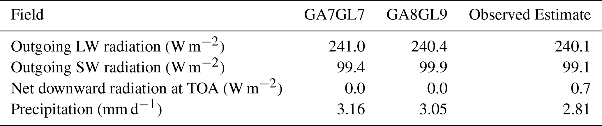
The day 5 tropical temperature biases in GA8GL9 and an untuned version of GA8GL9 are shown in Fig. 7. In the untuned version of GA8GL9 there is a large cold bias of up to 0.7 K between 600 and 700 hPa, and a warm bias of up 1.0 K centred around the tropical tropopause between 150 and 50 hPa. The cold bias was traced back in part to the introduction of the prognostic-based entrainment (Sect. 3.5.3). When there has been relatively little recent convective activity, the prognostic-based entrainment will use a relatively high entrainment rate, which will reduce parcel buoyancy, and usually results in more detrainment of convective condensate and associated cloud in the lower troposphere. This additional condensate and cloud then cools the environment through two mechanisms. Firstly, there is additional LW cooling from the top of cloud. Secondly the large-scale precipitation scheme (Sect. 2.4) relatively rapidly converts this detrained condensate from cloud into precipitation, which then evaporates and cools the environment. Decreasing the parameters that control the amount of convective parcel condensate at lower and mid-levels in the tropics (mparwtr and fac_qsat), reduces the amount of detrained cloud, and hence reduces the radiative and evaporative cooling. Reducing these two parameters in isolation also reduces the amount of low cloud in the tropics. The scalings applied to the CCA which is passed to radiation (cca_md_knob, cca_dp_knob and cca_sh_knob) are increased to compensate for the reduced low cloud and to compensate for the reduced CCAs seen with the new mass flux based CCA calculation (Sect. 3.5.6). The adaptive detrainment method was changed for shallow convection to make this tuning process easier. The increased warm bias around the tropical tropopause was again traced back to the prognostic-based entrainment. There is less cloud around the tropical tropopause because the prognostic-based entrainment results in deep convection detraining less condensate at higher levels; this results in less LW cooling from cloud top in the tropical tropopause region and hence an increased warm bias. To compensate for this, the parameters that control the amount of convective parcel condensate at higher levels (qlmin) and that control the amount of frozen cloud fraction created by detrained convective condensate (eff_dcff) are both increased. This increases the high cloud (both condensate and cloud fraction) in the tropics (and to a less degree elsewhere) which increases LW cooling from cloud top around the tropopause and reduces the warm bias at around 100 hPa. In isolation, however, this result in an undesirable warming in the upper tropical troposphere below the tropopause. The parameter r_det controls the adaptiveness of the adaptive detrainment scheme with larger values implying a wider range of buoyancies within each single plume (Derbyshire et al., 2011). As discussed in Willett and Whitall (2017), reducing r_det with the prognostic-based entrainment is justifiable, and arguably desirable, because the wider range of entrainment rates results in a wider range of buoyancies being represented amongst the convective plumes (i.e. at different times and locations), and it is no longer necessary to force such a wide range of buoyancies within each single plume with a large value of r_det. Reducing r_det cools the upper troposphere, which offsets the warming from the increased high-level cloud, and warms the lower and mid troposphere, which helps to further reduce the cold bias. The rhcrit profile, which is used to parametrise the humidity of the clear-sky and ice cloud only parts of the gridbox, is also modified because it reduces the cold bias between 600 and 700 hPa. As can be seen in a Fig. 7, the standard tuned version of GA8GL9 has substantially lower tropical temperature biases than the untuned version.

The global mean TOA radiative fluxes and global mean precipitation from the untuned and standard versions of GA8GL9 are compared to the observed estimates in Table 8. The untuned version of GA8GL9 has TOA radiative fluxes that are acceptably close to the observed estimates, and the constraint on the TOA radiative fluxes on its own would not have motivated a significant tuning exercise. After tuning the TOA radiative fluxes are, by design, acceptably close to observed estimates. The outgoing LW radiation is reduced, and the outgoing SW radiation is increased relative to the untuned version; this reflects a strengthening of both SW and LW TOA cloud forcing.

The tuned parameters and their GA7GL7 and GA8GL9 values are listed in Table 9. It should be noted that almost all scientific parameters in the model use the same values at all resolutions. The exceptions are several parameters that control the dust emission from the surface and the non-orographic gravity wave drag that use slightly different values at N96 than at all other resolutions. These parameters are routinely retuned as part of the GA/GL development process, but in GA8GL9, however, no additional tuning was found to be necessary and the values from Table 6 of Walters et al. (2019) are used.

4 Evaluation

GA7GL7 spawned a climate branch, GA7.1GL7.1, and the NWP branch, GA7.2GL8.1. Because of this, the detailed climate evaluation of GA8GL9 was made against GA7.1GL7.1 and the detailed NWP assessment was made against GA7.2GL8.1. A detailed assessment of GA8GL9 against these branch controls with a focus on coupled simulations is given in Xavier et al. (2024). However, a reduced assessment was made against GA7GL7 and this is presented here.

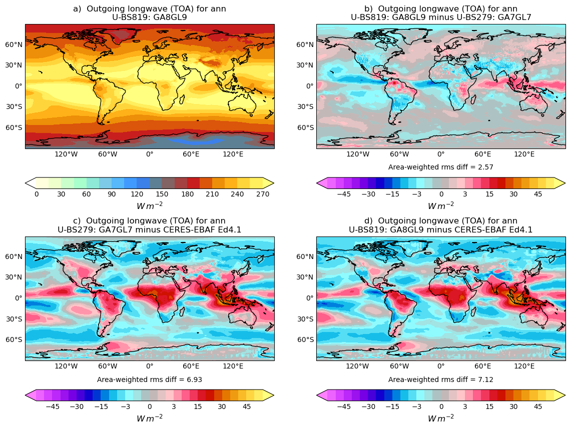
Figure 9 Annual mean top-of-atmosphere outgoing LW radiation (W m⁻²) in the 27 year N216 atmosphere/land only climate simulations compared to Clouds and Earth's Radiant Energy System (CERES) Energy Balanced and Filled (EBAF)dataset version 4.1 (NASA/LARC/SD/ASDC, 2019) showing (a) GA8GL9, (b) the difference between GA8GL9 and GA7GL7, (c) bias in GA7GL7 relative to CERES-EBAF and (d) bias in GA8GL9 relative to CERES-EBAF.

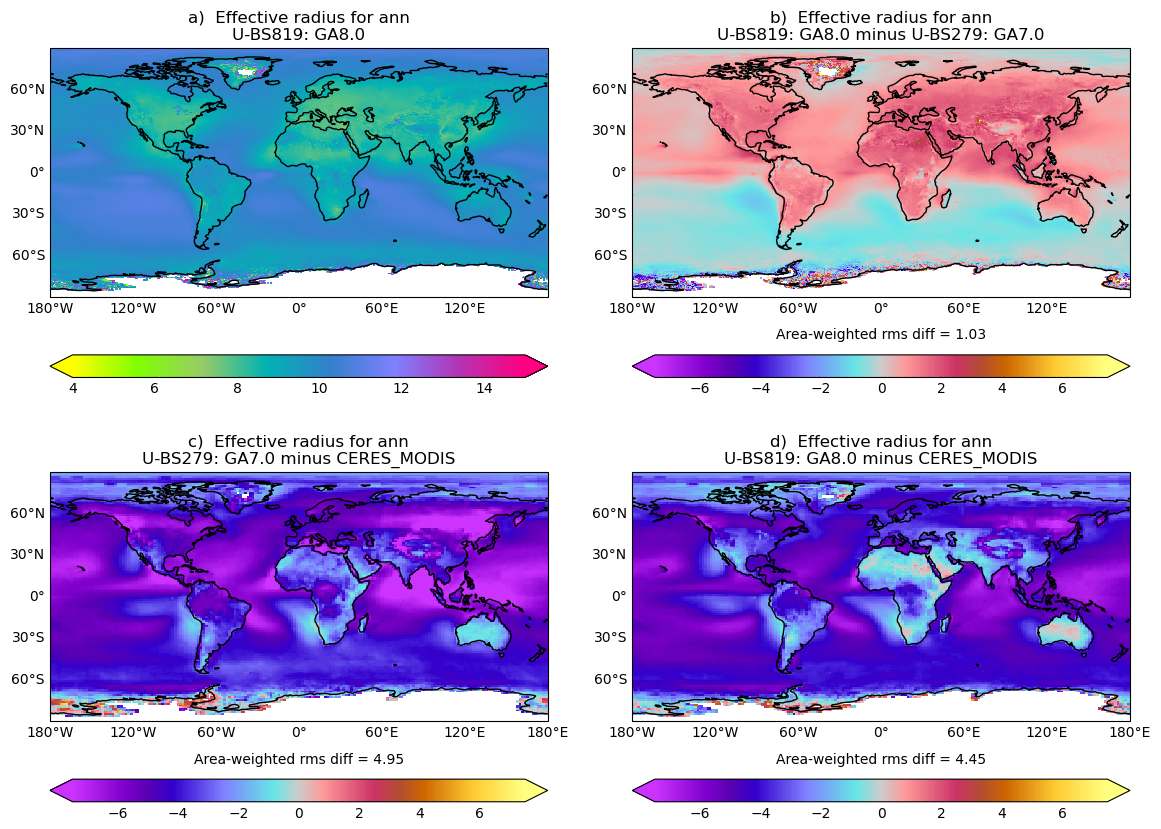
Figure 10 Annual mean cloud droplet effective radius (µm) in the 27 year N216 atmosphere/land only climate simulations compared to Clouds and Earth's Radiant Energy System (CERES) Moderate Resolution Imaging Spectrometer (MODIS) Edition 2.6. Layout is the same as in Fig. 9.

4.1 Climate Assessment

The climate performance of GA8GL9 was compared to GA7GL7 using 27 year long atmosphere/land only climate simulations at both N96L85 and N216L85 resolutions. We focus here on the N216L85 simulations, but the results are consistent across both resolutions unless explicitly discussed in the text.

Figure 8 shows a top-level summary of the impact of GA8GL9 relative to GA7GL7 on the model's climatology as measured by the ratio of spatial RMSE of various meaned fields with respect to a range of observational estimates and reanalyses. The majority of the fields presented here are either improved, little changed or within observational uncertainty. The zonal-mean temperature bias relative to ERA-interim in DJF is slightly degraded but this primarily due to a cooling in the mid-, tropical-troposphere. This is not considered to be an substantial issue because NWP tests of GA8GL9 show little bias with respect to radiosondes even at longer forecast times.

Global and annual mean fluxes from the model simulations as well as observational estimates are given in Table 10. The TOA global and annual mean Top of Atmosphere (TOA) radiative fluxes are similar in GA7GL7 and GA8GL9 and both are close to observed values. This is largely because both model configurations have been tuned to give values close to observed estimates. As was noted in Walters et al. (2019), GA7GL7 had an overactive hydrological cycle and this bias as measured by the global mean precipitation has been reduced in GA8GL9.

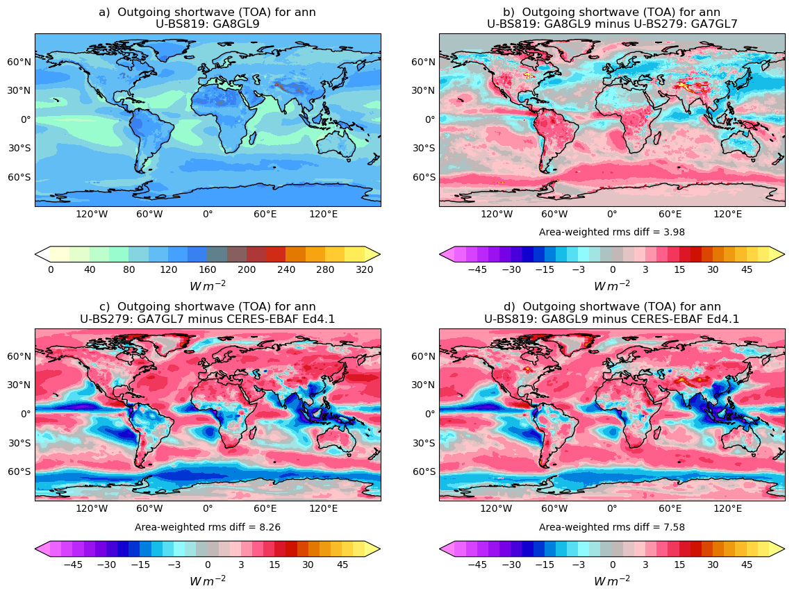
Figure 11 Annual mean top-of-atmosphere outgoing SW radiation (W m⁻²) in the 27 year N216 atmosphere/land only climate simulations compared to Clouds and Earth's Radiant Energy System (CERES) Energy Balanced and Filled (EBAF) dataset version 4.1 (NASA/LARC/SD/ASDC, 2019). Layout is the same as in Fig. 9.

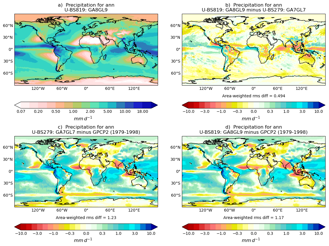
Figure 12 Annual mean precipitation (mm d⁻¹) in the 27 year N216 atmosphere/land only climate simulations compared to GPCP (Adler et al., 2003). Layout is the same as in Fig. 9.

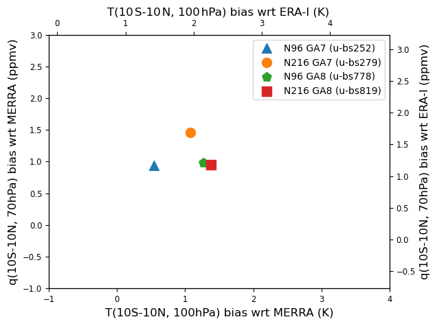
Figure 13 Tropical tropopause layer temperature biases and lower stratospheric humidity biases from 27 year N96 and N216 atmosphere/land-only climate simulations of GA7L7 and GA8L9 with respect to MERRA and ERA-Interim reanalyses (following Hardiman et al., 2015).

GA8GL9 and GA7GL7 both show similar spatial error structures in outgoing LW radiation (OLR) when compared to CERES-EBAF (Fig. 9). The OLR in the tropical Indian Ocean, maritime continent and western Pacific Ocean increases in GA8GL9 which is mostly detrimental; in the tropical Atlantic and east Pacific Ocean the OLR reduces which is mostly beneficial. Overall the errors relative to CERES-EBAF in GA8GL9 are similar to those in GA7GL7 in the annual mean (shown here) and in the individual seasons.

The cloud condensate effective radius is increased over land and much of the northern hemisphere oceans, and reduced over southern hemisphere oceans (Fig. 10) largely as a result of the Liu spectral dispersion (Sect. 3.2.1) and TKE diagnostic improvements (Sect. 3.4.4). A negative bias still remains compared to MODIS (although noting that comparisons with other estimates do not show such a large negative bias and that MODIS is believed have a positive bias, e.g. Fu et al., 2022), but the error is reduced relative to GA7GL7 and the bias is less spatially variable. The annual mean outgoing SW errors are reduced in GA8GL9 relative to GA7GL7 (Fig. 11). Much of the reduction in outgoing SW in the northern hemisphere and increase in the southern hemisphere is due to the changes in the effective radius, but the beneficial large increase in outgoing SW at around 60° S are due to the improved representation of mixed phase processes (Sect. 3.3.1). The beneficial increases in outgoing SW over tropical land are largely due to a combination of the convection changes and the tuning.

The reduced hydrological strength can be seen in Fig. 12 with a clear reduction in precipitation in the extratropics. The precipitation is beneficially reduced over central Africa and the equatorial Indian Ocean whilst the drying over Australia acts to increase the pre-existing dry bias. Overall, the annual mean precipitation has only slightly improved the agreement with GPCP precipitation.

As noted in Walters et al. (2019), the tropical tropopause layer (TTL) temperature and humidity biases in GA7GL7 degrade between N96 and N216 resolutions. However, in GA8GL9 the biases are essentially independent of resolution (Fig. 13) which is largely due to the improved convection-dynamics coupling (Sect. 3.5.1).

Overall, the mean climate in GA8GL9 is improved relative to GA7GL7 with small improvements over the majority of fields, and notable improvements in the SW radiative fluxes as described above. There are modest improvements in the diurnal cycle (Sect. 3.5.1) and the effects of convective intermittency are reduced (Sect. 3.5.3). Other modes of variability that were assessed in these climate simulations, e.g. the MJO, African easterly waves and QBO, were largely unchanged.

4.2 NWP Assessment

The NWP performance of GA8GL9 was compared to GA7GL7 using 3-month long atmosphere/land only DA trials at a resolution of N640L70 covering September to November 2019. The same DA setup was used for both model configurations. The DA setup uses 4-dimensional variational (4DVar) DA (Rawlins et al., 2007) and a variational bias correction (Cameron and Bell, 2018) for the majority of the observations. Each model configuration will have its own analyses, from which forecasts will be initialised and which their forecasts are verified against, because of the coupling to the DA system. Figure 14 shows a top-level summary of the impact of GA8GL9 relative to GA7GL7 for a range of fields at different forecast time as measured by the fractional change in RMSE and verified against observations and own analysis. When averaged over all the fields and forecast times shown, the RMSE is reduced by 1.3 % and 1.5 % against observations and own analyses respectively. Some fields have higher RMSE in GA8GL9, for example the RMSE in tropical winds at 250 hPa when verified against their own analyses. It should be noted that this is largely attributable to the increased spatial variability in GA8GL9 in both forecasts and own analyses, which is in itself due to greater structure in the diabatic forcing.

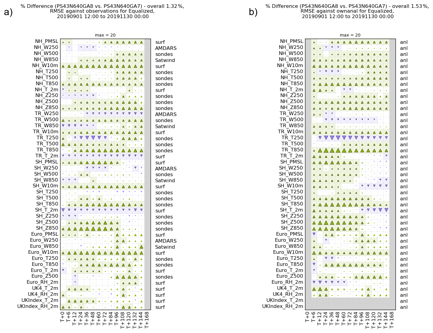
Figure 14 Global evaluation suite scorecards for GA8GL9 vs. GA7GL7 for a three month N640 DA non-hybrid trial for September, October and November 2019 with respect to (a) observations and (b) own analysis. Shaded boxes are statistically significant. Green upward pointing triangles indicate the RMSEs in GA8GL9 are reduced relative to GA7GL7, and downward pointing purple triangles indicate where the RMSEs are increased. The area of the triangles is proportional to the change in RMSE with a change of 5 % filling the box.

A particular aim of GA8GL9 development was to improve the tropical temperature structure relative to GA7GL7. Figures 15 and 16 show the temperature biases and RMSE at day 1 and day 5 respectively. The warm bias at 850 hPa and cold bias at 600 hPa seen in GA7GL7 are both reduced in GA8GL9. GA8GL9 is slightly cooler than GA7GL7 in the upper tropical troposphere, but this counteracts the warm bias seen in GA7GL7 relative to sondes at longer forecast times. Even at day 5, the tropics mean biases below the tropopause in GA8GL9 are all less than 0.3 K.

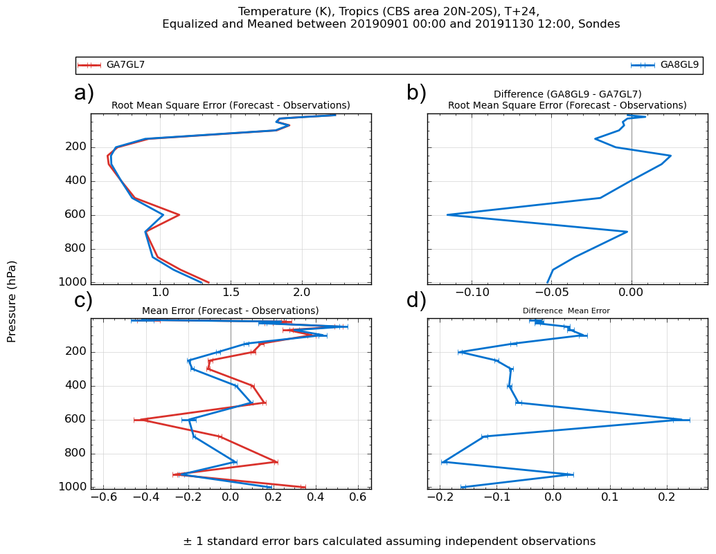
Figure 15 Verification with respect to sondes of tropical T + 24 temperatures forecasts from GA7 and GA8 showing (a) RMSE, (b) difference in RMSE, (c) mean error, and (d) difference in mean error for the three month N640 DA non-hybrid trial for SON 2019.

Figure 16 As Fig. 15 but for T + 120.

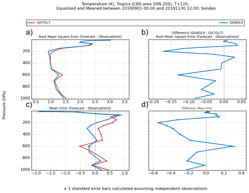
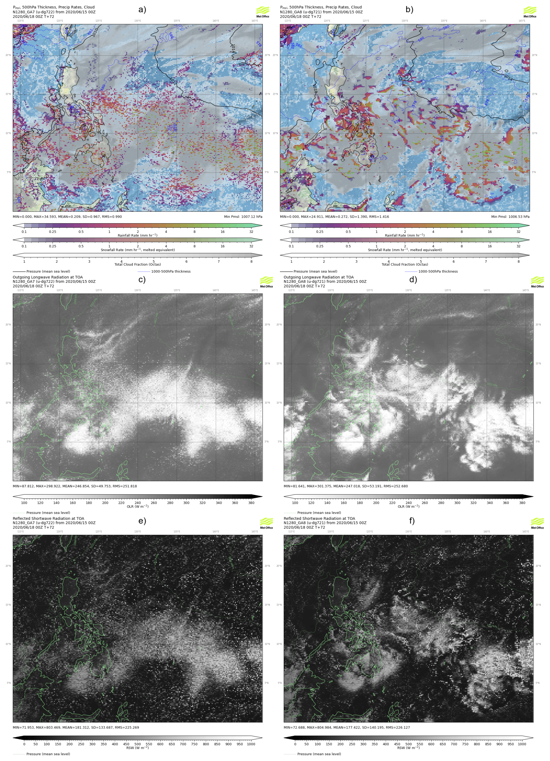
Figure 17 T + 72 forecasts of instantaneous precipitation in colour and total cloud in grey (top row), outgoing LW radiation (middle row) and outgoing SW radiation (bottom row) from N1280 simulations using GA7GL7 (a, c, e) and GA8GL9 (b, d, f) for a region of the west Pacific ocean. Background map generated using Cartopy (Met Office, 2010–2015). Credit: Made with Natural Earth.

Figure 17 shows an example of instantaneous precipitation, cloud fraction, outgoing LW radiation and outgoing SW radiation from an N1280 (nominally 10 km) case study. It can be clearly seen that GA8GL9 has more fine scale structure but less grid scale noise in the precipitation and radiative fluxes. This example is typical of the differences seen at higher model resolutions in regimes where convection is very active; this effect is present at lower resolutions but can be more subtle. This improvement is primarily due to the prognostic-based entrainment rate (Sect. 3.5.3). The increase in structure in the diabatic forcing results in an increase in the spatial power of the forecast winds at scales below approximately 1000 km as can be seen in the zonal power spectra in Fig. 18. Similar increases are also seen in the spatial spectra of other forecast fields such as temperature, relative humidity, cloud condensate, outgoing LW and outgoing SW at all forecasts times and also at analysis time.

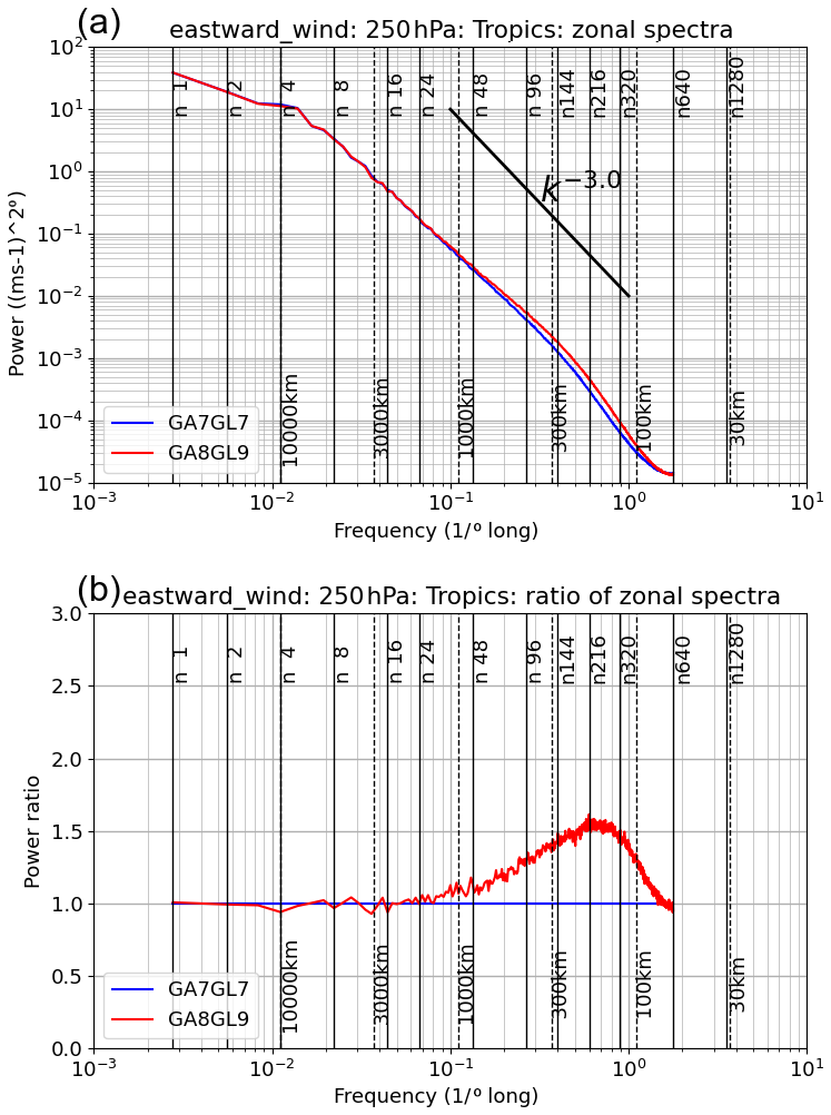
Figure 18 Zonal power spectra of tropical 250 hPa winds from GA8GL9 and GA7GL7 from 00:00 and 12:00 Z forecasts during November from the N640 DA trial showing (a) the absolute spectra and (b) the ratio relative to the GA7GL7 spectra.

The overall NWP performance of GA8GL9 substantially improves upon the performance of GA7GL7. The verification scores are consistently improved despite increases in spatial varibility, and there are visible improvements in fine scale spatial structure. The level of improvement was such that GA8GL9 in its coupled configuration, GC4, replaced the NWP specific branch GA7.2GL8.1 as the operational global NWP model at the Met Office.

5 Conclusions

GA8GL9 builds upon GA7GL7 and not only consolidates the changes made for the branch configurations GA7.1GL7.1 and GA7.2GL8.1, but also includes changes to most areas of the science. These include the prognostic-based entrainment, which improves the spatial structure of convection, time-smoothed convective increments and an addition termination condition for convection which both reduce tropical tropopause biases, a new riming parametrisation which improves SW biases in the Southern Ocean, and a package of surface changes which remove the need for an aggregate tile in NWP applications. The introduction of the multigrid solver greatly reduces the amount of numerical noise at the poles, and the improvement to computational stability of the CMT prevents the CMT from generating numerical noise in the wind increments. The addition of a lower limit to the CAPE timescale greatly reduces the frequency of spurious convectively coupled waves. Increasing the non-linear solver term for unstable BLs greatly reduces the likelihood of a relatively common failure mechanism. More realistic treatments of melting snow and freezing rain in the convection scheme and changes to BL scheme should reduce the sensitivity to vertical resolution and therefore facilitate any future increases in vertical resolution. In summary, GA8GL9 improves upon its immediate predecessor GA7GL7 in terms of scientific performance and numerical properties, and as such is not only suitable for operational implementation but also provides a solid basis for future GA/GL configurations.