Modelling framework for asynchronous land-atmosphere coupling using NASA GISS ModelE (NASA-GISS E2.1) and LPJ-LMfire (v1.4.0): design, application and evaluation for the 2.5 ka period

While paleoclimate simulations have been a priority for Earth system modelers over the past three decades, little attention has been paid to the period between the mid-Holocene (6 ka) and the Last Millennium, although this is an important period for the emergence of complex societies. Here, we consider the climate of 2500 BP (before present or 550 BCE), a period when compared to late preindustrial time, greenhouse gas concentrations were slightly lower, and orbital forcing led to a stronger seasonal cycle in high latitude insolation. To capture the influence of land cover on climate, we asynchronously coupled the NASA GISS ModelE Earth system model with the LPJ-LMfire dynamic global vegetation model. We simulated global climate and assessed our results in the context of independent paleoclimate reconstructions. We also explored a set of combinations of model performance parameters (bias and variability) and demonstrated their importance for the asynchronous coupling framework. The asynchronously coupled model system shows strong vegetation-albedo feedback on climate and is comparatively more sensitive to the bias correction than the internal model variability and green Sahara conditions. In the absence of a bias correction, while driving LPJ-LMfire in the coupling process, ModelE drifts towards colder conditions in the high latitudes of the Northern Hemisphere in response to land cover simulated by LPJ-LMfire. A regional precipitation response is also prominent in the various combinations of the coupled model system, with a substantial intensification of the Summer Indian Monsoon and a drying pattern over Europe. Evaluation of the simulated climate against reconstructions of temperature from multiple proxies and the isotopic composition of precipitation (δ¹⁸O_p) from speleothems demonstrated the skill of ModelE in simulating past climate. A regional analysis of the simulated vegetation-climate response further confirmed the validity of this approach. The NASA GISS ModelE was found to be particularly sensitive to the representation of shrubs and this land cover type requires particular attention as a potentially important driver of climate in regions where shrubs are abundant. Our results further demonstrate the importance of bias correction in coupled paleoclimate simulations. This study presents a generalized framework for incorporating biogeophysical responses into climate models without dynamic vegetation, for simulating past climates, in line with the recommendations of the Paleoclimate Modelling Intercomparison Project (PMIP).

1 Introduction

Earth system models (ESMs) are widely applied in paleoclimate experiments as an “out of sample” exercise to evaluate the overall quality of the model, and to better understand climate system responses to external forcings. In many paleoclimate modeling studies, it has been demonstrated that the inclusion of biogeophysical and biogeochemical feedbacks between land and atmosphere are essential to simulate the magnitude and spatial pattern of climate change that is consistent with independent reconstructions (Betts, 2000; Claussen, 1997; Cox et al., 2000; Doherty et al., 2000; Strandberg et al., 2014a). The importance of land-atmosphere feedbacks for past climate has been shown to be particularly high in the context of the mid-Holocene and last glacial inception periods (Braconnot et al., 2012; Collins et al., 2017; Harrison et al., 2015; Jahn et al., 2005; Kubatzki and Claussen, 1998; Sha et al., 2019; Shanahan et al., 2015; Tierney et al., 2017). For example, for the African Humid Period of the mid-Holocene, numerous studies have demonstrated that greenhouse gases (CO₂, N₂O, CH₄) and orbital forcing are alone insufficient for models to simulate climate that is consistent with independent paleoclimate reconstructions. The inclusion of land-atmosphere feedbacks via interactive dynamic vegetation modeling or prescribed vegetation distributions helps to reduce model-proxy discrepancies (Chandan and Peltier, 2020; Charney, 1975; Dallmeyer et al., 2021; Pausata et al., 2016; Rachmayani et al., 2015; Singh et al., 2023; Thompson et al., 2021; Tiwari et al., 2023; Velasquez et al., 2021). For this reason, more recent protocols (PMIP4; Otto-Bliesner et al., 2017) for simulations of the mid-Holocene specify that the land cover boundary condition should include shrub vegetation in northern Africa with greater extent than the present (the so-called “Green Sahara”), as well as an expansion of trees and shrubs at high northern latitudes.

Instead of prescribing land cover boundary conditions in an earth system model, it may be desirable to employ a coupled model where that allows interaction between climate and vegetation. While several modern earth system models include a dynamic representation of land cover, in climate models (regional and global) that lack a coupled dynamic vegetation component a well-established technique to capture land-atmosphere feedbacks is to use asynchronous coupling. In this type of coupling, climate model output is used to drive an offline vegetation model that then returns a land cover boundary condition to the climate model.

To quantify the feedback between land and atmosphere and improve the fidelity of the paleoclimate simulation, asynchronous coupling typically involves running a climate model simulation for a period of a few decades, after which the mean climate state is passed to a vegetation model that in-turn produces a land cover boundary condition for the climate model. This process is repeated until climate reaches equilibrium, defined as insignificant changes in key outputs, e.g., 2 m temperature, from one cycle to the next.

Texier et al. (1997) used an iterative asynchronous coupling between the LMD Atmospheric General Circulation Model (AGCM) and the BIOME1 vegetation model to produce an improved climate for the mid-Holocene (6 ka) period and found that inclusion of land-atmosphere feedbacks led to simulations of temperatures at high latitudes and precipitation over West Africa that were more consistent with independent paleoclimate reconstructions compared to atmosphere-only simulations. de Noblet et al. (1996) used a similar coupling to highlight the role of biogeophysical feedback in glacial initiation around 115 ka ago. Asynchronous coupling has also been used with regional climate models (RCMs). Kjellström et al. (2009) and Velasquez et al. (2021) both used asynchronous coupling between an RCM and land cover model to simulate the climate of Europe at the Last Glacial Maximum. Both studies demonstrated the importance of land cover in improving agreement with reconstructions and paleoenvironmental proxies.

This study has two objectives. First, we present a generalized design for asynchronously coupling the NASA GISS ModelE2.1 climate model (Kelley et al., 2020) with the LPJ-LMfire DGVM (Pfeiffer et al., 2013) to simulate climate and include biogeophysical land-atmosphere feedbacks. Second, we demonstrate the utility of this asynchronous coupling framework for a paleoclimatic period that has not been the traditional focus of paleoclimate modeling (2.5 ka) and evaluate the model results against independent paleoclimate reconstructions for that period.

2.5 ka represents a time that is nearest to the present day among the different periods selected under the coordinated effort of the Paleoclimate Model Intercomparison Project (PMIP4). It is interesting because it represents an important period for the emergence of complex societies across Eurasia (Iron Age, Classical Antiquity, early Imperial China) and elsewhere. During this era, favorable climate conditions around the Mediterranean might have influenced the emergence of the golden age of Greece, the Roman classical period, and other empires of Southern Europe, North Africa, and southwest Asia (Lamb, 1982; Reale and Dirmeyer, 2000). On the other hand, adverse climate conditions due to volcanic eruptions and a series of arid phases during this period may have had a negative impact on Egyptian civilization around the Nile and Mesopotamian civilization around the Euphrates and Tigris rivers. 2.5 ka is thus a key period for the study of human-environment interactions and the history of climate and society, where we may assess societal vulnerability to climate variability on different scales (Ludlow and Manning, 2021; Manning et al., 2017; Mikhail, 2015; Petit-Maire et al., 1997; Singh et al., 2023).

Section 2 describes the models used in this study (Sect. 2.1), the initial control run for 2.5 ka, and a stepwise description of the asynchronous coupling framework, including variable exchange and processing (Sect. 2.2 and 2.3). Section 3 presents the experimental design for implementing the asynchronous coupled system and evaluates the PFT mapping schemes. In Sect. 4, we evaluate the simulated 2.5 ka climate using the ModelE–LPJ asynchronous coupling framework against multi-proxy temperature reconstructions (Kaufman et al., 2020) and additionally utilized the model's capabilities to simulate the isotopic composition of water in precipitation (δ¹⁸O_p) to compare with the Speleothem Isotope Synthesis and Analysis (SISAL) version 2 database (Comas-Bru et al., 2020). Section 5 provides the analysis and comparison of model-simulated climate under various experimental configurations.

2 Models and asynchronous coupling framework

2.1 Models

2.1.1 NASA GISS ModelE2.1

NASA GISS ModelE2.1 (Kelley et al., 2020) is the climate model of the NASA Goddard Institute for Space Studies (GISS) currently used in Climate Model Intercomparison Project (CMIP) phase 6 (Eyring et al., 2016). We used the NINT (Non-Interactive; physics version 1 in CMIP6) GISS ModelE2.1 version where aerosols and ozone are precomputed from the prognostic, but much more computationally demanding, chemistry and aerosols version of the model OMA (One Moment Aerosols; physics version 3 in CMIP6; Bauer et al., 2020). In our simulations, the GISS ModelE2.1 atmosphere has a horizontal resolution of 2° × 2.5° (latitude/longitude) with 40 vertical layers, and the top of the atmosphere at 0.1 hPa. The ModelE2.1 atmosphere has a smooth transition from sigma layers to constant pressure layers centered at 100 hPa. The atmosphere is coupled to the GISS Ocean v1 model, which runs at a resolution of 1° × 1.25° (latitude/longitude) with 40 depth layers to the ocean bottom. While the biogeophysical properties of land cover are simulated with the Ent Terrestrial Biosphere Model (Ent TBM; Kiang 2012; Kim et al., 2015), as part of ModelE2.1 (Ito et al., 2020), Ent relies on a prescribed vegetation map and as such does not simulate changes in land cover over time. To capture the influence of climate change on land cover and biogeophysical feedbacks between land and atmosphere, asynchronous coupling with LPJ-LMfire (or any other DGVM) is currently required.

2.1.2 LPJ-LMfire

We used the LPJ-LMfire DGVM (v1.4.0) to simulate the land cover boundary conditions in our experiments. LPJ-LMfire (Kaplan et al., 2022; Pfeiffer et al., 2013) is an evolution of LPJ (Sitch et al., 2003) and is a process-based, large-scale representation of plant growth and decay, vegetation demographics and ecological disturbance, and water and carbon exchanges between the land and the atmosphere. LPJ-LMfire has been successfully validated for simulating present-day biogeography and fire regime characteristics, and its outputs have been compared against contemporary observations (Pfeiffer et al., 2013; Sitch et al., 2003; Thonicke et al., 2010). For this study, we simulated land cover boundary conditions at a horizontal resolution of 0.5° × 0.5°. LPJ-LMfire is driven by monthly climate fields (temperature, precipitation, cloud cover, wind, and lightning), static maps of topography and soil texture, and an annual global value of atmospheric CO₂ concentration. LPJ-LMfire simulates land cover in the form of fractional coverages of nine plant functional types (PFTs), including tropical, temperate, and boreal trees, and tropical and extratropical herbaceous vegetation (Table 1). CO₂, soil texture and topography data used to drive LPJ-LMfire are described in Pfeiffer et al. (2013, Table 3). For 2.5 ka simulations, we set atmospheric CO₂ concentrations to 271.4 ppm (Kaplan et al., 2012). The sum of PFT fractional cover per grid box does not need to equal unity; when it is less than one the remainder is considered bare ground.

Table 1 Summary of climate and land cover variables exchanged between NASA GISS ModelE and LPJ-LMfire model for asynchronous coupling process. Column 1 and 2 shows the output and input climate variables from GISS ModelE to LPJ-LMfire models, whereas the columns 3 and 4 lists the output and input plant functional types (PFTs) from LPJ-LMfire to GISS ModelE.

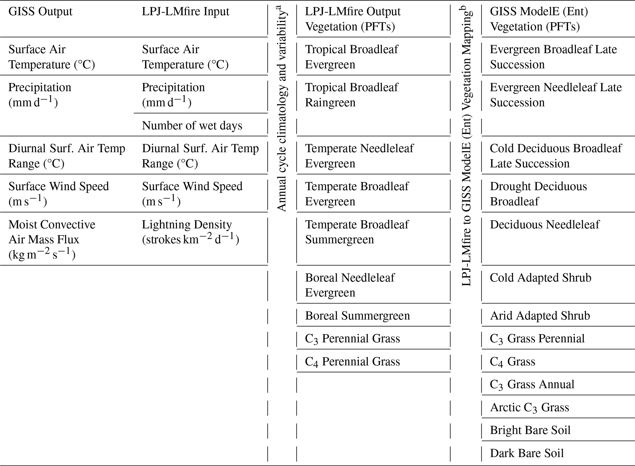
^a Variability is one standard deviation over the period of interest (100 Years). ^b The mapping was applied to vegetation cover type, Leaf area index, and vegetation height.

2.2 2.5 ka Simulation setup (Initial control run using ModelE)

We started the 2.5 ka and preindustrial (PI) control experiments following the PMIP4 and CMIP6 protocols (Eyring et al., 2016; Kageyama et al., 2018). The PI simulation uses preindustrial (year 1850) GHG concentrations and a modern continental configuration and serves as the reference experiment for designing the boundary conditions for past time slices studied in PMIP4. GHG and orbital forcings for the preindustrial (PI) control experiment correspond to levels observed in 1850 CE (CO₂: 284 ppm, N₂O: 273 ppb, CH₄: 808 ppb). For the 2.5 ka control experiment, orbital parameters (Berger et al., 2006) were specified for 2500 years BP (before present ∼ 550 BCE), and greenhouse gas CO₂, N₂O, and CH₄ were set to ∼ 279, ∼ 266, and 610 ppb, respectively (Köhler et al., 2017; Loulergue et al., 2008; Otto-Bliesner et al., 2017; Schneider et al., 2013; Siegenthaler et al., 2005). We considered only natural emissions as sources of aerosols in the atmosphere, zeroing-out any anthropogenic contribution to aerosol and aerosol precursors. For biomass burning, in the absence of any better estimate, we assumed that the emissions provided by CEDS (Hoesly et al., 2018) for the year 1750 are all natural. Land cover consists of the fractional coverages of 13 plant functional types (PFTs) and includes vegetation height and leaf area index (LAI). For the PI and initial (0th order) simulations, land cover type and monthly-varying LAI were derived from satellite (MODIS) data (Gao et al., 2008; Kattge et al., 2011; Myneni et al., 2002; Tian et al., 2002a, b; Yang et al., 2006) and vegetation height from Simard et al. (2011). We also used the mid-Holocene (6 k) vegetation under the PMIP4 protocol, which is linearly interpolated to 2.5 ka period and details of vegetation cover changes (Singh et al., 2023; Fig. S2 in the Supplement) and associated impacts on the northern hemisphere climate due to the inclusion of scaled PMIP4 vegetation using the interactive chemistry version of NASA GISS ModelE2.1 (MATRIX) are discussed in Singh et al. (2023).

2.3 Asynchronous coupling framework

The asynchronous coupling between ModelE and LPJ-LMfire is summarized in Fig. 1. For each iteration, ModelE simulated climate is used by LPJ-LMfire which returns the PFT fractional cover, LAI, and vegetation height that are used as boundary conditions for the next ModelE simulation.

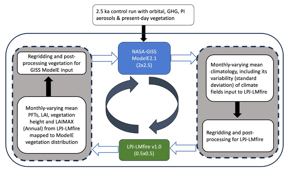
Figure 1 Flow diagram for the asynchronous coupling framework between GISS ModelE2.1 and LPJ-LMfire models. For the climate fields input to LPJ-LMfire refer to (Table 1, Column 1) and LPJ-LMfire PFTs (Table 1, Column 3).

2.3.1 GISS ModelE2.1 simulations

Climatological monthly mean climate (Table 1, Column 1) for a 100-year period was extracted from a well equilibrated ModelE simulation. To assess interannual variability with monthly resolution, we calculated the standard deviation of the decadal mean data for each month across the 100-year equilibrium period.

2.3.2 LPJ-LMfire simulations

All climate variables except diurnal temperature range, wet days, and lightning density were provided directly from the ModelE output. For derived climate variables, the additional processing steps are described below.

Diurnal temperature range was calculated as the difference of the monthly-mean daily maximum and minimum temperatures as simulated by ModelE. Wet days were calculated from modelled precipitation based on an empirical relationship between present-day monthly total precipitation and the number of wet days per month. To quantify this relationship, we performed a nonlinear regression between monthly total precipitation and the number of days with measurable precipitation using the CRU TS 4.0 gridded climate fields (Harris et al., 2020). Using those data, we developed a set of regression coefficients for every land gridcell that allowed us to estimate wet days for any paleoclimate period based only on monthly total precipitation. Lightning density was estimated based on modelled convective mass flux following Magi (2015). However, the feedback to climate due to fire-driven emissions are not included, as accounting for them would require active atmospheric chemistry and transport, which are not included in LPJ-LMfire.

Because LPJ-LMfire requires a timeseries of interannually varying climate forcing to run, we processed the climatological monthly mean climate produced by the ModelE for use with the vegetation model. In brief, ModelE climate was converted into anomalies by differencing the paleoclimate simulation with ModelE simulated climate for the late 20th century (1951–2000). The resulting climate anomalies were bilinearly interpolated to a 0.5° × 0.5° grid and added to a baseline climate based on observations over 1951–2000. The resulting climatology was expanded to a 1020-year-long time series by adding interannual variability in the form of detrended and randomized climate anomalies from the 20th Century Reanalysis (Compo et al., 2011). LPJ requires climate input data with interannual variability because fires and other disturbance events occur only in years with anomalous climate, for example, hot or dry years Sitch et al. (2003). Driving the model with climatological mean climate will result in disturbance frequencies that are lower than the expected mean that in some regions would lead to an overabundance of tree cover when we would expect herbaceous vegetation. For further details on this process, see (Hamilton et al., 2018). Because LPJ-LMfire is computationally inexpensive, we ran each simulation for 1020 years. While the composition and characteristics of aboveground vegetation comes into equilibrium with climate after a few centuries of simulation, a millennium-long simulation brings the terrestrial carbon pools into equilibrium as well. The land cover boundary conditions returned to the climate model represent the mean modeled vegetation cover over the final 250 years of the LPJ-LMfire simulation.

2.3.3 LPJ-LMfire to GISS ModelE vegetation mapping

LPJ-LMfire simulates land cover in the form of nine PFTs, while in GISS ModelE the vegetation component (Ent TBM) recognizes 13 PFTs. We mapped the LPJ-LMfire generated PFT cover, LAI, LAIMAX, and vegetation height to the GISS ModelE2.1 (Ent) PFTs in order to feed it to the ModelE (Table 1, Column 3 & 4). The main points for the LPJ-LMfire to GISS vegetation mapping are the following:

• Early and late-successional PFTs were approximated from the LPJ-LMfire output using the model simulated fire frequency and monthly burned area fraction. High fire frequency favors early-successional PFTs because the time between disturbances is shorter than that required for establishment. By definition, late-successional PFTs require extended periods of low disturbance to persist within the ecosystem. However, because successional state is indistinguishable in the satellite-driven reference vegetation for the historical period used as the boundary condition for ModelE, we combined early and late successional PFTs in our simulations.

• LPJ-LMfire does not have a specific PFT for shrubs (arid and cold), while Ent does. To estimate shrub cover in LPJ-LMfire, we used LPJ-LMfire simulated tree height for the tropical broadleaf raingreen, temperate broadleaf summergreen, and boreal summergreen PFTs and specified that trees with height lower than a globally-uniform predefined threshold were considered to be shrubs (Table S1 in the Supplement).

• Ent has an Arctic grass PFT while LPJ-LMfire does not. To estimate Arctic grass cover we used the C₃ grass PFT in LPJ-LMfire and specified it as Arctic grass in regions where the boreal summergreen PFT was also present. LPJ-LMfire also does not distinguish between annual and perennial grasses, and so to map these to Ent we assumed that these were present in equal fractions among the simulated C₃ grass in the LPJ-LMfire simulation.

• The non-vegetated fraction of a grid cell is assigned to the bare soil, and the distribution of bright and dark soil color heterogeneity is classified/redistributed based on the present-day structure of soils over a grid cell.

Of particular importance to our coupled model simulations was that the PFTs simulated by LPJ-LMfire do not explicitly include a shrub type. To approximately distinguish tree from shrub cover, we generated three LPJ-to-GISS mapping schemes that differed on how shrubs are specified. A set of possible changes in various PFT classifications are adopted based on the comparison with GISS vegetation distribution and the categorized mapping methodologies. These mappings, summarized in Table S1, differ in the height threshold of trees to be re-categorized as cold and arid shrubs, and the fraction of perennial grass re-categorized into perennial and arctic grasses. Also, the monthly leaf area index (LAI) and vegetation height is readjusted using the weighted mean for remapped LPJ-LMfire vegetation PFTs.

2.3.4 Step 4: Post-processing of vegetation files

LPJ-LMfire model generates output at a horizontal resolution of 0.5° × 0.5°. We resampled the output vegetation information to the 2.0° × 2.5° grid used by ModelE2.1. In a few cases, land cover extrapolated using a nearest-neighbor approach was to cover all the grid cells identified as land in the ModelE standard land-sea mask.

3 Experimental Design

Apart from evaluating the framework for the PI control period, we designed a set of experiments to evaluate various aspects of the simulated climate, including model bias, and variability in both the climate and vegetation models. For example, one known limitation in the current version of ModelE is a wintertime cold bias over the Arctic in simulations covering the historical period (Kelley et al., 2020).

Table 2 shows the combinations of the model metrics selected to explore the utility of the asynchronous coupling framework and their impact on simulated climate. Run names are designated using Time (1850, 2.5 k), Vegetation source (PI, GS), Bias Correction (BC) and Interannual Variability (LPJ, GISS) separated by “_”. For example, “1850_PI_ctrl” and “2.5k_PI_ctrl” denote the 1000-year-long PI and 2.5 k runs with GISS PI vegetation. GS stands for Green Sahara and PI = Pre-Industrial. An “x” denotes the absence of a particular criterion (default state). Run “1850_PI_ctrl” (row 1 in Table 2) was performed to evaluate the vegetation mapping scheme and to select the appropriate scheme for asynchronous coupling, whereas “2.5k_PI_ctrl” (row 2 in Table 2) was used as the 0th order control run for 2.5 ka period with present-day vegetation distribution. Runs “2.5k_PI_BC_LPJ”, “2.5k_PI_x_x”, and “2.5k_PI_x_GISS” are three branches extended from “2.5k_PI_ctrl” with the combinations of bias correction and interannual variability from LPJ and GISS models. For the “2.5k_GS_x_GISS” and “2.5k_GS_BC_GISS” simulations, we initialized the land cover boundary conditions to approximate 2.5 ka by linearly interpolating cover fractions between the 6 ka land cover prescribed under the PMIP4 protocol (Otto-Bliesner et al., 2017) and the PI reference dataset and extended the 0th order 2.5 ka control (“2.5k_PI_ctrl”) before branching out the experiments “2.5k_GS_x_GISS” and “2.5k_GS_BC_GISS”. Details of the 6 ka land cover boundary conditions for PMIP4 and associated impacts on Northern Hemisphere climate using the interactive chemistry version of NASA GISS ModelE2.1 (MATRIX) are discussed by Singh et al. (2023). Model equilibrium is determined using the threshold that the absolute value of the decadal-mean planetary radiative imbalance must be <0.2 W m⁻², along with the surface temperature trend (absolute value <0.1 °C/50 years). Convergence across iterations is evaluated by comparing the annual mean climate state and vegetation distributions between successive iterations.

Table 2 Summary of experiments performed to explore and evaluate the GISS ModelE – LPJ-LMFire model asynchronous coupling framework. See text for explanation of the run naming convention.

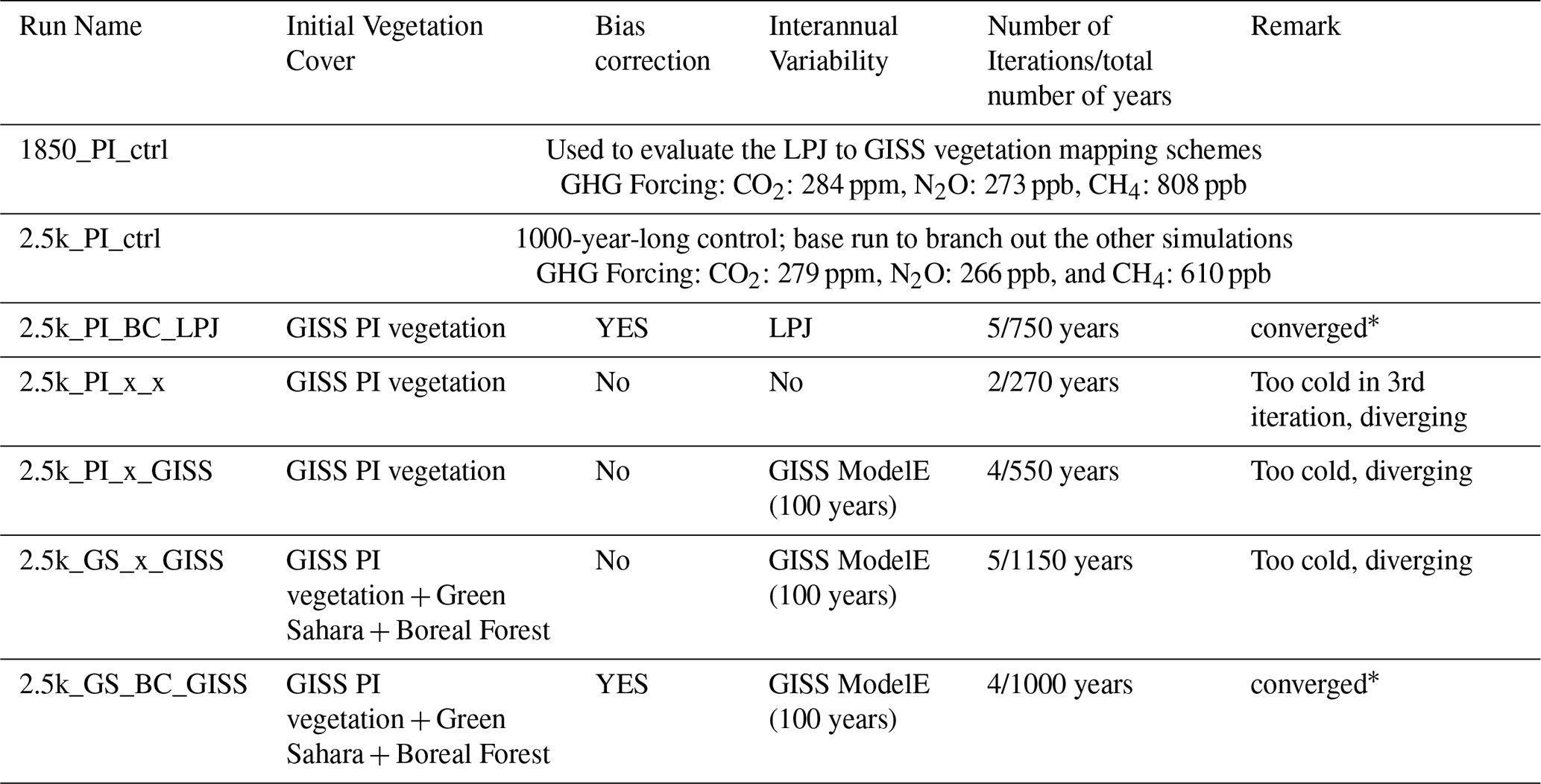
^* Convergence means the final iteration model simulation has a similar climatology with the previous iteration, whereas divergence means the model is drifting away from the expected states.

3.1 Evaluation & Validation of LPJ-GISS Mapping Methodologies

We used the standard present-day land cover boundary conditions described for ModelE2.1 (Kelley et al., 2020) for the initial 0th-order iteration of the pre-industrial and 2.5 ka control climate simulations. This land cover dataset is based on satellite observations (Gao et al., 2008; Myneni et al., 2002; Tian et al., 2002a, b; Yang et al., 2006) from the Moderate Resolution Imaging Spectroradiometer (MODIS), with leaf area index (LAI) from the TRY database (Kattge et al., 2011), and vegetation height (Simard et al., 2011) from the Geoscience Laser Altimeter System (GLAS). Branches of the 2.5 ka run for green Sahara conditions are started using the linearly interpolated vegetations for 2.5 ka from the 6 ka vegetation distribution defined based on the PMIP4 protocol (Otto-Bliesner et al., 2017; Singh et al., 2023). These land cover boundary conditions are shown as the fractional coverage of 13 PFTs (including bare soils) (Figs. S1 and S2). In these figures, bare dark and bare bright are merged into a single bare soil fractional cover.

The ModelE2.1 pre-industrial (PI) control run initialized with the present-day land cover boundary condition is processed through the asynchronous coupling framework to evaluate the mapping scheme for converting LPJ PFTs to GISS (Ent) PFTs. We tested three sets of LPJ-to-GISS mapping schemes as required in the asynchronous coupling framework. Differences among the mapping schemes are described in Table S1. Three parallel control runs are performed for 100 years, each initialized with the vegetation distribution that corresponds to the corresponding mapping scheme and compared to the mean climate state of the parent PI control run.

Figure 2 Comparison of seasonal climate metrics between the PI control and different vegetation mapping. Top row shows the mean climatology for precipitation (mm d⁻¹; JJAS), surface air temperature (°C; ANN) and ground albedo (%; ANN) and rows 2 to 4 shows the differences in mean climate for the mappings LtoG_M0, LtoG_M1 and LtoG_M2, respectively. Stippling indicates the region over which change is not statistically significant at a 95 % confidence interval (Used the student's t-test).

The mapping schemes LtoG_M1 and LtoG_M2 (Table S1) generate a similar spatial structure of annual surface air temperature with broadly similar regional characteristics (Fig. 2). A shift towards colder climates of 2–3 °C in mean annual temperature over the higher latitudes of the Northern hemisphere is simulated when using the mapping scheme LtoG_M0, which is not present when using the other mapping schemes (LtoG_M1 and LtoG_M2). We selected forests into shrubs to match the missing PFTs in ModelE vegetation distributions based upon the tree height (Table S1). In these mapping schemes, the fraction of boreal tree PFTs assigned to cold shrubs depends on simulated tree height, which is, in turn, influenced by surface temperature (Bonan, 2008; Bonan et al., 1992; Li et al., 2013; Thomas and Rowntree, 1992). In the mapping LtoG_M0, the fractional cover of boreal tree PFTs was reduced significantly, leading to an increase in ground albedo (up to 10 %), which led to the model drifting towards comparatively colder climate conditions. When using the other two mapping schemes (LtoG_M1 and LtoG_M2) the assignment of boreal tree PFTs to shrub types is limited by a higher tree height threshold and partially because other PFTs (perennial grass) are substituted for cold shrubs. Regional patches of increased ground albedo and surface cooling over the higher latitudes of the Northern Hemisphere are also evident when using the LtoG_M1 and LtoG_M2 translation schemes.

Precipitation during the Northern Hemisphere summer monsoon season (JJAS; June–July–August–September) appears similar among the three mapping schemes, as the larger changes are confined to the equatorial regions. A drying pattern over Europe appears in all three translation schemes, but it is comparatively more substantial under LtoG_M0 and LtoG_M1 than LtoG_M2.

All translation schemes also lead to increased precipitation over equatorial South America. Annual mean river runoff for the Amazon River is simulated at 305, 297, and 308 km³ per month for LtoG_M0, LtoG_M1 and LtoG_M2, respectively, a slight improvement to the original Preindustrial (PI) run runoff of 280 km³ per month using the standard present-day land cover boundary condition. Compared to observations, ModelE2.1 shows a substantial deficit in Amazon River runoff in present-day simulations because of insufficient precipitation over the watershed (Fekete et al., 2001; Kelley et al., 2020).

Based on this evaluation of the different ways of translating LPJ PFTs to GISS PFTs, we found that LtoG_M2 was the scheme that simulates global precipitation and surface temperature most consistently with observations, and ground albedo that is closest to the standard pre-industrial boundary conditions dataset used usually used to drive ModelE. Figure 3 shows the difference in PFT cover fraction using LPJ-LMfire with the LtoG_M2 scheme compared to the standard ModelE boundary condition land cover data set for the late preindustrial time (PI; 1850 CE).

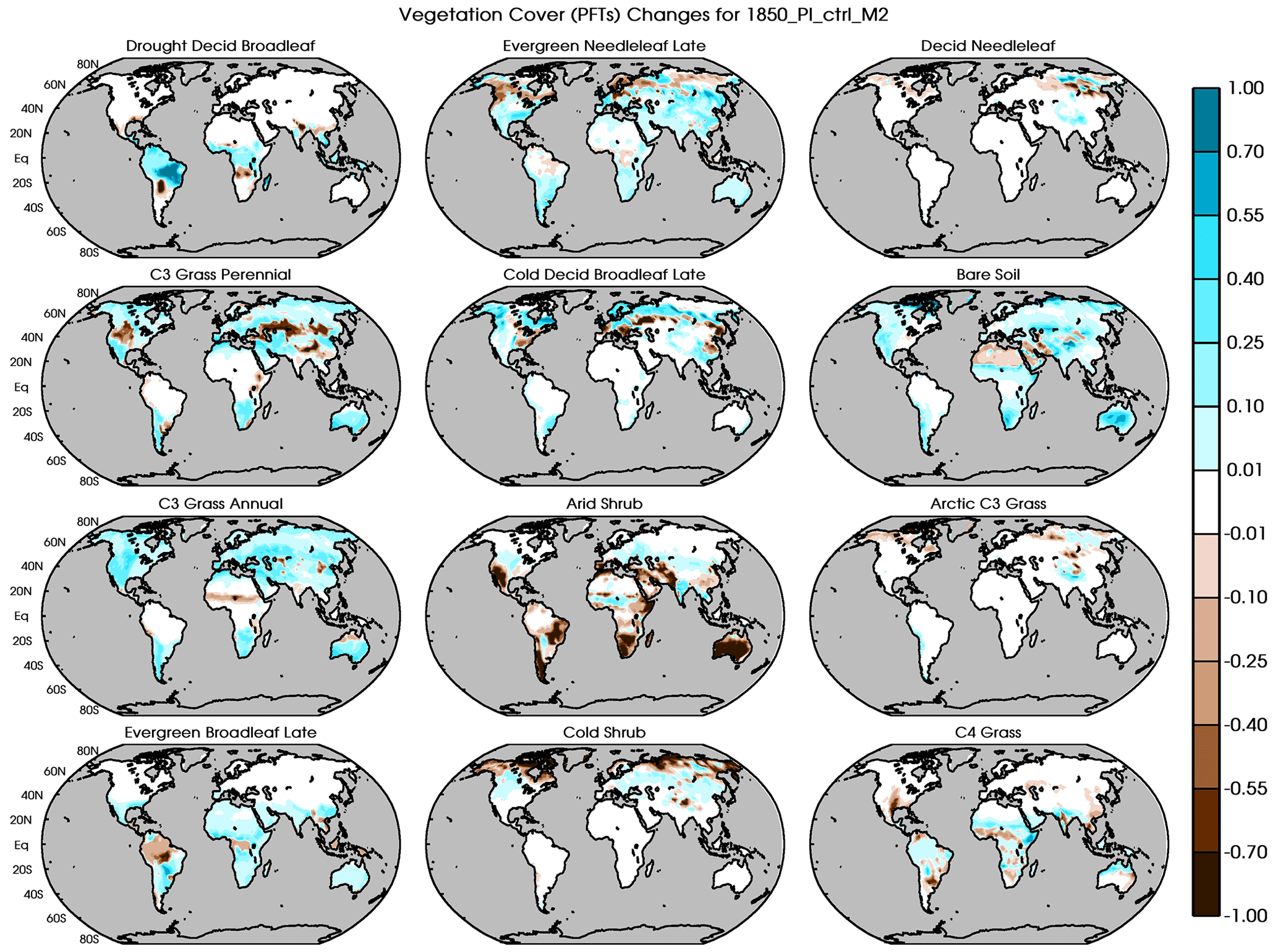
Figure 3 Differences between the LPJ-LMfire simulated vegetation distribution (PFTs and land cover type) and satellite-based land cover boundary conditions used in ModelE for the PI control period and the selected mapping schemes (LtoG_M2).

Compared to the ModelE standard land cover dataset for PI, LPJ-LMfire simulates increased extent and fraction of most trees (drought broadleaf, evergreen needleleaf, and evergreen broadleaf). Despite selecting a relatively high threshold for tree height to be classified as shrubs (up to 11 m for both arid and cold types) the simulated cover fraction of shrubs is low compared to the standard PI land cover dataset for ModelE. The coverage of both annual and perennial C₃ grasses is greater in LPJ-LMfire in extratropical and polar regions. Similarly, C₄ grasses, which are not present in cooler climates, shows greater coverage in LPJ-LMfire in equatorial regions. LPJ-LMfire simulates some vegetation cover in the Sahara and Arabian deserts while the standard PI boundary conditions dataset suggests that most of this region is bare soil.

3.2 Vegetation Cover Changes under various combinations

We chose a set of five model configurations (Table 2) to quantify the model bias and interannual variability in our asynchronous coupling framework for the 2.5 ka period. Figures S3, S4, S5, S6, and S7 show the spatial differences between prescribed land cover boundary conditions maps and land cover interactively simulated by our LPJ-LMfire-ModelE coupled model, which is henceforth referred to as the “coupled model system”. These land cover difference maps are shown for each of the different model configurations described above, following the final iteration of the asynchronous coupling when the coupled model system is assumed to be either equilibrated or the process was truncated due to instability (Table 2). Figures S3, S4, and S5 show the changes in the land cover from the default ModelE land cover boundary conditions map for PI (Fig. S1); Figs. S6 and S7 show the differences calculated from the modified vegetation following the PMIP4 protocols (Fig. S2).

Across all configurations, most of the tree PFTs show an increase in cover in the coupled model system relative to the prescribed land cover maps. However, in simulations where bias correction to the climate model was not applied, deciduous needleleaf tree cover is reduced in the high latitudes of the Northern Hemisphere (2.5k_PI_x_x, 2.5k_ PI_ x_GISS and 2.5k_GS_x_GISS) and this, in turn, has a substantial impact on regional climate. The coupled model system simulates increased annual and perennial C₃ grass cover across all configurations relative to the prescribed maps, while the Arctic C₃ grass shows a mixed regional response. Increased C₄ grass cover is mostly confined to the equatorial region and Southern Hemisphere; over the Northern Hemisphere C₄ grass cover decreases, irrespective of the inclusion and exclusion of interannual variability or bias correction. As discussed previously, the extent of arid and cold shrubs is reduced significantly in the coupled model system relative to the prescribed maps, even when the threshold height to separate trees from shrubs was set at a relatively tall limit of 11 m. A similar reduction in shrub cover relative to the land cover map used to initialize the simulation vegetation distributions is also simulated under all configurations.

In Figs. 4 and 5 we present heatmap-type diagrams of the mean land cover fraction over selected regions to demonstrate and understand the pattern of change in vegetation distribution simulated by the coupled model system. These figures depict changes in land cover under the different asynchronous coupling experimental configurations used in this study. Vegetation fraction change is averaged over northern Asia (NAS) (Fig. 4) and eastern Africa (Fig. 5; see Fig. 13 for the region boundaries; NAS: magenta; EAF: blue). Deciduous needleleaf tree cover over northern Asia (60–77° N, 70–135° E) is replaced by bare soil in all experimental configurations where bias correction of the climate model output was not applied. A similar disappearance of evergreen needleleaf late-successional forests, as well as a quick disappearance (within the first iteration) of cold shrubs, was also noticed. This suggests that, in the absence of bias correction, the model's drift towards colder conditions strongly influences vegetation growth in subsequent iterations over higher latitudes, which is inconsistent with the standard land cover boundary condition dataset used with ModelE (Kelley et al., 2020). On the other hand, when bias correction is applied along with interannual variability from either model (2.5K_PI_BC_LPJ and 2.5K_GS_BC_GISS), boreal forests are present in the northern Asia region along with cold shrubs and grasses.

Figure 4 Area average of fractional land cover over Northern Asia region (60–77° N, 70–135° E) under the range of experimental configurations used in this study.

Figure 5 Same as Fig. 4, but for Eastern Africa (0–18° N, 25–46° E).

Over eastern Africa (EAF: 0–18° N, 25–46° E) the impact of bias correction is less important than over the high latitudes of the Northern Hemisphere. The presence of broadleaf tree PFTs (drought broadleaf and evergreen broadleaf) and C₄ grasses is consistent across all the experimental configurations used. However, the cover fraction of arid shrubs decreased substantially, associated with a slight increase in the bare soil fraction.

4 Comparison with paleoclimate-proxy records for 2.5 ka

To evaluate the coupled model system's skill in representing past climate, we compared our simulations for 2.5 ka with multiproxy temperature reconstructions and speleothem-based oxygen isotope records.

4.1 Comparisons with reconstructed temperature

Kaufman et al. (2020) used five different statistical methods to reconstruct temperature at 1319 globally distributed sites covering part or all of Holocene from a range of proxy types. For each method, a 500-member ensemble of plausible reconstructions was presented. For comparison with our model output, we extracted temperature anomalies for 2.5 ka (relative to the value reconstructed for the late preindustrial Holocene) from the ensemble reconstructions, which then binned into six latitude bands between the North and South Poles (each 30° wide). We computed the mean and median zonal anomaly using all 500 estimates of mean surface temperature (MST) over each band for each of the five methodologies (total 2500), along with the 5–95 percentile interval to represent uncertainty/variability among the sites in each zone and across reconstruction methods (black bar in Fig. 6) as suggested by Kaufman et al. (2020).

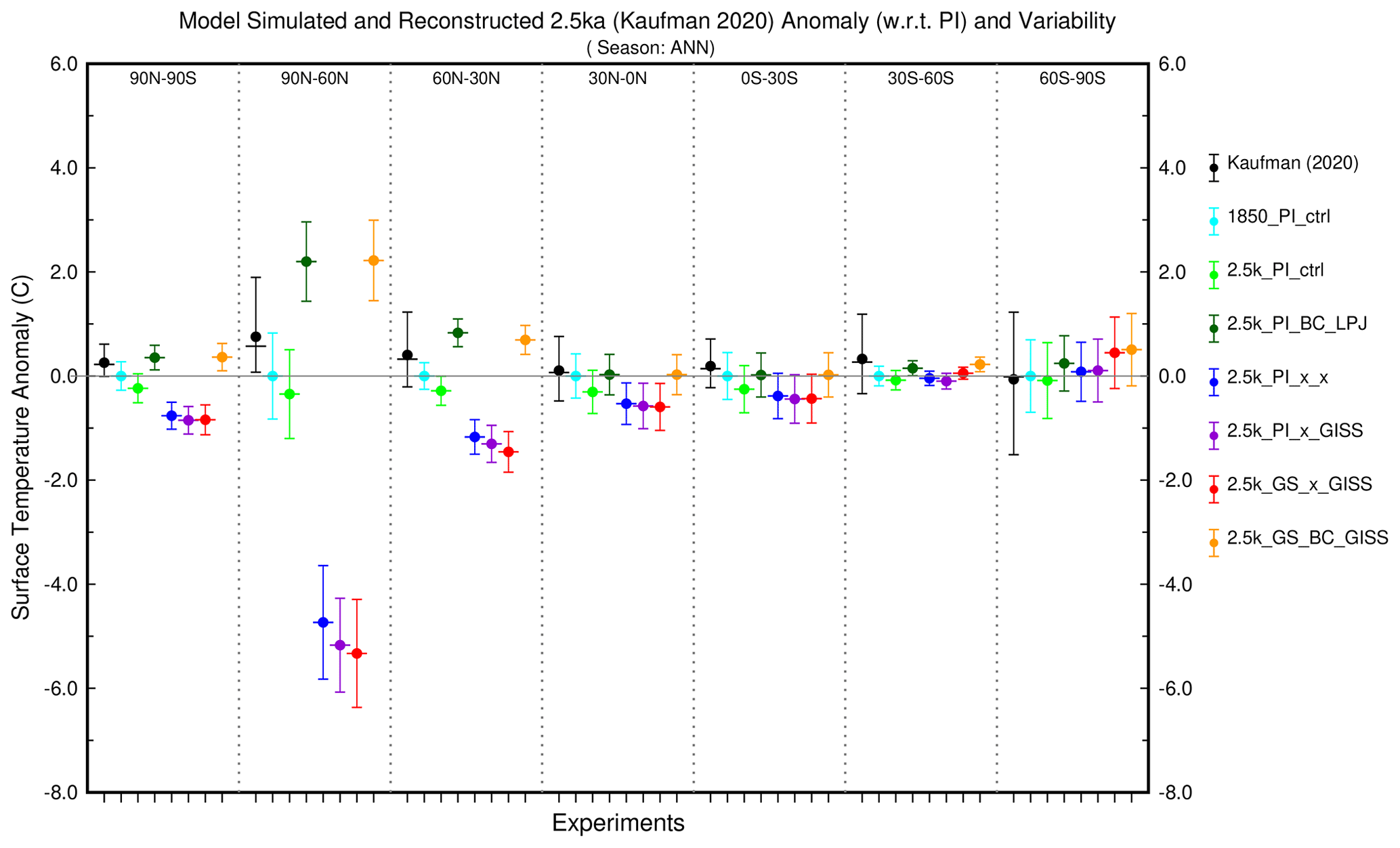
Figure 6 Comparison of model-simulated annual surface temperature anomalies and interannual variability for 2.5 ka (with LPJ-LMfire vegetation) against independent proxy-based temperature reconstructions (black, Kaufman et al., 2020). Mean (circle), median (line) along with the 5–95 percentile range as variability bars (whiskers) and different colors that represent the final iteration of our different experiments.

Figure 6 shows that the 2.5 ka control simulation with present-day vegetation is comparable to pre-industrial conditions (1850_PI_ctrl), exhibiting a slightly cooler climate. In contrast, proxy-based surface temperature reconstructions (Kaufman et al., 2020) indicate slightly warmer conditions at the global mean as well as across most latitude bands, except the far south (60–90° S). Applying bias correction allows the model to reproduce the same anomaly sign as the reconstruction, with minimal global (90° N–90° S) mean bias relative to the proxy data (2.5k_PI_BC_LPJ and 2.5k_GS_BC_GISS). Although the magnitude of warming remains higher at the northern hemisphere high latitudes, this framework demonstrates the improved capability of the model to reproduce reconstructions through the incorporation of biogeophysical effects of past vegetation by adopting a bias correction. Model simulations where bias correction was not applied show colder conditions than the reconstructions globally and in the Northern Hemisphere. These differences between model and proxy are very large in the high latitudes of the Northern Hemisphere and statistically significant throughout the extra-tropics. In the Southern Hemisphere, the differences between model and proxy reconstructions are smaller and insignificant, and there is less difference between simulations with and without bias correction. It should be noted that the larger uncertainty in reconstructed temperature over the southern polar band is due to a noticeably lower number of available proxy records (157 records; Kaufman et al., 2020).

4.2 Comparisons with speleothem oxygen isotope ratios

The isotopic composition of oxygen in water, expressed as the ratio of ¹⁸O to ¹⁶O serves as a fundamental tracer for investigating changes in the hydrological cycle. This ratio is highly sensitive to regional climate conditions and to the processes that regulate the hydrological cycle, such as temperature, precipitation, and evaporation. ModelE2.1 includes a representation of the stable water isotopologues as passive tracers and the isotopic composition of precipitation can be diagnosed from the model output (Aleinov and Schmidt, 2006; LeGrande and Schmidt, 2006; Schmidt, 1998). We compared the simulated mean annual isotopic composition of precipitation (δ¹⁸O_p) with oxygen isotope records from the Speleothem Isotope Synthesis and Analysis (SISAL) version 2 database (Comas-Bru et al., 2020). Using the published chronologies for each speleothem record we extracted all samples dated between 3–2 ka, which resulted in 163 measurements from 111 sites. Depending on their mineralogy (i.e., calcite or aragonite), the mean δ¹⁸O values (VPDB) were converted to their drip water equivalents that could be compared to simulated δ¹⁸O_p (VSMOW) (Comas-Bru et al., 2020). We used simulated mean surface air temperature obtained from the grid points nearest each cave site to estimate the cave temperature required to convert mineral δ¹⁸O to an equivalent the drip water value. For each of our model experiments, we extracted simulated δ¹⁸O_p nearest to each cave site and compared it with the estimated drip-water δ¹⁸O.

Overall, the mean δ¹⁸O_p spatial distribution in all 2.5 ka simulations is in excellent agreement with the proxies, showing better pattern correlations (r_pat) than 0.83 (Fig. 7), with the 2.5k_PI_x_x iteration marginally showing the highest skill (i.e., r_pat = 0.85 and RMSE = 1.90; shown in Fig. S8). For comparison, the worst simulation using this metric, 2.5k_GS_BC_GISS, is almost as equally skillful (r_pat=0.84 and RMSE = 1.92; Fig. S8), demonstrating that none of the different configurations we presented here were significantly different.

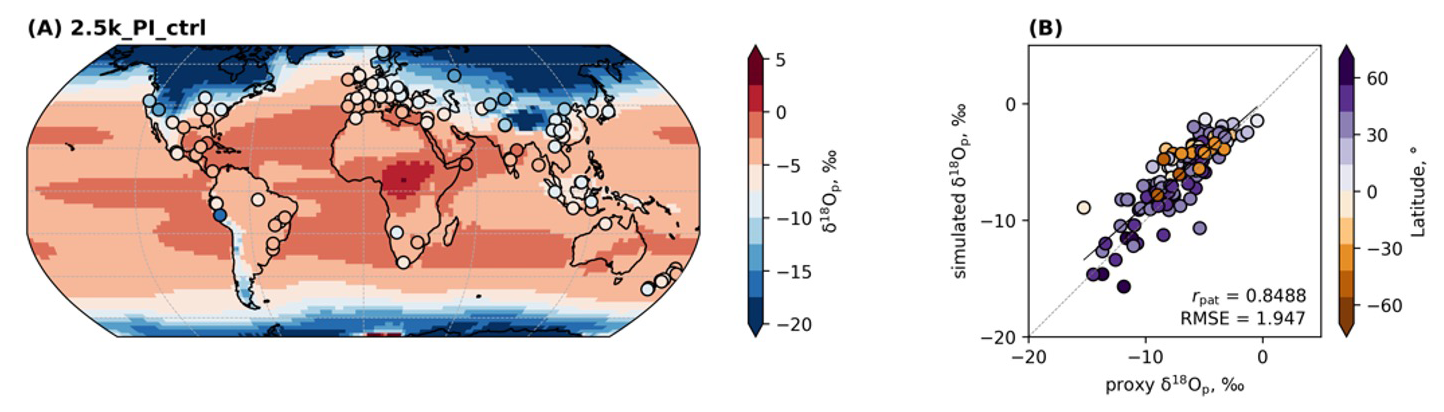
Figure 7 Comparison of simulated δ¹⁸O_p with speleothem δ¹⁸O. (A) Global distribution (70° S–70° N) of simulated δ¹⁸O_p (background) and speleothem δ¹⁸O (circles), converted to their drip water equivalents (see main text) for the 2.5k_PI_ctrl simulation. (B) Scatterplots between simulated and proxy δ¹⁸O_p. Black line represents the least squares regression fits to data points, while the gray dashed line represents the 1 : 1 line. r_pat and RMSE are reported in the lower right corner of the scatterplot. For comparison against each model experiment, see Fig. S8.

Regionally, we similarly found that most simulations show no significant deviation with each other (Figs. 8, 9). We note, however, that over Europe (Fig. 9E), variability may be explained by the observed change in magnitude on both SAT and summer precipitation among simulations (further sections). Over India and Central Asia (Fig. 9F), simulations with bias correction show lower correlation and higher RMSE values compared to other models against proxy δ¹⁸O_p. This is likely related to the observed increase in mean summer precipitation over this region that was not reflected in the proxy sites.

Figure 8 Demarcation of geographical regions described in the main text. Labels A to J correspond to the respective Taylor diagram plots in Fig. 9.

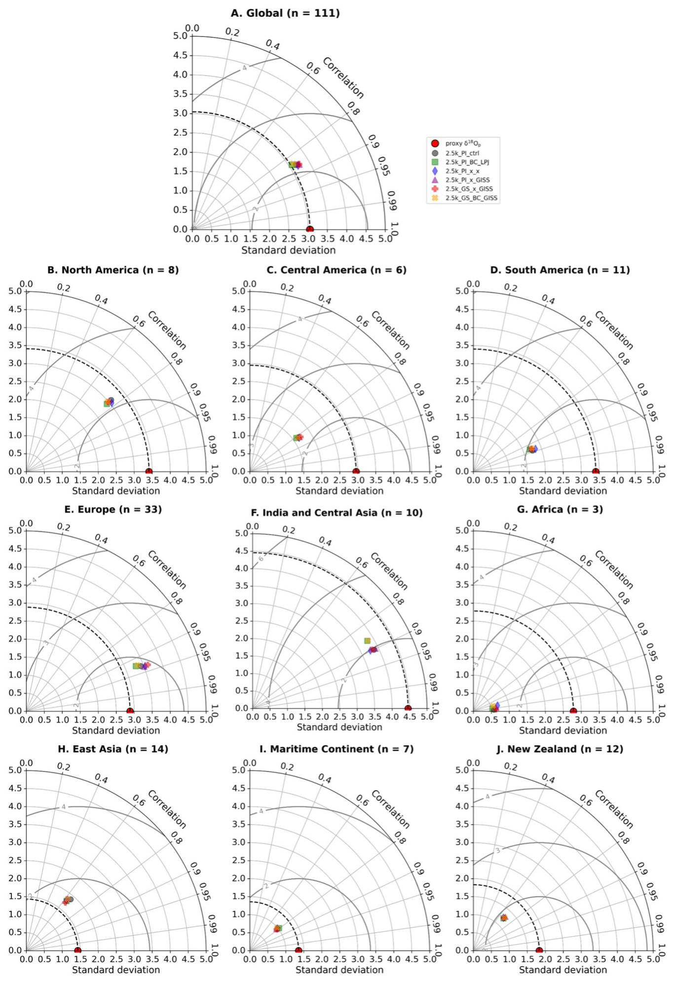
Figure 9 Taylor diagrams showing the r, SD and RMSE values between the proxy-derived and simulated δ¹⁸O_p for each 2.5 k iteration globally (A) and at each subregion (B–J). The sub-regions are shown on the map in Fig. 8.

Compared to proxy δ¹⁸O_p, simulations over certain regions show better agreement. Europe, which is the most densely sampled region, show the best agreement with the proxies (i.e., high correlation, closest to the reference point, Fig. 9E), and with the 2.5k_PI_x_GISS iteration best capturing the spatial δ¹⁸O_p pattern (i.e., r_pat = 0.94 and RMSE = 1.26). In contrast, simulations over Central America, South America and Africa show the least skill where the magnitude of δ¹⁸O_p change is consistently underestimated (i.e., moderate to high correlation but farthest away from the reference point). This may largely be due to inadequate sampling in these regions, especially for Africa, and/or both precipitation and SAT influencing δ¹⁸O may be underestimated at these proxy locations, resulting in a generally muted δ¹⁸O response across simulations. Cave-specific factors that alter speleothem δ¹⁸O, for example, groundwater mixing or fractionation (Baker et al., 2019; Hartmann and Baker, 2017; Lachniet, 2009) are also not effectively reproduced in the models, contributing to the proxy-model mismatch. Regions where the largest simulated SAT, precipitation, and δ¹⁸O_p change relative to the 2.5k_PI_ctrl are observed, such as northern Africa, the Amazon basin and Siberia, are not adequately represented by reconstructions, highlighting the need to expand the proxy network to marine-based records and polar regions over the period of interest to capture the full range of isotopic variation.

5 Global climate response

To evaluate the spatial features of the equilibrium climate simulated by ModelE, we analyzed the last 100 years of the final iteration of each coupled model system experimental configuration. We aimed to understand the biogeophysical feedback due to vegetation cover changes as well as the role of model configuration on climate. Figure 10 shows surface albedo (%) for ModelE in its initial PI state, and differences between this initial state and simulated albedo for 2.5 ka using the coupled model system. We used student's t-tests to estimate if the albedo differences were statistically significant at the 95 % confidence level. The coupled model system shows substantial vegetation cover change over the high latitudes of the Northern Hemisphere. As expected, most of the significant changes occur over land, while changes in albedo over the oceans are largely insignificant. The spatial pattern of albedo change differs between simulations where bias correction was applied (2.5k_PI_BC_LPJ and 2.5k_GS_BC_GISS) and those where it was not (2.5k_PI_x_x, 2.5k_PI_x_GISS, and 2.5k_GS_x_GISS). Albedo over the high latitudes of the Northern Hemisphere decreases up to 10 % caused by increased tree cover fraction (deciduous needleleaf and evergreen needleleaf) in the coupled model system relative to standard PI land cover dataset.

Figure 10 Annual mean (top left; 2.5k_PI_ctrl) and change (all other panels) of surface albedo (%) for the final iteration of various experiment configurations listed in Table 2. Stippling indicates the region over which change is not statistically significant at a 95 % confidence level (using the student's t-test).

This increased tree cover fraction subsequently absorbs more incoming solar radiation and raises surface temperature by 2–4 °C over high latitude regions compared to the control run (Fig. 11 top-right and bottom-right panels). In experiments where bias correction was not applied (2.5k_PI_x_x, 2.5k_PI_x_GISS and 2.5k_GS_x_GISS), the relatively cold conditions simulated by the coupled model system shows an opposite albedo-vegetation response (>3 °C cooling over Northern Hemisphere high latitudes). This drift towards a colder climate in the absence of bias correction resulted in the continuous formation of sea ice that ultimately reaches the (shallow) seabed, effectively creating land ice and eliminating the ocean from the grid cell. In coupled model system experiments without bias correction, we terminated the iterative processes when this freezing of the ocean to the seabed occurred, because this condition caused the model to crash (2.5k_PI_x_x, 2.5k_PI_x_GISS, and 2.5k_GS_x_GISS).

Figure 11 Same as Fig. 10 for Surface air temperature (°C) mean and change on an annual scale (ANN season).

At lower latitudes, albedo tends to show decreases relative to the standard boundary conditions in all experiments, particularly over the forested areas of the equatorial regions and temperate latitudes of the Northern Hemisphere. Over northern Africa and the Indian subcontinent, changes in both albedo and surface temperature are more mixed. Albedo change in central and northern Africa are driven by a reduction in the area occupied by shrubs and an increase in bare soil fraction. This pattern of increased albedo is more prevalent in simulations that were initialized with Green Sahara land cover boundary conditions.

In experiments that were initialized with “Green Sahara” land cover boundary conditions where interannual variability from GISS ModelE is included with and without adopting the bias correction, comparison of the surface temperature response between simulations with (2.5k_GS_x_GISS; Fig. 11, bottom-left) and without bias correction (2.5k_GS_BC_GISS; Fig. 11, bottom-right) reveal the significance of bias correction for the asynchronous coupling process. Broadly, we can observe that bias correction induces a warming of 0.7–0.8 °C, and exclusion leads to a cooling of 0.9–1.1 °C, at the global scale, predominantly over the northern hemisphere land regions.

Precipitation change across the model configurations is shown for Northern Hemisphere summer (JJAS) at global scale in Fig. 12. The significance of bias correction is noticeable over the high latitudes of the Northern Hemisphere. Simulations with bias correction (2.5k_PI_ BC_LPJ, 2.5k_GS_BC_GISS) lead to an increase in JJAS season precipitation relative to the initial boundary conditions, while those experiments without bias correction (2.5k_PI_x_x, 2.5k_PI_x_GISS) show reductions in precipitation. Reductions in precipitation relative to initial conditions are visible in Europe in all configurations and are greater in experiments where bias correction was not applied. Another common feature among the experiments was the variable spatial pattern of JJAS precipitation change over tropical regions. All configurations showed increased precipitation over south and east Asia. Over the Nile headwaters in East Africa (Melesse et al., 2011) precipitation increased, particularly in those experiments where bias correction was applied. Interestingly, increased Northern Hemisphere summer monsoon season (JJAS) precipitation over the Asian continent was simulated across all configurations. In contrast, only a marginal northward procession of ITCZ over tropical Africa was simulated.

Figure 12 Same as Fig. 10 for precipitation (mm d⁻¹) mean and change for the JJAS season.

Regional climate

The spatial pattern of changes in climatic features for 2.5 ka using our coupled model system shows several prominent and robust regional signatures of climate change. We selected nine regions over land (Fig. 13; Table 3) to analyze regional temperature and precipitation changes in our simulations. Area-averaged time-series anomalies with respect to the 2.5 ka control run (2.5k_PI_ctrl) for the various experiments performed are calculated for these different regions.

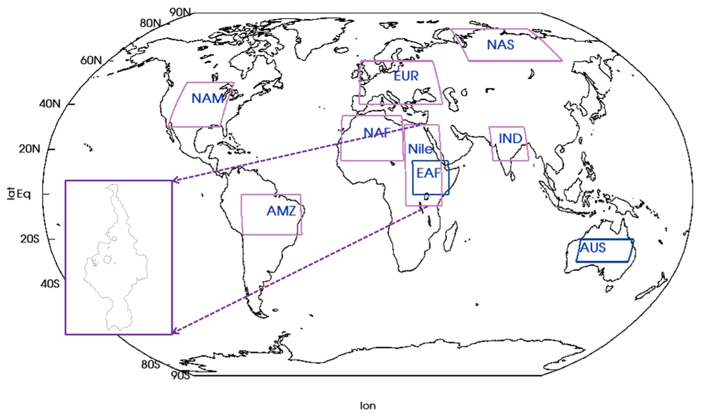
Figure 13 Boundaries for the regions used for regional analysis. The inset map shows the Nile River basin in high resolution, which is superimposed upon the ModelE resolution to generate the grid-specific weights for the Nile River basin. The EAF and AUS regions are used in Figs. 4, 5 and 15.

Table 3 Region details including the boundary coordinates for all the regions.

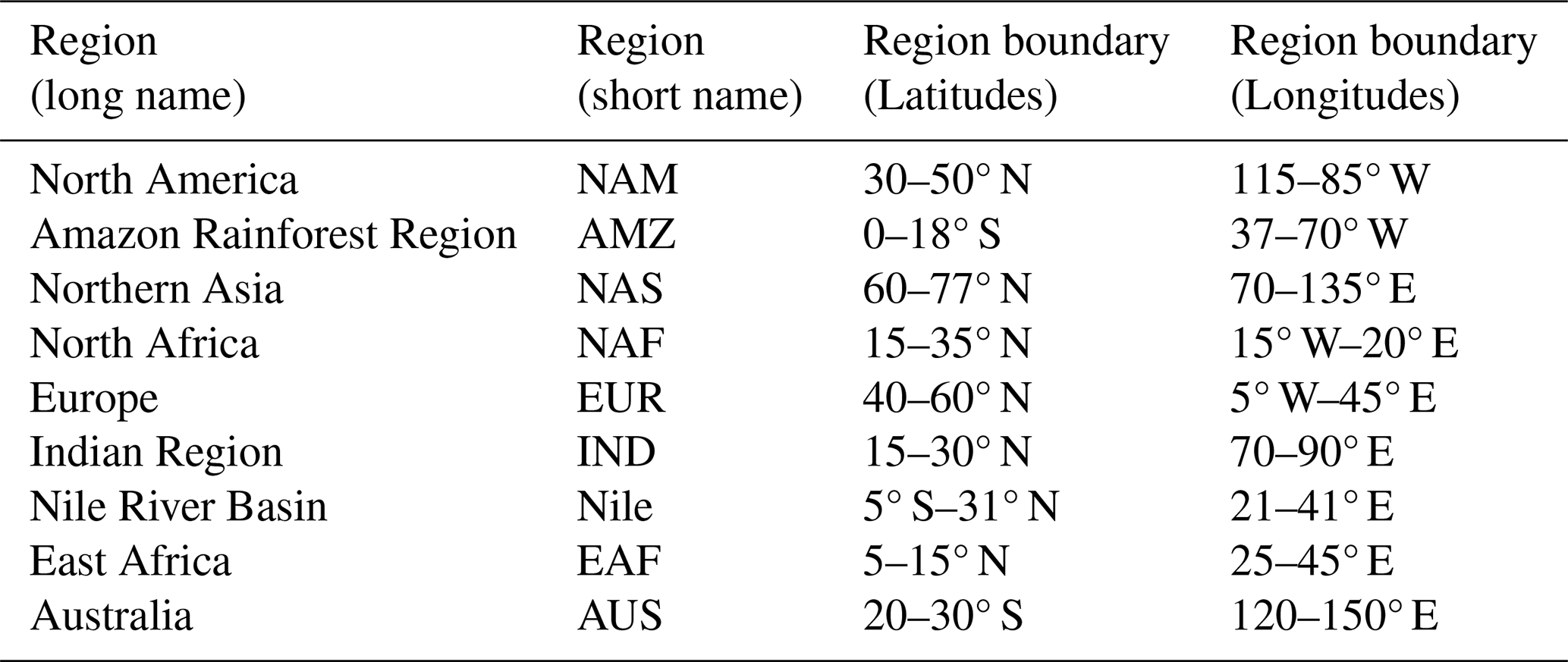
Figure 14 shows box-and-whisker plots of mean and median annual surface temperature (top) and JJAS seasonal precipitation (bottom) change, as well as the 5–95 percentile range (interannual variability) along with the upper and lower quartiles (25th and 75th percentiles) of the anomaly time series for each region. As suggested from the global analyses of spatial patterns, the shift towards relatively warmer or colder climate as a result of applying bias correction is evident. Bias correction leads to a pronounced warming over northern Asia (NAS region) of 3–4 °C, while without bias correction this region cools by 5–6 °C. The partition between experiments with and without bias correction is also apparent over selected regions of the mid-latitudes between 35–60° N (NAS and EUR).

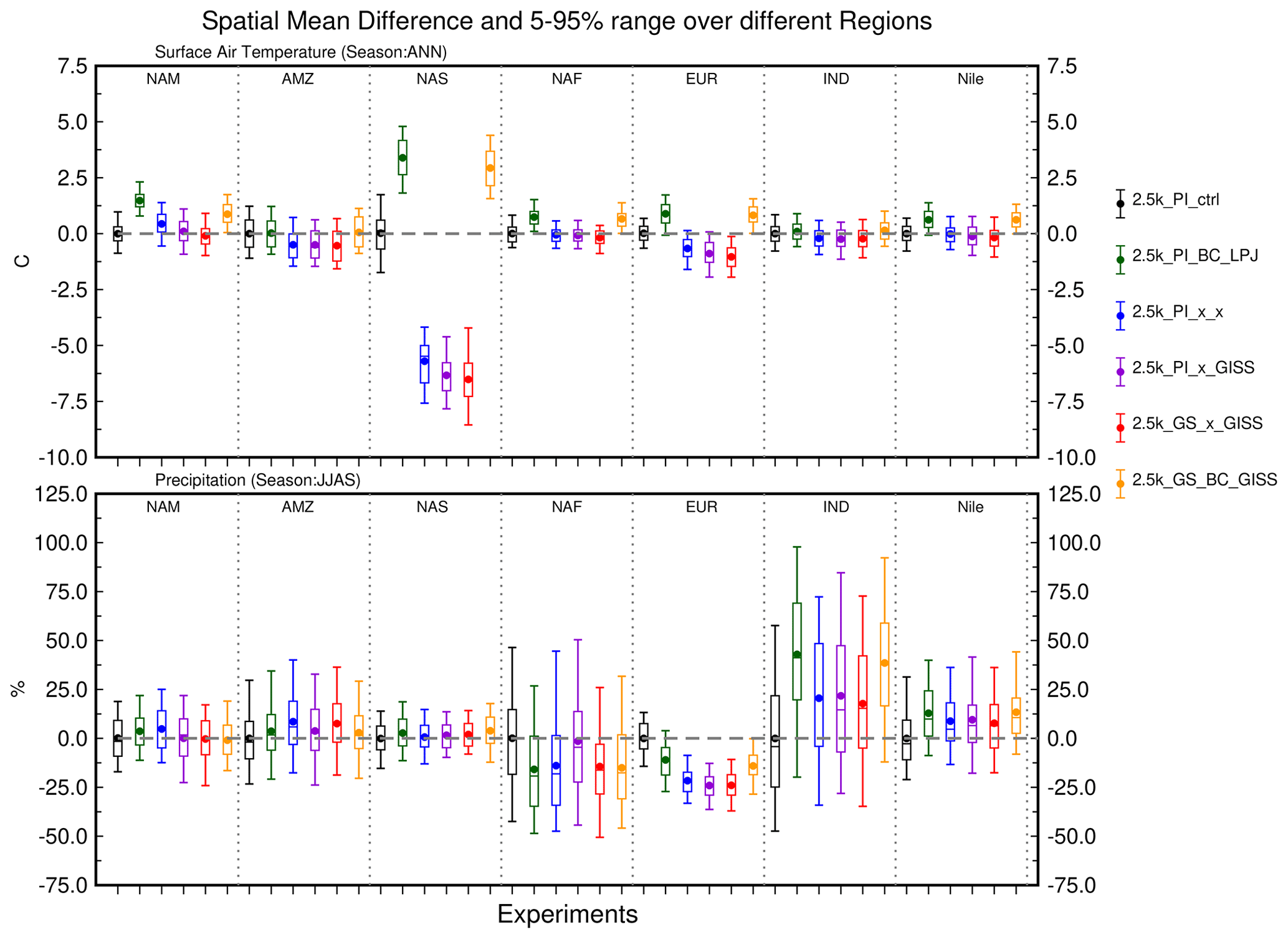
Figure 14 Regional change in surface air temperature (top panel, °C, annual mean) and precipitation (bottom panel, %, JJAS) for the various simulations with respect to the 2.5 ka control run (2.5k_PI_ctrl). Regions as listed in Table 3.

Except for northern Asia (NAS), all regions show approximately similar interannual variability in mean annual surface temperature. In northern Asia interannual variability is greater, especially in simulations where bias correction was not applied. Our results show that interannual variability in summer temperature in northern Asia is sensitive to changes in land cover, with greater variability in simulations where bias correction was not applied.

Simulated 2.5 ka precipitation for the Northern Hemisphere summer (JJAS) shows substantial changes in mean state relative to the 2.5 ka control with PI vegetations, particularly for the tropical regions of northern Africa, India, and the Nile basin (Fig. 14, bottom panel). Interannual variability in precipitation is comparable to the initial control run (black line). However, the magnitude of variability differs across the regions; it is more prominent in tropical regions than in the extra tropics. An increase in mean precipitation on the order of 20 %–30 % without bias correction and up to 40 % with bias correction is simulated in JJAS season precipitation for the Indian summer monsoon region (IND) and it is in a range of 10 %–25 % increase over the Nile basin region. A drying pattern over Europe (EUR) ranges from 10 %–25 % and is consistent for all the simulations; a greater decrease in European precipitation was simulated when bias correction is not adopted. A similar drying pattern was also simulated over the North America (NAM) and northern Africa (NAF) regions. The relatively small magnitude of interannual variability in precipitation over Europe and North America suggests that our model does not produce high variability across these regions and that it is not sensitive to the different experimental configurations. Despite the large changes in both mean state and variability in temperature, precipitation over northern Asia (NAS) changes little from the control state and across simulations. In the Amazon region (AMZ), precipitation changes were small and not significantly different between simulations. Without bias correction, the coupled model system suggests a modest increase in mean seasonal precipitation of up to 10 %. We also noticed a similar response of slightly increased precipitation in Southern Hemisphere summer (DJF) over Australia (not shown here).

We further investigated the way our experiments influenced the seasonal cycle of temperature and precipitation over the regions discussed above. Our results show that the seasonal cycle of surface temperature is broadly similar across experiments for all the equatorial regions except the Amazon (AMZ) region, where surface temperature is reduced by 0.5 °C in experiments where bias correction was not applied (Fig. S9). Over the northern Asia (NAS) region, we see a considerable difference in the seasonal cycle of temperature of 5–15 °C between runs with and without bias correction. The seasonal cycle of temperature in the 2.5 ka control (2.5k_PI_ctrl) simulation over NAS is intermediate to the experiments but tracks closer to the simulations where bias correction was applied, particularly in Northern Hemisphere winter, where, as noted above, simulations without bias correction result in very cold conditions in this region.

Figure 15 Seasonality of precipitation averaged over the selected regions for the final iteration of each experiment listed in Table 2.

Compared to temperature, the seasonal cycle of precipitation shows greater differences among simulations over several of the regions (Fig. 15). An increase of 2–3 mm d⁻¹ over the Indian region (IND) is simulated during the Indian Summer Monsoon months (JJAS) when using LPJ-LMfire-generated land cover for both types of experiments (with and without bias correction), with the bias-corrected simulations showing a larger increase in precipitation than the non-bias-corrected ones. When bias correction is applied, the seasonal peak of precipitation shifts from July to August. Over Europe, we observe a decrease of up to 0.5 mm d⁻¹ in summer precipitation relative to the control simulation in all simulations that use the LPJ-LMfire PFTs. Precipitation decreases even more when the bias correction was not applied. The North Africa region (NAF) also shows a slight decrease in precipitation relative to the control over most of the seasonal cycle, while in North America (NAM) we see an increase in precipitation outside of the JJAS summer months. The Amazon rainforest region (AMZ) shows no change in the seasonal cycle of precipitation in all experiments. The Nile River basin (Nile) and Australian (AUS) regions also show small increases in precipitation relative to the control in their respective monsoon seasons (JJAS and DJF). Overall, the changes in annual precipitation cycle (increases or decreases) over the studied regions are primarily driven by both the pole-equator thermal gradients in the various experiments, as well as the biogeophysical effects associated with regional vegetation changes over these regions (e.g. Indian Summer monsoon, North American and European region) (Pausata et al., 2016; Tiwari et al., 2023; Singh et al., 2023).

6 Discussion and Conclusions

Here we presented a generalized technical framework for asynchronously coupling a climate model (NASA GISS ModelE2.1) with a dynamic vegetation model (LPJ-LMfire), i.e., the “coupled model system”, and demonstrate its skill in reconstructing climate in the late preindustrial Holocene and for 2.5 ka. We examined the role of bias and interannual variability corrections in this process, and showed how they influence simulated land cover and climate. We demonstrated the importance of considering such metrics in such a framework in our experimental design and global and regional scale analyses. We performed a detailed evaluation and comparison of the climate simulated by the coupled model system with reconstructions of air temperature (Kaufman et al., 2020) and the isotopic composition of precipitation (δ¹⁸O_p) based on speleothems (Comas-Bru et al., 2020). Similarly to previous studies that used asynchronous coupling to simulate regional and global paleoclimate (Claussen, 2009; Kjellström et al., 2009; de Noblet et al., 1996; Strandberg et al., 2011, 2014b; Texier et al., 1997; Velasquez et al., 2021), we assessed the influence of the biogeophysical feedback between land and atmosphere.

Our results demonstrate the pronounced influence of including bias correction when passing simulated climate to the land surface model. To correct biases inherent in the climate model, in selected experiments we passed climate anomalies relative to a control simulation to the land model that were added to a standard baseline climatology based on contemporary observations. In simulations without this bias correction, raw simulated climate was passed directly from ModelE to LPJ-LMfire. Where bias correction was applied ModelE drifts towards warmer climate; simulations without bias correction drift towards colder climate. This effect was especially apparent in the high latitudes of the Northern Hemisphere, particularly over Asia. With bias correction, high latitude vegetation is dominated by tree plant functional types, while without it, cold shrubs and arctic grasses are the predominant form of land cover. These results are characteristic of the well-known vegetation-albedo feedback that is important at high latitudes (Charney et al., 1977; Charney, 1975; Doughty et al., 2012, 2018; Pang et al., 2022; Stocker et al., 2013; Swann et al., 2010; Zeng et al., 2021).

The effects of bias correction on precipitation were less apparent and confined to regional scale. We simulated a greater Indian summer monsoon season (JJAS) precipitation with bias correction (>1 mm d⁻¹), and a nominal increase of ∼ 0.5 mm d⁻¹ across east China, Africa, and the North American monsoon region. In other regions, the patterns of precipitation change were similar across all experiments except for Europe where drier conditions are simulated in summer (up to −1 mm d⁻¹) in simulations where bias correction was not applied.

The high latitudes of the Northern Hemisphere were also the region with the largest disagreement between model and independent, multi-proxy temperature reconstructions. These comparisons also highlighted the important role of bias correction; experiments with correction were much more similar to reconstructions than those without. Simulations of the isotopic composition of precipitation (δ¹⁸O_p) shows an excellent agreement with speleothem records with a pattern correlation greater than 0.8. However, the difference in the magnitude of model simulated δ¹⁸O_p from proxies over various regions indicates an underestimation of relationship between surface temperature and δ¹⁸O_p variability (Henderson et al., 2006; Kurita et al., 2004). A global evaluation of model skill is hindered by the difference in the number of independent paleoclimate reconstructions available for different regions, particularly in north Asia where we see the greatest sensitivity of the coupled model system to the experimental setup. When examining modeled and reconstructed δ¹⁸O_p, in Europe, which is the region with the greatest number of records, we see a robust pattern correlation with lower RMS values as compared to other regions.

In this study, we confirmed the importance of the land surface for simulating paleoclimate, even for the late Holocene where land surface conditions were not as different from present as they were during, e.g., the last glacial cycle or even mid-Holocene (6 ka). We demonstrated that asynchronous coupling can be a computationally inexpensive way of capturing land-atmosphere feedbacks and improving the fidelity of the simulated climate. We noted that correcting bias present in the climate model is essential for simulating climate that is consistent with independent reconstructions, particularly for the high latitudes of the Northern Hemisphere. Future work with the coupled model system will include quantification of the influence of major volcanic eruptions for regional and global paleoclimate and the influence of past climate on the dynamics of complex civilizations in prehistory.