A simple step heating approach for wall surface temperature estimation in the SOlar and LongWave Environmental Irradiance Geometry (SOLWEIG) model

The urban climate is highly influenced by its building geometry, material characteristics, street orientation and high fraction of impermeable surfaces. All of these influence the microclimate and the resulting outdoor thermal comfort. Mean radiant temperature (T_mrt) is often used as an estimator for heat exposure as it is one of the most important variables governing outdoor human thermal comfort on clear, calm and warm days. The highest values of T_mrt are commonly found in front of sunlit facades where a human is exposed to high levels of direct and reflected shortwave radiation from the sun, as well as high levels of longwave radiation emitted from surrounding sunlit walls. As a consequence, outdoor thermal comfort modelling requires accurate simulation of wall surface temperatures (T_s).

The aim of this study is to present a step heating approach for calculating wall T_s in the SOlar and LongWave Environmental Irradiance Geometry model (SOLWEIG) and quantify how it influences T_mrt. This method requires information on material characteristics, i.e. specific heat capacity, density, thermal conductivity, albedo and thickness of the outer layer of the wall, as well as radiation balance at the wall surface, and ambient air temperature. Simulated T_s is compared to observed T_s of two white walls (albedo = 0.5) in Gothenburg, Sweden; one wooden wall and one plaster brick wall. The simulations show high agreement with the 15 394 observations, with R²=0.93 and RMSE = 2.09 °C for the wooden wall and R²=0.94 and RMSE = 1.94 °C for the plaster brick wall. For the walls presented here, this new parameterization scheme results in differences in T_mrt of up to 2.5 °C compared to the previous version of SOLWEIG.

With this new approach, SOLWEIG can be used to evaluate the effect of building materials on outdoor thermal comfort. The speed and accuracy of this approach suggests that it also could be applied in other areas where T_s of walls are important, for example building energy models and urban energy balance models.

1 Introduction

The climate in urban areas is highly influenced by its building geometry (Muniz-Gäal et al., 2020; Nasrollahi et al., 2021; Xi et al., 2021), the orientation of streets (Ali-Toudert and Mayer, 2005), material characteristics (Santamouris and Yun, 2020; Adilkhanova et al., 2023; Battista et al., 2023), vegetation (Schibuola and Tambani, 2022; Stache et al., 2022) and the relatively high fraction of impermeable surfaces (Arnfield, 2003). Outdoor human thermal comfort is a consequence of the resulting microclimate. On clear, calm and warm days, the mean radiant temperature (T_mrt) is one of the most important factors in describing the outdoor thermal comfort of a human, and is used in many thermal comfort indices, e.g. the Physiological Equivalent Temperature (PET) (Mayer and Höppe, 1987; Höppe, 1999) and the Universal Thermal Climate Index (UTCI) (Blazejczyk et al., 2010). For UTCI, however, there are shortcomings when using it within the urban canopy layer because of its requirement of wind speed at 10 m above ground (Lee et al., 2025). T_mrt describes the radiant load that a human is exposed to, i.e. the exchange of short- and longwave radiation between the person and its surrounding radiative environment (Höppe, 1992; Thorsson et al., 2007). While spatial differences in air temperature (T_air) are usually very small in urban environments, the spatial differences in T_mrt between sunlit and shaded spaces can be up to 30 °C (Lau et al., 2015). For these reasons, many authors stress the importance of accurate modeling of T_mrt (Di Napoli et al., 2020; Gál and Kántor, 2020).

The shortwave radiation that a human is exposed to originates from the sun, with direct, diffuse and reflected components, whereas the longwave radiation originates from the sky, ground, vegetation and building surfaces, e.g. walls. There are numerous models to calculate T_mrt, including ENVI-met (Bruse and Fleer, 1998), RayMan (Matzarakis et al., 2007; Matzarakis et al., 2010), PALM-4U (Maronga et al., 2020) and The SOlar and LongWave Environmental Irradiance Geometry model (SOLWEIG) (Lindberg et al., 2008), all of which to some extent handle the above mentioned fluxes. Highest values of T_mrt are commonly found in front of sunlit walls (Lindberg et al., 2014) where a person would be exposed to high levels of direct and diffuse shortwave radiation as well as comparatively high amounts of reflected shortwave radiation off the wall (Wallenberg et al., 2020). Another highly influential aspect is if the wall is (or has recently been) sunlit, which increases its surface temperature (T_s) so that a person located close to the wall is exposed to higher emittance of longwave radiation.

There are several ways of estimating the T_s of a material. A common approach is with Fourier's law of diffusion (e.g. Simon, 2016; Resler et al., 2017), where the T_s of a material is calculated based on its energy balance that is estimated from heat conduction to or from the interior of the material, convection and radiative exposure. Here, thermal properties such as thermal conductivity, specific heat capacity and emissivity of the material are important, information that is not always easily accessible, especially in the interior of the walls. While this approach is accurate and dynamic, it is relatively time-consuming. Another faster approach is the force-restore method (Johnson et al., 1991). The force-restore approach uses two layers, one thin layer at the surface and one deeper layer, where the surface layer is exposed to gain or loss of energy and a deeper layer that restores or dampens the heating at the surface. Other approaches include empirical relationships, where T_s is observed and related to environmental variables, e.g. T_air or solar radiation, as in Bogren et al. (2000) and Lindberg et al. (2016). The empirical approach is only accurate for the specific material that it is calibrated on and requires logistically demanding field observations to incorporate new materials in modeling. Potentially, it is also only accurate for the time of measurements, e.g. season, used in the calibration. An additional approach that can be used to estimate the T_s of a material is step heating. Boué and Fournier (2009) used a step heating equation derived from the Dirac heat pulse to estimate T_s of materials. This is a straightforward approach, where the radiation balance at the surface of the material is used together with its thermal effusivity. Here, thermal effusivity (or thermal admittance (see Oke et al., 2017)) describes the ability of a material to absorb or return the thermal energy at its surface, for example between a wall surface and the ambient air.

As mentioned before, a common approach to estimate T_s is to use the concept of Fourier's law of diffusion and divide the wall into several layers and calculate its energy balance. The ENVI-met model uses three layers and calculates the temperature in seven nodes (Simon, 2016), whereas PALM-4U uses four layers and six nodes (Resler et al., 2017, 2021). Both of these models can simulate T_s with high accuracy. The TARGET model uses the force-restore method to estimate wall surface temperatures (Broadbent et al., 2019). Up to now, the SOLWEIG model uses the empirical approach described in Bogren et al. (2000) and Lindberg et al. (2016). The simulated T_s of ENVI-met (Simon, 2016) and PALM-4U (Resler et al., 2017, 2021) show high agreement with observations. The T_s of walls simulated with SOLWEIG has not been evaluated specifically. Gál and Kántor (2020) found that T_mrt simulated with SOLWEIG was underestimated in sunlit areas and overestimated in shaded areas, and that these offsets could be related to its wall surface temperature parameterization, i.e. the simple empirical approach (Bogren et al., 2000; Lindberg et al., 2016). Wallenberg et al. (2023a) also argued that the parameterization of wall surface temperatures in SOLWEIG could result in deviations in simulated emitted longwave radiation from building surfaces. In addition, SOLWEIG not being a full energy balance model, using simplified convection and conduction parameterizations, if included at all, should not be ignored.

The aim of this study is to present and evaluate a new step heating model approach for calculations of T_s of walls in the SOLWEIG model, and how this affects T_mrt.

2 Methods

2.1 Surface temperature parameterization

The basis of the T_s simulation is the step heating equation derived from the Dirac heat pulse as described in e.g. Boué and Fournier (2009):

$$\begin{array}{}\text{(1)}& T_{\mathrm{s}}={\displaystyle \frac{\mathrm{2}\mathit{\omega }}{e}}\sqrt{{\displaystyle \frac{t}{\mathit{\pi }}}}+T_{\mathrm{air}}\end{array}$$

where: ω is the heat flux density (W m⁻²), i.e. the sum of incoming and outgoing short- and longwave radiation of the wall; e is the thermal effusivity (W s^0.5 m⁻² K⁻¹) of the wall surface material, derived from:

$$\begin{array}{}\text{(2)}& e=\sqrt{\mathit{\lambda }\mathit{\rho }C}\end{array}$$

with λ being the thermal conductivity of the material, ρ is the density and C is the specific heat capacity. t is the characteristic time in seconds, as described below. T_air is the air temperature.

The wall surface is considered a semi-infinite solid that has a thickness L and extends infinitely in other directions. The time t in Eq. (1) is estimated from the characteristic time that describes the time it takes for the energy to propagate from the outdoor surface of the material to its approximately interior end, i.e. through the thickness L. The characteristic time is calculated according to Eq. (3) (Parker et al., 1961; Cape and Lehman, 1963; Xue et al., 1993; Philipp et al., 2020):

$$\begin{array}{}\text{(3)}& t={\displaystyle \frac{L^{\mathrm{2}}}{\left({\mathit{\pi }}^{\mathrm{2}}\mathit{\kappa }\right)}}\end{array}$$

where κ is the thermal diffusivity calculated from $\mathit{\lambda }/\mathit{\rho }C$. With Eq. (3) specific heat capacity and density are eliminated, meaning that they have no effect on the estimated T_s. That is, if you increase e.g. specific heat capacity you would increase e (Eq. 2), but simultaneously increase t (Eq. 3) to the extent that T_s is left unchanged.

Since ω in Eq. (1) is dependent on T_s of the previous timestep (outgoing longwave radiation), the initial T_s at timestep 0 is set to T_air and the simulation should therefore ideally start a few hours before sunrise when T_s≈T_air. After this, T_s at timestep i is set to $T_{\mathrm{s},i-\mathrm{1}}$ and T_air is T_air,i. In addition to this, as ω includes T_s of walls from the previous timestep, Eq. (1) is executed twice: first with $T_{\mathrm{s}.i-\mathrm{1}}$ and then a second time with an updated T_s (outgoing longwave radiation). The following section, Sect. 2.2, gives a more detailed description of how short- and longwave radiation is estimated.

2.2 Calculation of received short- and longwave radiation

The omega term (ω in Eq. 1) is the sum of incoming and outgoing short- and longwave radiation for the wall surface of interest. It is calculated here with the SOLWEIG model (Lindberg et al., 2008) that is described in more detail in Sect. 2.4.

2.2.1 Shortwave radiation

The absorbed shortwave radiation is the sum of the direct (K_dir), sky diffuse (K_diff) and reflected (K_ref) components. These components are calculated as follows:

$$\begin{array}{}\text{(4)}& {\displaystyle }{K}_{\mathrm{dir}}=\left(\mathrm{1}-{\mathit{\alpha }}_{\mathrm{wall}}\right)\times I\times \mathrm{Sh}\times \mathit{\zeta }\text{(5)}& {\displaystyle }{K}_{\mathrm{diff}}=\left(\mathrm{1}-{\mathit{\alpha }}_{\mathrm{wall}}\right)\times D\times \mathit{\psi }\text{(6)}& {\displaystyle }{K}_{\mathrm{ref}}=\left(\mathrm{1}-{\mathit{\alpha }}_{\mathrm{wall}}\right)\times \left(G\times {\mathit{\alpha }}_{\mathrm{wall}}\times F_{\mathrm{b}}+G\times {\mathit{\alpha }}_{\mathrm{g}}\times F_{\mathrm{g}}\right)\end{array}$$

where I is the direct shortwave radiation from the sun, D is the sky diffuse shortwave radiation and G is horizontal global radiation. α_wall and a_g are the albedo of the wall and ground surface respectively, Sh is a Boolean value indicating if the wall surface is sunlit or not, ζ is the angle of incidence (defined below) of I and ψ is the sky view factor at the wall surface. K_ref consists of two terms, where the first one refers to shortwave radiation reflected from surrounding building surfaces (F_b, defined below) and the second refers to shortwave radiation reflected off the ground (F_g, defined below).

The angle of incidence, ζ, is calculated according to Eq. (7):

$$\begin{array}{}\text{(7)}& \mathit{\zeta }=\cos \mathit{\eta }\cos \mathit{\theta }\cos \mathit{\phi }+\sin \mathit{\eta }\sin \mathit{\theta }\sin \mathit{\phi }\end{array}$$

where η is the solar altitude, θ is the solar azimuth and φ is the wall aspect (0° = north facing wall).

2.2.2 Longwave radiation

The longwave radiation is the sum of longwave radiation from surrounding sunlit walls (L_wall,sun), surrounding shaded walls (L_wall,sh), the sky (L_sky), reflected (L_ref) and ground (L_ground) and are calculated according to equations:

$$\begin{array}{}\text{(8)}& {\displaystyle }{L}_{\mathrm{wall},\mathrm{sun}}=\mathit{\sigma }{\mathit{\epsilon }}_{\mathrm{w}}{T}_{\mathrm{s},\mathrm{sun}}^{\mathrm{4}}{F}_{\mathrm{b}}\left(\mathrm{1}-f_{\mathrm{sh}}\right)f_{\mathrm{sun}}\text{(9)}& {\displaystyle }\begin{array}{rl}{L}_{\mathrm{wall},\mathrm{sh}}& =\mathit{\sigma }{\mathit{\epsilon }}_{\mathrm{w}}{T}_{\mathrm{s},\mathrm{sh}}^{\mathrm{4}}{F}_{\mathrm{b}}\left(\mathrm{1}-f_{\mathrm{sh}}\right)\left(\mathrm{1}-f_{\mathrm{sun}}\right)\\ & +\mathit{\sigma }{\mathit{\epsilon }}_{\mathrm{w}}{T}_{\mathrm{s},\mathrm{sh}}^{\mathrm{4}}{F}_{\mathrm{b}}{f}_{\mathrm{sh}}\end{array}\text{(10)}& {\displaystyle }{L}_{\mathrm{sky}}=\mathit{\sigma }{\mathit{\epsilon }}_{\mathrm{sky}}{T}_{\mathrm{air}}^{\mathrm{4}}\mathit{\psi }\text{(11)}& {\displaystyle }{L}_{\mathrm{ref}}=\left(\mathrm{1}-{\mathit{\epsilon }}_{\mathrm{w}}\right)\left(L_{\mathrm{down}}+L_{\mathrm{up}}\right)F_{\mathrm{b}}\text{(12)}& {\displaystyle }{L}_{\mathrm{ground}}=L_{\mathrm{up}}{F}_{\mathrm{g}}\end{array}$$

where σ is Stefan-Boltzmann constant, ε_w and ε_sky (calculated here according to Prata, 1996) are the emissivity of the wall and sky respectively, T_s,sun and T_s,sh are the mean surface temperature of the model domain sunlit and shaded wall surfaces respectively, F_b is the fraction of non-sky surfaces, f_sh is the sunlit fraction calculated as from a cylindric wedge (Lindberg et al., 2008) and f_sun is the fraction of sunlit non-sky surfaces. L_up is calculated according to Eq. (17) in Lindberg et al. (2016):

$$\begin{array}{}\text{(13)}& L_{\mathrm{up}}=\mathit{\psi }\left({\mathit{\epsilon }}_{\mathrm{g}}\mathit{\sigma }{\left(T_{\mathrm{air}}+\left(S_{\mathrm{b}}-\left(\mathrm{1}-S_{\mathrm{v}}\right)\left(\mathrm{1}-\mathit{\tau }\right)\right)\left(T_{\mathrm{s}.\mathrm{g}}-T_{\mathrm{air}}\right)\right)}^{\mathrm{4}}\right)\end{array}$$

where ψ is sky view factor (SVF), ε_g is emissivity of the ground, S_b and S_v indicates if the surface is shaded from buildings or vegetation, respectively, τ is transmissivity of shortwave radiation through the vegetation and T_s.g is the surface temperature of the ground.

L_down is estimated according to Eq. (15) in Wallenberg et al. (2023a):

$$\begin{array}{}\text{(14)}& L_{\mathrm{down}}=\sum _{i=\mathrm{1}}^{\mathrm{153}}{\mathit{\epsilon }}_{\mathrm{p}.i}\mathit{\sigma }{T}_{\mathrm{p}.i}^{\mathrm{4}}{\mathit{\phi }}_i\cos {\mathit{\xi }}_i{\displaystyle \frac{\mathrm{1}}{\mathit{\pi }}}\end{array}$$

where ε_p.i is the emissivity of one of the 153 patches, $T_{\mathrm{p}.i}^{\mathrm{4}}$ the temperature of the patch (sky, wall or vegetation), φ_i the solid angle of the patch and cos ξ_i is the angle of incidence.

The fraction of sunlit non-sky surfaces, f_sun, is calculated based on the wall aspect and solar azimuth and is scaled between 0.2 and 0.8:

$$\begin{array}{}\text{(15)}& f_{\mathrm{sun}}=\mathrm{0.2}+{\displaystyle \frac{\left|\mathit{\phi }-\mathit{\theta }\right|}{{\mathrm{180}}^{{}^{\circ }}}}\times \mathrm{0.6}\end{array}$$

The scaling is performed to avoid totally sunlit or totally shaded areas. It is reasonable to assume that a built-up area or a street canyon facing the sun is not totally sunlit but would consist of partly shaded areas, depending on its geometry. This relationship is a simplification of reality to maintain computational speed.

An outgoing longwave component is also calculated, first based on the wall T_s of the previous timestep (i−1) and then in a second iteration with its updated T_s (as described in the last paragraph in Sect. 2.1):

$$\begin{array}{}\text{(16)}& L_{\mathrm{out}}={\mathit{\epsilon }}_{\mathrm{w}}\mathit{\sigma }{T}_{\mathrm{s}}^{\mathrm{4}}\end{array}$$

2.3 View factors at wall surfaces

Individual vertical pixels are described as voxels, with a resolution equal to the input raster's (see Sect. 2.4). To estimate the amount of short- and longwave radiation that reaches each voxel, view factors are required. SVF (ψ) used in Eqs. (5) and (10) is calculated at each voxel height and can never exceed 0.5 as only half of the upper hemisphere is seen. The SVF scheme in SOLWEIG can differentiate between buildings and vegetation, meaning that for each horizontal pixel the amount of sky blocked by buildings and vegetation (canopy), respectively, is estimated. In addition, the SVF scheme calculates if a canopy is in front of a building. Thus, the building view factor (F_b), i.e. buildings seen by a voxel is:

$$\begin{array}{}\text{(17)}& F_{\mathrm{b}}=\mathrm{1}-{\mathit{\psi }}_{\mathrm{b}}-\mathrm{0.5}\end{array}$$

where ψ_b is SVF based on buildings at ground level. At ground level it can be assumed that 0.5 of what is seen by a voxel is ground surface. For example, if ψ_b is 0.25 and ground seen is 0.5, the remaining view factor = F_b=0.25, is non-sky. Vegetation view factor, i.e. amount of canopy seen by a voxel, is calculated in a similar way:

$$\begin{array}{}\text{(18)}& F_{\mathrm{v}}=\mathrm{1}-{\mathit{\psi }}_{\mathrm{v}}-\mathrm{0.5}\end{array}$$

where ψ_v is SVF based on vegetation at ground level.

If F_b and F_v are assumed to not change with height, the ground view factor (F_g) seen by voxels at higher levels is then:

$$\begin{array}{}\text{(19)}& F_{\mathrm{g}}=\mathrm{1}-F_{\mathrm{v}}-F_{\mathrm{b}}-\mathit{\psi }\end{array}$$

where F_g is expected to change with a change in ψ, i.e. SVF (buildings and vegetation combined) at each voxel.

The calculations of view factors, as with f_sun (Eq. 13), are simplifications of reality, to reduce computing time. There are shortcomings, for example if a wall surface extends higher than an opposite wall surface. In this case F_b would eventually deviate, when it should rather gradually turn into F_g. Similar consequences can be drawn for F_v. It is, however, expected that the implications for T_mrt at pedestrian level will be small.

2.4 Spatial calculation of voxel locations

The locality of each voxel is determined by the shadow casting algorithm in SOLWEIG (Ratti and Richens, 2004). To determine which voxel is visible from which ground pixel, i.e. by a human, the patch methodology presented in Wallenberg et al. (2020, 2023a) is utilized.

2.5 SOLWEIG simulation setup

SOLWEIG is a 2.5D radiation model commonly used in studies on radiant load of humans (e.g. Thom et al., 2016; Bäcklin et al., 2021; Wallenberg et al., 2023b). The model is available via the Universal Multi-scale Environmental Predictor (UMEP) (Lindberg et al., 2018). Radiant conditions are estimated in SOLWEIG from pixel-based information on ground and building elevation (Digital Surface Model (DSM)) together with meteorological data (at least global shortwave radiation, T_air and relative humidity). It is also possible to include pixel-based information on vegetation height (Canopy Digital Surface Model (CDSM)) as well as ground cover. The shadow casting algorithm in SOLWEIG (Ratti and Richens, 2004; Lindberg and Grimmond, 2011a, b) utilizes the information on elevation of ground, buildings and vegetation to calculate shadows, including shadows on walls, thus differentiating between shaded and sunlit pixels. SOLWEIG has been evaluated in several studies (e.g. Lindberg et al., 2008; Lindberg and Grimmond, 2011b; Kantor et al., 2018; Gál and Kántor, 2020).

Here, we use a DSM and a CDSM at 0.5 m spatial resolution (81×80 pixels), with walls divided into 0.5 m voxels, together with direct and diffuse shortwave radiation, T_air, relative humidity and mean sea level pressure at 10 min temporal resolution to calculate the net radiation balance ωof the wall surfaces. The walls have been divided into 7182 unique voxels. T_air and relative humidity was observed with a TinyTag Plus 2 (Tinytag, 2019) located on the northern side of the building (see Sect. 2.5). The remaining meteorological variables were retrieved from a weather station on the rooftop of the Department of Earth Sciences, University of Gothenburg (57.6883°, 11.9663°).

2.6 Field observations and wall descriptions

Observations were conducted on a three-story building in Gothenburg, Sweden. The wall is built of two different materials, where the ground floor consists of plastered brick (L=0.1 m) while the upper two are made of wood (L=0.03 m) (Fig. 1). Both parts of the wall are painted white. They have the same aspect (154°) but differ due to the different height and SVF and thus, differ in incoming short- and longwave radiation. Wall surface temperature was observed with two Apogee SI-111 Research-Grade Standard Field of View Infrared Radiometer Sensors (Apogee Instruments, 2024a, b) positioned at a slight angle facing upwards and approximately 10 cm from the wall surfaces (see Fig. 1c–d). The short distance of the sensors to the wall was to avoid micro-shadows and the angle to avoid self-shadowing. All wall characteristics except for the albedo and emissivity are set according to look-up tables (CIBSE, 2015) and are presented in Table 1. Continuous observations between 15 May and 31 August 2023 were recorded, thus covering an entire summer with varying weather from entirely clear days (e.g. 12 June) to fully overcast (e.g. 8 August). Ambient T_air ranged from 5.7 °C (17 May 08:20) to 28.4 °C (17 June 11:30) (Tiny Tag Plus 2) and daily average global shortwave radiation ranged from 24 to 375 W m⁻² (department weather station). All meteorological and observational data presented throughout is in UTC+1. Albedo of the walls was assumed to be 0.5 (see e.g. Celniker et al., 2021 for albedos of similar walls). The wall emissivity was set to 0.95 to match the settings of the Apogee SI-111 sensor.

Table 1 Thermal conductivity (λ), density (ρ), specific heat capacity (C), thermal diffusivity (κ) and thermal effusivity (e) of the materials studied. Values for κ and e are calculated based on λ, ρ and C retrieved from CIBSE (2015) (Tables ¹ 3.37, ² 3.38 and ³ 3.46).

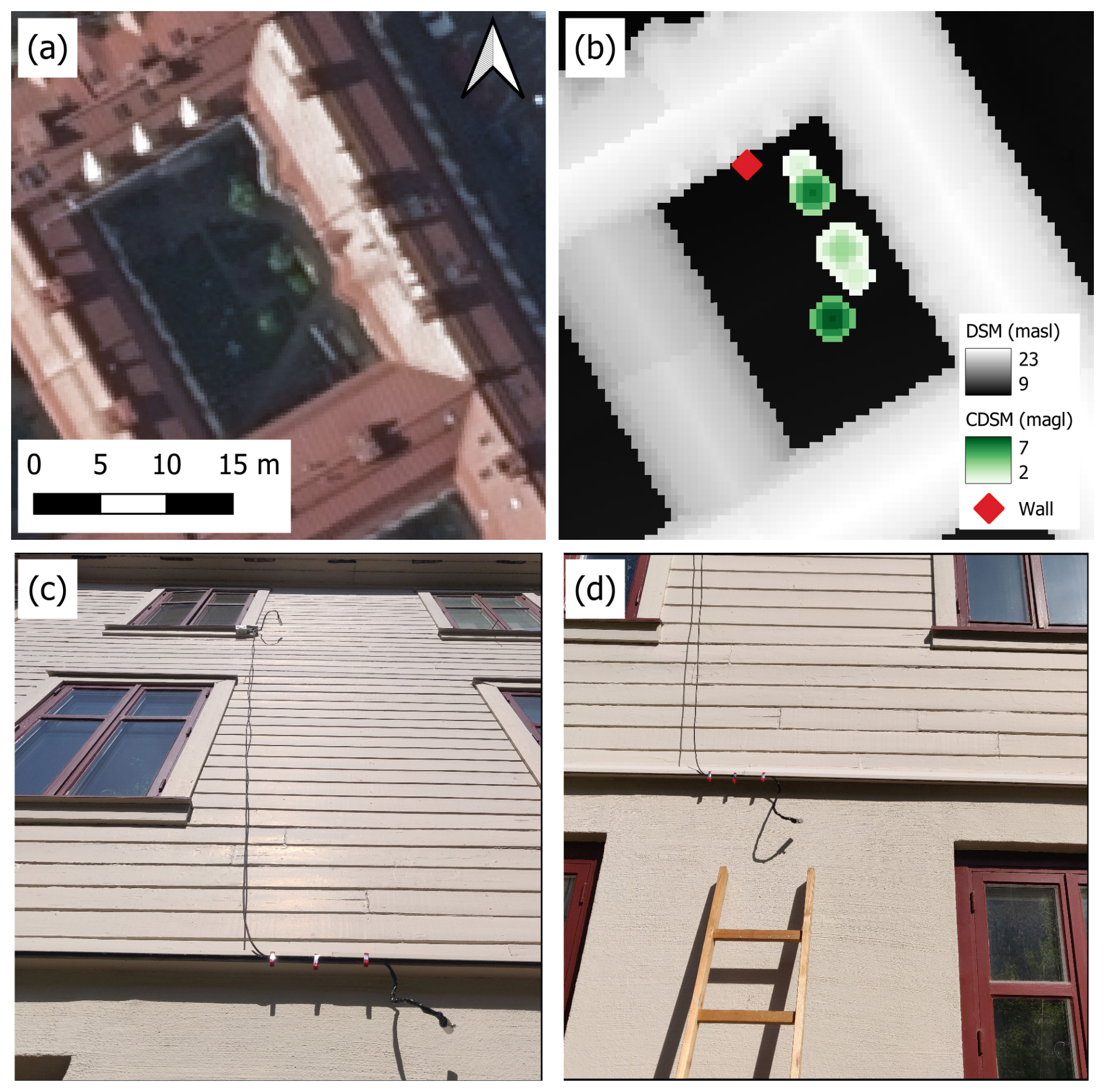
Figure 1 Orthophoto (© Lantmäteriet) (a) and digital surface model (DSM) and canopy digital surface model (CDSM) (b) of the courtyard surrounding the observed wall. The location of the wall is indicated by a red diamond. The observed walls with sensors can be seen in (c) and (d).

3 Results

Five days of simulated and observed wall T_s for the wooden and plaster brick walls are presented in Fig. 2a and b, respectively. These days are characterized by relatively high T_air, peaking at between 22–26 °C (Fig. 2c), and mainly clear weather conditions, with global shortwave radiation (K_↓) at solar noon peaking at 860–914 W m⁻² (Fig. 2c). Both walls show good agreement, with the simulated wall T_s consistently following the observed values. However, some deviations are evident, particularly around the time the wall becomes sunlit and in the nighttime. Around sunrise the simulated T_s for the wooden wall are underestimated at 2–6 °C (Fig. 2a). In the afternoon the simulated cooling rate of the wall is too slow, leading to overestimations of around 1–2 °C that continue into the nighttime. For the last two days, midday temperatures were underestimated by around 5 °C.

The simulated T_s for the plaster brick wall (Fig. 2b) overestimate up to 2 °C at midday during the first three days. Contrary to the wooden wall, the plaster brick wall underestimates from the evening into nighttime, with 1–3 °C, as an effect of a too rapid simulated cooling rate.

Figure 2 Plots showing five days of observed (solid) and simulated (dashed) wall surface temperature in 10 min temporal resolution for (a) the wooden wall and (b) the plaster brick wall. Grey areas show when the wall voxel is in simulated shade. Meteorological forcing data is given in (c), with direct solar radiation (K_dir) in solid, diffuse solar radiation (K_diff) in dashed and air temperature (T_air) in dotted lines.

Figure 3 shows the diurnal development for the whole study period (15 May–31 August 2023). The top panel (Fig. 3a) shows T_s for the wooden wall. The mean values of the simulation (dashed blue line) are aligned with the mean of the observations (solid line), with a small underestimation of 1–2 °C between 08:00–13:00. Before and after these hours, simulations are close to observations with a very small overestimation. The spread of the data can be explained by different weather conditions, ranging from fully overcast, shown as low daytime values, to high values correlating to clear weather conditions with high amounts of incoming solar radiation. Here, it is also noticeable that the simulations (in blue) diverge from the observations, with underestimations during intense solar radiation and overestimations in nighttime.

The plaster brick wall, presented in Fig. 3b, shows opposite patterns compared to the wooden wall. Here, simulations overestimate with 1 °C in daytime, and underestimates by 2–3 °C in nighttime. These patterns are also visible in the spread of the data, where simulations overestimate during intense solar radiation. There is a narrower spread for the plaster brick wall, compared to the wooden wall, which can be explained by their material characteristics, i.e. the wooden wall reacts much faster to changes in solar radiation.

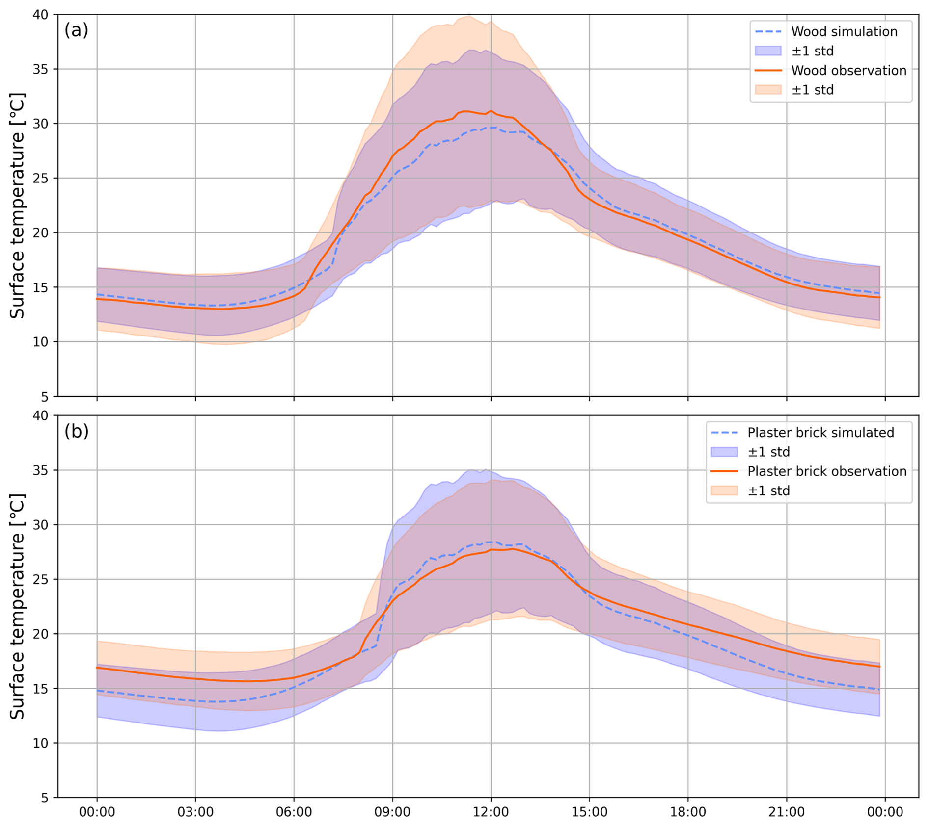
Figure 3 Plots showing wall surface temperatures from 15 May through to 31 August 2023 (107 d) for (a) the wooden wall and (b) the plaster brick wall. The dashed and solid lines show mean simulated and observed wall surface temperatures, respectively.

Scatter plots of 10 min simulated and observed T_s of the wooden wall, classified into five classes of mean K_↓ between 11:00–14:00 are presented in Fig. 4a–e, with all values given in Fig. 4f. For example, an entire day will be classified into $K_{\downarrow }<\mathrm{150}$ W m⁻² if the mean K_↓ between 11:00–14:00 on this day is below 150 W m⁻². The five classes are $K_{\downarrow }<\mathrm{150}$ W m⁻² (9 d), 150–300 W m⁻² (14 d), 300–450 W m⁻², (14 d), 450–600 W m⁻² (19 d) and $K_{\downarrow }>\mathrm{600}$ W m⁻² (51 d).

The first class ($K_{\downarrow }<\mathrm{150}$ W m⁻²) (Fig. 4a) shows high correlation between simulations and observations (R²=0.93) and low deviation of simulations (RMSE 0.82 °C). The three following classes (Fig. 4b–d) have lower correlations, partly because days in these classes are subject to partly cloudy weather, compared to the first class that is subject to overcast conditions. The last class (Fig. 4e) shows higher agreement between simulations and observations (R²=0.95). Overall, with 15 394 observation points (Fig. 4f), the simulations for the wooden wall correlate well with observed values (R²=0.93) and show relatively low RMSE (2.09 °C), indicating that the model performs well.

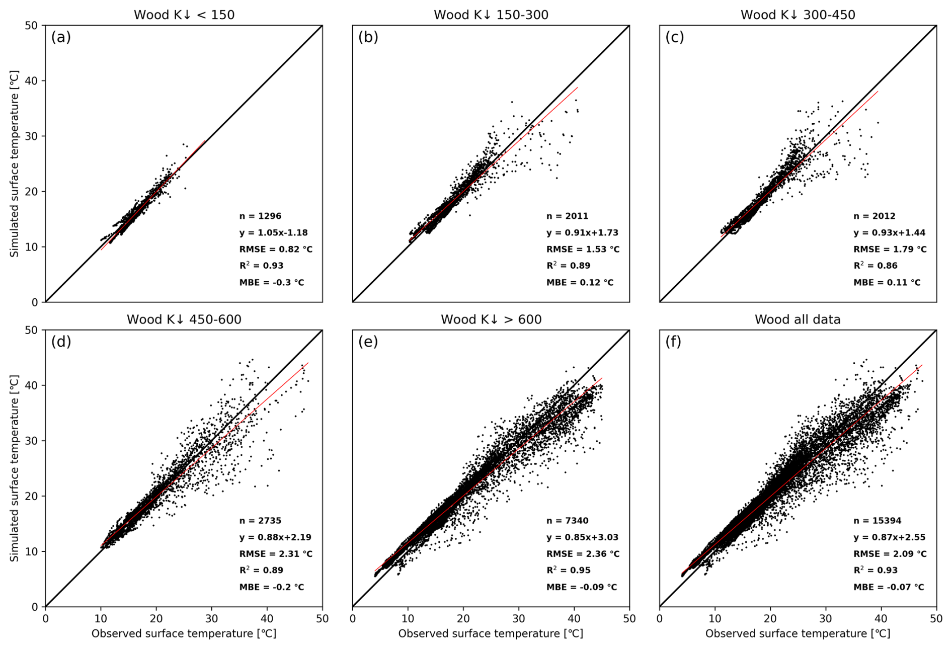
Figure 4 Scatter plots of 10 min simulated and observed T_s of the wooden wall, classified according to average incoming global shortwave radiation between 11:00–14:00 of (a) $K_{\downarrow }<\mathrm{150}$ W m⁻², (b) 150–300 W m⁻², (c) 300–450 W m⁻², (d) 450–600 W m⁻², (e) > 600 W m⁻², and (f) all data.

Similar scatter plots to those in Fig. 4, but for the plaster brick wall, are presented in Fig. 5. Correlations are generally good for all five classes. Best agreement can be seen in K_↓ > 600 W m⁻² (R²=0.95) (Fig. 5e), whereas lowest is evident in K_↓ < 150 W m⁻² (Fig. 5a) and K_↓ 300–450 W m⁻² (Fig. 5c) classes with R²=0.86. Highest deviation is found in K_↓ 450–600 W m⁻² (RMSE = 2.09 °C) (Fig. 5d), whereas lowest deviation is evident for K_↓ < 150 W m⁻² (RMSE = 1.46 °C) (Fig. 5a), which can be explained by low incoming shortwave radiation during overcast weather conditions, resulting in a T_s of the wall that is possibly close to T_air. All observations combined (Fig. 5f), simulated T_s show good agreement with observations (R²=0.94) and small deviations (RMSE = 1.94 °C).

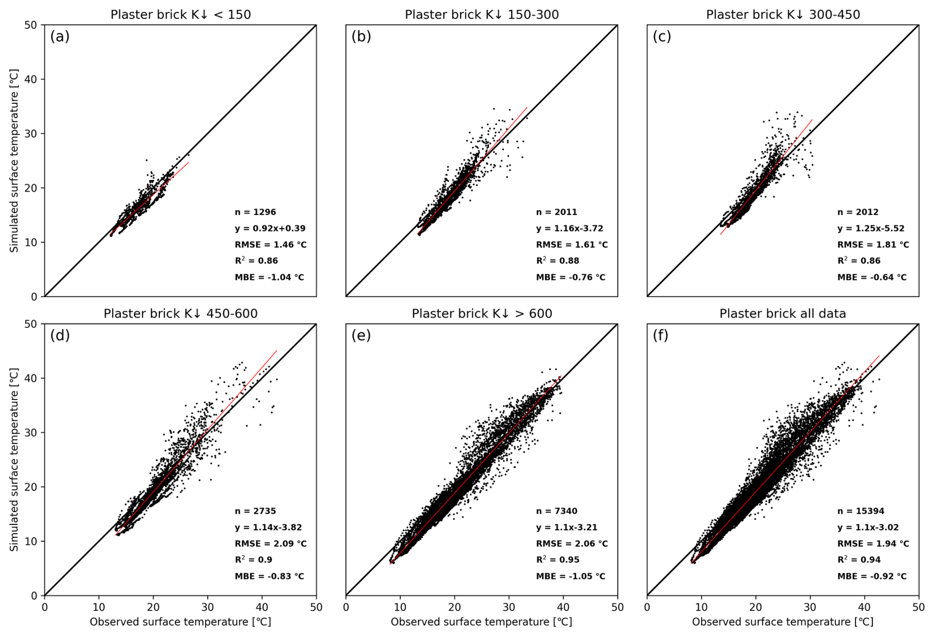
Figure 5 Scatter plots of 10 min simulated and observed T_s for the plaster brick wall, classified as for Fig. 4 into (a) $K_{\downarrow }<\mathrm{150}$ W m⁻², (b) 150–300 W m⁻², (c) 300–450 W m⁻², (d) 450–600 W m⁻², (e) > 600 W m⁻², and (f) all data.

Comparisons in T_mrt at different timesteps are presented in Fig. 6 to assess the effect of the new parameterization scheme for wall T_s with the previous method (Lindberg et al., 2008). The simulations are for 12 June 2023 (as shown in Fig. 2) and the different timesteps compared are (a) 00:00, (b) 03:00, (c) 06:00, (d) 09:00, (e) 12:00, (f) 15:00, (g) 18:00 and (h) 21:00.

The effect of the new scheme on nighttime T_mrt in the courtyard is small but noticeable, around 0.3 °C lower compared to the old version (v2022a) of SOLWEIG (Fig. 6a–b). At 06:00 in the morning (Fig. 6c), when the sun is above the horizon but still at a low elevation, more differences in T_mrt appear, with some areas having slightly higher values (0.4 °C), while others have slightly lower (−0.2 °C). At 09:00 (Fig. 6d), more pronounced differences appear, with areas close to the northwestern corner of the courtyard being up to 2.5 °C warmer compared to SOLWEIG v2022a. Here, the sun reaches most of the areas in this corner as the sun is in the east at around 35° elevation, meaning that the direct shortwave component is close to perpendicular to the walls, resulting in high amounts of radiation reaching these surfaces. This becomes evident when looking at the differences at 12:00 (Fig. 6e), when incoming shortwave radiation is higher but differences are smaller, as this is close to solar noon (∼ 55°) and therefore far from perpendicular to the wall. Nevertheless, differences are about 2.0 °C. At 15:00 when the sun is in the southwest, differences are up to 1.5–2.0 °C in the northeastern corner (Fig. 6f). Here, it is also evident that parts of the walls are shaded by the trees in this corner, which results in lower T_mrt ($\sim -\mathrm{1.5}$ °C). When the sun is in west (θ ≈ 270°) at 18:00, parts of the southeastern corner are sunlit. This results in ∼1.0 °C higher T_mrt with the new scheme, compared to the old one. In the last example (21:00), T_mrt is lower, $\sim -\mathrm{0.6}$ °C, compared with the old scheme. The sun is close to setting, at an elevation ∼5–6°. Thus, the courtyard and its walls are shaded.

Figure 6 Difference in mean radiant temperature (T_mrt) for SOLWEIG simulations with the new and old parameterizations for wall surface temperatures at (a) 12 June 2023 00:00, (b) 03:00, (c) 06:00, (d) 09:00, (e) 12:00, (f) 15:00, (g) 18:00 and (h) 21:00.

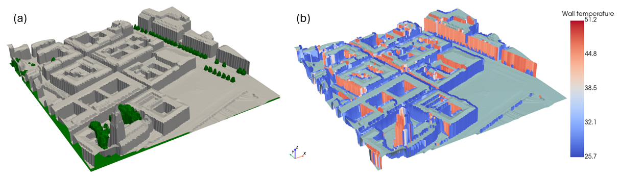
Figure 7 3D visualization of the (a) digital surface model (DSM) in grey and canopy digital surface model (CDSM) in green, in the area around Gustaf Adolfs Torg in central Gothenburg, and (b) simulated wall temperatures for the same area. The simulation is for 12 June 2023 17:00:00 UTC+1. Pixel and voxel size is 1 m. Produced with PyVista (Sullivan et al., 2019).

Since the new wall temperature scheme presented here enables calculation of the variation in T_s at different heights, visualization in 3D provides important information on the distribution of T_s throughout the model domain. As an example, Fig. 7 presents a 3D visualization of the surface model used in SOLWEIG (Fig. 7a) and wall T_s in central Gothenburg on 12 June 2023 17:00 UTC+1 (Fig. 7b). The shadow-casting algorithm in SOLWEIG captures shadows from trees, which are visible along the wall in the top right of the figure. In this area, lower wall temperatures (blue) in shade can be observed, contrasting with the sunlit parts of the wall.

To analyze the effect of the input variables of the model on the resulting T_s, a sensitivity test was conducted. The test is based on an unobstructed wall facing south forced with meteorological data from 13 June 2023 (see Fig. 2c). Default values are given in Table 2. Default albedo and emissivity were 0.5 and 0.95, respectively.

Table 2 Default values of thermal conductivity (λ), density (ρ) and specific heat capacity (C) for the dummy wall used in the sensitivity test.

As mentioned in the methods, specific heat capacity and density has no effect on the resulting T_s as any changes in these two variables are cancelled out by corresponding changes in t. The remaining input variables, emissivity, albedo, thermal conductivity and wall thickness, influence T_s to different extents. The three first variables are depicted in Fig. 8. The influence of wall emissivity is relatively small (Fig. 8a), and T_s increases with a decrease in emissivity, as expected. There is less radiative cooling and therefore T_s increases. Albedo (Fig. 8b), on the other hand, influences the amount of absorbed shortwave radiation. As such, T_s increases with a decrease in albedo as more shortwave radiation is absorbed by the wall. A decrease in thermal conductivity (Fig. 8c), likewise, leads to an increase in T_s. Lower thermal conductivity means that less heat is conducted through the material and instead is used to heat up the surface.

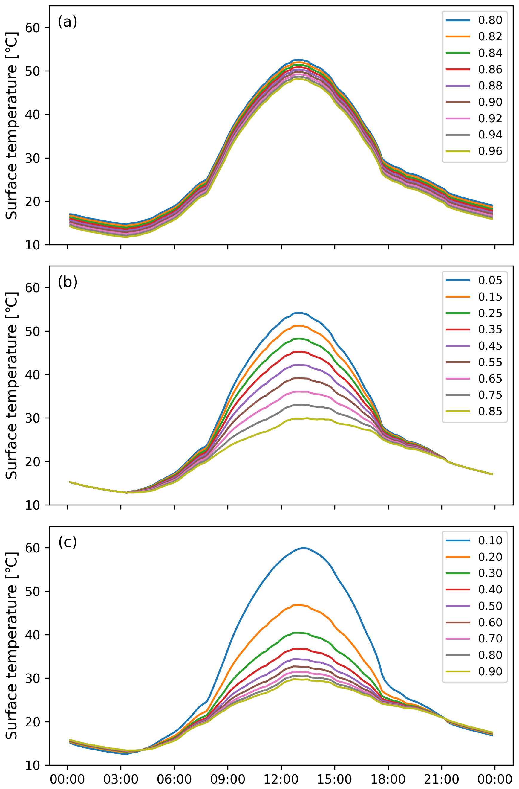
Figure 8 Simulated wall surface temperatures for an unobstructed wooden wall facing south with different (a) emissivity, (b) albedo and (c) thermal conductivity (W m⁻¹ K⁻¹).

The influence of wall thickness on T_s differs from the previous variables as it also depends on the other thermal properties of the material. Three examples are shown in Fig. 9: wood (Fig. 9a), brick (Fig. 9b) and concrete (Fig. 9c). The wooden wall is very sensitive to changes in wall thickness. As evident in Fig. 9a, T_s deteriorates already between 0.04 and 0.06 m. For the brick wall, in Fig. 9b, T_s starts to deteriorate after 0.2 m, indicating that it is less sensitive to changes in thickness. In the last example (Fig. 9c) the concrete wall starts to deteriorate after 0.5 m.

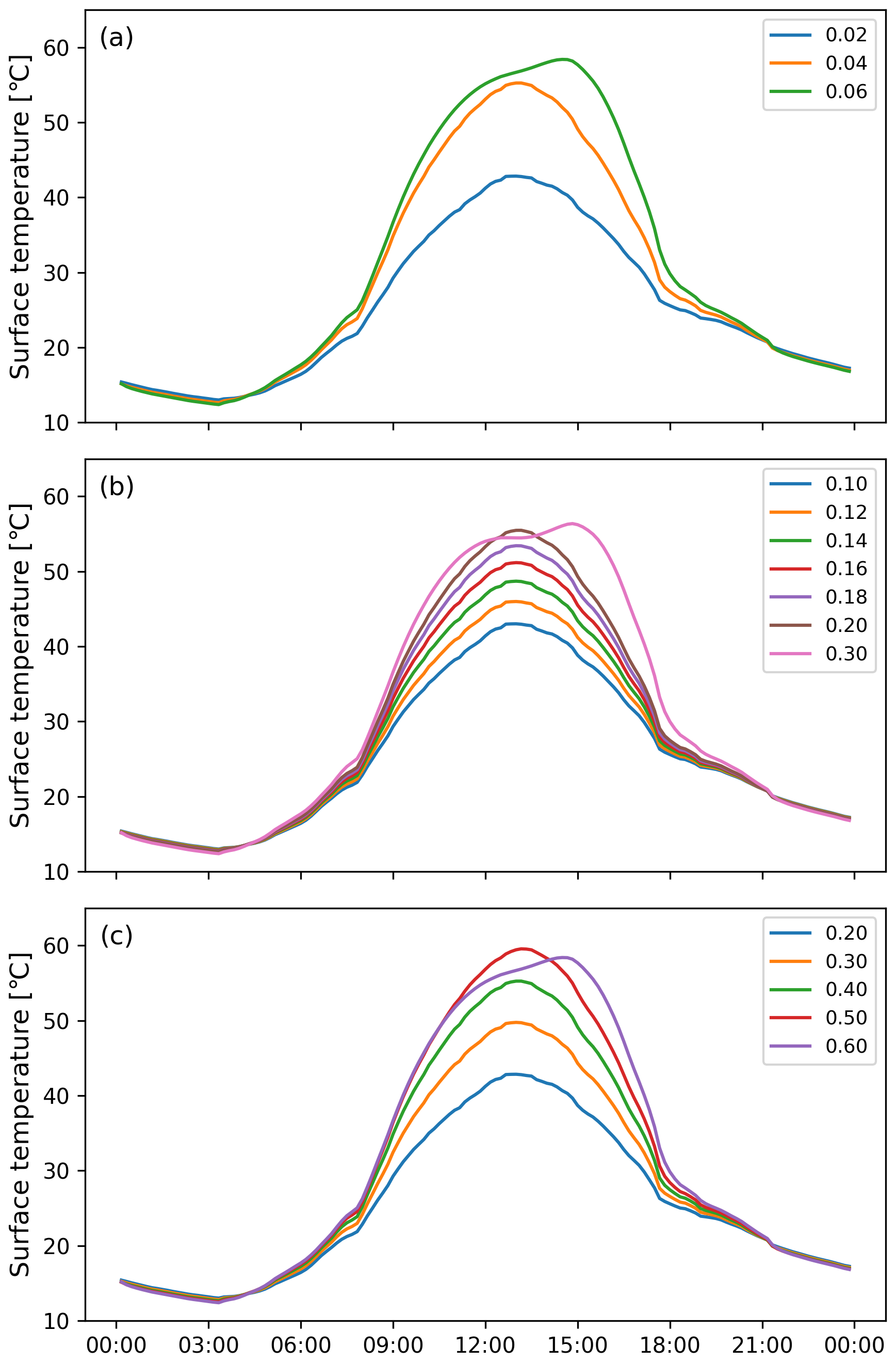
Figure 9 Simulated wall surface temperatures for an unobstructed wall facing south with different wall thickness (m) for three different materials: (a) wood, (b) brick and (c) concrete.

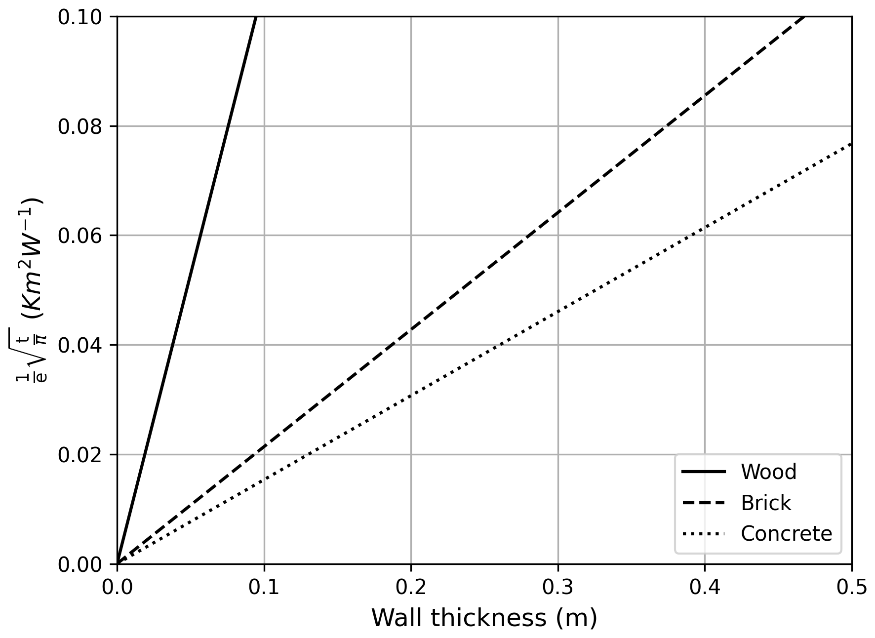
The previous figure (Fig. 9) indicates that T_s starts to deteriorate at different wall thickness depending on material. For example, T_s for wood starts to deteriorate at wall thickness < 0.06 m, brick < 0.3 m and concrete at 0.5–0.6 m. The ratio $R=\frac{\mathrm{1}}{e}\sqrt{\frac{t}{\mathit{\pi }}}$ (K m² W⁻¹) against wall thickness is visualized in Fig. 10. Here it is visible that these wall thicknesses correspond to R≈0.06 K m² W⁻¹ for wood and brick. Concrete, that is a substantially more inert material, potentially has a higher threshold for its R, but is nevertheless close to 0.06. The ratio R is a good indicator for when the model might start to behave erratically and can be used to warn potential users of too thick walls. Because we are using a characteristic time t with our semi-infinite step heating approach, the estimated R reduces to a simple function of wall thickness over thermal conductivity, $R=\frac{L}{\mathit{\pi }\sqrt{\mathit{\pi }}\mathit{\lambda }}$, that can be used to estimate the maximum wall thickness $L_{\max }=\mathit{\pi }\sqrt{\mathit{\pi }}\mathit{\lambda }R$. Using a conservative R=0.05 K m² W⁻¹ instead of 0.06 K m² W⁻¹ gives L_max=0.047, 0.234 and 0.326 m for wood, brick and concrete, respectively.

Figure 10 Relationship between $\frac{\mathrm{1}}{e}\sqrt{\frac{t}{\mathit{\pi }}}$ (K m² W⁻¹) and wall thickness (m).

4 Discussion

A new and simple method for simulations of wall T_s has been presented. This new parameterization scheme, based on the works of Boue and Fournier (2009), enables estimations of wall T_s for individual vertical pixels described as voxels. This can be compared to the previous method where wall T_s was estimated for either sunlit or shaded façades (Lindberg et al., 2008).

The five-day examples presented in Fig. 2 showcase that simulations follow observations. High agreement between simulations and observations is also evident from the statistics in Figs. 4 and 5, even though correlations decrease with cloudiness, i.e. neither overcast nor clear weather conditions. The lower correlations under cloudy conditions can easily be explained by the fact that the SOLWEIG model does not solve for explicit cloud cover but depends on observations of shortwave radiation, and that observations originate from a weather station located approximately 2.3 km from the wall of interest for the model evaluation. Nevertheless, R² values are high (0.93 and 0.94 for wood and plaster brick respectively), and based on 15 394 observation points, covering the entire summer of 2023. RMSE are also low (2.09 and 1.94 °C). These can be compared to RMSE values for simulated T_s of walls on traditional (3.3 °C) and contemporary (7.4 °C) buildings in Dejvice, Prague, Czech Republic, with the PALM-4U model (Resler et al., 2021) and the T_s simulated with the ENVI-met model for a brick wall covered with plaster (R²=0.98–0.99, RMSE = 1.03–1.25) (Simon, 2016). The better performance of the ENVI-met simulations compared to our method could potentially be explained by the fact that (i) ENVI-met make use of a 7-node conduction model and (ii) their observations are for a controlled building test site, whereas our results are from a real-world example, where we have less knowledge of the thermal properties of the walls. Other examples of models where our results compare are e.g. TUF3D (Krayenhoff and Voogt, 2007) and SOLENE (Hénon et al., 2012). The temperature range for the wooden wall is larger than that of the plaster brick wall, which could be explained by the material characteristics. The wooden wall has a lower thermal effusivity compared to the plaster brick wall, meaning that the wooden wall is more sensitive to changes in radiation. Thus, the T_s of the wooden wall will fluctuate more, especially during cloudy conditions. The lower thermal effusivity also explains why the T_s of the wooden wall is higher compared to the plaster brick wall.

The present simulation of wall T_s may look simple since there are only two variables involved (T_air and net radiation of the wall). However, there are several steps to get the net radiation of the wall. The shortwave radiation depends on the angle between the direct solar radiation and the wall but also reflected radiation from the surrounding surfaces and shadow patterns. The estimation of the outgoing longwave radiation is problematic since it requires information on T_s of the wall, i.e. the same variable we aim to simulate. As a proxy we use an iterative process starting with the T_s from the previous timestep. Already after the first iteration the wall T_s is stabilized within a few tenths of a degree, which we consider to be close enough to calculate the outgoing longwave radiation.

The wall surface energy balance is of course not only influenced by the net radiation but also by the sensible heat flux to/from the air and the heat flow within the wall. Both these processes are forced by the wall T_s as well as other atmospheric conditions (e.g. wind/turbulence). However, the close connection between the observed and simulated T_s in our study shows that net radiation dominates heating and cooling of the wall surfaces. A similar conclusion was made by Resler et al. (2021). They found it striking that the agreement was better between observed and modelled wall T_s during summer episodes with strong radiative forcing. However, the observed wall T_s of plastered brick walls both in our study and in the study by Resler et al. (2021) were higher than the simulated after the daytime maximum, which indicates an influence of heat stored in the wall earlier during the day. Higher observed than simulated minimum wall T_s, as also noted by Resler et al. (2021), point to an addition of stored heat to the wall surface. On the other hand, the thinner wooden wall with less ability to store heat was cooler than the simulation during the night.

The new parameterization scheme has enabled better estimations of wall T_s and introduced estimations of shading on walls from surrounding buildings and trees (e.g. Fig. 7b). This results in differences in T_mrt between this new version and previous versions of SOLWEIG. Some of these differences are presented in Fig. 6 and show that the location of the sun has an effect on T_mrt. This is explained by the estimation of wall T_s for individual voxels, where each voxel has its own relation to the location of the sun because of its material characteristics (thermal effusivity, albedo, emissivity) but not the least aspect. The aspect of the wall, i.e. its orientation, influences how much of the direct shortwave radiation that it is exposed to. Previous studies have concluded that the old parameterization in SOLWEIG led to deviations in simulated wall T_s that affected T_mrt (Gál and Kántor, 2020; Wallenberg et al., 2023a).

Gál and Kántor (2020), using SOLWEIG, saw deviations in simulated T_mrt in proximity to wall surfaces and suggested a separate surface temperature parameterization scheme. Some of the overestimations were potentially reduced by around 3 °C with the introduction of patches for short- and longwave radiation described in Wallenberg et al. (2020, 2023a). The new parameterization scheme for wall T_s should improve these deviations further. For example, underestimations were seen in vicinity of sunlit areas (Gál and Kántor, 2020). Here, we show (e.g. Fig. 6d) that the new wall surface scheme calculates higher T_mrt close to sunlit walls (up to 2.5 °C for our case). A small decrease is also noticeable under the trees (Fig. 6f–g). These differences come from the directionality of the walls and accounting for whether they are sunlit or shaded, which was previously not possible.

Kim and Ham (2024) found deviations in simulated T_s of asphalt, plywood and soil, and suggested improvements in thermophysical attributes of construction materials in calculations in SOLWEIG. Although their study referred to horizontal surfaces (e.g. ground and roofs) the suggestions are in line with what has been presented in this paper. The old parameterization scheme for wall T_s is based on the parameterization scheme for ground surface temperatures utilized in SOLWEIG. This scheme was initially developed by Bogren et al. (2000) and refined by Lindberg et al. (2016) and is based on a sinusoidal curve that peaks at a set time. For ground surfaces, this peak in time might be accurate as it occurs not long after solar noon. For walls, however, one peak time for the entire model domain will lead to differences in T_s, depending on the aspect of the wall. Peak time of a wall facing east will for example occur in the morning, whereas it will occur in the afternoon or evening for a wall facing west. The T_s scheme presented here, thus, is an improvement in SOLWEIG, but for wall surfaces. The method presented could, however, be useful for ground surfaces as well.

Even though the model performs well, there are some shortcomings. For example, the spatial input data is pixel based. This leads to deviations when estimating wall aspects which could be seen in Fig. 7b (stripe effect). Although the accuracy of aspect calculations is high in mid-sections of the walls, deviations occur close to corners. Other potential sources of error could be the material characteristics used here, i.e. thermal conductivity, wall thickness, emissivity and albedo. In addition to this, there is a possibility that there are deviations based on longwave radiation reflected from the background, i.e. the opposite of our sensors (Apogee Instruments, 2024b), something that is difficult to estimate in urban areas with many different surfaces that have different emissivity. In relation to the sensors, there is also a possibility that there are micro-shadows on e.g. the wooden wall from the microscale spacing between the boards. Other shortcomings that are likely to influence our results are that we are modeling environmental radiative forcings at the surface of the wall, i.e. input short- and longwave radiation. As they are simulated, they are not perfect, with impacts on the resulting T_s. This also goes for the properties of the wall surfaces, e.g. albedo, emissivity, thermal conductivity and wall thickness. Similar conclusions are described in Johnson et al. (1991), where their simulated rural and urban surface temperatures performed better when the specification of input thermal properties and environmental forcings were most complete and accurate. Similar conclusions can be given about the basis of our step heating approach in Boue and Fournier (2009), where they have complete control over the forcing (heat pulse), thermal properties and not the least environmental conditions of their lab setting.

It is evident from the sensitivity analysis that there are constraints in the model. For example, there are limits to how thick a wall can be, depending on its thermal conductivity (Fig. 9). The presented solution, using R to estimate L_max to get an indication on when the model might become unstable can hopefully guide users (e.g. Fig. 10). In addition to this, the sensitivity analysis shows that albedo and thermal conductivity have largest effects on T_s and emissivity least (Fig. 8). These results are expected. An increase in albedo should lead to a decrease in T_s as less shortwave radiation is absorbed. An increase in thermal conductivity leads to more energy propagating through the material and less energy at its surface, i.e. lower T_s. A material with higher emissivity has higher radiant cooling and therefore a lower T_s. Thermal conductivity and emissivity are material properties that should affect the thermal comfort of a human, i.e. if they are changed, so is the exposure to a human. A change in albedo, on the other hand, leads to less absorption of heat by a surface (if it is increased), i.e. decrease in longwave radiation, and increases the reflectivity of shortwave radiation. Thus, a human would be exposed to less longwave radiation but more shortwave radiation (Erell et al., 2014).

The new scheme has only introduced four new input parameters to the SOLWEIG model: thermal conductivity, density, specific heat capacity and thickness of the wall. These parameters are easily accessible in literature (e.g. CIBSE, 2015). Three materials are available in the new publicly available SOLWEIG model: brick, concrete and wood. Other materials can simply be added to the parameter file in SOLWEIG. One drawback with the new scheme is the computational complexity. Running the model for one day at 10 min resolution (144 time steps) took approximately 5 min with the newly implemented wall scheme parameterization, compared to around 1 min without it, on an Intel i7-7700 CPU @ 3.6 GHz with 16 GB RAM. However, this is still faster than most other models designed for similar purposes.

Future efforts will include improvements of the ground surface calculations. Initial results indicate that the force-restore method is a well-suited framework for this application. Moreover, the parameterization scheme should be evaluated for other wall surfaces and urban environments, as well as a deeper evaluation of the behavior of walls and their influence on the microclimate and thermal comfort of humans.

5 Conclusions

We have presented a new parameterization scheme for calculations of wall T_s. The scheme is simple and fast, with only four new input parameters: thermal conductivity, density, specific heat capacity and wall thickness, together with a heat flux density, in this case the heat balance of the wall surface. The performance of the scheme is high for the two assessed wall surfaces, wood (R²=0.93, RMSE = 2.09 °C) and plaster brick (R²=0.94, RMSE = 1.94 °C), making it comparable to heat conductivity models utilized in other models for microclimate.

The implementation of the scheme in the SOLWEIG model has enabled more realistic estimations of wall T_s by incorporating wall aspects and material characteristics. In the examples presented here this has led to differences in T_mrt of up to 2.5 °C compared to the previous version of SOLWEIG.

With this new scheme SOLWEIG can now be used to understand how different building materials influence outdoor thermal comfort. The high accuracy indicated by our results combined with the computational speed suggests that this approach can be used in other areas where T_s of walls are important, for example building energy and urban energy balance models.

The new version of SOLWEIG presented here and its associated datasets are available in Wallenberg et al. (2025a, b).