Runoff evaluation in an Earth System Land Model for permafrost regions in Alaska

Modeling of hydrological runoff is essential for accurately capturing spatiotemporal feedbacks within the land–atmosphere system, particularly in sensitive regions such as permafrost landscapes. However, substantial uncertainties persist in the terrestrial runoff parameterization schemes used in Earth system and land surface models. This is particularly true in permafrost regions, where landscape heterogeneity is high and reliable observational data are scarce. In this study, we evaluate the performance of runoff parameterization schemes in the Energy Exascale Earth System Model (E3SM) land model (ELM). Our proposed framework leverages simulation results from the Advanced Terrestrial Simulator (ATS), which is a physics-based integrated surface/subsurface hydrologic model that has been successfully evaluated previously in Arctic tundra regions. We used ATS to simulate runoff from 22 representative hillslopes in the Sagavanirktok River basin, located on the North Slope of Alaska, then compared the output with ELM's parameterized representation of total runoff. Results show that (1) ELM's total runoff was the same order of magnitude as the ATS simulations, and both models were similarly variable over time; (2) minor adjustments to coefficients in ELM's runoff parameterization improved the match between the ATS simulation and ELM's parameterized representation of annual and seasonal total runoff; (3) overall, runoff responses in ATS and ELM are more similar in flat hillslope environments compared to steep hillslopes; and (4) shallower active layer thicknesses and higher precipitation simulations resulted in lower correlations between the two models due to greater total runoff. By incorporating the optimized runoff coefficients from the Sagavanirktok River basin into ELM, the simulated total runoff better matched the streamflow observations at a small watershed located on the Seward Peninsula of Alaska. Our findings revealed important insights into the effectiveness of runoff parameterizations in land surface models and pathways for improving runoff coefficients in typical Arctic regions.

1 Introduction

Runoff parameterization schemes play a critical role in the accuracy of Earth system models, particularly in sensitive environments such as high latitude permafrost regions. These areas are increasingly vulnerable to climate variability, and the hydrological responses associated with warming temperatures can have profound implications for ecosystems and water resources (Bring et al., 2016; Yang and Kane, 2020). The interplay between hydrology and climate dynamics in permafrost zones is complex because conditions such as vegetation, snow, soil wetness, ground ice content, and biogeochemical activities vary significantly over small spatial extents (Holmes et al., 2013; Bennett et al., 2022). At the same time, Earth system models and land surface models are designed for pan-Arctic scale simulations, creating a strong mismatch between the scale at which these processes occur and the models designed to represent them (Lique et al., 2016).

Despite the importance of runoff in accurately modeling ecosystem dynamics, considerable uncertainties remain in the parameterization schemes employed by land surface models. The accuracy of one process often depends on the scheme chosen for another, creating interdependencies that can complicate model accuracy. In permafrost regions, the presence of ice-rich permafrost can disrupt water infiltration processes, leading to increased surface runoff and altered drainage patterns (Kuchment et al., 2000; Walvoord and Kurylyk, 2016; Bennett et al., 2023). These heterogeneous conditions complicate efforts to accurately represent hydrological dynamics and highlight the necessity for improved modeling techniques. The scarcity of observational data and unmeasurable model parameters exacerbate these challenges, resulting in significant discrepancies between model outputs and real-world hydrological behavior (Bring et al., 2016; Clark et al., 2015, 2017). Addressing these uncertainties is essential for developing reliable predictive models that can support resource management and conservation efforts within rapidly changing Arctic ecosystems (Schädel et al., 2024).

Recent land model intercomparison projects (e.g., Boone et al., 2004; Lawrence et al., 2016; Collier et al., 2018; Mwanthi et al., 2024) have summarized various implementations of runoff schemes, ranging from simple bucket models to more advanced topography-based runoff models. These studies highlight significant variability in lateral surface runoff and subsurface runoff (baseflow) among different land models. Clark et al. (2015) emphasized the need to integrate groundwater-surface water interactions in Earth system models, while Maxwell et al. (2014) demonstrated the benefits of coupling surface and subsurface models for better predictions in complex landscapes. By improving soil freeze-thaw processes and incorporating soil heterogeneity, Liang and Xie (2001) and Swenson et al. (2012) achieved better runoff alignment with observed streamflow. Fan et al. (2019) identified lateral water flow as a crucial runoff component for the water cycle in the Arctic, with additional studies highlighting significant uncertainties in runoff parameterization schemes in high-latitude cold regions (e.g., Zheng et al., 2017; Hou et al., 2023; Abdelhamed et al., 2024). These efforts collectively highlight the pressing need to refine hydrological runoff simulations to improve predictions, particularly in permafrost regions as climate change intensifies.

Many previous studies have evaluated runoff parameterization by comparing different schemes against streamflow observations at large scales and coarse resolutions (e.g., Niu et al., 2007; Li et al., 2011; Swenson et al., 2012; Zheng et al., 2017; Li et al., 2024), however, high-quality streamflow data that can be used to validate runoff production are difficult to obtain in permafrost regions. This highlights the need for a more cost-effective and flexible framework to rapidly evaluate parameterization effectiveness using alternative approaches, for example, leveraging simulations from robust computational tools for physics-based permafrost thermal hydrology processes. The permafrost thermal hydrology capability (Painter et al., 2016) in the Advanced Terrestrial Simulator (ATS) (Coon et al., 2020) has emerged as a valuable tool in this regard. ATS has been successfully compared to snow depth, supra-permafrost water table depth, and vertical profiles of soil temperatures (Atchley et al., 2015; Harp et al., 2016; Jan et al., 2020) and to catchment-scale evapotranspiration and runoff (Painter et al, 2023) in continuous permafrost regions. ATS's permafrost thermal hydrology capabilities have been used in a variety of modeling studies (e.g., Atchley et al., 2015; Sjöberg et al., 2016; Jafarov et al., 2018; Abolt et al., 2020; Jan and Painter, 2020; Hamm and Frampton, 2021; Painter et al., 2023)

This study aims to evaluate and improve the parameterization of runoff processes in the Department of Energy's Energy Exascale Earth System Model (E3SM) Land Model (ELM) (e.g., Oleson et al., 2013; Bisht et al., 2018; Xu et al., 2022; Shi et al., 2024) using detailed simulations from ATS. We quantitatively assess ELM's runoff parameterization, focusing on total runoff rather than individual components separately. The method we detail in this work directly addresses the scale gap between local- to global-scale process representation in models, using intercomparison with local-scale ATS simulations and parameters updates in ELM to improve Arctic runoff processes. By adopting a total water mass balance perspective, this approach provides insights into the strengths and limitations of ELM's runoff schemes, ultimately enhancing its predictive capabilities in Arctic environments. Additionally, it offers a comprehensive understanding of how landscape features and thermal hydrological processes interact in permafrost regions.

2 Model description

2.1 ELM runoff parameterization schemes

The runoff parameterization within ELM is designed to represent how water moves across the land surface between grid cells and is influenced by numerous factors, including soil moisture, topography, vegetation cover, etc. ELM's runoff scheme (ported from CLM v4.5, Oleson et al., 2013) is based on a simple TOPMODEL-based concept with a simplified topography representation (Niu et al., 2005). The runoff in ELM is partitioned into surface and subsurface flows, both of which are assumed to be related to water storage, vertical infiltration, and groundwater-soil water interactions (Beven and Kirkby, 1979; Niu et al., 2005, 2007). There are more than twenty runoff components (variables) defined in ELM, but essentially, they can be categorized into three groups in a simulation with fixed land use: (i) surface runoff, (ii) subsurface runoff, and (iii) runoff from overland water bodies like wetlands, lakes, and glaciers. The top 10 layers in ELM considered soil to a depth of ∼ 3.8 m and are hydrologically and biogeochemical active. The remaining five ground layers in each column are considered to be dry bedrock that extend to a depth of ∼ 42.1 m. The discretization of the fifteen layers, including their depths and thicknesses, is described in Sect. S1 and Table S1 in the Supplement. Here, we only explicitly list the key equations representing the crucial components of the former two groups representing for surface/subsurface runoff; for a more detailed description of the underlying physics and complete formulations, readers are referred to existing literature (Oleson et al., 2013; Niu et al., 2005; Bisht et al., 2018; Liao et al., 2025).

Surface runoff is composed of two components: (i) outflow from the saturated portion of a grid cell with excess water, q_over , and (ii) outflow from surface water storage such as a pond, q_h2osfc. The first term is written as:

$$\begin{array}{}\text{(1)}& q_{\mathrm{over}}=q_{\mathrm{liq},\mathrm{0}}{f}_{\max }\exp \left(-\mathrm{0.5}{f}_{\mathrm{over}}{Z}_{\mathrm{\nabla },\mathrm{perch}}\right)\end{array}$$

where q_liq,0 is the sum of liquid precipitation reaching the ground and melt water from snow (kg  m⁻² s⁻¹); f_max is the ratio of the area that has higher compound topographic index (CTI) values than the mean CTI value of the grid cell, with a consideration of geomorphological features; f_over is a decay factor that is often calibrated using the recession curve of the observed hydrograph, taken as 0.5 m⁻¹; Z_∇,perch is the perched groundwater table depth (m) within the thawed soil layers. The second term is formulated as:

$$\begin{array}{}\text{(2)}& q_{\mathrm{h}\mathrm{2}\mathrm{osfc}}=k_{\mathrm{h}\mathrm{2}\mathrm{osfc}}{f}_{\mathrm{connected}}\left(W_{\mathrm{sfc}}-W_{\mathrm{c}}\right){\displaystyle \frac{\mathrm{1}}{\mathrm{\Delta }t}}\end{array}$$

where the storage coefficient k_h2osfc=sin(β) is a function of grid cell mean topographic slope β (in radians); f_connected is the fraction of the inundated portion of the interconnected grid cell, calculated as $f_{\mathrm{connected}}={\left(f_{\mathrm{h}\mathrm{2}\mathrm{osfc}}-\mathrm{0.5}\right)}^{\mathrm{0.14}}$, which is equal to 0 if f_h2osfc is smaller than 0.5, and the f_h2osfc is the fraction of the area that is inundated. W_sfc represents surface storage water (kg m⁻²), determined by the surface-inundated fraction f_h2osfc, the slope β, the ponded water height, and microtopographic features. W_c is the amount of surface water present when f_h2osfc=0.5; and Δt is the model time step (0.5 h was used in this study).

Subsurface runoff is also composed of two components: (i) drainage in the frozen soils where the groundwater table remained dynamic under partially frozen conditions, q_drain, and (ii) drainage from the thawed active layer, q_drain,perch. The first term is based on the following exponential relationship:

$$\begin{array}{}\text{(3)}& q_{\mathrm{drain}}={\mathrm{10}}^{{\mathrm{\Theta }}_{\mathrm{ice}}}\cdot \mathrm{10}\sin \left(\mathit{\beta }\right)\cdot \exp \left(-\mathrm{2.5}{Z}_{\mathrm{\nabla }}\right)\end{array}$$

where Θ_ice is an exponent of the ice impedance factor. It is calculated as ${\mathrm{\Theta }}_{\mathrm{ice}}=-\mathrm{6}\left({\sum }_{i=jwt}^{N_{\mathrm{levsoi}}}{S}_{\mathrm{ice},i}\mathrm{\Delta }{Z}_{\mathrm{i}}/{\sum }_{i=jwt}^{N_{\mathrm{levsoi}}}\mathrm{\Delta }{Z}_{\mathrm{i}}\right)$, where S_ice,i is the saturation degree of ice in soil layer i; ΔZ_i is the layer thickness; jwt is the index of the layer directly above the water table; and N_levsoi=15 refers to the total number of soil layers. Z_∇ is the groundwater table depth (m). It should be noted that for continuous permafrost or frozen soil, its drainage is equal to zero or tiny values, and here the last term in Eq. (3) is reduced to a very small value, i.e., 2.8 × 10⁻¹⁰. The second term refers to the lateral drainage from the perched saturated zone between layers N_perch and N_frost, written as:

$$\begin{array}{}\text{(4)}& \begin{array}{rl}{q}_{\mathrm{drain},\mathrm{perch}}& ={\mathrm{10}}^{-\mathrm{5}}\sin \left(\mathit{\beta }\right)\\ & \left[{\sum }_{i=N_{\mathrm{perch}}}^{i=N_{\mathrm{frost}}}{\mathrm{10}}^{-\mathrm{6}\left(\frac{S_{\mathrm{ice},i}+S_{\mathrm{ice},\mathrm{i}+\mathrm{1}}}{\mathrm{2}}\right)}{k}_{\mathrm{sat},i}\mathrm{\Delta }{Z}_{\mathrm{i}}\right]\\ & \left(Z_{\mathrm{frost}}-Z_{\mathrm{\nabla },\mathrm{perch}}\right)\end{array}\end{array}$$

where k_sat,i is soil hydraulic conductivity (m s⁻¹) at saturated unfrozen status in soil layer i. Z_frost is the frost table defined as the shallowest frozen layers having an unfrozen layer above it (m). Z_∇,perch is the perched groundwater table depth (m) within the thawed layers above icy permafrost ground.

In this study, the total runoff from ELM is calculated as the sum of the above four runoff components, expressed as $q_{\mathrm{total}}=q_{\mathrm{drain}}+q_{\mathrm{drain},\mathrm{perch}}+q_{\mathrm{over}}+q_{\mathrm{h}\mathrm{2}\mathrm{osfc}}$ (with units in mass water flux, kg m⁻² s⁻¹).

2.2 ATS runoff generation schemes

ATS solves integrated surface/subsurface flow in complex topographic landscapes with complex soil structures, which can capture a wide array of processes and their interactions to produce a holistic system understanding of a system (Painter et al., 2016; Coon et al., 2020; Gao and Coon, 2022). As a physics-based hydrological model, ATS uses physically based representations for surface runoff, subsurface runoff, and river routing. Here, only the key governing equations are presented.

The subsurface variably saturated flow is based on the Richards equation with phase change to solve the conservation of water mass, written as:

$$\begin{array}{}\text{(5)}& {\displaystyle \frac{\partial }{\partial t}}\left[\mathrm{\varnothing }\left({\mathit{\omega }}_{\mathrm{g}}{m}_{\mathrm{g}}{s}_{\mathrm{g}}+m_{\mathrm{l}}{s}_{\mathrm{l}}+m_{\mathrm{i}}{s}_{\mathrm{i}}\right)\right]=-\mathrm{\nabla }\cdot \left(m_{\mathrm{l}}{\mathit{q}}_{\mathrm{l}}\right)+Q_{\mathrm{w}}\end{array}$$

where ∅ is porosity; the subscripts g, l, and i refer to the gas, liquid, and ice phases; ω is the gaseous mole fraction (mol mol⁻¹) referring to a molar fraction of water vapor within all gas in the pore space; m is the molar density of a particular phase (mol m⁻³); s is saturation ($s_{\mathrm{g}}+s_{\mathrm{l}}+s_{\mathrm{i}}=\mathrm{1})$; and Q_w refers to sources and sinks (mol s⁻¹). The Darcy velocity (m s⁻¹) is presented as ${\mathit{q}}_{\mathrm{l}}=-k_{\mathrm{int}}{k}_{\mathrm{rl}}/{\mathit{\mu }}_{\mathrm{l}}\left(\mathrm{\nabla }{P}_{\mathrm{l}}+{\mathit{\rho }}_{\mathrm{l}}\mathit{g}\mathrm{\nabla }z\right)$ , where k_int is intrinsic permeability (m²), k_rl is relative permeability, μ_l is dynamic viscosity (Pa s), P_l is pressure head (Pa), ρ_l is water density (kg m⁻³), g is the gravitational acceleration (m s⁻²), and z is the vertical elevation (m). The vapor pressure in the pore space is assumed to be in equilibrium with the liquid phase above the freezing temperature and in equilibrium with the ice phase below freezing. The parameterizations and constitutive relationships, such as the van Genuchten soil water retention curve and water-ice phase transition functions, are omitted here. The conservation of energy in the subsurface assumes local thermal equilibrium among the ice, liquid, gas, and solid grains, presented as:

$$\begin{array}{}\text{(6)}& \begin{array}{rl}{\displaystyle \frac{\partial }{\partial t}}& \left[{\sum }_{j=\mathrm{l},\mathrm{g},\mathrm{i}}\mathrm{\varnothing }{m}_j{s}_j{u}_j+\left(\mathrm{1}-\mathrm{\varnothing }\right)C_{\mathrm{e}}T\right]=-\mathrm{\nabla }\cdot \left(m_{\mathrm{l}}{h}_{\mathrm{l}}{\mathit{q}}_{\mathrm{l}}\right)\\ & +\mathrm{\nabla }\cdot \left({\mathit{\lambda }}_{\mathrm{e}}\mathrm{\nabla }T\right)+Q_{\mathrm{E}}\end{array}\end{array}$$

where T is the temperature (K); u is the specific internal energy (J mol⁻¹); h is the specific enthalpy (J mol⁻¹); C_e and λ_e are the equivalent heat capacity (J m⁻³ K⁻¹) and thermal conductivity (W m⁻¹ K⁻¹) of the soil composite (liquid, ice, gas, and solid grains); Q_E is the thermal energy sources and sinks (W m⁻³).

The thermal surface flow with phase change is governed by three core equations (Painter et al., 2016): the mass balance for water in the liquid and ice phases, a diffusion wave approximation for surface flow extended to include an immobile ice phase, and the energy balance equation. The effects of surface water freezing and thawing are incorporated through a liquid–ice partitioning factor, or unfrozen fraction χ, which depends on the surface water temperature and varies smoothly from 0 to 1 as the temperature rises through the freezing point. These governing equations are expressed as follows:

$$\begin{array}{}\text{(7)}& {\displaystyle \frac{\partial }{\partial t}}\left[{\mathit{\delta }}_{\mathrm{w}}\mathit{\chi }{m}_{\mathrm{l}}+{\mathit{\delta }}_{\mathrm{w}}\left(\mathrm{1}-\mathit{\chi }\right)m_{\mathrm{i}}\right]+\mathrm{\nabla }\cdot \left({\mathit{\delta }}_{\mathrm{w}}\mathit{\chi }{m}_{\mathrm{l}}{\mathit{U}}_{\mathrm{w}}\right)=Q_{\mathrm{ss}}\text{(8)}& {\displaystyle }{\mathit{U}}_{\mathrm{w}}=-{\displaystyle \frac{{\left(\mathit{\chi }{\mathit{\delta }}_{\mathrm{w}}\right)}^{\mathrm{2}/\mathrm{3}}}{n_{\mathrm{mann}}{\left(∥\mathrm{\nabla }{Z}_{\mathrm{s}}∥+\mathit{\epsilon }\right)}^{\mathrm{1}/\mathrm{2}}}}\mathrm{\nabla }\left(Z_{\mathrm{s}}+{\mathit{\delta }}_{\mathrm{w}}\right)\text{(9)}& {\displaystyle }\begin{array}{rl}{\displaystyle \frac{\partial }{\partial t}}& \left[{\mathit{\delta }}_{\mathrm{w}}\mathit{\chi }{m}_{\mathrm{l}}{u}_{\mathrm{l}}+{\mathit{\delta }}_{\mathrm{w}}\left(\mathrm{1}-\mathit{\chi }\right)m_{\mathrm{i}}{u}_{\mathrm{i}}\right]+\mathrm{\nabla }\cdot \left({\mathit{\delta }}_{\mathrm{w}}\mathit{\chi }{m}_{\mathrm{l}}{\mathit{U}}_{\mathrm{w}}{h}_{\mathrm{l}}\right)\\ & -\mathrm{\nabla }\cdot \left[{\mathit{\delta }}_{\mathrm{w}}\left(\mathit{\chi }{\mathit{\kappa }}_{\mathrm{l}}+\left(\mathrm{1}-\mathit{\chi }\right){\mathit{\kappa }}_{\mathrm{i}}\right)\mathrm{\nabla }{T}_{\mathrm{s}}\right]=Q_{\mathrm{ess}}\end{array}\end{array}$$

where U_w is the surface flow velocity (m s⁻¹); Q_ss and Q_ess are the mass (mol m⁻² s⁻¹) and energy (W m⁻²) source/sink terms, respectively; δ_w is ponded depth (m); n_mann is Manning's coefficient (s m${}^{-\mathrm{1}/\mathrm{3}}$); ε is a small positive regularization (m) to keep the equations non-singular in regions with zero slope ratio. The ponded depth and surface elevation Z_s are defined in two dimensions (x–y), and the vector operators are to be interpreted accordingly.

The land surface energy is calculated either at the surface of a snowpack or ponded water, presented as:

$$\begin{array}{}\text{(10)}& \begin{array}{rl}\left(\mathrm{1}-\mathit{\alpha }\right)Q_{\mathrm{sw}}^{\mathrm{in}}& +Q_{\mathrm{lw}}^{\mathrm{in}}+Q_{\mathrm{lw}}^{\mathrm{out}}+Q_{\mathrm{h}}\left(T_{\mathrm{s}}\right)+Q_{\mathrm{e}}\left(T_{\mathrm{s}}\right)\\ & +Q_{\mathrm{c}}\left(T_{\mathrm{s}}\right)=\mathrm{0}\end{array}\end{array}$$

where α is surface albedo and T_s is the surface temperature (K); $Q_{\mathrm{sw}}^{\mathrm{in}}$ is incoming shortwave radiation (W m⁻²); $Q_{\mathrm{lw}}^{\mathrm{in}}$ is incoming longwave radiation (W m⁻²); $Q_{\mathrm{lw}}^{\mathrm{out}}$ is outgoing longwave radiation (W m⁻²); Q_h is the sensible heat flux (W m⁻²); Q_e is the latent heat flux (W m⁻²); and Q_c is the conductive heat flux (W m⁻²).

The above Eqs. (5)–(10) represent the integrated surface–subsurface thermal hydrological processes. Continuity of primary scalar fields and fluxes (e.g., pressure, temperature, and water content) is enforced across the surface–subsurface interface. The fully coupled system is solved simultaneously to capture key hydrological dynamics, including freeze–thaw transitions and energy–water exchanges, enabling the generation of physically consistent hydrological outputs. Here, we consider the cumulative discharge (mol s⁻¹) at the downstream outlet as the total runoff from the simulation domain.

3 Methodology

3.1 Study areas

The first study area is located in the Sagavanirktok (Sag) River basin, located on the North Slope of Alaska (Fig. 1a). Temperatures in the Sag range from −25 °C in January to 15 °C in July, with approximately half of the annual precipitation occurring as snowfall from September through April, while summer rainfall contributes around 50 % of the total precipitation. The basin is characterized by broad alluvial valleys and rolling tundra topography underlain by continuous permafrost. Vegetation is dominated by Arctic tundra communities, including mosses, lichens, and dwarf shrubs. Soils are generally silty loams with an organic-rich active layer overlying mineral, and permafrost extends to considerable depths. The shallow active layer, typically less than 1.0 m, strongly regulates hydrological processes, as thaw depth controls infiltration, runoff generation, and subsurface drainage. These conditions make the Sag basin representative of cold, dry Arctic watersheds.

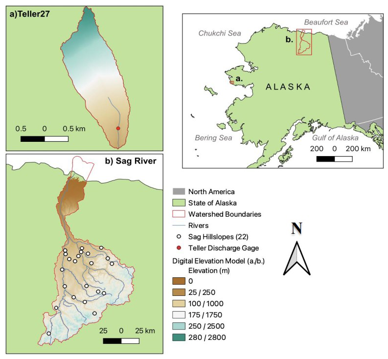
Figure 1 Map of the (a) Teller27 and the (b) Sag River sites, and inset map of Alaska with sites indicated with red boxes. Detailed site maps (a) and (b) include watershed boundaries (red), rivers (blue), Sag River hillslopes (white dots, 22), the Teller27 discharge gauge (red dot), and the Digital Elevation Models (DEMs) for each site. The 2.5 km² Teller27 site, being much smaller and with much more limited elevational range than the Sag River site, is 10 times smaller than the Sag River basin elevational range (see legend). Sag hillslopes (22) are not found on the lower elevation North Slope coastal plain, below 250 m.

The second study area is the Teller watershed, a 2.5 km² drainage basin located approximately 27 miles from Nome on Teller Highway, located on the Seward Peninsula of Alaska (hereafter referred to as Teller27, Fig. 1b). Compared to the cold and dry climate of the Sag River basin, the Teller27 site experiences a warmer and wetter climate. The Sag site receives over twice the annual snowfall of Teller27, while the Teller27 site is 7–8 °C warmer on average (Gao and Coon, 2022). The watershed is situated in a landscape of rolling hills underlain by discontinuous permafrost, where thaw depth varies considerably across slope positions and is strongly influenced by soil and vegetation cover. The land cover is dominated by moist tundra ecosystems, including mosses, dwarf shrubs, and patches of willow along riparian zones. Soils generally consist of an organic-rich surface horizon underlain by silty to loamy mineral substrates. Streamflow measurements were collected at the Teller27 watershed river outlet (Busey et al., 2019) from 2016–2023. For additional climate, snow, subsurface properties, and permafrost at the Teller27 site, refer to Bennett et al. (2022), Jafarov et al. (2018), Léger et al. (2019), Thaler et al. (2023), and Wang et al. (2024).

3.2 Numerical Experiment Design

Our experimental design for this work consists of three main steps as follows. First, results from detailed ATS simulations at the Sag River basin were compared to ELM's runoff parameterization schemes. Specifically, ATS-simulated thaw depth, water table depth, and ice content were used in ELM's parameterization Eqs. (1)–(4), and the results were then compared to ATS-simulated total discharges. Second, runoff coefficients derived from the Sag site were implemented into ELM's source code and tested for transferability at the Teller27 site, without the need for additional ATS simulations. Third, ELM simulations at the Teller27 site were evaluated directly against observed streamflow data from the Teller watershed to assess the performance and generalizability of the adjusted runoff coefficients.

The ATS model was implemented to simulate local-scale hillslope hydrological processes at the Sag River site only. Meteorological forcing data for this region are sourced from the Daymet version 4 dataset (Thornton et al., 2020), developed at a daily timestep. ATS modeling follows three steps. First, a soil column with an initial temperature above freezing was subjected to bottom-up freezing by imposing a constant temperature of −10 °C at the bottom boundary until a steady-state frozen soil profile was formed. In this stage, only the subsurface flow-energy processes were included. The resulting pressure and temperature profiles were then used to initialize spin-up runs for each hillslope model until a cyclically steady state was achieved. During the spin-up phase, the full physics system was applied, including surface and subsurface thermal flow as well as surface energy balance processes, using smoothed meteorological forcings. Each cyclically steady hillslope was then used as the initial condition for transient simulations driven by real forcings. For all hillslope simulations, the bottom boundary temperature was fixed at −10 °C. Closed boundary conditions were applied to all other subsurface and surface boundaries except at the surface outlet, where a seepage face boundary condition was applied. Both the column and hillslope models were represented with three soil layers: the top two organic soil layers (i.e., acrotelm, catotelm) and the bottom mineral layer. The thickness and properties of the soil layers for hillslopes were determined based on the corresponding land cover types according to O'Connor et al. (2020). The soil properties of each soil layer are listed in Table S2. The thermal conductivity representation followed Atchley et al. (2015). For further details on ATS model mesh generation, boundary conditions, model setup, and initialization, refer to Jan et al. (2020), Gao and Coon (2022), and Coon et al. (2022). We randomly selected 22 hillslope sites within the Sag River basin, ensuring representation across a range of slope, aspect, and drainage area, providing a basis for sensitivity analysis.

ELM was implemented to simulate subgrid hillslope hydrological processes specifically for the Teller27 watershed. We configured ELM at a spatial resolution of 0.5°, incorporating finer-scale surface and land use input parameters, but not recently developed features such as the topounit or elevation bands that represent sub-grid variability (Hao et al., 2022; Tesfa and Leung, 2017). ELM was driven by 1-hourly meteorological forcing data from ERA5-Land (Muñoz-Sabater et al., 2021), ensuring realistic and high-temporal-resolution atmospheric inputs. We used the Offline Land Model Testbed (OLMT) to standardize the ELM case setup and model spin-up (e.g., Sinha et al., 2023). Model spin-up proceeds through two phases after Thornton and Rosenbloom (2005): the first phase features accelerated biogeochemical cycling, while the second phase uses standard biogeochemical reaction rates. These spin-up phases are run for 260 and 200 years, respectively, to ensure vegetation and biogeochemistry have approached a steady-state condition before beginning a transient run that spans 1850–2024. To validate the runoff from ELM, we used the streamflow measurements collected at the gage. To evaluate the influence of soil property parameters on ELM-simulated runoff, a series of parameter sensitivity analyses was conducted. In each simulation, one parameter was perturbed by ±50 % from its default average value (ELM's surface and land use files are extracted from the global 0.5° resolution files), while the values of all other parameters were fixed.

3.3 ELM runoff parameterization evaluation

We constructed variable-width hillslope models for each of the 22 hillslope sites to represent both vertical and lateral dynamics and simulated the fully coupled cryo-hydrological processes using ATS. To facilitate comparison with ELM, we post-processed the ATS simulation outputs by averaging the surface and subsurface variables across ATS's multiple horizontal units (columns), preserving the number of vertical layers (rows, Fig. 2). This produced a 1D multi-layer (rows), single column profile that mimics ELM's 15-layer subgrid-scale structure. From this 1D multi-layer representation, key model variables such as maximum seasonally thawed depth of the upper soil layers above the permafrost (referred to as active layer thickness, ALT), surface water content, water table depth, soil moisture and ice content were extracted and used as inputs to ELM's runoff parameterization equations (Eqs. 1–4) to compute surface and subsurface runoff components. The resulting total runoff from ELM was then compared against the cumulative runoff stimulated directly by ATS. Figure 2 illustrates the overall workflow, including the extraction and processing of ATS's variables, the calculation of ELM runoff components, and the comparison with ATS's discharge accumulation at the outlet, as well as the averaging of ATS horizontal units to a 1D multi-layer representation. Layers can be of variable depth, as indicated in Fig. 2.

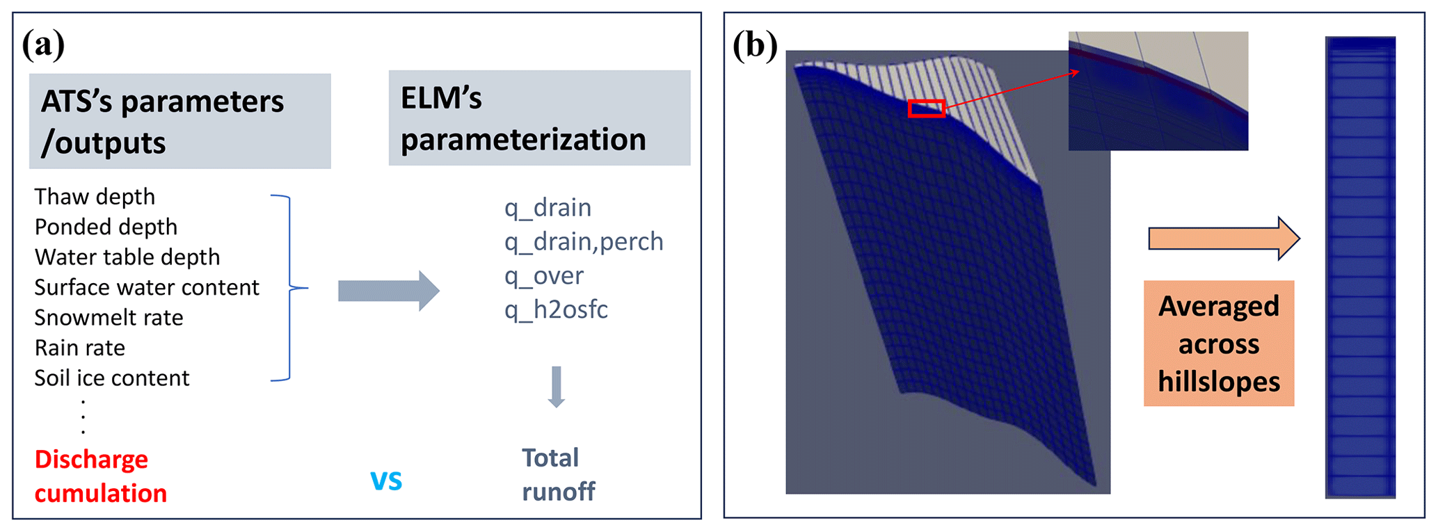
Figure 2 Map (a) Workflow for calculating ELM's total runoff, highlighting key variables, runoff components, and computational steps involved. (b) Averaging of ATS's simulation results, illustrating the transformation from high-resolution pseudo-2D ATS outputs averaged across all hillslopes, to simplified 1D ELM column representations.

To obtain the optimized runoff coefficients, we formulated objective functions that minimize the difference between the ATS-simulated runoff and a weighted sum of ELM's runoff components. The optimization was carried out using a constrained numerical minimization algorithm, with non-negativity bounds imposed on all coefficients. This procedure was conducted across multiple hillslope sites and under both annual and seasonal (warm–cold) conditions, resulting in site-independent adjusted coefficients for each case. To assess the performance of the optimized runoff coefficient and quantify the differences between them, three statistical metrics were calculated: root mean square error (RMSE), mean absolute error (MAE), and Nash–Sutcliffe efficiency coefficient (NSE). These metrics were selected as complementary evaluation measures following standard hydrological model assessment practices (Moriasi et al., 2007). RMSE emphasizes large errors and highlights peak mismatches, MAE reflects the average magnitude of deviations and is less sensitive to outliers, and NSE evaluates overall model efficiency relative to the observed mean. Together, they provide a balanced and robust assessment of ELM runoff performance. They are defined as follows:

$$\begin{array}{}\text{(11)}& {\displaystyle }\mathrm{RMSE}\left(c_{\mathrm{1}},c_{\mathrm{2}},c_{\mathrm{3}},c_{\mathrm{4}}\right)=\sqrt{{\displaystyle \frac{\mathrm{1}}{n}}{\sum }_{i=\mathrm{1}}^n{\left(y_{\mathrm{i}}-{\widehat{y}}_{\mathrm{i}}\right)}^{\mathrm{2}}}\text{(12)}& {\displaystyle }\mathrm{MAE}\left(c_{\mathrm{1}},c_{\mathrm{2}},c_{\mathrm{3}},c_{\mathrm{4}}\right)={\displaystyle \frac{\mathrm{1}}{n}}{\sum }_{i=\mathrm{1}}^n\left|y_{\mathrm{i}}-{\widehat{y}}_{\mathrm{i}}\right|\text{(13)}& {\displaystyle }\mathrm{NSE}\left(c_{\mathrm{1}},c_{\mathrm{2}},c_{\mathrm{3}},c_{\mathrm{4}}\right)=\mathrm{1}-{\displaystyle \frac{{\sum }_{i=\mathrm{1}}^n{\left(y_{\mathrm{i}}-{\widehat{y}}_{\mathrm{i}}\right)}^{\mathrm{2}}}{{\sum }_{i=\mathrm{1}}^n{\left(y_{\mathrm{i}}-{\stackrel{\mathrm{‾}}{y}}_{\mathrm{i}}\right)}^{\mathrm{2}}}}\end{array}$$

where y_i and ${\stackrel{\mathrm{‾}}{y}}_{\mathrm{i}}$ represent the ATS simulated value and its average value, respectively; ${\widehat{y}}_{\mathrm{i}}=c_{\mathrm{1}}{q}_{\mathrm{drain}}+c_{\mathrm{2}}{q}_{\mathrm{drain},\mathrm{perch}}+c_{\mathrm{3}}{q}_{\mathrm{over}}+c_{\mathrm{4}}{q}_{\mathrm{h}\mathrm{2}\mathrm{osfc}}$ is the calculated (or optimized) value based on ELM's equations. The coefficients c₁, c₂, c₃, and c₄ are weighting factors used to evaluate the relative contribution of each component. In the non-adjusted case, all four coefficients are set to 1.0, directly summing all runoff components. In the adjusted case, the coefficients are optimized through regression against the ATS-simulated runoff to best match the observed behavior. n is the number of annual or seasonal cumulative runoff values used in the comparison.

4 Results

4.1 Evaluation of the runoff schemes in ELM

ELM runoff results were evaluated in comparison with ATS's drainage at the outlet. In the plots below, we compared the annual and seasonal total cumulative runoff using both adjusted and non-adjusted coefficients c_i, under a variety of conditions across different hillslope sites (e.g., forcings, slope, ALT, etc.). The three columns in Fig. 3 correspond to different ELM parameterization cases: (1) unadjusted coefficients, (2) annually optimized coefficients, and (3) seasonally (warm–cold) optimized coefficients. The three rows represent different color-coded variables: slope (top), ALT (middle), and total precipitation (bottom).

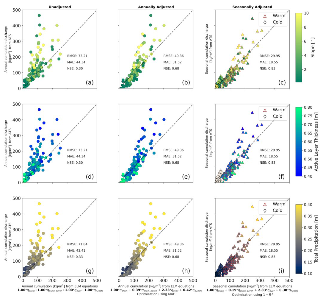
Figure 3 Comparison of cumulative total runoff between ATS and ELM models under various hillslope conditions. The different colors represent slope (a–c), active layer thickness (d–f), and total precipitation (g–i). Columns (from left to right) correspond to different coefficient settings in ELM: unadjusted (a, d, g), annually adjusted (b, e, h), and seasonally adjusted (c, f, i). The results are displayed for different runoff parameterization coefficients (as indicated on the x axis) in ELM and compared against ATS-simulated runoff.

It can be seen that ELM's annual total cumulative runoff is generally smaller than ATS's runoff when using unadjusted runoff coefficients, with an NSE of 0.30 (Fig. 3a). However, when adjusted coefficients are applied, the two models show much better agreement, achieving an NSE of 0.68 when adjusted based on annual discharge (Fig. 3b) and 0.83 when optimized using separate adjustments for the warm and cold periods (Fig. 3c). The seasonal total cumulative runoff is calculated for the warm season (May to August) and cold season (September to April) within the calendar year. This improved alignment in the seasonal total cumulative runoff is also reflected in performance metrics, with the RMSE, MAE, and NSE increasing by 39 %, 41 %, and 22 %, respectively, over the total runoff without adjusted coefficients, respectively.

The total runoff during the cold season is normally lower than that of the warm season. This is primarily because when the ground is fully frozen, overland flow (q_over) becomes the only dominant component of total runoff, which occurs due to excess meltwater from snow after limited vertical infiltration. As shown by the diamond symbols in Fig. 3c, f, and i, ELM's results are generally well-aligned with ATS's drainage during cold seasons, though some values are slightly lower. In the cold season, no active layer exists, whereas it does exist during the warm season. Cold-season runoff on steeper slopes tends to be lower, likely due to limited infiltration in frozen soils, which reduces subsurface flow pathways. In contrast, during the warm season, total runoff generally increases with slope, as shown in Fig. 3c, likely due to enhanced overland flow and faster hydrological response. Despite this trend, the runoff alignment in the seasonal total runoff (Fig. 3c) remains better compared to the total annual (Fig. 3b). This indicates that runoff differences between the two models cannot be fully explained by variations in slope, highlighting the influence of additional factors such as model parameterizations and physical processes.

By carefully examining the results with the adjusted coefficients in Fig. 3b, we observed that ELM performs well in representing lower slopes compared to the ATS benchmark, with a few exceptions. On steeper slopes (> 8°), ELM predicts lower runoff values than ATS, with differences reaching up to 150 kg m⁻². Interestingly, ELM also underpredicts runoff on shallower slopes (< 2°), suggesting that runoff differences between the two models are influenced by more than just slope. This variation could arise from differences in how the two models handle topographic gradients, basin size, or spatial heterogeneity in climate forcings. Figure 3e highlights that ELM performs better with deeper ALT, likely because these active layers experience less freezing, allowing for increased water storage in the deeper thawed zones and reduced lateral drainage. Figure 3h reveals a strong relationship between total cumulative runoff and precipitation, and ELM generally captures lower precipitation events more accurately, leading to correspondingly lower total runoff. As expected, Fig. 3i reveals a clear trend between warm-season total runoff and precipitation magnitude. However, ELM tends to underpredict runoff under higher precipitation conditions. This underscores the critical role of climate forcing data in shaping model performance and highlights ELM's sensitivity to precipitation variability.

To better understand these findings, it may be important to consider spatial variations in terrain landforms (e.g., concave vs. convex) across the modeled hillslopes, as well as alternative hillslope representations through structural formulations (e.g., Swenson et al., 2019; Lawrence and Swenson, 2024). In addition, these watersheds span a broad latitudinal range (approximately 68 to 70° N), which likely introduces considerable climatic and topographic variability. For example, steeper slopes can promote rapid surface runoff, while gentler slopes with deeper thawed layers may enhance water retention and reduce lateral drainage.

This improved alignment between ELM and ATS's annual total cumulative runoff is also evident in time series comparisons of total runoff from a selected hillslope, shown in Fig. 4, both with and without adjusted coefficients. Figure 4a illustrates the results using the unadjusted coefficients, where ELM underestimates runoff peaks and exhibits a relatively weak correlation with ATS discharge. The RMSE, MAE, and NSE values (0.55, 0.22, and 0.48, respectively) indicate moderate agreement but suggest room for improvement, particularly in capturing peak runoff events. Figure 4b shows the impact of applying annually adjusted coefficients, which improves model performance, as reflected by reduced RMSE (0.51) and MAE (0.19), along with a higher NSE (0.56). The adjusted coefficients result in better agreement during high-runoff periods, though some discrepancies remain in capturing the full variability of runoff responses. Figure 4c presents the results with seasonally adjusted coefficients, which yield the best overall performance among the three cases. The RMSE and MAE decrease further to 0.46 and 0.18, respectively, while the NSE increases to 0.64, demonstrating a stronger correlation between ELM and ATS runoff. The seasonal adjustment appears to enhance the model's ability to capture the timing and magnitude of runoff peaks (see Fig. 4d), particularly during snowmelt periods. However, some deviations remain, likely due to limitations in parameterizing snowmelt-driven surface flow and subsurface hydrological interactions in ELM.

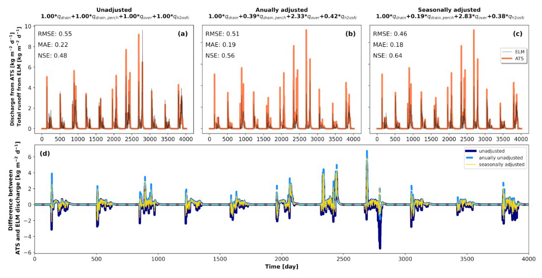
Figure 4 Time series comparison of total runoff between ATS and ELM for a typical hillslope with an average slope of 6.6°, a watershed area of 2.43 km², and the ALT ranging from 0.43 to 0.59 m. Results are shown with (a) unadjusted coefficients, (b) annually-adjusted coefficients, and (c) seasonally-adjusted coefficients.

These results highlight the importance of refining runoff coefficients and incorporating seasonal variations to improve the predictive capability of ELM, particularly in Arctic environments where snowmelt dynamics play a dominant role in runoff generation. In general, better alignment is observed when ATS's cumulative runoff remains below a certain threshold, such as 15 kg m⁻² d⁻¹. For larger runoff, ELM tends to underpredict total runoff, indicating limitations in its ability to represent higher runoff scenarios accurately.

4.2 Teller27 watershed evaluation

The improved ELM runoff coefficients were evaluated using observed streamflow data from the Teller27 watershed, spanning 2016–2019 (Busey et al., 2019). Results in Fig. 5 indicate that the adjusted coefficients significantly enhance the agreement between ELM-simulated runoff and observations. The unadjusted coefficients consistently underpredict runoff, with the largest discrepancy observed in 2016 (ELM: 374.66 kg m⁻², observed: 648.25 kg m⁻²). Both annually and seasonally adjusted coefficients reduce this gap, with the seasonally adjusted coefficients providing better performance, particularly in years with greater interannual variability in precipitation and thaw depth.

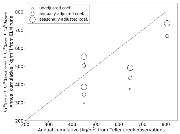
Figure 5 Comparison of cumulative annual total runoff between ELM-simulated and observed data at the Teller27 watershed, Alaska, from 2016 to 2019. Symbol sizes represent ELM results using unadjusted coefficients, annually adjusted coefficients, and seasonally adjusted coefficients.

Figure 6 presents the outcomes of the parameter sensitivity experiments, illustrating how changes in land surface properties influence simulated total runoff. It can be seen that total runoff is relatively insensitive to variations in surface soil properties such as clay, sand, and organic matter content, suggesting that soil texture and composition play a secondary role in controlling runoff dynamics within the model. Simulated runoff totals under these parameter perturbations remained within a relatively narrow envelope, regardless of whether baseline or optimized runoff coefficients were applied. This occurs because runoff is most due to overland flow during the spring snowmelt, when the ground is still frozen. These differences were notably smaller than the variations observed across different years or watersheds. The broader implications of these findings are further discussed in Sect. 5.2.

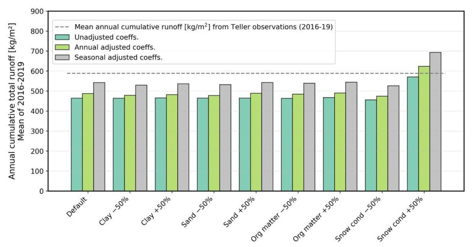
Figure 6 Variations in annual cumulative total runoff from ELM simulations at the Teller27 watershed, Alaska for the mean of all years (2016–2019). Different bars groupings along the x axis illustrate scenarios where parameters are reduced or increased from their default average values in ELM's soil physical property and snow thermal conductivity. Bar colours represent results with unadjusted coefficients (teal), annually adjusted coefficients (green), and seasonally adjusted coefficients (grey). The mean annual cumulative runoff from Teller observations (mean all years 2016–2019) is given in the dashed line.

Figure 7 shows a temporal comparison of weekly and monthly total runoff, while Table 1 quantifies performance using RMSE, MAE, and NSE metrics. The adjusted coefficients yield lower RMSE and MAE values and higher NSE scores than the unadjusted coefficients, confirming their effectiveness, despite being derived from a study site some distance from the Teller27 watershed. These results clearly demonstrate that ELM's subgrid-scale runoff scheme performs well at the monthly timescale, but struggles to capture sub-monthly (e.g., weekly) runoff variability. Although ELM's total runoff is of the same order of magnitude as the observed discharge at Teller creek, discrepancies arise during specific events. Notably, spikes in runoff occur during rapid snowmelt in early spring due to ponded surface water, and the baseflow during recession periods are poorly simulated.

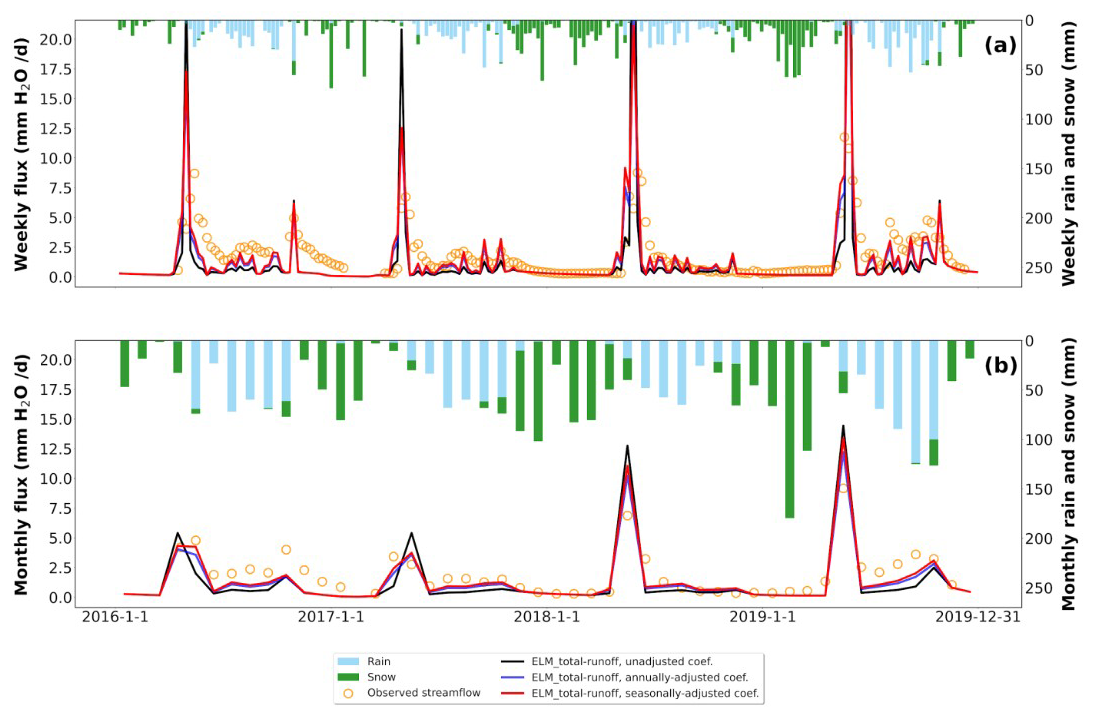
Figure 7 Comparison of ELM-simulated (a) weekly and (b) monthly total runoff with observed data at the Teller27 watershed, Alaska. Simulated results are displayed using different runoff parameterization coefficients in ELM, represented by distinct colored lines. Rain and snow precipitation are shown as bar plots using the top x axis (time) and left y axis (mm) in both subplots.

Table 1 Performance metrics (RMSE, MAE, and NSE) for ELM-simulated total runoff compared to observed streamflow across all temporal scales (daily, weekly, and monthly) at the Teller27 watershed, Alaska.

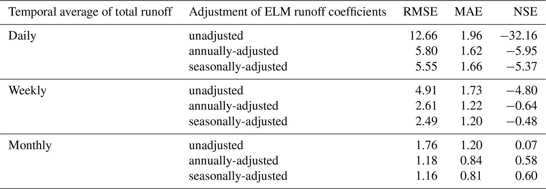
The weekly average results (Fig. 7a) reveal significant discrepancies in runoff peaks with unadjusted coefficients, while those biases are reduced by the simulations with adjusted coefficients. This may be due to large peak flow simulated during snowmelt in ELM that is not represented in the observations, thus flows throughout the rest of the summer are too low in the simulations. We believe that this response may be occurring due to a frozen active layer that leads to fast runoff that is not observed in the hydrological records. While we observed this overestimate of flow peaks, the seasonally adjusted coefficients still perform better in capturing both the timing and magnitude of runoff peaks, perhaps because the seasonal coefficients adjust for some attenuation of runoff. The monthly results (Fig. 7b) show improved agreement with observed data during high runoff periods, particularly those driven by snowmelt and seasonal precipitation. This is likely because the monthly results accumulate flow responses over longer periods of time, accounting for and spreading out this large peak flow runoff response that was incorrectly simulated at the weekly time scale. For example, at the monthly scale, NSE improves markedly from 0.07 with unadjusted coefficients to 0.58 and 0.60 with annually and seasonally adjusted coefficients, respectively. These results highlight the efficacy of the adjusted coefficients and the critical role of incorporating seasonal variability into runoff parameterization for improving ELM's performance.

5 Discussion

Intercomparison studies to consider differences and similarities between a land surface scheme to a physically-based model are useful because they allow for quantitative evaluation of each model and its performance for different components of the hydrologic cycle. The technique applied here was to extract the land surface parameterization schemes and evaluate them within a fine-scale, physics model, to consider the total cumulative runoff from the land surface scheme (y^ELM_runoff) and compare it with the physics model estimates (y^ATS_runoff). This novel approach allowed us to focus on the formulations over other interacting effects that may have potentially obscured the results. We were then able to make an estimate of runoff coefficients that could be applied to improve the match between the physics-model and the land surface model. These coefficients, when applied to a small watershed located in sub-arctic Alaska, improved the land surface model (y^ELM_runoff) significantly, suggesting that this approach may allow for fine-tuning of runoff within similar systems. Overall, further research is needed to determine how flexible these coefficients are; however, this work was foundational in that it provided a novel approach to both model intercomparison as well as for model improvement.

A sensitivity analysis conducted as part of this study identified that soil properties may exert less influence on the runoff dynamics in the land surface model than snow accumulation and melt processes, as well as subsurface thermal hydrology. This finding links this component of our research to investigations into snow processes and model improvement in these same systems (e.g., Bennett et al., 2022; Clark et al., 2015). It is clear that to improve runoff processes within permafrost dominant systems, a holistic approach to understanding the system is required to determine the key processes and model components that require adjustment. This study provided an initial enquiry into this process that developed the foundation for our work towards improving the Earth system model for these Arctic systems.

5.1 Differences in simulated runoff from representative hillslopes

The apparent mismatch between y^ELM_runoff and y^ATS_runoff results from 22 representative hillslopes in the Sag River basin warrants a critical examination. However, such evaluations must consider the inherent differences between the two models. Several factors could contribute to these differences. First, a key distinction between ATS and ELM is their treatment of runoff generation processes. ATS implicitly simulates variably saturated flow, lateral subsurface flow and transport, and dynamic freeze-thaw cycles in a high-resolution 3D domain (Painter et al., 2016; Coon et al., 2020). In contrast, ELM utilizes parameterized equations to represent subgrid-scale heterogeneities, which are not expected to fully capture the complexity of permafrost hydrology (Bisht et al., 2018; Xu et al., 2024). This averaging process that reduces a 3D system into a pseudo-3D system in ATS can represent a loss of spatial variability in hydrological processes, particularly in heterogeneous permafrost regions where local-scale topography and subsurface heterogeneity play a critical role in runoff generation (Zhao and Li, 2015; Abolt et al., 2024). This simplification can also lead to discrepancies in how surface and subsurface runoff are partitioned (Liao et al., 2025), particularly in regions with high spatial variability in soil moisture, ice content, and thaw depth. For instance, ELM may under- or over-predict runoff during high precipitation events (see Fig. 5) compared with the spatially resolved, physics-based implementation in ATS.

Secondly, although y^ATS_runoff is treated as the benchmark in this study, it is not without uncertainties. The accuracy of y^ATS_runoff simulations depends on input data such as soil properties, meteorological forcings, and initial conditions, all of which contain inherent uncertainties (Harp et al., 2016; Jafarov et al., 2018; Zhang et al., 2023; Huang et al., 2022, 2024). In permafrost landscapes, soil heterogeneity is particularly difficult to characterize, and small variations in soil thermal and hydrological properties can lead to substantial differences in runoff predictions (Decharme et al., 2013; Vereecken et al., 2022).

Additionally, the accuracy of y^ELM_runoff predictions is highly dependent on the parameterization of surface hydrological processes. Although optimized coefficients have been implemented to improve agreement with y^ATS_runoff, these parameterizations may still inadequately capture the nonlinear interactions between infiltration, permafrost thaw, and lateral flow (Swenson et al., 2012; Liao et al., 2025). This issue is particularly relevant in ice-rich permafrost terrains, where abrupt changes in thaw depth and active layer dynamics can lead to nonlinear responses in runoff generation (e.g., Hinzman et al., 2022). The lack of explicit lateral flow representation in ELM further limits its ability to capture runoff redistribution processes that are well-resolved in ATS simulations.

Another factor that may contribute to the mismatch is the difference in how the two models resolve seasonal freeze/thaw processes, especially under varying precipitation and thawing conditions. Runoff generation in permafrost regions is highly sensitive to seasonal thawing and freezing dynamics, as well as precipitation regimes (e.g., Zhang et al., 2010; Guo et al., 2025). In particular, mismatches may arise during transitional periods such as spring snowmelt, when small differences in temperature and soil conditions can lead to substantial variations in runoff production.

Understanding these potential differences is crucial for interpreting the model responses and guiding future ELM model improvements. Addressing the uncertainties in ATS and refining the transformation of parameterization schemes between models could reduce these mismatches. Similarly, enhancing ELM's parameterization by incorporating insights from ATS simulations, such as better representation of lateral flow and freeze-thaw processes, could lead to improved alignment with ATS and more accurate predictions in Arctic environments under a changing climate.

5.2 Sensitivity and uncertainties of model performance to land surface parameters in ELM

The sensitivity analysis assessed the impact of various surface and subsurface parameters, including soil properties (clay, sand, and organic content) and snow thermal conductivity, on the simulated total y^ELM_runoff. Understanding the sensitivity of y^ELM_runoff simulations to these parameters is crucial for improving hydrological predictions in permafrost regions, where land surface processes interact with freeze-thaw dynamics in complex ways (Bisht et al., 2018; Walvoord and Kurylyk, 2016).

The limited sensitivity of total y^ELM_runoff to soil property variations observed in our ELM simulations raises important implications for land surface model development. Previous studies have shown that soil texture can strongly affect bidirectional water exchange between groundwater and the soil during freeze–thaw transitions (e.g., Xie et al., 2021; Huang and Rudolph, 2023; Yang et al., 2025). However, our findings suggest that these processes may have less influence on annual runoff generation in permafrost regions. This discrepancy may be explained by the dominant role of snowmelt dynamics and shallow subsurface hydrology in controlling surface runoff. In permafrost-dominated landscapes, runoff generation is often driven by the timing and intensity of snowmelt, seasonal freeze–thaw cycles, and the spatial distribution of near-surface permafrost. These factors likely outweigh the direct effects of variations in soil grain size or organic matter content (e.g., Swenson et al., 2012). The presence of an impermeable permafrost layer beneath the active layer restricts deep infiltration and causes excess water to remain near the surface, limiting the direct impact of soil properties on runoff partitioning. Similar findings have been reported in other permafrost hydrology studies, where hydraulic conductivity and soil texture exert minimal influence on runoff formation compared to freeze-thaw dynamics and snowmelt timing (e.g., Zhang et al., 1999; Walvoord and Kurylyk, 2016). However, further investigation is needed to evaluate whether subsurface water redistribution, active layer depth variability, and lateral flow dynamics could play a more significant role in influencing ELM's runoff performance.

In contrast to soil parameters, snow thermal conductivity exhibits a strong influence on simulated runoff, demonstrating its critical role in shaping hydrological responses in Arctic environments. An increase in snow thermal conductivity enhances heat transfer within the snowpack, leading to earlier and more rapid snowmelt. This, in turn, alters the seasonal timing of water availability and increases runoff magnitudes during peak melt periods (Musselman et al., 2017). Higher thermal conductivity results in faster warming of the snowpack, reducing the buffering effect of snow insulation and exposing the underlying soil to greater temperature fluctuations. This phenomenon has been observed in field studies, where changes in snow properties significantly impact the timing and magnitude of spring runoff (Würzer et al., 2016; Liljedahl et al., 2016). The results in Fig. 6 suggest that accurate representation of snow properties is essential for improving y^ELM_runoff predictions in permafrost landscapes. Over- or under-estimating snow thermal conductivity could lead to systematic biases in modeled y^ELM_runoff timing, potentially affecting the accuracy of hydrological assessments in Arctic watersheds.

Collectively, these findings reinforce the critical role of snowmelt-driven hydrological processes in shaping runoff dynamics in permafrost landscapes and illustrate key sensitivities within ELM's runoff parameterization. The results suggest that ELM's performance is particularly influenced by representations of snow accumulation and melt processes, as well as subsurface thermal hydrology. In particular, sensitivity to snow density, thermal conductivity, and freeze–thaw transitions points to the value of incorporating physically based formulations that capture snowpack variability (e.g., Bennett et al., 2022; Lackner et al., 2022; Tao et al., 2024; Wang et al., 2024) and lateral subsurface flow (e.g., Swenson et al., 2012; Liao et al., 2025). These process-level influences appear to exert a stronger control on y^ELM_runoff behavior than surface soil properties alone, underscoring their importance in cold-region hydrology and land surface modeling.

5.3 Implications for improving runoff parameterization coefficients in land surface models

Hydrological runoff-related parameters in land models are often calibrated against the observed streamflow data (e.g., Niu et al., 2007; Li et al., 2013), which can be limited or unavailable in remote permafrost regions. This study introduces a novel evaluation framework, which shifts the traditional paradigm of directly comparing coarse-scale land surface models to fine-scale physics-based models, by deriving optimized runoff coefficients by leveraging high-fidelity simulations from the integrated surface/subsurface hydrological simulators such as the ATS. These optimized coefficients are then incorporated into the land surface model, allowing for physics-informed improvements without direct site-based calibration. This approach offers a process-oriented alternative to conventional calibration, providing an avenue for improving parameterizations in data-scarce regions.

A key implication of this framework is its potential transferability across diverse Arctic watersheds. In this study, coefficients derived from the Sag River hillslopes were applied to the Teller27 watershed without additional tuning, resulting in significantly improved y^ELM_runoff performance at monthly and seasonal scales. One possible reason for this is that while these two systems are located in very different environments and some distance from each other, they are similar in that both exhibit moderately graded slopes and elevations, vegetation of grasses and shrubs, and both have some degree of permafrost (albeit discontinuous permafrost in Teller27). However, in this iteration of ELM, most of the sub-grid variability within these features are not represented, despite their importance to the influence of snowmelt runoff and other water balances (e.g., Beer, 2016; Shirley et al., 2025). This demonstration suggests that physically guided coefficients obtained through fine-scale process-resolving models may be generalized to other Arctic catchments with similar characteristics, offering a possible strategy for parameter refinement in Earth system land models at coarse scales. Such transferability is especially valuable for land model intercomparison projects that seek robust parameterizations applicable across diverse permafrost regions (e.g., Clark et al., 2015; Lawrence et al., 2019; Fan et al., 2019). However, more research is required to determine the extent of this transferability. Future applications of this approach at permafrost sites across the pan-Arctic, which is part of the next phase of this project, could further enhance the robustness and generalizability of this framework.

Our coefficient-calibration approach complements, but also differs from, the representative hillslope approach developed for the CLM (Swenson et al., 2019; Lawrence and Swenson, 2024). In CLM's representative hillslope approach, intrahillslope lateral subsurface flow is explicitly represented and scaled through representative hillslopes that account for slope, aspect, and lateral redistribution of water. This structural modification allows the model to capture lateral connectivity in a process-based manner without requiring high-resolution benchmarks. By contrast, our method leverages physics-based ATS simulations to calibrate and optimize runoff coefficients in ELM and then evaluates their transferability across sites. Whereas the CLM approach introduces structural reformulations of runoff schemes, our framework focuses on refining existing parameterizations through calibration against physics-based permafrost models. Taken together, these strategies represent complementary pathways for advancing runoff representation in permafrost regions and for bridging local-scale hydrological processes with land surface components of Earth system models. At the same time, ELM has recently developed an improved subgrid hillslope hydrologic connectivity that represents lateral water movement across topographic units (topounits) within a gridcell. This new implementation shares similarities with the CLM hillslope approach. Future evaluation of the runoff performance of that parameterization alongside our coefficient-calibration framework will be an important next step toward improving parameterization and scaling of hydrological processes in ELM. Such integration of coefficient calibration, representative hillslope formulations, and the new subgrid framework will be essential for capturing hydrological variability across diverse permafrost landscapes and for improving the predictive fidelity of Earth system land models under changing Arctic climate conditions.

6 Limitations and future work

Based on our analysis and discussion, we acknowledge several limitations that may be further improved in future studies:

Simplified watershed representation. The hillslopes used for ATS simulations in the Sag River basin are pseudo-2D variable-width simplifications of the 3D landscapes, which do not fully capture the heterogeneity of real Arctic landscapes, such as ice-wedge polygons, thermokarst features, and microtopographic variations. Future studies should incorporate many more diverse landscapes (up to hundreds of hillslope models) and ensure identical topographic representations across both models.

Transferability evaluation. The optimized runoff coefficients were derived from ATS simulations of Sag River hillslopes and then directly applied to the Teller Creek watershed without site-specific adjustments. This transferability was only evaluated at a single site (Teller27), further evaluation across diverse Arctic watersheds with long-term streamflow measurements is needed to build broader confidence in the generalizability of the approach. Moreover, because seasonal variability plays a key role in runoff generation, this approach may work reasonably well for colder Arctic regions but may be less applicable to sub-Arctic environments.

Limited consideration of lateral flow and subsurface heterogeneity. This study primarily focused on ELM's grid-scale runoff generation, neglecting lateral water movement and groundwater interactions. In Arctic environments, lateral subsurface flow can play a crucial role in redistributing water across permafrost landscapes, affecting both surface runoff and baseflow dynamics in different land units, which will be evaluated in future work.

Limited assessment of meteorological forcing biases. While the parameterization in this study is based on state variables derived from ATS simulations, rather than directly on precipitation or other forcings, model performance in applications such as the Teller Creek test can still be sensitive to uncertainties in meteorological inputs. In high-latitude regions, sparse station coverage and undercatch issues can introduce substantial uncertainty in precipitation, temperature, and radiation datasets. Future work should assess how these uncertainties propagate through the model and influence runoff simulations under different forcing scenarios.

7 Conclusions

We evaluated a land surface model's runoff parameterization using detailed fine-scale physics-based simulations of 22 hillslopes in the Sag River basin and identified empirical adjustments that improve the runoff parameterization. Seasonal optimization of these coefficients improved the model's ability to capture hydrological variability at monthly scales, particularly in snowmelt-driven runoff processes. The adjusted parameterization improved ELM simulated runoff from the Teller27 watershed. That demonstration of transferability of the adjusted parameterization is encouraging but needs further study across diverse Arctic catchments. Sensitivity analysis revealed that runoff in ELM is largely insensitive to soil properties but highly sensitive to snow thermal conductivity, underscoring the importance of accurate snow process representation in permafrost regions. These findings demonstrate the value of spatially resolved fine-scale simulators from physics-based models as benchmarks for refining land surface models and highlight the need for process-specific parameterization improvements in hydrological runoff schemes of land surface models.

Despite these advancements, challenges remain in capturing subsurface hydrological processes, including lateral flow, permafrost thaw dynamics, and active layer variability, which are critical for Arctic runoff simulations. Future improvements should focus on incorporating water redistribution within an ELM gridcell due to lateral flow, refining subgrid-scale hydrological parameterizations, and evaluating model updates across diverse Arctic catchments. By addressing these gaps, land surface models could achieve more accurate runoff predictions, ultimately enhancing their utility for climate impact assessments and water resource management in permafrost regions.