
the Creative Commons Attribution 4.0 License.
the Creative Commons Attribution 4.0 License.
 | 19 Nov 2026
An antiplane shear model for evaluating shear-margin stability (Ortholine v1.0)

Cooper W. Elsworth
Neelanjan Akuli
The lateral boundaries of ice streams and glaciers, commonly referred to as shear margins, play a key role in the mass balance of ice sheets. In glaciers, shear margins are often controlled by topography, whereas in ice streams they are inherently dynamic and can migrate. Margin migration alters the width of fast-moving ice and thus the force balance that controls ice speed and mass loss. Quantifying whether a shear margin is stable or prone to migration is hence important for estimating the future mass balance, but requires understanding the processes governing its current position. Numerous englacial and subglacial processes may contribute, including shear heating, fabric development, basal topography, lithology, and hydrology. Although the potential importance of these processes has been established, we currently lack models aimed at evaluating their relative importance at a specific field site and we aim to fill this gap. Here, we introduce “Ortholine”, an antiplane-shear free-boundary model developed to evaluate the relative importance of different englacial and subglacial processes in controlling a specific shear-margin location. Ortholine evaluates the relative importance of subglacial lithology, subglacial hydrology including channelized versus distributed drainage, basal topography and ice overburden, and englacial temperature through shear heating, while processes such as fabric development lie outside its current scope. By focusing on the cross-sectional force balance of ice streams, Ortholine complements commonly used flow-line models. After deriving and verifying Ortholine, we outline the four key steps for applying it to a field site, using Institute Ice Stream in the Weddell Sea Sector, Antarctica, as a proof-of-concept. We have selected Institute Ice Stream as an example, because of its intermediate complexity and the sufficient availability of field data to guide the model setup. Applying Ortholine at Institute, we find that spatial association alone is not a reliable indicator of the controlling process: the western shear margin is co-located with a topographic trough, yet our simulations indicate that a meltwater channel in that trough, rather than the topography itself, is the important control.
- Article
(8008 KB) - Full-text XML
- BibTeX
- EndNote


Ice streams and glaciers together account for the majority of mass loss from the Antarctic continent (Bamber et al., 2000). Their mass loss depends not only on the speed of the ice, but also on the width of the fast-flowing zone, which is set by the position of the shear margins (Raymond, 1996). Migration of a shear margin therefore changes the width of fast-moving ice and, with it, the discharge, so that shear-margin position directly affects the mass balance. Observations show that shear margins can move, either gradually (Harrison et al., 1998; Bindschadler and Vornberger, 1998; Echelmeyer and Harrison, 1999; Clarke et al., 2000) or abruptly (Catania et al., 2006). It is less clear how commonly shear margins move, partly because shear margins are difficult to pinpoint on satellite data due to heavy crevassing, and partly because migration rates on the order of meters per year are challenging to resolve. If shear margins were to move, the consequences for sea-level rise projections could be significant because the outward motion of a shear margin not only increases the width, but also the speed of fast-moving ice (Raymond, 1996).
The puzzling variability of observed shear-margin behavior raises the question of what physical processes control shear-margin mobility and how these processes might be affected by evolving climatic conditions. Previous models have improved our understanding of how thermal (Schoof, 2004, 2012; Suckale et al., 2014; Perol et al., 2015; Haseloff et al., 2015) and hydrological (Perol and Rice, 2015; Platt et al., 2016; Elsworth and Suckale, 2016) processes at the base of the ice contribute to the stability of shear margins. However, most of these models consider only a single shear margin assuming symmetric and idealized ice streams sliding over a homogeneous bed, inspired by the Siple Coast Ice Streams that are characterized by low topography, complex subglacial hydrology and widespread sediment deposits (e.g., Perol et al., 2015; Suckale et al., 2014; Elsworth and Suckale, 2016).
Figure 1 highlights the location of the Siple Coast Ice Streams superimposed on the shear-strain rate field of the Antarctic Ice Sheet as estimated from Landsat 8 satellite data by Alley et al. (2018). It also shows several other locations where shear-margin properties are likely controlled by other physical processes than in the Siple Coast, ranging from topography at Lambert Glacier (Sanderson et al., 2023), to spatial variations in subglacial conditions at Institute Ice Stream (Siegert et al., 2016), and possibly a combination of all of these at Thwaites Glacier. Thwaites Glacier is particularly relevant, because it is a case where one shear margin might be more prone to migration than the other (MacGregor et al., 2013) and because of its prominent contribution to current sea-level rise (e.g., Holland et al., 2023).
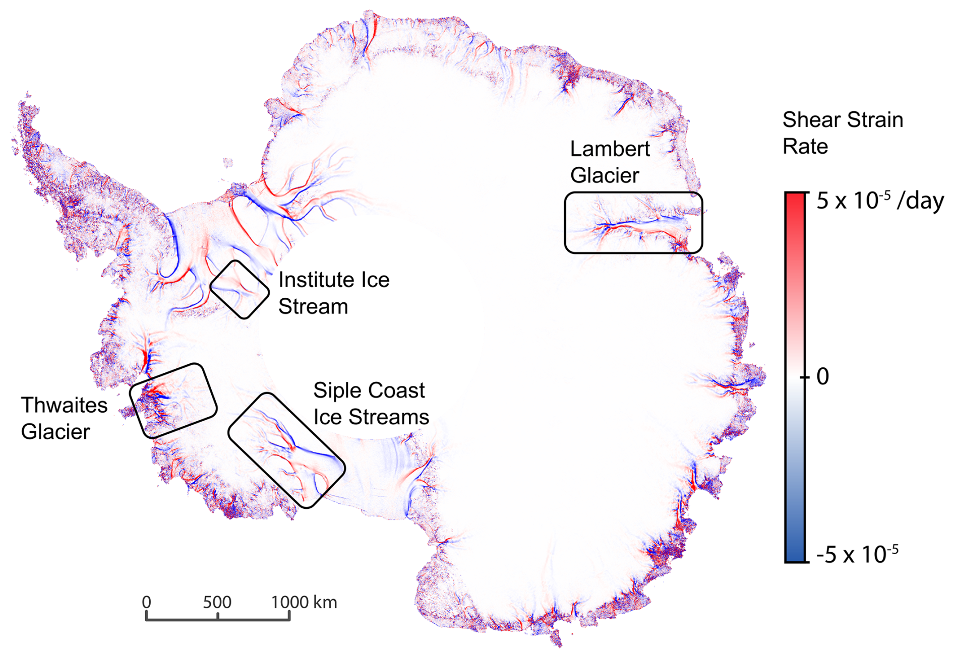
Figure 1Map of the shear strain rate estimated from the satellite-derived velocity field of the Antarctic ice sheet based on Landsat 8 satellite data by Alley et al. (2018). Superimposed are the locations where shear margins might be controlled by different physical processes.
The goal of this study is to advance our ability to evaluate the relative importance of different englacial and subglacial processes in controlling a specific shear-margin location by developing an easily portable model, “Ortholine”. Methodologically, Ortholine attempts to strike a balance between the appealing simplicity of idealized shear-margin models that have contributed to our theoretical understanding (e.g., Jacobson and Raymond, 1998; Schoof, 2004; Suckale et al., 2014; Haseloff et al., 2015; Perol and Rice, 2015; Elsworth and Suckale, 2016; Haseloff et al., 2019) and the inevitable complexity of the field sites for which we aim to assess shear-margin stability. We build on the cross-sectional, free-boundary formulation of Schoof (2006b, a), which allows us to determine the slipping regions at the ice-bed interface self-consistently from an integrated force balance.
Our model design is inspired by the scientific successes of simple flow-line models pioneered by Nye (1957) and widely adopted by the scientific community in the 1980s (e.g., Hooke et al., 1979; Morland and Johnson, 1980; Reeh and Paterson, 1988). Flow-line models neglect shear margins and thereby reduce a three-dimensional problem to plane flow along the main flow direction. A complementary point of view that allows for an explicit focus on shear margins is to assume antiplane shear and instead neglect longitudinal stresses (e.g., Jacobson and Raymond, 1998). By antiplane shear we mean the configuration in which the ice velocity is directed along the flow direction x, out of the cross-sectional plane, while its gradients are resolved within that cross-section; this is the standard usage in continuum mechanics and is distinct from the plane-flow assumption of flow-line models. The name of our model, “Ortholine”, is motivated partly by the orthogonal orientation of our model domain to the main flow line and partly by its conceptual orthogonality to flow-line models. Ortholine allows researchers to focus on an aspect of ice dynamics, the shear margin, that is neglected in flow-line models.
Previous antiplane shear models of shear margins simplify the domain as symmetric and assume a flat basal topography (Jacobson and Raymond, 1998; Schoof, 2004; Suckale et al., 2014; Perol and Rice, 2015; Haseloff et al., 2015; Elsworth and Suckale, 2016). Instead, we implement a body-fitted mesh using the Gmsh package (Geuzaine and Remacle, 2009) that can capture variable subglacial topography in the model domain. We also allow for heterogeneous basal conditions representative of perfectly plastic sediment behavior (Tulaczyk et al., 2000b; Kamb, 2001), velocity-strengthening hard rock sliding laws (Weertman, 1957), and regularized Coulomb sliding over hard rock (Schoof, 2005) while maximizing computational efficiency. Including these heterogeneities implies that the antiplane shear plane might not be identical to the cross-section of the ice stream. We have developed an accompanying algorithm to compute the appropriate model plane from surface velocities.
Although Ortholine is intended as a general framework that can be easily adapted to any given field site, we detail the steps to apply it for the case of Institute Ice Stream in the Weddell Sea Sector, Antarctica (see Fig. 1). Institute Ice Stream represents a field setting of moderate complexity that shares similarities with the Siple Coast, such as low overall driving stresses and a widespread unconsolidated sediment layer (Bingham and Siegert, 2007). Radio-echo sounding surveys map out a mildly varying topography and suggest the existence of a distinct transition between hardrock and saturated sediments beneath the ice stream (Siegert et al., 2016). From a dynamic point of view, Institute Ice Stream has attracted attention because it is located on a reverse-sloping bed with few pinning points (Bingham and Siegert, 2007; Ross et al., 2012), making it prone to the marine ice-sheet instability (Weertman, 1974; Thomas, 1979; Schoof, 2007; Jamieson et al., 2012).
We develop a thermomechanical model of an ice stream cross section oriented orthogonal to the flow line. Instead of prescribing the margin positions, we solve a free-boundary problem for the slipping portion of the bed based on an integrated force balance across the domain, following the derivation by Schoof (2006b). We formulate the governing equations of ice flow for three different subglacial boundary conditions representative of failing sediments, locked sediments, and hard-bed sliding. We then convert the free-boundary problem to a convex optimization problem and solve it through the Disciplined Convex Programming framework (Grant and Boyd, 2014).
2.1 Governing Equations
Our free-boundary model extends the mechanical model by Schoof (2006b) to include thermomechanical effects. To reduce the complexity of the 3-D geometry, we neglect variability in the downstream direction (), with the ice moving in the positive x direction, shown in the right-hand panel of Fig. 2. Neglecting downstream variability reduces the momentum balance to
with antiplane speed, u, temperature-dependent power-law coefficient, η(T), power-law exponent, n, ice density, ρ, gravitational acceleration, g, and surface slope, α. A typical non-Newtonian Glen's rheology would entail n=3 (Glen, 1955). We define , where A(T) is the Glen rate factor and E=4 is the enhancement factor. For n=3, .
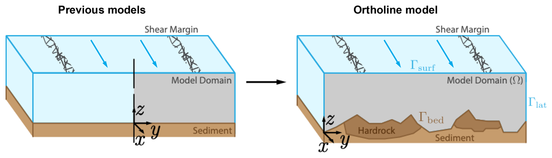
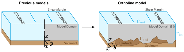
Figure 2Model domain of previous models as compared to Ortholine. Both model approaches neglect variability in the along-flow direction, x. Advancing on previous idealized models (left), Ortholine captures the entire width of the zone of fast-moving ice including both shear margins and allows for spatially varying lithology, subglacial hydrology and basal topography (right).
We neglect downstream variation in ice thickness and impose a stress-free surface,
where where n is the outward unit normal to the interface. Additionally, the domain has stress-free lateral bounds,
The basal traction at the bed,
takes one of two forms depending on whether the bed at a given location consists of saturated sediment or hard rock. We prescribe the partition of the bed into sediment and hard-rock regions from observations. The location of the rock–sediment transition and the degree to which this transition implies a significant difference in basal properties need to be assessed on a case-by-case basis. For example, we rely on the geophysical imaging by Siegert et al. (2016) to assign boundary conditions for Institute Ice Stream, Antarctica, as detailed below. The sediment boundary condition captures regions of water-saturated sediments that abide by Coulomb plasticity as observed experimentally (Tulaczyk et al., 2000b) with
dependent on effective pressure, , where σn is the overburden, p the pore pressure, Cf the friction coefficient and c the cohesion of the sediment.
For the portion of the subglacial bed that consists of hard rock, we assume that the basal traction follows a sliding law,
dependent on the downstream ice speed, u, to the power m. For the velocity-strengthening hard-rock cases below, we use ; the m=0 limit is retained for the Coulomb-sliding comparisons. The coefficient β is defined through the hard-rock basal potential , whose derivative gives Eq. (7). This sliding law can represent three different regimes: velocity-strengthening behavior, m>0, as might arise when sliding over bumps without cavitation (e.g., Weertman, 1957); velocity-weakening behavior, m<0, potentially indicative of bed bumps with cavitation (e.g., Lliboutry, 1968); and regularized Coulomb sliding over hard rock, m=0 (e.g., Schoof, 2005). Of these three possibilities, velocity-weakening behavior (Lliboutry, 1968; Zoet and Iverson, 2016) with m<0 is unstable when applied to the entire hard-rock bed or most of it. We therefore do not consider this limit in our simulations.
We assume that the temperature distribution in the ice column is driven by diffusion of shear heating,
with thermal conductivity, k, effective stress, τE(u), effective strain rate, , and pressure melting point, Tmelt. The effective strain rate is the second invariant of the strain-rate tensor, which for the antiplane field reduces to , and the effective stress is the corresponding viscous stress, , so that the product is the local rate of viscous shear heating. We retain only the diffusion of this shear heating and neglect advection of heat. As a consequence, Ortholine cannot represent the narrowing of a margin by lateral advection of cold ice, a point we return to in Sect. 3 when discussing the eastern margin of Institute. We emphasize that analytical approximations of lateral advection could be added to the model, as done in Suckale et al. (2014), but our current solver is not designed to solve for lateral advection numerically.
The boundary conditions are a fixed surface temperature, Ts,
no-flux lateral bounds,
and constant geothermal heat flux, Ggeo, at the bed,
The primary difficulty in solving these governing equations arises from the unknown location and extent of the slip zone. When sliding occurs over perfectly plastic sediment, the slip zone ends at the point where the sediments transition from failing to locking, but the location of these transition points depends on the integrated force balance of the ice stream. Whether the sediment fails at a given point is set by the local basal shear stress, which in turn reflects how the depth-integrated driving stress is redistributed across the whole cross-section. For example, if part of the bed is very strong, the same change in driving stress could lead to a minimal change in width, because the weak portions of the bed play a relatively less important role in the force balance than in a scenario where the basal strength is relatively even.
Since the redistribution depends on where the bed is already slipping, the transition points and the velocity field must be determined together rather than independently. Without knowing the locations of the transition points a priori, the solution of the governing equations includes both the depth-dependent ice speed and the location of the boundary conditions. Similarly, for the thermal model shear heating occurs until the melting point is reached, without regions of temperate ice known a priori. These types of free-boundary partial differential equations can be solved as a variational inequality (Schoof, 2006b; Friedman, 2010).
The variational form of the mechanical free-boundary problem is derived in Schoof (2006b). In the variational formulation, solving the antiplane momentum balance, Eq. (1), becomes equivalent to minimizing the energy functional, J(u), subject to the constraint that flow occurs only in the downstream direction:
Here Γrock and Γsed are the hard-rock and sediment portions of the bed, and on sediment. For s≥0, define qb(s)=β2sm on hard rock and qb(s)=τc on sediment. The basal potential is . This energy coefficient differs from physical traction: on hard rock and τb=qb on sliding sediment. In the vector equations, qb acts componentwise. To simplify the notation, we set . The energy functional, J(u), is convex in u≥0, and its minimizer is unique when a solution exists (Schoof, 2006b). Throughout, we use u for the antiplane velocity field that solves the minimization problem; where a trial field appears in the discretized expressions below we denote it v, and the minimizer satisfies v=u.
We use the same method to develop a variational inequality for englacial temperature in the domain. We define the thermal energy functional, L(T), which we minimize subject to the constraint that the temperature cannot exceed the pressure melting point:
Our model hence extends the approach of Meyer and Minchew (2018) to two dimensions.
The constraint T≤Tmelt in Eq. (13) makes the thermal problem a free-boundary problem in which the extent of the temperate region is part of the solution rather than prescribed in advance. Where the constraint is inactive, the temperature satisfies the diffusion balance (Eq. 8) with the geothermal flux entering through the Neumann condition (Eq. 11). Where the constraint is active, the temperature remains at the pressure-melting point, T=Tmelt, and the surplus energy that cannot raise the temperature further instead drives melting. This surplus is given by the Lagrange multiplier, λ, associated with the constraint: at the optimum, λ is nonzero only where T=Tmelt and equals the local excess heat flux at those nodes. After solving the thermal minimization with CVX, we recover λ at the basal nodes, normalize by the boundary integration weights, dγ, to obtain a basal heat flux, and convert it to a melt rate, , by dividing by the latent heat of fusion, Lf,
The melt rate is therefore diagnosed directly from the optimality conditions of the free-boundary thermal problem rather than imposed through an additional constitutive relation. The constraint can become active either at the bed or within the ice column, so the thermal model identifies where melting occurs rather than assuming it a priori; as defined in Eq. (14) is the basal melt rate recovered at the bed, and englacial melting, where it occurs, is computed from the same multiplier at the corresponding interior nodes.
2.2 Numerical Method
As described above, we reformulate the initial governing equations as a set of constrained minimization problems that are convex in the antiplane speed, u, and temperature, T. For a given domain, we solve these optimization problems by discretizing the domain and solving the convex minimization numerically. We begin by discretizing the mechanical-energy functional, described by Eq. (12), on a domain, Ω, with an arbitrary triangulation consisting of elements, K, and boundary edges, γ,
Choosing a piecewise-linear basis, ϕi, on each element with nodal weight function, vi, the semi-discretized energy functional becomes
On each element or edge, is the piecewise-linear trial field formed from its local nodal values.
The next step is to fully discretize each term of the energy functional, while ensuring that each term follows the convex composition rules of Disciplined Convex Programming described in Grant et al. (2006). Disciplined Convex Programming is a framework for specifying convex minimization problems algorithmically, which can then be solved by generalized, efficient numerical methods (Grant and Boyd, 2014).
To demonstrate how the minimization problem in Eq. (16) can be reformulated to be amenable to the CVX algorithm, where CVX is short for “convex” (Grant and Boyd, 2014), each of the terms in the energy functional must be decomposed into the composition of convex operators. We define each term in the energy functional described by Eq. (16) as
For example, JA(vi) on a single element, K, becomes
with discretized gradient operators, Dx and Dy, and strictly positive element area, dK. The local computational coordinates (x,y) used in Eqs. (4), (18), and (25)–(27) correspond to the physical cross-sectional coordinates (y,z), respectively; the physical x direction remains the omitted downstream direction. The discretized gradient operations are affine functions on element velocities, vK, which are convex. The norm operation is convex, followed by the power operation, which is convex for p>1. Multiplication with strictly positive coefficients shows that JA(vi) is convex.
Similarly, we decompose JB(vi) on a single boundary edge, γ,
Here qb(vi) denotes the nodal basal-energy coefficient and ℓγ the boundary edge length. For the sliding laws considered here, m≥0, the hard-rock boundary integrand β2vm+1 is convex for v≥0, and the perfectly plastic sediment contribution τcv is affine. We do not consider velocity-weakening sliding, m<0, in the simulations.
Finally, JC(vi) on a single element, K, becomes
Here f=ρgsin α is body-force density (N m−3), is the geometric triangle area (the local dK), and 1 is the three-component vector of ones. Since JC(vi) is an affine function on element velocities, vK, it is therefore convex.
The summation of convex functions is convex, proving that the fully discretized energy functional (i.e., the summation of each of these terms over all elements and boundary edges) is convex in v. Simplifying and vectorizing, the fully discretized energy becomes
Let contain the geometric element areas. Let P be the element-by-node averaging matrix, with when node j belongs to triangle Ke and zero otherwise. The assembled nodal volume weights are w=PTa. For each basal node j, sums incident basal half-edge lengths; wb is the nodal dγ used in Eq. (14). For nodal coefficient vectors η(T) and k, set ηe(T)=Pη(T) and ke=Pk; ηK(T) in Eq. (16) is the corresponding element coefficient. The nodal vector f has entries ρgsin α, and τE(u) and are element vectors. Equation (25) is the constant-η form; Eq. (26) uses ηe(T). With element-wise multiplication, ∘, boundary nodal values, ⋅b, and second-dimension vector-wise norm, |⋅|. Therefore, the fully discretized energy functional is a convex function on the vectorized speed, v.
The resulting vectorized, fully discretized energy becomes
with discretized gradient operators, Dx and Dy, element-wise multiplication, ∘, boundary nodal values, ⋅b, and second-dimension vector-wise norm, |⋅|, where we have substituted the minimizer v=u. The fully discretized energy functional is a convex function on the vectorized speed.
A similar process applied to the thermal minimization problem in Eq. (13), results in a vectorized, fully discretized energy,
We solve both minimization problems through the Disciplined Convex Programming software library, CVX (Grant and Boyd, 2014).
The governing equations are coupled through temperature-dependent ice viscosity, η(T), and viscous shear heating, . We implement this coupling through an under-relaxed fixed-point iteration between the thermal and mechanical models, as illustrated in Fig. 3. At each iteration, we relax the thermal solution by a relaxation parameter, , and iterate until the residual falls below a threshold, ϵ. The result of this coupling is an antiplane speed u, and a temperature field T, which are fully consistent.
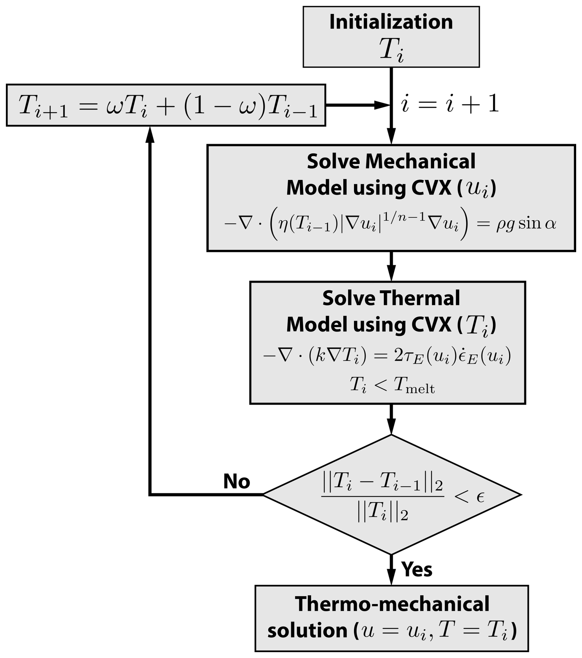
Figure 3Flowchart of our thermomechanical coupling scheme. We solve the mechanical and thermal free-boundary problems sequentially using CVX (Grant and Boyd, 2014) and couple them through an under-relaxed fixed-point iteration of temperature. The temperature indices are schematic: convergence is checked after the thermal solve, and the relaxed temperature is used in the next mechanical solve if needed. The thermal minimization enforces T≤Tmelt; the displayed diffusion equation applies where T<Tmelt. We iterate until the temperature residual falls below the prescribed tolerance, ε.
2.3 Verification
To verify the accuracy of our implementation of the mechanical model, we benchmark against the analytical solution derived for an idealized valley glacier in Schoof (2006b). This test case consists of a simplified glacier valley geometry underlain by saturated sediments, with variable pore pressure resulting from a specified elevation of the water table. Different failure regions become apparent when the elevation of the water table and the driving stress are varied. Figure 4a shows the model setup of a triangular computational domain, with the elevation of the water table denoted by a dashed line and the failure patches shown in red. In Fig. 4a, we reproduce Fig. 5 from Schoof (2006b) with the developed method by simulating the four distinct failure regimes. We demonstrate that our solver using a nominal grid spacing of Δx=0.02 reproduces the velocity field and failure patches of Schoof (2006b). The small deviations between our numerical solution and the benchmark arise from our finite discretization of the domain.
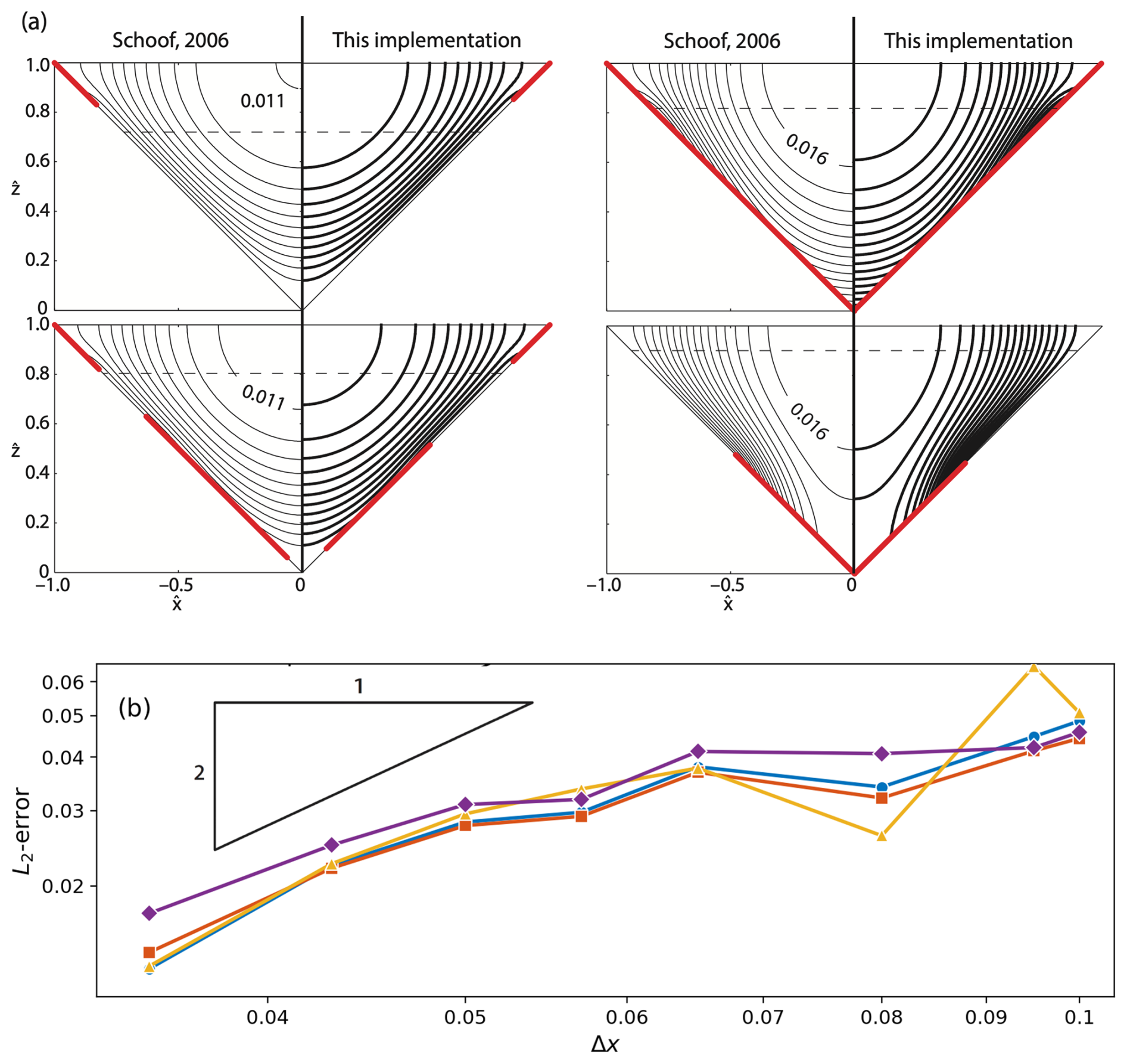
Figure 4Verification of our numerical implementation of the mechanical model against Schoof (2006b). (a) Contours of flow speed for an idealized valley glacier as specified in Schoof (2006b). Mimicking Fig. 5 in Schoof (2006b), the dashed line signifies the water table, with each flow regime chosen to exhibit markedly different regions of till failure (red lines). (b) Convergence plots of the normalized L2-error on surface velocities, computed against the most refined solution with the four curves representing the four benchmark examples shown in (a). We observe the expected second-order convergence of linear finite elements.
We perform a numerical convergence analysis of Ortholine for each of these benchmark solutions, shown in Fig. 4b. This is a self-convergence study: we compute the normalized L2-error of the surface velocities against our own most refined simulation as the grid is refined, which isolates the numerical discretization error and confirms that the solver converges at the expected rate. The error exhibits second-order convergence with grid refinement. The linear finite elements have polynomial degree p=1 and an expected p+1, or second-order, convergence rate in the L2 norm (Brenner and Scott, 2008). The observed second-order numerical convergence makes us confident that our implementation of the numerical method is correct and consistent. We are not aware of a verification case of a thermomechanically coupled free-boundary problem that would allow us to perform a similar analysis for thermally variable ice.
Ortholine is intended as a general framework that can in principle be applied to any field site, where the properties of the shear margins are of specific interest. However, the model has more potential to lead to valuable scientific insights at field sites where the shear margin is only partially controlled by topography, where subglacial conditions are thought to vary, and where field observations are available to constrain bed conditions. Figure 5 outlines the workflow for applying Ortholine to a given field site. We illustrate these steps below for the example of Institute Ice Stream located in the Ronne Ice Shelf region of West Antarctica.
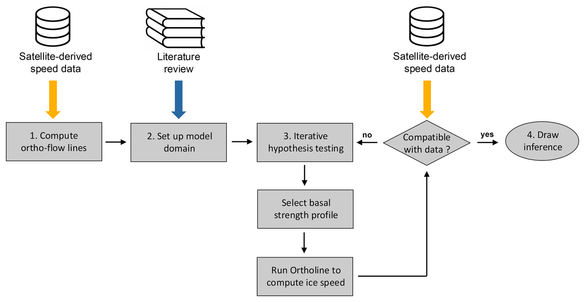
Figure 5Flowchart for the application of Ortholine to a given field site. Each of the four main steps is discussed in detail in Sect. 3. The only necessary data set for setting up the model is surface-velocity data (labeled “speed data” in the diagram), typically derived from satellite-based measurements. These data provide both direction and magnitude for computing ortho-flow lines. Other data can be valuable to integrate (blue arrow), but only surface-velocity data are necessary (orange arrow).
3.1 Compute ortho-flow lines
The classical conceptualization of ice streams by Raymond (1996) posits a plug-like motion in the trunk of the ice stream bordered by two narrow shear margins on the sides, yielding a flow configuration that is symmetric around the center line of the stream. In that limit, a simple linear transect that is orthogonal to the main flow direction and cuts through both shear margins is in a state of antiplane shear, as assumed in many idealized shear-margin models (Jacobson and Raymond, 1998; Suckale et al., 2014; Perol et al., 2015; Haseloff et al., 2015). Although there are examples of ice streams that fit this original conceptualization, such as Kamb Ice Stream (Elsworth and Suckale, 2016), the majority of field sites will not.
To analyze shear-margin properties in the field, the first step is to compute the curves that represent the closest equivalent to the simple cross-sectional transect envisioned by Raymond (1996). Because the antiplane approximation requires the model plane to be orthogonal to the local ice-flow direction (see Sect. 1), these curves are not in general straight transects but follow the local flow geometry. We refer to this set of curves as ortho-flow lines to highlight that their orientation is orthogonal to the local direction of ice velocity, For irrotational flow, these lines correspond to isocontours of the velocity potential, φ(∇φ=ud). We numerically generate ortho-flow lines from the velocity field derived from existing satellite data (Rignot et al., 2011). The velocity field need not satisfy the irrotationality condition : physical shear as well as observational noise can produce rotational flow. If the flow is not irrotational, we cannot directly solve for the velocity potential. Instead, we compute ortho-flow lines through numerical integration starting from a seed point in the center of the ice stream, x0. Velocity vectors are perpendicular to the ortho-flow line, which we generate from the stream center outward through Euler integration,
with step size, Δx. The resolution of the computation is smaller than the resolution of the observed velocity field, ud. This procedure generates an ortho-flow line, x, with a maximal antiplane velocity component and a near-zero in-plane velocity component. When the downstream ice speed drops below 10 m yr−1, this approach becomes noisy and we extend the ortho-flow line linearly.
Figure 6a shows a computed ortho-flow line cutting across the trunk of Institute Ice Stream as a gray line. We emphasize that this ortho-flow line is one of many possible ones. Our ortho-flow line is approximately linear near the center line of the stream, highlighting that Institute partially abides by the original conceptualization of ice streams by Raymond (1996). However, as the ortho-flow line approaches the margins of the ice stream, it increasingly curves to partially align with the main flow direction, particularly near the western shear margin where we intentionally extend it until ice speed drops below 10 m yr−1. The pronounced curvature of the ortho-flow line in the western shear margin is the consequence of lateral influx of ice through several smaller tributaries visible in Fig. 6a. It highlights that the ortho-flow line A–A' is dynamically coupled to stresses tens of kilometers further downstream through an extended marginal zone highlighted in Fig. 6c.
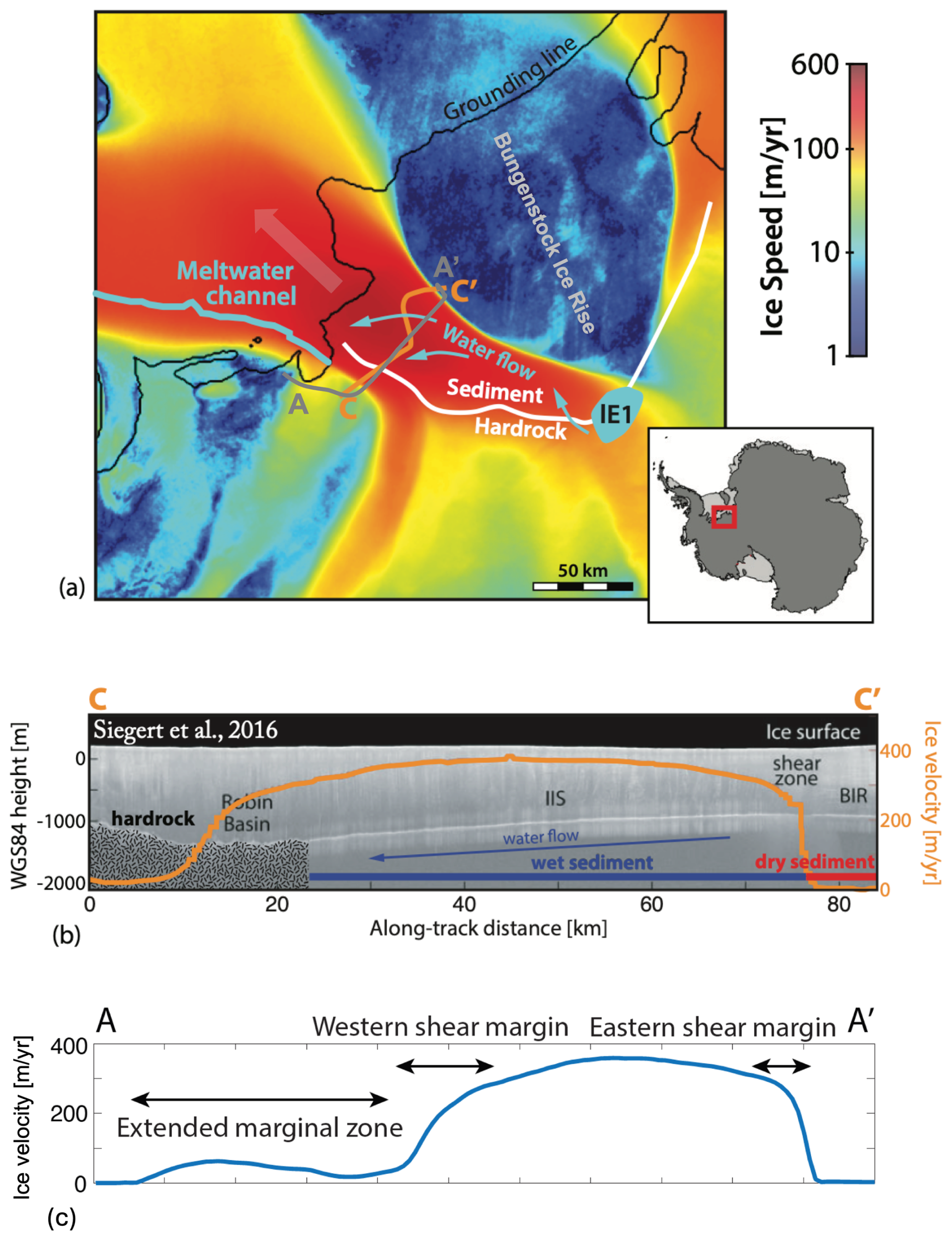
Figure 6Application of Ortholine to Institute Ice Stream. (a) Map of the ice speed in the study area derived from satellite radar data (Rignot et al., 2011) and generated with the Antarctic Mapping Toolbox (Greene et al., 2017). The flow direction is highlighted as a thick, transparent arrow. The shear margins are the distinct lateral transitions from fast (red) to slow flow (blue). The inferred rock-sediment transition from Siegert et al. (2016) is indicated as a white line. We denote the main features of the subglacial hydrology in blue, including the active subglacial lake E1 (Smith et al., 2009), hydropotential flow paths (Siegert et al., 2016), and a meltwater channel carved into the ice shelf (Le Brocq et al., 2013). Our ortho-flow line is indicated in gray and extends from A to A'. (b) Radar cross-section along C–C' from Siegert et al. (2016), showing basal topography and inferred subglacial conditions. We superimpose the downstream ice speed as an orange line. Inferred hydropotential gradients (Siegert et al., 2016) suggest that water flow propagates from the shear margin on top of sediment to the shear margin on hard rock. We choose to focus on the ortho-flow line A–A' because of its proximity to the radar cross-section C–C' from Siegert et al. (2016). (c) Observed surface-speed profile along A–A', showing the extended marginal zone and the western and eastern shear margins.
3.2 Set up the model domain
To set up the Ortholine model domain, we chose the ortho-flow line A–A'. In principle, Ortholine could represent any ortho-flow line, but some ortho-flow lines might be more suitable than others. For example, it might not be ideal to select an ortho-flow line that crosses the grounding line, because grounding-line processes are not currently included in the model. Also, it can be valuable to select an ortho-flow line where data from previous field campaigns can shed additional light on basal processes. While only a surface-velocity data set is strictly necessary for setting up Ortholine, other constraints could elevate the scientific contribution of the modeling. We illustrate this process through a short literature review for Institute Ice Stream.
At Institute, streaming ice is bounded to the east by Bungenstock Ice Rise, and fed from the west by tributaries from the Ellsworth Mountains (Ross et al., 2011, 2014). As evident from the ice-speed map in Fig. 6a, the eastern shear margin near the Bungenstock Ice Rise is very sharp, but the western shear margin is much less localized (Scambos et al., 2004). This asymmetry on the surface is mirrored by different subglacial conditions at the base of the ice, with the eastern shear margin underlain by sediments and the western shear margin underlain by a hard-rock bed, as inferred from the radar profile C–C' shown in Fig. 6b (Siegert et al., 2016). The basal topography across this profile is relatively subdued, making it unlikely that topographic control is the primary factor determining the shear margin position.
In the 2010–2011 field season, the British Antarctic Survey completed extensive airborne geophysical surveys of the area, including radar sounding, gravity, magnetics, and LIDAR (Jordan et al., 2013). These geophysical data constrain the various factors that contribute to the dynamics of Institute Ice Stream, including topography, lithology, and hydrology. Siegert et al. (2016) highlight subglacial hydrology as an important factor that could induce rapid rearrangement in Institute's trunk. The trunk is downstream of an active subglacial lake, Institute E1 (Smith et al., 2009) highlighted in Fig. 6a, and meltwater emanates from the western shear margin at the grounding line (Le Brocq et al., 2013; Alley et al., 2016) in the form of a channel. The hydraulic potential of Institute Ice Stream suggests that subglacial meltwater is routed from the eastern shear margin to the western shear margin (Siegert et al., 2016). The white line in Fig. 6a represents a transition between subglacial sediments and hard rock, as inferred by Siegert et al. (2016) from radar sounding data.
For the remainder of this section, we choose to focus on ortho-flow line A–A', because of its proximity to the radar profile C–C' (Siegert et al., 2016). At this location, the main ice stream trunk is approximately 60 km wide, with a maximum ice thickness of about 1700 m near the western margin. We simplify the geometry of the actual bed profile by assuming a model domain with a flat surface and a bed that is piecewise-linear, neglecting roughness. For the characteristic driving stress of the region we use a representative ice thickness, H=1275 m, giving , with ice density, ρ=917 kg m−3, acceleration due to gravity, g=9.8 m s−2, and surface slope, α=0.0024. The full thickness variation across the trunk (from approximately 1000 m near the eastern to about 1700 m near the western margin) enters the overburden-dependent bed strength through Eq. (31).
Based on the interpretation of radio-echo sounding data, Siegert et al. (2016) suggest that the lithology underneath Institute transitions from sediment to hard rock in the across-flow direction (see Fig. 6b). Both the bed roughness and the return power of the radio-echo sound provide evidence in favor of this interpretation (Siegert et al., 2016). We separate the bed into two boundary conditions specified by regions identified by Siegert et al. (2016) as hard rock and saturated sediments, respectively. Within the sediment-occupied zone, we impose a sharp increase in the prescribed till strength τc outside of the eastern shear margin to represent a transition from temperate to frozen conditions, as inferred by Siegert et al. (2016). Rather than raising the total strength τc directly, one could equivalently adjust individual parameters such as the cohesion c where independent information exists for how they change under frozen conditions.
The trunk of Institute Ice Stream (see Fig. 6a) is underlain by a complex subglacial drainage system involving a lake upstream (Smith et al., 2009), lateral meltwater drainage in the main trunk, and a meltwater channel emanating from the grounding line in the vicinity of the western shear margin (Le Brocq et al., 2013). We assume that distributed drainage can be approximated as a thin film of meltwater and that efficient drainage occurs through a Röthlisberger channel (Röthlisberger, 1972) operating at low pore pressure (Hewitt, 2011; Perol et al., 2015; Elsworth and Suckale, 2016). The reduction in pore pressure in the vicinity of the channel depends on the channel discharge and the decay length of the pressure perturbation scales with the film thickness of the distributed system, as derived in more detail in Perol et al. (2015).
We model the decline of bed strength away from a subglacial drainage channel located at Y using a localized pore-pressure deficit, , where p∞ is the background pore pressure, Δp>0 is the pressure reduction at the channel, and γ is its decay length.
similar to a previous study of the effect of channelized drainage on shear margins (Elsworth and Suckale, 2016). The exponential form follows the treatment of Perol et al. (2015): the pore-pressure reduction near a channel reflects the competition between drainage into the channel and resupply from the surrounding distributed system, which to leading order yields a perturbation that decays exponentially away from the channel, with a decay length set by the film thickness of the distributed system.
Another factor modifying subglacial drainage in our domain is the variable overburden of the ice. The approximately linear basal topography across the trunk implies that ice thickness increases from approximately 1000 m near the eastern to about 1700 m near the western margin. We capture the effect of overburden pressure on the underlying hydrological system by making the basal strength, τc, a function of the effective pressure at the bed:
To link the pore pressure to the overburden, we take the pore pressure to be a fixed fraction of the overburden, p(y)=kp ρgH(y), which corresponds to a spatially near-constant flotation fraction across the trunk. Substituting this relation gives
with friction parameter, (Rathbun et al., 2008), sediment cohesion, c≈1–2 kPa (Kamb, 2001), and flotation fraction, kp, which varies from 0 (no flotation) to 1 (full flotation). We do not treat kp as an independent free parameter in the convex solve for lack of constraints on how it might vary. Instead, we prescribe a basal-strength profile that varies linearly with ice thickness H and adjust the corresponding strength coefficients so that the modeled surface speed and transverse strain rate best match the MEaSUREs observations along the ortho-flow line.
3.3 Iterative hypothesis testing
The central idea of iterative hypothesis testing with Ortholine is that different basal processes generate distinct spatial profiles of basal strength, but only some of these profiles are consistent with observed surface velocities. Similarly, different basal processes have distinct implications for the subglacial melt rate that could be evaluated against observations of basal hydrology. For example, subglacial drainage can occur in multiple configurations (e.g., Flowers, 2015), each implying a different basal-strength profile. A channelized system would produce localized strengthening that decays away from the channel (Perol et al., 2015), whereas a distributed thin film would yield a more uniform bed strength. By testing which basal strength profiles reproduce measured surface speeds, Ortholine constrains which basal processes are plausible at a given field site. Also, the hypothesized hydrological drainage elements need to be fed by melting of ice and can hence be evaluated for consistency with ice dynamics.
In Fig. 7, we illustrate how to test the hypothesis that basal strength underneath the fast-moving portion of Institute Ice Stream is dominated by ice overburden. We compare two simulations, one in which we assume that ice overburden does not affect the basal strength (panels a1–a5) and one in which ice overburden is the primary control (panels b1–b5). More specifically, we assume that the bed strength is constant for the simulation on the left, as would be the case if variable ice thickness did not matter. For the simulations on the right, we assume that pore pressure increases with ice overburden (see Eq. 31), leading to a bed strength that varies linearly with ice thickness H and is maximal at the topographic low. In both cases, we only show the simulation that best reproduces the observed surface speed.
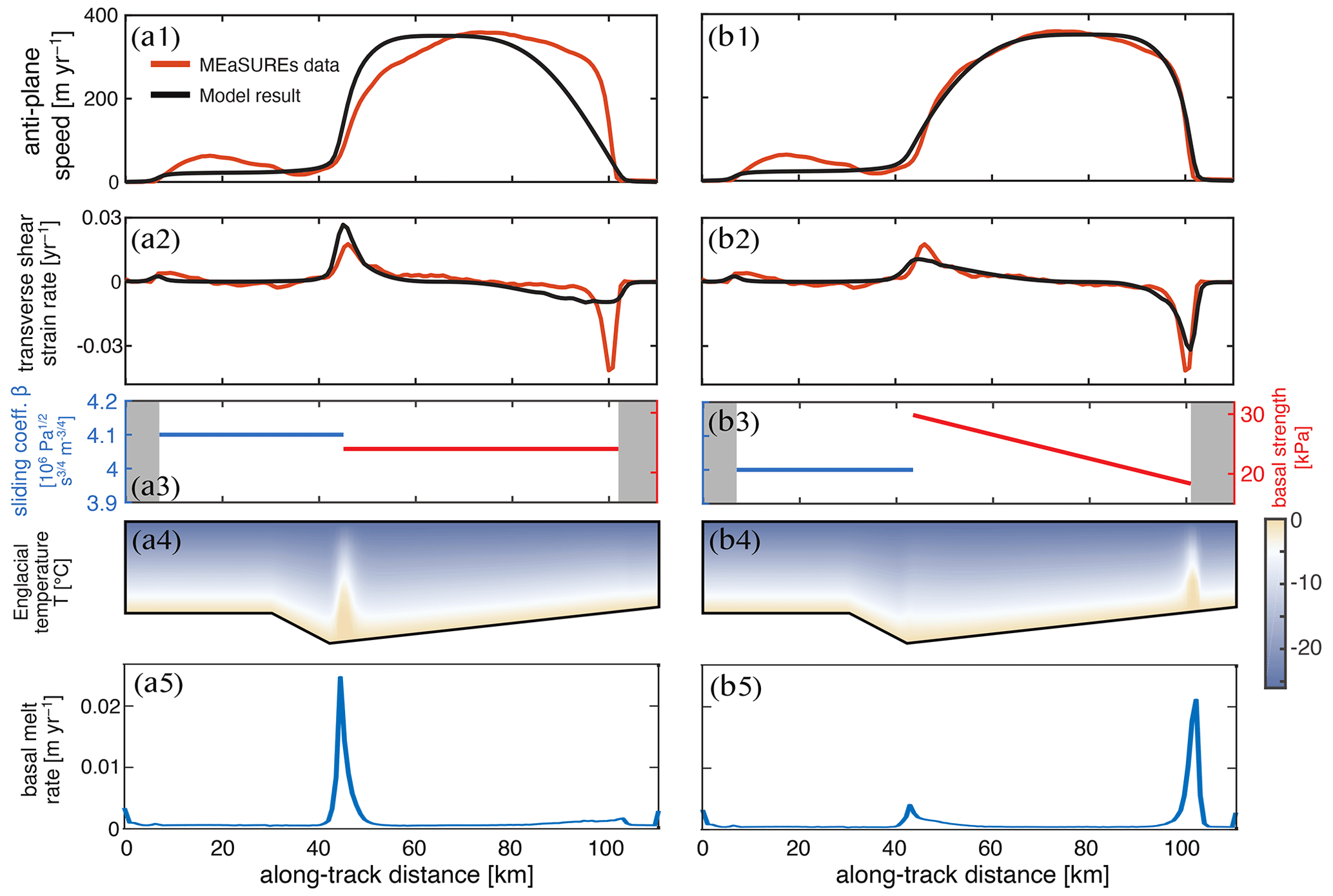
Figure 7Numerical experiment investigating the relative importance of ice overburden. (a) Counterfactual simulation assuming uniform basal strength in the sediment indicative of ice overburden not being important. (b) Simulation assuming linearly increasing basal strength in the sediment as a function of overburden pressure. Rows illustrate: (1) Comparison of modeled velocities to observed MEaSUREs surface velocities across profile A–A'. (2) The modeled and observed transverse shear strain-rate component, , across A–A' (yr−1). (3) Tuned basal conditions, with locations specified from observations. Hard-rock sliding parameter (blue), saturated sediment strength (red), and locked sediments (gray). (4) Englacial temperature field within the ice column. (5) Melt rate at the base of the ice.
For both simulations, the rows in Fig. 7 show the calculated downstream speed compared to the observed surface speed (panels a1 and b1), the calculated and observed transverse strain rates (panels a2 and b2), the hard-rock sliding parameter and sediment strength of the best-fitting computation (panels a3 and b3), the englacial temperature distribution (panels a4 and b4) and the resulting subglacial melt rate (panels a5 and b5). In both cases, we assume that the lithologic transition from rock (blue line in a3 and b3) to sediment (red line in a3 and b3) occurs in the vicinity of the western shear margin and that the ice trunk is bordered by areas of frozen basal conditions (shown in gray). In general, the computation based on the linear decrease in sediment strength from the western to the eastern shear margin fits observed surface speed much better (Fig. 7b1 vs a1). The best-fit strength profile varies linearly from 29.85 to 18.35 kPa across the ice stream trunk, mimicking the approximately linear basal topography across the trunk for an approximately constant average flotation factor of kp=0.996. We note that this flotation fraction is diagnosed from this best-fit strength profile, together with representative values of the friction coefficient Cf and sediment cohesion c, and would vary if other values for Cf and c were chosen.
An interesting nuance of the analysis is that the ice overburden not only affects the basal strength, but also exhibits an indirect control on the englacial temperature and on subglacial melt rate. The reason is that for the computation on the left (panels a1–a4), the sediment portion of the bed is relatively weak and the hard-rock portion of the bed plays a more important role in the overall force balance. In contrast, sediment strength increases significantly from the eastern to the western shear margin for the computation on the right (panels b1–b4). The high basal strength in parts of the sediment portion means that the sliding coefficient of the rock portion of the bed is relatively lower, reducing shear heating near the western shear margin (see Fig. 7b4) compared to the case where the sliding coefficient is high in both segments (see Fig. 7a4). As a consequence, meltwater is generated in different locations with melt concentrated near the topographic low in Fig. 7a5 as opposed to near the eastern shear margin in Fig. 7b5.
Although Fig. 7b1 fits the measured ice speed well for most of the ice-stream trunk, it reproduces the surface speed in the extended marginal zone less well. This disconnect suggests that a physical process other than ice overburden controls the basal strength distribution in the extended marginal zone. A likely candidate is subglacial hydrology, because the meltwater channel that emanates from below the western shear margin at the grounding line (see Fig. 6a) likely extends upstream into the trough near the western shear margin. The meltwater channel locally strengthens the bed (see Eq. 29), but little is known about how quickly the pressure perturbation induced by a meltwater channel decays spatially in the presence of both lithological and topographic variations. For a plastic bed, we assume a constant decay length, γ, everywhere, implying that the channel alters the bed strength similarly irrespective of the lithology and local topography.
The existence of a meltwater channel near the western shear margin is well supported by observational data (e.g., see Fig. 6 and accompanying text). Less clear is how this meltwater channel affects basal strength. In Fig. 8, we test the hypothesis that a channel leads to an exponential increase in basal strength near the western shear margin. We compare two simulations: one represents velocity-strengthening sliding over hard rock (Fig. 8a1–a5), and the other assumes Coulomb sliding (Fig. 8b1–b5). In the sediment-dominated portion of the domain, we superimpose the basal strengthening of the channel with a linear decrease in bed strength towards the eastern shear margin as a result of decreasing overburden (see Fig. 7). The agreement between modeled and observed surface speeds (Fig. 8a1, b1) and strain rates (Fig. 8a2, b2) in the extended marginal zone improves significantly compared to Fig. 7 The quality of fit is comparable for both simulations, highlighting that both basal-strength distributions have comparable explanatory potential.
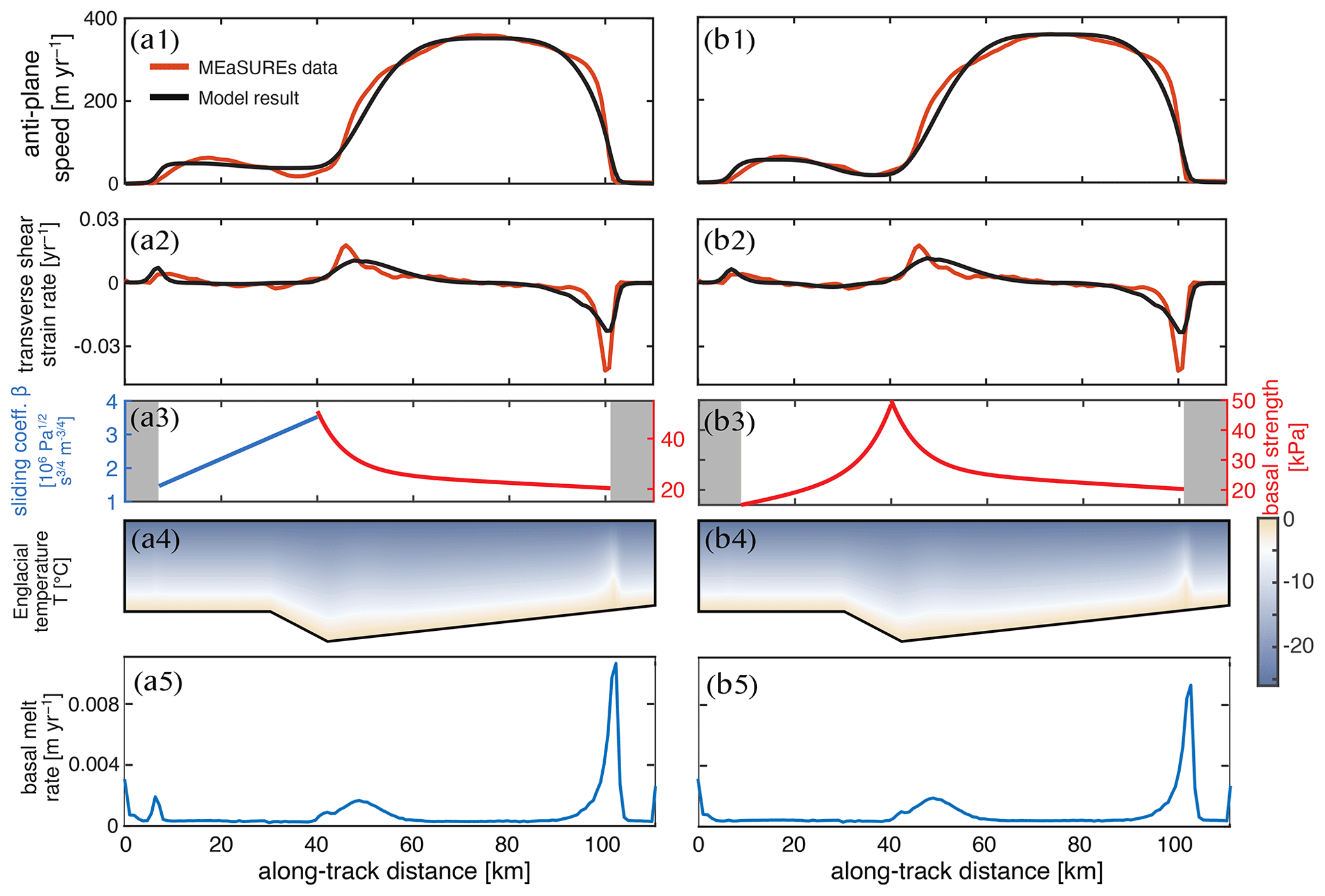
Figure 8Numerical experiment to assess the relative importance of a channel located in the trough near the western shear margin. (a) Simulation assuming velocity-strengthening sliding over hard rock. (b) Simulation assuming Coulomb sliding in the extended marginal zone. Both simulations include channel-related strengthening near the western shear margin. Rows illustrate: (1) Comparison of modeled velocities to observed MEaSUREs surface velocities across profile A–A′. (2) The modeled and observed transverse shear strain-rate component, , across A–A' (yr−1). (3) Tuned basal conditions, showing the hard-rock sliding parameter in blue and plastic-bed strength in red. (4) Temperature field in the ice column. (5) Melt rate at the base of the ice.
To create a counterfactual for Fig. 8 that represents a scenario without a meltwater channel in the trough below the western shear margin, we assume that the presence of pervasive subglacial water leads to regularized Coulomb sliding in the hard-rock portion of our model domain (Lliboutry, 1968; Iken, 1981; Fowler, 1986, 1987; Schoof, 2005; Gagliardini et al., 2007). In Fig. 9, we test whether a plastic bed with variable strength improves the fit to observed surface speeds in the western shear margin and extended marginal zone. Similarly to Fig. 7, we restrict our tests to constant and linearly varying basal strength profiles. To highlight that regularized Coulomb sliding is equivalent to plastic behavior of the bed, we plot both the hard-rock and the sediment-dominated portion of the domain in red in Fig. 9a3 and b3. Building on our analysis from Fig. 7, we assume that the basal strength of the sediments decreases linearly from the western to the eastern shear margin.
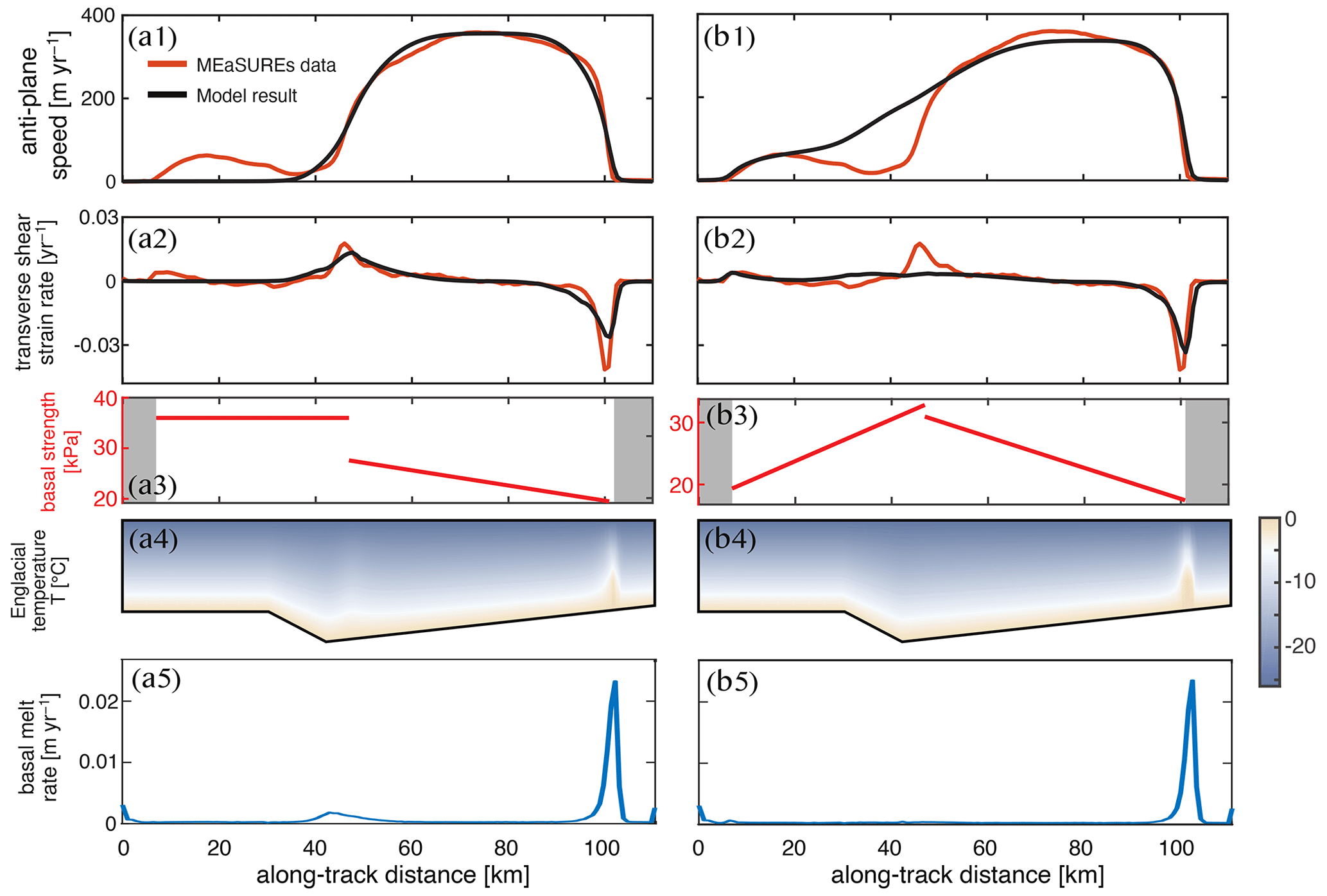
Figure 9Counterfactual simulations assuming the absence of a meltwater channel near the western shear margin. (a) Simulation assuming that regularized Coulomb sliding over hard rock leads to approximately uniform basal strength. (b) Simulation assuming regularized Coulomb sliding with a linearly increasing basal strength in the extended marginal zone. Rows illustrate: (1) Comparison of modeled velocities to observed MEaSUREs surface velocities across profile A–A'. (2) The modeled and observed transverse shear strain-rate component, , across A–A' (yr−1). (3) Basal strength of the plastically behaving bed. (4) Temperature field in the ice column. (5) Melt rate at the base of the ice.
The two best fitting simulations shown in Fig. 9 demonstrate that switching the nature of sliding does not improve the fit to observed surface speed and strain rates. When assuming a constant basal strength, we are unable to reproduce the slow but finite sliding outside of the western shear margin (see Fig. 9a1). In comparison, velocity-strengthening sliding (see Fig. 7) is consistent with the observed slow slip. A linearly increasing basal strength profile provides a better fit in the extended marginal zone, but fails to capture the western shear margin (see Fig. 9b1 and b2). We emphasize that, contrary to Fig. 7, it is also not clear why the basal strength in the extended marginal zone would increase linearly, because ice overburden does not vary much in the extended marginal zone.
3.4 Drawing inferences about the physical processes controlling shear-margin position and stability
Figure 7 suggests that the simplest hydrological system capable of reproducing the observed surface speed at Institute Ice Stream is a spatially well-connected drainage network near flotation. The simplest physical process that could explain the properties of this drainage network is variable ice overburden on a temperate bed with variable basal topography. Needless to say, there is almost certainly considerable small-scale variability not captured in Ortholine. However, this small-scale variability might not affect surface speed because ice acts as a low-pass filter on basal topography and slipperiness, as analyzed in more detail in Gudmundsson (2003).
Transfer functions, pioneered by Gudmundsson (2003), are an approach to estimating the wavelength below which small-scale variability in basal topography or slipperiness is likely not relevant for surface velocities unless this small-scale variability is coupled with other basal processes. For example, a small topographic low containing a meltwater channel can still be dynamically relevant, not because of its own spatial scale but because of its large-scale effects on water routing. For example, the best fitting simulation shown in Fig. 7b1–b4 entails a temperate zone in the eastern shear margin that could feed a meltwater channel causing local strengthening of the bed (Perol and Rice, 2015; Platt et al., 2016; Suckale et al., 2014; Elsworth and Suckale, 2016). Alternatively, the increase in bed strength could result from freezing (Schoof, 2004, 2012; Suckale et al., 2014; Perol et al., 2015; Haseloff et al., 2015). The latter explanation would require lateral advection of cold ice into the eastern shear margin to counteract the heating entailed in the measured strain rates (Fig. 7b2) and an additional englacial process like fabric to explain the narrow margin width.
Further evidence for the importance of small-scale variability in subglacial hydrology comes from Fig. 8, which suggests that the basal strength distribution over the hard-rock bed is dominated by the existence of a meltwater channel in or close to the western shear margin. However, Fig. 7 demonstrates that the presence of this channel is not a necessary component to obtain a satisfactory fit to the surface speed and strain rates in most of the domain. This finding suggests that the channel is an important physical control for the western but not necessarily for the eastern shear margin. Given the pronounced lateral asymmetries in topography, lithology, and subglacial hydrology at Institute (see Sect. 3.2) it is perhaps not surprising that the two shear margins could be controlled by different physical processes.
When drawing inferences about the physical processes controlling shear-margin properties through Ortholine, it is important to keep in mind that individual factors, such as topography, lithology, temperature, and subglacial hydrology, can be interconnected. This interconnectivity is the reason why it is challenging to derive insights into the physical processes controlling shear-margin properties from observational data alone, particularly for field sites like Institute where all of these factors vary simultaneously. Similarly, there may be large-scale variations that correlate with or follow a trend similar to overburden stress and are therefore difficult to differentiate from effects of ice thickness. We merely note here that it is not necessary to invoke this complexity in most of the domain for the model to be compatible with surface observables (Fig. 7b1).
To disentangle the various dependencies, Ortholine uses simple auxiliary assumptions (e.g., Eqs. 29 and 31) to link spatial variability in subglacial hydrology to specific physical processes such as ice overburden or the presence of a Röthlisberger channel. These auxiliary assumptions can be adjusted by the user. Generally, we recommend keeping the number of free parameters used in these auxiliary assumptions small to reduce the risk of overfitting. A similar strategy was recently used in Summers et al. (2023) to constrain the physical processes controlling shear-margin behavior at Thwaites, albeit in the context of a different modeling approach. We have deliberately framed this step as forward hypothesis testing rather than as a formal inversion of the basal strength from the surface velocities. The choices that enter the auxiliary assumptions are unavoidable in either framing, but making them explicit and physically motivated, rather than folding them into the regularization and priors of an inversion, keeps the small number of free parameters transparent. The two approaches are complementary: an inversion could propose a basal-strength profile and the forward model could then test which physical processes are capable of producing it, and the balance between the two is ultimately for the user to decide.
Ortholine is designed to evaluate the relative importance of different englacial and subglacial processes in controlling a specific shear-margin position. The main value of this insight for making inferences about future shear-margin stability lies in realizing that different physical processes evolve on different time scales. Topographically controlled shear margins are the most stable, the shear margin at Lambert Glacier being one example (Sanderson et al., 2023). Thermal processes such as thawing of the subglacial bed can lead to shear-margin migration (Schoof, 2012) that is much faster than topographic change or erosion, but still comparatively slower than hydrological processes that can lead to sudden rearrangements of shear-margin position (Alley et al., 1994; Catania et al., 2006; Elsworth and Suckale, 2016).
Different models have different strengths and weaknesses. Ice-sheet models such as the Ice Sheet System Model (Larour et al., 2012) or the Parallel Ice Sheet Model (Bueler and Brown, 2009) aim for realism by capturing the full two- or three-dimensional stress balance. They can represent lateral drag, tributary inflow, and grounding line migration in complex geometries, but these advantages come at the cost of high computational demand and significant data requirements to constrain all model parameters (Kirchner et al., 2011). Flow-line models, by contrast, neglect lateral drag and assume simplified geometries, but are computationally efficient (Nye, 1952). They are tools for hypothesis testing by isolating a particular aspect of ice dynamics and focusing on analyzing its impact and have advanced our understanding of how longitudinal stress gradients change the transient responses of glaciers to external forcing (Pattyn, 2002) or how grounding-line stability varies with basal drag and rheology (Schoof, 2007).
Conceptually, Ortholine follows the modeling philosophy of flow-line models, in which some aspects of ice dynamics are intentionally simplified or neglected to isolate the effect of others, and is complementary to them: instead of focusing on the longitudinal stress balance along a flow line while neglecting lateral effects, Ortholine focuses on lateral stresses while neglecting longitudinal effects.
Currently, evaluations of shear-margin stability are typically based on a qualitative comparison of whether the shear-margin coincides with distinctive topographic features or not (e.g., MacGregor et al., 2013; Sanderson et al., 2023). For example, MacGregor et al. (2013) argued that the eastern shear margin at Thwaites Glacier could be prone to migration because the topography below the eastern shear margin is flat. However, a more in-depth quantitative analysis of the shear margins at Thwaites (Summers et al., 2023) shows that this criterion alone is not sufficient to assess shear-margin stability. Many other processes affect shear-margin dynamics sensitively, from basal processes such as subglacial hydrology to regional-scale mass balance leading to rapid ice thinning at Thwaites (Smith et al., 2020).
Similarly, the presence of pronounced topography does not necessarily imply margin stability. For example, Summers et al. (2023) show that the western shear margin at Thwaites Glacier could also be prone to migration despite being located in an area of much more pronounced topography. Our simulations for Institute support this more nuanced view of shear-margin controls: despite the western shear margin at Institute being approximately co-located with a topographic trough, our simulations suggest that the presence of a meltwater channel in this trough is important, as evidenced by simulations with a meltwater channel (see Fig. 8a1 and b1) fitting observed surface speeds much better than simulations without a channel (see Fig. 9a1 and b1).
In addition to the inspiration we take from flow-line models, our model is motivated by the insights of previous antiplane shear models of shear margins (Jacobson and Raymond, 1998; Schoof, 2004; Suckale et al., 2014; Perol and Rice, 2015; Haseloff et al., 2015; Elsworth and Suckale, 2016). At first, it might seem counterintuitive to adapt these highly idealized models to a particular field site, but this step is warranted by our advancing scientific understanding. We now have both observational (Harrison et al., 1998; Bindschadler and Vornberger, 1998; Echelmeyer and Harrison, 1999; Clarke et al., 2000; Catania et al., 2006) and theoretical evidence (Jacobson and Raymond, 1998; Schoof, 2004; Suckale et al., 2014; Perol and Rice, 2015; Haseloff et al., 2015; Elsworth and Suckale, 2016) that shear-margin migration is possible, in principle. The challenge now becomes to assess if and where shear-margin migration might occur not only in principle, but also in reality. This challenge is probably most acute for Thwaites Glacier (MacGregor et al., 2013; Summers et al., 2023), but also relevant for other regions, such as Institute, where accelerated melting at the grounding line is expected later this century (Hellmer et al., 2012).
In addition to our growing scientific understanding, the design of field-site-specific shear-margin models through Ortholine is enabled by the substantial increase in the resolution of remotely detected data probing the ice sheets (Schroeder et al., 2014; Siegert et al., 2016; Muto et al., 2019; Koellner et al., 2019). Radio-echo sounding (Schroeder et al., 2014; Siegert et al., 2016) and seismic (Muto et al., 2019; Koellner et al., 2019) surveys have advanced our ability to map heterogeneities in subglacial conditions. These increasingly detailed observations highlight that heterogeneity in basal conditions is the norm rather than the exception. The observed diversity is not surprising in light of the numerous physical processes at play in a heterogeneous subglacial environment (Schroeder et al., 2014; Siegert et al., 2016; Muto et al., 2019; Koellner et al., 2019). Increasingly, these detailed observations provide an important opportunity for models to better constrain the relative importance of the various physical processes that contribute to the dynamics of ice streams and their shear margins.
In this paper, we develop Ortholine, a thermomechanical, antiplane shear model. Ortholine is designed to evaluate the relative importance of englacial and subglacial processes controlling shear-margin location. Building on the variational formulation by Schoof (2006b), we frame the problem in more flexible Disciplined Convex Programming (Grant et al., 2006) and implement a numerical solution using the software package CVX (Grant and Boyd, 2014). We verify our numerical implementation against the idealized mountain glacier case proposed by Schoof (2006b). We then illustrate the four key steps for applying the model to a given field site, using Institute Ice Stream as a proof-of-concept. Our simulations show that identifying the physical processes governing shear-margin stability through spatial association alone is not reliable. The presence of a topographic trough below a shear margin does not necessarily imply that the position of this shear margin is topographically controlled, as highlighted by the example of the western shear margin at Institute. Similarly, the presence of a gently sloping topography does not mean that topographic effects are irrelevant, as demonstrated in Fig. 7. Ortholine provides a framework for evaluating the relative importance of different physical processes across an antiplane cross-section in a transparent, if simplified, way.
Observational data including MEaSUREs surface velocity measurements and locations of subglacially sourced channels are publicly available through the National Snow & Ice Data Center (https://nsidc.org/data/, last access: 21 September 2026). The code developed in this paper is open source (https://github.com/coopere/InstituteIceStream2D, last access: 21 September 2026) under the GNU General Public License, version 3 (GPL-3.0). The specific version of the code used to create the results in this manuscript is ortholine_v1.1 (Elsworth, 2026), archived at https://doi.org/10.5281/zenodo.20858511.
JS supervised the different stages of the study, participated in the conceptualization of the model, wrote the manuscript, and provided funding for all authors involved. CE led the early model and numerical method development stages, implemented the CVX-based version of the code, performed the verification analysis, and wrote the Methods section of the manuscript. NA performed the reproduction analysis and helped improve the code. All authors have reviewed and approved the final version of the manuscript.
The contact author has declared that none of the authors has any competing interests.
Publisher's note: Copernicus Publications remains neutral with regard to jurisdictional claims made in the text, published maps, institutional affiliations, or any other geographical representation in this paper. The authors bear the ultimate responsibility for providing appropriate place names. Views expressed in the text are those of the authors and do not necessarily reflect the views of the publisher.
This work benefited greatly from the input of Paul Summers, Anuj Shetty, and Samantha Hordyk. The authors thank Dustin Schroeder, Neal Iverson, Lucas Zoet, Knut Christianson, and Mark Fahnestock for fruitful discussions.
This research has been supported by the National Science Foundation, Directorate for Geosciences, Office of Polar Programs (grant nos. 1341499, 1744758, and 1739027).
This paper was edited by Ludovic Räss and reviewed by two anonymous referees.
Alley, K. E., Scambos, T. A., Siegfried, M. R., and Fricker, H. A.: Impacts of warm water on Antarctic ice shelf stability through basal channel formation, Nat. Geosci., 9, 290–293, https://doi.org/10.1038/ngeo2675, 2016. a
Alley, K. E., Scambos, T. A., Anderson, R. S., Rajaram, H., Pope, A., and Haran, T. M.: Continent-wide estimates of Antarctic strain rates from Landsat 8-derived velocity grids, J. Glaciol., 64, 321–332, https://doi.org/10.1017/jog.2018.23, 2018. a, b
Alley, R. B., Anandakrishnan, S., Bentley, C. R., and Lord, N.: A water-piracy hypothesis for the stagnation of Ice Stream C, Antarctica, Ann. Glaciol., 20, 187–194, https://doi.org/10.3189/172756494794587032, 1994. a
Bamber, J. L., Vaughan, D. G., and Joughin, I.: Widespread complex flow in the interior of the Antarctic ice sheet, Science, 287, 1248–1250, https://doi.org/10.1126/science.287.5456.1248, 2000. a
Bindschadler, R. and Vornberger, P. L.: Changes in the West Antarctic Ice Sheet Since 1963 from Declassified Satellite Photography, Science, 279, 689–692, https://doi.org/10.1126/science.279.5351.689, 1998. a, b
Bingham, R. G. and Siegert, M. J.: Radar-derived bed roughness characterization of Institute and Möller ice streams, West Antarctica, and comparison with Siple Coast ice streams, Geophys. Res. Lett., 34, L21504, https://doi.org/10.1029/2007GL031483, 2007. a, b
Brenner, S. C. and Scott, L. R.: The Mathematical Theory of Finite Element Methods, 3rd edn., Texts in Applied Mathematics, vol. 15, Springer, https://doi.org/10.1007/978-0-387-75934-0, 2008. a
Bueler, E. and Brown, J.: Shallow shelf approximation as a “sliding law” in a thermomechanically coupled ice sheet model, J. Geophys. Res.-Earth, 114, F03008, https://doi.org/10.1029/2008JF001179, 2009. a
Catania, G. A., Scambos, T. A., Conway, H., and Raymond, C. F.: Sequential stagnation of Kamb Ice Stream, West Antarctica, Geophys. Res. Lett., 33, L14502, https://doi.org/10.1029/2006GL026430, 2006. a, b, c
Clarke, T. S., Liu, C., Lord, N. E., and Bentley, C. R.: Evidence for a recently abandoned shear margin adjacent to ice stream B2, Antarctica, from ice-penetrating radar measurements, J. Geophys. Res.: Solid Earth, 105, 13409–13422, https://doi.org/10.1029/2000JB900037, 2000. a, b
Echelmeyer, K. and Harrison, W.: Ongoing margin migration of ice stream B, Antarctica, J. Glaciol., 45, 361–369, https://doi.org/10.3189/002214399793377059, 1999. a, b
Elsworth, C. W.: coopere/InstituteIceStream2D: ortholine_v1.1, Zenodo [code], https://doi.org/10.5281/zenodo.20858511, 2026. a
Elsworth, C. W. and Suckale, J.: Rapid ice flow rearrangement induced by subglacial drainage in West Antarctica, Geophys. Res. Lett., 43, 11697–11707, https://doi.org/10.1002/2016GL070430, 2016. a, b, c, d, e, f, g, h, i, j, k
Flowers, G. E.: Modelling water flow under glaciers and ice sheets, P. Roy. Soc. A-Math. Phy., 471, 20140907, https://doi.org/10.1098/rspa.2014.0907, 2015. a
Fowler, A.: A sliding law for glaciers of constant viscosity in the presence of subglacial cavitation, Proc. R. Soc. Lond. Ser A Math. Phys. Sci., 407, 147–170, https://doi.org/10.1098/rspa.1986.0090, 1986. a
Fowler, A.: Sliding with cavity formation, J. Glaciol., 33, 255–267, https://doi.org/10.3189/S0022143000008820, 1987. a
Friedman, A.: Variational principles and free-boundary problems, Dover Publications, Mineola, NY, ISBN 978-0-486-47853-1, 2010. a
Gagliardini, O., Cohen, D., Råback, P., and Zwinger, T.: Finite-element modeling of subglacial cavities and related friction law, J. Geophys. Res.-Earth, 112, F02027, https://doi.org/10.1029/2006JF000576, 2007. a
Geuzaine, C. and Remacle, J.-F.: Gmsh: A three-dimensional finite element mesh generator with built-in pre- and post-processing facilities, Int. J. Numer. Methods Eng., 79, 1309–1331, https://doi.org/10.1002/nme.2579, 2009. a
Glen, J. W.: The creep of polycrystalline ice, Proc. R. Soc. Lond. Ser. A Math Phys. Sci., 228, 519–538, https://doi.org/10.1098/rspa.1955.0066, 1955. a
Grant, M. and Boyd, S.: CVX: Matlab Software for Disciplined Convex Programming, version 2.1, CVX Research [code], https://cvxr.com/cvx/ (last access: 5 January 2026), 2014. a, b, c, d, e, f
Grant, M., Boyd, S., and Ye, Y.: Disciplined Convex Programming, in: Global Optimization: From Theory to Implementation, edited by Liberti, L. and Maculan, N., 155–210, Springer, Boston, MA, https://doi.org/10.1007/0-387-30065-1_7, 2006. a, b
Greene, C. A., Gwyther, D. E., and Blankenship, D. D.: Antarctic Mapping Tools for MATLAB, Comp. Geosci., 104, 151–157, https://doi.org/10.1016/j.cageo.2016.08.003, 2017. a
Gudmundsson, G. H.: Transmission of basal variability to a glacier surface, J. Geophys. Res.: Solid Earth, 108, 2253, https://doi.org/10.1029/2002JB002107, 2003. a, b
Harrison, W., Echelmeyer, K., and Larsen, C.: Measurement of temperature in a margin of Ice Stream B, Antarctica: implications for margin migration and lateral drag, J. Glaciol., 44, 615–624, https://doi.org/10.3189/S0022143000002112, 1998. a, b
Haseloff, M., Schoof, C., and Gagliardini, O.: A boundary layer model for ice stream margins, J. Fluid Mech., 781, 353–387, https://doi.org/10.1017/jfm.2015.503, 2015. a, b, c, d, e, f, g
Haseloff, M., Hewitt, I., and Katz, R.: Englacial pore water localizes shear in temperate ice stream margins, J. Geophys. Res.-Earth, 124, 2521–2541, https://doi.org/10.1029/2019JF005399, 2019. a
Hellmer, H. H., Kauker, F., Timmermann, R., Determann, J., and Rae, J.: Twenty-first-century warming of a large Antarctic ice-shelf cavity by a redirected coastal current, Nature, 485, 225–228, https://doi.org/10.1038/nature11064, 2012. a
Hewitt, I. J.: Modelling distributed and channelized subglacial drainage: the spacing of channels, J. Glaciol., 57, 302–314, https://doi.org/10.3189/002214311796405951, 2011. a
Holland, P. R., Bevan, S. L., and Luckman, A. J.: Strong ocean melting feedback during the recent retreat of Thwaites Glacier, Geophys. Res. Lett., 50, e2023GL103088, https://doi.org/10.1029/2023GL103088, 2023. a
Hooke, R. L., Raymond, C. F., Hotchkiss, R. L., and Gustafson, R. J.: Calculations of velocity and temperature in a polar glacier using the finite-element method, J. Glaciol., 24, 131–146, https://doi.org/10.3189/S0022143000014696, 1979. a
Iken, A.: The effect of the subglacial water pressure on the sliding velocity of a glacier in an idealized numerical model, J. Glaciol., 27, 407–421, https://doi.org/10.3189/S0022143000011448, 1981. a
Jacobson, H. and Raymond, C.: Thermal effects on the location of ice stream margins, J. Geophys. Res.: Solid Earth, 103, 12111–12122, https://doi.org/10.1029/98JB00574, 1998. a, b, c, d, e, f
Jamieson, S. S. R., Vieli, A., Livingstone, S. J., Ó Cofaigh, C., Stokes, C., Hillenbrand, C.-D., and Dowdeswell, J. A.: Ice-stream stability on a reverse bed slope, Nat. Geosci., 5, 799–802, https://doi.org/10.1038/ngeo1600, 2012. a
Jordan, T. A., Ferraccioli, F., Ross, N., Corr, H. F., Leat, P. T., Bingham, R. G., Rippin, D. M., le Brocq, A., and Siegert, M. J.: Inland extent of the Weddell Sea Rift imaged by new aerogeophysical data, Tectonophysics, 585, 137–160, https://doi.org/10.1016/j.tecto.2012.09.010, 2013. a
Kamb, B.: Basal zone of the West Antarctic ice streams and its role in lubrication of their rapid motion, in: The West Antarctic ice sheet: behavior and environment, 77, 157–199, https://doi.org/10.1029/AR077p0157, 2001. a, b
Kirchner, N., Hutter, K., Jakobsson, M., and Gyllencreutz, R.: Capabilities and limitations of numerical ice sheet models: A discussion for Earth-scientists and modelers, Quat. Sci. Rev., 30, 3691–3704, https://doi.org/10.1016/j.quascirev.2011.09.012, 2011. a
Koellner, S., Parizek, B., Alley, R., Muto, A., Holschuh, N., and Nowicki, S.: The impact of spatially-variable basal properties on outlet glacier flow, Earth Planet. Sci. Lett., 515, 200–208, https://doi.org/10.1016/j.epsl.2019.03.026, 2019. a, b, c
Larour, E., Seroussi, H., Morlighem, M., and Rignot, E.: Continental scale, high order, high spatial resolution, ice sheet modeling using the Ice Sheet System Model (ISSM), J. Geophys. Res.-Earth, 117, F01022, https://doi.org/10.1029/2011JF002140, 2012. a
Le Brocq, A. M., Ross, N., Griggs, J. A., Bingham, R. G., Corr, H. F. J., Ferraccioli, F., Jenkins, A., Jordan, T. A., Payne, A. J., Rippin, D. M., and Siegert, M. J.: Evidence from ice shelves for channelized meltwater flow beneath the Antarctic Ice Sheet, Nat. Geosci., 6, 945–948, https://doi.org/10.1038/ngeo1977, 2013. a, b, c
Lliboutry, L.: General theory of subglacial cavitation and sliding of temperate glaciers, J. Glaciol., 7, 21–58, https://doi.org/10.3189/S0022143000020396, 1968. a, b, c
MacGregor, J. A., Catania, G. A., Conway, H., Schroeder, D. M., Joughin, I., Young, D. A., Kempf, S. D., and Blankenship, D. D.: Weak bed control of the eastern shear margin of Thwaites Glacier, West Antarctica, J. Glaciol., 59, 900–912, https://doi.org/10.3189/2013JoG13J050, 2013. a, b, c, d
Meyer, C. R. and Minchew, B. M.: Temperate ice in the shear margins of the Antarctic Ice Sheet: Controlling processes and preliminary locations, Earth Planet. Sci. Lett., 498, 17–26, https://doi.org/10.1016/j.epsl.2018.06.028, 2018. a
Morland, L. and Johnson, I.: Steady motion of ice sheets, J. Glaciol., 25, 229–246, https://doi.org/10.3189/S0022143000010467, 1980. a
Muto, A., Anandakrishnan, S., Alley, R. B., Horgan, H. J., Parizek, B. R., Koellner, S., Christianson, K., and Holschuh, N.: Relating bed character and subglacial morphology using seismic data from Thwaites Glacier, West Antarctica, Earth Planet. Sci. Lett., 507, 199–206, https://doi.org/10.1016/j.epsl.2018.12.008, 2019. a, b, c
Nye, J. F.: The mechanics of glacier flow, J. Glaciol., 2, 82–93, https://doi.org/10.3189/S0022143000033967, 1952. a
Nye, J. F.: The distribution of stress and velocity in glaciers and ice-sheets, Proc. R. Soc. Lond. Ser. A Math Phys. Sci., 239, 113–133, https://doi.org/10.1098/rspa.1957.0026, 1957. a
Pattyn, F.: Transient glacier response with a higher-order numerical ice-flow model, J. Glaciol., 48, 467–477, https://doi.org/10.3189/172756502781831278, 2002. a
Perol, T. and Rice, J. R.: Shear heating and weakening of the margins of West Antarctic ice streams, Geophys. Res. Lett., 42, 3406–3413, https://doi.org/10.1002/2015GL063638, 2015. a, b, c, d, e, f
Perol, T., Rice, J. R., Platt, J. D., and Suckale, J.: Subglacial hydrology and ice stream margin locations, J. Geophys. Res.-Earth, 120, 1352–1368, https://doi.org/10.1002/2015JF003542, 2015. a, b, c, d, e, f, g, h
Platt, J. D., Perol, T., Suckale, J., and Rice, J. R.: Determining conditions that allow a shear margin to coincide with a Röthlisberger channel, J. Geophys. Res.-Earth, 121, 1273–1294, https://doi.org/10.1002/2015JF003707, 2016. a, b
Rathbun, A. P., Marone, C., Alley, R. B., and Anandakrishnan, S.: Laboratory study of the frictional rheology of sheared till, J. Geophys. Res.-Earth, 113, F02020, https://doi.org/10.1029/2007JF000815, 2008. a
Raymond, C.: Shear margins in glaciers and ice sheets, J. Glaciol., 42, 90–102, https://doi.org/10.3189/S0022143000030550, 1996. a, b, c, d, e
Reeh, N. and Paterson, W.: Application of a flow model to the ice-divide region of Devon Island ice cap, Canada, J. Glaciol., 34, 55–63, https://doi.org/10.3189/S0022143000009060, 1988. a
Rignot, E., Mouginot, J., and Scheuchl, B.: Ice flow of the Antarctic ice sheet, Science, 333, 1427–1430, https://doi.org/10.1126/science.1208336, 2011. a, b
Ross, N., Siegert, M. J., Woodward, J., Smith, A. M., Corr, H. F., Bentley, M. J., Hindmarsh, R. C., King, E. C., and Rivera, A.: Holocene stability of the Amundsen-Weddell ice divide, West Antarctica, Geology, 39, 935–938, https://doi.org/10.1130/G31920.1, 2011. a
Ross, N., Bingham, R., Corr, H. F. J., Ferraccioli, F., Jordan, T., Le Brocq, A., Rippin, D., Young, D., Blankenship, D., and Siegert, M. J.: Steep reverse bed slope at the grounding line of the Weddell Sea sector in West Antarctica, Nat. Geosci., 5, 393–396, https://doi.org/10.1038/ngeo1468, 2012. a
Ross, N., Jordan, T. A., Bingham, R. G., Corr, H. F. J., Ferraccioli, F., Le Brocq, A., Rippin, D. M., Wright, A. P., and Siegert, M. J.: The Ellsworth Subglacial Highlands: Inception and retreat of the West Antarctic Ice Sheet, Geol. Soc. Am. Bull., 126, 3–15, https://doi.org/10.1130/B30794.1, 2014. a
Röthlisberger, H.: Water pressure in intra- and subglacial channels, J. Glaciol., 11, 177–203, https://doi.org/10.3189/S0022143000022188, 1972. a
Sanderson, R. J., Winter, K., Callard, S. L., Napoleoni, F., Ross, N., Jordan, T. A., and Bingham, R. G.: Englacial architecture of Lambert Glacier, East Antarctica, The Cryosphere, 17, 4853–4871, https://doi.org/10.5194/tc-17-4853-2023, 2023. a, b, c
Scambos, T., Bohlander, J., Raup, B., and Haran, T.: Glaciological characteristics of Institute Ice Stream using remote sensing, Antarct. Sci., 16, 205–213, https://doi.org/10.1017/S0954102004001919, 2004. a
Schoof, C.: On the mechanics of ice-stream shear margins, J. Glaciol., 50, 208–218, https://doi.org/10.3189/172756504781830024, 2004. a, b, c, d, e, f
Schoof, C.: The effect of cavitation on glacier sliding, Proc. R. Soc. Lond. Ser. A Math Phys. Sci., 461, 609–627, https://doi.org/10.1098/rspa.2004.1350, 2005. a, b, c
Schoof, C.: A variational approach to ice stream flow, J. Fluid Mech., 556, 227–251, https://doi.org/10.1017/S0022112006009591, 2006a. a
Schoof, C.: Variational methods for glacier flow over plastic till, J. Fluid Mech., 555, 299–320, https://doi.org/10.1017/S0022112006009104, 2006b. a, b, c, d, e, f, g, h, i, j, k, l, m, n
Schoof, C.: Ice sheet grounding line dynamics: Steady states, stability, and hysteresis, J. Geophys. Res., 112, F03S28, https://doi.org/10.1029/2006JF000664, 2007. a, b
Schoof, C.: Thermally driven migration of ice-stream shear margins, J. Fluid Mech., 712, 552–578, https://doi.org/10.1017/jfm.2012.438, 2012. a, b, c
Schroeder, D. M., Blankenship, D. D., Young, D. A., and Quartini, E.: Evidence for elevated and spatially variable geothermal flux beneath the West Antarctic Ice Sheet, P. Natl. Acad. Sci. USA, 111, 9070–9072, https://doi.org/10.1073/pnas.1405184111, 2014. a, b, c
Siegert, M. J., Ross, N., Li, J., Schroeder, D. M., Rippin, D., Ashmore, D., Bingham, R., and Gogineni, P.: Subglacial controls on the flow of Institute Ice Stream, West Antarctica, Ann. Glaciol., 57, 19–24, https://doi.org/10.1017/aog.2016.17, 2016. a, b, c, d, e, f, g, h, i, j, k, l, m, n, o, p, q, r, s
Smith, B., Fricker, H. A., Gardner, A. S., Medley, B., Nilsson, J., Paolo, F. S., Holschuh, N., Adusumilli, S., Brunt, K., Csatho, B., Harbeck, K., Markus, T., Neumann, T., Siegfried, M. R., and Zwally, H. J.: Pervasive ice sheet mass loss reflects competing ocean and atmosphere processes, Science, 368, 1239–1242, https://doi.org/10.1126/science.aaz5845, 2020. a
Smith, B. E., Fricker, H. A., Joughin, I. R., and Tulaczyk, S.: An inventory of active subglacial lakes in Antarctica detected by ICESat (2003–2008), J. Glaciol., 55, 573–595, https://doi.org/10.3189/002214309789470879, 2009. a, b, c
Suckale, J., Platt, J. D., Perol, T., and Rice, J. R.: Deformation-induced melting in the margins of the West Antarctic ice streams, J. Geophys. Res., 119, 1004–1025, https://doi.org/10.1002/2013JF003008, 2014. a, b, c, d, e, f, g, h, i, j
Summers, P. T., Elsworth, C. W., Dow, C. F., and Suckale, J.: Migration of the shear margins at Thwaites Glacier: Dependence on basal conditions and testability against field data, J. Geophys. Res.-Earth, 128, e2022JF006958, https://doi.org/10.1029/2022JF006958, 2023. a, b, c, d
Thomas, R. H.: The dynamics of marine ice sheets, J. Glaciol., 24, 167–177, https://doi.org/10.3189/S0022143000014726, 1979. a
Tulaczyk, S., Kamb, W. B., and Engelhardt, H. F.: Basal mechanics of Ice Stream B, west Antarctica: 2. Undrained plastic bed model, J. Geophys. Res., 105, 483–494, https://doi.org/10.1029/1999JB900328, 2000a.
Tulaczyk, S., Kamb, W. B., and Engelhardt, H. F.: Basal mechanics of Ice Stream B, west Antarctica: 1. Till mechanics, J. Geophys. Res., 105, 463–481, https://doi.org/10.1029/1999JB900329, 2000b. a, b
Weertman, J.: On the sliding of glaciers, J. Glaciol., 3, 33–38, https://doi.org/10.3189/S0022143000024709, 1957. a, b
Weertman, J.: Stability of the junction of an ice sheet and an ice shelf, J. Glaciol., 13, 3–11, https://doi.org/10.3189/S0022143000023327, 1974. a
Zoet, L. K. and Iverson, N. R.: Rate-weakening drag during glacier sliding, J. Geophys. Res.-Earth, 121, 1206–1217, https://doi.org/10.1002/2016JF003909, 2016. a