
the Creative Commons Attribution 4.0 License.
the Creative Commons Attribution 4.0 License.
 | 17 Nov 2026
The ocean–atmosphere turbulent flux algorithm in E3SMv2 does not always converge to unique and physical solutions: analysis and potential remedy
Justin Dong

Michael A. Brunke
Xubin Zeng
Carol S. Woodward
Christopher J. Vogl
The development of physics parameterizations in Earth system models typically emphasizes whether the intended physics is reasonably represented, while mathematical aspects such as solvability of the governing equations and convergence of the numerical algorithms used to approximate their solutions receive far less attention. In this work, we examine these mathematical issues for a widely used ocean–atmosphere turbulent flux parameterization and its implementation in the Energy Exascale Earth System Model version 2 (E3SMv2). We show that, under simulated meteorological conditions, the parameterization can yield no solution or multiple (including unintended) solutions. These problems arise primarily from (1) a discontinuity in the formulation of the neutral exchange coefficients and (2) the use of an ad hoc limiter on the Monin–Obukhov length to address a singularity in its definition. Compounding these problems is the fact that interventions such as limiters are often thought to have only a “minor” effect on numerical algorithms and are not documented in technical model descriptions. To address these solvability issues, we propose (1) a regularization that enforces continuity in the neutral exchange coefficients and (2) an adaptive procedure for selecting limiting values of the Monin–Obukhov length based on mathematical analysis of solution uniqueness. Implementing these revisions in E3SMv2 leads to statistically significant changes in the simulated latent heat fluxes over the mid-latitude oceans in the winter hemisphere as well as over the subtropical and tropical oceans. Overall, this work improves the well-posedness and numerical accuracy of ocean–atmosphere turbulent flux calculations in E3SMv2. Moreover, because discontinuities and ad hoc limiters are frequently encountered in physics parameterizations, this work serves as an example of how non-existence and non-uniqueness issues in parameterizations can be identified, analyzed, and resolved.
- Article
(11350 KB) - Full-text XML
- BibTeX
- EndNote


This manuscript has been authored by Lawrence Livermore National Security, LLC under Contract No. DE-AC52-07NA2 7344 with the US. Department of Energy. The United States Government retains, and the publisher, by accepting the article for publication, acknowledges that the United States Government retains a non-exclusive, paid-up, irrevocable, world-wide license to publish or reproduce the published form of this manuscript, or allow others to do so, for United States Government purposes.
Turbulent fluxes at the Earth's surface are major contributors to the exchange of mass, heat, and momentum between the atmosphere and the other components of the Earth system. Accurate calculations of these fluxes are crucial for faithful simulations of the responses and feedbacks related to component interactions. While the atmosphere interacts with various types of surfaces such as ocean, land, sea ice, and land ice, this study considers only the ocean–atmosphere interface. Since ocean–atmosphere turbulent fluxes occur at spatial and temporal scales that are much smaller than the typical Earth System Model (ESM) grid spacing of a few tens to a few hundreds of kilometers, surface turbulent flux parameterizations, which rely on Monin-Obukhov Similarity Theory (MOST, Monin and Obukhov, 1954), are employed to relate these fluxes to the resolved quantities such as wind speed, temperature, and specific humidity in the lowest atmospheric layer, as well as sea surface temperature and humidity. Many different ocean–atmosphere turbulent flux parameterizations have been developed in the past several decades based on observational data from various oceanic regimes (see, e.g., Large and Pond, 1982, 1981; Zeng et al., 1998; Fairall et al., 2003; Beljaars, 1995). While the particular physical effects considered vary from parameterization to parameterization, e.g., some consider convective wind gustiness or reduction of surface humidity due to salinity of ocean water (Zeng et al., 1998; Brunke et al., 2002, 2003), each parameterization consists of a system of nonlinear equations whose solutions are approximated iteratively, for instance using a fixed-point iteration (Isaacson and Keller, 1994), even though some have tried to simplify such algorithms to prevent the need for iterative methods (Louis, 1979; Kara et al., 2000, 2005).
A number of studies have shown that ESMs are quite sensitive to the choice of ocean–atmosphere turbulent flux parameterization (see, e.g., Reeves Eyre et al., 2021; Harrop et al., 2018; Large and Caron, 2015), as, for instance, different parameterizations can produce a wide spread of turbulent fluxes in weak or strong wind conditions (Chang and Grossman, 1999; Zeng et al., 1998). Brodeau et al. (2017) explored the impact of the various effects and assumptions made in these parameterizations, such as approximations of air density and sea level pressure as constant quantities, as well as choice of bulk algorithm. The authors found that the combination of multiple approximations could produce errors in the turbulent fluxes up to 20 %. While these studies have focused on the modeled physics, there has been little systematic analysis carried out to ascertain whether or not the aforementioned parameterizations are well-posed from a mathematical perspective – that is, whether or not the equation set used in a parameterization has a unique solution for each set of input values. In other words, underpinning much of the analysis in the literature of turbulent flux parameterizations is the assumption that the numerical methods used therefore converge to a unique solution, but the validity of this assumption and the potential impacts of its violation are largely overlooked. Such considerations are not merely academic but have significant impact on computed turbulent fluxes, as we demonstrate in this work.
The focus of this study is on the well-posedness of the equations in a widely used ocean–atmosphere turbulent flux-parameterization based on the work of Large and Pond (1981) and Large and Pond (1982), hereafter referred to as the Large and Pond parameterization. Complete algorithmic details may be found in Large (2006). The Large and Pond parameterization is currently the default in the Energy Exascale Earth System Model version 2 (E3SMv2, Golaz et al., 2022) and version 3 (E3SMv3, Xie et al., 2025), the Community Earth System Model (CESM, Hurrell et al., 2013; Danabasoglu et al., 2020), and several models based on CESM, such as the Taiwanese Earth System Model (TaiESM, Lee et al., 2020), the Norwegian Earth System Model version 1 (NorESM v1, Bentsen et al., 2013), the Euro-Mediterranean Center on Climate Change's ESM (CMCC-ESM2, Lovato et al., 2022), and the Regional Arctic System Model (RASM, Cassano et al., 2017). We demonstrate that under certain meteorological conditions, the equations of the parameterization have either no solution or multiple solutions, some of which correspond to physically-unrealistic values of the turbulent fluxes. The consequence is a computed turbulent flux with large errors which are then propagated back into the ocean and atmosphere models.
Other ESMs have in the past several decades shifted towards more sophisticated turbulent flux parameterizations. For instance, the European Center for Medium-Range Weather Forecasts (ECMWF, 2026) model utilizes the parameterization developed by Beljaars (1995), which incorporates convective gustiness to prevent turbulent fluxes from approaching zero under low wind speeds. E3SMv2 itself contains implementations of the University of Arizona (Zeng et al., 1998) and COARE (Fairall et al., 2003) parameterizations, although they are not the default in v2, v3, or the forthcoming v4 due to lack of extensive in-model testing for supported configurations due to development priorities. The continued use of the Large and Pond parameterization in E3SM and the ESMs mentioned previously means that the analysis presented in this work is still relevant to a large number of Earth system modelers.
We focus on discontinuous neutral exchange coefficients and ad hoc limiters applied to the Obukhov length as key causes of the lack of well-posedness in the equations of the Large and Pond parameterization. Abrupt changes in physical quantities sometimes have a physical basis. For instance, the neutral heat exchange coefficient from Large and Pond (1982) is derived from ship and deep stable water tower data that show a potential separation of values based on atmospheric stratification. In such cases, a discontinuity in the model formulation can be viewed as a simple approximation of the abrupt changes. Limiters, on the other hand, are commonly used in ESMs in a wide variety of contexts preventing physical quantities from taking negative or unrealistic values, for instance in the Cloud Layers Unified By Binormals (CLUBB) model of clouds and turbulence (see discussions in Zhang et al., 2023). Discontinuous quantities might not be as prevalent but examples are not hard to find, for instance in cloud microphysics schemes (Morrison and Gettelman, 2008; Santos et al., 2020). And yet, the impact of these features on well-posedness and algorithm convergence is often overlooked. Indeed, limiters are often not documented in published literature and sometimes even excluded from technical model descriptions despite their potential to cause unwanted behavior in numerical algorithms. For example, E3SMv2's ocean–atmosphere turbulent flux algorithms are inherited from CESM, whose implementation utilizes the same Obukhov length limiters which are notably absent from the model's technical documentation (Neale et al., 2012). Only recently have ESM developers begun to address the lack of documentation of key model features such as limiters and noting that these seemingly “minor” interventions often have outsized effects on Earth system simulations (see, e.g., Torres et al., 2019; Kawai et al., 2022).
In this paper, we use the Large and Pond parameterization implemented in E3SMv2 as an example to demonstrate how mathematical issues of well-posedness manifest themselves in practice and how the potential causes can be diagnosed. Based on those analyses, we present two techniques to ensure that the turbulent flux parameterization is well-posed. These techniques include (1) simple polynomial interpolation to regularize discontinuous heat exchange coefficients to ensure solution existence and (2) an adaptive adjustment to Monin-Obukhov length limiters to ensure solution uniqueness. We demonstrate that the proposed techniques for addressing solution non-existence and non-uniqueness have statistically significant impacts on the computed turbulent fluxes. The techniques and analysis in this work provide a foundation for future efforts aimed at improving the accuracy and efficiency of turbulent flux algorithms at other interfaces (e.g. sea ice, land). More generally, given the fact that limiters are widely used in ESMs and discontinuities in parameterizations are not uncommon, the work presented here may provide inspirations for assessing and addressing potential issues of well-posedness in other ESMs and in parameterizations of other subgrid-scale processes.
Mathematical issues in turbulent flux parameterizations have only been examined in a limited number of previous studies. First, Pelletier et al. (2018) note the potential issue of discontinuous quantities in a metamodel representation of ocean–atmosphere turbulent flux parameterizations and introduce piecewise polynomial regularizations to address them. The authors also discuss the impact of using a fixed small number of iterations in many common algorithms to compute the turbulent fluxes and note that limiters applied to the Obukhov stability parameter introduce discontinuities in the gradients. Kara et al. (2000, 2005) introduce polynomial fitting of exchange coefficients from the COARE parameterization in terms of the atmosphere–ocean temperature difference, which both eliminates the need for iterative solution of a system of equations and enforces continuity of the coefficients with respect to atmospheric stability. The more recent work of Schüller et al. (2025) examines the coupling error between atmosphere and ocean–sea ice components of the EC-Earth coupled atmosphere–ocean single column model (EC-AOSCM, Hartung et al., 2018), and while the authors focus mainly on discontinuities in the albedo over sea ice parameterization, their finding that such discontinuities are often the culprit of non-convergent numerical methods is relevant to the current work.
The rest of the paper is organized as follows. In Sect. 2, we provide an overview of the ocean–atmosphere surface flux parameterization and its numerical implementation in E3SMv2. In Sects. 3 and 4, we analyze issues of well-posedness and present modifications that appear to restore well-posedness in many physical scenarios. Section 5 presents the sensitivity of E3SMv2 simulations to the proposed modifications, followed by conclusions in Sect. 6.
In this section, we describe the Large and Pond ocean–atmosphere turbulent flux parameterization (Large and Pond, 1981, 1982) and the numerical methods used to compute the turbulent fluxes in E3SMv2. While this description is focused on methods used in E3SM, it is also valid for the other models which utilize this parameterization.
2.1 Terminology
The following terminology shall be used frequently hereafter. Of particular note is that we make a distinction between the turbulent flux parameterization and the turbulent flux algorithm.
-
Turbulent flux parameterization: the underlying equations that describe the scaling parameters, u*, θ*, and q*, i.e. Eq. (13) in Sect. 2.3.
-
Turbulent flux algorithm or iterative method: the numerical method used to compute a solution of the turbulent flux parameterization, e.g. Algorithm 1 in Sect. 2.3. Such an algorithm/method is called convergent if the iterates converge to a solution of the parameterization.
-
Well-posed equation or parameterization: an equation or system of equations for which there exists a unique solution depending continuously on the problem data (e.g. ξ in Eq. 13).
2.2 E3SMv2
E3SMv2 is an ESM developed by the U.S. Department of Energy (Golaz et al., 2022) that includes components for the atmosphere, land, ocean, sea ice, land ice, rivers, and human systems. In this study, we use the atmosphere component, EAMv2, in the “uncoupled” mode, i.e., with interactive land and river components, while external forcing conditions including sea surface temperatures and sea ice fraction, aerosol emissions, etc. are specified using the climatological mean of 2005–2014 with repeating annual cycles. The aforementioned “uncoupled” mode uses the same ocean–atmosphere turbulent flux parameterization and algorithm as in the fully coupled mode, with the only difference being that ocean inputs to the algorithm come from forcing data instead of ocean model outputs. We refer to such simulations as F2010 following E3SM's naming convention for model configurations. Overviews and more detailed descriptions of EAMv2 can be found in Golaz et al. (2022), Ma et al. (2022), Rasch et al. (2019), and Xie et al. (2018).
2.3 Parameterization of ocean–atmosphere turbulent fluxes
The turbulent fluxes of interest in this work are the surface wind stress (τ) in N m−2, sensible heat flux (SH) in W m−2, and latent heat flux (LH) in W m−2 defined as (see, e.g., Eqs. 1–3 in Brunke et al., 2003)
where the notation denotes the (eddy) covariance between the vertical velocity w (in m s−2) and another quantity Φ. Here, u, v, q, and θ are the zonal and meridional components of horizontal wind in m s−1, specific humidity in kg kg−1, and potential temperature in K, respectively; Cp is the specific heat of moist air at constant pressure in ; and Lv is the latent heat of vaporization in J kg−1.
Numerical models require turbulent flux parameterizations in which the eddy covariances are often expressed in terms of resolved (bulk) meteorological quantities, in the form of
where U is wind speed in m s−1; S is the wind speed in m s−1 including wind gustiness if the latter is considered, and S=U if gustiness is not considered; is the potential temperature difference between the respective values in the atmosphere (θa) and at the surface (θs), in K; is the specific humidity difference between the respective values in the atmosphere (qa) and at the surface (qs), with a unit of kg water vapor per kg air. The central goal in the development of a parameterization is to determine CD, CH, and CE – the dimensionless turbulent exchange coefficients for momentum, heat, and moisture, respectively – so that Eqs. (1)–(3) can be expressed in terms of large-scale prognostic variables.
A practical complication is that these exchange coefficients are typically formulated as piecewise empirical fits of observational data dependent on stability of the surface layer, while this stability depends, in turn, on a cyclical dependence on the surface fluxes to be parameterized. This results in a situation where a set of nonlinear equations must be solved to determine both the stability and the exchange coefficients. More specifically, the stability of the surface layer is typically described using the dimensionless Obukhov stability parameter ζ defined as
where z is height above the surface and L is Monin-Obukhov length. u*, θ* and q* are the scaling parameters for momentum, heat and moisture, respectively, from Monin-Obukhov similarity theory (see, e.g., Brunke et al., 2003, Eqs. 4–6), namely
An expression for L can be found in Obukhov (1971), namely,
The symbols κ and g denote the dimensionless von Kármán constant of ∼ 0.4 and gravitational acceleration of ∼ 9.8 m s−2, respectively. The sign of ζ dictates the stability of the surface layer, with ζ<0 corresponding to unstable, ζ=0 to neutral, and ζ>0 to stable conditions.
The Large and Pond parameterization used in E3SMv2 and various other models expresses the exchange coefficients CD, CH, and CE using the so-called neutral exchange coefficients CDN, CHN, and CEN, a neutral 10 m wind speed u10N, and functions of ζ. The detailed formulation can be found in Appendix A1, from which we can see that CD, CH, and CE depend directly on u10N and ζ, which are unknown, and on z. Furthermore, these exchange coefficients also have indirect dependencies on the known bulk meteorological variables since the stability parameter ζ depends on both the unknown u*, θ*, and q* as well as known meteorological variables θa, qa, etc. (see Eqs. 7 and 11). To facilitate discussions and analyses later in the paper, we symbolically note these dependencies by
where, for ease of notation, we denote the aggregation of bulk meteorological variables by , with ρa being the density of air in kg m−3.
As elaborated in Appendix A2, one can define an additional set of coefficients by adjusting C(D,H,E) (see Eq. A11) to the height and stability of the atmospheric state variables. The set of equations used in E3SMv2 is based on these adjusted coefficients and is given by
Detailed expressions of , , and can be found in Eq. (A13). A key feature relevant for this paper is that the expression for involves an adjustment of the aforementioned neutral heat exchange coefficient, denoted by , which is discontinuous with respect to ζ by construction:
The discontinuous construction of is based upon measurements from deep stable water towers and weather ships (Large and Pond, 1982) which show that the average measurements differ significantly for stable and unstable conditions, as explained by the text around Eq. (23) in Large and Pond (1982).
2.4 Numerical algorithm for solving the scaling parameter equations
Equation (13) can be written more succinctly as
where , and f is the vector-valued function on the right-hand side of Eq. (13). We use xi and fi, to denote the scalar components of x and f. In mathematics, solutions to Eq. (15) are referred to as fixed points. Since an analytic solution to Eq. (13) is not available, the scaling parameters and neutral 10 m wind speed must be approximated using an iterative method. A standard fixed-point iteration approximates the solution of the equation by producing iterates of the form
where is a damping parameter. A sufficient condition for the convergence of the iteration in Eq. (16) to a unique solution of Eq. (13) is that the function f is a contraction – that is, Lipschitz continuous with Lipschitz constant strictly less than 1 (Isaacson and Keller, 1994). Further discussion of theoretical guarantees of convergence (or lack thereof) may be found in Sect. 3.
Other (more advanced) solution algorithms are also available, as mentioned later in Sect. 3.6. In E3SMv2's implementation of the Large and Pond parameterization, as with most other bulk algorithms, a sequence of fixed-point iterations in the form of Eq. (16) with α=1 are utilized to update the neutral 10 m wind speed first followed by the scaling parameters, with the initial iterate x0 being derived from neutral stability conditions. The iterative method is summarized in Algorithm 1. The specific sequential approach employed by E3SMv2 more generally falls under the umbrella of nonlinear Gauss-Seidel methods, which have a slightly different sufficient condition for convergence of the iteration to a unique solution; we direct the interested reader to Ortega and Rockoff (1966) for a rigorous analysis of such methods. It is worth noting here that f is almost never a contraction due to the unbounded derivatives of ζ, meaning that conditions guaranteeing convergence of Algorithm 1 cannot be met. Our analysis in Sect. 2.5 is instead focused on providing numerical evidence of lack of solution existence and uniqueness under certain meteorological conditions.
An important but overlooked feature of Algorithm 1 is the application of an upper bound (limiter) to the Obukhov stability parameter in Eq. (13) to prevent its magnitude from growing too large throughout the course of the iterations. The limited stability parameter, which we denote by , is defined by
We refer to the parameter ζmax>0 as the limiting parameter. Its value is set to 10 in E3SMv2 and ζ is replaced with in Eq. (13). While such limiters are often viewed as strictly numerical treatments, they fundamentally alter the mathematical properties of the mapping f and change the underlying equations to be solved. A detailed analysis of the stability limiter and its relationship with uniqueness of solutions of Eq. (13) is provided in Sect. 4.2.
Finally, it is worth noting that E3SMv2's default iterative algorithm uses a hardwired total of two iterations without checks on numerical convergence. This means that even when the equations underlying the turbulent flux parameterization are well-posed, the computed turbulent fluxes contain significant approximation error. Further discussions on the number of iterations performed can be found in Sect. 3.5. There are also currently no warning messages in E3SMv2 to indicate when the residual error exceeds a specified tolerance upon exit of Algorithm 1, meaning users are usually unaware of issues in the ocean–atmosphere turbulent flux calculations unless/until the turbulent flux values cause issues elsewhere in the model.
Algorithm 1Default atmosphere-ocean iteration in E3SMv2.
2.5 Offline analyses and E3SM simulations
The convergence of numerical methods used for finding fixed points requires at minimum that there exists at least one solution to the underlying equation Eq. (15). A system with no solutions can result in numerical methods oscillating between two values and never converging. If the system has multiple solutions, numerical methods may converge to an undesired (e.g. non-physical) solution. Thus, it is important that well-posedness of turbulent flux parameterizations be analyzed prior to the application of any numerical methods. To the best of our knowledge, this analysis has not yet been carried out for the Large and Pond parameterization or any other ocean–atmosphere turbulent flux parameterizations.
Our well-posedness analysis presented here consists of two components. The first part, described in Sect. 3, sheds light on whether there always exists a solution to Eq. (13). The second part, described in Sect. 4, answers the question of whether a solution to Eq. (13) is always unique. The analysis uses offline calculations based on output from E3SMv2. The E3SMv2 data used therein were obtained from a 10-year F2010 simulation performed at EAMv2's standard grid spacing of about 165 km for the atmospheric physics parameterization (Hannah et al., 2021). The simulation uses E3SMv2's default ocean–atmosphere flux algorithm detailed in Algorithm 1 and hence is referred to as the CTRL simulation hereafter. Four-times-daily instantaneous values of the atmospheric and oceanic conditions used by the flux calculations were captured and archived using the online diagnostics tool CondiDiag from Wan et al. (2022). Over the course of the 10-year simulation, these four-times-daily instantaneous values amount to a total of 183 589 464 distinct data points to be analyzed using offline calculations of the turbulent fluxes. These calculations were then used to identify grid cells in which the iterative method in Algorithm 1 (a) is not able to converge to any solution or (b) converges to more than one solution depending on the initial guess.
Based on the results of the well-posedness analysis, revisions to the default flux algorithm are proposed in Sects. 3 and 4. Key features of the proposed revisions are analyzed in these sections using offline calculations. After that, Sect. 5 presents a 10-year simulation SENS, with the proposed revisions included, to assess the impact on the simulated long-term climatology, with a focus on the parameterized surface fluxes.
One approach to analyzing existence of solutions to Eq. (13) is to consider the system in the form for which the scaling parameters x are fixed points of the function f. We briefly note that there are many theorems describing the well-posedness of such a system, one of the most well-known of which is the Contraction Mapping Theorem (Banach, 1922). This result states that a sufficient condition for Eq. (15) to have a unique solution and for the iteration in Eq. (16) to converge to this solution for every initial guess is that f is Lipschitz continuous with constant strictly less than 1 (also known as the contraction mapping property) – that is, there exists a positive constant C<1 such that for any choice of x and y. To satisfy this property, f must have bounded derivatives, but we note that due to the singularity in ζ when , f will never have bounded derivatives. It is important to note the Contraction Mapping and other theorems do not draw any conclusions about the fixed points of f when the contraction mapping property is violated, and indeed, one can construct many examples of discontinuous mappings which have unique fixed points and continuous mappings not satisfying the contraction mapping property which do not have unique fixed points. Some abstract examples are provided in Appendix B.
Nevertheless, for the Large and Pond parameterization, we find that the lack of continuity is the main contributing factor to lack of turbulent flux iteration convergence. Absent the ability to express solutions of Eq. (15) in a closed form or rigorously establish well-posedness, we instead turn to a graphical argument and provide numerical evidence to substantiate our claims. To this end, one may view solutions to Eq. (15) as lying on the surface described by the intersections of the two graphs x and f(x;ξ). If f(x;ξ) contains any discontinuities, then x and f(x;ξ) may not intersect, and hence Eq. (13) may not have a solution. From this perspective, one should examine any potential discontinuities in f. Therefore, our analysis begins with identifying discontinuities, followed by investigating whether the discontinuities cause non-existence of a solution or non-convergence of a numerical algorithm. Below, we first show a simple, illustrative example and then apply this analysis strategy to the Large and Pond parameterization implemented in E3SMv2.

3.1 A simple illustrative example
To demonstrate how iterative methods may behave in the presence of a discontinuity in f(x;ξ), we first consider a minimal model problem which still captures the key issue. Suppose we are interested in solutions to x=f(x), where f(x) is defined by
One can easily verify by hand or graphically that this equation has no solutions. We apply the fixed-point iteration described by Eq. (16) with 100 iterations to this equation. While our goal is to show the behavior of this iteration for this example using the same settings as those in E3SMv2 (i.e. no damping, α=1), we also provide results with damping (i.e. ), which can be viewed as reducing the “step size” of the iterates. The results in Fig. 1 demonstrate that xn oscillates infinitely between two values for each of the damping parameters used.
The magnitude of the oscillation depends on the value of the damping parameter as well as particular features of the function f(x) at the discontinuity. By using a very small damping parameter, one can reduce the size of the oscillations in the iterations, but it is important to note that the approximate solution will not satisfy the equation x=f(x) because the equation has no actual solution.
3.2 Discontinuities and oscillations in E3SMv2
We next turn our attention to the equations and algorithm in E3SMv2. As documented in Sect. 2.3, the adjusted neutral heat exchange coefficient is defined in a piecewise constant manner for stable and unstable conditions (see Eq. 14). As a result, the right-hand side of the third equation in Eq. (13), f3, has a discontinuity for every satisfying ζ=0 (neutral stability).
Using 10 years of model output from the E3SMv2 CTRL simulation described in Sect. 2.5, we apply the default iterative method in Algorithm 1 while replacing the fixed number of iterations with a variable number of iterations and a stopping criterion based on the relative residual
The addition of the constant ϵi in the denominator of Eq. (19) is designed to ensure that the residual is well-defined even when xi is small. The stopping criterion used in the offline analysis was with , , , for u10N, u*, θ*, and q*, respectively. We filter the E3SMv2 data to identify conditions for which this stopping criterion could not be satisfied after a maximum of 1000 iterations.
One example of problematic near-neutral stability conditions that we identified from E3SMv2 output is the following combination:
We apply to this example E3SMv2's default numerical algorithm documented in Algorithm 1 except with the fixed 2 iterations replaced by 100 iterations and show results for the iterate (θ*)n in the left panel of Fig. 2, where the oscillatory feature is clear. If Eq. (13) were well-posed and the fixed-point iteration were convergent, we could define a relative residual in the form of , and we would expect this residual to decrease, eventually to very small values close to machine epsilon, as the iteration proceeds. For the conditions described by Eq. (20), however, the relative residual resulting from E3SM's default algorithm oscillates between about +50 % to −110 %, with the iterate (θ*)n jumping between two significantly different values, neither of which satisfies the equation . Moreover, while damping reduces the magnitude of the oscillations, it does not substantially reduce the magnitude of the relative residual, which still takes values as large as −70 %.

Figure 2The iterate (θ*)n and its relative residual when approximating the solution of the turbulent flux parameterization in Eq. (13) with conditions described by Eq. (20). The iterates are described by Algorithm 1 with the exception that 100 iterations are performed rather than 2 and damping is employed. For visual clarity, only the first 30 iterations are shown here.
It is worth noting that while we have observed oscillations in all solution variables, i.e., u*, θ*, q*, and u10N, the oscillation in θ* is the strongest. This observation, together with the known discontinuity in f3 as well as the resemblance between the oscillations in E3SMv2 and those in the simple problem discussed in Sect. 3.1, suggests that the oscillations in E3SMv2 may be caused by non-existence of the solution at ζ=0. While we are unable to rigorously prove that the turbulent flux parameterization in Eq. (13) has no solution for the conditions described by Eq. (20), we shall demonstrate in the remainder of this section that a modification to to remove the discontinuity at ζ=0 eliminates the oscillations entirely and allows the iteration to converge to a solution.

Figure 3Histograms showing the distribution of wind speed U, temperature differential Δθ, and specific humidity differential Δq for both atmospheric conditions that produce oscillatory, non-convergent iterations (orange bars) and those whose iteration converges to a solution (blue bars). The vertical axes denote percentage of calls to the turbulent flux parameterization within each group whose atmospheric variable falls within each bin. For example, approximately 97 % of calls producing oscillatory iterations have temperature differentials between 0 and 0.7 K. The U, Δθ, and Δq samples used here are 10 years of four-times-daily instantaneous output from the CTRL simulation. The classification (“converged” versus “oscillatory”) was done in offline calculations using Algorithm 1 and 1000 iterations.
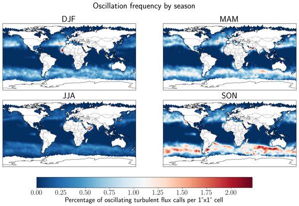
To further characterize the Earth system states associated with oscillations in the ocean–atmosphere flux parameterization, we perform offline calculations using 10 years of four-times-daily instantaneous output from E3SMv2 as mentioned in Sect. 2.5. In these offline calculations, we again apply Algorithm 1 until either the stopping criterion is reached or a maximum of 1000 iterations have been taken. Each data point is classified as either (i) exhibiting oscillatory behavior or (ii) having converged if the stopping criterion is reached. Since the focus here is on cases near neutral stability (ζ=0) and since the stability is controlled in part by U, Δθ, and Δq, normalized histograms of U, Δθ, and Δq values are provided in Fig. 3 for both calls to the turbulent flux algorithm with oscillations and calls that have converged to a solution. One notable observation is that a large majority of calls resulting in oscillations have temperature differentials at near-neutral stability in the range 0–0.7 K. This is perhaps not surprising since the discontinuity in at ζ=0 occurs when Δθ=0 K. In particular, it is not unexpected that small non-zero values of Δθ can cause non-convergence, e.g. due to fixed point iterates near ζ=0 jumping between the two branches of . Figure 4 also shows the geographic distribution of calls resulting in oscillating iterations by season. The most frequent oscillations occur in the Southern Ocean along the ice edge in September, October, and November (hereinafter SON) and in the Arabian Sea in June, July, and August (hereinafter JJA) as well as March, April, and May (hereinafter MAM). Frequent oscillations are also observed off the western coast of Africa in December, January, and February (hereinafter DJF). Moderate frequency of oscillations is observed in the North Atlantic and Southern Oceans in all months.

Figure 4Percentage of turbulent flux calls resulting in oscillating iterations in each 1°×1° cell by season. The displayed data is obtained from 10 years of four-times-daily instantaneous output from E3SMv2. White areas over the oceans indicate sea ice.
3.3 Regularization of heat exchange coefficient to recover solution existence
To enforce continuity of the heat exchange coefficient , we propose a standard Ck regularization which replaces the jump discontinuity with a polynomial function with two parameters k (a non-negative integer) and εreg (a small positive value). The new regularized coefficient, which we denote by , has k continuous derivatives and is defined by
In turn, is used to derive a regularized version of the exchange coefficient , which we denote by and which will take the place of in Eq. (13). Details on the construction of the polynomial and the regularized exchange coefficient are provided in Appendix C. Figure 5 provides a visualization of the polynomial , which corresponds to the case of linear interpolation. Higher-order regularizations which preserve continuity of first and second derivatives are not necessary for the fixed-point iterations used in E3SMv2 which require no information on the derivatives of f. We thus use only the polynomial in Eq. (21) in the rest of this work. However, if higher-order fixed-point solvers are desired, then commensurately higher-order regularizations corresponding to the polynomials and even may be required. Details on the construction of these regularizations are provided in Appendix C for the interested reader.
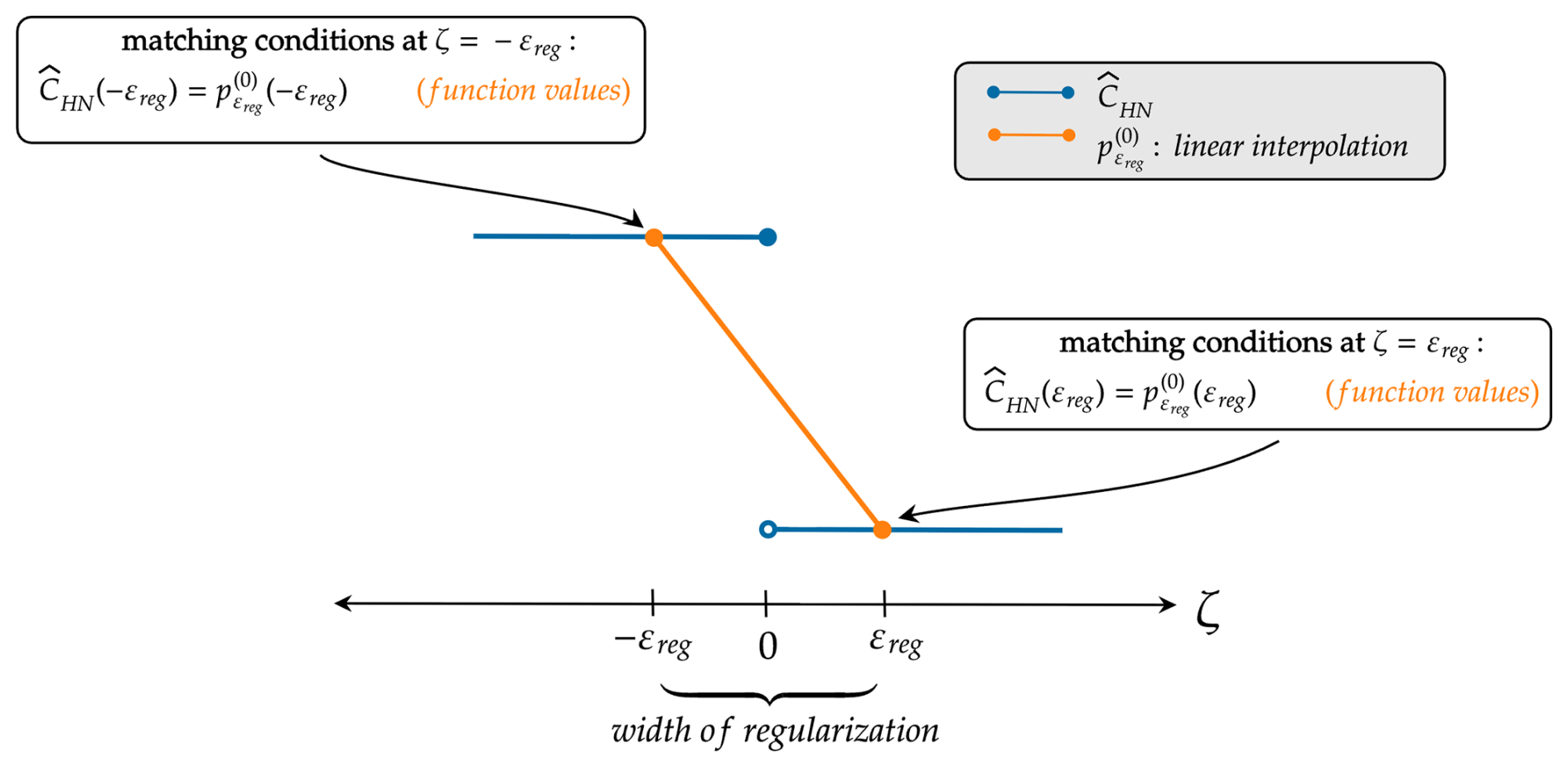
Figure 5Neutral exchange coefficient of heat and its continuous regularization using linear interpolation, . Continuity is enforced by matching the interpolant to the values of at the endpoints of the region of regularization given by .
The regularization parameter εreg determines how much of the original exchange coefficient CHN is replaced by the polynomial . In principle, any positive value of εreg ensures that f is continuous and thus, the turbulent flux parameterization in Eq. (13) has a solution. In practice, smaller values of εreg will preserve more of the original exchange coefficient in Large and Pond (1982) but may not alleviate the problem of oscillating iterations due to the sharp gradient at ζ=0, an issue which we highlight in Sect. 3.4. In contrast, larger values of εreg make it easier for numerical methods to converge to a solution of the regularized equation but modify more of the original exchange coefficient. Thus, care must be taken in choosing εreg so that desirable features of the original exchange coefficient are preserved while also not making it onerously difficult for iterative methods to converge to a solution. A comparison of the convergence of the iterative method as well as differences in the computed turbulent fluxes for various values of εreg is provided in Appendix C. Based on these results, we recommend a value of εreg=0.1, which produces turbulent fluxes that do not differ significantly from the fluxes produced when using a regularization with smaller values of εreg.
3.4 Ensuring convergent iteration for the regularized system
While the goal of the regularization in Sect. 3.3 is to ensure that the system Eq. (13) has at least one solution for iterative methods to converge to, the potentially sharp gradient (depending on how small the regularization parameter εreg is) introduced in the regularization can pose issues for iterative methods such as the fixed-point and nonlinear Gauss-Seidel iterations. In particular, the presence of sharp gradients often necessitates the use of damping (i.e. α<1 in Eq. 16) to reduce the iteration “step size” and prevent over and under-shooting of iterates. To see this, we apply a variant of the default iteration described in Algorithm 1 that (i) takes a fixed 100 iterations and (ii) introduces a damping parameter to compute the solution of the regularized turbulent flux parameterization in Eq. (C3) with εreg=0.1 for the example described by Eq. (20). We consider the damping parameters α= 1, 0.5, and 0.1 and show the results in Fig. 6. It is clear that the damped iteration converges to the solution of the regularized Eq. (C3) so long as the damping parameter is chosen small enough. In particular, if α is too large relative to εreg, the oscillations are still present at varying levels depending on the value of α chosen. In the F2010 simulations described in Sect. 2.2, we fix εreg=0.1 and α=0.016, which allows convergence of the iterations for all meteorological conditions encountered in the 10-year model run according to the convergence criteria discussed next in Sect. 3.5.

Figure 6The iterate (θ*)n and its relative residual when approximating the solution of the regularized turbulent flux parameterization in Eq. (C3) with conditions described by Eq. (20). The value of the regularization parameter is εreg=0.1. The iterates are described by Algorithm 2 with damping parameters chosen from .
3.5 Number of iterations and stopping criterion
Before presenting the full algorithm for numerically solving the regularized turbulent flux parameterization in Eq. (C3), we discuss convergence criteria for terminating the iterative process. The default E3SM iteration described in Algorithm 1 takes two iterations and returns the second iterate as the approximation to the scaling parameters. Standard practice in numerical methods is to have iterative methods, such as the fixed-point iteration, terminate when a convergence test is passed or after a maximum number of iterations maxiter is reached (chosen to be orders of magnitude larger than is expected for the iteration to converge).

Figure 7Analogous histograms to Fig. 3 show distribution of wind speed, temperature differential, and specific humidity differential for atmospheric conditions producing oscillatory, non-convergent iterations (orange bars) and those whose iteration converges to a solution (blue bars) when the regularization in Eq. (21) is utilized with εreg=0.5 and a damping parameter of α=0.08 in the fixed point iteration.
We utilize the same relative residual as in Sect. 3.2, i.e. Eq. (19). Given the iterate , the proposed convergence test is to check whether for a user-prescribed tolerance 𝚝𝚘𝚕>0. The full algorithm for approximating the scaling parameters described by the turbulent flux parameterization in Eq. (C3) is given in Algorithm 2. For the 10-year simulation SENS described in Sect. 2.5, we take and .
To demonstrate the efficacy of the regularized neutral exchange coefficient in removing oscillations in the iterate xn, we perform an offline test on the same 10 years of four-times-daily instantaneous output from the CTRL simulation shown in Fig. 3, this time using Algorithm 2. The corresponding histograms showing classifications of each data point as oscillatory or convergent are presented in Fig. 7. We observe that all sets of meteorological conditions are now able to be driven to the desired residual error tolerance, from which we surmise that the regularization proposed in Sect. 3.3 is sufficient in addressing solution non-existence in the Large and Pond parameterization.
3.6 Comments on computational cost
Finally, we briefly comment on the efficiency of the proposed Algorithm 2 compared to the E3SMv2 default Algorithm 1. One should not generally expect to obtain a high level of accuracy in the scaling parameters (and hence, the turbulent fluxes as well) using the default two iterations described in Algorithm 1. By accuracy, we refer only to the degree to which the computed scaling parameters satisfy Eq. (13). Whether the subsequent turbulent fluxes are physically accurate is uncertain and it is expected that the parameterization itself introduces significant error. On the one hand, developers of E3SM and other ESMs might argue that the level of accuracy achieved with two iterations is on par with the low level of accuracy associated with many other numerical calculations of E3SM, for instance, first-order time integration and coupling methods (Wan et al., 2021, 2015). On the other hand, recent improvements to physics parameterizations and their coupling (e.g., Wan et al., 2024; Zhang et al., 2023) in ESMs means that the relatively large approximation errors associated with Algorithm 1 may start to exceed errors in the other parts of E3SM in future versions of this ESM.
While Algorithm 2 is usually (depending on the value of tol) more computationally expensive than the default E3SMv2 algorithm since more than two iterations are usually required to reach a given tolerance, techniques for accelerating convergence of Algorithm 2 are readily available. For example, Anderson acceleration (Anderson, 1965) updates the iteration by computing a linear combination of m previous iterates and, in many cases, converges faster than the standard fixed-point and Gauss-Seidel iterations. Efficient implementations are available to Fortran and C++ codes via software libraries such as SUNDIALS (Hindmarsh et al., 2005; Gardner et al., 2022). To demonstrate the potential benefits of Anderson acceleration, we solve the equations underlying the regularized turbulent flux parameterization Eq. (C3) in offline calculations using Earth system conditions sampled from the CTRL simulation every five days over the course of one year. Numerical solution of the scaling parameter equations is done using either (i) Anderson acceleration from SUNDIALS with m=1 which computes the update xn+1 using the previous iterates xn and xn−1, or (ii) the standard fixed-point iteration Eq. (16) which has the same computational cost per iteration as the default E3SM iteration in Algorithm 1 (Fig. 8). We observe that Anderson acceleration converges rapidly and also results in significant speed-up in wall clock time in comparison to the standard fixed-point iteration. For instance, Anderson acceleration attains an average relative residual of 10−4 more than three times faster than the standard fixed-point iteration.
Algorithm 2Regularized atmosphere-ocean iteration.
tol; maximum iterations maxiter.tol, maxiter)
Figure 8A demonstration of Anderson acceleration to improve convergence of scaling parameters. (left) Behavior of the relative residual ℛ(xn;ξ) for approximating surface fluxes from the parameterization Eq. (C3) at a single location with 𝚖𝚊𝚡𝚒𝚝𝚎𝚛𝚜=100 and . (right) Average residual for meteorological conditions sampled across a year of data from the CTRL simulation vs. average wall clock time per call. Individual points correspond to fixed-point and Anderson acceleration iterations with and .
With some confidence that a solution now exists to the regularized Large and Pond parameterization described in Sect. 3.3 and its corresponding algorithm in Algorithm 2, we now turn our attention to the issue of solution uniqueness. If the underlying equations have more than one solution, then the iterative method described in Algorithm 2 may converge to different solutions depending on the initial guess.
4.1 Unbounded Obukhov stability parameter produces unintended solution
In this subsection, we demonstrate that the principal driver of solution non-uniqueness is a singularity in the Obukhov stability parameter ζ defined in Eqs. (7) and (11). In particular, due to the presence of u* in its denominator, ζ is undefined when . Likewise, the function f describing the right-hand side of Eq. (13) depends on ζ and is also undefined when . From a practical perspective, this also means that small values of u* may potentially cause ζ to take on extremely large magnitudes.
While ζ is undefined whenever , we may still gain understanding of the behavior of ζ by examining the limiting behavior as . It is important to note that ζ is also a function of θ* and q*, whose values will also vary throughout the application of an iterative method. The limit of such a multivariable function as its input variables approach a particular point exists if and only if the function approaches the same value along every trajectory that approaches the particular point. This means that, depending on how the limit ζ→0 is approached, iterates may converge to different points. Indeed, one can show that along certain trajectories, as (in which case f→0 and thus, the iterates in Eq. (16) converge to 0), while along others, ζ→0 as (in which case and iterates should not converge to 0). More mathematical details may be found in Appendix D

Figure 9Progress of approximating the scaling parameters u*, θ*, and q* and 10 m wind speed, u10N, in Algorithm 2 with and without stability limiter. Each dashed line represents an application of Algorithm 2 with an initial guess drawn randomly from a uniform distribution. Without the limiter, the iterations converge to one of two solutions depending on the initial guess: a trivial one at (orange curves) and a non-trivial solution (blue curves). When the limiter is applied with ζmax=10, as is currently done in E3SM, the trivial solution at is shifted to (grey curves) rather than eliminated.
To see how this ill-defined behavior along different trajectories manifests in practice, we now use offline calculations to demonstrate that certain meteorological conditions indeed result in the situation of iterative methods being able to converge to two different solutions depending on how the initial iterate is chosen. An example of such meteorological conditions for which it is possible that the iterates is
We apply Algorithm 2 100 times without the stability limiter (i.e. is replaced by ζ in Algorithm 2), each with a randomized initial iterate, and plot the scaling parameters at each iteration of the algorithm (Fig. 9). We observe convergence of the iterates to two distinct points for this example – one at corresponding to the case when and another at . Such behavior shows the importance of preventing for the regularized turbulent flux parameterization Eq. (C3), and it supports the idea of limiting ζ in general, although we shall elaborate in the next subsection that the limiter needs to be implemented in a careful way in order to be effective and reliable. We also note that while this issue also persists for the default unregularized parameterization Eq. (13), the experiment presented in Fig. 9 is performed with the regularized turbulent flux parameterization in order to ensure that issues with solution existence are not encountered.
4.2 Role of Obukhov stability limiter in solution non-uniqueness
We now turn our attention to the limited stability parameter and address its role in determining uniqueness of the surface fluxes. Recall that E3SM utilizes the stability limiter (i.e., Eq. 17) in the implementation of Algorithm 1 to prevent the magnitude of ζ from growing to physically unreasonable values, i.e. the scenario where . More than an innocuous numerical treatment, this limiter modifies the mathematical properties of the mapping f. To the best of our knowledge, no systematic analysis has been carried out to determine the effect of the limiter (17) on convergence of Algorithm 1.
One might expect that since the limiter removes the possibility that , iterative methods should not be able to converge to , and Eq. (C3) should have a unique solution when the limiter is applied. However, we demonstrate that while the limiter does prevent convergence of the iterates to , it introduces a shifted “solution” to the system. To see this, we consider the same example described by Eq. (22) but apply the limiter (17) with as in E3SMv2 (Fig. 9). We observe that the “solution” at is shifted to and in fact, the regularized turbulent flux parameterization described by Eq. (C3) has two solutions when the stability limiter is applied.
4.3 Exploring the solution space via bifurcation diagrams
More generally, the value of the limiting parameter ζmax has a strong effect on the number of solutions of Eq. (C3). When an analytic solution of a given equation is known, a systematic analysis of the effect of a model parameter on uniqueness of the solution is straightforward. For instance, one can express the solution as a function of the parameter of interest and generate a bifurcation diagram (Chow and Hale, 2012) which provides qualitative information on the solution for each value of the parameter. Given that an analytic solution of Eq. (C3) is not known, an approximate bifurcation diagram may still be generated by performing several runs of Algorithm 2 for a range of different initial guesses and observing how many distinct solutions the algorithm converges to for different values of ζmax.
Table 1Four different possible scenarios arising from use of limiters on the Obukhov stability parameter. Detailed discussions can be found in Sect. 4.3.

With E3SM's default of ζmax=10 in mind, we examined a large number of meteorological conditions in the CTRL simulation while varying ζmax over a range of values from 10−1 to 104. Based on this analysis, we observed four distinct scenarios regarding solution uniqueness. These scenarios are illustrated in Table 1 alongside examples of the meteorological conditions producing those scenarios. An in-depth explanation of these scenarios is provided below.
-
There is exactly one solution which does not depend on ζmax.
-
There is exactly one solution which varies with ζmax until a turning point after which the solution is constant with ζmax. When the solution varies with ζmax, it is described implicitly by the manifold on which
-
There is exactly one solution which depends on ζmax. This solution is given implicitly by Eq. (23).
-
For ζmax within a certain range, there are exactly two solutions, one of which does not vary with ζmax and one of which varies with ζmax. The latter is described by Eq. (23). For ζmax outside of this range, there is a unique solution which may or may not vary with ζmax. The value of ζmax at which the number of possible solutions transitions from one to two is known as a bifurcation point.
The first scenario is ideal in the sense that the limiter has no effect on the solution. While a rigorous theory establishing precisely when this scenario occurs is beyond the mathematical techniques described in this paper, we suspect that this scenario may occur when the meteorological conditions prevent the stability parameter ζ from taking on large values near the solution.
The second scenario illustrates that the limiter must be chosen carefully in order to ensure that the obtained solution exhibits desirable behavior, namely that the obtained solution should not vary with the value of ζmax. When ζmax≳15, we observe that the solution is constant with respect to ζmax. It is this desired solution which a numerical method should converge to. On the other hand, if ζmax≲15, we observe the undesired behavior in which the solution varies with the value of ζmax. Notably, the current value of ζmax=10 in E3SM is too small in that it would result in obtaining the undesired solution.

Figure 10An example of the adaptive stability limiting process. For the initial limiter, two solutions exist – the desired solution which is constant in ζmax (orange curve) and the second, undesired solution that lies on the manifold described by (blue curve). If the desired solution is obtained by Algorithm 3, there is no need to adjust the limiting parameter ζmax. Otherwise, we incrementally decrease ζmax until a solution satisfying is reached. In this example, the process is guaranteed to terminate once ζmax falls in the approximate interval (0.5,0.8). In general, if the process terminates without finding the desired solution, e.g. because it does not exist (see third scenario in Table 1), then we default to the solution obtained from the default E3SM limiting parameter value of ζmax=10. A more detailed discussion may be found in Sect. 4.4.
The third scenario in which the only solution depends on the value of ζmax suggests that the underlying equations are still ill-posed. In particular, the limiting case when ζmax→∞ may be viewed as equivalent to the case without the stability limiter. Here, the bifurcation diagram suggests that is the only solution, but we have described in the preceding discussion in Sect. 4.1 why is not a solution to Eq. (C3). Thus, it appears that the stability limiter is a necessity in these cases in order for the turbulent flux parameterization to behave in a robust manner.
The fourth scenario, much like the second, illustrates the importance of correctly selecting ζmax to obtain the physically relevant solution. When ζmax≳0.8, there are two solutions to the turbulent flux parameterization Eq. (C3), and Algorithm 2 may converge to either solution depending on the initial guess. For the small interval , only the desired solution that does not vary with ζmax is obtained, and this finding suggests that the value of ζmax should fall in this interval to guarantee convergence of Algorithm 2 to the desired solution.
Lastly, the issue of the limiting parameter value dictating the number of possible solutions to the underlying equations of the Large and Pond turbulent flux parameterization is likely to cause problems with solution uniqueness in other parameterizations as well. For instance, the alternate University of Arizona parameterization (Zeng et al., 1998) was implemented into E3SMv2 as a possible alternative to the Large and Pond parameterization with the same limiters described by Eq. (17). The COAREv3 parameterization (Fairall et al., 2003), on the other hand, does not utilize limiters on the stability parameter. However, when stability limiters are not applied, one may view this as the asymptotic case when ζmax→∞ in Fig. 10; in this case, it is still possible for the underlying equations to have two solutions (cf. Fig. 9) although we have not explored this possibility for any parameterizations aside from that of Large and Pond.
4.4 Adaptive selection of limiting parameters
The preceding discussions in Sect. 4.2 and 4.3 suggest that there is no single value of ζmax that will ensure the existence of only one solution to the turbulent flux parameterization for all meteorological conditions. For instance, for the meteorological conditions described in the fourth scenario in Table 1, a value of ζmax=0.6 is appropriate but would result in obtaining an undesired solution if the same value is used for the meteorological conditions described in the second scenario in Table 1.
Instead, we propose utilizing an adaptive stability limiter in which the value of ζmax is permitted to vary based on the meteorological conditions. The key idea is to begin with an initial maximum value of ζmax and apply Algorithm 2 to obtain a first approximation of the scaling parameters u*, θ*, and q*. If the value of the stability parameter associated with scaling parameters, , is equal to ζmax, we decrease the value of ζmax and apply Algorithm 2 until scaling parameters are obtained for which . A visualization of this procedure is provided in Fig. 10. The complete turbulent flux algorithm with adaptive stability limiter is presented in Algorithm 3.
Algorithm 3Modified atmosphere-ocean iteration for uniqueness.
tol; maximum iterations maxiter.tol, maxiter)tol, maxiter).tol, maxiter).When the adaptive approach is unable to find a desired solution, e.g. the third scenario in Table 1, we elect to leave the limiting parameter at its default value of ζmax=10. As previously mentioned, this scenario suggests that the underlying equations are ill-posed without the fallback limiter in place. Whether this issue is caused by violation of the underlying physical assumptions of the parameterization (e.g. extremely stable atmospheric conditions) or breakdown in the algorithmic formulation is difficult to ascertain and beyond the scope of this work. Instead, we note that the limiter appears necessary in these cases to restore well-posedness of the parameterization. A quantification of how often calls to the original and revised turbulent flux algorithms result in solutions with is provided in Sect. 4.5.
The computational cost of Algorithm 3 is dependent on the initial value of ζmax. An exploration of the sensitivity of the overall Earth system to the choice of ζmax is provided in Appendix E. We only note here that the choice ζmax=200 appears to be sufficient for Algorithm 3 to return scaling parameters satisfying when possible.
4.5 Occurrence of undesired solutions in E3SM
The preceding discussion highlights the issues associated with the stability limiter (17). In particular, current implementations of ocean–atmosphere turbulent flux algorithms may potentially converge to undesired solutions on the manifold . To better understand the physical conditions producing when ζmax is fixed at E3SMv2's value of 10, we again consider ten years of data from the CTRL simulation. We apply the default Algorithm 1 with 100 iterations instead of 2 iterations and categorize each spatial location based on the value of ζ. Figure 11 shows the distribution of meteorological conditions when and when . The clearest distinction between the two cases is that locations for which have relatively small wind speeds of less than 2 m s−1. As in the case of oscillating turbulent flux iterations being associated with near neutral stability, the occurrences of being tied to low wind speed is also not unexpected since the stability parameter blows up when u*, which is proportional to U, tends to 0. Such conditions are most frequent around the Equator, especially across the Indian Ocean, as shown in Fig. 12.


Figure 12Percentage of turbulent flux calls resulting in in each 1°×1° cell. The displayed data is obtained from ten years of four-times-daily instantaneous output from the CTRL simulation. The condition indicates that the surface fluxes lie on the manifold of solutions to (C3) which would vary with ζmax. Different panels correspond to different seasons. White areas over the oceans indicate sea ice. Further details can be found in Sect. 4.5.
Table 2Comparison of number of non-convergent turbulent flux calls and number of calls with for the default algorithm (Algorithm 1) and the revised algorithm (Algorithm 3) using 10 years of four-times-daily instantaneous data from E3SMv2 CTRL simulation. Total number of calls to each algorithm across the entire data set is 183 589 464.

Lastly, we examine the efficacy of the revised turbulent flux algorithm in restoring convergence and preventing convergence to undesired solutions in an offline test of 10 years of four-times-daily instantaneous data from E3SMv2. Table 2 shows the number of turbulent flux calls resulting in non-convergent iterations as well as calls resulting in solutions with . We observe that the revised scheme is able to entirely restore convergence to non-convergent calls and reduces the frequency of solutions on the manifold by almost 90 %. The remaining calls with are entirely due to the fallback limiter being invoked in Algorithm 3.
We perform a pair of 10-year simulations – CTRL and SENS described in Sect. 2.5 – to investigate the sensitivity of E3SM to the proposed changes in Algorithm 3. For SENS, a tolerance of is used for the stopping criterion with a maximum permissible number of iterations ; the value of maxiter is arbitrarily chosen to be significantly larger than expected to reach the specified tolerance. A C0 regularization is used to enforce continuity of the exchange coefficient with εreg=0.1. A damping value of α=0.016 is employed in the iteration. Lastly, an initial stability limiting parameter of ζmax=200 is used with an increment of ζincr=0.25 in the adaptive limiting process.
When analyzing the simulation results, one must distinguish impacts of the regularization and the revisions in the numerical algorithm from noise caused by natural variability and other sources of uncertainty in the model. To determine whether differences in the 10-year mean fluxes are statistically significant, a one-sample Student's t-test is performed using monthly mean output data. Since the data are serially correlated, we utilize a revised t-test in which the t statistic is scaled by an effective sample size (Zwiers and von Storch, 1995). A significance level of 0.05 is utilized to determine when the mean of the differences is likely to be non-zero.

Figure 13The 10-year mean latent heat flux (left), sensible heat flux (middle), and wind stress (right) for the months of DJF (upper row), as well as the difference between the CTRL and SENS simulations (bottom row) in which statistically insignificant differences are masked out in white.

Figure 14The 10-year mean latent heat flux (left), sensible heat flux (middle), and wind stress (right) for the months of JJA (upper row), as well as the difference between the CTRL and SENS simulations (bottom row) in which statistically insignificant differences are masked out in white.
The largest effects on turbulent fluxes occur in DJF (Fig. 13) and JJA (Fig. 14), while the effects in other months are substantially smaller. Statistically significant latent heat flux differences exceeding 10 W m−2 in magnitude and sensible heat flux differences exceeding 6 W m−2 in magnitude can be found in several regions, mainly over the oceans of the winter hemisphere including over the Gulf of Alaska and over the Labrador Sea in DJF and over the Southern Ocean in JJA. Smaller but still statistically significant differences in latent heat fluxes are found in tropical and subtropical areas. The changes in atmospheric circulation, temperature, and humidity are small in terms of 10-year averages, but we note that in the future, it will be useful to perform fully coupled Earth system simulations to assess whether larger impacts will be seen when the atmosphere and ocean components can interact with each other.
We also performed additional sensitivity experiments using regularization parameters larger or smaller than εreg=0.1. These results can be found in Appendix C, Fig. C2. Within the tested range of εreg=0.015 to 0.5, the overall results from E3SM, in terms of 10-year averages, are not substantially different from what is presented here in Figs. 13 and 14.
Table 3Summary of well-posedness findings in the turbulent flux parameterization in E3SMv2 based on Large and Pond (1981) and Large and Pond (1982).

In this study, we have analyzed the solvability of the underlying equations of an ocean–atmosphere turbulent flux parameterization that is based on measurements discussed in Large and Pond (1981, 1982) and is used by a number of ESMs, e.g., E3SM, CESM, TaiESM, NorESM, CMCC-ESM2, and RASM. Our analysis has shown that there are certain meteorological conditions, mostly encountered over the mid-latitude oceans under stable conditions, for which the turbulent flux algorithm implemented in E3SMv2 is unable to converge to a solution. This non-convergence manifests as oscillations of the scaling parameter iterates and results in a rather large residual error (>50 % on average). The likely causal factor of non-convergence is a discontinuity in the neutral heat exchange coefficient. Moreover, we have shown that this turbulent flux algorithm does not always yield unique surface fluxes and the use of an ad hoc limiter on the Monin-Obukhov length has a strong influence on the number of solutions. Meteorological conditions that produce non-unique solutions are found mostly in regions with low wind speed near the Equator.
We have introduced two modifications to the Large and Pond parameterization in order to enforce both existence and uniqueness of the computed surface fluxes. These modifications include (i) regularization of the discontinuous neutral exchange coefficient for heat, which resolves issues with oscillating surface fluxes corresponding to large residual errors, and (ii) adaptive selection of the limiter on the Monin-Obukhov length to eliminate unintended solutions when the numerical solutions are not unique. A summary of these issues and their remedies is provided in Table 3.
Sensitivity of E3SMv2's mean climate to these issues of well-posedness was investigated by comparing 10-year simulations using the default formulation and algorithm (see Eq. 14, Appendix A, and Algorithm 1) as well as the regularized formulation and revised algorithm (Sect. 3.3, Appendix C, and Algorithm 3). The modifications lead to statistically significant differences in the 10-year mean latent and sensible heat fluxes compared to those of the default model, exceeding 10 and 6 W m−2 in magnitudes, respectively, in various regions.
While the impacts of the revised flux algorithm on the simulated 10-year mean atmospheric circulation, temperature, and humidity are relatively small, it will be worth performing fully coupled Earth system simulations in the future to assess whether there will be larger impacts when the atmosphere and ocean components of E3SM can interact with each other. The analysis in this study demonstrates a strategy for future investigations of other ocean–atmosphere flux parameterization options in E3SM, such as the Coupled Ocean–Atmosphere Response Experiment (COARE, Fairall et al., 2003) and the University of Arizona (UA, Zeng et al., 1998) parameterizations. Furthermore, turbulent flux algorithms over sea ice and land share many similarities with the ocean–atmosphere algorithms since they too are based on MOST. They may also include discontinuous exchange coefficients in certain scenarios as well as ad hoc use of stability limiters as seen here in the ocean–atmosphere algorithm, which will be subjects of future research.
Beyond the topic of turbulent flux parameterizations at the Earth's surface, it is worth noting that many parameterization codes include discontinuities to distinguish between regimes, and employ limiters to avoid singularities or constrain values to physically plausible ranges. Model developers who focus primarily on the simulated physics may not always be aware that these discontinuities and limiters can significantly influence simulation outcomes, or that well-established mathematical techniques exist to address the underlying needs for such constructs, for instance polynomial regularization and bifurcation analysis in this paper. Some of these methods are straightforward to implement and need not incur prohibitive computational costs, as demonstrated in this study. Raising awareness of well-posedness issues in parameterizations – and of the computational techniques available to address them – is therefore a key contribution of this paper, perhaps as important as the specific improvements made to the ocean–atmosphere turbulent flux parameterization in E3SMv2.
In this section, we first clarify the expression of the exchange coefficients C(D,H,E) (Appendix A1) and then describe their adjustment to measurement height and stability which is utilized in the E3SMv2 code (Appendix A2).
A1 Exchange coefficients
The parameterization used in E3SMv2 is based on the work of Large and Pond (1981) and Large and Pond (1982) which provide expressions for CD, CH and CE in terms of neutral exchange coefficients CDN, CHN, CEN (see Eq. 15 in Large and Pond, 1981 and Eq. 10 in Large and Pond, 1982). These expressions are as follows:
Here, zref=10 m is the reference height. The dimensionless stability functions ψm, ψh, and ψq are defined in terms of the Obukhov stability parameter ζ and are as follows (Large, 2006, Eq. 20):
where (see Eq. 20 in Large, 2006 but note that the parentheses therein need to be replaced by an absolute value sign). The stability functions ψm, ψh, and ψq are continuous at ζ=0 despite their piecewise definitions. The neutral exchange coefficients are defined as follows.
-
For momentum (Large, 2006, Eq. 34),
-
For heat (Large and Pond, 1982, Eq. 23),
-
For moisture (Large and Pond, 1982, Eq. 24),
We see from Eqs. (A1)–(A3) that the exchange coefficients are functions of u10N, ζ, and z (represented by the bulk meteorological variables ξ), i.e.,
A2 Nonlinear equation solved in E3SMv2
Neglecting wind gustiness (i.e., assuming S=U) and combining Eqs. (4)–(6) with Eqs. (8)–(10) to eliminate the eddy covariances, we obtain
We introduce the new set of symbols to denote the adjusted exchange coefficients which are defined by
and write Eq. (A10) as
The definitions of in Eq. (A11) may be expanded using Eqs. (A1)–(A3) to obtain
where the adjusted neutral exchange coefficients and no longer depend on the neutral 10 m wind speed and are given by
Finally, the neutral 10 m wind speed is itself a function of the friction velocity u* and CDN and is given by the nonlinear equation
Equation (A15) together with Eq. (A12) constitutes the nonlinear system of equations as implemented in E3SMv2.
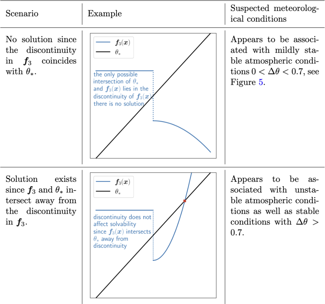
Discontinuities in the neutral exchange coefficient CHN can cause Eq. (13) to have no solutions. However, the presence of the discontinuity is not in itself a guarantee of solution non-existence. Table B1 shows two possible scenarios with abstract illustrations in one dimension to demonstrate when the discontinuity causes solution non-existence. Based on offline analysis of the 10-year CTRL simulation described in Sect. 2.5, we are able to link each of the scenarios in Table B1 to different stability regimes in the atmosphere. In particular, it appears (see Fig. 3) that the discontinuity only causes solution non-existence under mildly stable atmospheric conditions while unstable conditions as well as stable conditions with Δθ>0.7 do not pose any issues to solution existence.
Table B1A graphical visualization of the existence or non-existence of a solution to the Large and Pond turbulent flux parameterization Eq. (13) due to the discontinuity in the neutral heat exchange coefficient . We focus on the third equation of Eq. (15) which contains the discontinuity and may be written as .
The discontinuous neutral heat exchange coefficient is replaced by the regularized coefficient
The polynomial is given by
where the coefficients, aj, are obtained by enforcing the continuity conditions
which amounts to solving a system of 2k+2 linear equations.
For the fixed-point and nonlinear Gauss-Seidel iterations employed by E3SM, enforcing C0 continuity – i.e. continuity of just – is enough to allow these methods to converge. However, we have provided the polynomial regularization for enforcing general continuity of up to order k derivatives since higher-order iterative methods such as Newton's method require C1 or even stronger continuity of the right-hand side function f. For completeness, we state the C0 and C1 polynomials below:
With the regularized neutral heat exchange coefficient , we may define a corresponding regularized heat exchange coefficient :
Finally, the regularized turbulent flux parameterization based on the Large and Pond (1982) parameterization is given by
The effect of the regularization parameter εreg on the convergence of iterations is shown in Fig. C1 for the meteorological conditions described by Eq. (20). As discussed in Sect. 3.3, the particular construction of the regularized neutral heat exchange coefficient (21) means that smaller values of εreg introduce sharper gradients to f which require smaller values of the damping parameter α to resolve in Algorithm 2. Indeed, we observe nearly an order of magnitude increase in the number of iterations required to reach a relative residual of 10−12 for each order of magnitude decrease in εreg.
To determine the effect of the regularization parameter on the overall Earth system, we consider the differences between the CTRL latent and sensible heat fluxes and wind stress, which are computed using the default E3SMv2 algorithm (Algorithm 1) without any modifications to address solution non-existence and non-uniqueness, and the corresponding fluxes obtained from a sequence of simulations with and a fixed ζmax=200 (Algorithm 3). The CTRL and regularized turbulent fluxes are not substantially different as εreg is decreased. For this reason, we suggest taking εreg=0.1 to capture the most significant changes resulting from the regularization.


Figure C210-year mean differences in latent heat flux (top row), sensible heat flux (middle row), and wind stress (bottom row) between CTRL simulation and a sequence of simulations with (from left to right). The initial adaptive stability limiter described in Sect. 4.4 is fixed at ζmax=20.
We consider the multivariable limiting behavior , where, in addition to , we are also interested in the case when θ* and q* simultaneously approach 0.
In what may seem like a purely academic exercise at first, we demonstrate that the limiting behavior of ζ is different depending on the trajectory taken towards . We will express u*, θ*, and q* using a dummy variable s so that the limiting behavior may be examined as s→0 instead – that is, .
A basic result from multivariable calculus states that the limit of a multivariable function as its input variables approach a particular point exists if and only if the function approaches the same value along every trajectory that approaches the particular point. We show here that it is possible to construct two trajectories along which ζ converges to different values, and explain the expected implication of each case on the turbulent flux Algorithms 1 and 2.
-
The first trajectory is described by , , and . By evaluating the limit along this trajectory using Eq. (7) and the definition of the trajectory, we can see that . Whenever , we can see by inspection of the stability functions ψ(m,h,q) (see Eqs. A4–A5) and exchange coefficients (see Eqs. A1–A3 and their regularized variants in Eq. A11) that the right-hand side of the turbulent flux parameterization Eq. (13) approaches 0. In other words, along this kind of trajectory, the residual of Eq. (13) decays to 0. We expect that numerically, serves as a secondary “solution” that iterative methods may converge to if they approach a trajectory such as the one described here.
-
The second trajectory is described by , , and , from which we see that
. In other words, the right-hand side of Eq. (13) is finite and nonzero, and the residual of Eq. (13) does not decay to 0. This case demonstrates the existence of trajectories along which iterative methods will not converge to .
In summary, the Obukhov stability parameter may become unbounded due to division by u* in its definition. When iterations produced by iterative methods fall along certain trajectories, we expect that they may converge to , which serves as a secondary “solution” to Eq. (13). However, according to the multivariate calculus result stated earlier, because ζ can approach distinct values (e.g., +∞ and 0) when different trajectories are taken towards , the point is not an actual solution to Eq. (13), hence it is problematic that an iterative method may converge to this point. Furthermore, it is worth noting that the danger of converging to can be seen from the continuous formulation of the parameterization; hence, using a different numerical algorithm might not automatically avoid this danger unless deliberate design features are introduced, as we discuss in Sect. 4.4.
The adaptive limiter described in Sect. 4.4 requires one to select an initial value of ζmax, which is then decreased if no suitable solution is found that satisfies . In certain scenarios, for instance the second panel of Table 1, the initial value of ζmax must be sufficiently large in order for the system of equations describing the ocean–atmosphere turbulent fluxes to have a solution that does not vary with ζmax. If ζmax is chosen too small, the adaptive limiting algorithm may terminate without finding a solution for which . To this end, we perform a numerical experiment in which the value of the regularization parameter, εreg, is held fixed and the initial limiting parameter is varied. A reference simulation is generated with ζmax=1000 and the latent and sensible heat fluxes are compared with those from a sequence of simulations with ζmax=20 and 200 (Fig. E1). We observe that an initial limiting parameter value of ζmax=200 allows Algorithm 3 to return the same turbulent fluxes as an initial value of ζmax=1000. We thus recommend ζmax=200 in Algorithm 3.
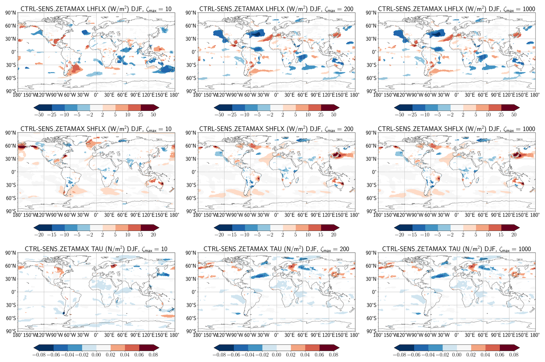
Figure E110-year mean differences in latent heat flux (top row), sensible heat flux (middle row), and wind stress (bottom row) between CTRL simulation and a sequence of simulations with (from left to right). The regularization parameter εreg is fixed at 0.5.
Simulation output data corresponding to the CTRL and SENS simulations and sensitivity runs in Appendices C and E may be found in https://doi.org/10.5281/zenodo.17498126 (Dong et al., 2026b), https://doi.org/10.5281/zenodo.17498147 (Dong et al., 2026c), and https://doi.org/10.5281/zenodo.17510833 (Dong et al., 2026d). Python scripts used to generate bifurcation diagrams, create corner plots, and analyze convergence of the turbulent flux algorithms may be found in https://doi.org/10.5281/zenodo.17511114 (Dong et al., 2026a). A fork of E3SMv2 containing the proposed changes to E3SM's ocean–atmosphere turbulent flux algorithm in Algorithm 3 may be found at the repository https://doi.org/10.5281/zenodo.18180192 (Dong, 2026).
XZ and CSW initiated this study. JD evaluated the Large and Pond algorithm for issues of existence and uniqueness. JD developed and implemented the regularization, damped fixed-point iteration, and adaptive stability limiter with contribution from CSW and CJV. JD performed the CTRL and SENS simulations using E3SM and processed the simulation output; MAB, XZ, and HW contributed to the analysis of the results. JD performed and analyzed offline calculations using E3SM simulation output provided by HW. JD led the writing of this paper with input from all co-authors.
The contact author has declared that none of the authors has any competing interests.
Publisher's note: Copernicus Publications remains neutral with regard to jurisdictional claims made in the text, published maps, institutional affiliations, or any other geographical representation in this paper. The authors bear the ultimate responsibility for providing appropriate place names. Views expressed in the text are those of the authors and do not necessarily reflect the views of the publisher.
The authors would like to thank Sean P. Santos for helpful discussions and feedback in the writing of this manuscript; Kezhen Chong for her guidance in post-processing E3SM simulation data; Arshia Singhal for her initial investigation of the use of Anderson acceleration techniques for computing turbulent fluxes; and Sean P. Santos and Philip J. Rasch for their assistance in identifying current Earth system models that utilize the Large and Pond turbulent flux parameterization.
This research used resources of the National Energy Research Scientific Computing Center (NERSC), a U.S. Department of Energy Office of Science User Facility located at Lawrence Berkeley National Laboratory, operated under Contract No. DE-AC02-05CH11231 using NERSC award ASCR-ERCAP0028881.
This work was performed under the auspices of the U.S. Department of Energy by Lawrence Livermore National Laboratory under Contract DE-AC52-07NA27344. LLNL-JRNL-2001306. Pacific Northwest National Laboratory is operated for the U.S. Department of Energy by Battelle Memorial Institute under contract DE-AC06-76RLO1830.
This material is based upon work supported by the U.S. Department of Energy, Office of Science, Office of Advanced Scientific Computing Research (ASCR), Office of Biological and Environmental Research (BER), Scientific Discovery through Advanced Computing (SciDAC) program, via an ASCR-BER partnership in Earth System Model Development; and by the U.S. Department of Energy, Office of Science, ASCR via the Frameworks, Algorithms, and Software Technologies for Mathematics SciDAC Institute program.
This paper was edited by Riccardo Farneti and reviewed by Charles Pelletier and one anonymous referee.
Anderson, D. G.: Iterative procedures for nonlinear integral equations, J. ACM, 12, 547–560, 1965. a
Banach, S.: Sur les opérations dans les ensembles abstraits et leur application aux équations intégrales, Fund. Math., 3, 133–181, https://doi.org/10.4064/fm-3-1-133-181, 1922. a
Beljaars, A. C. M.: The parametrization of surface fluxes in large-scale models under free convection, Q. J. Roy. Meteor. Soc., 121, 255–270, https://doi.org/10.1002/qj.49712152203, 1995. a, b
Bentsen, M., Bethke, I., Debernard, J. B., Iversen, T., Kirkevåg, A., Seland, Ø., Drange, H., Roelandt, C., Seierstad, I. A., Hoose, C., and Kristjánsson, J. E.: The Norwegian Earth System Model, NorESM1-M – Part 1: Description and basic evaluation of the physical climate, Geosci. Model Dev., 6, 687–720, https://doi.org/10.5194/gmd-6-687-2013, 2013. a
Brodeau, L., Barnier, B., Gulev, S. K., and Woods, C.: Climatologically Significant Effects of Some Approximations in the Bulk Parameterizations of Turbulent Air–Sea Fluxes, J. Phys. Oceanogr., 47, 5–28, https://doi.org/10.1175/JPO-D-16-0169.1, 2017. a
Brunke, M. A., Zeng, X., and Anderson, S.: Uncertainties in sea surface turbulent flux algorithms and data sets, J. Geophys. Res.-Oceans, 107, 5–1–5–21, https://doi.org/10.1029/2001JC000992, 2002. a
Brunke, M. A., Fairall, C. W., Zeng, X., Eymard, L., and Curry, J. A.: Which Bulk Aerodynamic Algorithms are Least Problematic in Computing Ocean Surface Turbulent Fluxes?, J. Climate, 16, 619–635, https://doi.org/10.1175/1520-0442(2003)016<0619:WBAAAL>2.0.CO;2, 2003. a, b, c
Cassano, J. J., DuVivier, A., Roberts, A., Abel, M. R., Seefeldt, M., Brunke, M., Craig, A., Fisel, B., Gutowski, W., Hamman, J., Higgins, M., Maslowski, W., Nijssen, B., Osinski, R., and Zeng, X.: Development of the Regional Arctic System Model (RASM): Near-Surface Atmospheric Climate Sensitivity, J. Climate, 30, 5729–5753, https://doi.org/10.1175/JCLI-D-15-0775.1, 2017. a
Chang, H.-R. and Grossman, R. L.: Evaluation of bulk surface flux algorithms for light wind conditions using data from the Coupled Ocean-Atmosphere Response Experiment (COARE), Q. J. Roy. Meteor. Soc., 125, 1551–1588, https://doi.org/10.1002/qj.49712555705, 1999. a
Chow, S.-N. and Hale, J. K.: Methods of bifurcation theory, vol. 251, Springer Science & Business Media, https://doi.org/10.1007/978-1-4613-8159-4, 2012. a
Danabasoglu, G., Lamarque, J.-F., Bacmeister, J., Bailey, D. A., DuVivier, A. K., Edwards, J., Emmons, L. K., Fasullo, J., Garcia, R., Gettelman, A., Hannay, C., Holland, M. M., Large, W. G., Lauritzen, P. H., Lawrence, D. M., Lenaerts, J. T. M., Lindsay, K., Lipscomb, W. H., Mills, M. J., Neale, R., Oleson, K. W., Otto-Bliesner, B., Phillips, A. S., Sacks, W., Tilmes, S., van Kampenhout, L., Vertenstein, M., Bertini, A., Dennis, J., Deser, C., Fischer, C., Fox-Kemper, B., Kay, J. E., Kinnison, D., Kushner, P. J., Larson, V. E., Long, M. C., Mickelson, S., Moore, J. K., Nienhouse, E., Polvani, L., Rasch, P. J., and Strand, W. G.: The Community Earth System Model Version 2 (CESM2), J. Adv. Model. Earth Sy., 12, e2019MS001916, https://doi.org/10.1029/2019MS001916, 2020. a
Dong, J.: PAESCAL-SciDAC5/E3SM-fork: Ocean atmosphere turbulent flux revisions v2 (ocean_atm_flux_paper_v2), Zenodo [code], https://doi.org/10.5281/zenodo.21325962, 2026. a
Dong, J., Brunke, M. A., Zeng, X., Woodward, C. S., Vogl, C. J., and Wan, H.: E3SMv2 offline analysis of ocean-atmosphere turbulent flux parameterization, Zenodo [data set], https://doi.org/10.5281/zenodo.21333050, 2026a. a
Dong, J., Brunke, M. A., Zeng, X., Woodward, C. S., Wan, H., and Vogl, C. J.: E3SMv2 climatology and time series output for analysis of ocean-atmosphere turbulent flux parameterization (pt 1), Zenodo [data set], https://doi.org/10.5281/zenodo.21833782, 2026b. a
Dong, J., Brunke, M. A., Zeng, X., Woodward, C. S., Wan, H., and Vogl, C. J.: E3SMv2 climatology and time series output for analysis of ocean-atmosphere turbulent flux parameterization (pt 2), Zenodo [data set], https://doi.org/10.5281/zenodo.21834625, 2026c. a
Dong, J., Brunke, M. A., Zeng, X., Woodward, C. S., Wan, H., and Vogl, C. J.: E3SMv2 climatology and time series output for analysis of ocean-atmosphere turbulent flux parameterization (pt 3), Zenodo [data set], https://doi.org/10.5281/zenodo.21841362, 2026d. a
ECMWF: IFS Documentation CY50R1 – Part 4: Physical Processes, ECMWF, https://doi.org/10.21957/49928f2338, 2026. a
Fairall, C. W., Bradley, E. F., Hare, J. E., Grachev, A. A., and Edson, J. B.: Bulk Parameterization of Air–Sea Fluxes: Updates and Verification for the COARE Algorithm, J. Climate, 16, 571–591, https://doi.org/10.1175/1520-0442(2003)016<0571:BPOASF>2.0.CO;2, 2003. a, b, c, d
Gardner, D. J., Reynolds, D. R., Woodward, C. S., and Balos, C. J.: Enabling new flexibility in the SUNDIALS suite of nonlinear and differential/algebraic equation solvers, ACM T. Math. Softw., 48, 1–24, https://doi.org/10.1145/3539801, 2022. a
Golaz, J.-C., Van Roekel, L. P., Zheng, X., Roberts, A. F., Wolfe, J. D., Lin, W., Bradley, A. M., Tang, Q., Maltrud, M. E., Forsyth, R. M., Zhang, C., Zhou, T., Zhang, K., Zender, C. S., Wu, M., Wang, H., Turner, A. K., Singh, B., Richter, J. H., Qin, Y., Petersen, M. R., Mametjanov, A., Ma, P.-L., Larson, V. E., Krishna, J., Keen, N. D., Jeffery, N., Hunke, E. C., Hannah, W. M., Guba, O., Griffin, B. M., Feng, Y., Engwirda, D., Di Vittorio, A. V., Dang, C., Conlon, L. M., Chen, C.-C.-J., Brunke, M. A., Bisht, G., Benedict, J. J., Asay-Davis, X. S., Zhang, Y., Zhang, M., Zeng, X., Xie, S., Wolfram, P. J., Vo, T., Veneziani, M., Tesfa, T. K., Sreepathi, S., Salinger, A. G., Reeves Eyre, J. E. J., Prather, M. J., Mahajan, S., Li, Q., Jones, P. W., Jacob, R. L., Huebler, G. W., Huang, X., Hillman, B. R., Harrop, B. E., Foucar, J. G., Fang, Y., Comeau, D. S., Caldwell, P. M., Bartoletti, T., Balaguru, K., Taylor, M. A., McCoy, R. B., Leung, L. R., and Bader, D. C.: The DOE E3SM Model Version 2: Overview of the Physical Model and Initial Model Evaluation, J. Adv. Model. Earth Sy., 14, e2022MS003156, https://doi.org/10.1029/2022MS003156, 2022. a, b, c
Hannah, W. M., Bradley, A. M., Guba, O., Tang, Q., Golaz, J.-C., and Wolfe, J.: Separating Physics and Dynamics Grids for Improved Computational Efficiency in Spectral Element Earth System Models, J. Adv. Model. Earth Sy, 13, e2020MS002419, https://doi.org/10.1029/2020MS002419, 2021. a
Harrop, B. E., Ma, P.-L., Rasch, P. J., Neale, R. B., and Hannay, C.: The Role of Convective Gustiness in Reducing Seasonal Precipitation Biases in the Tropical West Pacific, J. Adv. Model. Earth Sy., 10, 961–970, https://doi.org/10.1002/2017MS001157, 2018. a
Hartung, K., Svensson, G., Struthers, H., Deppenmeier, A.-L., and Hazeleger, W.: An EC-Earth coupled atmosphere–ocean single-column model (AOSCM.v1_EC-Earth3) for studying coupled marine and polar processes, Geosci. Model Dev., 11, 4117–4137, https://doi.org/10.5194/gmd-11-4117-2018, 2018. a
Hindmarsh, A. C., Brown, P. N., Grant, K. E., Lee, S. L., Serban, R., Shumaker, D. E., and Woodward, C. S.: SUNDIALS: Suite of nonlinear and differential/algebraic equation solvers, ACM T. Math. Softw., 31, 363–396, https://doi.org/10.1145/1089014.1089020, 2005. a
Hurrell, J. W., Holland, M. M., Gent, P. R., Ghan, S., Kay, J. E., Kushner, P. J., Lamarque, J.-F., Large, W. G., Lawrence, D., Lindsay, K., Lipscomb, W. H., Long, M. C., Mahowald, N., Marsh, D. R., Neale, R. B., Rasch, P., Vavrus, S., Vertenstein, M., Bader, D., Collins, W. D., Hack, J. J., Kiehl, J., and Marshall, S.: The Community Earth System Model: A Framework for Collaborative Research, B. Am. Meteorol. Soc., 94, 1339–1360, https://doi.org/10.1175/BAMS-D-12-00121.1, 2013. a
Isaacson, E. and Keller, H. B.: Analysis of numerical methods, Courier Corporation, ISBN 9780486680293, 1994. a, b
Kara, A. B., Rochford, P. A., and Hurlburt, H. E.: Efficient and Accurate Bulk Parameterizations of Air–Sea Fluxes for Use in General Circulation Models, J. Atmos. Ocean. Tech., 17, 1421–1438, https://doi.org/10.1175/1520-0426(2000)017<1421:EAABPO>2.0.CO;2, 2000. a, b
Kara, A. B., Hurlburt, H. E., and Wallcraft, A. J.: Stability-Dependent Exchange Coefficients for Air–Sea Fluxes, J. Atmos. Ocean. Tech, 22, 1080–1094, https://doi.org/10.1175/JTECH1747.1, 2005. a, b
Kawai, H., Yoshida, K., Koshiro, T., and Yukimoto, S.: Importance of Minor-Looking Treatments in Global Climate Models, J. Adv. Model. Earth Sy., 14, e2022MS003128, https://doi.org/10.1029/2022MS003128, 2022. a
Large, W. B.: Surface Fluxes for Practitioners of Global Ocean Data Assimilation, Springer Netherlands, Dordrecht, 229–270, ISBN 978-1-4020-4028-3, https://doi.org/10.1007/1-4020-4028-8_9, 2006. a, b, c, d
Large, W. G. and Caron, J. M.: Diurnal cycling of sea surface temperature, salinity, and current in the CESM coupled climate model, J. Geophys. Res.-Oceans, 120, 3711–3729, https://doi.org/10.1002/2014JC010691, 2015. a
Large, W. G. and Pond, S.: Open Ocean Momentum Flux Measurements in Moderate to Strong Winds, J. Phys. Oceanogr., 11, 324–336, https://doi.org/10.1175/1520-0485(1981)011<0324:OOMFMI>2.0.CO;2, 1981. a, b, c, d, e, f, g
Large, W. G. and Pond, S.: Sensible and latent heat flux measurements over the ocean, J. Phys. Oceanogr., 12, 464–482, https://doi.org/10.1175/1520-0485(1982)012<0464:SALHFM>2.0.CO;2, 1982. a, b, c, d, e, f, g, h, i, j, k, l, m, n
Lee, W.-L., Wang, Y.-C., Shiu, C.-J., Tsai, I., Tu, C.-Y., Lan, Y.-Y., Chen, J.-P., Pan, H.-L., and Hsu, H.-H.: Taiwan Earth System Model Version 1: description and evaluation of mean state, Geosci. Model Dev., 13, 3887–3904, https://doi.org/10.5194/gmd-13-3887-2020, 2020. a
Louis, J.-F.: A parameteric model of vertical eddy fluxes in the atmosphere, Bound.-Lay. Meteorol., 17, 187–202, https://doi.org/10.1007/BF00117978, 1979. a
Lovato, T., Peano, D., Butenschön, M., Materia, S., Iovino, D., Scoccimarro, E., Fogli, P. G., Cherchi, A., Bellucci, A., Gualdi, S., Masina, S., and Navarra, A.: CMIP6 Simulations With the CMCC Earth System Model (CMCC-ESM2), J. Adv. Model. Earth Sy., 14, e2021MS002814, https://doi.org/10.1029/2021MS002814, 2022. a
Ma, P.-L., Harrop, B. E., Larson, V. E., Neale, R. B., Gettelman, A., Morrison, H., Wang, H., Zhang, K., Klein, S. A., Zelinka, M. D., Zhang, Y., Qian, Y., Yoon, J.-H., Jones, C. R., Huang, M., Tai, S.-L., Singh, B., Bogenschutz, P. A., Zheng, X., Lin, W., Quaas, J., Chepfer, H., Brunke, M. A., Zeng, X., Mülmenstädt, J., Hagos, S., Zhang, Z., Song, H., Liu, X., Pritchard, M. S., Wan, H., Wang, J., Tang, Q., Caldwell, P. M., Fan, J., Berg, L. K., Fast, J. D., Taylor, M. A., Golaz, J.-C., Xie, S., Rasch, P. J., and Leung, L. R.: Better calibration of cloud parameterizations and subgrid effects increases the fidelity of the E3SM Atmosphere Model version 1, Geosci. Model Dev., 15, 2881–2916, https://doi.org/10.5194/gmd-15-2881-2022, 2022. a
Monin, A. S. and Obukhov, A. M.: Basic laws of turbulent mixing in the surface layer of the atmosphere, Contrib. Geophys. Inst. Acad. Sci. USSR, 24, 163–187, 1954. a
Morrison, H. and Gettelman, A.: A New Two-Moment Bulk Stratiform Cloud Microphysics Scheme in the Community Atmosphere Model, Version 3 (CAM3). Part I: Description and Numerical Tests, J. Climate, 21, 3642–3659, https://doi.org/10.1175/2008JCLI2105.1, 2008. a
Neale, R. B., Gettelman, A., Park, S., Chen, C.-C., Lauritzen, P. H., Williamson, D. L., Conley, A. J., Kinnison, D. E., Marsh, D., Smith, A. K., Vitt, F. M., García, R. R., Lamarque, J.-F., Mills, M. J., Tilmes, S., Morrison, H., Cameron-Smith, P., Collins, W. D., Iacono, M. J., Easter, M. C., Liu, X., Ghan, S. J., Rasch, P. J., and Taylor, M. A.: Description of the NCAR Community Atmosphere Model (CAM 5.0), Tech. rep., National Center for Atmospheric Research, https://doi.org/10.5065/wgtk-4g06, 2012. a
Obukhov, A. M.: Turbulence in an atmosphere with a non-uniform temperature, Bounda.-Lay. Meteorol., 2, 7–29, https://doi.org/10.1007/BF00718085, 1971. a
Ortega, J. M. and Rockoff, M. L.: Nonlinear difference equations and Gauss-Seidel type iterative methods, SIAM J. Numer. Anal., 3, 497–513, 1966. a
Pelletier, C., Lemarié, F., and Blayo, E.: Sensitivity analysis and metamodels for the bulk parametrization of turbulent air–sea fluxes, Q. J. Roy. Meteor. Soc., 144, 658–669, https://doi.org/10.1002/qj.3233, 2018. a
Rasch, P. J., Xie, S., Ma, P.-L., Lin, W., Wang, H., Tang, Q., Burrows, S. M., Caldwell, P., Zhang, K., Easter, R. C., Cameron-Smith, P., Singh, B., Wan, H., Golaz, J.-C., Harrop, B. E., Roesler, E., Bacmeister, J., Larson, V. E., Evans, K. J., Qian, Y., Taylor, M., Leung, L. R., Zhang, Y., Brent, L., Branstetter, M., Hannay, C., Mahajan, S., Mametjanov, A., Neale, R., Richter, J. H., Yoon, J.-H., Zender, C. S., Bader, D., Flanner, M., Foucar, J. G., Jacob, R., Keen, N., Klein, S. A., Liu, X., Salinger, A., Shrivastava, M., and Yang, Y.: An Overview of the Atmospheric Component of the Energy Exascale Earth System Model, J. Adv. Model. Earth Sy., 11, 2377–2411, https://doi.org/10.1029/2019MS001629, 2019. a
Reeves Eyre, J. E. J., Zeng, X., and Zhang, K.: Ocean Surface Flux Algorithm Effects on Earth System Model Energy and Water Cycles, Front. Mar.e Sci., 8, https://doi.org/10.3389/fmars.2021.642804, 2021. a
Santos, S. P., Caldwell, P. M., and Bretherton, C. S.: Numerically Relevant Timescales in the MG2 Microphysics Model, J. Adv. Model. Earth Sy., 12, e2019MS001972, https://doi.org/10.1029/2019MS001972, 2020. a
Schüller, V., Lemarié, F., Birken, P., and Blayo, E.: Quantifying coupling errors in atmosphere-ocean-sea ice models: A study of iterative and non-iterative approaches in the EC-Earth AOSCM, Geosci. Model Dev., 18, 9167–9187, https://doi.org/10.5194/gmd-18-9167-2025, 2025. a
Torres, O., Braconnot, P., Hourdin, F., Roehrig, R., Marti, O., Belamari, S., and Lefebvre, M.-P.: Competition Between Atmospheric and Surface Parameterizations for the Control of Air-Sea Latent Heat Fluxes in Two Single-Column Models, Geophys. Res. Lett., 46, 7780–7789, https://doi.org/10.1029/2019GL082720, 2019. a
Wan, H., Rasch, P. J., Taylor, M. A., and Jablonowski, C.: Short-term time step convergence in a climate model, J. Adv. Model. Earth Sy., 7, 215–225, https://doi.org/10.1002/2014MS000368, 2015. a
Wan, H., Zhang, S., Rasch, P. J., Larson, V. E., Zeng, X., and Yan, H.: Quantifying and attributing time step sensitivities in present-day climate simulations conducted with EAMv1, Geosci. Model Dev., 14, 1921–1948, https://doi.org/10.5194/gmd-14-1921-2021, 2021. a
Wan, H., Zhang, K., Rasch, P. J., Larson, V. E., Zeng, X., Zhang, S., and Dixon, R.: CondiDiag1.0: a flexible online diagnostic tool for conditional sampling and budget analysis in the E3SM atmosphere model (EAM), Geosci. Model Dev., 15, 3205–3231, https://doi.org/10.5194/gmd-15-3205-2022, 2022. a
Wan, H., Zhang, K., Vogl, C. J., Woodward, C. S., Easter, R. C., Rasch, P. J., Feng, Y., and Wang, H.: Numerical coupling of aerosol emissions, dry removal, and turbulent mixing in the E3SM Atmosphere Model version 1 (EAMv1) – Part 1: Dust budget analyses and the impacts of a revised coupling scheme, Geosci. Model Dev., 17, 1387–1407, https://doi.org/10.5194/gmd-17-1387-2024, 2024. a
Xie, S., Lin, W., Rasch, P. J., Ma, P.-L., Neale, R., Larson, V. E., Qian, Y., Bogenschutz, P. A., Caldwell, P., Cameron-Smith, P., Golaz, J.-C., Mahajan, S., Singh, B., Tang, Q., Wang, H., Yoon, J.-H., Zhang, K., and Zhang, Y.: Understanding Cloud and Convective Characteristics in Version 1 of the E3SM Atmosphere Model, J. Adv. Model. Earth Sy., 10, 2618–2644, https://doi.org/10.1029/2018MS001350, 2018. a
Xie, S., Terai, C. R., Wang, H., Tang, Q., Fan, J., Burrows, S. M., Lin, W., Wu, M., Song, X., Zhang, Y., et al.: The Energy Exascale Earth System Model Version 3. Part I: Overview of the Atmospheric Component, Authorea [preprint], https://doi.org/10.22541/essoar.174456922.21825772/v1, 2025. a
Zeng, X., Zhao, M., and Dickinson, R. E.: Intercomparison of Bulk Aerodynamic Algorithms for the Computation of Sea Surface Fluxes Using TOGA COARE and TAO Data, J. Climate, 11, 2628–2644, https://doi.org/10.1175/1520-0442(1998)011<2628:IOBAAF>2.0.CO;2, 1998. a, b, c, d, e, f
Zhang, S., Vogl, C. J., Larson, V. E., Bui, Q. M., Wan, H., Rasch, P. J., and Woodward, C. S.: Removing Numerical Pathologies in a Turbulence Parameterization Through Convergence Testing, J. Adv. Model. Earth Sy., 15, e2023MS003633, https://doi.org/10.1029/2023MS003633, 2023. a, b
Zwiers, F. W. and von Storch, H.: Taking Serial Correlation into Account in Tests of the Mean, J. Climate, 8, 336–351, https://doi.org/10.1175/1520-0442(1995)008<0336:TSCIAI>2.0.CO;2, 1995. a
- Abstract
- Copyright statement
- Introduction
- Model description and analysis overview
- Analyzing and addressing existence issues
- Analyzing and addressing uniqueness issues for the scaling parameters
- Climatological impact on E3SM simulations
- Conclusions
- Appendix A: Ocean–atmosphere turbulent flux parameterization in E3SMv2
- Appendix B: Discontinuity and solution existence
- Appendix C: Regularization of the neutral heat exchange coefficient
- Appendix D: Theoretical analysis of iterate convergence to wrong solutions
- Appendix E: Selection of adaptive limiter parameter
- Code and data availability
- Author contributions
- Competing interests
- Disclaimer
- Acknowledgements
- Financial support
- Review statement
- References
- Abstract
- Copyright statement
- Introduction
- Model description and analysis overview
- Analyzing and addressing existence issues
- Analyzing and addressing uniqueness issues for the scaling parameters
- Climatological impact on E3SM simulations
- Conclusions
- Appendix A: Ocean–atmosphere turbulent flux parameterization in E3SMv2
- Appendix B: Discontinuity and solution existence
- Appendix C: Regularization of the neutral heat exchange coefficient
- Appendix D: Theoretical analysis of iterate convergence to wrong solutions
- Appendix E: Selection of adaptive limiter parameter
- Code and data availability
- Author contributions
- Competing interests
- Disclaimer
- Acknowledgements
- Financial support
- Review statement
- References