
the Creative Commons Attribution 4.0 License.
the Creative Commons Attribution 4.0 License.
 | 17 Nov 2026
Evaluation of precipitation variability over complex terrain based on observations and high resolution WRF v4.2.2 modelling

Jorge Navarro-Montesinos
Cristina Vegas-Cañas
Félix García-Pereira
Elena García-Bustamante
Esteban Rodríguez-Guisado
Ernesto Rodríguez-Camino
Juan Carlos Sánchez-Perrino
Rita M. Cardoso
Sara Madera-Sánchez
Almudena García-García
Francisco José Cuesta-Valero
Hugo Beltrami
Freddy Pinochet-Erazo
Heterogeneity in the occurrence, amount and distribution of precipitation in mountainous areas is relevant for water resources and stresses the need for high-altitude observations and high-resolution modeling over complex terrain. This work focuses on the analysis of precipitation in the Sierra de Guadarrama, a mountain range at the center of the Iberian Plateau that provides water resources for several million citizens living within it and in nearby cities, mostly Madrid. The precipitation climatology is assessed from available observations and high resolution climate model simulations during the period 1991–2020. For this purpose, data from 37 stations located in the Sierra de Guadarrama and surrounding lowlands, with altitudes ranging from 600 to 2200 have been analyzed and compared to model simulations. A regional simulation with the WRF model (version 4.2.2), driven with boundary conditions provided by the ERA5 reanalysis, was performed. The simulation has three nested domains with increasing resolutions of 9, 3, and 1 km, with the smallest domain covering the target region, including the Sierra de Guadarrama and surroundings. The comparison of the different data sources aims at characterizing the precipitation distribution over the area, assessing the performance of ERA5 and the potential added value of the increasing resolution of the WRF simulation in reproducing the observations. Results show that the increase in WRF resolution from 9 to 3 km produces a better representation of the overall climatology of precipitation and the altitudinal gradients. The 1 km resolution simulation represents better the shape of the probability distribution of precipitation, including extremes, but overestimates total accumulations, mostly due to an overestimation of the occurrence of wet days. Orography plays a very relevant role in activating precipitation and precipitation gradients with altitude are best captured at 1 km resolution, as well as extreme values. However, some seasonal gradients are best matched by the 3 km resolution. Furthermore, summer convective precipitation is slightly improved, but still poorly simulated, likely because the simulation does not allow for convection-permitting at any resolution. The results are discussed with the support of some sensitivity tests changing convection parameterizations and allowing for convection-permitting schemes (CPS). The results are relevant to understand the behavior of precipitation in complex terrain, to better interpret mountain climates and also the hydrology of the center of the Iberian Peninsula.
- Article
(11248 KB) - Full-text XML
- BibTeX
- EndNote


Mountain climates are particularly sensitive to a number of specific climatological factors that produce differential or amplified responses compared to those of the lower lands (Barry, 2008). Temperature gradients, atmospheric stability, regional circulation and precipitation are influenced by altitude and to the presence of snow, ice and associated albedo changes. Also land use and land cover changes within an intricate orography have a considerable influence in the flux of energy and therefore in local climate (Haeberli and Beniston, 1998; Yao et al., 2020; Pörtner et al., 2022).
Likewise, mountains efficiently capture moisture from transient air masses and thus play a crucial role in the water cycle. Immediately after raining, mountains redistribute water over the surface and down to groundwater and aquifers and release it seasonally after winter snow accumulation and spring melting (Hartmann, 1994). These processes are sensitive to changes in the future as the water cycle and global water partitioning are strongly related to global warming (Bindoff et al., 2013; IPCC, 2021). Decreases of precipitation over parts of the subtropics are expected (Collins et al., 2013; Fox-Kemper et al., 2021; Cos et al., 2022), although not yet detected over certain regions such as the Mediterranean (Vicente-Serrano et al., 2025).
Nevertheless, considerable warming and drying, as well as growth in the frequency, intensity and duration of hot spells and drought events are expected in the Mediterranean region, which since long ago has been underscored as a climate change hot-spot (Giorgi, 2006). Mediterranean mountain areas are already experiencing changes, which will further unfold in the coming decades (Ali et al., 2022), and are already having an impact on habitat ranges where species can develop (Nuñez et al., 2019). Reduced habitats lead to loss of specialized ecosystems due to unprecedented climate conditions with implications for biodiversity and ecosystem structure and resilience (Gitay et al., 2002; Pörtner et al., 2022).
Such changes are also affecting society through impacts on water security and livelihoods, changes in floods, landslides and water availability, which can lead to severe consequences for people, infrastructures and economy in mountain regions, thereby increasing risks and vulnerability (Adler et al., 2022). Nevertheless, impacts do not only reach mountain dwelling populations, but also many distant communities that rely on water resources for consumption, agriculture, livestock farming or the generation of hydroelectric energy, as well as other commodities and services (Mejías Moreno et al., 2016; Caretta et al., 2022). Understanding Mediterranean mountain climates and their responses to climate change is highly relevant (Viceto et al., 2019; IPCC, 2021), but poses challenges related to the availability of observational information. Obtaining long-term observations of climate variables presents difficulties in mountain regions due to the complexity of terrain and harsh meteorological conditions (Durán et al., 2015; Vegas-Cañas et al., 2020; García-Pereira et al., 2024a). On the other hand, achieving realism in climate modeling over these regions faces challenges related to the need of high spatial resolution, demanded to represent the spatial heterogeneity resulting from complex orography, land use, land cover changes as well as seasonal variability of surface physical properties, such as snow cover and vegetation variations. Increasing resolution close to the kilometer scale over complex terrain mountain areas has been shown to be beneficial to represent temperature and surface wind climatologies (Jiménez et al., 2013b; Vegas-Cañas et al., 2020), but faces additional challenges at these spatial scales in adequately representing convection (Prein et al., 2015).
This work is focused on providing further understanding on precipitation variability over a specific mountain system in the center of the Iberian Peninsula within the transition between Atlantic and Mediterranean influences. The most relevant mountain range inland is the Central System, which extends from the Sierra da Estrela in the midwest of Portugal, towards the east and northeast through the center of Spain, up to the Sierra de Ayllón. Our target domain is the Sierra de Guadarrama, located around 400 km away from the Atlantic coast and over 300 km away from the Mediterranean coast. It covers an approximate area of 370 km2 and reaches its highest elevation at 2428 Depending on the altitude, the climate corresponds to either a Dsb type, i.e. a humid, cold continental climate, with a dry and temperate summer, or a Csb, Mediterranean with a dry summer, according to the Köppen–Geiger climate classification (AEMET and IPMA, 2011). With elevation, it behaves quite as an Alpine climate embedded in a continentalised Atlantic-Mediterranean environment, with the local climate differing from the surrounding regions as an island situated over the Iberian Plateau (Font Tullot, 2000). In fact, despite the distance from the coast, the Atlantic forcing has a significant influence on the area and most of the days with registered precipitation are related to great advections of moisture from the ocean (Casado and Pastor, 2016). Convective and orographic precipitation also occurs (Cano Espadas et al., 2001; Durán et al., 2013).
In this study, precipitation observations from 37 sites and a high-resolution simulation carried out with the Weather Research and Forecasting model (WRF; Skamarock et al., 2005; Wang et al., 2020) have been analyzed over the climatological reference period 1991–2020. This targets a better understanding of precipitation in the area of the Sierra de Guadarrama and its evolution during the last decades. Rather than relying on gridded information, observations from specific sites have been selected. This avoids uncertainties related to interpolation methodologies and low density of information, typical of mountain areas, influencing model-data comparison (Gómez-Navarro et al., 2012; Vegas-Cañas et al., 2020). Thus, the capability of the WRF model to represent information at the site level has been evaluated and the influence of orography and complex terrain has been assessed by comparing the results of the model at three different spatial resolutions. This has made it possible to study the added value of increasing resolution in the precipitation simulation with respect to the ERA5 reanalysis (ECMWF; Hersbach et al., 2020), from which the boundary conditions to drive the WRF model were used. Also, the influence of convection parameterizations and convection-permitting schemes on the simulation of precipitation at the highest resolution (Solano-Farias et al., 2024) has been assessed through sensitivity tests.
The text is structured as follows: in Sect. 2, all the data sets used herein, the observations and the regional model and reanalysis simulations are described; Sect. 3 explains the methodology implemented and in Sect. 4, the results are presented and discussed. Finally, the conclusions are included in Sect. 5.
Table 1Names, acronyms, geographical positions, period of observation within 1991–2020 interval and data source for the observational sites, which are sorted by altitude. Identifiers in the first column are used in Fig. 1 to show the locations of the 37 sites.


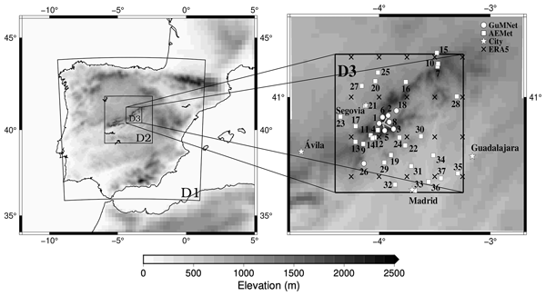
Figure 1Design of the three WRF domains in the WRF simulation and distribution of available observational sites. Left: domains D1 through D3. Right: zoom of D3 with the GuMNet (circles) and AEMET (squares) sites (numbers are listed in Table 1), ERA5 points inside D3 (crosses) and relevant cities (stars), shown for the purpose of geographical guidance. Grey shading depicts orographic altitude with the resolution of ERA5 in the outer border and the increasing resolution to the inner WRF domains. Note that grey segments are used to displace and differentiate some of the high altitude GuMNet sites.
2.1 Observations
Observational data (Table 1; Fig. 1) were obtained from two different sources in order to cover a wider altitudinal range. Eight sites belong to the Guadarrama Monitoring Network (GuMNet; Vegas-Cañas et al., 2020; García-Pereira et al., 2024b; Fernández-Castillo et al., 2025) and 29 to the Spanish Meteorological Agency (AEMET). The GuMNet facility offers the highest altitude locations while AEMET provides an extended coverage over the area and period of interest. The GuMNet sites (circles in Fig. 1) are situated in the mountain environment between 920 and 2225 Most of them are located in the southeast side of the Sierra, in the province of Madrid, except for one in the northwest side, in the province of Segovia (see stars indicating the location of nearby cities to aid geographical orientation in Fig. 1). The time coverage of these observations is limited from 2003 to 2020 in the best case and to two years of data in the case with less data (site 3). Despite its limited time span, this short-record station was intentionally included due to its high-altitude placement. The AEMET sites used in this work (squares in Fig. 1) were selected to allow for a meaningful comparison with model data and include all the available sites with good data coverage during the period of simulation, i.e. 1991 to 2020. With the AEMET sites the altitudinal range is extended to a lower bound of 607 The spatial distribution of the sites spreads mostly in a northwest to southeast direction, with lower density towards the east and northeast and to the southwest of the domain of study.
2.2 Climate simulations
The simulations used herein come from two sources: the ECMWF Reanalysis v5 (ERA5) and the Weather Research and Forecasting Model (WRF) model. The ERA5 (Hersbach et al., 2020) reanalysis (0.3° × 0.3° resolution) was used to provide the boundary conditions for the WRF model simulation (Fig. 1). Also, its simulated precipitation has been used for comparison with the WRF simulation at various resolutions and with observations to determine the added value of increasing resolution.
The WRF model (Skamarock et al., 2005; Wang et al., 2020) is a fully compressible and non hydrostatic model (with a run-time hydrostatic option) with the vertical coordinate as a terrain-following hydrostatic pressure coordinate. The grid staggering is the Arakawa C-grid and the model uses the Runge–Kutta second and third order time integration schemes, and second to sixth order advection schemes in both the horizontal and vertical dimensions. Additionally, it uses a time-split small step for acoustic and gravity-wave modes. The selected physical configuration involved parameterizations of the 4.2.2 model version, including long-wave radiation, as represented in a new version of the Rapid Radiative Transfer Model (RRTMG; Iacono et al., 2008). This considers the effects of the detailed absorption spectrum of water vapour, carbon dioxide and ozone. The short-wave radiation scheme is also based on Iacono et al. (2008). A New Tiedtke (Tiedtke, 1993; Zhang and Wang, 2017) scheme is used for the cumulus parameterization and an improved Mellor-Yamada Nakanishi and Niino Level 2.5 scheme (Nakanishi and Niino, 2006) was used to parameterise the planetary boundary layer (PBL) in the three domains. For the microphysics, the Thompson et al. (2008) scheme was implemented to describe ice, snow and graupel processes suitable for high-resolution simulations. The Noah-MP land-surface model was used to provide the heat and moisture fluxes at land points (Niu et al., 2011). The chosen surface layer model is based on Nakanishi and Niino PBL surface layer scheme (Nakanishi and Niino, 2006) and the land use and land-cover (LULC) data used to determine the physical properties of the surface was the CORINE 100 m (EEA, 2021). The topographic data for all domains were obtained from the Global Multi-resolution Terrain Elevation Data 2010 at 30 arcsec grid resolution (Danielson and Gesch, 2011). Sea surface conditions are introduced with the NOAA ° Daily Optimum Interpolation Sea Surface Temperature v2 high resolution OISST (Reynolds et al., 2007; Huang et al., 2021) and sea-ice (0.25°; approx. 25 km).
The simulation was divided into three experiments, covering two of them a time interval of one decade and the last one of eleven years: 1989–1999, 1999–2009, and 2009–2020. The first year of each experiment was spared as spin up. The complete run extends over the 1991–2020 time interval and resulted from the concatenation of each single experiment after excluding the spin up year. The long period (one year) of spin up allows for long-term processes in the soil to reach equilibrium (González-Rouco et al., 2021; Torres-Vázquez et al., 2023), with the initial conditions provided at the beginning of each experiment by ERA5.
All three experiments used an identical configuration with three nested domains without feedback, reaching a 1 km horizontal grid spacing in the innermost grid and a 1:3 ratio between the contiguous inner and outer domain resolutions, leading to three different resolutions: 9 km for the outer domain (D1) and 3 and 1 km for the inner nested domains D2 and D3, respectively. The innermost domain, D3, covers the Sierra de Guadarrama and a large area of the provinces of Madrid and Segovia (Fig. 1). The three separate WRF simulations within the D3 domain are going to be referred to as WRF1, WRF2, and WRF3 hereafter. These three correspond to the 9, 3, and 1 km resolution outputs, respectively.
(Wang et al., 2020)(Danielson and Gesch, 2011)(EEA, 2021)(Hersbach et al., 2020)(Reynolds et al., 2007; Huang et al., 2021)(Nakanishi and Niino, 2006)Nakanishi and Niino (2006)(Niu et al., 2011)Thompson et al. (2008)(Iacono et al., 2008)(Tiedtke, 1993; Zhang and Wang, 2017)Table 2Configuration used in the WRF simulation. See text and Fig. 1 for complementary information about domains and resolutions.

The model top was set to 50 hPa, following the best practices recommended by the WRF developers (Wang et al., 2019, 2020) and as in Vegas-Cañas et al. (2020) and Hahmann et al. (2020). Spectral nudging was implemented above the PBL in D1 only and an adaptive time step was used to assure the stability of the simulation (Skamarock et al., 2005). Finally, the vertical discretization was of 61 levels of the hybrid vertical coordinate. This setup information and more technical details are provided in Table 2.
(Zhang and Wang, 2017)(Kain, 2004)(Grell and Freitas, 2014)Table 3Cumulus parameterizations for WRF1, WRF2, and WRF3 for the reference simulation and for five sensitivity experiments carried out for the year 2009. All other features of the model configuration have been kept as in the reference simulation (Table 2). All simulations share the same selection for the first two domains. The last three simulations allow CPS for WRF3.
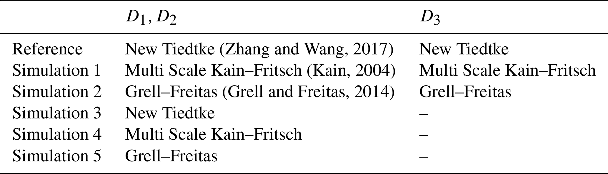
One issue that is discussed herein is the convenience of using convection-permitting schemes (Lind et al., 2020; Vergara-Temprado et al., 2020; Tomassini et al., 2023), particularly considering the focus of this work on high km-scale resolution and the fact that it targets an area of complex terrain. The 30 year long simulation presented here included the New Tiedtke (Tiedtke, 1993; Zhang and Wang, 2017) for the cumulus parameterization. The simulation had been completed before making it available for this study. In order to assess the convenience of including convection-permitting schemes, several additional experiments were performed to simulate year 2009 data during the development of this analysis, using 6 different configurations: the configuration used in the 1991–2020 simulation (Table 3) has been compared to 5 additional simulations in which cumulus parameterizations have been changed or switched off to allow for the direct simulation of convection (simulations 1–5; Table 3). All these test simulations start from the same restart file resulting from the last time step of 31 December 2008, thus sharing the same initial conditions.
The climatology of precipitation in the region is assessed herein by focusing on daily accumulated precipitation for annual and seasonal timescales: annual (January to December), spring (March, April, and May; MAM), summer (June to August; JJA), autumn (September to November; SON) and winter (December to February; DJF).
The data from the simulations were evaluated by considering the three model resolution outputs over the D3 domain (WRF1–3; Fig. 1) and also by co-locating them to the observations locations, i.e. extracting and evaluating only those grid points closest to each observational site. This will be referred to as spatial masking hereafter.
Similarly, to counteract the fact that the time span for certain observational sites is not as long as that of the simulations and to account for the potential influence of missing data, some analyses only consider in the simulations those days with available observations (temporal masking hereafter). Also, some analyses focus only on those days in the simulations in which precipitation occurs in the observations (wet masking hereafter). When simulations have been co-located and masked to the observational data availability, i.e. spatial and temporal masking, the model-observation comparison is done with the same number of data in both data sets. If masked to observational wet days, then the assessment focuses on the realism of the simulations in representing precipitation when it rains in the reality.
The relationship between precipitation and altitude has also been assessed, with the annual and seasonal means of daily accumulated precipitation for the observations and simulations being regressed against altitude.
The added value of the WRF model simulation with respect to ERA5 has been assessed using the Brier Skill Score (BSS; Von Storch and Zwiers, 1999), defined as:
where RMSE indicates the Root Mean Square Error between the simulations and the observations, calculated based on anomalies, i.e. after subtracting the averages of each of the involved time series. This avoids biases inflating RMSE estimations and allows for evaluating errors in the simulation of temporal variability. RMSEtest and RMSEref are the RMSE values for a test and a reference experiment, respectively. If the result is positive, the residuals of the test model have a smaller RMSE than the reference, so the test model outperforms the results offered by the reference. On the other hand, if BSS is negative, the reference model produces smaller residuals and thus remains better. BSS values close to 0 indicate that the test simulation performance is very similar to the performance of the reference in representing the observations.

Figure 2Total annual accumulated precipitation means for the three resolutions of WRF (9, 3, and 1 km), observations (circles) and ERA5 data (diamonds), over the D3 domain. Topographic contour lines from the 1 km resolution WRF simulation are included to highlight the complex terrain of the study area.
4.1 Climatology
Figure 2 shows the total annual accumulated precipitation mean for the three resolutions of WRF in the D3 domain, for ERA5 data (diamonds) and for the observations (circles). At all resolutions the highest precipitation values are simulated within the highest altitudes of the Sierra (Fig. 1), at the central and northeastern areas. This is especially notable in the 1 km resolution (WRF3; Fig. 2c) and also broadly consistent with ERA5 and with the observations.
It is noteworthy how the WRF simulated precipitation increases with resolution and a more realistic representation of orography, this being in principle a result of enhanced orographic ascent. In this sense, the 9 km resolution of WRF (WRF1; Fig. 2a), is a coarser representation of orography and consistently simulates a comparatively more homogeneous spatial distribution. Low altitude sites receive also the lowest observed precipitation amounts between 400–500 mm, still slightly above the values simulated by WRF1 and partially consistent with those of WRF2 and WRF3: as the resolution increases, the model simulates higher precipitation for some of those sites around the Sierra to a range of 600–800 mm (Fig. 2b and c).
The simulation at 3 km (WRF2) is reasonably consistent with the range of observations for a number of intermediate (e.g. sites 8, 10–14, 16, 19; Table 1) and high altitude (e.g. sites 1, 3, 4, 8) sites, while some sites are at odds (e.g. sites 2, 5, 9, 18), in all cases because of overestimation. This seemingly outlier behavior in the comparison with the model can be due to model deficiencies, but also due to observational limitations in temporal sampling, site selection or other causes, as it will be discussed later. Note that in all cases such discrepant sites are well under the values registered by nearby sites. Interestingly, the lowest precipitation amounts are consistently depicted by WRF2 and observations to the south east of the domain (e.g. sites 36, 37).
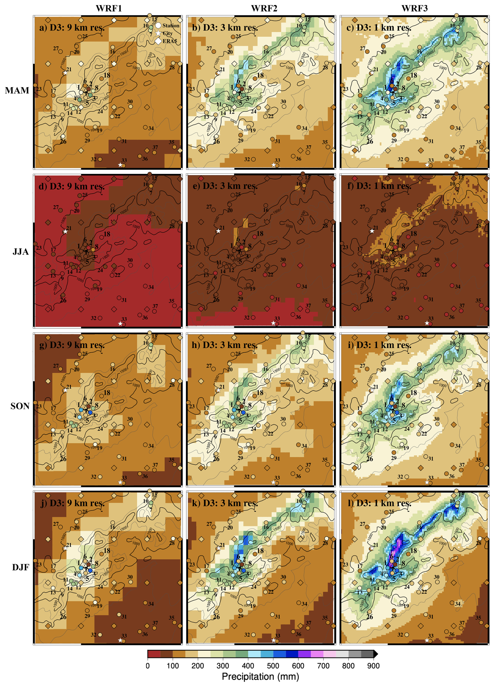
Figure 3Total seasonal accumulated precipitation mean for the three resolutions of WRF (9, 3, and 1 km), observations (circles) and ERA5 data (diamonds), over the D3 domain. Topographic contour lines from the 1 km resolution WRF simulation are included to highlight the complex terrain of the study area.
The simulation output at 1 km (WRF3) enhances precipitation in the whole domain, generating values that are above those registered at most sites. It is remarkable that the model yields values above 1500 mm at the highest altitudes, reaching 1800 mm, where no observations are available. Although those values are very likely overstated, since the simulation overestimates almost elsewhere, it is interesting to note that in the highest areas, where the heaviest rainfall could occur, there are no observational sites that allow comparisons with the simulation. Overall, WRF2 seems to produce a climatology at least as consistent with observations as WRF3. Seasonal climatology is shown in Fig. 3 (rows) for the three WRF resolutions (columns), ERA5 and observations. Winter registers the highest precipitations in the Sierra de Guadarrama (Fig. 3j–l), but not in the piedmonts and the valleys, where the maxima occurs in autumn and spring (Fig. 3a–c and g–i, respectively). Summer is by far the driest season, registering precipitations below 50 mm in Madrid and nearby sites (Fig. 3d–f). In fact, these low levels are consistent with WRF1 in all the southern half of the domain. WRF2 and WRF3 simulate also low values, although slightly above that level. Nevertheless, at the high altitude and northeastern sites, WRF2 and particularly WRF3 represent better the slight increases of average summer precipitation above 100 mm. WRF1 tends to underestimate precipitation at all seasons, although in spring and autumn it yields a better model-data agreement at some low altitude sites. On the other hand, WRF2 tends to be consistent with observations at low and intermediate sites and somewhat underestimate at high altitude, particularly in winter. For the highest altitudes, WRF3 seems to produce more consistent values. The gradient of precipitation with height is remarkable within the top few grid points in WRF3. This is consistent with reports from Morán-Tejeda et al. (2021) and with the high values of some sites in winter. Thus, although the realism of the sharp increase of high altitude precipitation remains uncertain and could be a feature of the model, it is consistent with the behavior of the limited observational information. Better observational sampling could help as well to ascertain if this behavior is realistic or if the model overstates the role of altitude.
Regarding ERA5, precipitation values are generally in better agreement to observations within the lowlands to the northwest and southeast of the domain. In the southwest-northeast direction ERA5 values are slightly larger but strongly underestimate site data over the area of the Sierra de Guadarrama. Interestingly, the largest ERA5 precipitation values are in the range of 200–250 mm and take place in spring and autumn, whereas for WRF the largest values are clearly attained in winter for all resolutions. It is difficult to ascertain whether this is the case in reality from the available sites, at high altitudes.

Figure 4Observed and simulated precipitation occurrence described by the percentage of days with appreciable (> 0.2 mm) precipitation for annual and seasonal data. For the annual analysis, each station in the x-axis includes 5 different bars corresponding to the observations and the ERA5 and WRF simulations; the latter including the output for the three model resolutions (see labels and colours). The four panels at the bottom represent the seasonal cases and include the observations and only the WRF3 simulation output. Orange solid boxes represent the percentage of observed days per year with appreciable precipitation. Solid boxes in the simulations represent also the appreciable precipitation, but considering only the days with appreciable rainfall in observations (masking to wet days). Hatched boxes represent the percentage of appreciable precipitation occurrence if the days with available observation, either dry or wet, are considered (masking to data existence). Hollow boxes indicate the occurrence of appreciable rainfall in the simulations during the time, i.e. the number of years, in which the station is working (no temporal masking). Stations in the horizontal axis are labeled according to Table 1 and ordered by altitude.
4.2 Precipitation distribution
To assess how the models represent the occurrence of precipitation, Fig. 4 shows the percentage of days per year with appreciable (> 0.2 mm) precipitation at each site. The occurrence of wet days has been compared in three different ways: by considering the complete availability of observational and simulated data, which for the observations is the time during which a site has been in operation; by considering only days with availability of observational data (temporal masking); and by considering only days with appreciable precipitation in observations (wet masking). For the three assessments, simulation data has been co-located (spatially masked), to extract the closest simulation grid point to each observational site (see Sect. 3).
At low altitude sites, like those situated in the city of Madrid (33/MRT; Table 1) and nearby stations, the observed percentage of days with appreciable precipitation (orange boxes; Fig. 4) is around 20 %. This percentage tends to increase with altitude reaching maxima above 40 % at sites 3 and 8 (HYS and CBM), located above 2000 and 1500 , respectively. In fact, at the highest altitudes, there are notorious differences between nearby sites, especially between sites 2 and 3 (ZBL and HYS), probably because of missing data (hatched and hollow boxes in Fig. 4). This is most pronounced in the case of site 2, particularly for winter (DJF; Fig. 4). This could be due to data sampling problems caused by heavy snowfall or from accessibility and maintenance issues on sites during winter.
Summer is the season with the smallest percentages of wet days (JJA; Fig. 4) with wet days percentages at most sites between 10 % and 20 %. For the other seasons, comparable values are attained and are in the range of those for the annual case (between 30 % and 40 %). For all seasons, progressive precipitation increases with altitude are apparent. The distinct behavior of some higher altitude sites showing comparatively smaller percentages (e.g. 2/ZBL, 5/CTS, 9/ADL, 11/FNF) is also reproduced at all seasons.
The wet masking in simulations explains how well the simulations describe rainfall days in reality. Filled boxes in Fig. 4 represent this analysis and show that the three resolutions of WRF simulations and the reanalysis provide similar results. When precipitation occurs, ERA5 and WRF also simulate wet days, with wet day occurrence being underestimated by less than 5 %. No model or WRF resolution variant outperforms the others.
When simulations are masked to data existence (hatched boxes in Fig. 4), the reanalysis and WRF, regardless of the resolution, generate days with appreciable precipitation that do not occur in reality. The number of days per year with appreciable precipitation is overestimated (ratio of hatched and solid boxes) by a factor of about 1.5, which is higher for summer (JJA; Fig. 4), when simulations produce more than twice as many wet days as recorded in observations. It is also worth noting that the season with more wet days simulated by WRF3 is spring (MAM; Fig. 4), regardless of altitude, a feature that is produced by all WRF resolutions and ERA5 (not shown). The overestimation of wet days is prone to produce precipitation totals that are higher than those observed.
The non-masked simulations (hollow boxes in Fig. 4) show much more dependence with altitude and tend to homogenize differences between close sites. This reinforces the idea that the differences between nearby stations concerning observational records and masked assessments could be because of missing data. In fact, the biggest differences between hollow and hatched boxes occur for stations with short data series, such as sites 2/DHS and 1/ZBL (Table 1). The percentage of simulated wet days per year during the time span of operation of the station is ca. 50 % for altitudes above site 18/ALM (1100 ). Below that level, it decreases progressively down to site 32/MJD (725 ), below which it remains fairly constant at 30 % of rainy days per year. All of these lower stations are located in the southeast of the D3 domain (Fig. 1), near the city of Madrid (see also Sect. 4.1).
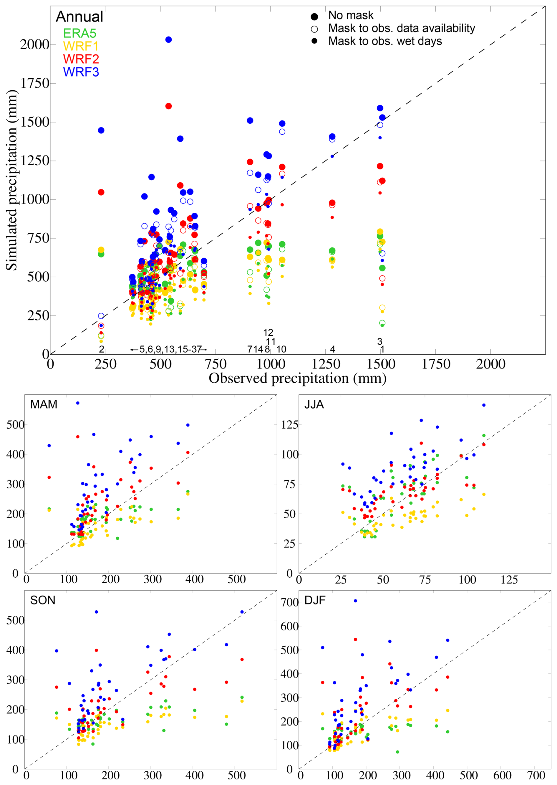
Figure 5Observed and simulated (ERA5 and WRF) mean of annual and seasonal accumulated precipitation within the D3 domain. For the annual case, big coloured circles represent appreciable precipitation during the time of data availability for each site; hollow circles represent data if the days with available observation, either dry or wet, are considered (temporal masking) and little coloured circles represent data that consider only the days with appreciable rainfall in observations (wet masking). For the seasonal panels, only the results of unmasked data are shown. The numbers labeled in the x axes of the top panel identify the corresponding stations in Table 1. The dashed black line represents the range of equal values in observations and simulations.
The observed and simulated precipitation totals are compared in Fig. 5 in dispersion diagrams for mean annual and seasonal accumulated precipitation values. The closer the points are to the diagonal line, the more accurate are the simulated precipitation totals. The simulated data have been co-located to observational sites (spatial masking) and both temporally masked and unmasked simulated data have been evaluated for the annual case. Seasonally, only the non-masked data have been represented.
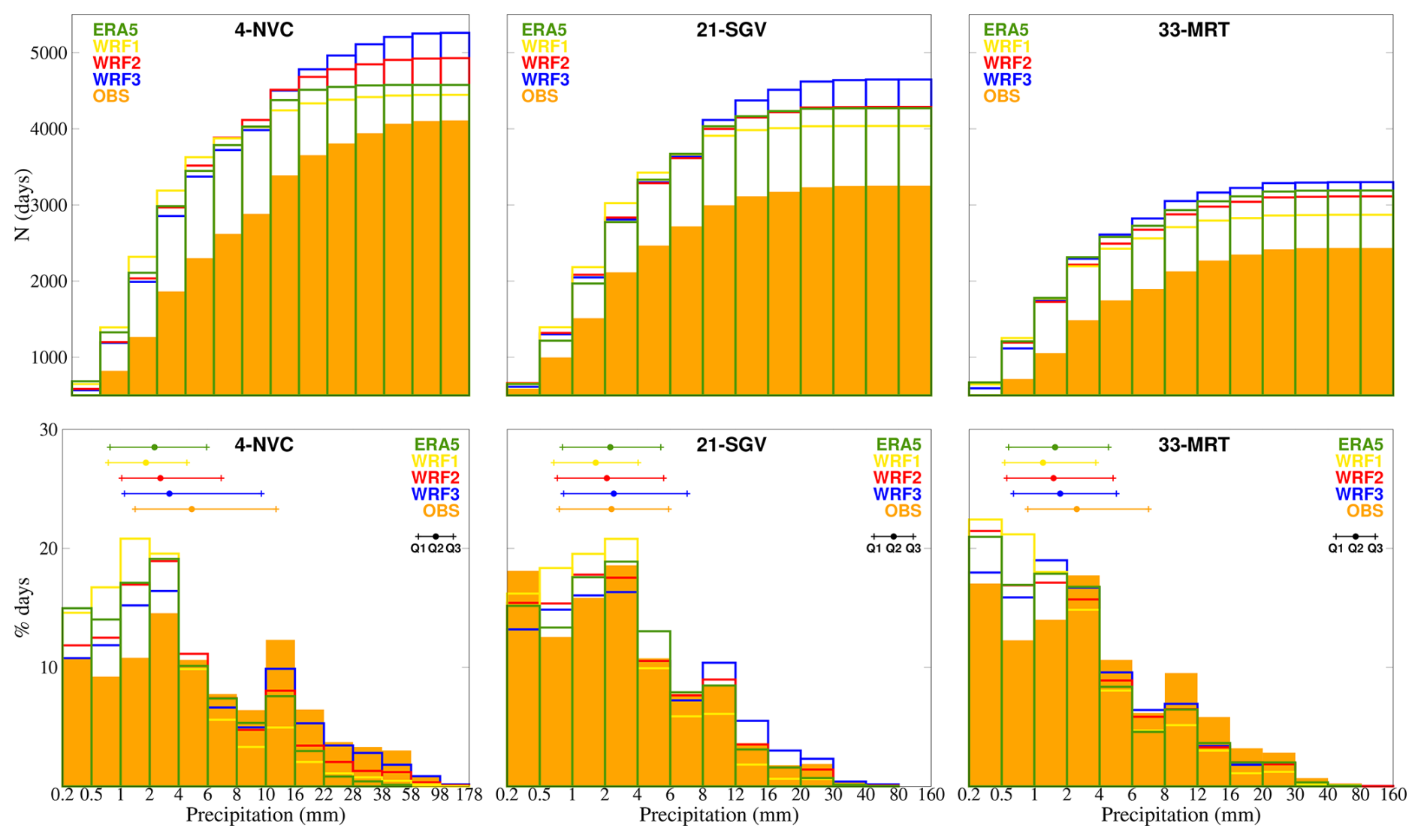
Figure 6Accumulated absolute and relative distributions of daily precipitation. Top: histograms of daily precipitation in accumulated absolute frequencies, for sites 4/NVC, 21/SGV, and 33/MRT. Bottom: histograms of daily precipitation relative frequencies at the same sites. See legend for colours identifying ERA5, WRF and observations. At the bottom plots, the coloured segments depict the position of the Q1, Q2 (median) and Q3 quartiles in ERA5, WRF and observational samples. Data have been temporally masked to produce model and observational estimates from synchronized samples of equal size.
In terms of the total accumulated precipitation, WRF3 tends to overestimate for all seasons and the annual case, except for some sites during autumn and winter (SON and DJF; Fig. 5) with precipitation in the range of 100–150 mm. WRF1 and ERA5 underestimate for sites with precipitation totals above 700 mm, and to a greater extent for the higher accumulations. As for the lower resolutions, WRF1 outperforms ERA5 slightly in DJF, but does not improve in general the performance of the reanalysis, with ERA5 actually producing better results in spring and autumn (MAM and SON; Fig. 5). WRF2 tends to underestimate slightly the largest precipitation totals in the annual case, but overall it is closer to observations than WRF3 for all seasons (solid circles). For most sites, the annual differences between the hollow and solid circles, i.e. temporal masking or no masking, are small, but for some sites (e.g. 2/ZBL) they are noteworthy, thereby indicating the effect of missing data in the totals and that the observational sampling is likely not capturing well precipitation occurrence, as in Fig. 4. For the case of the wet masking (small circles), it becomes evident that the WRF3 estimates are much closer to observations. This occurs when restricting the precipitation counting of the simulations to the observational wet days. Since WRF produces more wet days than observations (Fig. 4), total precipitation is overestimated. Seasonally, wet masking WRF3 reduces this overestimation considerably and its values are fairly close to the diagonal line. The other resolutions tend to underestimate the observations, except for WRF2 in winter (not shown).
As shown by the station code identifiers (Table 1) alongside the horizontal bottom axis of Fig. 5 in the annual case, typically the higher accumulations, both observed and simulated, correspond to the highest altitudes, except for site 2/ZBL (Table 1). This site behaves as an outlier, likely because of the high proportion of missing data as discussed earlier.
The distribution of probability of precipitation totals into ranges of daily accumulated values are discussed with Fig. 6 for the case of threes sites: histograms of relative and accumulated frequencies of daily appreciable precipitation for the observations and for temporally masked simulations are shown for Navacerrada, Segovia, and Madrid Retiro (sites 4/NVC, 21/SGV, 33/MRT; Table 1). These three stations have been selected because they cover a long time period, a wide altitudinal range and because of their geographical position: 21/SGV at the west side of the Sierra; 4/NVC, located at the heart of the Sierra; and 33/MRT, at the east side, in the city of Madrid, and at a relatively lower altitude.

Figure 7Relative distributions (boxplots) of appreciable precipitation in simulations and observations. Top: boxplots of the three resolutions of WRF, ERA5 and the observations at each station. WRF and ERA5 data has been co-located for each observational site, as well as temporally masked to data existence. On each boxplot: the bottom whisker represents the 10th percentile; the lowest part of the box shows the first quartile; the highest part of the box shows the third quartile; the top whisker shows 90th percentile and the lines above show the 99th percentile (note the different axis). The median is represented with a white dot inside the box. Bottom: analogous representation for the seasonal assessment focusing on WRF2, WRF3 and the observations. Stations in the horizontal axis are labeled according to Table 1 and ordered by altitude.
These histograms of accumulated precipitation agree with Fig. 4 in showing that there is more occurrence of wet days at the higher altitude sites and also in the model simulations than in observations. The 1 km resolution of WRF, WRF3, is the one that overestimates these days the most, especially for sites 4/NVC and 21/SGV. For 33/MRT the frequencies of WRF3 are comparable to ERA5 reanalysis. The total number of wet days in the simulations that did not occur in reality can be on the order of 1000 (approximately 30 d yr−1) for sites 4/NVC and 21/SGV and a bit smaller for 23/MRT (see differences between the simulated and observed absolute accumulated frequencies at the last class interval). Notice that the overestimation grows from the first classes and after ca. 10 mm it remains fairly constant for WRF1 and increases slightly for the other model outputs. This can be better understood with the relative probability plots (Fig. 6; bottom row), where normalized frequencies are depicted for observations and simulations in order to better describe the class intervals that receive most precipitation occurrence.
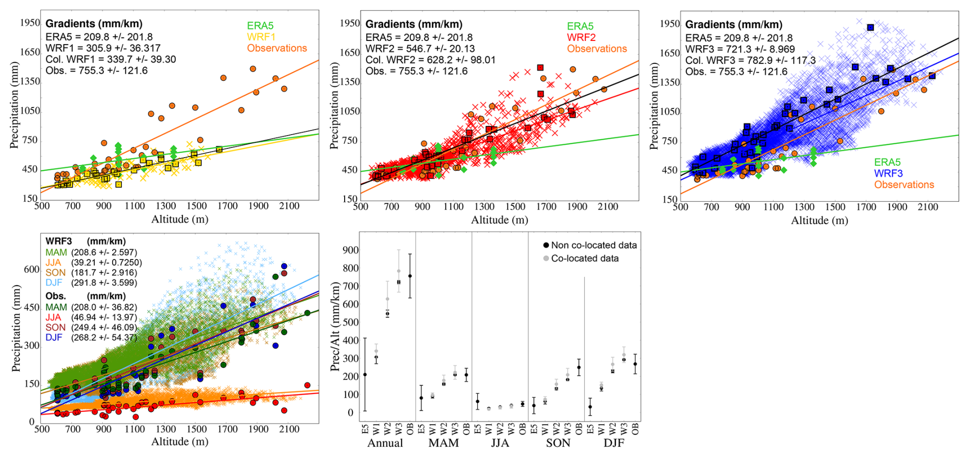
Figure 8Description of precipitation changes with altitude. Top: altitudinal distribution of observed and simulated mean of annual accumulated precipitation for WRF, ERA5 (diamonds) and observations (circles). WRF data is represented with crosses and observations co-located WRF data with squares. The results of several linear fits of precipitation totals and altitudes are shown for observations, ERA5 and WRF complete outputs (colours) and co-located data (black lines). Months with more than 20 % missing data have been excluded from the analysis. Bottom left: altitudinal distribution of observed and simulated mean of seasonal accumulated precipitation of WRF3 (crosses; including all model grid points in D3) and observations (circles): MAM (green), JJA (orange), SON (brown), and DJF (blue). Bottom right: representation of the ratios of precipitation (mm) and altitude (km) for ERA5, WRF and observations for the annual and seasonal cases. Grey symbols correspond to co-located WRF data and black to non co-located WRF data.
The segments included in these plots show the range of values for the first to third quartile (Q1 and Q3 in the legend; Fig. 6) in observations, WRF and ERA5. 25 % of wet days occur for very low precipitation amounts of about 1 mm, 50 % are in the 2–6 mm and 75 % below 10 mm, so about 75 % of wet days distribute over rather small daily precipitation amounts, between 0.2 and about 10 mm, this being also the range over which the simulations overestimate precipitation occurrence.
Overall, the shape of the distribution is well reproduced by the simulations. In general, WRF1 tends to overstate small precipitation events in the three example sites, whereas ERA5 does it at sites 33/MRT and 4/NVC and produces a more accurate distribution at site 21/SGV. WRF3 shows a better performance than WRF1 at all sites, reducing percentages at the lowest classes and increasing them at the highest, where the other model outputs tend to underestimate the observations, probably as a result of orographic precipitation enhancement.
The segments indicating the positions of the quartiles show broadly very similar ranges for the observations and the simulations. For the site at the highest altitude, the WRF3 range is the closest to the observations.
The previous analysis is extended to all sites in Fig. 7. Box and whiskers plots are shown for observations at each site and all model simulations for the annual case. Additionally, for all seasons, the assessment shows observations, WRF2 and WRF3, specifically. Whiskers range between the 10th and 90th percentiles while boxes illustrate the 25 %–75 % range, with the median inside marked by a white dot. Additionally, extreme data are depicted by showing the 99th percentile in the top lines (note the different axis for these in Fig. 7). For many sites the simulations tend to underestimate the observed annual statistics (e.g. sites 8, 11, 12, 14, 19, 20, 23, 24, 26, 28, 30, 31, 32, 35), while for the others simulations, particularly WRF3, broadly agree with the range of variability of observations (e.g. sites 3, 6, 9, 10, 29); for a number of sites WRF2 performs as well as or better than WRF3 (e.g. sites 13, 17, 18). The range of variability tends to be higher for the most elevated stations and the relative changes from site to site are also captured by the simulations. For the lower altitude sites all simulations produce very similar distributions, but for the higher, the ranges differ. Typically ERA5 and WRF1 underestimate the most, while WRF2 and WRF3 are closer to the observational ranges, as depicted by the box and whiskers plots. WRF1, for those sites, tends to show the worse results, worse than ERA5, while WRF3 tends to show the best. Therefore, for the low altitude sites there is little improvement with the resolution enhancement, while for higher altitudes the added value of increased resolution is higher. This is even clearer for the 99th percentile: for all altitudes ERA5 and WRF1 tend to underestimate extreme values and particularly for the higher altitude sites; however WRF2 and WRF3 match the range of observed values, slightly overestimating at some low altitudes sites, while for higher altitudes, both high resolution outputs, and particularly WRF3, are the closest to observations. The seasonal analysis shows very similar results for spring, autumn and winter (notice the different ranges in the distribution), with winter being the season with the largest daily precipitation values and largest contrast between low and high altitude sites.

Figure 9Brier Skill Score for annual accumulated co-located and masked data of appreciable precipitation for the three resolutions of WRF (9, 3, and 1 km) in comparison with ERA5.
The summer statistics are noteworthy as they show several distinct features: the contrast between low and high altitude sites is minor, in comparison to other seasons, in observations and absent in WRF2 and WRF3; and the WRF2 and WRF3 simulations systematically underestimate precipitation at virtually all sites, the underestimation being notable for the third quartile and the 90th and 99th percentiles. This is suggestive of the dominant character of convection and of problems in adequately simulating convection with the current configuration of the model.
The comparison between the altitudinal distribution of precipitation for the different WRF configurations and for the observations is intended to characterize the importance that each resolution attaches to the influence of orography on precipitation. Figure 8 shows that there is a positive correlation between precipitation and altitude, being more intense for the higher resolutions. This representation is somewhat simplistic as it does not consider subregions or orientations of orography to the different directions of the atmospheric flows. Nevertheless, it allows for a first order comparison of precipitation rates with altitude in observations and simulations. Total accumulated annual precipitation means for observational data increase at a rate of 755.3 mm km−1. The coarser representation of orography at lower resolutions causes that neither ERA5 (209.8 mm km−1) nor WRF1 (305.9 mm km−1) are able to simulate this dependency well. WRF2 and WRF3 reach ratios of 546.7 and 721.3 mm km−1, respectively. When evaluating only the spatially masked grid points of WRF, observations and simulations yield closer gradient values, corresponding to 339.7, 628.2 and 782.9 mm km−1 for co-located WRF1, WRF2 and WRF3, respectively.
The bottom left panel of Fig. 8 shows the seasonal altitudinal distribution of WRF3 data and observations. WRF3 shows a higher gradient value than observations for winter, (DJF; Fig. 8), but less for autumn (SON; Fig. 8). Spring and summer (MAM and JJA; Fig. 8) report similar values. This indicates that winter orographic ascent is the dominant influence of altitude. The summertime contribution of altitude to convection is more evident in this figure than in Figs. 5 and 7, but relatively minor in comparison to other seasons.
The bottom right panel of Fig. 8 allows to effectively quantify the increasing dependence of precipitation on altitude with resolution. The role of resolution in correctly representing the orography when simulating the precipitation is remarkable at all seasons, and particularly in winter (DJF; bottom right panel, Fig. 8), when WRF3 simulates a gradient 6 times larger than ERA5; even in summer, the progressively increasing resolution of the WRF outputs produces more realistic precipitation rates with altitude than ERA5. Co-located estimates produce, in all seasons but summer, higher values. WRF3 estimates are then on the higher end of the observations for winter and spring, with WRF2 producing more accurate estimates, especially for winter. In autumn, WRF3 is the closest to observations after considering only the co-located grid points. For the summer, the differences are negligible. The 95 % confidence intervals for the regression coefficients are very small for the non co-located simulations due to the large number of data involved in the estimation. Co-located data and observations show similar uncertainty ranges in their estimates of the annual and seasonal cases, except for summer (JJA; bottom right panel, Fig. 8), when values are very close to zero, this being the result of the low spatial variability in the simulation of summer precipitation (e.g. Fig. 7).

Figure 10Brier Skill Score for seasonal accumulated co-located and masked data of the appreciable precipitation for the three resolutions of WRF (9, 3, and 1 km) in comparison with ERA5.
Finally, the added value of the WRF model simulation, in its three resolutions, with respect to ERA5 has been assessed making use of BSS for the annual case (Fig. 9) and for the seasonal cases (Fig. 10). This allows to assess the relative improvements of increasing physical detail not only in the properties of the simulated distribution in comparison to observations, but also in the actual errors (RMSE) of the simulated WRF data with respect to observations and in comparison to those of the ERA5 simulations as a reference. The more positive the values of BSS, the better the simulation represents observations with respect to the reanalysis; and the more negative, the lower the added value of WRF on ERA5 (Sect. 3).
The comparison of annual values between the output of the three resolutions and ERA5 (Fig. 9) yields positive BSS values for most sites, so that the performance of the WRF improves, in general, that of ERA5 in representing the observations. The statistics obtained for WRF2 at 3 km resolution are visibly the best, improving BSS values at high altitude sites relative to WRF1. WRF3 performs better in general than ERA5 and WRF1, but it does not improve BSS relative to WRF2, producing values that except for some sites (e.g. site 3) are similar or lower to those of WRF2. Some of them display even negative values (e.g. sites 6, 10 or 31), thus indicating loss of performance relative to ERA5.
Figure 10 expands the information of Fig. 9 to all seasons. The seasons that show most improvement in the reduction of residual variance are spring and autumn, particularly for WRF1 and WRF2, with most high altitude sites and sites at the north and southern plains showing reductions of error relative to ERA5. However, concerning WRF3, some sites (e.g. sites 6, 7, 10, 16, 31, 34) do not show improvements. Also, interestingly, increasing resolution does not necessarily improve residual variance in winter and at a few sites (e.g. sites 8, 13, 16, 17, 21, 26, 29, 34) performance worsens. Summer is the season rendering worse model results.
4.3 Discussion
From the previous analysis we learn that increasing model resolution can therefore improve model biases in the representation of the annual and seasonal distribution of precipitation at higher altitude sites, but not necessarily error variance when assessing model-data residuals. Model-data errors can show notable local improvements for some sites (mostly high altitude) and seasons (mostly winter) while deteriorating at other sites and seasons, and also with increasing resolution (Figs. 9 and 10). There are at least two factors that can contribute to this behavior. One is the sensitivity to the metrics that are used to quantify the performance of the model-observation errors. As designed in Figs. 9 and 10, the closest grid point to the observational sites is selected. When increasing resolution this imposes important requirements to the analysis as, particularly in the case of convective precipitation, local systems can be realistically simulated and yet, not generate precipitation necessarily at the closest grid point to a given observational site. This can be recalled as type of representation error (e.g. Jiménez et al., 2013a; Van der Plas et al., 2017). Therefore, more flexible approaches that allow for introducing some uncertainty in the evaluation of the spatial skill of model in simulating convective precipitation seem advisable. The other issue that can contribute to the performance of the model at kilometer scale resolutions is the configuration of the simulation and, specifically, the selection of a given convection parameterization or its exclusion in convection-permitting schemes (CPS, Belušić et al., 2020; Lind et al., 2020; Solano-Farias et al., 2024). The long simulation included herein adopts a New Tiedtke scheme (Tiedtke, 1993; Zhang and Wang, 2017, Table 2) as the cumulus parameterization for the three model resolutions. This may be arguably appropriate for resolutions beyond 9 km, a range which this parameterization has been found to produce realistic results (Bi-Yun and Xun-Qiang, 2019; Bopape et al., 2021; Wang, 2022; Bello-Millán et al., 2024), however, at higher resolutions like 3 or 1 km other parameterizations or CPS approaches may be more adequate (Prein et al., 2015; Ban et al., 2021; Solano-Farias et al., 2024)
In order to better understand the sensitivity to using different convection parameterizations or adopting CPS approaches, various sensitivity tests have been carried out changing the cumulus parameterization for year 2009. The reference simulation (see Table 3 for any of the simulations discussed below), which corresponds to the WRF configuration used in this work, uses the New Tiedtke parameterization (Tiedtke, 1993; Zhang and Wang, 2017). Simulation 3 has the New Tiedtke scheme activated for WRF1 and WRF2, but lets the model resolve convection itself at the 1 km resolution, so that no cumulus parameterization is considered for the highest resolution (WRF3) following a CPS approach. Simulations 1 and 4 consider Multi Scale Kain–Fritsch (MSKF; Kain, 2004) convective parameterization: simulation 1, for the three resolutions and simulation 4, only in WRF1 and WRF2 allowing for CPS in WRF3. Finally, simulations 2 and 5 use Grell–Freitas cumulus parameterization: simulation 2 with the cumulus scheme activated for the three resolutions and simulation 5 with cumulus parameterization activated in WRF1 and WRF2 and no cumulus parameterization activated for WRF3. Note that this selection of configurations is somewhat arbitrary and accommodated to test a couple of specific changes in cumulus parameterizations. Also, CPS approaches could have been implemented already for the 3 km resolutions. Nevertheless, it allows for briefly inspecting with a few relatively short simulations of one year, the potential of changing how the simulation of convection is affected. Additional simulations were performed changing the microphysics parameterization to National Severe Storms Laboratory double-moment parameterization (NSSL2; Mansell et al., 2010), but rendered non-significant results and are not reported here.

Figure 11Comparison between observed and simulated annual accumulated precipitations by WRF and ERA5 within the D3 domain for configurations of WRF involving different concerning cumulus parameterizations and CPS approaches. Symbol convention follows that of Fig. 5.
Figure 11 shows, in the same fashion as in Fig. 5, the dispersion diagrams between observed and simulated annual accumulated precipitation by WRF and ERA5 for the different schemes described in Table 3 within the D3 domain. The inclusion in simulation 3 of a CPS approach in D3 with respect to having New Tiedtke scheme in the three domains introduces notable differences, with clear underestimations for sites with precipitation total between 250 and 400 mm. For the few sites above this level, WRF3 simulated precipitation is in general more in the range of observations. Simulation 1 and simulation 2, including the MSKF and Grell-Greitas (Table 3) parameterizations in the three domains do seem to improve results with respect to the reference simulation, producing precipitation totals that are more in the range of observations. Differences between simulation 1 and simulation 2 are negligible and, interestingly enough, for both cases including CPS in D3 does not produce noticeable differences, consistent with Solano-Farias et al. (2024).
This work has evaluated the variability of precipitation in the Sierra de Guadarrama and nearby lowlands, reaching the cities of Madrid, Segovia and adjacent territories during the period 1991–2020. For this purpose, daily accumulated precipitation data from 37 stations, with altitudes ranging from 600 to 2200 ; as well as a simulation with the WRF model configured with 3 different domains at resolutions of 9, 3, and 1 km have been assessed. The ERA5 reanalysis, used as boundary conditions for the WRF simulation, has been also used for comparison as a means of benchmark.
Comparison of accumulated annual precipitation means of the different data sets shows that the rainiest areas of the spatial domain are those located at higher altitudes, with a few sites collecting more than 1000 mm yr−1.
For the WRF simulations the maximum precipitation increases with resolution from maximum values of about 750 mm yr−1 for 9 km to values above 1800 mm yr−1 over the highest grid points at 1 km resolution. Such values are likely overestimated if we take into account the fact that the model tends to overestimate at 1 km resolution at the grid points co-located to the observational sites. Nevertheless, it is difficult to ascertain the level of maximum precipitation at the top of the mountain range as those areas are not observationally sampled. From the available data, it is also hard to determine which one is the wettest season, but the model simulations clearly suggest that the largest precipitation amounts occur in winter.
Precipitation occurrence shows the best model-data agreement when considering only observational wet days, so that the model accurately simulates the days on which it actually rains. On the contrary, both ERA5 and WRF simulate more wet days than they occur in reality, regardless of the resolution. These extra wet days bring commonly very little rainfall, but they do affect the simulated precipitation totals, annually and seasonally. In this sense, the most impacted resolution is WRF3 (1 km resolution of WRF), which overestimates precipitation at almost all sites. However, as well as WRF2 (3 km resolution of WRF), it adds value in comparison to the lower resolutions at the highest altitudes, where ERA5 and WRF1 (9 km resolution of WRF) underestimate observations. Higher resolutions of WRF, which resolve orography more accurately, attach more importance to the influence of altitude on precipitation, so that they provide the most precise simulations of precipitation distribution for the highest altitudes. In spite of the overestimation of daily precipitation with increasing resolution, the distribution of simulated precipitation generally improves with increasing resolution for winter, spring, and autumn, specifically for extreme values. This is when high resolution provides the greatest value. Regardless of this, still the width of the relatively narrow precipitation distribution, and specifically extremes are underestimated even at the 1 km resolution for the summer season.
Altitude influences precipitation and the observational rates of increase of annual precipitation are of 755.3 ± 121.1 mm km−1 best matched, although slightly overestimated, by the 1 km resolution output (782.9 ± 117.3 mm km−1). In descending order, the largest seasonal rates occur in winter, autumn, and spring in observations and are best matched by the 3 km (spring and winter) and the 1 km resolution output (autumn); the latter slightly overestimating in winter and spring.
Increasing model resolution improves some model biases in the representation of the annual and seasonal distribution of precipitation at higher altitude sites, but not necessarily the variance of model versus observation errors. Residuals show notable local improvements at a number of sites, both at high and low altitudes; this is clear in winter, but also noticeable in spring and autumn. Nevertheless, the analysis of model-data residuals should also be targeted with more adequate metrics that consider the possibility that allows for the simulation of convective precipitation in a wider spatial domain rather than the nearest grid points.
Several sensitivity tests have been performed by changing the cumulus parameterization and by allowing CPS at the 1 km resolution. The results of the tests are promising and suggest that the New Tiedtke parameterization used in the reference configuration improves if CPS is allowed in the innest domain. Using the MSKF and Grell Freitas schemes instead of the New Tiedtke also seems to provide improvements at the km scale, although including CPS in the innest domain did not produce visible reductions in biases. More specific tests would be advisable to develop a more thorough analysis, likely including other parameterization tests.
WRF source code used in this work is available at https://doi.org/10.5281/zenodo.19663814 (Navarro-Montesinos et al., 2026). Observational, simulated, and reanalysis data used in this work are available at https://doi.org//10.5281/zenodo.19712267 (Greciano-Zamorano et al., 2026).
EGZ and JFGR planned the manuscript objectives and structured and wrote the first draft. JNM and EGB performed the simulations. ERC, ERG, CVC, and FGP helped with the initial compilation of the data and some observational analysis. All authors contributed to shaping the experiment design and evaluation in different meetings. All authors contributed to improving the manuscript text until submission.
The contact author has declared that none of the authors has any competing interests.
Publisher's note: Copernicus Publications remains neutral with regard to jurisdictional claims made in the text, published maps, institutional affiliations, or any other geographical representation in this paper. The authors bear the ultimate responsibility for providing appropriate place names. Views expressed in the text are those of the authors and do not necessarily reflect the views of the publisher.
This work has been developed under the frame of the Climate Research Initiative for Iberian Mountain Areas (CIMAs). We would like to thank the Guadarrama Monitoring Network (GuMNet; https://www.ucm.es/gumnet, last access: 5 October 2026) as well as the Spanish Meteorological Agency (AEMET; https://www.aemet.es, last access: 5 October 2026) for providing observational data. We acknowledge the support from the Polar and Geosciences Scientific Networks in the Consejo Superior de Investigaciones Científicas (CSIC), Spain. We thank NCAR and ECMWF for making the WRF model code and ERA5 outputs available. The authors acknowledge the Centro Extremeño de Tecnologías Avanzadas (CETA-CIEMAT) for providing access to its computational resources and technical infrastructure. We would also like to thank the SmileAtYou (PID2022-139719OB-I00) project.
The article processing charges for this open-access publication were covered in part by the CSIC Open Access Publication Support Initiative through its Unit of Information Resources for Research (URICI).
This paper was edited by Juan Antonio Añel and reviewed by two anonymous referees.
Adler, C., Wester, P., Bhatt, I., Huggel, C., Insarov, G., Morecroft, M., Muccione, V., and Prakash, A.: Cross-Chapter Paper 5: Mountains, in: Climate Change 2022: Impacts, Adaptation and Vulnerability. Contribution of Working Group II to the Sixth Assessment Report of the Intergovernmental Panel on Climate Change, edited by: Pörtner, H.-O., Roberts, D. C., Tignor, M., Poloczanska, E. S., Mintenbeck, K., Alegría, A., Craig, M., Langsdorf, S., Löschke, S., Möller, V., Okem, A., and Rama, B., Cambridge University Press, Cambridge, UK and New York, NY, USA, 2273–2318, https://doi.org/10.1017/9781009325844.022, 2022. a
AEMET and IPMA: Atlas climático ibérico: temperatura del aire y precipitación (1971–2000), 1st Edn., Agencia Estatal de Meteorología, Instituto Português do Mar e da Atmosfera, ISBN 978-84-7837-079-5, 2011. a
Ali, E., Cramer, W., Carnicer, J., Georgopoulou, E., Hilmi, N. J. M., Le Cozannet, G., and Lionello, P.: Cross-Chapter Paper 4: Mediterranean Region, in: Climate Change 2022: Impacts, Adaptation and Vulnerability. Contribution of Working Group II to the Sixth Assessment Report of the Intergovernmental Panel on Climate Change, edited by: Pörtner, H.-O., Roberts, D. C., Tignor, M., Poloczanska, E. S., Mintenbeck, K., Alegría, A., Craig, M., Langsdorf, S., Löschke, S., Möller, V., Okem, A., and Rama, B., Cambridge University Press, Cambridge, UK and New York, NY, USA, 2233–2272, https://doi.org/10.1017/9781009325844.021, 2022. a
Ban, N., Caillaud, C., Coppola, E., Pichelli, E., Sobolowski, S., Adinolfi, M., Ahrens, B., Alias, A., Anders, I., Bastin, S., Belušić, D., Berthou, S., Brisson, E., Cardoso, R. M., Chan, S. C., Christensen, O. B., Fernández, J., Fumière, J., Gorodetskaya, I. V., Giorgi, F., Hodnebrog, Ø., Kerschner, M., Kjellström, E., Lenderink, G., Lung, T., and Milovac, J.: The first multi-model ensemble of regional climate simulations at kilometer-scale resolution, part I: evaluation of precipitation, Clim. Dynam., 57, 275–302, https://doi.org/10.1007/S00382-021-05708-W, 2021. a
Barry, R.: Mountain weather and climate, 3rd Edn., Cambridge University Press, New York, USA, ISBN 978-0-521-68158-2, 2008. a
Bello-Millán, F. J., Palacios, J., Gutierrez-Castillo, P., and Parras, L.: Simulations of a tornadic supercell event in the south of Spain: Sensitivity to initial and boundary conditions and microphysics parameterizations, Atmos. Res., 300, https://doi.org/10.1016/j.atmosres.2024.107262, 2024. a
Belušić, D., de Vries, H., Dobler, A., Landgren, O., Lind, P., Lindstedt, D., Pedersen, R. A., Sánchez-Perrino, J. C., Toivonen, E., van Ulft, B., Wang, F., Andrae, U., Batrak, Y., Kjellström, E., Lenderink, G., Nikulin, G., Pietikäinen, J.-P., Rodríguez-Camino, E., Samuelsson, P., van Meijgaard, E., and Wu, M.: HCLIM38: a flexible regional climate model applicable for different climate zones from coarse to convection-permitting scales, Geosci. Model Dev., 13, 1311–1333, https://doi.org/10.5194/gmd-13-1311-2020, 2020. a
Bi-Yun, S. and Xun-Qiang, B.: Validation for a tropical belt version of WRF: sensitivity tests on radiation and cumulus convection parameterizations, Atmos. Sci. Lett., 12, 192–200, https://doi.org/10.1080/16742834.2019.1590118, 2019. a
Bindoff, N., Stott, P., AchutaRao, K., Allen, M., Gillett, N., Gutzler, D., Hansingo, K., Hegerl, G., Hu, Y., Jain, S., Mokhov, I., Overland, J., Perlwitz, J., Sebbari, R., and Zhang, X.: Detection and Attribution of Climate Change: from Global to Regional, in: Climate Change 2013: The Physical Science Basis. Contribution of Working Group I to the Fifth Assessment Report of the Intergovernmental Panel on Climate Change, edited by: Stocker, T. F., Qin, D., Plattner, G.-K., Tignor, M., Allen, S. K., Boschung, J., Nauels, A., Xia, Y., Bex, V., and Midgley, P. M., Cambridge University Press, Cambridge, UK and New York, NY, USA, https://doi.org/10.1017/CBO9781107415324, 2013. a
Bopape, M.-J. M., Cardoso, H., Plant, R. S., Phaduli, E., Chikoore, H., Ndarana, T., Khalau, L., and Rakate, E.: Sensitivity of tropical cyclone Idai simulations to cumulus parametrization schemes, Atmosphere, 12, 932, https://doi.org/10.3390/atmos12080932, 2021. a
Cano Espadas, D., Palacio, J. I., Téllez, B., and Arias, P.: Estudio de las zonas más favorables para el desarrollo de tormentas en la Meseta Meridional, in: El Tiempo del Clima, edited by: Pérez Cueva, A. J., López Baeza, E., and Tamayo Carmona, J., Asociación Española de Climatología, Valencia, Spain, 313–324, 2001. a
Caretta, M., Mukherji, A., Arfanuzzaman, M., Betts, R., Gelfan, A., Hirabayashi, Y., Lissner, T., Liu, J., Gunn, E. L., Morgan, R., Mwanga, S., and Supratid, S.: Water, in: Climate Change 2022: Impacts, Adaptation, and Vulnerability. Contribution of Working Group II to the Sixth Assessment Report of the Intergovernmental Panel on Climate Change, edited by: Pörtner, H.-O., Roberts, D. C., Tignor, M., Poloczanska, E. S., Mintenbeck, K., Alegrí, A., a, Craig, M., Langsdorf, S., Löschke, S., Möller, V., Okem, A., Rama, B., Cambridge University Press, https://doi.org/10.1017/9781009325844.006, 2022. a
Casado, M. J. and Pastor, M. A.: Circulation types and winter precipitation in Spain, Int. J. Climatol., 36, 2727–2742, https://doi.org/10.1002/joc.3860, 2016. a
Collins, M., Knutti, R., Arblaster, J., Dufresne, J.-L., Fichefet, T., Friedlingstein, P., Gao, X., Gutowski, W., Johns, T., Krinner, G., Shongwe, M., Tebaldi, C., Weaver, A., and Wehner, M.: Long-term Climate Change: Projections, Commitments and Irreversibility, in: Climate Change 2013: The Physical Science Basis. Contribution of Working Group I to the Fifth Assessment Report of the Intergovernmental Panel on Climate Change, edited by: Stocker, T. F., Qin, D., Plattner, G.-K., Tignor, M., Allen, S. K., Boschung, J., Nauels, A., Xia, Y., Bex, V., and Midgley, P. M., Cambridge University Press, Cambridge, UK and New York, NY, USA, https://doi.org/10.1017/CBO9781107415324.024, 2013. a
Cos, J., Doblas-Reyes, F., Jury, M., Marcos, R., Bretonnière, P.-A., and Samsó, M.: The Mediterranean climate change hotspot in the CMIP5 and CMIP6 projections, Earth Syst. Dynam., 13, 321–340, https://doi.org/10.5194/esd-13-321-2022, 2022. a
Danielson, J. J. and Gesch, D. B.: Global multi-resolution terrain elevation data 2010 (GMTED2010), U. S. Department of the Interior, U. S. Geological Survey Washington, DC, USA, 2011–1073, 26 pp., https://doi.org/10.3133/ofr20111073, 2011. a, b
Durán, L., Sánchez, E., and Yagüe, C.: Climatology of precipitation over the Iberian Central System mountain range, Int. J. Climatol., 33, 2260–2273, https://doi.org/10.1002/joc.3602, 2013. a
Durán, L., Rodríguez-Fonseca, B., Yagüe, C., and Sánchez, E.: Water vapour flux patterns and precipitation at Sierra de Guadarrama mountain range (Spain), Int. J. Climatol., 35, 1593–1610, https://doi.org/10.1002/joc.4079, 2015. a
EEA: Copernicus Land Monitoring Service – CORINE Land Cover User Manual, European Environment Agency (EEA), European Union, 128 pp., https://land.copernicus.eu/en/technical-library/clc-product-user-manual (last access: 1 October 2026), 2021. a, b
Fernández-Castillo, P., Román-Cascón, C., and Yagüe, C.: Impact of snow cover on the surface energy balance and its contribution to the extreme cold wave in Spain after snowstorm Filomena, Atmos. Res., 320, 108015, https://doi.org/10.1016/j.atmosres.2025.108015, 2025. a
Font Tullot, I.: Climatología de España y Portugal, 2nd edn., Universidad de Salamanca, Salamanca, Spain, ISBN 978-84-7800-944-2, 2000. a
Fox-Kemper, B., Hewitt, H., Xiao, C., Aðalgeirsdóttir, G., Drijfhout, S., Edwards, T., Golledge, N., Hemer, M., Kopp, R., Krinner, G., Mix, A., Notz, D., Nowicki, S., Nurhati, I., Ruiz, L., Sallée, J.-B., Slangen, A., and Yu, Y.: Ocean, Cryosphere and Sea Level Change, in: Climate Change 2021: The Physical Science Basis. Contribution of Working Group I to the Sixth Assessment Report of the Intergovernmental Panel on Climate Change, edited by: Masson-Delmotte, V., Zhai, P., Pirani, A., Connors, S. L., Péan, C., Berger, S., Caud, N., Chen, Y., Goldfarb, L., Gomis, M. I., Huang, M., Leitzell, K., Lonnoy, E., Matthews, J. B. R., Maycock, T. K., Waterfield, T., Yelekçi, O., Yu, R., and Zhou, B., Cambridge University Press, Cambridge, UK and New York, NY, USA, https://doi.org/10.1017/9781009157896.011, 2021. a
García-Pereira, F., González-Rouco, J. F., Melo-Aguilar, C., Steinert, N. J., García-Bustamante, E., de Vrese, P., Jungclaus, J., Lorenz, S., Hagemann, S., Cuesta-Valero, F. J., García-García, A., and Beltrami, H.: First comprehensive assessment of industrial-era land heat uptake from multiple sources, Earth Syst. Dynam., 15, 547–564, https://doi.org/10.5194/esd-15-547-2024, 2024a. a
García-Pereira, F., González-Rouco, J. F., Schmid, T., Melo-Aguilar, C., Vegas-Cañas, C., Steinert, N. J., Roldán-Gómez, P. J., Cuesta-Valero, F. J., García-García, A., Beltrami, H., and de Vrese, P.: Thermodynamic and hydrological drivers of the soil and bedrock thermal regimes in central Spain, SOIL, 10, 1–21, https://doi.org/10.5194/soil-10-1-2024, 2024b. a
Giorgi, F.: Climate change hot-spots, Geophys. Res. Lett., 33, L08707, https://doi.org/10.1029/2006GL025734, 2006. a
Gitay, H., Suárez, A., Watson, R. T., and Dokken, D. J.: Climate change and biodiversity, IPCC Technical Paper V, IPCC Working Group II, Technical Support Unit, ISBN 92-9169-104-7, 2002. a
Gómez-Navarro, J., Montávez, J., Jerez, S., Jiménez-Guerrero, P., and Zorita, E.: What is the role of the observational dataset in the evaluation and scoring of climate models?, Geophys. Res. Lett., 39, https://doi.org/10.1029/2012GL054206, 2012. a
González-Rouco, J. F., Steinert, N. J., García-Bustamante, E., Hagemann, S., de Vresse, P., Jungclaus, J. J., Lorenz, S. J., Melo-Aguilar, C., García-Pereira, F., and Navarro, J.: Increasing the depth of a Land Surface Model. Part I: Impacts on the soil thermal regime and energy storage, J. Hidro. Met., 22, 3211–3230, https://doi.org/10.1175/JHM-D-21-0024.1, 2021. a
Greciano-Zamorano, E., González-Rouco, J. F., Navarro-Montesinos, J., Vegas-Cañas, C., Rodríguez-Guisado, E., Rodríguez-Camino, E., García-Pereira, F., García-Bustamante, E., and Madera-Sánchez, S.: Evaluation of precipitation variability over complex terrain based on observations and high resolution WRF v4.2.2 modelling: open data (1.1), Zenodo [data set], https://doi.org/10.5281/zenodo.19712267, 2026. a
Grell, G. A. and Freitas, S. R.: A scale and aerosol aware stochastic convective parameterization for weather and air quality modeling, Atmos. Chem. Phys., 14, 5233–5250, https://doi.org/10.5194/acp-14-5233-2014, 2014. a
Haeberli, W. and Beniston, M.: Climate change and its impacts on glaciers and permafrost in the Alps, Ambio, 27, 258–265, 1998. a
Hahmann, A. N., Sīle, T., Witha, B., Davis, N. N., Dörenkämper, M., Ezber, Y., García-Bustamante, E., González-Rouco, J. F., Navarro, J., Olsen, B. T., and Söderberg, S.: The making of the New European Wind Atlas – Part 1: Model sensitivity, Geosci. Model Dev., 13, 5053–5078, https://doi.org/10.5194/gmd-13-5053-2020, 2020. a
Hartmann, D. L.: Global Physical Climatology, 2nd edn., Elsevier Academic Press, Amsterdam, Netherlands, ISBN 978-0-12-328531-7, 2015. a
Hersbach, H., Bell, B., Berrisford, P., Hirahara, S., Horányi, A., Muñoz-Sabater, J., Nicolas, J., Peubey, C., Radu, R., Schepers, D., Simmons, A., Soci, C., Abdalla, S., Abellan, X., Balsamo, G., and Dee, D.: The ERA5 global reanalysis, Q. J. Roy. Meteor. Soc., 146, 1999–2049, https://doi.org/10.1002/qj.3803, 2020. a, b, c
Huang, B., Liu, C., Banzon, V., Freeman, E., Graham, G., Hankins, B., Smith, T., and Zhang, H.-M.: Improvements of the daily optimum interpolation sea surface temperature (DOISST) version 2.1, J. Climate, 34, 2923–2939, https://doi.org/10.1175/JCLI-D-20-0166.1 (V2.1), 2021. a, b
Iacono, M. J., Delamere, J. S., Mlawer, E. J., Shephard, M. W., Clough, S. A., and Collins, W. D.: Radiative forcing by long-lived greenhouse gases: calculations with the AER radiative transfer models, J. Geophys. Res., 113, D13, https://doi.org/10.1029/2008JD009944, 2008. a, b, c
IPCC: Climate Change 2021: The Physical Science Basis. Contribution of Working Group I to the Sixth Assessment Report of the Intergovernmental Panel on Climate Change, edited by: Masson-Delmotte, V., Zhai, P., Pirani, A., Connors, S. L., Péan, C., Berger, S., Caud, N., Chen, Y., Goldfarb, L., Gomis, M. I., Huang, M., Leitzell, K., Lonnoy, E., Matthews, J. B. R., Maycock, T. K., Waterfield, T., Yelekçi, O., Yu, R., and Zhou, B., Cambridge University Press, Cambridge, UK and New York, NY, USA, 2391 pp., https://doi.org/10.1017/9781009157896, 2021. a, b
Jiménez, P. A., Dudhia, J., González-Rouco, J. F., Montávez, J., García-Bustamante, E., Navarro, J., Vilà-Guerau de Arellano, J., and Muñoz-Roldán, A.: An evaluation of WRF's ability to reproduce the surface wind over complex terrain based on typical circulation patterns, J. Geophys. Res., 118, 7651–7669, https://doi.org/10.1002/jgrd.50585, 2013a. a
Jiménez, P. A., González-Rouco, J. F., Montávez, J. P., García-Bustamante, E., Navarro, J., and Dudhia, J.: Analysis of the long-term surface wind variability over complex terrain using a high spatial resolution WRF simulation, Clim. Dyan., 40, 1643–1656, https://doi.org/10.1007/s00382-012-1326-z, 2013b. a
Kain, J. S.: The Kain–Fritsch convective parameterization: an update, J. Appl. Meteorol. Clim., 43, 170–181, 2004. a, b
Lind, P., Belušić, D., Christensen, O. B., Dobler, A., Kjellström, E., Landgren, O., Lindstedt, D., Matte, D., Pedersen, R. A., Toivonen, E., Wang, F., Wu, M., and Zorita, E.: Benefits and added value of convection-permitting climate modeling over Fenno-Scandinavia, Clim. Dynam., 55, 1893–1912, https://doi.org/10.1007/s00382-020-05359-3, 2020. a, b
Mansell, E. R., Ziegler, C. L., and Bruning, E. C.: Simulated electrification of a small thunderstorm with two-moment bulk microphysics, J. Atmos. Sci., 67, 171–194, https://doi.org/10.1175/2009JAS2965.1, 2010. a
Mejías Moreno, M., Pozo Tejado, J. d., Albacete Carreño, L., and Villarroya, F.: El agua en la Sierra de Guadarrama, Bol. R. Soc. Esp. Hist. Nat. Sec. Geol, 110, 65–88, 2016. a
Morán-Tejeda, E., Llorente-Pinto, J. M., Ceballos-Barbancho, A., Tomás-Burguera, M., A.-M., C., E., A.-G., Revuelto, J., J., H., and J. I., L.-M.: The significance of monitoring high mountain environments to detect heavy precipitation hotspots: a case study in Gredos, Central Spain, Theor. Appl. Climatol., 146, 1174–1118, https://doi.org/10.1007/s00704-021-03791-x, 2021. a
Nakanishi, M. and Niino, H.: An improved Mellor–Yamada level-3 model: Its numerical stability and application to a regional prediction of advection fog, Bound.-Lay Meteorol., 119, 397–407, https://doi.org/10.1007/s10546-005-9030-8, 2006. a, b, c, d
Navarro-Montesinos, J., Greciano-Zamorano, E., González-Rouco, J., Vegas-Cañas, C., Rodríguez-Guisado, E., Rodríguez-Camino, E., García-Pereira, F., García-Bustamante, E., and Madera-Sánchez, S.: Evaluation of precipitation variability over complex terrain based on observations and high resolution WRF v4.2.2 modelling: source code (1.0) [Software], Zenodo, https://doi.org/10.5281/zenodo.19663814, 2026. a
Niu, G.-Y., Yang, Z.-L., Mitchell, K. E., Chen, F., Ek, M. B., Barlage, M., Kumar, A., Manning, K., Niyogi, D., Rosero, E., Tewari, M., and You, X.: The community Noah land surface model with multiparameterization options (Noah-MP): 1. Model description and evaluation with local-scale measurements, J. Geophys. Res.-Atmos., 116, D12109, https://doi.org/10.1029/2010JD015139, 2011. a, b
Nuñez, S., Arets, E., Alkemade, R., Verwer, C., and Leemans, R.: Assessing the impacts of climate change on biodiversity: is below 2 °C enough?, Climatic Change, 154, 351–365, https://doi.org/10.1007/s10584-019-02420-x, 2019. a
Prein, A., Langhans, W., Fosser, G., Ferrone, A., Ban, N., Goergen, K., Keller, M., Tolle, M., Gutjahr, O., Feser, F., and Brisson, E.: A review on regional convection-permitting climate modeling: Demonstrations, prospects, and challenges, Rev. Geophys., 53, 323–361, https://doi.org/10.1002/2014RG000475, 2015. a, b
Pörtner, H.-O., Roberts, D., Poloczanska, E., Mintenbeck, K., Tignor, M., Alegría, A., Craig, M., S. Langsdorf, S. L., Möller, V., and Okem, A.: Summary for Policymakers, in: Climate Change 2022: Impacts, Adaptation, and Vulnerability. Contribution of Working Group II to the Sixth Assessment Report of the Intergovernmental Panel on Climate Change, edited by: Pörtner, H.-O., Roberts, D. C., Tignor, M., Poloczanska, E. S., Mintenbeck, K., Alegría, A., Craig, M., Langsdorf, S., Löschke, S., Möller, V., Okem, A., Rama, B., Cambridge University Press, 3–33, https://doi.org/10.1017/9781009325844.001, 2022. a, b
Reynolds, R. W., Smith, T. M., Liu, C., Chelton, D. B., Casey, K. S., and Schlax, M. G.: Daily high-resolution-blended analyses for sea surface temperature, J. Climate, 20, 5473–5496, https://doi.org/10.1175/2007JCLI1824.1, 2007. a, b
Skamarock, W. C., Klemp, J. B., Dudhia, J., Gill, D. O., Barker, D. M., Wang, W., and Powers, J. G.: A Description of the Advanced Research WRF Version 2, NCAR Tech. Note NCAR/TN-468+STR, National Center for Atmospheric Research, Boulder, CO, USA, 85 pp., 2005. a, b, c
Solano-Farias, F., Ojeda, M. G.-V., Donaire-Montaño, D., Rosa-Cánovas, J. J., Castro-Díez, Y., Esteban-Parra, M. J., and Gámiz-Fortis, S. R.: Assessment of physical schemes for WRF model in convection-permitting mode over southern Iberian Peninsula, Atmos. Res., 299, 107175, https://doi.org/10.1016/j.atmosres.2023.107175, 2024. a, b, c, d
Thompson, G., Field, P. R., Rasmussen, R. M., and Hall, W. D.: Explicit forecasts of winter precipitation using an improved bulk microphysics scheme. Part II: Implementation of a new snow parameterization, Mon. Weather Rev., 136, 5095–5115, https://doi.org/10.1175/2008MWR2387.1, 2008. a, b
Tiedtke, M.: Representation of Clouds in Large-Scale Models, Mon. Weather Rev., 121, 3040–3061, https://doi.org/10.1175/1520-0493(1993)121<3040:ROCILS>2.0.CO;2, 1993. a, b, c, d, e
Tomassini, L., Willett, M., Sellar, A., Lock, A., Walters, D., Whitall, M., Sanchez, C., Heming, J., Earnshaw, P., Rodriguez, J. M., Roff, G., Edwards, J., Williams, K., Bodas-Salcedo, A., Hill, P., and Milton, S.: Confronting the convective gray zone in the global configuration of the Met Office Unified Model, J. Adv. Model. Earth Sy., 15, e2022MS003418, https://doi.org/10.1029/2022MS003418, 2023. a
Torres-Vázquez, M. Á., Halifa-Marín, A., Montávez, J. P., and Turco, M.: High resolution monitoring and probabilistic prediction of meteorological drought in a Mediterranean environment, Weather and Climate Extremes, 40, 100558, https://doi.org/10.1016/j.wace.2023.100558, 2023. a
Van der Plas, E., Schmeits, M., Hooijman, N., and Kok, K.: A comparative verification of high-resolution precipitation forecasts using model output statistics, Mon. Weather Rev., 145, 4037–4054, https://doi.org/10.1175/MWR-D-16-0256.1, 2017. a
Vegas-Cañas, C., González-Rouco, J. F., Navarro-Montesinos, J., García-Bustamante, E., Lucio-Eceiza, E. E., García-Pereira, F., Rodríguez-Camino, E., Chazarra-Bernabé, A., and Álvarez Arévalo, I.: An Assessment of Observed and Simulated Temperature Variability in Sierra de Guadarrama, Atmosphere, 11, 1–25, https://doi.org/10.3390/atmos11090985, 2020. a, b, c, d, e
Vergara-Temprado, J., Ban, N., Panosetti, D., Schlemmer, L., and Schär, C.: Climate models permit convection at much coarser resolutions than previously considered, J. Climate, 33, 1915–1933, https://doi.org/10.1175/JCLI-D-19-0286.1, 2020. a
Vicente-Serrano, S. M., Tramblay, Y., Reig, F., González-Hidalgo, J. C., Beguería, S., Brunetti, M., Kalin, K. C., Patalen, L., Kržič, A., Lionello, P., Scoccimarro, E., Schubert, S., Toreti, A., and Xoplaki, E.: High temporal variability not trend dominates Mediterranean precipitation, Nature, 639, 658–666, https://doi.org/10.1038/s41586-024-08576-6, 2025. a
Viceto, C., Cardoso Pereira, S., and Rocha, A.: Climate Change Projections of Extreme Temperatures for the Iberian Peninsula, Atmosphere, 10, 2073–4433, https://doi.org/10.3390/atmos10050229, 2019. a
Von Storch, H. and Zwiers, F. W.: Statistical analysis in climate research, Cambridge University Press, ISBN 978-0-521-45071-3, 1999. a
Wang, W.: Forecasting Convection with a “Scale-Aware” Tiedtke Cumulus Parameterization Scheme at Kilometer Scales, Weather Forecast., 37, 1491–1507, https://doi.org/10.1175/WAF-D-21-0179.1, 2022. a
Wang, W., Dudhia, J., and Chen, M.: Application of WRF–How to get better performance, National Center for Atmos. Res., Boulder, CO, USA, January 2018, 2019. a
Wang, W., Bruyère, C., Duda, M., Dudhia, J., Gill, D., Kavulich, M., Keene, K., Lin, H.-C., Michalakes, J., Rizvi, S., and Zhang, X.: User’s Guide for the Advanced Research WRF (ARW) Modeling System, Version 4.2, NCAR Technical Report, National Center for Atmospheric Research, Boulder, CO, USA, 2020. a, b, c, d
Yao, T., Thompson, L., Chen, D., Zhang, Y., Wang, N., Zhao, L., Che, T., Xu, B., Wu, G., Zhang, F., Yu, W., Zhao, H., and Kang, S.: Third Pole climate warming and cryosphere system changes, World Meteorol. Orga. Bull., 69, 38–44, 2020. a
Zhang, C. and Wang, Y.: Projected Future Changes of Tropical Cyclone Activity over the Western North and South Pacific in a 20-km-Mesh Regional Climate Model, J. Climate, 30, 5923–5941, https://doi.org/10.1175/JCLI-D-16-0597.1, 2017. a, b, c, d, e, f