
the Creative Commons Attribution 4.0 License.
the Creative Commons Attribution 4.0 License.
 | 17 Nov 2026
Development of ACFIRE version 1.0: a mesoscale model with forest canopy and fire behavior submodels
Michael T. Kiefer

Joseph J. Charney
Xindi Bian
Warren E. Heilman
Joseph Seitz
Nicholas S. Skowronski
Kenneth L. Clark
Michael R. Gallagher
Matthew Patterson
Jason Cole
Eric V. Mueller
Xiaolin Hu
Numerical models are essential for advancing understanding of fire–atmosphere interactions, especially where field campaigns alone cannot provide sufficient insight. Existing wildland fire models vary greatly in complexity and scale, from computational fluid dynamics models with detailed combustion submodels, to mesoscale models with empirical or semi-empirical combustion representations, to global or regional models that omit combustion byproducts altogether. However, no existing frameworks simultaneously represent atmospheric responses to wildland fires across scales from hundreds of meters to hundreds of kilometers, incorporate a comprehensive suite of physical parameterizations, and explicitly resolve some scales of atmospheric turbulence within and above a forest canopy. To address this gap, we introduce ARPS-CANOPY/DEVS-FIRE (hereafter, ACFIRE), a mesoscale model that integrates a canopy resolving atmospheric model (ARPS-CANOPY) with a surface fire behavior model (DEVS-FIRE) and detail its development and preliminary evaluation. Unlike the original ARPS-CANOPY, which relied on a user-imposed fire heat source, ACFIRE employs two-way fire-atmosphere coupling to compute heat release from a surface fire dynamically. We demonstrate the coupled modeling system with a low-intensity prescribed fire conducted in the New Jersey Pine Barrens in March 2019. We compare simulated atmospheric variables to corresponding flux tower observations and simulated fire spread rates with measurements from an array of surface thermocouples deployed during the fire. The 30-m horizontal grid spacing in this preliminary ACFIRE study allows explicit resolution of some convective turbulent motions above the canopy, while turbulence within and near the canopy is parameterized. The ACFIRE simulation generally captures the mean and turbulent flow through the forest canopy and substantially improves upon ARPS-CANOPY with an imposed heat source in its representation of upper-canopy TKE. The simulated spread rates compare favorably to observed spread rates, with differences attributable at least partially to the use of uniform fuels in the ACFIRE simulation. Although the present framework is limited to surface-fire behavior and does not simulate torching or crown-fire propagation, the integration of a dynamically coupled fire heat source represents a significant advance in canopy-resolving mesoscale modeling. Beyond this initial case, ACFIRE provides a foundation for investigating a broader range of wildland fire–atmosphere interactions and for future development of more comprehensive fire–canopy coupling and operational applications.
- Article
(10895 KB) - Full-text XML
- BibTeX
- EndNote


1.1 Background
Wildland fires interact with the atmosphere across spatial and temporal scales ranging from synoptic (105 to 107 m; hours to days) to the mesoscale (103 to 105 m; tens of minutes to hours) to the microscale (10−3 to 103 m; milliseconds to tens of minutes). Such fire-atmosphere interactions have implications for fire behavior, smoke dispersion, and ecological effects such as tree scorching, and have been studied through both field experiments (e.g. Clark et al., 1999; Hiers et al., 2009; Heilman et al., 2015; Clements et al., 2019; Clark et al., 2020) and numerical modeling (e.g. Pimont et al., 2011; Hoffman et al., 2015; Kochanski et al., 2018; Linn et al., 2021; Kiefer et al., 2022). Numerical models can fill in gaps in our knowledge of fire-atmosphere interactions and help answer questions that field campaigns alone are unable to address. However, the broad range of scales involved renders study of fire-atmosphere interactions especially challenging, as no single field campaign or modeling study can span all relevant scales. A similarly broad range of atmospheric numerical models are applied to wildland fire, ranging from computational fluid dynamics (CFD) models with combustion submodels (e.g. High-Resolution Model for Strong Gradient Applications (HIGRAD)/FIRETEC; Linn et al., 2002), to mesoscale models that contain empirical or semi-empirical equations describing combustion biproducts (e.g. Weather Research and Forecasting (WRF)-SFIRE; Mandel et al., 2011), to global or regional models that omit combustion byproducts altogether (e.g. Global Forecast System (GFS); Wang et al., 2019a). Following Kiefer et al. (2022), mesoscale models are defined here as “a class of atmospheric model designed to simulate atmospheric phenomena with horizontal scales of about 2–200 km, although they are also applied to microscale phenomena, with horizontal scales less than about 2 km”. Compared to CFD models, mesoscale and global models generally include a broader suite of physical parameterizations, enabling them to represent a wider range of physical processes and spatiotemporal scales (Dudhia, 2014).
In the context of wildland fire, many CFD and mesoscale models may also be categorized as two-way coupled atmosphere–fire models, wherein combustion biproducts perturb the atmospheric mass, momentum, and energy fields, and the resulting atmospheric flows in turn influence fire behavior. This feedback continues over the course of the model simulation (see reviews in Sullivan, 2009a, b, c; Coen, 2018; Peace et al., 2020; Morvan et al., 2022). Examples include the Clark coupled atmosphere–fire model, later extended as the Coupled Atmosphere-Wildland Fire Environment (CAWFE) model (e.g. Clark et al., 1996a, b, 2004; Coen, 2005, 2013), WRF-SFIRE (e.g. Mandel et al., 2011; Kochanski et al., 2016), Meso-Non-Hydrostatic (Meso-NH)/ForeFire (e.g. Filippi et al., 2011, 2013), High-Resolution Rapid Refresh (HRRR)-Smoke (two-way smoke feedback only) (e.g. Ahmadov et al., 2017, 2021; Chow et al., 2022), Australian Community Climate and Earth-System Simulator (ACCESS)-Fire (e.g. Toivanen et al., 2019), Advanced Regional Prediction System/Discrete Event System Specification Fire (ARPS/DEVS-FIRE) (e.g. Dahl et al., 2015), HIGRAD/FIRETEC, Fire Dynamics Simulator (FDS) (e.g. Mell et al., 2007), and Quick Urban and Industrial Complex (QUIC)-Fire (e.g. Linn et al., 2020). A related type of model is the one-way coupled atmosphere–fire model, in which combustion byproducts are introduced into the atmospheric model, but the “fire” is either fixed in space and time, or its spatiotemporal evolution is prescribed in some manner by the user. Examples of this category include the Active Tracer High Resolution Atmospheric Model (ATHAM) (e.g. Trentmann et al., 2006; Luderer et al., 2006), ARPS with a prescribed fire heat source (e.g. Kiefer et al., 2008, 2009, 2010), and ARPS with a forest canopy submodel (ARPS-CANOPY) and a prescribed fire heat source (e.g. Kiefer et al., 2014, 2015, 2016, 2018, 2022).
Because wildland fire behavior and smoke dispersion are directly impacted by turbulent flows (Heilman, 2023; Banerjee, 2026), coupled atmosphere–fire models must explicitly resolve and/or parameterize the effects of atmospheric turbulence on grid-resolved flows. Generally speaking, CFD models are also large-eddy simulation (LES) models, in which the bulk of energy-containing turbulence is resolved, and the remaining sub-grid scale (SGS) motions are parameterized. Mesoscale models, by contrast, typically follow the Reynolds-averaged Navier-Stokes (RANS) framework, in which all scales of turbulence are parameterized. The central premise of LES is that the filter scale, which separates resolved motions from SGS motions, lies in the inertial subrange of the turbulence spectrum (Mason, 1994). However, mesoscale models applied to wildland fire phenomena are typically run at grid spacings wherein the bulk of energy-containing turbulence is neither completely resolved nor fully parameterized (e.g. Kiefer et al., 2014, 2022; Peace et al., 2016; Mallia et al., 2018). This “terra incognita” or “gray zone” poses unique challenges for modeling at such scales, e.g., the simultaneous explicit resolution and parameterization of atmospheric turbulence (Wyngaard, 2004; Chow et al., 2019; Wiersema et al., 2023). Importantly, all models applied to the study of wildland fire, regardless of model complexity or spatiotemporal scales, must parameterize SGS physical processes too small to be resolved on the model grid (e.g. SGS turbulence, cloud microphysics).
Models can also be classified as to whether they explicitly resolve atmospheric flows within forest canopies (“explicit canopy”; e.g. HIGRAD, ARPS-CANOPY, WRF-MCANOPY (Ma and Liu, 2019), FDS) or whether the bulk effect of vegetation on the atmosphere is computed within a single layer beneath the lowest model grid level (“bulk canopy”; e.g. ARPS, WRF). Following Kiefer et al. (2018), the term canopy is used herein to describe the entire vegetation layer including, but not limited to, the crown. Bulk-canopy models are typically configured such that the lowest atmospheric model level is placed above the forest canopy (e.g. 20 m). Models capable of explicit resolution of canopy flows vary greatly in complexity, from models that can simulate flow around individual trees and the heating/cooling of individual vegetation elements like leaves or branches (e.g. FDS), to models that contain canopy sub-models to account for the aggregate effect of many individual trees on drag, turbulence production and dissipation, heat transfer, and the surface energy budget (e.g. ARPS-CANOPY, WRF-MCANOPY). In the latter, the vegetation layer is treated as a sparse porous media, with the relative denseness or sparseness of trees and individual vegetation elements described in the model using quantities such as plant area density or bulk canopy density. Explicit-canopy models can simulate mean and turbulent wind profiles typical of forested environments, for example, weak wind speeds in the lowest two thirds of the canopy and maximum vertical wind shear at and just below canopy top (Finnigan, 2000); whereas bulk-canopy models assume a log-wind profile beneath the lowest model grid level (Stull, 1988).
In contrast to CFD models with combustion sub-models (e.g. HIGRAD/FIRETEC, FDS), most mesoscale models applied to wildland fire (e.g. WRF-SFIRE, ARPS/DEVS-FIRE) utilize empirical or semi-empirical equations for surface fire spread, drawn either directly or indirectly from Rothermel's surface fire spread model (Rothermel, 1972). These equations take as input a “mid-flame” wind speed, defined by Rothermel (1972) as the average wind velocity affecting surface fire spread (Andrews, 2012). Albini and Baughman (1979) developed a technique for estimating mid-flame wind speed using a dimensionless wind adjustment factor (WAF), in the range of 0 to 1, to scale wind speed observed or forecast at a reference height of 6 m (20 ft) above vegetation cover down to the top of a surface fuel bed. Based largely on an assumption of logarithmic variation in wind speed between the reference height and the top of the surface fuel bed, the technique was extended by Baughman and Albini (1980) to the 13 standard fire behavior fuel models introduced by Rothermel (1972) and described by Anderson (1982) and was first incorporated into coupled atmosphere–fire modeling in WRF-SFIRE (Mandel et al., 2011). For example, a WAF of 0.4 is used for standard fuel model 7 (southern rough), resulting in a midflame wind speed that is 60 % weaker than the input wind speed. Note that although WAFs have been developed for unsheltered, partially sheltered, and fully sheltered fuels beneath forest canopy overstories (Andrews, 2012), only the unsheltered and partially sheltered WAFs are applied in coupled atmosphere–fire models like WRF-SFIRE and ARPS/DEVS-FIRE. An alternative approach implemented in WRF-SFIRE by Mallia et al. (2020) is to bypass the WAF method altogether and parameterize the effect of a non-logarithmic vertical variation of wind speed inside a forest canopy on the mid-flame wind speed in the fire behavior model (Massman et al., 2017). It is important to note that the methods to estimate mid-flame wind speed are applied within a layer of the model atmosphere where the solution is highly dependent on physical parameterizations and their underlying assumptions, some of which may have limited physical meaning (Coen, 2018).
In addition to research-oriented coupled fire–atmosphere models, several operational fire-behavior prediction systems remain central to day-to-day fire management, including tools such as BEHAVE/BehavePlus (Andrews, 1986; Burgan and Rothermel, 1984), FARSITE (Finney, 1998), and FlamMap (Finney, 2006). These models are computationally efficient and widely used for planning and real-time decision support, but they rely on simplified representations of fire spread that do not explicitly resolve fine-scale fuel heterogeneity, dynamic plume development, or rapid fire–atmosphere feedbacks. For example, while BEHAVE assumes quasi-steady, one-dimensional fire behavior (Andrews and Chase, 1989), and FARSITE simulates two-dimensional fire growth over a landscape (Finney, 1998), neither model dynamically accounts for wind-driven plume–atmosphere coupling. FlamMap, though capable of mapping potential fire behavior over heterogeneous terrain, assumes constant environmental conditions and does not simulate transient interactions like turbulence or buoyancy-driven convection (Finney, 2006). As a result, though these operational models perform well under steady-state or predictable conditions, they are limited in their ability to capture complex interactions such as wind channeling, fire-induced turbulence, or rapid transitions during extreme or rapidly evolving fire behavior. These limitations point to the increasing importance of coupled fire–atmosphere modeling frameworks, which – with improving computational power – may ultimately provide the foundation for more realistic and operationally viable fire-prediction systems.
1.2 Need for new coupled atmosphere–fire model
The numerical models reviewed in the previous section vary greatly in complexity and spatiotemporal applicability. What does not currently exist is a model that combines (i) the ability to simulate the effects of a wildland fire on the atmosphere hundreds of meters to hundreds of kilometers away, (ii) a broad suite of physical parameterizations, and (iii) the capability of explicitly resolving some scales of atmospheric turbulence within and above a forest canopy. To address this gap, we introduce ARPS-CANOPY/DEVS-FIRE (hereafter, ACFIRE), a new two-way coupled atmosphere–fire model that integrates the canopy-resolving turbulence capability of ARPS-CANOPY (Kiefer et al., 2013) with the dynamic atmosphere–fire coupling of ARPS/DEVS-FIRE (Dahl et al., 2015). A key advancement is the replacement of the user-imposed fire heat source in ARPS-CANOPY with a heat source computed dynamically in DEVS-FIRE. This step represents a significant development in canopy-resolving mesoscale modeling and, given the previous application of ARPS-CANOPY to wildland fire research (e.g. Charney et al., 2019; Kiefer et al., 2014, 2015, 2016, 2018, 2022), has potentially broader implications. While such implications may eventually extend to new and/or improved operational smoke prediction and/or fire behavior tools, ACFIRE is at this time envisioned primarily as a research tool. It is also worth noting that the 30-m horizontal grid spacing used in this preliminary ACFIRE study allows explicit resolution of some convective turbulent motions above the canopy, whereas turbulence within and near the canopy, including shear-layer eddies, is parameterized via canopy terms in the momentum and SGS TKE equations. This represents a limitation of the grid configuration adopted in the present study rather than an inherent limitation of the ACFIRE framework, which could be applied at higher spatial resolution to explicitly resolve smaller scales of turbulence within and near the canopy. Furthermore, the evaluation presented in this paper focuses on simulated fire spread within DEVS-FIRE. Although ACFIRE is designed to simulate the coupled fire–atmosphere response, the simulated atmospheric perturbations in ARPS-CANOPY have not been evaluated against observations in the present study and are therefore left for future work.
The remainder of this paper is organized as follows. A description of the ACFIREmodel and its constituent components is presented in Sect. 2, followed by a summary of the observational dataset used to evaluate ACFIRE, an instrumented low-intensity prescribed fire conducted in the New Jersey Pine Barrens in March 2019, in Sect. 3. Subsequently, a description of the model configuration and parameterization options used for the model evaluation simulation is provided in Sect. 4, results from the simulation are presented in Sect. 5, and the paper is concluded in Sect. 6.
Brief overviews of the individual components of the ACFIRE model are provided here, followed by an overview of the coupled model itself. For full descriptions of the model components, see the references provided at the end of each subsection.
2.1 ARPS
ARPS is a three-dimensional, fully compressible, non-hydrostatic mesoscale model with a terrain-following coordinate system. It was originally developed for simulations of moist convective phenomena (e.g. squall lines, tornadoes) but contains a dynamical core and physical parameterizations that allow for simulation of a broad range of synoptic- to micro-scale atmospheric phenomena. With respect to turbulence parameterizations, one important advantage of ARPS over other mesoscale models (e.g. WRF) is the relative ease with which a user can switch modes between RANS (horizontal grid spacing about 1 km or larger), LES (horizontal grid spacing about 100 m or smaller), and hybrid (horizontal grid spacing between about 1 km and 100 m). The model is written in Fortran 90, is well commented and documented, and is relatively straightforward for users to modify. The flexibility of ARPS source code is reflected in numerous ARPS model development studies over the past two decades, including Dupont and Brunet (2008) (canopy sub-model), Kiefer et al. (2013) (canopy sub-model), Dahl et al. (2015) (ARPS/DEVS-FIRE), Wang et al. (2019b) (drifting snow sublimation parameterization), Vučković et al. (2022) (aerosol scavenging in microphysics scheme), and Huang (2023) (straw checkerboard barrier parameterization for sand dispersion). The most recent public release of ARPS is version 5.3.4, although more recent versions are available upon request to the model developers (Ming Xue, personal communication, 2022). This study utilizes ARPS version 5.4.2, which incorporates additional microphysical parameterizations, updated land-use data sources, expanded data assimilation options, and new advection and time integration options. For a full description of ARPS, see Xue et al. (2000, 2001).
2.2 ARPS-CANOPY
ARPS-CANOPY is a modified version of the ARPS model containing forest canopy drag terms in the momentum and SGS turbulent kinetic energy (TKE) equations, a canopy element heating/cooling term in the thermodynamic equation, and modifications to the atmospheric radiation and land-surface parameterizations to account for the effect of canopy vegetation on the atmospheric and ground surface energy balances, respectively. ARPS-CANOPY is based on (i) earlier modifications to ARPS made by Dupont and Brunet (2008) to simulate atmospheric flows in neutrally stratified forest canopies, and (ii) a canopy heat source parameterization developed by Yamada (1982) and Sun et al. (2006). Furthermore, Kiefer et al. (2013) added terms to the thermodynamic equation to allow simulation of canopy flows with non-neutral stratification. In all aspects of the canopy sub-model, the forest canopy is represented by a height-varying profile of plant-area density (Ap), defined as the one-sided area of all plant material per unit volume of the canopy, specified at each model grid point. The reader is reminded that ARPS-CANOPY does not resolve flows around individual trees or vegetation elements but rather accounts for the aggregate effect of many individual trees on atmospheric flows through and above a forest canopy. As ARPS-CANOPY is essentially an expansion of ARPS, the model is also written in Fortran 90. The most recent release of ARPS-CANOPY is version 5.2.12. For a full description of ARPS-CANOPY, see Kiefer et al. (2013).
2.3 ARPS/DEVS-FIRE
ARPS/DEVS-FIRE is a two-way coupled atmosphere–fire model combining ARPS and DEVS-FIRE, a raster-based fire behavior model that is a form of cellular automata (CA) model (von Neumann, 1966) utilized in other two-way coupled atmosphere–fire models (e.g. CAWFE, WRF-SFIRE, and QUIC-Fire). Note that DEVS-FIRE is a surface fire model only and is incapable of simulating crown fires; this is an important limitation that must be kept in mind when interpreting the ACFIRE simulation presented here. The ARPS/DEVS-FIRE coupled model is designed to take advantage of ARPS's multiscale model capability and DEVS-FIRE's computational efficiency. In DEVS-FIRE, the fire is made up of contiguous cells with fire propagation occurring via cell-to-cell interactions, with spread rates from an ignited cell toward neighboring unburned cells calculated from Rothermel's equations (Rothermel, 1972) with an assumed elliptical spread pattern around each ignited cell based on Finney (1998). Sensible and latent heat fluxes from the fire to the atmosphere are computed using a fuel-model-dependent static fuel loss curve model as implemented in other mesoscale models such as WRF-SFIRE (Mandel et al., 2011) and CAWFE (Coen, 2013).
The two-way coupling in ARPS/DEVS-FIRE is achieved as follows: winds are interpolated from the ARPS grid to the DEVS-FIRE grid via bilinear interpolation and subsequently scaled using the WAF method (Sect. 1.1); the resultant mid-flame wind speed drives fire spread in DEVS-FIRE via the Rothermel equations and the assumed elliptical spread pattern around each ignited cell; sensible and latent heat fluxes are computed at all burning DEVS-FIRE grid cells using the fuel loss curve model; the heat fluxes are interpolated from the DEVS-FIRE grid to the ARPS grid via numerical averaging, and implemented as surface fluxes to the model atmosphere; the ARPS model is integrated forward in time with the heat fluxes perturbing the atmospheric mass, momentum, and energy fields; and the fire-perturbed winds are interpolated back to the DEVS-FIRE grid, with the process repeating until the coupled model simulation is complete. As ARPS is written in Fortran 90 and DEVS-FIRE is written in Java, the two models communicate with each other via a series of ASCII files written out to and read in from disk, with the communication interval controlled by the user. The most recent release of ARPS/DEVS-FIRE is version 5.2.9. For a full description of ARPS/DEVS-FIRE, see Dahl et al. (2015).
2.4 ARPS-CANOPY/DEVS-FIRE (ACFIRE) (this study)
Relative to the version of ARPS/DEVS-FIRE presented in Dahl et al. (2015), ACFIRE utilizes the same Rothermel-based fire spread equations, adopts the same static fuel loss curve model for sensible and latent heat fluxes, preserves the existing grid interpolation procedures between the atmospheric and fire model grids, retains the WAF method for estimating mid-flame wind speed from the atmospheric model winds, and utilizes the same ASCII-file messaging system for communication between the atmospheric and fire models. Before proceeding, a few words of explanation are in order. First, the choice to retain the Rothermel equations, the fuel loss curve model, and the WAF method is rooted in a desire to focus computational resources on the atmospheric model, particularly the explicit resolution of turbulent eddies in and above the forest canopy. Second, with regard to the simultaneous use in ACFIRE of a forest canopy sub-model and WAF wind scaling, it is important to distinguish between the effects on mid-flame wind speeds of (i) wind sheltering by the forest overstory vegetation, explicitly represented via drag terms in the ARPS-CANOPY momentum and SGS TKE equations, and (ii) surface friction and the associated logarithmic variation of wind speed in the lower canopy, implicitly represented by the WAF scaling of 6-m above ground level (AGL) wind speeds. Third, although the retention of the ASCII-file messaging system admittedly imposes limitations on the computational efficiency of the coupled model, an important benefit of the ASCII file approach is that the text files serve as an unambiguous record of the exact wind and heat flux information input to and output from DEVS-FIRE, respectively, throughout the coupled simulation.
As part of the development of ACFIRE, a series of modifications were made to the ARPS/DEVS-FIRE source code presented in Dahl et al. (2015). Note that although we refer to ARPS-CANOPY here, the atmospheric model used in ARPS/DEVS-FIRE was ARPS, not ARPS-CANOPY. With this important distinction in mind, the modifications to the model source code can be grouped into two categories, (i) DEVS-FIRE Java code modifications and (ii) ARPS-CANOPY Fortran code modifications. Regarding DEVS-FIRE, the equations for sensible and latent heat flux (Eqs. 2 and 3 in Dahl et al., 2015) are modified to compute the time derivative of fuel mass fraction, as opposed to the finite difference approximation of the derivative as originally implemented in the model. This modification ensures that the communication interval between ARPS-CANOPY and DEVS-FIRE (the period over which fuel mass fraction loss is computed in DEVS-FIRE) does not unduly influence the resultant heat fluxes (not shown). Also, a bug in the DEVS-FIRE code is corrected that prevented the user from scheduling cell ignitions to occur after model initialization. Regarding ARPS-CANOPY, the source code is modified to fix a bug in the meridional wind component interpolation to the DEVS-FIRE grid that manifested as artificial “kinks” in the DEVS-FIRE fire perimeter (e.g., see Fig. 5 in Dahl et al., 2015). Additionally, a linear vertical interpolation step is introduced in the ARPS-CANOPY source code to ensure that the wind output for use by DEVS-FIRE is valid at 6 (∼ 20 ), as was assumed in the development of the WAF mid-flame wind technique (Andrews, 2012), rather than the height AGL corresponding to the second-lowest model grid level, as in ARPS/DEVS-FIRE (Dahl et al., 2015). The interpolation step is designed to provide the user full flexibility in configuring the atmospheric model vertical grid for a coupled simulation. Finally, the ARPS-CANOPY source code is modified to introduce missing message-passing interface (MPI) calls and global array declarations that prevented the model from being run with MPI-based parallel processing. This change is consistent with the intended application of ACFIRE to studies of wildland fire impacts on the atmosphere hundreds of meters to hundreds of kilometers away (Sect. 1.2): the model must be able to take advantage of high-performance computing resources.
We wish to clarify that ARPS-CANOPY is not limited to neutral stratification applications, although its predecessor was developed under this assumption (Dupont and Brunet 2008). However, both ARPS-CANOPY and DEVS-FIRE retain several limiting assumptions that potential users should be aware of. For ARPS-CANOPY, these include: (1) perturbations must be small relative to the base state, (2) the canopy drag coefficient is assumed to be constant, and (3) the rate of heating/cooling of vegetation elements is assumed to be identical to that of the adjacent canopy air spaces. DEVS-FIRE limiting assumptions include: (1) the restriction of Rothermel's equations to surface fire spread (i.e., no canopy fire spread), (2) the assumption of equilibrium fire spread, and (3) the elliptical spread assumption of FARSITE (Finney 1998). Although a comprehensive examination of the impact of these assumptions on model results is beyond the scope of the current study, our experience with ARPS-CANOPY simulations using imposed fire heat sources provides useful guidance regarding an appropriate range of applications. To minimize the likelihood that these assumptions are violated, we recommended that ACFIRE be applied primarily to fires with 1 min mean surface sensible heat fluxes on the order of 155 kW m−2 or less. Such heat fluxes fall within the range of heat fluxes measured during field studies of low-intensity fires (e.g., Clements et al., 2007; Hiers et al., 2009; Heilman et al., 2015).
Regarding model version numbering, ACFIRE combines model elements of ARPS version 5.4.2 (dynamical core and non-canopy physical parameterizations), ARPS-CANOPY version 5.2.12 (canopy sub-model), and ARPS/DEVS-FIRE version 5.2.9 (atmosphere–fire model coupling framework and fire behavior sub-model). Although Kiefer et al. (2022) tied their ARPS-CANOPY version number to the underlying ARPS version number (5.2.12), we choose to refer to the initial version of ACFIRE as version 1.0.
To evaluate ACFIRE and compare simulated fire behavior with observations, we use data from a prescribed-burn experiment. On 13 March 2019, a management-scale prescribed fire was conducted in an 11.2-ha burn unit located in the Silas Little Experimental Forest in the Pine Barrens of south-central New Jersey (39.9156° N, 74.5956° W). The burn was part of a broader US Department of Defense–Strategic Environmental Research Program (SERDP) study of wildland fire combustion processes in open-canopied forests (https://serdp-estcp.mil/projects/details/a4a4642d-f2be-4e52-b678-454fe06afbc2/rc-2641-project-overview, last access: 15 September 2025). Instrumentation deployed during the fire included a network of 68 “fire-tracker” sensors installed at ground level to spatially characterize the spread of the prescribed fire through the burn unit; multi-spectral sensors to measure flame arrival times, intensity, and radiative heat flux; and six instrumented flux towers to characterize turbulent fluctuations and energy fluxes at multiple heights above the fire front and outside of the burn unit. The experimental data were used by Kiefer et al. (2022) to evaluate ARPS-CANOPY simulations of the prescribed fire, with the authors concluding that the model reproduced the background and fire-perturbed atmosphere as depicted by measurements collected at the six towers. Ignition began at 14:57 EDT (eastern daylight time), when New Jersey Forest Fire Service personnel ignited a line fire using drip torches along the southwestern perimeter of the burn unit, progressing from south to north; the fire was allowed to spread with the wind (i.e., head fire) from southwest to northeast, reaching the northeastern perimeter at about 16:30 EDT; and active burning ceased at approximately 16:45 EDT. For a full description of the SERDP management-scale prescribed fire experiment, see Heilman et al. (2021) and Gallagher et al. (2023).
Table 1Nested domain summary, adapted from Kiefer et al. (2022). In the model column, “AC” and “DF” refer to ARPS-CANOPY and DEVS-FIRE, respectively. For outer three domains (D1–D3), see Table 1 in Kiefer et al. (2022).

4.1 Model configuration
The ACFIRE simulation of the SERDP management-scale prescribed fire utilizes initial and boundary conditions from the finest-grid ARPS-CANOPY simulation described in Kiefer et al. (2022) (domain D5 in their Fig. 2 and Table 1). Kiefer et al. (2022) conducted a multi-scale numerical model simulation of the SERDP fire, utilizing observations collected during the field experiment as a critical reference for model sensitivity simulations incorporating different methods for representing the fire sensible heat source in a mesoscale model. The D5 simulation, with 30-m (2-m) horizontal (minimum vertical) grid spacing, constituted the innermost of five nested domains with horizontal grid spacings ranging from 4000 to 30 m, intended to capture atmospheric scales of motion from synoptic to microscale. For convenience, the grid specifications for domain D5 and its parent domain (D4) are included here in Table 1; for the outermost three domains in Kiefer et al. (2022), see their Table 1. Departing from the methodology of Kiefer et al. (2022), this study includes an additional domain with 3-m horizontal grid spacing, for use with DEVS-FIRE only (D6 in Table 1). The 10:1 ratio in horizontal grid spacing between the innermost atmospheric model domain (D5) and the fire model domain (D6) is within the range of ratios used in prior two-way coupled atmosphere–fire model studies (∼ 1:1–25:1, e.g. Mandel et al., 2011; Dahl et al., 2015; Kochanski et al., 2016; Toivanen et al., 2019). The important task of examining the impact of grid ratios on ACFIRE model performance is left to future work.
The ACFIRE simulation is conducted as follows: the simulation is initialized at 14:00 EDT and run without fire until 14:57 EDT, DEVS-FIRE cells are manually ignited along the southwestern perimeter of the burn unit from south to north until approximately 15:07 EDT (informed by field notes and the fire-tracker data), and the simulation is terminated at 17:00 EDT. Using 25 Intel(R) Xeon(R) CPUs on a local cluster, total wall clock time for the 3 h simulation is approximately 113.6 h with ARPS-CANOPY history files written to disk once every second of simulation time, or about 46.8 h with history files generated once every minute of simulation time. For clarification, the ARPS-CANOPY history files are different from the ASCII files written to disk for communication between ARPS-CANOPY and DEVS-FIRE. The history files are used in this study for in-depth analysis of the ARPS-CANOPY simulation but are not required to run ACFIRE.
The reader is reminded that sensible and latent heat fluxes output by DEVS-FIRE are ingested by ARPS-CANOPY, and, in turn, the fire-perturbed winds output by ARPS-CANOPY are ingested by DEVS-FIRE (Sect. 2.4); a 1 s communication interval is utilized in this study. The reader is encouraged to consider turbulence and combustion timescales when selecting a communication interval. We recommend using a communication interval smaller than the vertical turbulent timescale and flaming residence time; thus, intervals longer than one second are not recommended. An additional step is introduced after the vertical interpolation of ARPS-CANOPY horizontal wind components to 6 (Sect. 2.4): the wind components are multiplied by a bias correction factor of 0.7 to account for a systematic overestimate of lower-canopy wind speeds by ARPS-CANOPY at the SERDP experiment control tower (see Fig. 5 in Kiefer et al., 2022); note that the bias correction step is intended to address ARPS-CANOPY model bias, is specific to this case study, and is not a standard part of ACFIRE. Sensitivity tests with and without the bias correction step show that the wind scaling factor has a beneficial impact on the simulated fire rate of spread across the burn unit, yielding spread rates approximately 33 % smaller and more in line with fire-tracker observations (not shown).

Figure 1Vertically-integrated Ap (equivalent to plant area index PAI; shaded, with gray indicating less than 0.001 m3 m−3) over a portion of the DEVS-FIRE domain (D6) overlain with canopy height (contours; 2 m interval) and the burn unit perimeter (thick line). Locations of flux towers deployed during the SERDP experiment denoted with red circles: East (TWRE), Flux (TWRF), North (TWRN), South (TWRS), and West (TWRW); Control tower (TWRC) is northwest of the burn unit and is not depicted.
As in Kiefer et al. (2022), the vegetation canopy is represented in ARPS-CANOPY as a height-varying Ap profile specified at each grid point, derived from previously acquired aerial Light Detection and Ranging (LiDAR) data (Skowronski et al., 2020; Warner et al., 2020). Across the burn unit, vertically integrated Ap (i.e., plant area index (PAI)) varies from approximately 0.2 to 1.5, and canopy height varies from about 12 to 24 m (Fig. 1). Taller and denser forest stands exist to the west and especially north of the burn unit; for reference, the dense forest stand north of the burn unit was the location of the 10 m × 10 m prescribed fire experiments analyzed in Seitz et al. (2024). For this preliminary evaluation of ACFIRE, homogeneous fuels are specified in DEVS-FIRE with standard fuel model 7 (southern rough) (Rothermel, 1972) applied throughout domain D6, but with the fire explicitly prohibited from spreading outside the burn unit perimeter. Fuel moisture is inherited from DEVS-FIRE without modification: moisture of extinction for fuel model 7 is 40 %. Furthermore, a WAF of 0.4 is utilized, corresponding to unsheltered fuels. The choice of horizontally homogeneous fuels is motivated by the lack of gridded surface fuels data at a comparable resolution to the DEVS-FIRE grid spacing but is supported by fuel load data collected at nine fuel plots across the burn unit (Gallagher et al. 2023). It is important to note that the forest canopy in ARPS-CANOPY and the fuel bed in DEVS-FIRE are specified independently of each other, with static Ap data utilized during the coupled simulation. One way of interpreting this is that the vegetation in ARPS-CANOPY does not burn; the reader is reminded that DEVS-FIRE, and as a consequence ACFIRE, is incapable of simulating crown fires (Sect. 2.3).
Before proceeding, we provide a brief clarification of the sequence of steps used to process the ARPS-CANOPY winds for input to DEVS-FIRE. First, the u- and v-components of the wind are vertically interpolated to 6 (approximately 20 ft), consistent with the reference height specified by Rothermel (1972). Second, a factor of 0.7 is applied to bias-correct the ARPS-CANOPY winds based on the model's previously noted tendency to overestimate wind speeds at the SERDP flux towers. This correction is based on the comparison of simulated and observed winds and is independent of the WAF and fire-spread-rate refinements. Third, a WAF of 0.4, corresponding to the unsheltered WAF for fuel model 7, is applied to account for the vertical variation in wind speed between the 6-m reference height and the fuel bed. The WAF is not intended to account for overstory sheltering, which is represented separately through the canopy-drag formulation in ARPS-CANOPY. The resulting wind speed is used as the midflame wind speed required by the Rothermel equations.
Table 2ARPS-CANOPY model parameterization summary, for domains D4 and D5 in Table 1. Note that non-local subgrid-scale turbulence, microphysical, and convective parameterizations are turned off in the model simulations.

4.2 Model parameterizations
The ARPS-CANOPY model parameterizations used in this study are identical to those of Kiefer et al. (2022) and are summarized in Table 2. This suite of parameterizations (with and without forest canopy terms) has been applied in studies of complex terrain flows (e.g. Kiefer and Zhong, 2011, 2013, 2015; Kiefer et al., 2019, 2020), fire-perturbed mesoscale to microscale flows (e.g. Kiefer et al., 2008, 2009, 2010), and fire-induced turbulence (e.g. Kiefer et al., 2014, 2015, 2016, 2018, 2022; Charney et al., 2019). The 1.5-order local turbulence parameterization has been tested broadly and has been shown to produce a realistic vertical structure of mean variables and turbulent statistics with and without a forest canopy (e.g. Dupont and Brunet, 2008; Kiefer et al., 2013, 2014, 2022). Regarding DEVS-FIRE, the elliptical spread pattern around each ignited cell implicitly accounts for some of the impacts of SGS turbulence on fire spread, as noted by Dahl et al. (2015) (Sect. 2.3). The effect of ARPS-CANOPY grid-resolved turbulence on DEVS-FIRE fire behavior is discussed in Sect. 5.
Examination of the ACFIRE simulation begins with an assessment of ARPS-CANOPY atmospheric variables at the six flux towers deployed during the SERDP experiment (Fig. 1). The purpose of this assessment is to evaluate the simulated mean and turbulent flow that ultimately drives fire spread in DEVS-FIRE, and to assess whether the dynamic coupling introduced in ACFIRE(present study) yields better agreement with observations than ARPS-CANOPY with an imposed heat source (Kiefer et al. 2022). A series of model sensitivity tests in Kiefer et al. (2022) revealed that the best agreement with observations occurred when the fire sensible heat release was represented as a turbulent sensible heat flux profile with 100 % of the peak 1 min mean observed heat flux averaged across the flux towers and an e-folding extinction depth of 18 m (average canopy height in the burn unit); this simulation was denoted as HFP24H. However, a key finding of Kiefer et al. (2022) was that although ARPS-CANOPY with an imposed fire heat source reproduced the background and fire-perturbed atmosphere, the model underestimated the TKE within the upper canopy at several towers. Before proceeding to the present model assessment, it is important to keep in mind that the use of 30-m horizontal grid spacing in Kiefer et al. (2022) and the present study implies that only very large turbulent eddies with spatial scales on the order of 100 m or more are explicitly resolved on the model grid; all remaining turbulence is parameterized (Table 2).
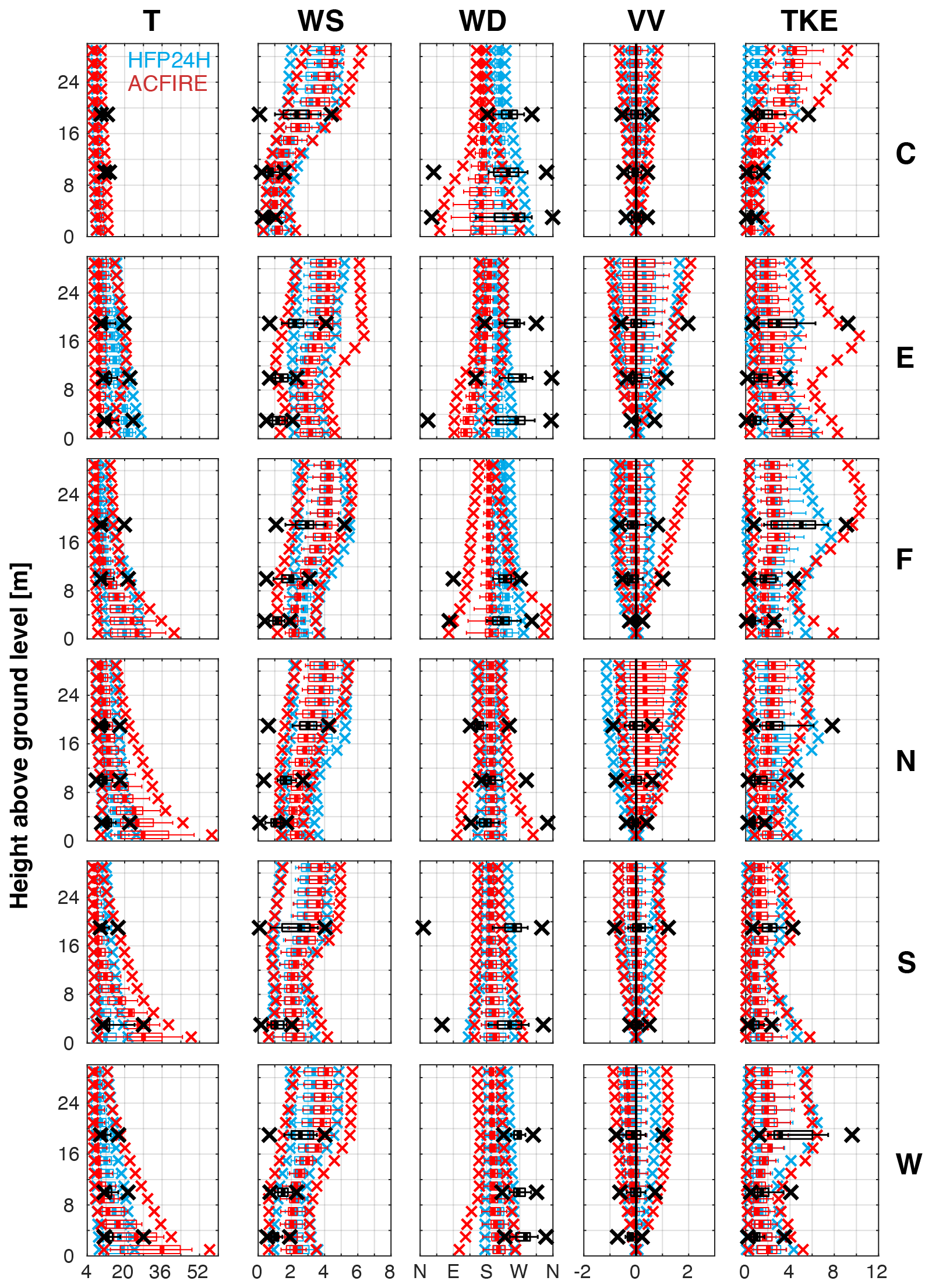
Figure 2Box and whisker plot vertical profiles of 1 min mean temperature (T; °C), wind speed (WS; m s−1), wind direction (WD; °), vertical velocity (VV; m s−1), and turbulent kinetic energy (TKE; m2 s−2) for the Kiefer et al. (2022) simulation yielding the best overall agreement with observations (HFP24H; blue) and the present ACFIRE simulation (ACFIRE; red) at all towers (labeled along the right axis, with locations depicted in Fig. 1). Box and whisker plots are constructed from 40 1 min mean values ± 20 min from the time of peak 1 min mean observed heat flux, except for TWRC , wherein 15:20 EDT is chosen arbitrarily: TWRE is centered at 15:42 EDT, TWRF is centered at 15:28 EDT, TWRN is centered at 16:20 EDT, TWRS is centered at 15:08 EDT, and TWRW is centered at 15:38 EDT. For each box and whisker plot, the thick line denotes the median, the boxes extend outward to the 25th and 75th percentiles, the whiskers extend outward to the 10th and 90th percentiles, and the “x” symbols indicate the minimum and maximum values. Tower observations (O) and model-simulated values (M) are indicated by black and red colors, respectively (see the legend in the top-left panel). The vertical black line in the VV column corresponds to zero vertical velocity. The x axis in the WD column is labeled as follows: N (0/360°), E (90°), S (180°), W (270°). Manual quality control of tower observations results in the exclusion of three data points: lower tower level T at TWRC and TWRF and upper tower level WD at TWRF.
To assess the performance of ACFIRE relative to HFP24H, box and whisker plot vertical profiles of simulated and observed temperature, wind speed, wind direction, vertical velocity, and TKE at each flux tower are presented in Fig. 2. Close examination of Fig. 2 along with supporting statistics (not shown) reveals that overall ACFIRE performs as well or better than HFP24H in representing atmospheric variables at the six flux towers. Specifically, the greatest improvement of ACFIRE over HFP24H is seen in the simulation of upper-canopy TKE. At TWRW, the tower at which the Kiefer et al. (2022) model sensitivity assessment was performed, TKE root-mean square difference (RMSD) as a percentage of the observed range of values decreases from 42.4 % for HFP24H to 36.6 % for ACFIRE. Furthermore, the model-simulated 40 min maximum upper-canopy TKE is approximately equal to the corresponding observations at TRWE, TWRF, and TWRS. However, this improvement in the simulated upper-canopy TKE comes at a cost of the agreement between the simulated and observed lower-canopy variables at some towers, most notably for 40 min maximum temperature. This overestimation of lower-canopy variables is likely due to the introduction of DEVS-FIRE sensible heat flux into the lowest ARPS-CANOPY grid layer; distribution of the sensible heat flux vertically within the forest canopy, as in Kiefer et al. (2022), is an important task left for future work. The reader should keep in mind this lower-canopy overestimation of atmospheric variables at some towers when considering the ability of ACFIRE to simulate fire spread rates across the burn block. However, the overall improvement in model-simulated TKE increases confidence in the ability of ACFIRE to capture the fire-perturbed turbulent flow through the forest canopy and in particular the upper-canopy turbulent flow. Although the focus of the present study is on fire spread, the improved representation of turbulent flow in ACFIRE may also have important implications for studies using ARPS-CANOPY wind output to drive smoke dispersion models (as in Charney et al. 2019).
Examination of the ACFIRE simulation continues with a comparison of fire arrival isochrones between the ACFIRE simulation and the fire-tracker observations (Fig. 3). Simulated fire arrival time is defined here as the time when sensible heat flux first exceeds 500 W m−2 at each grid cell (threshold assumed to be representative of background, i.e., non-fire, surface sensible heat fluxes) and observed fire arrival time is defined as the time of maximum positive temperature change at each fire-tracker thermocouple (depicted with black circles in Fig. 3). Observed fire arrival time isochrones are constructed by interpolating individual fire-tracker arrival times to a uniformly spaced 1-m grid using a cubic spatial interpolation. In comparing simulated and observed fire spread patterns, the reader is encouraged to keep in mind the uniform fuel model setting in DEVS-FIRE (Sect. 4.1), the variable spacing between fire-trackers (Fig. 3), the different fire arrival time definitions, and the lack of fire-trackers in the northern 20 % of the burn unit, preventing observed fire arrival isochrones from being drawn there (Fig. 3).

Figure 3Isochrones of fire arrival time (EDT), with 10 min interval (ACFIRE simulation: solid; fire-tracker observation: dashed). Fire-trackers are depicted with small black circles (68 total); note that a plotting error in Kiefer et al. (2022) (their Fig. 1) resulted in 11 undeployed fire-trackers in the northern 20 % of the burn unit being inadvertently plotted therein. Inset panels depict zoomed-in views of two unburned “islands” observed by fire-tracker array.
To begin, the observed southwest to northeast fire spread pattern depicted by the fire-tracker array is reproduced in the model simulation, with the observed and simulated fire front reaching the northeastern perimeter of the burn unit between 16:27 and 16:37 EDT, or about 90 min after ignition along the southwestern perimeter. Given the prevailing southerly wind during the fire (see Fig. 5 in Kiefer et al., 2022), this indicates a predominately heading fire in both the observations and model simulation. Arrival time bias error and root mean square error are 0.9 and 17.6 min, respectively, indicating that the model tends to underestimate fire spread rates, with the fire arriving at the fire-trackers just under one minute too late, on average, in the model. Despite this broad agreement, two prominent features of the observed fire spread pattern are lacking in the ACFIRE simulation: (i) two unburned “islands”, one in the north-central part of the burn unit and the other along the eastern perimeter (Fig. 3, inset panels); and (ii) several “tongues” or “fingers” scattered across the burn unit, with locally enhanced fire spread rates. Compared to the observed fire spread pattern, spread in ACFIRE is relatively homogeneous across the burn unit; close examination of Fig. 3 reveals observed spread rates in the range of about 0.4 to 6.6 m min−1 and simulated spread rates in a much narrower range, from about 2.3 to 3.7 m min−1. Simulated spread rates are generally weakest in the northwestern area of the burn unit and near the eastern perimeter, and strongest in the east-central area of the burn unit where the fire arrival isochrones exhibit a convex or bulging shape. Immediately northwest of the area of convex fire shape is a kink in the simulated fire front, near but not collocated with the north-central unburned island observed by the fire-tracker array. A comparison of canopy spatial heterogeneity in Fig. 1 and the fire arrival time isochrones in Fig. 3 reveals few clues as to the source of the observed and simulated fire spread patterns, although the unburned islands appear to overlap with isolated pockets of less dense and less tall forest vegetation. A more systematic analysis of this relationship is an important direction for future work.
Next, we consider the spatiotemporal evolution of DEVS-FIRE surface sensible heat flux and ARPS-CANOPY 6-m wind speed and direction, as computed on each model grid (3- and 30-m horizontal spacing, respectively), and as spatially interpolated for use by the other model. This analysis serves in part as a check of the ARPS-CANOPY → DEVS-FIRE (bilinear) and DEVS-FIRE → ARPS-CANOPY (numerical average) spatial interpolation procedures inherited from ARPS/DEVS-FIRE (Sect. 2.3); this exercise is motivated by the lack of such an analysis in Dahl et al. (2015). The analysis is presented in two forms, as single images with a 20 min interval between frames (Figs. 3–8); and as an animation with a 1 min interval between frames (Movie S1 in the Supplement, video supplement). Beginning with 15:07 EDT (Fig. 4), corresponding approximately to the end of the 10 min manual ignition period along the southwestern perimeter (Sect. 4.1), the fire at the southern tip of the burn unit (where ignition occurred first) has spread approximately 25 m north-eastward. Instantaneous sensible heat flux values are approximately 160 and 30 kW m−2 on the DEVS-FIRE and ARPS-CANOPY grids, respectively, illustrating the diluting effect of the DEVS-FIRE → ARPS-CANOPY grid interpolation procedure. Note that although latent heat fluxes are also output by DEVS-FIRE and ingested by ARPS-CANOPY, they are about one order of magnitude smaller than the sensible heat fluxes and are not shown here. An assessment of the relative impacts of sensible vs. latent heat fluxes on the fire-perturbed atmospheric flow and two-way fire-atmosphere coupling in ACFIRE is left to future work.

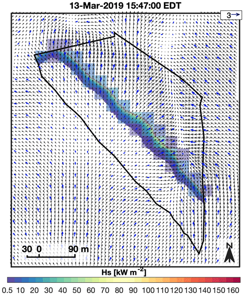
Figure 4Overlay of fire sensible heat flux and 6-m wind speed, direction on ARPS-CANOPY (blue arrows) and DEVS-FIRE (black arrows) grids, at 15:07 EDT. Wind vectors are displayed at every ARPS-CANOPY grid point and every third DEVS-FIRE grid point, the reference vector is depicted in the lower-right corner, and heat flux values less than 0.5 kW m−2 are masked. See Movie S1 (video supplement) for corresponding animation with 1 min interval.
Examining the wind vectors in Fig. 4 next, an apparently turbulent wind field is present in and surrounding the burn unit with instantaneous 6-m AGL wind speed (direction) in the range of about 0–3 m s−1 (0–360°), embedded within a predominately southerly wind field. One-minute mean total (grid-resolved plus SGS) TKE values associated with the resolved and unresolved turbulent eddies are on the order of 2–8 m2 s−2 in the lower canopy (Fig. 2). The horizontal scale of grid-resolved turbulent eddies in Fig. 4 is on the order of 100 m, corresponding to about three times the ARPS-CANOPY horizontal grid spacing in the D5 domain (30 m, Table 1). This is an important detail that must be kept in mind when interpreting the results of this study: the use of 30-m horizontal grid spacing implies that only very large turbulent eddies with spatial scales on the order of 100 m or more are explicitly resolved on the model grid. All other scales of turbulence are parameterized by the model using a 1.5-order TKE closure (Table 2); for context, SGS TKE values in the simulation are about one order of magnitude smaller than the grid-resolved TKE values (not shown). The absence of finer-scale explicitly-resolved turbulent eddies is likely a contributing factor to the overall smooth appearance of the simulated fire arrival isochrones in Fig. 3, in addition to the smoothing influence of the grid interpolation procedure and the impact of horizontally-homogeneous fuels in DEVS-FIRE. Lastly, careful comparison of sensible heat fluxes and winds on the two model grids suggests an absence of aliasing or distortion effects associated with the grid interpolation procedures in ACFIRE.
By 15:27 EDT (Fig. 5), the fire has progressed away from the southwestern perimeter, largely retaining the linear shape it inherited from the perimeter where ignition first occurred. The one deviation from this overall shape is at the northern end of the fire where a rounded “cane” shape has developed. Regrettably, the lack of fire-trackers in the northern 20 % of the burn unit prevents the validation of this curved feature. Interestingly, the wind vectors depict a south-north oriented convergence axis that extends about 100–200 m north of the fire center. Positive vertical velocities associated with this feature increase with height through the forest canopy, exceeding +2 m s−1 at 19 (not shown). Examination of Movie S1 in the Supplement (video supplement) reveals this feature to be somewhat transient in nature and not anchored to any one area of the fire. By 15:47 EDT (Fig. 6), two new fire shape features have developed: (i) a slightly bowed segment near the approximate center of the burn unit, and (ii) a lagging segment near the eastern perimeter. In searching for the source(s) of these two emergent features, the reader is encouraged to consider the 1 min interval animation in Movie S1 (video supplement), especially between about 15:37 and 15:47 EDT: enhanced fire-normal (fire-parallel) winds and larger (smaller) fire spread rates develop near the fire center (eastern end). These features are associated with the aforementioned area of convergent flow that tends to predominate ahead (i.e., north) of the fire. These statements are confirmed by an analysis of animations with a 1 s interval between frames (not shown).

Figure 5Overlay of fire sensible heat flux and 6-m wind speed, direction on ARPS-CANOPY (blue arrows) and DEVS-FIRE (black arrows) grids, at 15:27 EDT. Wind vectors are displayed at every ARPS-CANOPY grid point and every third DEVS-FIRE grid point, the reference vector is depicted in the lower-right corner, and heat flux values less than 0.5 kW m−2 are masked. See Movie S1 (video supplement) for corresponding animation with 1 min interval.

Figure 6Overlay of fire sensible heat flux and 6-m wind speed, direction on ARPS-CANOPY (blue arrows) and DEVS-FIRE (black arrows) grids, at 15:47 EDT. Wind vectors are displayed at every ARPS-CANOPY grid point and every third DEVS-FIRE grid point, the reference vector is depicted in the lower-right corner, and heat flux values less than 0.5 kW m−2 are masked. See Movie S1 (video supplement) for corresponding animation with 1 min interval.
Proceeding to 16:07 EDT (Fig. 7), the emergent features (bowed fire front and lagging segment) have become more pronounced. The bowed fire front is broadly similar to the parabolic head fire shapes identified in previous coupled atmosphere–fire modeling studies (e.g., Clark et al., 1996a; Mandel et al., 2011; Dahl et al., 2015), shapes that have also been observed during real-world fires (e.g., Cheney et al., 1993; Clements et al., 2007; Mueller et al., 2017; Clements et al., 2019). Interestingly, winds over and adjacent to the bowed fire front are light and variable (≪ 1 m s−1), although the weak flow is a transient condition (cf. 16:05 to 16:09 EDT frames in Movie S1, video supplement). Southeast of this feature, locally enhanced fire-parallel southeast winds are associated with smaller fire spread rates relative to the bowing segment. These aspects of the wind field are embedded within the broader turbulent flow consisting of very large eddies within a convective boundary layer (i.e., non-fire turbulence). A close examination of Movie S1 (video supplement) reveals that in general wind velocities are greater over and downwind (i.e., northeast) of the fire relative to winds upstream (i.e., southwest) of the fire. This suggests that the fire sensible heat source is enhancing the already turbulent flow in the simulated convective boundary layer (as shown in Fig. 2). Stepping forward to 16:27 EDT (Fig. 8), the fire shape has further deviated from the initial linear shape inherited from the southwestern burn unit perimeter where the fire was first ignited. The bowing fire feature has expanded in scale to about 100 m in length, a pronounced kink in the fire front has developed immediately northwest of the bowing segment, and the fire to the southeast of the bowing segment is oriented approximately south-north along the eastern perimeter. The bowing segment reaches the northeastern perimeter of the burn unit at approximately 16:32 EDT (Movie S1, video supplement), approximately five minutes later than was observed by the fire-tracker array. Finally, at 16:47 EDT (Fig. 9), the active burning in the model is limited to near the northeastern perimeter of the burn unit. This is consistent with both the fire-tracker array data and reports by on-site personnel (active burning ended at ∼ 16:45 EDT according to Heilman et al., 2021 and Kiefer et al., 2022).

Figure 7Overlay of fire sensible heat flux and 6-m wind speed, direction on ARPS-CANOPY (blue arrows) and DEVS-FIRE (black arrows) grids, at 16:07 EDT. Wind vectors are displayed at every ARPS-CANOPY grid point and every third DEVS-FIRE grid point, the reference vector is depicted in the lower-right corner, and heat flux values less than 0.5 kW m−2 are masked. See Movie S1 (video supplement) for corresponding animation with 1 min interval.
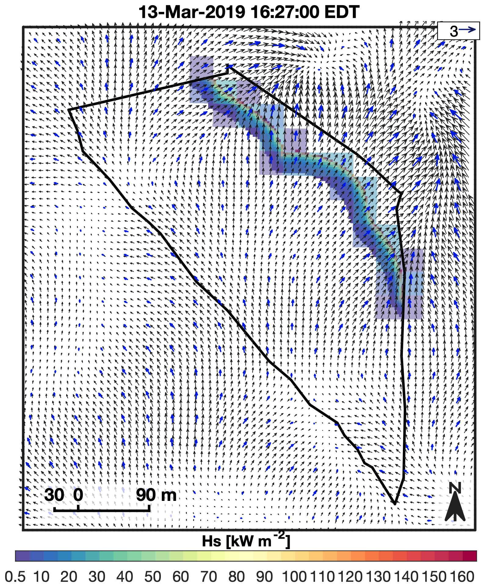
Figure 8Overlay of fire sensible heat flux and 6-m wind speed, direction on ARPS-CANOPY (blue arrows) and DEVS-FIRE (black arrows) grids, at 16:27 EDT. Wind vectors are displayed at every ARPS-CANOPY grid point and every third DEVS-FIRE grid point, the reference vector is depicted in the lower-right corner, and heat flux values less than 0.5 kW m−2 are masked. See Movie S1 (video supplement) for corresponding animation with 1 min interval.
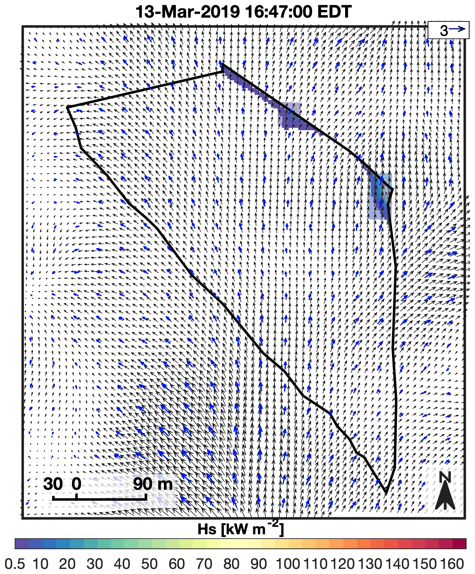
Figure 9Overlay of fire sensible heat flux and 6-m wind speed, direction on ARPS-CANOPY (blue arrows) and DEVS-FIRE (black arrows) grids, at 16:47 EDT. Wind vectors are displayed at every ARPS-CANOPY grid point and every third DEVS-FIRE grid point, the reference vector is depicted in the lower-right corner, and heat flux values less than 0.5 kW m−2 are masked. See Movie S1 (video supplement) for corresponding animation with 1 min interval.
This study introduced ACFIRE version 1.0, a mesoscale model containing a forest canopy sub-model (ARPS-CANOPY) and a fire behavior sub-model (DEVS-FIRE), and detailed its development and preliminary evaluation. ACFIRE is intended to fill a gap in the existing collection of coupled atmosphere–fire models (Sect. 1.1) by combining (i) the ability to simulate the effects of a wildland fire on the atmosphere hundreds of meters to hundreds of kilometers away, (ii) a broad suite of physical parameterizations, and (iii) the capability of explicitly resolving some scales of atmospheric turbulence within and above a forest canopy. In this study, ACFIRE was used to simulate the evolution of a low-intensity prescribed fire conducted in the New Jersey Pine Barrens in March 2019, as part of a broader study of multi-scale fire combustion processes in open-canopied forests. Simulated fire spread patterns and rates were compared to measurements from an array of surface thermocouples deployed during the experiment (fire-tracker array). Comparisons included vertical profiles of atmospheric variables, spatial maps of observed and simulated fire-arrival isochrones, and overlayed plots of surface sensible heat fluxes and 6-m AGL winds within and surrounding the burn unit.
The ACFIRE simulation generally captured the mean and turbulent flow through the forest canopy and considerably improved upon ARPS-CANOPY with an imposed heat source in representing upper-canopy TKE. The ACFIRE simulation also successfully captured the overall fire spread, both in terms of spread rates, which were within the range of fire-tracker observed spread rates, and in terms of the transit time for the fire to spread across the burn unit. Where the model simulation fell short was in the finer-scale details of fire spread; for example, the simulation did not reproduce unburned patches and exhibited a narrower spread rate range compared to observations. Considering the use of homogeneous fuels in DEVS-FIRE and relatively coarse 30-m × 30-m grid cells in ARPS-CANOPY, the overall agreement between the ACFIRE simulation and the fire-tracker observations is encouraging. Furthermore, the fact that the ACFIRE simulation was run without any form of model nudging or data assimilation for 2 h post-ignition without any gross deviations from the observed fire spread pattern is particularly encouraging. It is important to note, however, that ACFIRE has been evaluated here using a single prescribed fire case in a small (∼ 11 ha) burn unit consisting of generally horizontally homogeneous fuels. Application of ACFIRE to other cases, including both prescribed fires and wildfires, remains an important task for future work.
Specific next steps include ACFIRE simulations with (i) DEVS-FIRE sensible heat flux distributed vertically within the forest canopy, (ii) heterogeneous fuels; (iii) higher-intensity fires (e.g., those associated with grassy fuels); (iv) horizontal grid spacing on the order of 1 m, allowing a larger proportion of in-canopy turbulence to be resolved on the model grid; (v) longer-duration fires, including multi-day events; (vi) fires with burn areas of 100 ha or greater; and (vii) fires in complex terrain. These and other ACFIRE simulations are expected to yield useful insights into the performance of ACFIRE under different fire-fuels-atmosphere configurations.
As stated previously, ACFIRE is exclusively a surface fire spread model. Future plans include the implementation of the Scott and Reinhardt (2001) crown fire modeling approach in ACFIRE, maintaining the Rothermel (1972) model of surface fire spread and introducing the Rothermel (1991) crown fire equations and Van Wagner (1977) method of surface-crown fire transition. A key aspect of this future work will be the modification of Ap profile data to reflect the consumption of canopy fuels by the crown fire.
Finally, the replacement of the user-imposed fire heat source in ARPS-CANOPY with a heat source computed dynamically in DEVS-FIRE is an important step in the development of the ARPS-CANOPY model. In time, ACFIRE is expected to contribute to community knowledge of fire-atmosphere interactions in much the same way that ARPS-CANOPY with a user-imposed fire heat source has up to this point. Models like ACFIRE offer a controlled framework for exploring and quantifying the key mechanisms that drive fire–fuel–atmosphere interactions. Insights gained from such modeling systems can support the development of new or improved parameterizations suitable for inclusion in simpler operational models, potentially enhancing their ability to represent dynamic fire behavior under more realistic, transient conditions.
Data sets and software code associated with this study have been uploaded to the Harvard Dataverse (https://doi.org/10.7910/DVN/WECMQW, Kiefer et al., 2025). Data are available under the terms of the Creative Commons Zero “No rights reserved” data waiver (CC0 1.0 Public domain dedication). The DEVS-FIRE model is not open source because it is based on DEVSJAVA that is copyrighted by the University of Arizona. Furthermore, we are considering the option of commercializing the DEVS-FIRE software to better serve the community. Due to these reasons, we cannot make the DEVS-FIRE source code publicly available. Instead, we would be happy to provide confidential access to the DEVS-FIRE code for the editor and reviewers.
Overlay of fire sensible heat flux and 6-m wind speed, direction on ARPS-CANOPY (blue arrows) and DEVS-FIRE (black arrows) grids, at 1 min interval, from 14:57 to 16:57 EDT 13 March 2019; compare to 15:07 to 16:47 EDT static images in Figs. 4–9. Wind vectors are displayed at every ARPS-CANOPY grid point and every third DEVS-FIRE grid point, the reference vector is depicted in the upper-right corner, and heat flux values less than 0.5 kW m−2 are masked. It is available at: https://doi.org/10.5281/zenodo.23768351 (Kiefer et al., 2026).
MTK, WEH, SZ, and JJC contributed to the conceptualization of the study. MTK developed the methodology and conducted the numerical analyses, with WEH, SZ, JJC, XB, and JS assisting in the interrogation and refinement of the analyses. MTK wrote and prepared the original manuscript draft, with editorial contributions from SZ and additional feedback from SZ and WEH. MTK and SZ revised the manuscript in response to the review comments. All co-authors reviewed the manuscript before submission. NSS, KLC, MRG, JC and MP were responsible for the collection and preparation of the field data used to validate the model results, and EVM processed the fire-tracker array data. MTK and XH served as the ARPS-CANOPY and DEVS-FIRE technical experts, respectively, and MTK curated the model study data archive.
The contact author has declared that none of the authors has any competing interests.
Publisher's note: Copernicus Publications remains neutral with regard to jurisdictional claims made in the text, published maps, institutional affiliations, or any other geographical representation in this paper. The authors bear the ultimate responsibility for providing appropriate place names. Views expressed in the text are those of the authors and do not necessarily reflect the views of the publisher.
Special thanks are given to the New Jersey Forest Fire Service for conducting the burn. The color schemes used in all figures were developed by Cynthia Brewer at the Pennsylvania State University (http://colorbrewer2.org/, last access: 27 June 2025).
This research has been supported by the U.S. Forest Service (grant no. RJVA 21-CS-11242306-055) and the National Institute of Food and Agriculture (grant no. Hatch Project MICL02754).
This paper was edited by Chiel van Heerwaarden and reviewed by two anonymous referees.
Ahmadov, R., Grell, G., James, E., Freitas, S., Pereira, G., Csiszar, I., Tsidulko, M., Pierce, B., McKeen, S., Peckham, S., Alexander, C., Saide, P., and Benjamin, S.: A High Resolution Coupled Meteorology-Smoke Modeling System HRRR-Smoke to Simulate Air Quality over the CONUS Domain in Real Time, Geophys. Res. Abstr., 19, EGU2017–10841, https://meetingorganizer.copernicus.org/EGU2017/EGU2017-10841.pdf (last access: 3 April 2025), 2017.
Ahmadov, R., James, E., Grell, G., Alexander, C., and McKeen, S.: Operational Implementation of the Smoke Forecasting Capability in the RAP/HRRR Numerical Weather Prediction System, in: EGU General Assembly 2021, online, 19–30 April 2021, EGU21-14268, https://doi.org/10.5194/egusphere-egu21-14268, 2021.
Albini, F. A. and Baughman, R. G.: Estimating windspeeds for predicting wildland fire behavior, Res. Pap. INT-221, U.S. Department of Agriculture, Forest Service, Intermountain Forest and Range Experiment Station, https://www.frames.gov/documents/behaveplus/publications/Albini_and_Baughman_1979_INT-RP-221_ocr.pdf (last access: 30 June 2025), 1979.
Anderson, H. E.: Aids to Determining Fuel Models for Estimating Fire Behavior, Gen. Tech. Rep. INT-122, U.S. Department of Agriculture, Forest Service, Intermountain Forest and Range Experiment Station, https://www.fs.usda.gov/rm/pubs_int/int_gtr122.pdf (last access: 3 April 2025), 1982.
Andrews, P. L.: BEHAVE: fire behavior prediction and fuel modeling system – BURN Subsystem, Part 1, General Technical Report INT-194, U.S. Department of Agriculture, Forest Service, Intermountain Research Station, Ogden, UT, 130 p https://doi.org/10.2737/INT-GTR-194 (last access: 24, November 2025), 1986.
Andrews, P. L.: Modeling Wind Adjustment Factor and Midflame Wind Speed for Rothermel's Surface Fire Spread Model, U.S. Department of Agriculture, Forest Service, Intermountain Forest and Range Experiment Station, https://www.fs.usda.gov/rm/pubs/rmrs_gtr266.pdf (last access: 3 April 2025), 2012.
Andrews, P. L. and Chase, C. H.: BEHAVE: fire behavior prediction and fuel modeling system – BURN subsystem, Part 2, General Technical Report INT-GTR-260, U.S. Department of Agriculture, Forest Service, Intermountain Research Station, Ogden, UT, 93 p. https://doi.org/10.2737/INT-GTR-260 (last access: 24, November 2025), 1989.
Banerjee, T.: The Role of Canopy Turbulence in Wildland Fire Behavior, Annu. Rev. Fluid Mech., 58, 473–502, https://doi.org/10.1146/annurev-fluid-112723-062216, 2026.
Baughman, R. G. and Albini, F. A.: Estimating Midflame Windspeeds, in: Proceedings of Sixth Conference on Fire and Forest Meteorology, 22–24 April 1980, Seattle, WA, USA, https://www.frames.gov/documents/behaveplus/publications/Baughman_and_Albini_1980_EstMidflamWind_ocr.pdf (last access: 3 April 2025), 1980.
Burgan, R. E. and Rothermel, R. C.: BEHAVE: fire behavior prediction and fuel modeling system–FUEL subsystem, General Technical Report INT-167, U.S. Department of Agriculture, Forest Service, Intermountain Forest and Range Experiment Station, Ogden, UT, 126 p. https://doi.org/10.2737/INT-GTR-167 (last access: 24, November 2025), 1984.
Charney, J. J., Kiefer, M. T., Zhong, S., Heilman, W. E., Nikolic, J., Bian, X., Hom, J. L., Clark, K. L., Skowronski, N. S., Gallagher, M. R., Patterson, M., Liu, Y., and Hawley, C.: Assessing Forest Canopy Impacts on Smoke Concentrations Using a Coupled Numerical Model, Atmosphere, 10, 273, https://doi.org/10.3390/atmos10050273, 2019.
Cheney, N. P., Gould, J. S., and Catchpole, W. R.: The Influence of Fuel, Weather and Fire Shape Variables on Fire-Spread in Grasslands, Int. J. Wildland Fire, 3, 31–44, https://doi.org/10.1071/WF9930031, 1993.
Chou, M.-D.: Parameterization for the Absorption of Solar Radiation by O2 and CO2 with Application to Climate Studies, J. Climate, 3, 209–217, https://doi.org/10.1175/1520-0442(1990)003<0209:PFTAOS>2.0.CO;2, 1990.
Chou, M.-D.: A Solar Radiation Model for Use in Climate Studies, J. Atmos. Sci., 49, 762–772, https://doi.org/10.1175/1520-0469(1992)049<0762:ASRMFU>2.0.CO;2, 1992.
Chou, M.-D. and Suarez, M. J.: An Efficient Thermal Infrared Radiation Parameterization for use in General Circulation Models, Tech. Rep. Tech. Memo 104606, NASA, NASA Center for Aerospace Information, 800 Elkridge Landing Road, Linthicum Heights, MD 21090-2934, https://ntrs.nasa.gov/api/citations/19950009331/downloads/19950009331.pdf (last access: 13 November 2026), 1994.
Chow, F. K., Schär, C., Ban, N., Lundquist, K. A., Schlemmer, L., and Shi, X.: Crossing Multiple Gray Zones in the Transition from Mesoscale to Microscale Simulation over Complex Terrain, Atmosphere, 10, 274, https://doi.org/10.3390/atmos10050274, 2019.
Chow, F. K., Yu, K. A., Young, A., James, E., Grell, G. A., Csiszar, I., Tsidulko, M., Freitas, S., Pereira, G., Giglio, L., Friberg, M. D., and Ahmadov, R.: High-Resolution Smoke Forecasting for the 2018 Camp Fire in California, B. Am. Meteorol. Soc., 103, E1531–E1552,https://doi.org/10.1175/BAMS-D-20-0329.1, 2022.
Clark, K. L., Heilman, W. E., Skowronski, N. S., Gallagher, M. R., Mueller, E., Hadden, R. M., and Simeoni, A.: Fire Behavior, Fuel Consumption, and Turbulence and Energy Exchange during Prescribed Fires in Pitch Pine Forests, Atmosphere, 11, 242, https://doi.org/10.3390/atmos11030242, 2020.
Clark, T. L., Jenkins, M. A., Coen, J., and Packham, D.: A Coupled Atmospheric-Fire Model: Convective Feedback on Fire Line Dynamics, J. Appl. Meteorol., 35, 875–901, https://doi.org/10.1175/1520-0450(1996)035%3C0875:ACAMCF%3E2.0.CO;2, 1996a.
Clark, T. L., Jenkins, M. A., Coen, J., and Packham, D. A.: A Coupled Atmosphere-Fire Model: Role of the Convective Froude Number and Dynamic Fingering at the Fireline, Int. J. Wildland Fire, 6, 177–190, https://doi.org/10.1071/WF9960177, 1996b.
Clark, T. L., Radke, L., Coen, J., and Middleton, D.: Analysis of Scale-Scale Convective Dynamics in a Crown Fire Using Infrared Video Camera Imagery, J. Appl. Meteorol., 38, 1401–1420, https://doi.org/10.1175/1520-0450(1999)038%3C1401:AOSSCD%3E2.0.CO;2, 1999.
Clark, T. L., Coen, J. L., and Latham, D.: Description of a Coupled Atmosphere-Fire Model, Int. J. Wildland Fire, 13, 49–63, https://doi.org/10.1071/WF03043, 2004.
Clements, C. B., Zhong, S., Goodrick, S., Li, J., Potter, B. E., Bian, X., Heilman, W. E., Charney, J. J., Perna, R., Jang, M., and Lee, D.: Observing the Dynamics of Wildland Grass Fires: FireFlux – A Field Validation Experiment, B. Am. Meteorol. Soc., 88, 1369–1382, 2007.
Clements, C. B., Kochanski, A. K., Seto, D., Davis, B., Camacho, C., Lareau, N. P., Contezac, J., Restaino, J., Heilman, W. E., Krueger, S. K., Butler, B., Ottmar, R. D., Vihnanek, R., Flynn, J., Filippi, J.-B., Barboni, T., Hall, D. E., Mandel, J., Jenkins, M. A., O'Brien, J., Hornsby, B., and Teske, C.: The FireFlux II Experiment: A Model-Guided Field Experiment to Improve Understanding of Fire–Atmosphere Interactions and Fire Spread, Int. J. Wildland Fire, 28, 308–326, https://doi.org/10.1071/WF18089, 2019.
Coen, J. L.: Simulation of the Big Elk Fire Using Coupled Atmosphere-Fire Modeling, Int. J. Wildland Fire, 14, 49–59, https://doi.org/10.1071/WF04047, 2005.
Coen, J. L.: Modeling Wildland Fires: A Description of the Coupled Atmosphere-Wildland Fire Environment Model (CAWFE), National Corporation for Atmospheric Research (NCAR) Technical Note NCAR/TN-500+STR, NCAR, https://opensky.ucar.edu/system/files/2024-08/technotes_511.pdf (last access: 3 April 2025), 2013.
Coen, J. L.: Some Requirements for Simulating Wildland Fire Behavior Using Insight from Coupled Weather – Wildland Fire Models, Fire, 1, 6, https://doi.org/10.3390/fire1010006, 2018.
Dahl, N., Xue, H., Hu, X. and Xue, M.: Coupled Fire–Atmosphere Modeling of Wildland Fire Spread Using DEVS-FIRE and ARPS, Nat. Hazards, 77, 1013–1035, https://doi.org/10.1007/s11069-015-1640-y, 2015.
Deardorff, J. W.: Stratocumulus-Capped Mixed Layers Derived from a Three-Dimensional Model, Bound.-Lay. Meteorol., 18, 495–527, https://doi.org/10.1007/BF00119502, 1980.
Dudhia, J.: A History of Mesoscale Model Development, Asia-Pac. J. Atmos. Sci., 50, 121–131, https://doi.org/10.1007/s13143-014-0031-8, 2014.
Dupont, S. and Brunet, Y.: Influence of Foliar Density Profile on Canopy Flow: A Large-Eddy Simulation Study, Agr. Forest. Meteorol., 148, 976–990, https://doi.org/10.1016/j.agrformet.2008.01.014, 2008.
Filippi, J.-B., Bosseur, F., Pialat, X., Santoni, P.-A., Strada, S., and Mari, C.: Simulation of Coupled Fire/Atmosphere Interaction with the MesoNH-ForeFire Models, J. Combust., 2011, 540390, https://doi.org/10.1155/2011/540390, 2011.
Filippi, J.-B., Pialat, X., and Clements, C. B.: Assessment of ForeFire/Meso-NH for Wildland Fire/Atmosphere Coupled Simulation of the FireFlux Experiment, Proc. Combust. Inst., 34, 2633–2640, https://doi.org/10.1016/j.proci.2012.07.022, 2013.
Finney, M. A.: FARSITE: Fire Area Simulator-model development and evaluation, Res. Pap. RMRS-RP-4, Revised 2004, U.S. Department of Agriculture, Forest Service, Rocky Mountain Research Station, Ogden, UT, 47 p, https://doi.org/10.2737/RMRS-RP-4 (last access: 24, November 2025), 1998.
Finney, M. A.: An Overview of FlamMap Fire Modeling Capabilities, in: comps. 2006. Fuels Management-How to Measure Success: Conference Proceedings. 28–30 March 2006, Portland, OR, edited by: Andrews, P. L. and Butler, B. W., Proceedings RMRS-P-41, U.S. Department of Agriculture, Forest Service, Rocky Mountain Research Station, Fort Collins, CO, p. 213–220, https://research.fs.usda.gov/treesearch/25948 (last access: 24 Novermber 2025), 2006.
Finnigan, J. J.: Turbulence in Plant Canopies, Annu. Rev. Fluid Mech., 32, 519–571, https://doi.org/10.1146/annurev.fluid.32.1.519, 2000.
Gallagher, M. R., Skowronski, N. S., Hadden, R. M., Mueller, E. V., Clark, K. L., Campbell-Lochrie, Z. J., Walker-Ravena, C., Kremens, R. L., Everland, A. I., Patterson, M. M., Cole, J. A., Heilman, W. E., Charney, J. J., Bian, X., Mell, W. E., Hom, J. L., Im, S.-K., Kiefer, M. T., Zhong, S., Simeoni, A. J., Rangwala, A., Di Cristina, G., and Sietz, J.: Multi-scale analyses of wildland fire combustion processes: Large-scale field experiments – burn layout and documentation, USDA Forest Service Research Data Archive [data set], https://doi.org/10.2737/RDS-2022-0089, 2023.
Heilman, W. E., Clements, C. B., Seto, D., Bian, X., Clark, K. L., Skowronski, N. S., and Hom, J. L.: Observations of Fire-Induced Turbulence Regimes During Low-Intensity Wildland Fires in Forested Environments: Implications for Smoke Dispersion, Atmos. Sci. Lett., 16, 453–460, https://doi.org/10.1002/asl.581, 2015.
Heilman, W. E., Clark, K. L., Bian, X., Charney, J. J., Zhong, S., Skowronski, N. S., Gallagher, M. R., and Patterson, M.: Turbulent Momentum Flux Behavior above a Fire Front in an Open-Canopied Forest, Atmosphere, 12, 956, https://doi.org/10.3390/atmos12080956, 2021.
Heilman, W. E.: Atmospheric turbulence and wildland fires: a review, Int. J. Wildland Fire, 32, 476–495, https://doi.org/10.1071/WF22053, 2023.
Hiers, J. K., Ottmar, R., Butler, B. W., Clements, C., Vihnanek, R., Dickinson, M. B., and O'Brien, J.: An Overview of the Prescribed Fire Combustion and Atmospheric Dynamics Research Experiment (Rx-CADRE), in: 4th International Fire Ecology and Management Congress: Fire as a Global Process, 30 November–5 December 2009, Savannah, Georgia, USA, edited by: Rideout-Hanzak, S., https://doi.org/10.4996/fireecology.0701001, 2009.
Hoffman, C. M., Linn, R., Parsons, R., Sieg, C., and Winterkamp, J.: Modeling Spatial and Temporal Dynamics of Wind Flow and Potential Fire Behavior Following a Mountain Pine Beetle Outbreak in a Lodgepole Pine Forest, Agr. Forest. Meteorol., 204, 79–93, https://doi.org/10.1016/j.agrformet.2015.01.018, 2015.
Huang, H.: Modeling the inhibition effect of straw checkerboard barriers on wind-blown sand, Earth Surf. Dynam., 11, 167–181, https://doi.org/10.5194/esurf-11-167-2023, 2023.
Kiefer, M. T. and Zhong, S.: An Idealized Modeling Study of Nocturnal Cooling Processes Inside a Small Enclosed Basin, J. Geophys. Res., 116, D20127, https://doi.org/10.1029/2011JD016119, 2011.
Kiefer, M. T. and Zhong, S.: The Effect of Sidewall Forest Canopies on the Formation of Cold-Air Pools – A Numerical Study, J. Geophys. Res., 118, 5965–5978, https://doi.org/10.1002/jgrd.50509, 2013.
Kiefer, M. T. and Zhong, S.: The Role of Forest Cover and Valley Geometry in Cold-Air Pool Evolution, J. Geophys. Res., 120, 8693–8711, https://doi.org/10.1002/2014JD022998, 2015.
Kiefer, M. T., Lin, Y.-L., and Charney, J. J.: A Study of Two-Dimensional Dry Convective Plume Modes with Variable Critical Level Height, J. Atmos. Sci., 65, 448–469, https://doi.org/10.1175/2007JAS2301.1, 2008.
Kiefer, M. T., Parker, M. D., and Charney, J. J.: Regimes of Dry Convection Above Wildfires: Idealized Numerical Simulations and Dimensional Analysis, J. Atmos. Sci., 66, 806–836, https://doi.org/10.1175/2008JAS2896.1, 2009.
Kiefer, M. T., Parker, M. D., and Charney, J. J.: Regimes of Dry Convection Above Wildfires: Sensitivity to Fireline Details, J. Atmos. Sci., 67, 611–632, https://doi.org/10.1175/2009JAS3226.1, 2010.
Kiefer, M. T., Zhong, S., Heilman, W. E., Charney, J. J., and Bian, X.: Evaluation of an ARPS-Based Canopy Flow Modeling System for use in Future Operational Smoke Prediction Efforts, J. Geophys. Res., 118, 6175–6188, https://doi.org/10.1002/jgrd.50491, 2013.
Kiefer, M. T., Heilman, W. E., Zhong, S., Charney, J. J., Bian, X., Skowronski, N. S., Hom, J. L., Clark, K. L., Patterson, M., and Gallagher, M. R.: Multiscale Simulation of a Prescribed Fire Event in the New Jersey Pine Barrens using ARPS-CANOPY, J. Appl. Meteorol. Clim., 53, 793–812, https://doi.org/10.1175/JAMC-D-13-0131.1, 2014.
Kiefer, M. T., Heilman, W. E., Zhong, S., Charney, J. J., and Bian, X.: Mean and Turbulent Flow Downstream of a Low-Intensity Fire: Influence of Canopy and Background Atmospheric Conditions, J. Appl. Meteorol. Clim., 54, 42–57, https://doi.org/10.1175/JAMC-D-14-0058.1, 2015.
Kiefer, M. T., Heilman, W. E., Zhong, S., Charney, J. J., and Bian, X.: A study of the influence of forest gaps on fire–atmosphere interactions, Atmos. Chem. Phys., 16, 8499–8509, https://doi.org/10.5194/acp-16-8499-2016, 2016.
Kiefer, M. T., Zhong, S., Heilman, W. E., Charney, J. J., and Bian, X.: A Numerical Study of Atmospheric Perturbations Induced by Heat from a Wildland Fire: Sensitivity to Vertical Canopy Structure and Heat Source Strength, J. Geophys. Res., 123, 2555–2572, https://doi.org/10.1002/2017JD027904, 2018.
Kiefer, M. T., Charney, J. J., Zhong, S., Heilman, W. E., Bian, X., Hom, J. L., and Patterson, M.: Evaluation of the Ventilation Index in Complex Terrain: A Dispersion Modeling Study. J. Appl. Meteorol. Clim., 58, 551–568, https://doi.org/10.1175/JAMC-D-18-0201.1, 2019.
Kiefer, M. T., Charney, J. J., Zhong, S., Heilman, W. E., Bian, X., and Mathewson, T. O.: A Numerical Modeling Study of Smoke Dispersion and the Ventilation Index in Southwestern Colorado, Atmosphere, 11, 846, https://doi.org/10.3390/atmos11080846, 2020.
Kiefer, M. T., Heilman, W. E., Zhong, S., Charney, J. J., Bian, X., Skowronski, N. S., Clark, K. L., Gallagher, M. R., Hom, J. L., and Patterson, M.: Representing low-intensity fire sensible heat output in a mesoscale atmospheric model with a canopy submodel: a case study with ARPS-CANOPY (version 5.2.12), Geosci. Model Dev., 15, 1713–1734, https://doi.org/10.5194/gmd-15-1713-2022, 2022.
Kiefer, M. T., Zhong, S., Charney, J. J., Bian, X., Heilman, W. E., Seitz, J., Skowronski, N. S., Clark, K. L., Gallagher, M. R., Hom, J. L., Patterson, M., Mueller, E. V., and Hu, X: Development of ACFIRE version 1.0: A mesoscale model with forest canopy and fire behaviour submodels, Harvard Dataverse [data set], https://doi.org/10.7910/DVN/WECMQW, 2025.
Kiefer, M. T., Zhong, S., Charney, J. J., Bian, X., Heilman, W.E., Seitz, J., Skowronski, N. S., Clark, K. L., Gallagher, M. R., Hom, J. L., Patterson, M., Mueller, E. V., and Hu, X: Animation of DEVS-FIRE sensible heat flux and ARPS-CANOPY wind speed and direction, Zenodo [video], https://doi.org/10.5281/zenodo.23768351, 2026.
Kochanski, A. K., Jenkins, M. A., Yedinak, K., Mandel, J., Beezley, J., and Lamb, B.: Toward an Integrated System for Fire, Smoke and Air Quality Simulations, Int. J. Wildland Fire, 25, 534–546, https://doi.org/10.1071/WF14074, 2016.
Kochanski, A. K., Fournier, A., and Mandel, J.: Experimental Design of a Prescribed Burn Instrumentation, Atmosphere, 9, 296, https://doi.org/10.3390/atmos9080296, 2018.
Linn, R., Reisner, J., Colman, J. J., and Winterkamp, J.: Studying Wildfire Behavior Using FIRETEC, Int. J. Wildland Fire, 11, 233–246, https://doi.org/10.1071/WF02007, 2002.
Linn, R. R., Goodrick, S. L., Brambilla, S., Brown, M. J., Middleton, R. S., O'Brien, J., and Hiers, J. K.: QUIC-fire: A Fast-Running Simulation Tool for Prescribed Fire Planning, Environ. Model. Softw., 125, 104616, https://doi.org/10.1016/j.envsoft.2019.104616, 2020.
Linn, R. R., Winterkamp, J. L., Furman, J. H., Williams, B., Hiers, J. K., Jonko, A., O'Brien, J. J., Yedinak, K. M., and Goodrick, S.: Modeling Low Intensity Fires: Lessons Learned from 2012 RxCADRE, Atmosphere, 12, 139, https://doi.org/10.3390/atmos12020139, 2021.
Luderer, G., Trentmann, J., Winterrath, T., Textor, C., Herzog, M., Graf, H. F., and Andreae, M. O.: Modeling of biomass smoke injection into the lower stratosphere by a large forest fire (Part II): sensitivity studies, Atmos. Chem. Phys., 6, 5261–5277, https://doi.org/10.5194/acp-6-5261-2006, 2006.
Ma, Y. and Liu, H.: An Advanced Multiple-Layer Canopy Model in the WRF model with Large-Eddy Simulations to Simulate Canopy Flows and Scalar Transport Under Different Stability Conditions, J. Adv. Model. Earth Sy., 11, 2330–2351, https://doi.org/10.1029/2018MS001347, 2019.
Mallia, D. V., Kochanski, A. K., Urbanski, S. P., and Lin, J. C.: Optimizing Smoke and Plume Rise Modeling Approaches at Local Scales, Atmosphere, 9, 166, https://doi.org/10.3390/atmos9050166, 2018.
Mallia, D. V., Kochanski, A. K., Urbanski, S. P., Mandel, J., Farguell, A., and Krueger, S. K.: Incorporating a Canopy Parameterization within a Coupled Fire-Atmosphere Model to Improve a Smoke Simulation for a Prescribed Burn, Atmosphere, 11, 832, https://doi.org/10.3390/atmos11080832, 2020.
Mandel, J., Beezley, J. D., and Kochanski, A. K.: Coupled atmosphere-wildland fire modeling with WRF 3.3 and SFIRE 2011, Geosci. Model Dev., 4, 591–610, https://doi.org/10.5194/gmd-4-591-2011, 2011.
Mason, P. J.: Large-Eddy Simulation: A Critical Review of the Technique, Q. J. Roy. Meteor. Soc., 120, 1–26, https://doi.org/10.1002/qj.49712051503, 1994.
Massman, W. J., Forthofer, J. M., and Finney, M. A.: An Improved Canopy Wind Model for Predicting Wind Adjustment Factors and Wildland Fire Behavior, Can. J. For. Res., 47, 594–603, https://doi.org/10.1139/cjfr-2016-0354, 2017.
Mell, W., Jenkins, M. A., Gould, J., and Cheney, P.: A Physics-Based Approach to Modelling Grassland Fires, Int. J. Wildland Fire, 16, 1–22, https://doi.org/10.1071/WF06002, 2007.
Moeng, C. H. and Wyngaard, J. C.: Evaluation of Turbulent Transport and Dissipation Closures in Second-Order Modeling, J. Atmos. Sci., 46, 2311–2330, https://doi.org/10.1175/1520-0469(1989)046%3C2311:EOTTAD%3E2.0.CO;2, 1989.
Morvan, D., Accary, G., Meradji, S., and Frangieh, N.: Fifty Years of Progress in Wildland Fire Modelling: From Empirical to Fully Physical CFD Models, C. R. Mecanique, 350, 107–115, https://doi.org/10.5802/crmeca.133, 2022.
Mueller, E. V., Skowronski, N, Clark, K., Gallagher, M., Kremens, R., Thomas, J. C., El Houssami, M., Filkov, A., Hadden, R. M., Mell, W., and Simeoni, A.: Utilization of Remote Sensing Techniques for the Quantification of Fire Behavior in Two Pine Stands, Fire Safety J., 91, 845–854, https://doi.org/10.1016/j.firesaf.2017.03.076, 2017.
Noilhan, J. and Planton, S.: A Simple Parameterization of Land Surface Processes for Meteorological Models, Mon. Weather Rev., 117, 536–549, https://doi.org/10.1175/1520-0493(1989)117<0536:ASPOLS>2.0.CO;2, 1989.
Peace, M., Mattner, T., Mills, G., Kepert, J., and McCaw, L.: Coupled Fire–Atmosphere Simulations of the Rocky River Fire Using WRF-SFIRE, J. Appl. Meteorol. Clim., 55, 1151–1168, https://doi.org/10.1175/JAMC-D-15-0157.1, 2016.
Peace, M., Charney, J., and Bally, J.: Lessons Learned From Coupled Fire-Atmosphere Research and Implications for Operational Fire Prediction and Meteorological Products Provided by the Bureau of Meteorology to Australian Fire Agencies, Atmosphere, 11, 1380, https://doi.org/10.3390/atmos11121380, 2020.
Pimont, F., Dupuy, J. L., Linn, R. R., and Dupont, S.: Impacts of Tree Canopy Structure on Wind Flows and Fire Propagation Simulated with FIRETEC, Ann. For. Sci., 68, 523–530, https://doi.org/10.1007/s13595-011-0061-7, 2011.
Pleim, J. E. and Xiu, A.: Development and Testing of a Surface Flux and Planetary Boundary Layer Model for Application in Mesoscale Models, J. Appl. Meteorol., 34, 16–32, https://doi.org/10.1175/1520-0450-34.1.16, 1995.
Rothermel, R. C.: A Mathematical Model for Predicting Fire Spread in Wildland Fuels, Res. Pap. INT-115, USDA Forest Service, https://www.fs.usda.gov/rm/pubs_int/int_rp115.pdf (last access: 8 April 2025), 1972.
Rothermel, R. C.: Predicting Behavior and Size of Crown Fires in the Northern Rocky Mountains, Res. Pap. INT-438, USDA Forest Service, https://research.fs.usda.gov/treesearch/26696 (last access: 18 August 2026), 1991.
Scott, J. H., and Reinhardt, E. D.: Assessing Crown Fire Potential by Linking Models of Surface and Crown Fire Behavior (Research Paper RMRS-RP-29), United States Department of Agriculture Forest Service, 2001.
Seitz, J., Zhong, S., Charney, J. J., Heilman, W. E., Clark, K. L., Bian, X., Skowronski, N. S., Gallagher, M. R., Patterson, M., Cole, J., Kiefer, M. T., Hadden, R., and Mueller, E.: Atmospheric turbulence observed during a fuel-bed-scale low-intensity surface fire, Atmos. Chem. Phys., 24, 1119–1142, https://doi.org/10.5194/acp-24-1119-2024, 2024.
Skowronski, N. S., Gallagher, M. R., and Warner, T. A.: Decomposing the Interactions between Fire Severity and Canopy Fuel Structure Using Multi-Temporal, Active, and Passive Remote Sensing Approaches, Fir e, 3, 7, https://doi.org/10.3390/fire3010007, 2020.
Stull, R. B. (Ed.): An Introduction to Boundary Layer Meteorology, Atmospheric Sciences Library, 1st edn., Kluwer Academic, vol. 13, ISBN 978-90-277-2768-8, 1988.
Sullivan, A. L.: Wildland Surface Fire Spread Modelling, 1990–2007. 1: Physical and quasi-physical models, Int. J. Wildland Fire, 18, 349–368, https://doi.org/10.1071/WF06143, 2009a.
Sullivan, A. L.: Wildland Surface Fire Spread Modelling, 1990–2007. 2: Empirical and quasi-empirical models, Int. J. Wildland Fire, 18, 369–386, https://doi.org/10.1071/WF06142, 2009b.
Sullivan, A. L.: Wildland Surface Fire Spread Modelling, 1990–2007. 3: Simulation and mathematical analogue models, Int. J. Wildland Fire, 18, 387–403, https://doi.org/10.1071/WF06144, 2009c.
Sun, H., Clark, T. L., Stull, R. B., and Black, T. A.: Two-Dimensional Simulation of Airflow and Carbon Dioxide Transport over a Forested Mountain. Part I: Interactions Between Thermally-Forced Circulations, Agr. Forest. Meteorol., 140, 338–351, https://doi.org/10.1016/j.agrformet.2006.03.023, 2006.
Toivanen, J., Engel, C. B., Reeder, M. J., Lane, T. P., Davies, L., Webster, S., and Wales, S. A.: Coupled Atmosphere-Fire Simulations of the Black Saturday Kilmore East Wildfires with the Unified Model, J. Adv. Model. Earth Sy., 11, 210–230, https://doi.org/10.1029/2017MS001245, 2019.
Trentmann, J., Luderer, G., Winterrath, T., Fromm, M. D., Servranckx, R., Textor, C., Herzog, M., Graf, H.-F., and Andreae, M. O.: Modeling of biomass smoke injection into the lower stratosphere by a large forest fire (Part I): reference simulation, Atmos. Chem. Phys., 6, 5247–5260, https://doi.org/10.5194/acp-6-5247-2006, 2006.
Van Wagner, C. E.: Conditions for the start and spread of crown fire, Can. J. Forest Res., 7, 23–34, https://doi.org/10.1139/x77-004, 1977.
von Neumann, J.: The Theory of Self-Reproducing Automata, University of Illinois Press, ISBN 978-0252727337, 1966.
Vučković, V., Vujović, D., and Jovanović, A.: Aerosol Parameterisation in a Three-Moment Microphysical Scheme: Numerical Simulation of Submicron-Sized Aerosol Scavenging, Atmos. Res., 273, 106148, https://doi.org/10.1016/j.atmosres.2022.106148, 2022.
Wang, J.-W. A., Sardeshmukh, P. D., Compo, G. P., Whitaker, J. S., Slivinski, L. C., McColl, C. M., and Pegion, P. J.: Sensitivities of the NCEP Global Forecast System, Mon. Weather Rev., 147, 1237–1256, https://doi.org/10.1175/MWR-D-18-0239.1, 2019a
Wang, Z., Huang, N., and Pähtz, T.: The Effect of Turbulence on Drifting Snow Sublimation, Geophys. Res. Lett., 46, 11568–11575, https://doi.org/10.1029/2019GL083636, 2019b
Warner, T. A., Skowronski, N. S., and La Puma, I.: The Influence of Prescribed Burning and Wildfire on Lidar-Estimated Forest Structure of the New Jersey Pinelands National Reserve, Int. J. Wildland Fire, 29, 1100–1108, https://doi.org/10.1071/WF20037, 2020.
Wiersema, D. J., Wharton, S., Arthur, R. S., Juliano, T. W., Lundquist, K. A., Glascoe, L. G., Newsom, R. K., Schalk, W. W., Brown, M. J., and Dexheimer, D.: Assessing Turbulence and Mixing Parameterizations in the Gray-Zone of Multiscale Simulations over Mountainous Terrain During the METEX21 Field Experiment, Front. Earth Sci., 11, 1251180, https://doi.org/10.3389/feart.2023.1251180, 2023.
Wyngaard, J. C.: Toward Numerical Modeling in the “Terra Incognita”, J. Atmos. Sci., 61, 1816–1826, https://doi.org/10.1175/1520-0469(2004)061<1816:TNMITT>2.0.CO;2, 2004.
Xue, M., Droegemeier, K. K., and Wong, V.: The Advanced Regional Prediction System (ARPS) – A Multi-Scale Nonhydrostatic Atmosphere Simulation and Prediction Model. Part I: Model Dynamics and Verification, Meteorol. Atmos. Phys., 75, 463–485, https://doi.org/10.1007/s007030070003, 2000.
Xue, M., Droegemeier, K. K., Wong, V., Shapiro, A., Brewster, K., Carr, F., Weber, D., Liu, Y., and Wang, D.: The Advanced Regional Prediction System (ARPS) – A Multi-Scale Nonhydrostatic Atmosphere Simulation and Prediction Tool. Part II: Model Physics and Applications, Meteorol. Atmos. Phys., 76, 143–165, https://doi.org/10.1007/s007030170027, 2001.
Yamada, T.: A Numerical Study of Turbulent Airflow in and Above a Forest Canopy, J. Meteorol. Soc. Jpn., 60, 439–454, https://doi.org/10.2151/jmsj1965.60.1_439, 1982.