
the Creative Commons Attribution 4.0 License.
the Creative Commons Attribution 4.0 License.
 | 12 Nov 2026
aiLand v1: physics-based land surface emulator with observational fine-tuning

Ewan Pinnington
Mario Santa Cruz
Florian Pinault
Baudouin Raoult
Natalie Zelenka
Gabriele Arduini
Gianpaolo Balsamo
Souhail Boussetta
Matthew Chantry
Patricia de Rosnay
Peter Dueben
Christoph Rüdiger
A stand-alone emulator of ECMWF's land surface scheme (ecLand) has been developed. This emulator, aiLand, uses a multi-layer perceptron architecture, chosen for its balance of accuracy and efficiency and for its differentiability, which is crucial for integration into data assimilation and parameter estimation systems. In this study, we introduce a two-stage learning framework that leverages both synthetic land surface model simulations and real-world observations. We first pretrain the surrogate on extensive ecLand outputs to capture the core dynamical behaviour of key land surface states, evaluating its accuracy, long-term stability, and transferability across variables, depths, and climates. We then fine-tune the pretrained model on in situ eddy-covariance flux observations for selected diagnostic variables, validating against independent flux-tower sites. The pretrained emulator reproduces ecLand's prognostic soil state with a 90 d RMSE of 1.19 K for surface soil temperature and 0.014 m3 m−3 for surface soil moisture, and remains stable over continuous 4-year autoregressive integrations. A single globally trained model outperforms regime-specialist baselines in cross-regime transfer, with residual errors concentrating in snow-insulated cold regimes where an insulating snowpack decouples the soil from atmospheric forcing. Fine-tuning on FLUXNET observations reduces latent heat flux RMSE by 30 % and sensible heat flux by 20 % at validation sites, while preserving prognostic state integrity and improving the physical consistency of the surface energy budget: per-site Bowen ratio error drops by 42% and energy balance closure residuals fall from 13.4 to 3 W m−2 and below. These results demonstrate that combining physics-based pretraining with observation-based fine-tuning provides a flexible pathway for building accurate, stable, and differentiable land surface emulators suitable for data assimilation and coupled modelling applications.
- Article
(6233 KB) - Full-text XML
- BibTeX
- EndNote


Land surface models (LSMs) are essential components of Earth system and weather prediction frameworks. They represent exchanges of water, energy, and carbon between the land surface and the atmosphere, informing weather forecasts (e.g., Boussetta et al., 2021; Bush et al., 2025), climate projections (e.g., Lawrence et al., 2019; Cheruy et al., 2020), and hydrological assessments (e.g., Clark et al., 2015). However, despite decades of development, LSMs continue to exhibit systematic biases in key variables such as soil moisture, evapotranspiration, runoff, and surface heat fluxes. These biases reflect a combination of structural simplifications (Fisher and Koven, 2020; Blyth et al., 2021), uncertain parameter values (Raoult et al., 2025a; Pinnington et al., 2021), unresolved spatial heterogeneity (Chaney et al., 2018), and a simple lack of local information on soil and vegetation properties (Verhoef et al., 2026). This complexity motivates the exploration of complementary machine-learning (ML) methods that can both emulate LSM behaviour and adjust for real-world biases.
Large model intercomparison efforts have highlighted the magnitude and persistence of these biases. In particular, the PLUMBER2 Model Intercomparison Project evaluated multiple LSMs against eddy-covariance flux measurements across hundreds of sites worldwide and revealed substantial systematic differences in latent heat, sensible heat, and carbon fluxes (Abramowitz et al., 2024). Subsequent analyses have further shown that LSM underperformance is particularly pronounced under rare or extreme meteorological conditions, whereas models generally perform better under typical conditions (Cranko Page et al., 2026). Notably, these studies also showed that relatively simple empirical and ML models trained on meteorological forcing data could outperform many complex mechanistic LSMs in out-of-sample predictions at site level (although LSMs serve a broader purpose, providing globally consistent, physically constrained representations of the land surface for coupling within Earth system models). These findings underscore both the limitations of current LSM parameterisations and the potential for data-driven approaches to improve predictive skill.
Beyond flux evaluation, several studies have demonstrated how ML can inform land surface model development and correction. Neural regression models have been shown to learn mappings from meteorological inputs to satellite observations, improving the quality control of physiographic fields and guiding refinements in LSM representations (Kimpson et al., 2023). ML-based approaches have also been applied to parameter estimation and uncertainty reduction in LSMs (Fer et al., 2018; Dagon et al., 2020; Raoult et al., 2024), although sparse observations and high-dimensional parameter spaces remain important practical challenges (Raoult et al., 2025a). Recent studies have shown that ML can be used to infer spatially varying ecosystem parameters, revealing strong heterogeneity in carbon–water sensitivities that is obscured by conventional plant functional type parameterisations (Bao et al., 2023, 2025; Fang et al., 2026). Collectively, this body of work suggests that ML can play a role in enabling more effective use of information contained in forcing and observational datasets, both in situ and satellite-based, that are often underutilised by traditional LSMs.
One major research direction embeds ML components within physical models (also known as hybrid modelling). For instance, JAX-CanVeg implements differentiable neural network parameterisations within the CanVeg LSM, allowing end-to-end training against flux tower measurements while retaining most of the original physics (Jiang et al., 2025). Similarly, ElGhawi et al. (2025) added ML-based parameterisations to the JSBACH4 LSM in the ICON-ESM framework to improve land–atmosphere flux simulations. More generally, process-informed neural network frameworks illustrate how mechanistic constraints can be incorporated into ML-based ecosystem models, providing a flexible approach to hybrid modelling (Wesselkamp et al., 2024). While these hybrid approaches are promising, they share some limitations. The full LSM typically remains in the prediction loop, making the simulations computationally expensive and tightly coupled to the underlying model.
In parallel, purely observations-driven approaches bypass physical models by training ML systems directly on observational datasets to emulate land surface behaviour or predict individual fluxes and states. Empirical and neural network models trained on eddy-covariance measurements have been shown to reproduce surface energy and carbon fluxes with skill comparable to, or exceeding, that of many mechanistic LSMs at site scale (Tramontana et al., 2016; Jung et al., 2020). Similarly, ML applied to satellite and remote sensing data can estimate soil moisture at high resolution (Kolassa et al., 2018; O and Orth, 2021), while deep learning with multi-sensor inputs captures surface soil moisture variability across regional scales (Singh and Gaurav, 2023). These studies illustrate the potential of observation-only learning to capture effective land–atmosphere responses without explicit process representation. However, the spatial sparsity, temporal discontinuity, and variable quality of observational datasets strongly limit the scalability and generalisation of purely observations-driven models. Earth observation also imposes a fundamental observability limit: satellites sense only the skin layer of the surface, with no direct visibility into sub-surface soil moisture, deep soil temperature, or canopy water storage – states that are central to mechanistic LSM dynamics, mediating land–atmosphere coupling on subseasonal timescales.
An alternative and complementary opportunity lies in the extensive synthetic data generated by LSM simulations themselves. Long simulation records provide dense, physically consistent training samples that capture multivariate temporal dynamics. ML surrogate models trained on these simulations can emulate LSM behaviour at a fraction of the computational cost, offering a pathway towards efficient surrogate LSMs for experimentation or operational use (Wesselkamp et al., 2025). At the same time, models trained exclusively on synthetic data risk inheriting the structural biases of the underlying LSM if not subsequently constrained by independent observations.
Reanalysis products such as ERA5 (the fifth generation of European ReAnalysis; Hersbach et al., 2020), which merge physical model outputs with assimilated observations, provide spatially and temporally complete datasets and underpin several recent data-driven forecasting systems, including ECMWF's Artificial Intelligence Forecasting System (AIFS; Lang et al., 2024; Moldovan et al., 2026). However, ERA5 land surface variables are generated within a land data assimilation framework in which the land surface model is continuously constrained by atmospheric observations. This introduces two key challenges: first, reanalysis land states are not fully independent observations but reflect a mixture of model dynamics and assimilation increments; second, atmospheric biases, abrupt adjustments, and discontinuities in reanalysis can propagate into land surface fields, producing potential unrealistic jumps or breaking the intrinsic land–atmosphere dynamics. As a result, while reanalysis products are valuable for large-scale evaluation and benchmarking, they are less suitable as a training or calibration target for ML-based land surface emulators intended to learn physically meaningful temporal dynamics.
To address these challenges, this study proposes a two‑stage learning strategy that leverages the strengths of both synthetic simulation data and real observations. We first pretrain a multilayer perceptron (MLP) surrogate on extensive LSM outputs to capture the core dynamical behaviour of key land surface states, evaluating its accuracy, long-term stability, and transferability across variables, depths, and climates. We then fine-tune this surrogate using observational data for selected diagnostic variables, assessing improvements over the pretrained model, and validating against flux tower sites. This approach provides a flexible pathway for integrating physical knowledge and observations in ML-based land surface emulators.
Beyond simply accelerating ecLand integrations, the resulting emulator opens applications that the physical model alone cannot easily support. By combining ecLand's physical consistency with observational constraints incorporated through fine-tuning, aiLand can correct systematic biases that ecLand inherits from structural simplifications and parameter uncertainty; something the closed physical model cannot do directly without extensive offline calibration. The emulator's differentiability further enables gradient-based parameter sensitivity analysis and observation-constrained parameter estimation, while its computational efficiency supports rapid generation of high-resolution multi-decadal land reanalyses. Looking forward, the same architecture supports coupling with ML-based atmospheric models such as the AIFS within a fully data-driven Earth system framework, and provides a diagnostic for identifying where ecLand's parameterisations are hardest to learn.
2.1 Data sources
The aiLand machine-learning model is first pretrained using simulations from ecLand (ECMWF's land surface model) to create aiLand-base. Prognostic land surface states, meteorological forcing, and static surface physiographic fields are used as inputs to predict subsequent land states, consistent with the time-stepping of the physical model. Observations are then incorporated during fine-tuning to constrain selected diagnostic variables, producing the aiLand-S1 to aiLand-S5 variants. Table 1 summarises the forcings and state variables used for training and their respective data sources.
Table 1Overview of forcings and state variables used to train aiLand and their respective data sources. All units are provided in parentheses and symbols used to refer to the state variables in the text shown in bold. Note that surface heat fluxes (LE, H) are represented internally as 6-hourly accumulated energy fluxes (J m−2), reflecting the model's 6-hourly timestep; for reporting, these are converted to equivalent time-averaged power fluxes in W m−2 to align with standard flux-tower evaluation conventions.
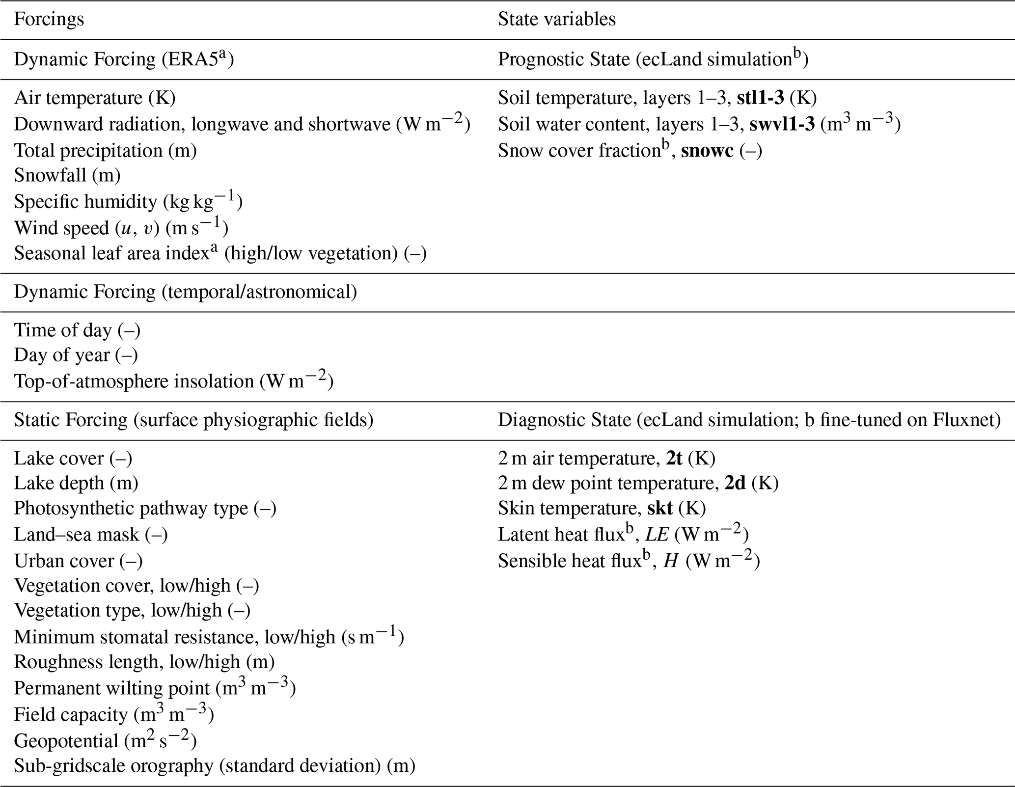
a From surface physiographic fields. b Diagnostic in ecLand.
2.1.1 ecLand
The ecLand model is the land surface component of the ECMWF Integrated Forecasting System (IFS) (Boussetta et al., 2021), building on the Carbon–Hydrology Tiled ECMWF Scheme for Surface Exchanges over Land (CHTESSEL; van den Hurk et al., 2000; Balsamo et al., 2009; Boussetta et al., 2013). It simulates the exchange of energy, water, and carbon between the land surface and the atmosphere, including associated subsurface processes. The model can be run either fully coupled within the IFS or in offline (uncoupled) mode forced by prescribed atmospheric fields.
Each grid box at the land–atmosphere interface is subdivided into surface tiles, with seven distinct classifications used over land: high and low vegetation, bare ground, shaded and exposed snow, intercepted water, lake, and urban. Each tile has its own physical parameters, allowing separate computation of water, heat, and momentum fluxes, and solution of an energy balance equation for tile skin temperature. Grid-box mean fluxes are obtained by area-weighted aggregation of tile-level fluxes and are passed to the atmospheric model.
For the ML emulator, we consider a subset of ecLand variables. In aiLand, soil water content and soil temperature in three layers (0–7, 7–28, and 28–100 cm) are treated as prognostic states, as in ecLand. Snow cover fraction is also treated as prognostic in aiLand, although in ecLand it is a diagnostic variable derived from the underlying prognostic snow water equivalent and snow density. Latent and sensible heat fluxes, 2 m air temperature, 2 m dew point temperature, and skin temperature are predicted as diagnostic outputs. In this study, ecLand CY49R2 (https://github.com/ecmwf-ifs/ecland, last access: May 2026) is run in offline mode, forced by ERA5 meteorological reanalysis (Hersbach et al., 2020). A global simulation covering 1998–2024 was performed at hourly temporal resolution on the native ERA5 Tco399 reduced Gaussian grid (∼31 km). Outputs were aggregated to 6-hourly time steps for training, to be consistent with that used in the AIFS.
2.1.2 Surface physiographic fields
Surface physiographic fields are assumed to be static and describe land surface characteristics such as orography, vegetation, soil type, land–sea mask, and surface albedo, capturing spatial heterogeneity relevant for land surface parameterisations. These fields determine the tile properties in ecLand and influence the computation of turbulent fluxes and tile skin temperatures. The fields are prescribed independently of model initial conditions. Leaf area index is provided using monthly climatologies to represent seasonal variability. All datasets are remapped to the model grid before use. In this study, physiographic fields derived from ERA5 (Hersbach et al., 2020) and their updated versions (Boussetta et al., 2021; Choulga et al., 2019; Muñoz-Sabater et al., 2021) are used, as described in Kimpson et al. (2023).
2.1.3 ERA5 reanalysis data
ERA5 is the fifth-generation atmospheric reanalysis produced by ECMWF (Hersbach et al., 2020). It is generated using IFS cycle 41R2 with 4D-Var data assimilation for the atmosphere, a land data assimilation system (de Rosnay et al., 2022), and a coupled land-atmosphere modelling approach using ecLand (Boussetta et al., 2021). ERA5 provides hourly atmospheric and surface fields at approximately 31 km horizontal resolution with 137 vertical levels extending to 80 km height. Uncertainty estimates are available at ∼63 km resolution from a 10-member ensemble. In this study, hourly ERA5 surface fields at ∼31 km resolution on the cubic octahedral reduced Gaussian grid (Tco399; N320) are used as dynamic forcing inputs.
2.1.4 Fluxnet observations
Flux-tower measurements from the FLUXNET network (Baldocchi et al., 2001; Pastorello et al., 2020) provide in situ observations of land–atmosphere exchanges of energy, water, and carbon based on the eddy covariance technique. These observations include turbulent fluxes such as latent heat (LE) and sensible heat (H), together with meteorological drivers (e.g., radiation, air temperature, and precipitation) typically measured at half-hourly resolution.
In this study, we use the harmonised flux tower dataset provided by FluxDataKit (Hufkens and Stocker, 2025), which compiles and standardises observations from several openly available flux data products including PLUMBER-2 (Abramowitz et al., 2024), AmeriFlux (Novick et al., 2018), and ICOS releases (e.g., Warm Warm Winter 2020 Team and ICOS Ecosystem Thematic Centre, 2022). The dataset provides quality-controlled and gap-filled fluxes and meteorological variables with consistent formatting across sites, as well as site metadata and continuous multi-year records suitable for model calibration and benchmarking. We use FluxDataKit's energy-balance-closed variant of the turbulent fluxes, in which raw H and LE are scaled proportionally to satisfy at each timestep (where Rn is net radiation and G is ground (soil) heat flux). This follows standard FLUXNET2015 conventions and removes the well-documented systematic underestimation of turbulent fluxes by raw eddy-covariance measurements (Wilson et al., 2002; Stoy et al., 2013) and preserves the observed Bowen ratio at each site.
The observational dataset is split into training and validation subsets (see Appendix B), ensuring spatial separation between training and evaluation periods. For the fine-tuning part of this study, we train the model over the years 2000–2019 for 199 calibration sites, retaining 42 validation sites to also be evaluated over this period. For the main evaluation, the validation period of 2020–2023 was used, at the 84 training and 17 validation sites with valid post-2020 FLUXNET data. All metrics are computed on daily means, only where both prediction and observation are non-missing.
2.1.5 Data preprocessing
All datasets are prepared using the anemoi-datasets framework (https://anemoi.ecmwf.int/, last access: 10 November 2026) and stored in Zarr format, chunked in time to optimise input/output (I/O) performance. Dataset generation is controlled via YAML-based recipe files to ensure reproducibility. Feature-wise statistics (mean and standard deviation) are computed over the ecLand training period as part of the dataset creation pipeline and stored for subsequent use during model training.
The final dataset used for model pretraining comprises global ecLand simulations and ERA5 reanalysis time series for 1998–2024 at 6-hourly temporal resolution, together with static surface physiographic fields, defined on the model grid (N320, 171039 land points). Of this period, 1998–2019 is used for pretraining, 2022 for validation, and 2020–2023 is withheld for out-of-sample evaluation (Sect. 2.2.4); the evaluation window ends in 2023 to match the availability of FLUXNET observations. Two separate observational datasets are created for training and validation for the fine-tuning step, covering 199 and 42 sites respectively, reducing the spatial dimension compared to the full model grid. FLUXNET observations (or missing values) replace model-derived surface fluxes, while other prognostic and diagnostic variables are retained from the simulations.
2.2 Machine learning model
In preliminary experiments (Wesselkamp et al., 2025), several ML models were tested to emulate ecLand, including LSTM (Long-Short Term Memory, Hochreiter and Schmidhuber, 1997), XGB (eXtreme-Gradient Boosting, Chen et al., 2015), and MLP (Multi-Layer Preceptor, as described in Goodfellow et al., 2016). While the LSTM excelled in long-range forecasts of soil temperature and snow cover, and XGB was robust for soil moisture, the MLP offered a favourable balance between accuracy and computational efficiency. For this study, we have expanded the scope of the MLP, including refined hyperparameters, longer rollouts, an extended input space (adding temporal and astronomical forcings shown to improve soil temperature predictions), and a set diagnostic outputs, building substantially on the prototype introduced in Wesselkamp et al. (2025).
2.2.1 Model architecture
The MLP emulator is a feed-forward neural network approximating ecLand’s mapping from static, dynamic, and prognostic inputs to land surface states and fluxes:
Here, the input vector x∈𝒳 consists of static, dynamic, and prognostic state variables, while the output vector y∈𝒴 contains prognostic state variable increments and diagnostic variables at the next timestep. The true mapping f is approximated by a learned function f*(x) via stochastic gradient-based optimisation.
The network comprises a shared prognostic backbone that produces a latent representation, which is projected to prognostic targets, and a diagnostic branch that combines climatological, meteorological, and prognostic information to predict diagnostic variables. Prognostic outputs are applied in a residual formulation, where predicted increments are added to the previous state, enabling stable autoregressive rollouts. Diagnostic variables are predicted as absolute values without memory of their previous value, mirroring ecLand, where skin temperature and the turbulent fluxes are computed from the tile energy balance at each time step rather than carried over from the previous one as prognostic states. Post-processing enforces variable-specific physical bounds. Physical consistency is therefore inherited from the ecLand training target and reinforced by the residual formulation and output bounds, rather than imposed through conservation laws or physical penalties within the network (see Sect. 4.3 for details).
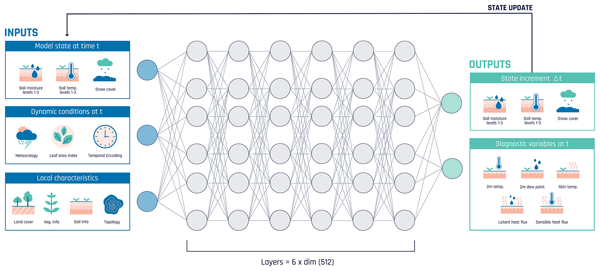
Each hidden layer applies a fully connected (linear) transformation, followed by layer normalisation (Ba et al., 2016), followed by a rectified linear unit (ReLU) activation. Layer normalisation standardises each sample's activations across the feature dimension, stabilising training and reducing sensitivity to the differing scales of the input variables; ReLU introduces the non-linearity needed to capture ecLand's non-linear input–state mapping. The base model uses six hidden layers of width 512, with approximately 1.3 M trainable parameters, and a single-block diagnostic head. Figure 1 illustrates the architecture. Note that this model is wider and deeper than the version presented in Wesselkamp et al. (2025) to account for the additional variables.
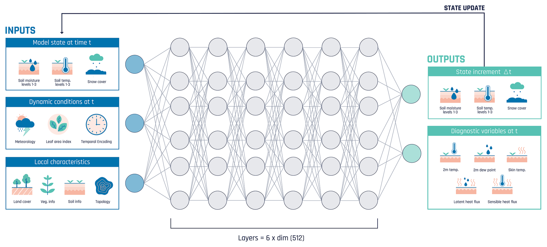
Figure 1Schematic of the MLP emulator architecture, showing the shared prognostic backbone and diagnostic branch.
2.2.2 Loss function
The model is trained using a smooth L1 loss (Huber loss with β=1). Loss is accumulated across the autoregressive rollout: errors at each forecast step are summed and then scaled by the inverse rollout length. Global weights balance prognostic and diagnostic contributions, with optional per-variable weighting for individual targets (here all set to 1); when per-variable weights are used, the weighted losses are averaged over the number of variables. Prognostic increments are normalised before the loss by dividing by tendency scalers – the standard deviation of 6-hourly increments over the training set – ensuring balanced contributions across variables with different characteristic evolution rates. Diagnostic variables, which are standardised like all other targets, receive no additional tendency scaling since they are predicted as absolute values rather than increments. During fine-tuning to observations, the loss is computed only over valid (non-NaN) target elements, allowing the model to learn from sparse observational datasets where only a subset of variables or grid points carry valid values at any given time. Input features (meteorological forcing, prognostic states, and static physiographic fields) are sourced from the complete ERA5 reanalysis and ecLand simulations, which do not contain missing values at valid land grid points; a residual safety guard replaces any unexpected NaN in inputs with zero in normalised space.
2.2.3 Training strategy
Pretraining uses global ecLand simulations at N320 resolution from 1998–2019 (approximately 32 000 six-hourly timesteps over 171 039 land points), with 2022 reserved for validation and checkpoint selection. The years 2020–2023 are excluded from training and used exclusively for out-of-sample evaluation (Sects. 3.1.1 and 3.2). Input features are normalised using feature-wise statistics computed over the full dataset, with variable-specific schemes (e.g., standardisation, max-scaling, or identity for categorical inputs). Missing values are masked during loss computation and set to zero in inputs.
Training proceeds in two phases with increasing rollout horizon. In Phase 1, the model is trained for 80 epochs (160 000 steps) with rollout length R=4 (24 h). The Adam optimiser is used with a peak learning rate of , decayed to using a cosine schedule with 1000-step linear warmup. In Phase 2, the best checkpoint is fine-tuned with rollout R=8 (48 h) for 8 epochs (16 000 steps) at a reduced learning rate of . Gradient clipping (global norm 5.0) is applied throughout, and gradient checkpointing is enabled for longer rollouts to manage memory.
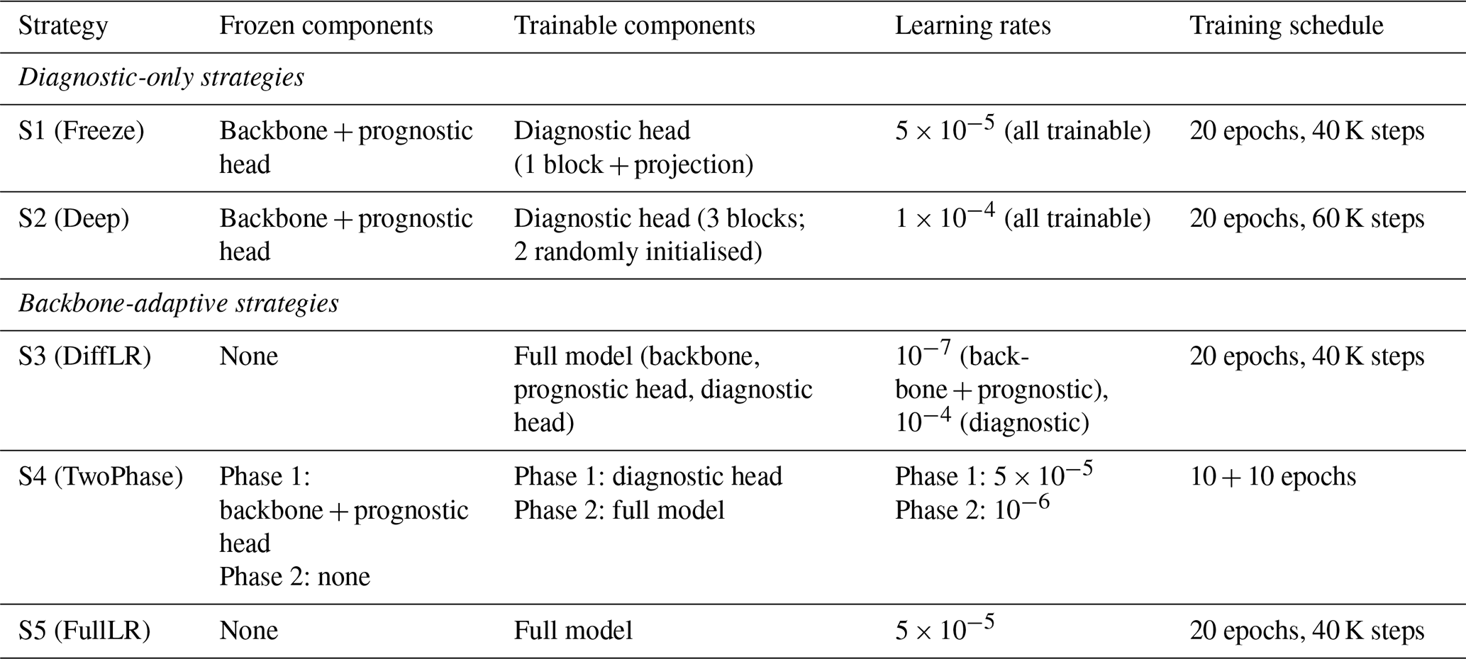
Each training step processes one sample, defined as a rollout window of R consecutive 6-hourly timesteps spanning all valid land grid points (171 039 for global pretraining; 199 for FLUXNET fine-tuning). Training is performed on 4 GPUs using distributed data parallelism with mixed precision, giving an effective batch of 4 rollout windows per gradient update. The smaller effective batch during fine-tuning (constrained by FLUXNET data volume) interacts with the choice of low fine-tuning learning rates: the very low rates used (10−5 to 10−7, Table 2) help mitigate noise from small batches, but rigorous separation of batch-size effects from data-distribution effects on fine-tuning quality would require a dedicated ablation study, which we defer to future work. The best checkpoint is selected based on validation loss.
2.2.4 Fine-tuning on observations
For the second part of this study, we fine-tune the aiLand-base emulator using in situ flux data. The observational data are normalised using the same statistics as during pretraining for consistency. We investigate five fine-tuning strategies (Table 2) spanning a methodological spectrum from minimum-intervention to full-model adaptation, designed to test how aggressively the pretrained backbone should be modified during fine-tuning. Higher backbone learning rates risk catastrophic forgetting of the pretrained dynamics, while overly low rates limit fine-tuning's ability to correct inherited LSM biases; the five strategies span this trade-off. Diagnostic-only strategies (S1, S2) freeze the prognostic backbone entirely and update only the diagnostic head, ensuring that the state dynamics learned from ecLand pretraining are preserved exactly. S2 tests whether additional learning capacity in the diagnostic head improves flux predictions, by extending it to 3 blocks (two randomly initialised) before fine-tuning. Backbone-adaptive strategies (S3, S4, S5) update the prognostic backbone at a substantially lower learning rate than the diagnostic head, allowing gradual adaptation while protecting the pretrained dynamics. S3 uses a single training phase with explicit differential learning rates (backbone 10−7, diagnostic 10−4). S4 adopts a two-phase procedure: first updating only the diagnostic head, then unfreezing the full model at a uniform low learning rate (10−6) to mitigate catastrophic forgetting. S5 updates the full model from the start with a uniform learning rate () across all components.
2.3 Evaluation tools and metrics
2.3.1 Standard metrics
To evaluate model performance, we use common metrics such as the root-mean-square error (RMSE), the mean absolute error (MAE) and the anomaly correlation coefficient (ACC). The ACC is calculated as the Pearson correlation between predicted and reference anomalies, defined as deviations from the climatology. The climatology is computed from the ecLand dataset over a multi-year reference period (here 1998–2024) using a sliding-window approach. For each 6-hourly timestep, samples are assigned to their hour-of-year bin and to neighbouring bins within a ±3 d window (cyclically), and averaged across all years to obtain a smoothed climatological mean for each timestep, variable, and grid point. All metrics are on the N320 reduced Gaussian grid, with glacier and coastal points excluded throughout.
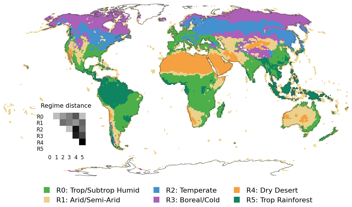
Figure 2Global distribution of regime classes. Each grid cell is assigned to one of six regime categories. The panel in the bottom left-hand corner shows the Euclidean distance between cluster centroids.
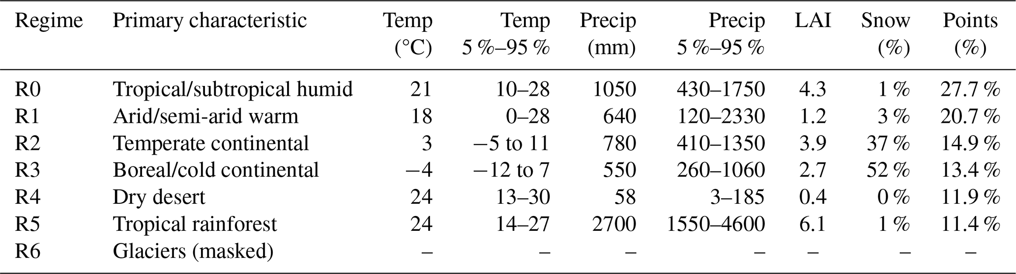
Table 3Primary characteristics of the different regimes. The provided ranges are the 5th–95th percentiles of the grid-point distribution of climatological means within each regime. Descriptive names are interpretive labels for the dominant character of each cluster and do not correspond to established biome or climate classes (overlaps with Köppen–Geiger group are given in Table A1).
2.3.2 Climate–land-surface regimes
To test the transferability of aiLand-base, we partitioned the land surface into climate–land–surface regimes by clustering those in a feature space that combines climatological indicators with land-surface states (soil moisture, snow cover, Bowen ratio). Working in a metric feature space lets us relate transfer skill to the distance between regimes, and test whether a single global model matches regime specialists, both on regimes it has seen and on one withheld from training. Climatological features (2009–2020) were computed from ERA5, including monthly mean and seasonal amplitude of 2 m temperature and precipitation, aridity index, top-layer soil moisture, snow cover fraction, leaf area index (LAI), and Bowen ratio. The features define static spatial regions, so a decade-long window suffices; computing them over the full training period instead assigns 98.9 % of land points to the same regime, which does not provide a justifiable improvement over the shorter period. All features were standardised to zero mean and unit variance prior to analysis to ensure comparable contributions across variables with different units. Regimes were identified using k-means clustering (Lloyd, 1982). The number of clusters was chosen by evaluating three cluster validity metrics over k=2–12: the silhouette score (Rousseeuw, 1987), the Davies–Bouldin index (Davies and Bouldin, 1979) and the Calinski–Harabasz index (Caliński and Harabasz, 1974). The first two are optimised at k=7, which lies within 1.3 % of the optimum of the third at k=9; we therefore use k=7. One cluster predominantly corresponding to glaciated or ice-covered regions was masked prior to transfer experiments, leaving six effective regimes. Spatial coherence of the regime labels was enforced using a local majority filter to suppress isolated cells while preserving large-scale structure.
We interpret the resulting clusters as climate-vegetation regimes (summarised in Fig. 2 and Table 3). The six-cluster partition captures broad climate-vegetation regimes rather than following the usual regime naming conventions: “temperate continental” includes both grasslands and forests with similar climates, and “tropical/subtropical humid” is distinguished from “tropical rainforest” by precipitation and LAI rather than by latitude. The arid/semi-arid and dry-desert clusters are separated by an order-of-magnitude difference in mean precipitation (640 mm yr−1 vs. 58 mm yr−1) and vegetation cover (LAI 1.2 vs. 0.4), reflecting genuinely different surface energy and water budgets. However, the regime are not internally homogeneous: hard k-means clustering of continuous climate features inevitably assigns transition-zone grid points to single clusters despite genuinely intermediate characteristics. An internal margin analysis (relative distance to nearest vs. second-nearest centroid) indicates that around 30 % of all grid points fall in transition zones (borderline assignments or grid points reassigned by the spatial-coherence filter). The dry desert cluster (R4) is the most internally consistent, with only 11 % of its grid points in transition zones, while the tropical/subtropical humid cluster (R0) is the most heterogeneous (40 % transition-zone cells). Cross-regime transfer experiments (Sect. 3.1.3) should therefore be interpreted as testing transferability across overlapping climate regimes rather than cleanly separated ecosystems.
For each regime, we extract latitude/longitude coordinates to define training subsets. Pairwise Euclidean distances between cluster centroids in feature space are computed to quantify regime similarity for these transferability analyses. Each specialist and the global model is evaluated on every regime, with RMSE normalised per variable by the mean in-regime specialist RMSE, so that 1.0 corresponds to average specialist skill. The transfer penalty of a model on a regime is its normalised RMSE there relative to that of the regime's own specialist, minus one.
3.1 aiLand-base performance
For the first part of the results, we evaluate how well the aiLand-base emulator reproduces ecLand and how robust it is across lead times, multi-year integrations, ecosystem regimes, and spatial resolutions. A recurring finding is that prognostic state variables 00 predicted via a residual increment formulation – generalise cleanly, because the increment is small relative to the absolute state and is tightly anchored to the previous timestep, whereas diagnostic variables – predicted as absolute values at each step – are more sensitive to regime and resolution. We establish this asymmetry in the lead-time and stability analysis, then show that it defines the error structure across regimes and grids.
3.1.1 Overall performance and stability
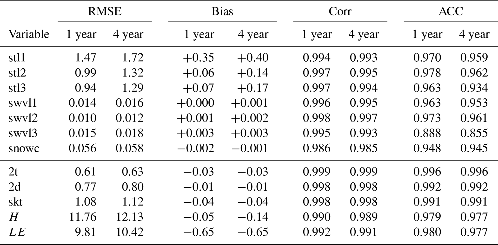
We evaluate aiLand-base in two complementary protocols, both forced by ERA5 atmospheric reanalysis (the same forcing used in the corresponding ecLand simulations) and both initialised from ecLand state at the start time. The first protocol consists of 138 independent 90 d integrations launched every two days from January through early October 2022 (the latest start date allowing a full 90 d window within the evaluation year), used to characterise short- to sub-seasonal error growth as aiLand-base departs from ecLand when both are initialised from the same state and driven by identical forcing (Table 4, Fig. 3a). The second consists of continuous autoregressive integrations over 2020 (1 year) and 2020–2023 (4 year), used to assess long-range stability and the representation of the seasonal cycle (Table 5, Fig. 3b).
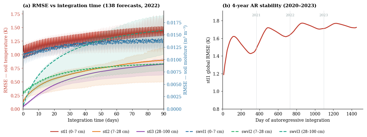
Figure 3Skill of the emulator for soil temperature (solid lines, left axis) and soil moisture (dashed lines, right axis) at three depth layers, both panels using ERA5-forced offline integrations of aiLand-base. (a) Global RMSE as a function of integration time, averaged over 138 independent 90 d integrations initialised every two days from ecLand state throughout 2022; shading shows the interquartile range across integrations. (b) Global stl1 RMSE during a continuous 4-year autoregressive integration initialised on 1 January 2020 from ecLand state.
Table 4Global RMSE of aiLand-base against ecLand by integration time, averaged over 138 ERA5-forced 90 d integrations initialised throughout 2022. The final column gives the 1 to 90 d growth ratio. Surface heat flux values (H, LE) are reported as RMSE of the time-averaged flux in W m−2 over each 6-hourly timestep. RMSE magnitudes and growth ratios should be interpreted within each variable class rather than across, since native units and dynamic ranges differ (e.g. thermal vs. hydrological).
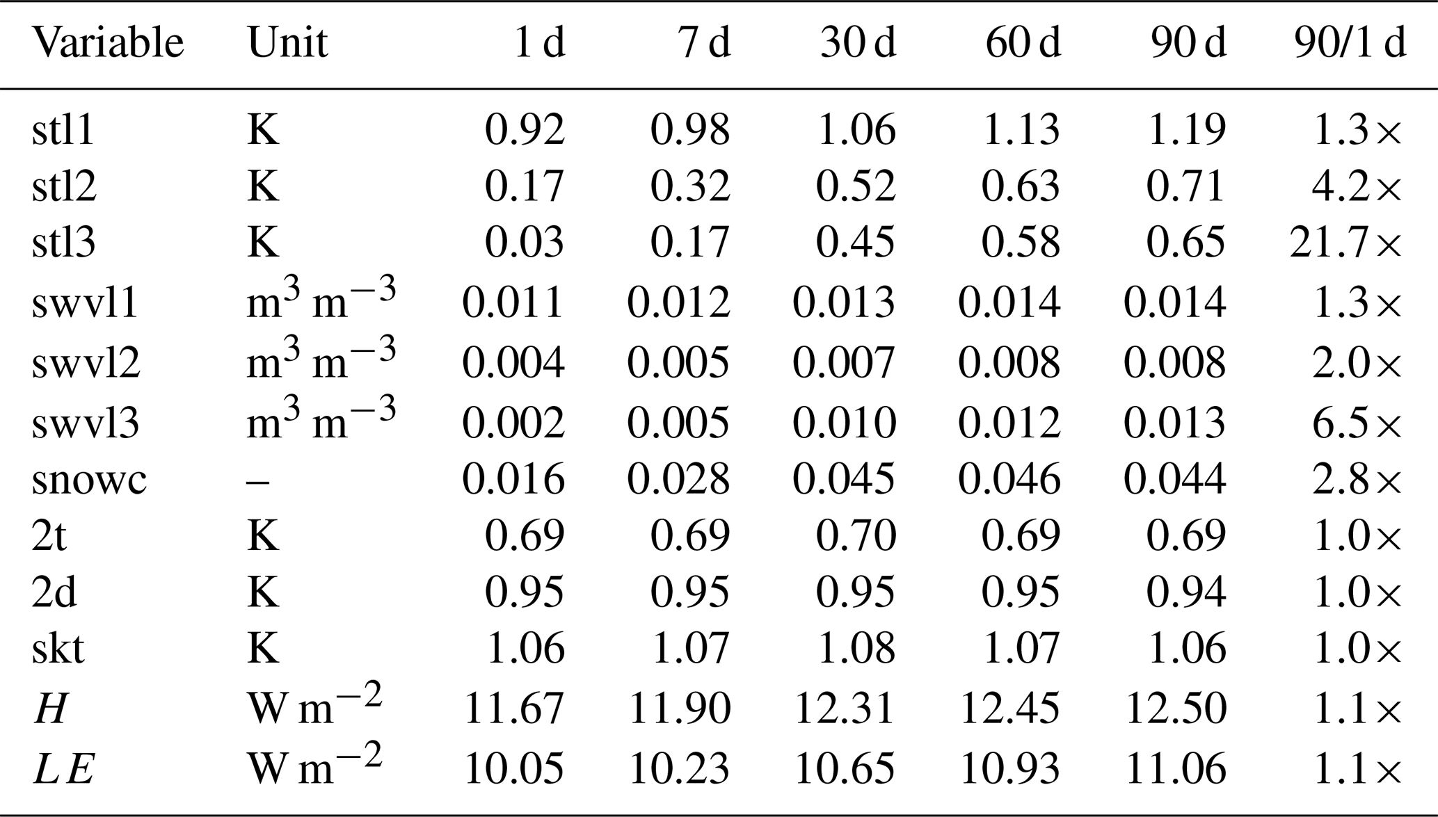
Table 5Global metrics from continuous autoregressive integrations over 2020 (1 year) and 2020–2023 (4 year, approximately 5800 time steps). Surface heat flux values (H, LE) are reported as RMSE and bias of the time-averaged flux in W m−2 over each 6-hourly timestep.
Errors remain well controlled over the 90 d integration horizon (Table 4, Fig. 3a). Surface soil temperature (stl1) RMSE rises by 29 % and surface soil moisture (swvl1) by 19 %. Deep soil layers have very small day-1 errors (stl3: 0.03 K; swvl3: 0.002 m3 m−3), reflecting long memory timescales, so their apparent growth ratios are large (stl3: 21.7×) despite absolute errors remaining smaller than at the surface throughout the time integration. Unlike the surface layer, where errors are continually corrected by the forcing, deep-layer increments depend mostly on the state itself, so errors there accumulate rather than being corrected. Snow cover RMSE peaks at intermediate lead times (0.046 at 60 d) before declining slightly, consistent with transition-season timing errors rather than monotonic drift. Diagnostic variables (2 m temperature: 0.69 K; skin temperature: 1.06 K; sensible heat flux: 11.7–12.5 W m−2; latent heat flux: 10.1–11.1 W m−2) show near-constant RMSE across all lead times, confirming that they are effectively re-diagnosed from the prognostic state at each step rather than accumulating error.
This stability is confirmed over continuous integration (Table 5). While stl1 RMSE gradually increases from 1.47 K (1 year) to 1.72 K (4 year), a 17 % increase, and stl2 and stl3 grow by 34 % and 37 %, respectively, correlation coefficients remain high across all soil variables (≥0.993 for temperature; ≥0.993 for moisture), and anomaly correlations stay above 0.93 for all prognostic variables except swvl3, which decreases from 0.888 to 0.855. The stl1 RMSE trace (Fig. 3b) shows a seasonal cycle but no upward trend, confirming stable autoregressive behaviour with no dynamical divergence. Soil moisture RMSE grows more slowly than temperature (14 %–20 % over four years), and snow cover is nearly stable (+4 %), indicating negligible drift in non-thermal prognostic variables. Diagnostic variables degrade minimally (2 m temperature: 0.61 to 0.63 K; sensible heat flux: 11.8 to 12.1 W m−2; latent heat flux: 9.8 to 10.4 W m−2), with correlations remaining near unity (∼0.998–0.999) and anomaly correlations above 0.99.
The dominant systematic feature is a +0.40 K warm bias in stl1, present at 89 % of land grid points and largely established within the first year of integration. Equivalent integrations within the training period yield comparable biases (+0.44 to +0.47 K), confirming that the offset is an intrinsic property of the learned dynamics rather than distribution shift. The bias is consistent with a conditional-mean offset induced by the Smooth L1 loss under the right-skewed soil-temperature increment distribution (training skewness +0.94), with an additional Arctic component reflecting underestimated polar warming. The skew weakens with depth (0.42 for stl2, and approximately zero for stl3 once the most extreme 1 % of grid points is excluded), consistent with the bias being largest in the surface layer, which receives the diurnal forcing directly. The bias confined to soil thermal variables; moisture biases are negligible and diagnostic temperatures show small negative offsets consistent with per-step re-diagnosis.
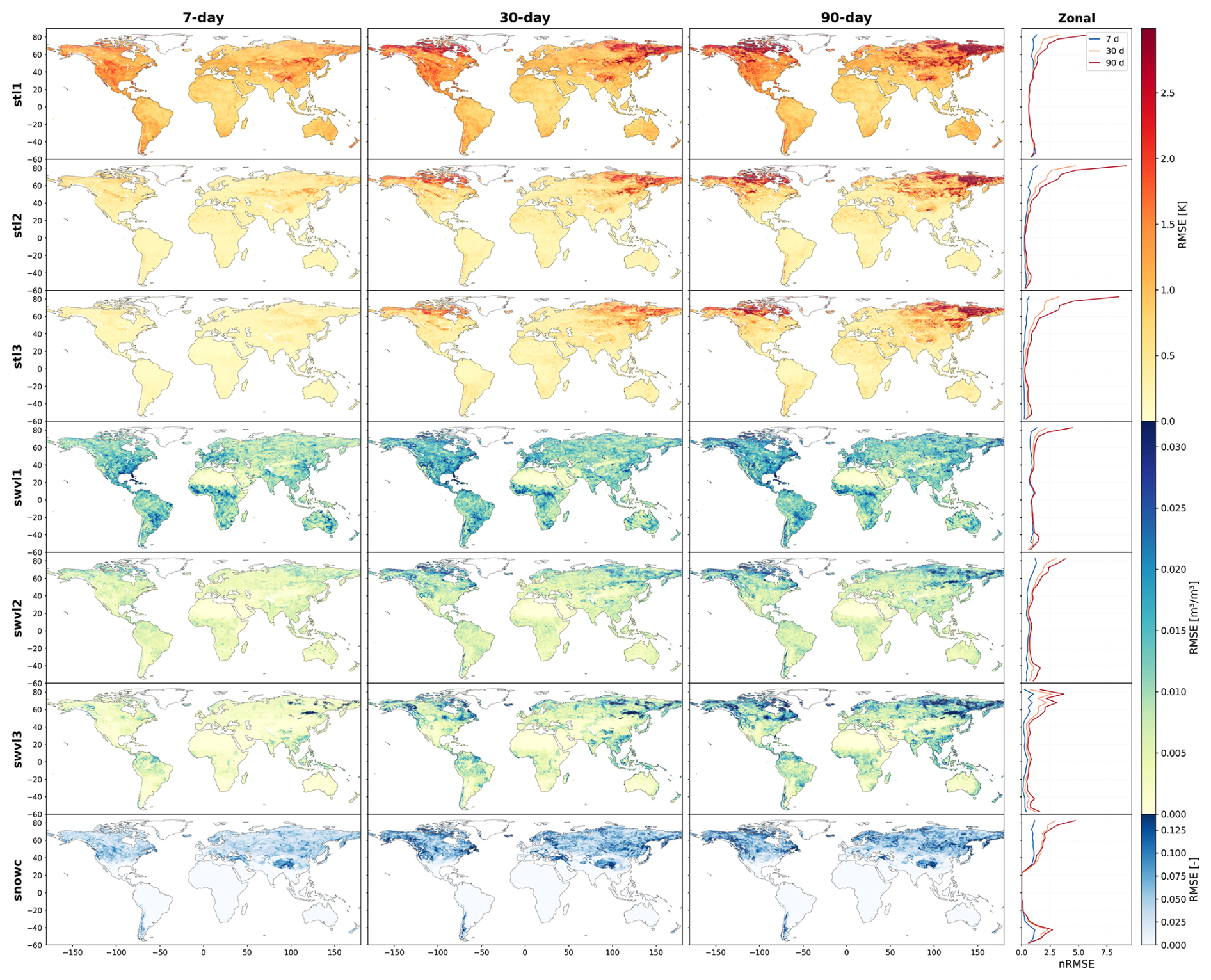
Figure 4Spatial distribution of prognostic RMSE at 7, 30, and 90 d integration times (columns 1–3), with normalised zonal profiles (column 4). Each row shows one prognostic variable: soil temperature (stl1-3), soil moisture (swvl1-3), and snow cover (snowc). Zonal profiles are normalised by each variable's global RMSE at 90 d integration time.
3.1.2 Error structure and the role of snow cover
The global RMSE values in Sect. 3.1.1 mask strong geographic structures (Fig. 4). At latitudes >60° N the 90 d RMSE reaches 2.42 K for stl1 and 0.018 m3 m−3 for swvl1 – roughly three times its tropical value. The soil moisture comparison is harder to interpret directly because hydraulic properties and dynamic ranges differ between regions, and freezing affects the modelled state in cold winters; we therefore focus the analysis on relative spatial patterns rather than absolute magnitudes. A spatial decomposition (Fig. 5a) shows that the high-latitude error amplification is dominated by seasonal snow cover, although freeze-thaw cycling and reduced atmospheric coupling in cold winters likely contribute as well. Grid points with seasonal snow (fractional snow-cover RMSE > 0.02; 33 % of valid land area) account for 57 %, 82 %, and 76 % of the global stl1, stl2, and stl3 mean squared error at 90-day integration time. In these zones stl1 RMSE is 1.83 K (2.1× the snow-free value), stl2 is 1.31 K (4.3×), and stl3 is 1.16 K (3.5×); swvl3 is 2.9× the snow-free value. Seasonal snow covers 95 % of all land poleward of 60° N and 62 % of the 30–60° N band but less than 1 % of the tropics, explaining the latitudinal error gradient.
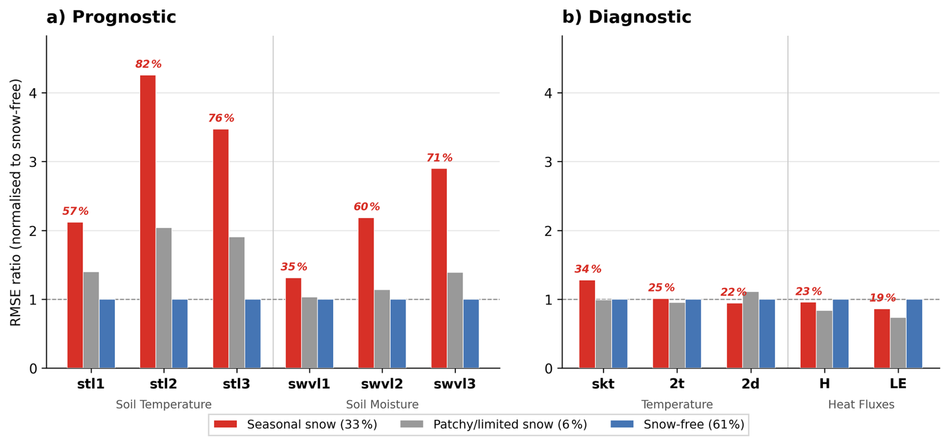
Figure 5RMSE by snow regime at 90 d integration time, normalised by the snow-free baseline. Land grid points are classified by their 90 d snow cover RMSE into seasonal-snow (snowc RMSE > 0.02, 33 % of land; red), patch/limited snow (0.005–0.02, 6 %; gray), and snow-free (<0.005, 61 %; blue) regimes. Bars show RMSE for soil temperature (a, K) and soil moisture (b, m3 m−3) in panel (a) and diagnostics in panel (b). Italic red numbers show the percentage of global MSE contributed by seasonal-snow zones.
Consistent with the diagnostic re-diagnosis pathway established above, diagnostic outputs are largely unaffected by snow regime (Fig. 5b): 2 m temperature RMSE is nearly identical across regimes (0.70 K vs. 0.69 K snow-free), and surface heat fluxes are actually lower under snow cover. This is physically expected: snow's high albedo and the frozen surface state both suppress the absolute magnitude of turbulent exchange, so absolute flux errors are smaller in snow-covered conditions. Only skin temperature shows mild amplification (1.3×), reflecting its direct coupling to the prognostic soil state.
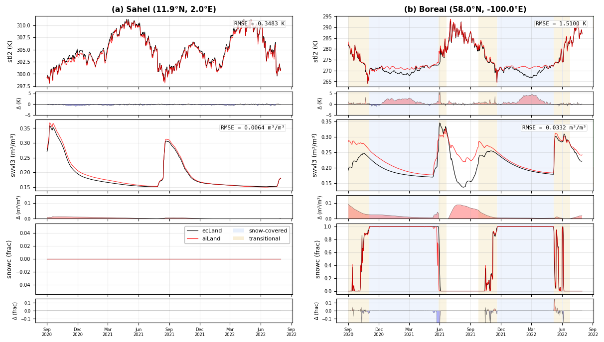
Figure 6Point-level time series at a snow-free site (Sahel, 13.5° N; a) and a boreal site with seasonal snow cover (60.5° N; b) from a continuous 4-year autoregressive run (September 2020–August 2022 shown). Rows show soil temperature at layer 2 (stl2), soil moisture at layer 3 (swvl3), and snow cover fraction, each with a residual strip (aiLand-base – ecLand) below. Blue shading marks snow-covered periods (snow cover ≥ 0.99); yellow shading marks transitional periods (fractional snow cover ± 5 d buffer).
Error seasonality at snow-affected sites differs sharply between thermal and hydrological variables, as illustrated by point-level traces from the continuous 4-year integration (Fig. 6). At a representative warm arid site (Fig. 6a), aiLand-base tracks ecLand essentially perfectly year-round, confirming that the residual errors identified above are regime-specific rather than systematic. At the boreal site (Fig. 6b), soil temperature errors concentrate during sustained snow cover rather than at onset or melt transitions: stl2 RMSE under continuous snow is 1.71 K vs. 0.37 K in snow-free months (4.6×). Snow acts as an insulating layer that decouples the soil column from atmospheric forcing, weakening the learned mapping from meteorological inputs to soil-state increments; sub-surface variables are disproportionately affected because they are furthest from any remaining surface coupling. Soil moisture exhibits the opposite seasonality: swvl1–3 errors peak after the snow has gone, during the active hydrological season when freeze-thaw cycling and snowmelt-driven rewetting produce complex transient dynamics that are harder for the emulator to track. Under snow cover itself, by contrast, soil moisture is largely frozen and temporally static, so low variability yields low error.
This site-level contrast generalises to the global error field. Grid points with seasonal snow show soil moisture RMSE 1.3–2.7× higher than permanently snow-free regions, and 85 % of snow-zone grid points exceed the snow-free median despite the errors occurring primarily outside the snow-covered season. Insulation and freeze–thaw mechanisms therefore act on different variables and in different seasons, but both have a strong impact on the annual error budget of snow-affected regions. Future work could improve this regime by extending the emulator to predict surface and sub-surface runoff, allowing it to better account for snowmelt routing and the post-melt soil-moisture dynamics.
3.1.3 Cross-regime robustness
A key question for ML-based land surface emulators is whether learned input-output mappings remain valid across climate-land-surface regimes, including extreme climates not well sampled during training. The snow-coupling analysis above predicts that cold-climate regimes should be among the hardest targets, because specialists trained on narrow climate regimes will not encounter enough snow-insulated soil dynamics to learn the distinct forcing-state relationship that applies under a snowpack. To test this and to evaluate broader regime sensitivity, we trained six regime-specialist models on data-driven clusters (see Table 3 and Fig. 2 for full characterisation). Each specialist was evaluated within its home regime and across all others (Fig. 7a), alongside the globally trained model evaluated under the same protocol.
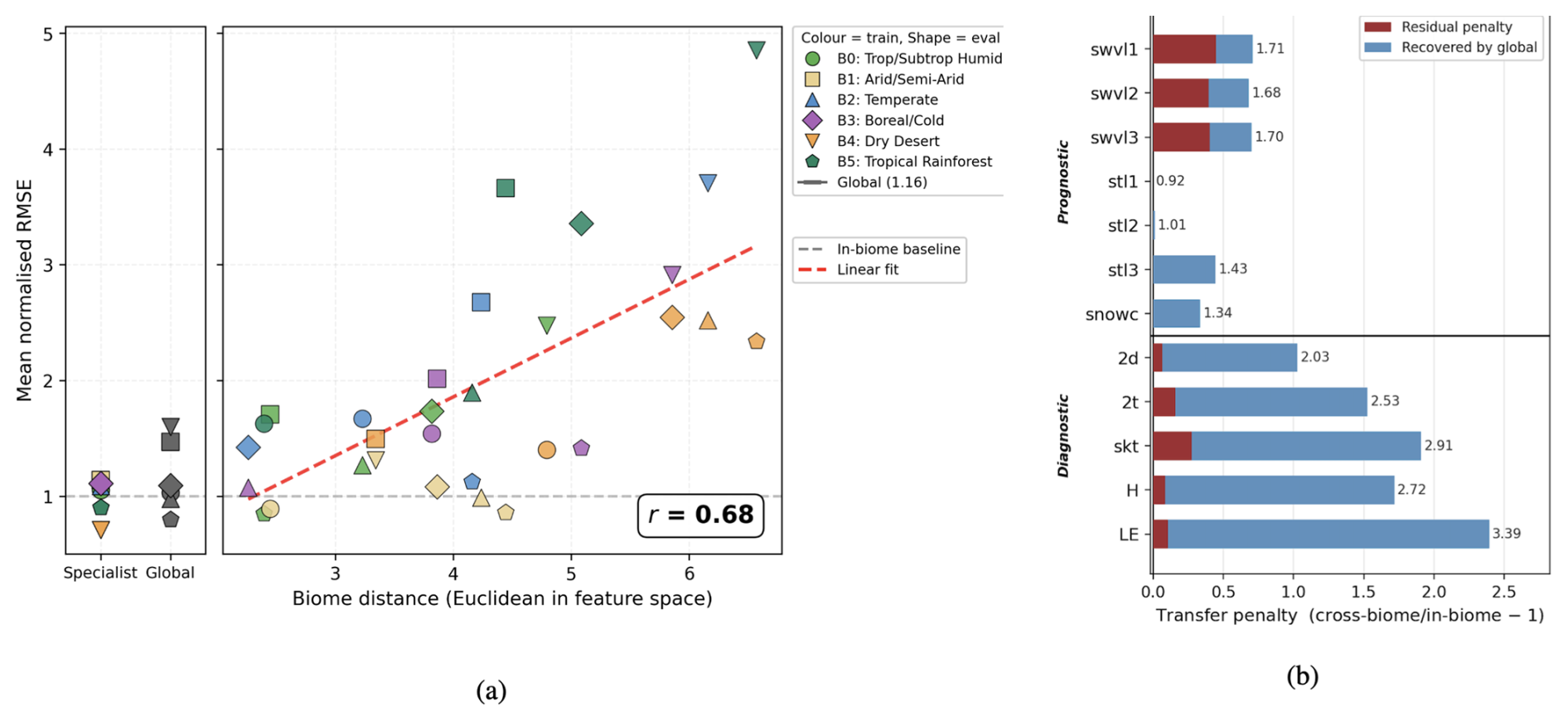
Figure 7Cross-regime transfer skill. (a) In-regime specialist performance (a; coloured markers) and the global model (grey) evaluated on each regime, alongside cross-regime transfer penalty as a function of regime dissimilarity (b). Each point represents a specialist trained on one regime and evaluated on another; marker colour indicates training regime, marker shape the evaluation regime. The R5 → R4 point (tropical rainforest model evaluated on desert) is annotated; all points evaluated on R4 are outlined to highlight the desert-as-target cluster. RMSE is normalised by the mean in-regime specialist RMSE (averaged across all 12 output variables), so 1.0 corresponds to average specialist performance (dashed line). (b) Mean transfer penalty per variable (Sect. 2.3.2) of specialists applied outside their training regime. The red portion is the penalty the global model still incurs on the same regimes (residual penalty); the blue portion is the difference (recovered by global training). Numbers give the total cross-regime RMSE ratio (penalty + 1).
Regimes are not uniformly learnable (Fig. 7a, left panel). R4 and R5 are the most easily fitted by their respective specialists, reflecting their relatively clean cluster definitions (R4: only 11 % transition-zone cells; R5: 24 %; see Sect. 2.3.2). R2 and R3 show above-average in-regime errors reflecting a combination of greater internal process heterogeneity and substantial transition-zone content (∼26 %–28 %). Against this in-regime baseline, transfer penalty scales with dissimilarity in the training feature space (r=0.68; Fig. 7a, right panel). Transfers between similar regimes remain close to parity, while extreme shifts degrade strongly: R5 to R4 transfer reaches 4.9× the in-regime baseline. R4 emerges as the most challenging target overall (mean 3.1×), consistent with its outlier climatology (Table 3): on the precipitation axis it overlaps only with R1, so transfers into it are extrapolations for every other specialist, whereas R1, spanning 120–2330 mm, overlaps both R4 and R0. The R4 penalty is partly amplified by near-zero in-regime variability for several variables.
The globally trained model achieves a mean normalised RMSE of 1.16; only 16 % above the specialist in-regime baseline. Its largest penalties occur in dry regimes (1.47 for R1; 1.60 for R4), reflecting different mechanisms in each case. R1 makes up 21% of land grid points (not under-sampled) but has substantial transition-zone content (∼31 % borderline or reassigned cells; Sect. 2.3.2), so its representation is diluted into neighbouring clusters during global training. R4 is internally consistent (only 11 % transition-zone cells) but combines outlier climatology (58 mm yr−1 precipitation vs. 550–2700 in other regimes, LAI 0.4 vs. 1.2–6.1) with a small sample share (12 % of land points), so the global training distribution provides limited explicit coverage of its distinctive surface energy and water budget. Notably, the global model outperforms cross-regime specialist transfers for the temperate (R2) and rainforest (R5) regimes. These are regimes where the specialists themselves face challenging training distributions: R2 spans grasslands and forests with similar climates but distinct surface physics, and R5 cells appear partly in R0 due to the continuous precipitation-LAI gradient (Sect. 2.3.2). The global model benefits from having seen the full climate continuum without enforced cluster boundaries.
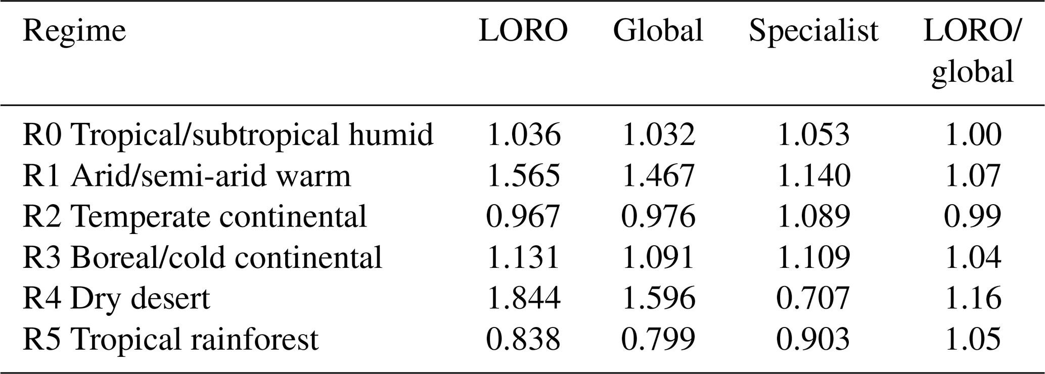
Because the global model has seen every regime in training, its advantage over cross-regime specialist transfer could reflect exposure rather than generalisation. To separate the two, six leave-one-regime-out models were trained on all regimes but one and evaluated on the held-out regime (Table 6). Removing a regime degrades performance on it only slightly: four of six regimes are within 5 % of the global model, and the largest degradation is 16 % for R4, against cross-regime specialist penalties reaching 4.9×. The cost of omitting a regime does not scale with its share of the training data: removing R0, the largest regime in Table 3, has no effect, whereas removing R4, one of the smallest, is the most damaging. What matters is whether the remaining regimes contain the same physical conditions; R1 and R4 are the only water-limited regimes in the partition, so removing either removes most of the exposure to soil-moisture-limited evaporation.
Table 6Leave-one-regime-out (LORO) performance. Each LORO model is trained on all regimes but the target and evaluated on the held-out regime. RMSE is normalised by the mean in-regime specialist RMSE; global and in-regime specialist values are reproduced from Fig. 7a. Single training runs, so differences of a few per cent are within run-to-run variations.
The prognostic-diagnostic asymmetry identified in Sect. 3.1.2 persists across regimes (Fig. 7b). Prognostic variables incur moderate transfer penalties (mean ratios 0.92–0.71), with soil temperature layers transferring almost perfectly (stl1: 0.92; stl2: 1.01) and soil moisture and snow cover showing larger penalties (1.34–1.71). Diagnostic variables are substantially more sensitive (median 2.0× vs. 1.1× for prognostics), with latent heat flux (3.4×) and skin temperature (2.9×) the most affected. The stacked decomposition in Fig. 7b shows that global training recovers the majority of the diagnostic cross-regime penalty, indicating that training over diverse climate samples largely compensates for regime-specific surface-atmosphere coupling.
Overall, a single global model provides the most robust performance across regimes, and this is not simply because it has seen every regime in training: removing a regime degrades performance on it by at most 16 %, against transfer penalties of up to 4.9× when a specialist is applied outside its training regime. What the global model gains is exposure to conditions (e.g., water limitation, snow-insulated soil) that no single-regime training set contains. Specialists offer an advantage primarily for diagnostic variables within climatically well-defined regimes. Beyond cross-regime transfer, we also tested whether the same prognostic-diagnostic asymmetry holds across spatial resolutions by training a second global aiLand-base instance on an O96 (∼125 km) ecLand simulation. Prognostic state predictions transfer cleanly between the two grids in both directions, while diagnostic outputs, particularly 2 m temperature and surface fluxes, remain sensitive to the training grid's spatial characteristics (Appendix C). For operational applications targeting screen-level scores, this sensitivity could be mitigated by training directly at the target resolution, by multi-resolution training to encourage resolution-invariant features, or by diagnostic-only post-hoc bias correction. We plan to investigate these options systematically in future work.
3.1.4 Summary of aiLand-base performance
Across Sect. 3.1.1–3.1.3, aiLand-base reproduces ecLand's prognostic dynamics with high fidelity, remains stable over multi-year integrations, and generalises cleanly across regimes and spatial resolutions (Appendix C). Diagnostic variables are consistently more sensitive to regime changes than prognostic ones, reflecting their absolute-value prediction pathway vs. the residual formulation used for prognostic states.
Two physically distinct error sources stand out: snow-soil coupled dynamics, where the insulating snowpack decouples the soil column from atmospheric forcing and weakens the learned increment mapping, and extreme aridity, where the desert regime's surface energy balance differs sufficiently from vegetated training environments to degrade cross-regime transfer by up to . Both align with known limitations of ecLand and land surface models more broadly. In cold regions, uncertainties in snow insulation, freeze-thaw processes, and soil thermal coupling lead to systematic errors in sub-surface temperature and moisture. In arid environments, surface fluxes are highly sensitive to soil moisture thresholds and sparse vegetation, making models calibrated on humid conditions difficult to transfer to water-limited regimes. The spatial and regime-dependent error patterns exposed by aiLand-base provide a structured diagnostic of where ecLand's input-output relationships are hardest to learn, and therefore where process representations may benefit most from targeted development. In this sense the emulator serves not only as a surrogate for ecLand but as an interpretive tool for identifying priority areas for physical model improvement.
3.2 Fine-tuning on flux observations
Section 3.1 identified two distinct error regimes in the pretrained emulator: snow-soil coupled dynamics, which degrade sub-surface soil temperature and moisture in cold regimes; and extreme aridity, which challenges cross-regime transfer in desert environments. Of these, fine-tuning on in situ flux observations can plausibly address the subset that manifests in the diagnostic outputs – specifically the regime-dependent sensitivity of latent heat flux (median transfer penalty of 3.4×) and, relatedly, the aridity regime where evapotranspiration is strongly water-limited.
Furthermore, ecLand itself exhibits known structural biases in surface fluxes, as highlighted in large model intercomparisons (e.g., Abramowitz et al., 2024). As the emulator is pretrained on synthetic LSM data, it inherits these biases by construction. Fine-tuning on observations therefore provides a mechanism to retain the physically consistent dynamics learned from the LSM while correcting systematic errors using real-world constraints, consistent with the two-stage learning strategy outlined in the introduction.
Here, we test five fine-tuning strategies (Table 2) and evaluate whether we can learn from observations to improve the diagnostic fluxes without degrading predictions of the prognostic states.
3.2.1 Predictive performance and validation
All five strategies substantially reduce flux RMSE relative to aiLand-base at both training and validation sites (Table 7). LE improvements exceed those for H: validation LE RMSE decreases by 17 %–32 %, while H decreases by 8 %–17 %. This asymmetry reflects the structure of the inherited bias. ecLand carries a large systematic LE bias (+8.8 W m−2 at validation sites) that fine-tuning readily corrects, whereas H bias is significantly smaller (+4.6 W m−2), leaving a less correctable signal. LE also exhibits a strong seasonal cycle linked to soil moisture and vegetation – inputs well represented in the model – while H depends more strongly on boundary-layer processes and the surface-air temperature gradient, making it sensitive to atmospheric conditions not provided as inputs. Fine-tuning largely removes the inherited LE bias: at training sites, W m−2 across all strategies; at validation sites, residual biases range from −1.7 to −4.5 W m−2, with aiLand-S4 the smallest.
Table 7Surface energy flux performance over the out-of-sample evaluation period 2020–2023. RMSE and bias are in W m−2; Corr is the Pearson correlation coefficient. Metrics are computed on daily means at sites with valid FLUXNET observations. Validation values (bold) are from 17 held-out sites; training values are from 84 sites.
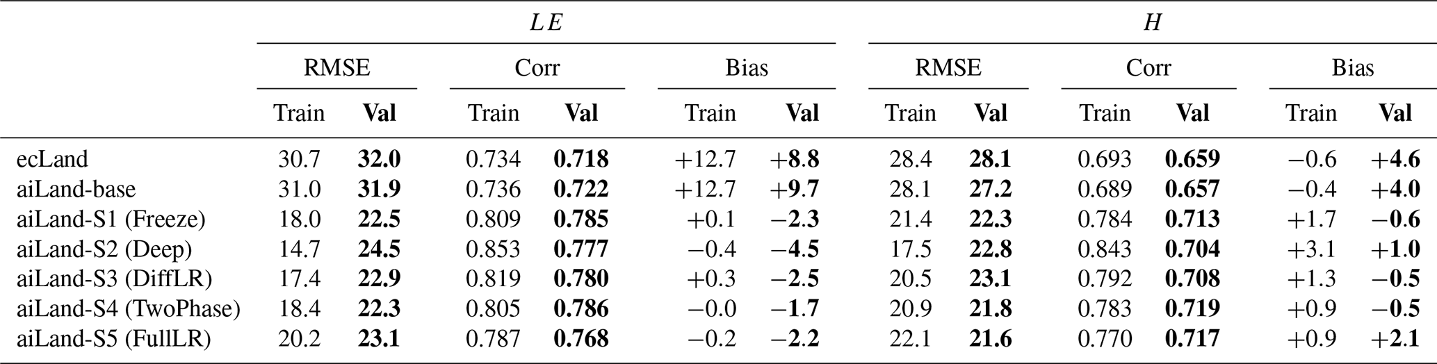
The strategies differ most in how well gains transfer to unseen sites and unseen years. Spatially, the training-validation RMSE gap ranges from 2.9 W m−2 (aiLand-S5) to 9.8 W m−2 (aiLand-S2) for LE, and from −0.5 to 5.3 W m−2 for H. aiLand-S2 achieves the lowest training RMSE but the largest gap, indicating that its randomly initialised diagnostic blocks overfit training-site patterns. aiLand-S4 combines a small spatial gap with the best validation LE correlation (r=0.786, up from 0.722 for aiLand) and validation H correlation (r=0.719, up from 0.657).
Temporal generalisation reinforces this pattern. Comparing validation-site LE improvements between the training period (2000–2019) and the out-of-sample evaluation period (2020–2023), aiLand-S4 is essentially stable (30.2 % vs. 29.6 %) and aiLand-S1 shows only mild attenuation (29.7 % vs. 28.2 %), whereas aiLand-S2 drops markedly (24.2 % vs. 16.5 %). aiLand-S5 is the one case where validation-site improvement strengthens in the evaluation period (27.9 % to 31.9 % for LE; 19.7 % to 15.8 % for H), suggesting that full-model fine-tuning with a low learning rate learns a structural correction rather than memorising site-specific patterns, though at some cost to training-site skill.
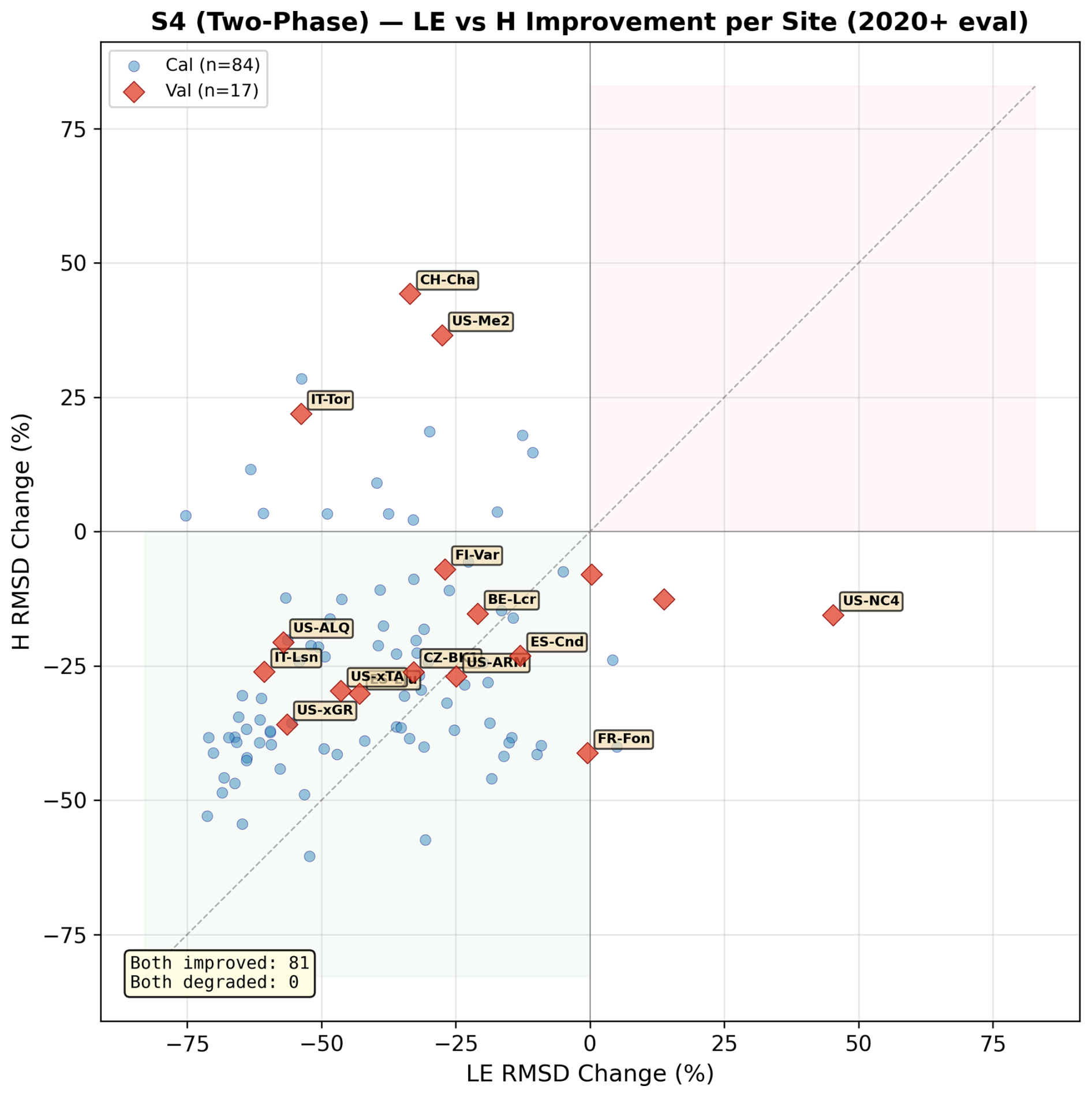
Figure 8Per-site percentage change in RMSE for aiLand-S4 (TwoPhase) relative to aiLand-base during the evaluation period (2020–2023), for LE (x axis) and H (y axis). Each marker represents one FLUXNET site; circles are training sites (n=84) and triangles are validation sites (n=17). Points in the lower-left quadrant indicate improvement in both fluxes simultaneously. Site labels are shown for the largest improvements and degradations.
To illustrate site-level behaviour, we focus on aiLand-S4 as a representative fine-tuning strategy and delivers the best flux RMSE and correlations across validation sites (Table 7). At the site level, aiLand-S4 improves LE at 14 of 17 validation sites and H at 14 of 17; 11 sites improve in both fluxes simultaneously, while no site degrades in both (Fig. 8). The largest LE gains occur at water-limited sites (IT-Lsn, −60.6 %; US-xGR, −56.4 %) and extend across temperate wetland (US-ALQ, −57.2 %) and Mediterranean (IT-Tor, −53.9 %) areas. Three sites show LE degradation: US-NC4 (coastal wetland, +45.2 %), CH-Dav (+13.8 %), and US-xCP (+0.3 %), though all three improve in H. Conversely, three sites with strong LE improvement degrade in H – IT-Tor (+21.9 %), US-Me1 (+36.5 %), and CH-Cha (+44.2 %) – predominantly high-altitude or complex-terrain locations where the ∼60 km grid cannot resolve topographic variability. Figure 9 illustrates these improvements at few validation sites of varying climates and vegetation. We see that ecLand systematically overestimates LE during the growing season. Fine-tuning pulls the model toward the observed flux magnitude while preserving the seasonal phase and inter-annual variability.
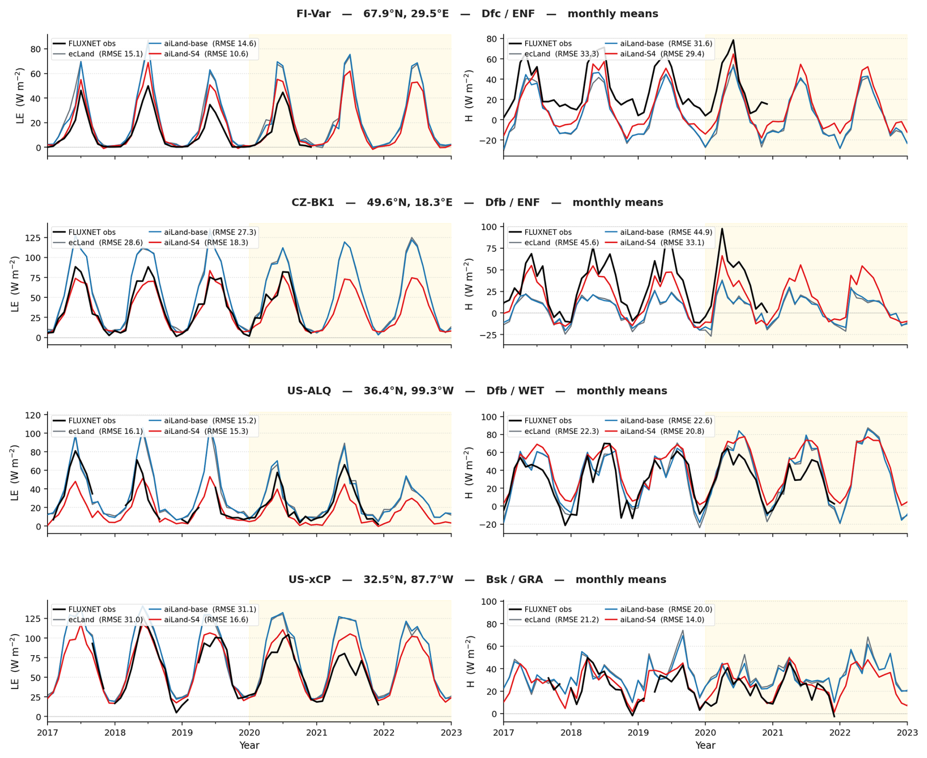
Figure 9LE and H at range of validation sites. Black: FLUXNET observations; grey: ecLand; blue: aiLand-base (pretrained emulator); purple: aiLand-S4 (two-phase fine-tuned). The gold shaded area represents the out-of-sample evaluation period.
3.2.2 Energy partitioning and balance closure
Reductions in LE and H RMSE can, in principle, be achieved either by improving the emulator's energy partitioning or by damping flux magnitudes toward zero. To distinguish these mechanisms, we evaluate two physical-consistency metrics at the FLUXNET sites: the Bowen ratio (), which measures how surface available energy is partitioned between sensible and latent fluxes, and the total turbulent energy balance (H+LE error relative to observations), which tests whether any gains come at the cost of closure. ecLand's median Bowen ratio at validation sites is 0.44 against an observed median of 0.53 (Table 8), reflecting a systematic tendency to partition too much available energy into latent heat relative to sensible heat – consistent with the LE overestimation identified in Sect. 3.2.1 and with analogous biases reported for other LSMs in PLUMBER2 (Abramowitz et al., 2024). All fine-tuned strategies correct this partitioning bias: per-site Bowen ratio MedAE drops from 0.26 (aiLand-base) and 0.22 (ecLand) to between 0.15 and 0.20 across strategies, with aiLand-S4 achieving the lowest value (0.15, a 42 % reduction relative to aiLand-base). Notably, aiLand-S5 recovers the observed median BR exactly but has a higher MedAE (0.20) than aiLand-S4, indicating that a correct bulk ratio does not guarantee correct site-level partitioning. This confirms that the flux RMSE improvements in Sect. 3.2.1 reflect genuine energy-partitioning corrections rather than magnitude damping.
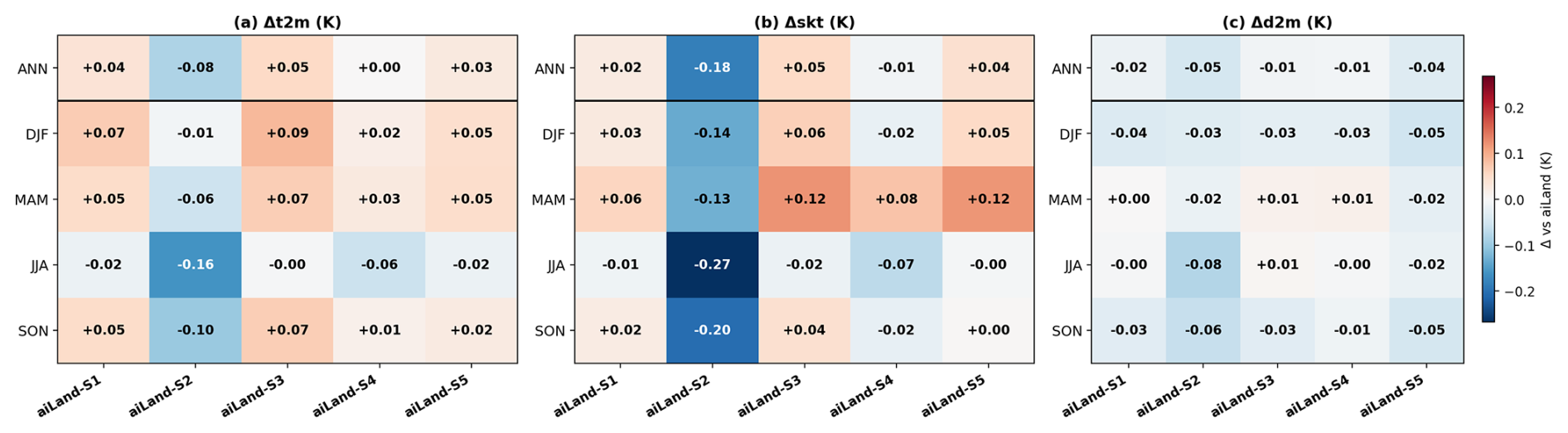
Figure 10Seasonal mean differences (fine-tuned variant–aiLand-base) in screen-level temperature variables across fine-tuning strategies, evaluated at 42 validation sites for 2000–2023. (a) 2 m air temperature, (b) skin temperature, (c) 2 m dew point. Top row of each panel shows annual means; remaining rows show DJF, MAM, JJA, SON. Warm colours indicate model warming relative to aiLand-base; cool colours indicate cooling.
Table 8Energy partitioning and balance closure metrics evaluated over the full observational period (2000–2023) at the 42 validation sites using daily means. BR: Bowen ratio (H LE, computed only when LE>5 W m−2, clipped to [−20, 20]). Median BR: median of per-site median daily BR. BR MedAE: median of per-site median absolute difference between modelled and observed daily BR (median statistics chosen for robustness to the skewed H LE distribution at low LE, where RMSE is dominated by rare outliers). Bias and energy balance residual: mean of per-site time-mean difference (model–obs), reported in W m−2; positive values indicate model overestimation of upward fluxes. All fluxes follow meteorological sign convention (positive upward). Observations (Obs) are from FluxDataKit's energy-balance-closed variant.
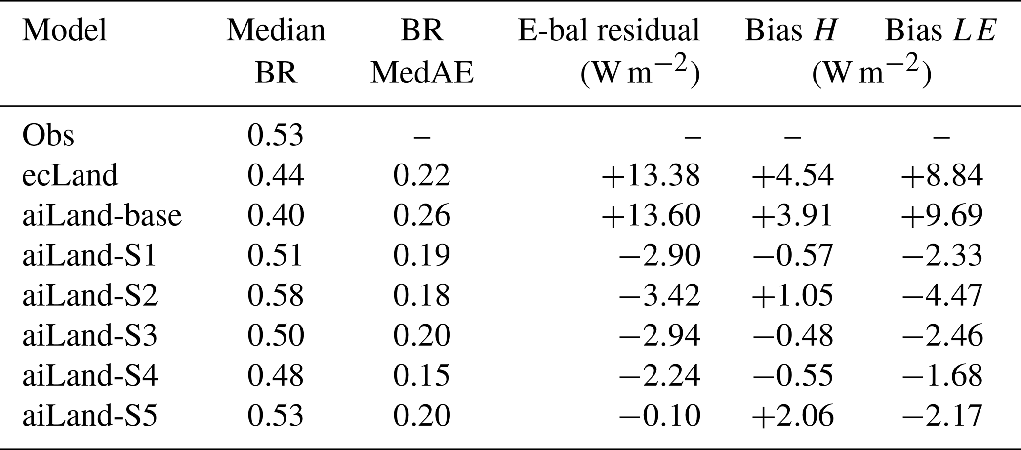
Energy balance closure provides a stricter test. ecLand overestimates both fluxes at validation sites (+8.84 W m−2 for LE, +4.54 W m−2 for H; time-averaged per site), producing a compounding closure offset of +13.38 W m−2. Fine-tuning reverses this bias: all strategies slightly underestimate the turbulent flux sum, with aiLand-S5 achieving near-perfect closure (−0.10 W m−2) and aiLand-S4 second-best (−2.24 W m−2). aiLand-S2 retains the largest offset among fine-tuned models (−3.42 W m−2), consistent with its tendency to overcorrect LE (−4.47 W m−2). Because the observational target used here is an energy-balance-closed flux budget, these results indicate that fine-tuning recovers a physically consistent surface energy balance at the tower scale.
Fine-tuning also produces physically consistent changes in the screen-level diagnostic variables (2 m temperature, 2 m dew point, skin temperature; Fig. 10). Across strategies (excluding aiLand-S2), reduced evaporative cooling at the surface produces a modest warming of skin temperature (+0.02 to +0.05 K) and 2 m temperature (+0.03 to +0.05 K) relative to aiLand-base, while 2 m dew point decreases slightly (−0.01 to −0.04 K), consistent with reduced moisture flux into the boundary layer. aiLand-S4 is notable for near-zero annual temperature change (Δ2t=0.00 K, K), reflecting its more conservative two-phase training schedule. The seasonal partitioning of this response is informative: skin temperature warming peaks in MAM (+0.06 to +0.12 K all strategies excluding aiLand-S2) and remains positive in DJF and SON for most strategies (+0.02 to +0.06 K), but is near-neutral in JJA (−0.02 to −0.00 K, excluding aiLand-S4). aiLand-S4 shows slight cooling in all seasons outside MAM (−0.02 to −0.07 K), reflecting its two-phase schedule. Despite the largest absolute LE correction occurring in summer (∼17 W m−2 in JJA, where aiLand-base overestimates the total upward turbulent flux), fine-tuning corrects this primarily through LE reduction while H changes remain an order of magnitude smaller (<2 W m−2), leaving surface temperature near its baseline value. aiLand-S2 is an exception – its deep diagnostic head produces a cooler skin temperature (−0.18 K annually) and 2 m temperature (−0.08 K) despite similar LE reductions, indicating that an over-parameterised diagnostic-only architecture can decouple the temperature prediction from the surface energy balance.
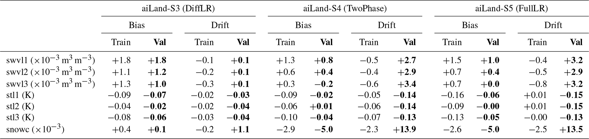
Table 9Prognostic state deviations from aiLand-base during the out-of-sample period 2020–2023. Bias is the time-mean difference (strategy–aiLand-base); Drift is the change over the evaluation window (2023–2020 annual mean). Soil moisture values are given as m3 m−3, soil temperatures in K, and snow cover as fraction, all pre-scaled. These metrics compare model against model (no observations required) therefore computed at all sites with valid predictions: 199 training sites and 42 validation sites.
3.2.3 Prognostic state stability
Strategies aiLand-S1 and aiLand-S2 freeze the prognostic backbone, so their state trajectories are identical to aiLand-base by construction. The backbone-adaptive strategies (aiLand-S3, aiLand-S4, aiLand-S5) modify the backbone and could, in principle, improve flux predictions at the expense of degraded soil moisture or temperature. To assess this, we compare the free-running prognostic trajectories of each fine-tuned model against aiLand-base over the full 24-year period (2000–2023), with focus on the out-of-sample evaluation period (Table 9).
Across the backbone-adaptive strategies, soil moisture is slightly wetter than aiLand-base by 0.3– m3 m−3 and soil temperatures are marginally cooler by 0.02–0.16 K. These offsets are consistent between training and validation sites, indicating a genuine equilibrium shift rather than overfitting. Within-evaluation-period drift is small: soil moisture trends remain below m3 m−3 over four years at training sites, rising to m3 m−3 at validation sites – an order of magnitude smaller than the soil moisture range across regimes, but indicating somewhat more equilibrium shift at unseen locations. Soil temperature trends stay within 0.15 K across both site sets. Snow cover shows a comparable pattern, with validation-site drift of ∼0.014 in fractional cover over four years – small relative to the ∼0.06 snow-cover RMSE already present in the pretrained model (Table 5) and unlikely to materially interact with the snow-coupled error regime identified in Sect. 3.1.2.
The sign of these changes is physically consistent with the flux corrections: the fine-tuned models reduce LE magnitude relative to aiLand-base (correcting a systematic overestimation of evapotranspiration), which is qualitatively consistent with the slight wetting of the soil profile, while the associated reduction in evaporative cooling is consistent with the marginal temperature decrease.
3.2.4 Strategy selection and limitations
Comparing strategies on their combined flux skill and state integrity, aiLand-S3 achieves the smallest prognostic biases and near-zero drift in all variables, while aiLand-S4 and aiLand-S5 show comparable biases but slightly larger variability at validation sites – particularly in soil moisture drift (10−3 m3 m−3 over 4 years) and snow cover. Constraining the backbone learning rate (aiLand-S3) or freezing it entirely (aiLand-S1, aiLand-S2) therefore provides the most robust guard against prognostic instability, while aiLand-S4 and aiLand-S5 trade marginally more state uncertainty for comparable or better flux skill, with downstream effects on screen-level diagnostics consistent with this flux–state tradeoff.
Bringing together the different metrics, aiLand-S4 (two-phase) and aiLand-S5 (full low LR) emerge as the top-performing strategies, with the choice between them depending on application priorities. aiLand-S4 achieves the best flux RMSE, correlations, and per-site Bowen ratio skill (MedAE 0.15) at validation sites, making it preferable when flux prediction accuracy is the primary target. aiLand-S5 achieves near-perfect energy balance closure at validation sites (−0.10 W m−2), recovers the observed median Bowen ratio exactly (0.53), and shows the smallest training–validation generalisation gap, at some cost to training-site flux skill and per-site Bowen ratio accuracy. It is therefore preferable for coupled applications where bulk physical consistency of the surface energy budget matters most. Between the two, aiLand-S5 is also easier to implement since it requires only one phase of fine-tuning.
The same architecture trained from scratch on the fine-tuning dataset improves latent heat flux at the tower sites, but with opposing LE and H biases and a soil-moisture departure from ecLand three to six times that of aiLand-base, suggesting that the prognostic stability of aiLand-base comes from pretraining on the global grid.
Relating these results to the two error sources identified in Sect. 3.1.4: fine-tuning on flux observations reduces the diagnostic-variable errors that underlie the regime sensitivity of latent heat flux, with the largest validation improvements at water-limited sites (IT-Lsn −60.6 %, US-xGR −56.4 %) and consistent gains at boreal, temperate and Mediterranean sites. Snow-coupled errors are not addressed by diagnostic-head fine-tuning, as both originate in the prognostic increment function. Correcting these prognostic-level errors would require updating the state-evolution network itself, for example through fine-tuning on snow-specific observational data or online bias correction, which we leave to future work.
A consideration in interpreting these results is the scale mismatch between FLUXNET tower footprints (∼100 m) and the N320 reduced Gaussian grid (∼31 km at the equator, ∼60 km at mid-latitudes). The model represents grid-cell-averaged fluxes, whereas tower observations capture local conditions that may not be representative of the surrounding landscape – particularly at sites with heterogeneous land cover, complex terrain, or coastal boundaries. This mismatch contributes to irreducible representation error in the metrics and likely explains some of the site-level degradations observed at high-altitude (CH-Cha, US-Me1) and coastal (US-NC4) locations, where sub-grid variability is largest.
Similarly, while we use energy-balance-closed FLUXNET observations, some caveats remain. The closure correction distributes the residual energy proportionally between H and LE, preserving the observed Bowen ratio but making absolute flux magnitudes conditional on this convention rather than uniquely determined. Net radiation and ground heat flux measurements used in the correction have their own ∼10 %–15 % uncertainty (Mauder et al., 2020), which propagates into the closed fluxes. Bowen ratio as a metric is also disproportionately sensitive to low-LE conditions where the ratio diverges.
Read together, the cross-regime and fine-tuning experiments make a case for physical pretraining that goes beyond the emulation of one model: the mapping learned from ecLand transfers across regimes and survives the removal of a regime from training (Table 6). In addition, it is retained rather than overwritten when adjusted towards sparse observations. Transferable physical structure plus observational correction is what an ML land surface component would require where the observational record is sparse
4.1 Towards a data-driven Earth System Model
This work is part of the broader Destination Earth effort to develop a fully data-driven Earth System Model (see https://destine.ecmwf.int/ml-earth-system-components/, last access: 10 November 2026). It is also embedded within the Copernicus Climate Change Service Evolution (CERISE) project, which aims to develop next-generation climate and land reanalyses – a context in which fast, differentiable land surface emulators offer particular value. In its current configuration, aiLand emulates a core set of land surface variables from ecLand, including soil moisture, soil temperature, snow cover, latent and sensible heat fluxes, skin temperature, as well as near-surface atmospheric diagnostics such as 2 m temperature and 2 m dew point. These variables represent key components of the land–atmosphere exchange of water and energy and constitute a first step towards a data-driven representation of land surface processes suitable for coupling within an Earth system context.
A natural next extension is the inclusion of runoff and related hydrological fluxes. Runoff provides the primary interface between the land surface and hydrological routing and streamflow models, and its accurate representation is essential for coupling land surface processes to river discharge, flood forecasting, and freshwater budgets. Emulating runoff alongside soil and snow states would enable aiLand to interact more directly with streamflow and routing models, supporting experiments on land–hydrology coupling and the propagation of land surface uncertainties into river discharge.
Beyond runoff, future developments may extend emulation to a broader range of land surface variables, including both observed quantities such as leaf area index (LAI) and vegetation phenology, and internal model states that are not directly observable but are critical for coupling with other Earth system components. Near-surface wind, which ecLand diagnoses but which in offline mode is largely determined by the atmospheric forcing, would become a relevant diagnostic target in coupled configurations, where the land surface influences it through roughness and momentum exchange. Expanding the set of emulated variables would strengthen the role of aiLand as an intermediate layer between observations and the physical land surface model, enabling richer diagnostics, calibration, and process-level evaluation. In parallel, observational products for variables already emulated, such as satellite-derived soil moisture and land surface temperature, could be used to fine-tune the corresponding prognostic and diagnostic outputs, in the same way as FLUXNET fluxes are used here.
More generally, a central open question concerns how ML-based land surface emulators, such as the aiLand model explored here, should be coupled with other Earth system components, including the atmosphere (Lang et al., 2024), ocean (Hahner et al., 2026), and hydrological routing and streamflow models (Taccari et al., 2026), to create a full data-driven Earth System Model. Ensuring stability and physical consistency across component interfaces remains an active area of research. Notably, several land variables, including soil moisture, soil temperature, runoff, and snow, are already successfully integrated within ECMWF’s Artificial Intelligence Forecasting System (AIFS, Moldovan et al., 2026; Raoult et al., 2025b). In that system, these variables are learned jointly within a single end-to-end ML framework, allowing cross-variable dependencies and feedbacks to be captured implicitly during training rather than imposed through a posteriori coupling. aiLand's differentiability also makes it a candidate for hybrid configurations, where it could replace selected ecLand parameterisations while the surrounding physics enforces conservation. Looking forward, ongoing work is migrating aiLand training fully into the anemoi framework – the same stack used for the AIFS – providing a shared codebase that improves traceability and maintenance, and structurally simplifies future coupling experiments across ECMWF's ML-based Earth system components.
4.2 Data assimilation and parameter estimation
Machine-learning emulators of land surface models offer new perspectives for data assimilation (DA) and parameter estimation, particularly when trained to reproduce an existing physical scheme. In this study, aiLand is trained to emulate ECMWF's land surface model ecLand, ensuring that the learned relationships remain physically informed by process-consistent simulations. Fine-tuning is demonstrated using FLUXNET eddy-covariance observations as an illustrative example, rather than as a comprehensive observational assimilation. The methodology, however, is fully extensible and could incorporate a wider range of observational datasets – from in situ networks to satellite derived products – in future studies.
A first and immediate application of such emulators is rapid offline experimentation. Parameter estimation and sensitivity analysis in land surface models are computationally expensive, particularly in ensemble-based DA settings and high-dimensional parameter spaces (Raoult et al., 2025a). aiLand evaluations are orders of magnitude faster than ecLand, enabling systematic offline testing of parameter sensitivities, regime-dependent behaviour, and observation–model mismatches. This allows efficient narrowing of parameter spaces and targeted exploration of model deficiencies.
The differentiability of MLP-based emulators further enables gradient-based parameter optimisation and observation-constrained learning without requiring explicit tangent-linear or adjoint formulations of ecLand. Fine-tuning aiLand against FLUXNET surface fluxes demonstrates how observational constraints can be incorporated efficiently while retaining the dynamics learned from ecLand simulations. From a DA perspective, this serves as an offline analogue to variational calibration, providing insights into parameter sensitivities under observational constraints without directly modifying operational DA systems.
The complementary case of gradient-based parameter optimisation has clearer limits in the current configuration. Although several physically meaningful parameters enter the emulator through static physiographic input fields – including soil hydraulic properties such as permanent wilting point and field capacity, which vary spatially across soil texture classes – the broader set of tunable ecLand process parameters (e.g., skin thermal conductivities, stomatal resistance and conductance) is not exposed as input controls. Preliminary experiments have shown that perturbing the existing static input fields produces physically consistent responses in prognostic states such as soil moisture, suggesting a pathway toward parameter sensitivity analysis within the emulator framework. The model has so far only seen these parameters in their natural co-variation with other inputs (vegetation type, climate, soil descriptors), so robust isolated parameter perturbation experiments would require additional targeted ecLand simulations spanning the parameter space independently of the other input variables. Future developments could therefore extend the input set to include further ecLand process parameters as controlled input dimensions, enabling gradient-based calibration and sensitivity analysis of land-surface characteristics while retaining the computational efficiency of the emulator.
In addition, such emulators can reduce computational cost in coupled or weakly coupled land–atmosphere DA (de Rosnay et al., 2022). In ensemble-based systems, repeated evaluation of the land surface model across ensemble members contributes substantially to computational demand (Fairbairn et al., 2019). Fast emulators could act as surrogate forward models in selected components of the DA workflow – for example, for ensemble generation, sensitivity experiments, or observation operators – potentially enabling larger ensembles or more frequent cycling at lower computational cost. Operational integration of ML surrogates into DA systems will require systematic investigation of stability, error propagation, and controllability, which is outside the scope of the present study.
Beyond DA itself, fast and differentiable land surface emulators are also relevant to the production of high-resolution, multi-decadal land reanalyses. The computational cost of multi-decadal ecLand integrations limits how finely current and future land reanalyses can be resolved, and the stability of aiLand over multi-year forced integrations (Sect. 3.1.1) suggests it could enable higher-resolution or larger-ensemble reanalysis production – particularly relevant for Copernicus Climate Change Service users within the broader CERISE objectives.
Finally, aiLand provides a diagnostic framework for physical model development. Systematic corrections learned during fine-tuning against FLUXNET fluxes can reveal compensating errors, missing processes, or regime-dependent biases in ecLand, guiding targeted improvements to parameterisations. In this sense, ML acts as a complementary tool to traditional process-based evaluation, rather than a replacement for the physical model (Abramowitz et al., 2024; Reichstein et al., 2019) ensuring physical consistency, rather than data-driven correlations between states. Future work could expand the observational base, allowing broader evaluation and calibration across climates, land covers, and surface processes. Within this broader perspective, physically informed ML emulators such as aiLand offer a practical pathway to accelerate model development while preserving consistency with established land surface physics.
4.3 Architecture and physical constraints
The applications above also bear on how the architecture itself should develop. The multi-layer perceptron used here operates point-wise and represents neither spatial context nor memory beyond the previous state. The absence of spatial context mirrors the structure of the target: ecLand solves each grid box as an independent column, with no lateral exchange within the land scheme, so a point-wise emulator matches the physical model rather than approximating a spatial one. In coupled mode, neighbouring columns interact only through the atmosphere. Because the model never sees the grid it is also largely resolution-agnostic (Appendix C), whereas transformer or graph-based architectures over the model grid would add representational capacity that the target does not use and would tie the learned representation to a particular discretisation. This argument is bounded by resolution and by scope: lateral transport becomes increasingly relevant as grid spacing decreases, and the runoff and routing extension of Sect. 4.1 is where the land surface stops being column-independent, so an emulator coupled to a routing model would need to represent connectivity between grid boxes. Temporal context involves a different trade-off, since recurrence adds internal state that must be carried through the rollout. Wesselkamp et al. (2025) found a tuned LSTM advantageous for snow and upper-layer soil temperature over Europe, but this did not carry over to the global scale, where the MLP performed best of the three architectures tested and is the only one that is both differentiable and inexpensive to evaluate, as the applications in Sect. 4.2 require.
A second question is whether the emulator conserves energy and water. aiLand does not enforce conservation through loss penalties or architectural constraints, but neither is it unconstrained: it is trained on a model whose surface budgets close by construction, so approximate conservation is inherited as a learned property of the mapping. The results suggest this inheritance is substantial; the state remains coherent over four-year integrations (Sect. 3.1.1), and the fine-tuned variants improve energy balance closure although no closure term appears in the loss (Sect. 3.2.2). What learned consistency cannot offer is a guarantee, and it is most likely to fail in rare states, unseen regimes and long coupled integrations, where conservation matters most. Making the constraint explicit is not straightforward: the observational fine-tuning target is an energy-balance-closed product in which the residual is distributed by convention rather than measured (Sect. 2.1.4), so a model constrained to satisfy that closure would inherit the convention as a structural commitment. Whether hard constraints or soft penalties are preferable depends on the application, and we regard this as an open question for emulators of this kind.
We have presented aiLand, a stand-alone MLP-based, limited processes, emulator of ECMWF's ecLand land surface scheme, trained in a two-stage framework that combines pretraining on ecLand outputs with fine-tuning on FLUXNET eddy-covariance observations. The pretrained emulator reproduces ecLand's prognostic and diagnostic states with high skill at short lead times, remains stable over continuous 4-year autoregressive integrations, with a small intrinsic warm bias (+0.40 K in stl1) arising from the interaction between the Smooth L1 loss and the right-skewed soil-temperature increment distribution. The emulator generalises cleanly across ecosystem regimes: a single globally trained model matches regime-specialist performance in-regime, outperforms specialist transfers for the temperate and rainforest regimes, and loses at most 16 % of its skill on a regime withheld entirely from training. Complementary experiments indicate that the residual architecture also transfers between spatial resolutions (Appendix B). Residual errors concentrate in snow-insulated cold regimes, where the insulating snowpack decouples the soil column from atmospheric forcing, and in extreme aridity regimes where the surface energy balance differs sharply from vegetated training environments. Both error regimes correspond to long-standing limitations of ecLand and land surface models more broadly – cold-region snow and freeze-thaw representation, and arid-region surface flux sensitivity to soil moisture thresholds – so the spatial and regime-dependent error patterns exposed by these robustness tests provide a structured diagnostic of where ecLand's input–output relationships are hardest to learn, supporting the use of the emulator not only as a surrogate but as an interpretive tool for prioritising physical model development.
Fine-tuning on flux observations reduces validation-site latent heat flux RMSE by 30 % and sensible heat flux by 20 % while preserving prognostic state integrity, and simultaneously recovers a physically consistent surface energy budget at the tower scale:per-site Bowen ratio error drops by 42 % (MedAE; best in aiLand-S4) and the energy balance closure residual is reduced from +13.4 W m−2 (pretrained) to within 0.1 W m−2 at validation sites (aiLand-S5). The snow-coupled errors identified in the pretrained model are not addressed by this form of fine-tuning, as they originate in the prognostic increment function rather than the diagnostic mapping; correcting them will require observational constraints on the state evolution itself.
Several broader limitations apply to this work. Fine-tuning on a single observational network does not guarantee robustness across regions or climates, and there is a risk that learned corrections compensate for structural model errors rather than resolving them. Relatedly, both pretraining and fine-tuning here sample predominantly typical conditions, so the emulator's behaviour under rare or unprecedented extremes – precisely the regime where purely data-driven systems are most prone to extrapolation failure (Zhang et al., 2026; Cranko Page et al., 2026) – remains largely untested. Deliberately enriching the training distribution with extreme events, or up-weighting them in the loss, is therefore a promising direction for improving robustness in exactly the conditions of greatest societal relevance. The effectiveness of both training and evaluation depends critically on the availability of high-quality, long-term observational records: sustained investment in in situ measurement networks and satellite missions is therefore essential to ensure that the capacity to constrain, validate, and improve both physical models and their ML surrogates is not fundamentally limited. These results should be interpreted as a proof of concept, illustrating how physically informed ML emulators can support offline experimentation, methodological development, and preparatory work for broader data assimilation applications.
Future work will extend fine-tuning to additional observational streams – including satellite-derived soil moisture, surface temperature, and vegetation dynamics observables such as solar-induced fluorescence – explore coupling to the atmospheric component of the IFS, and exploit aiLand's differentiability for gradient-based land surface parameter estimation and data assimilation.
To relate the climate–land-surface regimes of Sect. 2.3.2 to an established classification, each land grid point was assigned to an aggregated Köppen–Geiger group and the two partitions were cross-tabulated (Table A1). The regimes are, to good approximation, an aggregated Köppen classification: R5 and R4 are the rainforest and desert cores, R2 and R3 the warm and cold sides of the continental group, and R1 the steppe margin.
The clustering departs from Köppen in two ways. It adds two splits that Köppen does not make at group level: the tropical group is divided between a rainforest core (R5, 40 % of tropical cells) and a seasonal humid cluster (R0, 50 %), and the arid group between desert (R4) and steppe (R1). It also dissolves two distinctions that are redundant for the prognostic soil state: 66 %–79 % of the temperate C classes (oceanic, Mediterranean, monsoon) are absorbed into R0, which therefore extends into maritime Europe, and 72 % of the polar E class is absorbed into the boreal regime R3.
Table A1Composition of each regime by aggregated Köppen–Geiger group, as a percentage of the regime's grid cells (row-normalised). Groups contributing less than 6 % of a regime are omitted, so rows do not sum to 100 %.
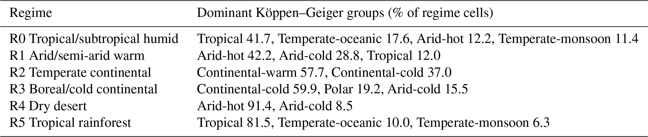
The FluxDataKit (Hufkens and Stocker, 2025) provides eddy-covariance observations from 339 FLUXNET sites worldwide (Pastorello et al., 2020). We apply a two-stage filtering process. First, quality-control filtering removes 93 sites with excessive stuck-sensor values or insufficient valid latent and sensible heat flux observations, leaving 246 sites. Second, because multiple FLUXNET sites can fall within a single grid cell of the N320 reduced Gaussian grid, we retain only one representative site per grid cell 00 the site with the highest data-quality score – removing a further 5 co-located sites and leaving 241 sites in total. The sites are split into 199 training sites used for fine-tuning and 42 independent validation sites held out for evaluation. The split is stratified by IGBP vegetation type so that the relative proportion of each land-cover class is preserved in both subsets (approximately 82 %/18 % training/validation), ensuring that the validation set is representative of the same vegetation and climate diversity as the training set (Fig.B1). Of the 42 validation sites, 17 have flux observations in the post-2020 hold-out period (Table B1), enabling a fully out-of-sample temporal evaluation.
Table B1Validation sites with flux observations in the 2020+ hold-out period (17 of 42 held-out sites). Vegetation type follows the IGBP land-use classification; climate zone follows the Köppen–Geiger scheme.
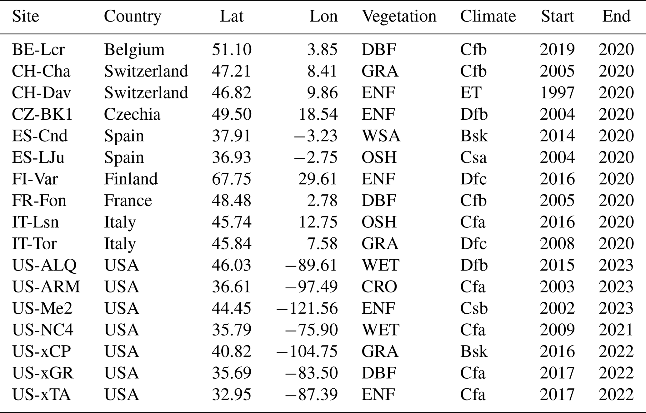
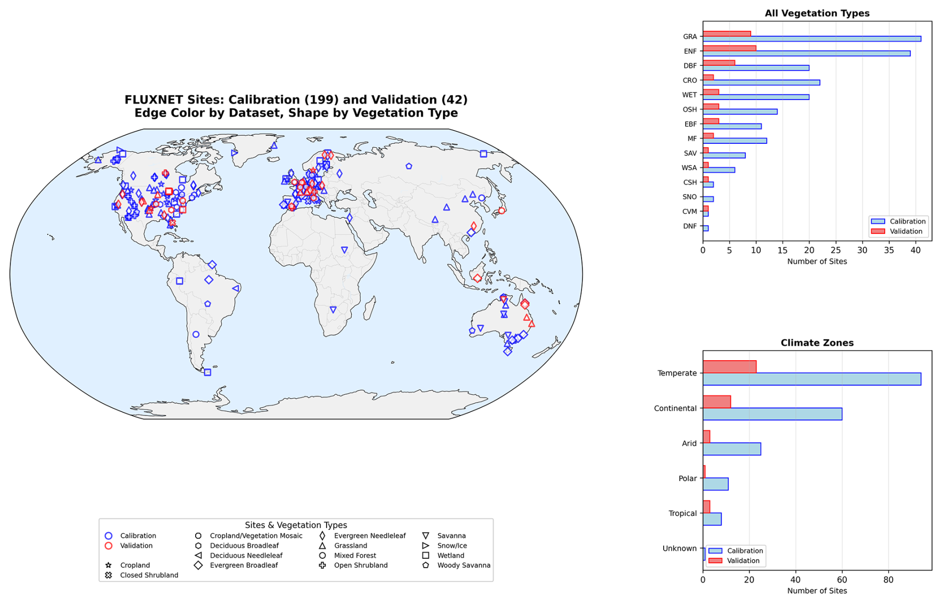
Figure B1Geographic distribution of the 241 FLUXNET sites used in this study, split into 199 training (blue) and 42 validation (red) sites. Marker shapes denote IGBP vegetation type. The split is stratified by vegetation class so that both subsets span the same range of land-cover and climate conditions. Right panels show the distribution of vegetation types (top panel) and Köppen–Geiger climate zones (bottom panel) for each subset. FLUXNET data courtesy of the FLUXNET network (Pastorello et al., 2020).
The cross-regime experiments in Sect. 3.1.3 showed that prognostic state predictions transfer cleanly across ecosystem regimes while diagnostic outputs are more sensitive to the training distribution. A complementary question is whether the same asymmetry holds across spatial resolutions: does a model trained on one grid generalise to another, and does the prognostic–diagnostic split persist? To answer this, we trained an additional aiLand instance on an O96 ecLand simulation (∼125 km resolution), using the same setup as the N320 model. Each model was evaluated on its native grid and on the alternative resolution (Table C1).
For same-resolution evaluation, the two models achieve comparable prognostic RMSE. O96 is marginally better for deep soil layers (stl3: 0.068 K for O96 vs. 0.078 K for N320) and snow cover, while N320 is better for near-surface diagnostics (2 m temperature: 0.616 K for N320 vs. 0.876 K for O96) and surface fluxes (sensible heat: 11.01 W m−2 for N320 vs. 11.57 W m−2 for O96), likely reflecting the richer spatial heterogeneity captured at higher resolution.
Cross-resolution transfer is asymmetric. The O96 model transfers to N320 with modest prognostic degradation (mean ratio 1.057) and near-neutral diagnostic performance (mean ratio 1.018). The N320 model evaluated on O96 shows improved prognostic skill (mean ratio 0.959) but substantially degraded diagnostics (mean ratio 1.289), particularly for 2 m temperature (ratio 1.737). The N320 model, having learned fine-scale surface–atmosphere coupling, struggles to reproduce the smoother diagnostic fields of the coarser grid, while its prognostic predictions – which depend mainly on local forcing and static descriptors 00 generalise well or even improve. The N320 grid sits near the threshold at which some mesoscale processes (e.g. organised convection, mountain–valley flows) are partially resolved in ERA5 forcing, whereas at O96 these are firmly subgrid; the asymmetric diagnostic degradation may therefore reflect, in part, the loss of mesoscale variability that the high-resolution model has implicitly used as a predictor.
These results confirm that the point-wise MLP architecture is largely resolution-agnostic for prognostic states. Diagnostic outputs – especially 2 m temperature and surface fluxes – remain sensitive to the spatial characteristics of the training grid, consistent with the diagnostic sensitivity observed in the cross-regime analysis. For operational applications, a model trained at one resolution can therefore provide reliable state predictions at alternative grids, though diagnostic outputs may benefit from resolution-specific training. RMSE values reported correspond to single-timestep predictions; autoregressive rollouts up to 10 d (40 steps) show negligible additional error accumulation, with cross-resolution transfer ratios remaining stable across all lead times.
Table C1Prognostic and diagnostic RMSE for models trained at O96 and N320 resolutions for single-timestep predictions. Each cell reports either the same-resolution RMSE (shaded) or the RMSE for the alternative resolution together with the ratio relative to the corresponding same-resolution RMSE. Mean and median ratios summarise cross-resolution changes. Surface heat fluxes (H, LE) are reported in W m−2 as time-averaged power over each 6-hourly timestep.
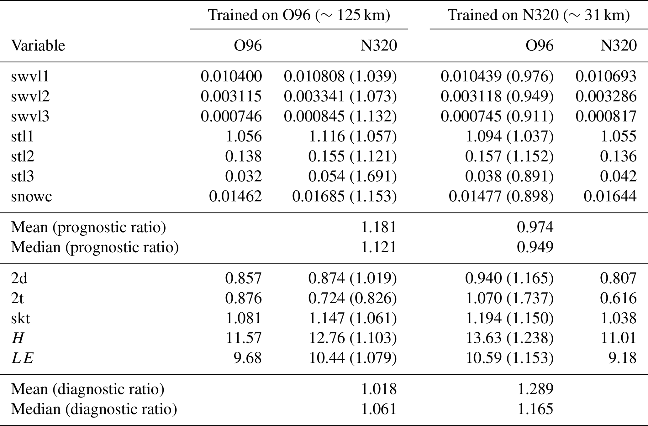
Code for training, inference, and analysis, together with the aiLand-base checkpoint, can be found at https://doi.org/10.5281/zenodo.20764680 (Raoult and Pinnington, 2026). Training data are published at https://doi.org/10.21957/0f6t-7f73 (n320; Raoult et al., 2026a) and https://doi.org/10.21957/fs25-c406 (o96; Raoult et al., 2026b). These datasets are ecLand offline runs, generated using ecLand (Nawab et al., 2025, https://doi.org/10.5281/zenodo.21995581) forced by ERA5 (Hersbach et al., 2020), which is distributed through the Copernicus Climate Data Store (https://cds.climate.copernicus.eu, last access: 10 November 2026). FLUXNET observations were obtained from the FluxDataKit harmonised dataset (Hufkens and Stocker, 2025, https://doi.org/10.5281/zenodo.14808331), which compiles openly available eddy-covariance data from the FLUXNET2015 (Pastorello et al., 2020), PLUMBER2 (Abramowitz et al., 2024), AmeriFlux (Novick et al., 2018), and ICOS (https://doi.org/10.18160/2G60-ZHAK, Warm Winter 2020 Team and ICOS Ecosystem Thematic Centre, 2022) networks.
NR and EP conceptualised the study. EP built the first prototype of aiLand, NR extended the framework to interface with anemoi and the ability to fine-tune against observations. NR ran the analysis and generated the figures, with strong support from EP. MSC provided technical support on the anemoi, and FP, BR and NZ on specifically on anemoi-datasets. GA, GB and SB are key developers of ecLand and provided knowledge on the physical model. PdR and CR provided further expertise on the physical modelling side, and MC and PD on the ML side. All authors contributed to the writing of the manuscript.
The contact author has declared that none of the authors has any competing interests.
Views and opinions expressed are however those of the authors only and do not necessarily reflect those of the European Union or the Commission. Neither the European Union nor the granting authority can be held responsible for them.
Publisher's note: Copernicus Publications remains neutral with regard to jurisdictional claims made in the text, published maps, institutional affiliations, or any other geographical representation in this paper. The authors bear the ultimate responsibility for providing appropriate place names. Views expressed in the text are those of the authors and do not necessarily reflect the views of the publisher.
This work was supported by Destination Earth Phase 2, under which prototypes for multiple Earth system components have been developed. Destination Earth is a European Union – funded initiative launched in 2022 to build a digital replica of the Earth system by 2030. It is jointly implemented by the European Centre for Medium-Range Weather Forecasts (ECMWF), the European Space Agency (ESA), and the European Organisation for the Exploitation of Meteorological Satellites (EUMETSAT).
We further would like to thank colleagues at ECMWF and across Member States for their continued development of the Anemoi framework and the IFS model. We also would like to thank colleagues at ECMWF working on machine-learning Earth system components within Destination Earth for technical advice and support. We also acknowledge the Code4Earth ML-BEES project (https://github.com/ECMWFCode4Earth/ML-BEES, last access: 10 November 2026) for validating the initial prototype, and thank Christoph Herbert and Peter Weston for their supervision during the Code4Earth project. Finally, we would like to thank the two anonymous reviewers for their constructive feedback, which greatly helped to improve the quality of this manuscript.
This research has been supported by the European Union's Digital Europe Programme through Destination Earth (DestinE), and by the European Union's Horizon Europe research and innovation programme through CERISE (Copernicus Climate Change Service Evolution; grant no. 101082139).
This paper was edited by Donghui Xu and reviewed by three anonymous referees.
Abramowitz, G., Ukkola, A., Hobeichi, S., Cranko Page, J., Lipson, M., De Kauwe, M. G., Green, S., Brenner, C., Frame, J., Nearing, G., Clark, M., Best, M., Anthoni, P., Arduini, G., Boussetta, S., Caldararu, S., Cho, K., Cuntz, M., Fairbairn, D., Ferguson, C. R., Kim, H., Kim, Y., Knauer, J., Lawrence, D., Luo, X., Malyshev, S., Nitta, T., Ogee, J., Oleson, K., Ottlé, C., Peylin, P., de Rosnay, P., Rumbold, H., Su, B., Vuichard, N., Walker, A. P., Wang-Faivre, X., Wang, Y., and Zeng, Y.: On the predictability of turbulent fluxes from land: PLUMBER2 MIP experimental description and preliminary results, Biogeosciences, 21, 5517–5538, https://doi.org/10.5194/bg-21-5517-2024, 2024. a, b, c, d, e, f
Ba, J. L., Kiros, J. R., and Hinton, G. E.: Layer Normalization, arXiv [preprint], arXiv:1607.06450, https://doi.org/10.48550/arXiv.1607.06450, 2016. a
Baldocchi, D., Falge, E., Gu, L., Olson, R., Hollinger, D., Running, S., Anthoni, P., Bernhofer, C., Davis, K., Evans, R., Fuentes, J., Goldstein, A., Katul, G., Law, B., Lee, X., Malhi, Y., Meyers, T., Munger, W., Oechel, W., Paw U, K. T., Pilegaard, K., Schmid, H. P., Valentini, R., Verma, S., Vesala, T., Wilson, K., and Wofsy, S.: FLUXNET: A new tool to study the temporal and spatial variability of ecosystem-scale carbon dioxide, water vapor, and energy flux densities, B. Am. Meteorol. Soc., 82, 2415–2434, 2001. a
Balsamo, G., Beljaars, A., Scipal, K., Viterbo, P., van den Hurk, B., Hirschi, M., and Betts, A. K.: A revised hydrology for the ECMWF model: Verification from field site to terrestrial water storage and impact in the Integrated Forecast System, J. Hydrometeorol., 10, 623–643, 2009. a
Bao, S., Alonso, L., Wang, S., Gensheimer, J., De, R., and Carvalhais, N.: Toward robust parameterizations in ecosystem-level photosynthesis models, J. Adv. Model. Earth Syst., 15, e2022MS003464, https://doi.org/10.1029/2022MS003464, 2023. a
Bao, S., Carvalhais, N., Xu, J., Chen, J. M., Lei, Y., Tana, G., Lin, C., and Shi, J.: Global distribution pattern in characteristics of gross primary productivity response to soil water availability, Agr. Forest Meteorol., 372, 110701, https://doi.org/10.1016/j.agrformet.2025.110701, 2025. a
Blyth, E. M., Arora, V. K., Clark, D. B., Dadson, S. J., De Kauwe, M. G., Lawrence, D. M., Melton, J. R., Pongratz, J., Turton, R. H., Yoshimura, K., and Yuan, H.: Advances in land surface modelling, Curr. Clim. Change Rep., 7, 45–71, 2021. a
Boussetta, S., Balsamo, G., Beljaars, A., Agustí-Panareda, A., Calvet, J.-C., Jacobs, C., van den Hurk, B., Viterbo, P., Lafont, S., Dutra, E., Jarlan, L., Balzarolo, M., Papale, D., and van der Werf, G.: Natural land carbon dioxide exchanges in the ECMWF integrated forecasting system: Implementation and offline validation, J. Geophys. Res.-Atmos., 118, 5923–5946, 2013. a
Boussetta, S., Balsamo, G., Arduini, G., Dutra, E., McNorton, J., Choulga, M., Agustí-Panareda, A., Beljaars, A., Wedi, N., Muñoz-Sabater, J., de Rosnay, P., Sandu, I., Hadade, I., Carver, G., Mazzetti, C., Prudhomme, C., Yamazaki, D., and Zsoter, E.: ECLand: The ECMWF land surface modelling system, Atmosphere, 12, 723, https://doi.org/10.3390/atmos12060723, 2021. a, b, c, d
Bush, M., Flack, D. L. A., Lewis, H. W., Bohnenstengel, S. I., Short, C. J., Franklin, C., Lock, A. P., Best, M., Field, P., McCabe, A., Van Weverberg, K., Berthou, S., Boutle, I., Brooke, J. K., Cole, S., Cooper, S., Dow, G., Edwards, J., Finnenkoetter, A., Furtado, K., Halladay, K., Hanley, K., Hendry, M. A., Hill, A., Jayakumar, A., Jones, R. W., Lean, H., Lee, J. C. K., Malcolm, A., Mittermaier, M., Mohandas, S., Moore, S., Morcrette, C., North, R., Porson, A., Rennie, S., Roberts, N., Roux, B., Sanchez, C., Su, C.-H., Tucker, S., Vosper, S., Walters, D., Warner, J., Webster, S., Weeks, M., Wilkinson, J., Whitall, M., Williams, K. D., and Zhang, H.: The third Met Office Unified Model–JULES Regional Atmosphere and Land Configuration, RAL3, Geosci. Model Dev., 18, 3819–3855, https://doi.org/10.5194/gmd-18-3819-2025, 2025. a
Caliński, T. and Harabasz, J.: A dendrite method for cluster analysis, Commun. Stat., 3, 1–27, https://doi.org/10.1080/03610927408827101, 1974. a
Chaney, N. W., Van Huijgevoort, M. H. J., Shevliakova, E., Malyshev, S., Milly, P. C. D., Gauthier, P. P. G., and Sulman, B. N.: Harnessing big data to rethink land heterogeneity in Earth system models, Hydrol. Earth Syst. Sci., 22, 3311–3330, https://doi.org/10.5194/hess-22-3311-2018, 2018. a
Chen, T., He, T., Benesty, M., Khotilovich, V., Tang, Y., Cho, H., Chen, K., Mitchell, R., Cano, I., Zhou, T., Li, M., Xie, J., Lin, M., Geng, Y., Li, Y., Yuan, J., and Cortes, D.: Xgboost: extreme gradient boosting, R package version 0.4-2, The R Foundation, 1–4, https://doi.org/10.32614/cran.package.xgboost, 2015. a
Cheruy, F., Ducharne, A., Hourdin, F., Musat, I., Vignon, É., Gastineau, G., Bastrikov, V., Vuichard, N., Diallo, B., Dufresne, J.-L., Ghattas, J., Grandpeix, J.-Y., Idelkadi, A., Mellul, L., Maignan, F., Ménégoz, M., Ottlé, C., Peylin, P., Servonnat, J., Wang, F., and Zhao, Y.: Improved near-surface continental climate in IPSL-CM6A-LR by combined evolutions of atmospheric and land surface physics, J. Adv. Model. Earth Syst., 12, e2019MS002005, https://doi.org/10.1029/2019MS002005, 2020. a
Choulga, M., Kourzeneva, E., Balsamo, G., Boussetta, S., and Wedi, N.: Upgraded global mapping information for earth system modelling: an application to surface water depth at the ECMWF, Hydrol. Earth Syst. Sci., 23, 4051–4076, https://doi.org/10.5194/hess-23-4051-2019, 2019. a
Clark, M. P., Nijssen, B., Lundquist, J. D., Kavetski, D., Rupp, D. E., Woods, R. A., Freer, J. E., Gutmann, E. D., Wood, A. W., Brekke, L. D., Arnold, J. R., Gochis, D. J., and Rasmussen, R. M.: A unified approach for process-based hydrologic modeling: 1. Modeling concept, Water Resour. Res., 51, 2498–2514, 2015. a
Cranko Page, J., De Kauwe, M. G., Pitman, A. J., Towers, I. R., Arduini, G., Best, M. J., Ferguson, C. R., Knauer, J., Kim, H., Lawrence, D. M., Nitta, T., Oleson, K. W., Ottlé, C., Ukkola, A., Vuichard, N., Wang-Faivre, X., and Abramowitz, G.: Land surface model underperformance tied to specific meteorological conditions, Biogeosciences, 23, 263–282, https://doi.org/10.5194/bg-23-263-2026, 2026. a, b
Dagon, K., Sanderson, B. M., Fisher, R. A., and Lawrence, D. M.: A machine learning approach to emulation and biophysical parameter estimation with the Community Land Model, version 5, Adv. Stat. Clim. Meteorol. Oceanogr., 6, 223–244, 2020. a
Davies, D. L. and Bouldin, D. W.: A cluster separation measure, IEEE T. Pattern Anal. Mach. Intel., PAMI-1, 224–227, https://doi.org/10.1109/TPAMI.1979.4766909, 1979. a
de Rosnay, P., Browne, P., de Boisséson, E., Fairbairn, D., Hirahara, Y., Ochi, K., Schepers, D., Weston, P., Zuo, H., Alonso-Balmaseda, M., Balsamo, G., Bonavita, M., Bormann, N., Brown, A., Chrust, M., Dahoui, M., De Chiara, G., English, S., Geer, A., Healy, S., Hersbach, H., Laloyaux, P., Magnusson, L., Massart, S., McNally, A., Pappenberger, F., and Rabier, F.: Coupled data assimilation at ECMWF: current status, challenges and future developments, Q. J. Roy. Meteorol. Soc., 148, 2672–2702, 2022. a, b
ElGhawi, R., Reimers, C., Schnur, R., Reichstein, M., Körner, M., Carvalhais, N., and Winkler, A. J.: Hybrid-modeling of land-atmosphere fluxes using integrated machine learning in the ICON-ESM modeling framework, J. Adv. Model. Earth Syst., 17, e2025MS005102, https://doi.org/10.1029/2025MS005102, 2025. a
Fairbairn, D., de Rosnay, P., and Browne, P. A.: The new stand-alone surface analysis at ECMWF: Implications for land–atmosphere DA coupling, J. Hydrometeorol., 20, 2023–2042, 2019. a
Fang, J., Bowman, K., Zhao, W., Lian, X., and Gentine, P.: Differentiable land model reveals global environmental controls on latent ecological functions, Nat. Commun., 17, 6670, https://doi.org/10.1038/s41467-026-73395-4, 2026. a
Fer, I., Kelly, R., Moorcroft, P. R., Richardson, A. D., Cowdery, E. M., and Dietze, M. C.: Linking big models to big data: efficient ecosystem model calibration through Bayesian model emulation, Biogeosciences, 15, 5801–5830, https://doi.org/10.5194/bg-15-5801-2018, 2018. a
Fisher, R. A. and Koven, C. D.: Perspectives on the future of land surface models and the challenges of representing complex terrestrial systems, J. Adv. Model. Earth Syst., 12, e2018MS001453, https://doi.org/10.1029/2018MS001453, 2020. a
Goodfellow, I., Bengio, Y., and Courville, A.: Deep learning, in: Vol. 1, MIT Press, Cambridge, 1–800, ISBN 978-0262035613, 2016. a
Hahner, S., Zampieri, L., Bidlot, J.-R., Browne, P., Chantry, M., Clare, M. C. A., Cook, H., Dueben, P., Furner, R., Keeley, S., Kousal, J., Lang, S., Lessig, C., Mertes, G., Mogensen, K., Moldovan, G., Pelletier, C., Pinault, F., Nemesio, A. P., Raoult, B., Sandu, I., Cruz, M. S., Schloer, J., Tietsche, S., and Zuo, H.: Representing the Surface Ocean in ECMWF's data-driven forecasting system AIFS, arXiv [preprint], https://doi.org/10.48550/arXiv.2604.25559, 2026. a
Hersbach, H., Bell, B., Berrisford, P., Hirahara, S., Horányi, A., Muñoz-Sabater, J., Nicolas, J., Peubey, C., Radu, R., Schepers, D., Simmons, A., Soci, C., Abdalla, S., Abellan, X., Balsamo, G., Bechtold, P., Biavati, G., Bidlot, J., Bonavita, M., De Chiara, G., Dahlgren, P., Dee, D., Diamantakis, M., Dragani, R., Flemming, J., Forbes, R., Fuentes, M., Geer, A., Haimberger, L., Healy, S., Hogan, R.J., Hólm, E., Janisková, M., Keeley, S., Laloyaux, P., Lopez, P., Lupu, C., Radnoti, G., de Rosnay, P., Rozum, I., Vamborg, F., Villaume, S., Thépaut, J.-N.: The ERA5 global reanalysis, Q. J. Roy. Meteorol. Soc., 146, 1999–2049, 2020. a, b, c, d, e
Hochreiter, S. and Schmidhuber, J.: Long short-term memory, Neural Comput., 9, 1735–1780, 1997. a
Hufkens, K. and Stocker, B.: FluxDataKit v3.4.2: A comprehensive data set of ecosystem fluxes for land surface modelling, Zenodo [data set], https://doi.org/10.5281/zenodo.14808331, 2025. a, b, c
Jiang, P., Kidger, P., Bandai, T., Baldocchi, D., Liu, H., Xiao, Y., Zhang, Q., Wang, C. T., Steefel, C., and Chen, X.: JAX-CanVeg: A differentiable land surface model, Water Resour. Res., 61, e2024WR038116, https://doi.org/10.1029/2024WR038116, 2025. a
Jung, M., Schwalm, C., Migliavacca, M., Walther, S., Camps-Valls, G., Koirala, S., Anthoni, P., Besnard, S., Bodesheim, P., Carvalhais, N., Chevallier, F., Gans, F., Goll, D. S., Haverd, V., Köhler, P., Ichii, K., Jain, A. K., Liu, J., Lombardozzi, D., Nabel, J. E. M. S., Nelson, J. A., O'Sullivan, M., Pallandt, M., Papale, D., Peters, W., Pongratz, J., Rödenbeck, C., Sitch, S., Tramontana, G., Walker, A., Weber, U., and Reichstein, M.: Scaling carbon fluxes from eddy covariance sites to globe: synthesis and evaluation of the FLUXCOM approach, Biogeosciences, 17, 1343–1365, https://doi.org/10.5194/bg-17-1343-2020, 2020. a
Kimpson, T., Choulga, M., Chantry, M., Balsamo, G., Boussetta, S., Dueben, P., and Palmer, T.: Deep learning for quality control of surface physiographic fields using satellite Earth observations, Hydrol. Earth Syst. Sci., 27, 4661–4685, https://doi.org/10.5194/hess-27-4661-2023, 2023. a, b
Kolassa, J., Reichle, R. H., Liu, Q., Alemohammad, S. H., Gentine, P., Aida, K., Asanuma, J., Bircher, S., Caldwell, T., Colliander, A., Cosh, M., Holifield Collins, C., Jackson, T. J., Martínez-Fernández, J., McNairn, H., Pacheco, A., Thibeault, M., and Walker, J. P.: Estimating surface soil moisture from SMAP observations using a Neural Network technique, Remote Sens. Environ., 204, 43–59, 2018. a
Lang, S., Alexe, M., Chantry, M., Dramsch, J., Pinault, F., Raoult, B., Clare, M. C. A., Lessig, C., Maier-Gerber, M., Magnusson, L., Ben Bouallègue, Z., Prieto Nemesio, A., Dueben, P. D., Brown, A., Pappenberger, F., and Rabier, F.: AIFS–ECMWF's data-driven forecasting system, arXiv [preprint], arXiv:2406.01465, https://doi.org/10.48550/arXiv.2406.01465, 2024. a, b
Lawrence, D. M., Fisher, R. A., Koven, C. D., Oleson, K. W., Swenson, S. C., Bonan, G., Collier, N., Ghimire, B., van Kampenhout, L., Kennedy, D., Kluzek, E., Lawrence, P. J., Li, F., Li, H., Lombardozzi, D., Riley, W. J., Sacks, W. J., Shi, M., Vertenstein, M., Wieder, W. R., Xu, C., Ali, A. A., Badger, A. M., Bisht, G., van den Broeke, M., Brunke, M. A., Burns, S. P., Buzan, J., Clark, M., Craig, A., Dahlin, K., Drewniak, B., Fisher, J. B., Flanner, M., Fox, A. M., Gentine, P., Hoffman, F., Keppel-Aleks, G., Knox, R., Kumar, S., Lenaerts, J., Leung, L. R., Lipscomb, W. H., Lu, Y., Pandey, A., Pelletier, J. D., Perket, J., Randerson, J. T., Ricciuto, D. M., Sanderson, B. M., Slater, A., Subin, Z. M., Tang, J., Thomas, R. Q., Val Martin, M., and Zeng, X.: The Community Land Model version 5: Description of new features, benchmarking, and impact of forcing uncertainty, J. Adv. Model. Earth Syst., 11, 4245–4287, 2019. a
Lloyd, S. P.: Least squares quantization in PCM, IEEE T. Inform. Theory, 28, 129–137, https://doi.org/10.1109/TIT.1982.1056489, 1982. a
Mauder, M., Foken, T., and Cuxart, J.: Surface-energy-balance closure over land: A review, Bound.-Lay. Meteorol., 177, 395–426, https://doi.org/10.1007/s10546-020-00529-6, 2020. a
Moldovan, G., Pinnington, E., Prieto Nemesio, A., Lang, S., Ben Bouallègue, Z., Dramsch, J., Alexe, M., Santa Cruz, M., Hahner, S., Cook, H., Theissen, H., Clare, M., O'Brien, C., Polster, J., Magnusson, L., Mertes, G., Pinault, F., Raoult, B., de Rosnay, P., Forbes, R., and Chantry, M.: AIFS Single 1.1.0: an update to ECMWF's machine-learned weather forecast model AIFS, Geosci. Model Dev., 19, 4703–4724, https://doi.org/10.5194/gmd-19-4703-2026, 2026. a, b
Muñoz-Sabater, J., Dutra, E., Agustí-Panareda, A., Albergel, C., Arduini, G., Balsamo, G., Boussetta, S., Choulga, M., Harrigan, S., Hersbach, H., Martens, B., Miralles, D. G., Piles, M., Rodríguez-Fernández, N. J., Zsoter, E., Buontempo, C., and Thépaut, J.-N.: ERA5-Land: a state-of-the-art global reanalysis dataset for land applications, Earth Syst. Sci. Data, 13, 4349–4383, https://doi.org/10.5194/essd-13-4349-2021, 2021. a
Nawab, A., Arduini, G., Piotrowski, Z., Lange, M., Huijnen, V., Bidlot, J.-R., Boussetta, S., Kluge, F., Flemming, J., Gillies, P., Bulin, J., Kipling, Z., Agustí-Panareda, A., Staneker, M., Wortmann, M., Lopez, P., Stockdale, T., McNorton, J., Dawson, A., Hill, A., Reuter, B., Hadade, I., Marsden, O., Browne, P., Keeley, S., Wilhelmsson, T., Lang, S., and Forbes, R.: ecmwf-ifs/ecland: ecLand 2.0.0, Zenodo [code], https://doi.org/10.5281/zenodo.21995581, 2025. a
Novick, K. A., Biederman, J., Desai, A., Litvak, M., Moore, D. J., Scott, R., and Torn, M.: The AmeriFlux network: A coalition of the willing, Agr. Forest Meteorol., 249, 444–456, 2018. a, b
O., S. and Orth, R.: Global soil moisture data derived through machine learning trained with in-situ measurements, Sci. Data, 8, 1–14, 2021. a
Pastorello, G., Trotta, C., Canfora, E., Chu, H., Christianson, D., Cheah, Y.-W., Poindexter, C., Chen, J., Elbashandy, A., Humphrey, M., Isaac, P., Polidori, D., Reichstein, M., Ribeca, A., van Ingen, C., Vuichard, N., Zhang, L., Amiro, B., Ammann, C., Arain, M. A., Ardö, J., Arkebauer, T., Arndt, S.K., Arriga, N., Aubinet, M., Aurela, M., Baldocchi, D., Barr, A., Beamesderfer, E., Belelli Marchesini, L., Bergeron, O., Beringer, J., Bernhofer, C., Berveiller, D., Billesbach, D., Black, T. A., Blanken, P. D., Bohrer, G., Boike, J., Bolstad, P. V., Bonal, D., Bonnefond, J.-M., Bowling, D. R., Bracho, R., Brodeur, J., Brümmer, C., Buchmann, N., Burban, B., Burns, S. P., Buysse, P., Cale, P., Cavagna, M., Cellier, P., Chen, S., Chini, I., Christensen, T. R., Cleverly, J., Collalti, A., Consalvo, C., Cook, B. D., Cook, D., Coursolle, C., Cremonese, E., Curtis, P. S., D'Andrea, E., da Rocha, H., Dai, X., Davis, K. J., De Cinti, B., de Grandcourt, A., De Ligne, A., De Oliveira, R. C., Delpierre, N., Desai, A. R., Di Bella, C. M., di Tommasi, P., Dolman, H., Domingo, F., Dong, G., Dore, S., Duce, P., Dufrêne, E., Dunn, A., Dušek, J., Eamus, D., Eichelmann, U., ElKhidir, H. A. M., Eugster, W., Ewenz, C. M., Ewers, B., Famulari, D., Fares, S., Feigenwinter, I., Feitz, A., Fensholt, R., Filippa, G., Fischer, M., Frank, J., Galvagno, M., Gharun, M., Gianelle, D., Gielen, B., Gioli, B., Gitelson, A., Goded, I., Goeckede, M., Goldstein, A. H., Gough, C. M., Goulden, M. L., Graf, A., Griebel, A., Gruening, C., Grünwald, T., Hammerle, A., Han, S., Han, X., Hansen, B. U., Hanson, C., Hatakka, J., He, Y., Hehn, M., Heinesch, B., Hinko-Najera, N., Hörtnagl, L., Hutley, L., Ibrom, A., Ikawa, H., Jackowicz-Korczynski, M., Janouš, D., Jans, W., Jassal, R., Jiang, S., Kato, T., Khomik, M., Klatt, J., Knohl, A., Knox, S., Kobayashi, H., Koerber, G., Kolle, O., Kosugi, Y., Kotani, A., Kowalski, A., Kruijt, B., Kurbatova, J., Kutsch, W. L., Kwon, H., Launiainen, S., Laurila, T., Law, B., Leuning, R., Li, Y., Liddell, M., Limousin, J.-M., Lion, M., Liska, A. J., Lohila, A., López-Ballesteros, A., López-Blanco, E., Loubet, B., Loustau, D., Lucas-Moffat, A., Lüers, J., Ma, S., Macfarlane, C., Magliulo, V., Maier, R., Mammarella, I., Manca, G., Marcolla, B., Margolis, H. A., Marras, S., Massman, W., Mastepanov, M., Matamala, R., Matthes, J. H., Mazzenga, F., McCaughey, H., McHugh, I., McMillan, A. M. S., Merbold, L., Meyer, W., Meyers, T., Miller, S. D., Minerbi, S., Moderow, U., Monson, R. K., Montagnani, L., Moore, C. E., Moors, E., Moreaux, V., Moureaux, C., Munger, J. W., Nakai, T., Neirynck, J., Nesic, Z., Nicolini, G., Noormets, A., Northwood, M., Nosetto, M., Nouvellon, Y., Novick, K., Oechel, W., Olesen, J. E., Ourcival, J.-M., Papuga, S. A., Parmentier, F.-J., Paul-Limoges, E., Pavelka, M., Peichl, M., Pendall, E., Phillips, R. P., Pilegaard, K., Pirk, N., Posse, G., Powell, T., Prasse, H., Prober, S. M., Rambal, S., Rannik, Ü., Raz-Yaseef, N., Rebmann, C., Reed, D., Resco de Dios, V., Restrepo-Coupe, N., Reverter, B. R., Roland, M., Sabbatini, S., Sachs, T., Saleska, S. R., Sánchez-Cañete, E. P., Sanchez-Mejia, Z. M., Schmid, H. P., Schmidt, M., Schneider, K., Schrader, F., Schroder, I., Scott, R. L., Sedlák, P., Serrano-Ortíz, P., Shao, C., Shi, P., Shironya, I., Siebicke, L., Šigut, L., Silberstein, R., Sirca, C., Spano, D., Steinbrecher, R., Stevens, R.M., Sturtevant, C., Suyker, A., Tagesson, T., Takanashi, S., Tang, Y., Tapper, N., Thom, J., Tomassucci, M., Tuovinen, J.-P., Urbanski, S., Valentini, R., van der Molen, M., van Gorsel, E., van Huissteden, K., Varlagin, A., Verfaillie, J., Vesala, T., Vincke, C., Vitale, D., Vygodskaya, N., Walker, J. P., Walter-Shea, E., Wang, H., Weber, R., Westermann, S., Wille, C., Wofsy, S., Wohlfahrt, G., Wolf, S., Woodgate, W., Li, Y., Zampedri, R., Zhang, J., Zhou, G., Zona, D., Agarwal, D., Biraud, S., Torn, M., and Papale, D.: The FLUXNET2015 dataset and the ONEFlux processing pipeline for eddy covariance data, Sci. Data, 7, 225, https://doi.org/10.1038/s41597-020-0534-3, 2020. a, b, c, d
Pinnington, E., Amezcua, J., Cooper, E., Dadson, S., Ellis, R., Peng, J., Robinson, E., Morrison, R., Osborne, S., and Quaife, T.: Improving soil moisture prediction of a high-resolution land surface model by parameterising pedotransfer functions through assimilation of SMAP satellite data, Hydrol. Earth Syst. Sci., 25, 1617–1641, https://doi.org/10.5194/hess-25-1617-2021, 2021. a
Raoult, N. and Pinnington, E.: aiLand-code-base, Zenodo [code], https://doi.org/10.5281/zenodo.20764680, 2026. a
Raoult, N., Beylat, S., Salter, J. M., Hourdin, F., Bastrikov, V., Ottlé, C., and Peylin, P.: Exploring the potential of history matching for land surface model calibration, Geosci. Model Dev., 17, 5779–5801, https://doi.org/10.5194/gmd-17-5779-2024, 2024. a
Raoult, N., Douglas, N., MacBean, N., Kolassa, J., Quaife, T., Roberts, A. G., Fisher, R., Fer, I., Bacour, C., Dagon, K., Hawkins, L., Carvalhais, N., Cooper, E., Dietze, M. C., Gentine, P., Kaminski, T., Kennedy, D., Liddy, H. M., Moore, D. J. P., Peylin, P., Pinnington, E., Sanderson, B., Scholze, M., Seiler, C., Smallman, T. L., Vergopolan, N., Viskari, T., Williams, M., and Zobitz, J.: Parameter estimation in land surface models: Challenges and opportunities with data assimilation and machine learning, J. Adv. Model. Earth Syst., 17, e2024MS004733, https://doi.org/10.1029/2024MS004733, 2025a. a, b, c
Raoult, N., Pinnington, E., Arduini, G., Rudiger, C., de Rosnay, P., and Chantry, M.: Let it snow! How machine learning will forecast snow in the AIFS, ECMWF AIFS Blog, https://doi.org/10.21957/af2eb5ae04, 2025b. a
Raoult, N., Pinnington, E., Santa Cruz, M., Pinault, F., Raoult, B., Zelenka, N., Arduini, G., Balsamo, G., Boussetta, S., de Rosnay, P., Chantry, M., and Rüdiger, C.: aiLand v1: Physics-Based Land Surface Emulator with Observational Fine Tuning, ECMWF [data set], https://doi.org/10.21957/0f6t-7f73, 2026a. a
Raoult, N., Pinnington, E., Santa Cruz, M., Pinault, F., Raoult, B., Zelenka, N., Arduini, G., Balsamo, G., Boussetta, S., de Rosnay, P., Chantry, M., and Rüdiger, C.: aiLand v1: Physics-Based Land Surface Emulator with Observational Fine Tuning, ECMWF [data set], https://doi.org/10.21957/fs25-c406, 2026b. a
Reichstein, M., Camps-Valls, G., Stevens, B., Jung, M., Denzler, J., Carvalhais, N., and Prabhat, F.: Deep learning and process understanding for data-driven Earth system science, Nature, 566, 195–204, 2019. a
Rousseeuw, P. J.: Silhouettes: a graphical aid to the interpretation and validation of cluster analysis, J. Comput. Appl. Math., 20, 53–65, https://doi.org/10.1016/0377-0427(87)90125-7, 1987. a
Singh, A. and Gaurav, K.: Deep learning and data fusion to estimate surface soil moisture from multi-sensor satellite images, Sci. Rep., 13, 2251, https://doi.org/10.1038/s41598-023-28939-9, 2023. a
Stoy, P. C., Mauder, M., Foken, T., Marcolla, B., Boegh, E., Ibrom, A., Arain, M. A., Arneth, A., Aurela, M., Bernhofer, C., Cescatti, A., Dellwik, E., Duce, P., Gianelle, D., van Gorsel, E., Kiely, G., Knohl, A., Margolis, H., McCaughey, H., Merbold, L., Montagnani, L., Papale, D., Reichstein, M., Saunders, M., Serrano-Ortiz, P., Sottocornola, M., Spano, D., Vaccari, F., and Varlagin, A.: A data-driven analysis of energy balance closure across FLUXNET research sites: The role of landscape scale heterogeneity, Agr. Forest Meteorol., 171–172, 137–152, https://doi.org/10.1016/j.agrformet.2012.11.004, 2013. a
Taccari, M. L., Tazi, K., Morrison, O. M., Grafberger, A., Colonese, J., Carton de Wiart, C., Prudhomme, C., Mazzetti, C., Chantry, M., and Pappenberger, F.: AIFL: A global daily streamflow forecasting model using a deterministic LSTM pre-trained on ERA5-Land and fine-tuned on IFS, J. Hydrol., 678, 136064, https://doi.org/10.1016/j.jhydrol.2026.136064, 2026. a
Tramontana, G., Jung, M., Schwalm, C. R., Ichii, K., Camps-Valls, G., Ráduly, B., Reichstein, M., Arain, M. A., Cescatti, A., Kiely, G., Merbold, L., Serrano-Ortiz, P., Sickert, S., Wolf, S., and Papale, D.: Predicting carbon dioxide and energy fluxes across global FLUXNET sites with regression algorithms, Biogeosciences, 13, 4291–4313, https://doi.org/10.5194/bg-13-4291-2016, 2016. a
van den Hurk, B.J.J., Viterbo, P., Beljaars, A., and Betts, A.: Offline validation of the ERA40 surface scheme, ECMWF Technical Memorandum 295, ECMWF, Reading, UK, https://doi.org/10.21957/9aoaspz8, 2000. a
Verhoef, A., Zeng, Y., Agam, N., Best, M., Bonetti, S., Boussetta, S., Chaney, N., Cuntz, M., Edwards, J., Gupta, S., Heitman, J., Huang, M., Jarvis, N., Jiang, S., Kandala, R., Kiałka, F., Lian, T., Mu, M., Nemes, A., Paulus, S. J., Raoult, N., Reddy, K. N., Romano, N., Sabot, M., Vanderborght, J., van der Ploeg, M., van Oevelen, P., Wang, Y., Wang, Y., Weber, T. K. D., Marthews, T., and Weihermüller, L.: Rethinking soils in land surface models, B. Am. Meteorol. Soc., 107, E665–E674, 2026. a
Warm Winter 2020 Team and ICOS Ecosystem Thematic Centre: Team and ICOS Ecosystem Thematic Centre: Warm Winter 2020 ecosystem eddy covariance flux product for 73 stations in FLUXNET-Archive format – release 2022-1 (Version 1.0), ICOS Carbon Portal [data set], https://doi.org/10.18160/2G60-ZHAK, 2022. a, b
Wesselkamp, M., Moser, N., Kalweit, M., Boedecker, J., and Dormann, C. F.: Process-Informed Neural Networks: A Hybrid Modelling Approach to Improve Predictive Performance and Inference of Neural Networks in Ecology and Beyond, Ecol. Lett., 27, e70012, https://doi.org/10.1111/ele.70012, 2024. a
Wesselkamp, M., Chantry, M., Pinnington, E., Choulga, M., Boussetta, S., Kalweit, M., Bödecker, J., Dormann, C. F., Pappenberger, F., and Balsamo, G.: Advances in land surface forecasting: a comparison of LSTM, gradient boosting, and feed-forward neural networks as prognostic state emulators in a case study with ecLand, Geosci. Model Dev., 18, 921–937, https://doi.org/10.5194/gmd-18-921-2025, 2025. a, b, c, d, e
Wilson, K., Goldstein, A., Falge, E., Aubinet, M., Baldocchi, D., Berbigier, P., Bernhofer, C., Ceulemans, R., Dolman, H., Field, C., Grelle, A., Ibrom, A., Law, B. E., Kowalski, A., Meyers, T., Moncrieff, J., Monson, R., Oechel, W., Tenhunen, J., Valentini, R., and Verma, S.: Energy balance closure at FLUXNET sites, Agr. Forest Meteorol., 113, 223–243, https://doi.org/10.1016/S0168-1923(02)00109-0, 2002. a
Zhang, Z., Fischer, E. M., Zscheischler, J., and Engelke, S.: Physics-based models outperform AI weather forecasts of record-breaking extremes, Sci. Adv., 12, https://doi.org/10.1126/sciadv.aec1433, 2026. a
- Abstract
- Introduction
- Methods and data
- Results and discussion
- Perspectives and next steps
- Conclusions
- Appendix A: Köppen–Geiger correspondence
- Appendix B: FLUXNET sites
- Appendix C: Resolution agnosticism
- Code and data availability
- Author contributions
- Competing interests
- Disclaimer
- Acknowledgements
- Financial support
- Review statement
- References
- Abstract
- Introduction
- Methods and data
- Results and discussion
- Perspectives and next steps
- Conclusions
- Appendix A: Köppen–Geiger correspondence
- Appendix B: FLUXNET sites
- Appendix C: Resolution agnosticism
- Code and data availability
- Author contributions
- Competing interests
- Disclaimer
- Acknowledgements
- Financial support
- Review statement
- References