A hybrid physics–ML framework for integrating groundwater dynamics into land surface modeling: a ParFlow-based demonstration in headwater watersheds of the Pearl River Basin, China

Three-dimensional groundwater dynamics play a critical role in regulating land–atmosphere interactions, yet resolving three-dimensional subsurface flow processes at large scales remains computationally prohibitive. Here we present a hybrid coupling framework that enables the integration of three-dimensional groundwater processes into land surface modeling at substantially reduced computational cost. The framework replaces the physics-based groundwater solver with a deep learning surrogate while preserving the original coupling interface, providing a practical pathway for incorporating groundwater dynamics into Earth system simulations. A key feature of the framework is an error-control strategy based on a free-drainage lower bound, which approximates the treatment of subsurface processes in conventional land surface models where groundwater feedback is largely neglected. The hybrid solution is considered acceptable when its deviation remains below the free-drainage bound and, when specified, a user-defined threshold, allowing the fidelity criterion to be tailored to specific applications. The framework is demonstrated over three headwater watersheds covering approximately 34 000 km² in the Pearl River Basin, China, using the coupled CoLM/ParFlow model as the physics-based reference. The hybrid system achieves an 18.24× speedup while maintaining strong agreement with the physics-based reference. Over the 8040 h evaluation period (hours 721–8760 of water year 2021), the median water table depth error is within 0.5 m and the domain-averaged latent heat flux reaches a Kling–Gupta efficiency of 0.959. This study demonstrates the feasibility of hybrid surrogate–physics coupling for representing groundwater processes and provides a flexible foundation for multi-timescale, on-demand simulations. Although the trained surrogate is specific to the present study domain, the framework may be extended to other hydroclimatic settings through domain-specific retraining or fine-tuning and integrated into Earth system modeling frameworks.

1 Introduction

Machine learning (ML) is increasingly transforming the geosciences, driving Earth system models to evolve from purely physics-based frameworks toward hybrid physics–ML architectures. Several forms of hybridization have emerged, each serving distinct objectives (Chen et al., 2023).

In cascade mode, physical and ML models are executed sequentially, with the output of one serving as the input of the other. For example, meteorological drivers can be downscaled using ML for land surface simulations – acting as post-processing relative to climate models and as pre-processing relative to land models (Chen et al., 2024). In addition to such applications, dedicated datasets have also been developed to facilitate this hybridization. The ClimSim dataset (Yu et al., 2023), generated from high-resolution E3SM simulations, has enabled the efficient development of ML emulators for computationally expensive subgrid processes, allowing ML researchers to contribute without directly handling domain-specific physical models.

In parallel mode, the complementary strengths of physics-based and ML models – each excelling at different spatiotemporal scales – are leveraged simultaneously. For instance, Niu et al. (2025) incorporated FuXi ML forecasts into the Shanghai Typhoon Model (SHTM) using spectral nudging. By combining FuXi's large-scale patterns with SHTM's mesoscale details, this approach substantially improved key typhoon prediction metrics. Similarly, Liu et al. (2023) and Liu et al. (2024) demonstrated the WRF–PanGu hybrid model, which emphasized complementarities on the temporal scale. Cremer et al. (2025) extended this idea to hydrologic modeling.

In embedded mode, ML is used to represent subgrid and other hard-to-parameterize processes, thereby avoiding the prohibitive computational costs of explicitly resolving them while enhancing accuracy. This approach has become the most common hybridization in climate modeling, with CBRAIN, e.g., (Lin et al., 2023) and CliMA, e.g., (Christopoulos et al., 2024) as notable frameworks. In addition, ClimSim-Online (Yu et al., 2025), an extension of the ClimSim dataset, provides a pipeline for integrating ML models trained on ClimSim into host climate models, further advancing this mode of hybridization.

Despite this progress, most hybrid simulations remain confined to single-model systems, such as weather, climate, or ocean models. By contrast, Earth system modeling typically involves multiple interacting components linked through couplers, with each component maintained by independent scientific communities and following distinct development paths. In some data-rich domains, deep learning surrogates have already been adopted – for example, ACE (Watt-Meyer et al., 2023) and CAMulator (Chapman et al., 2025) in climate modeling. In other domains, such as land surface (Liu et al., 2025) and hydrologic models (Yang et al., 2025b), surrogate development remains immature. Consequently, coupling frameworks must also evolve – from purely physical coupling toward hybrid coupling, in which legacy physics and emerging ML surrogates are integrated, as exemplified by ACE2-SOM (Clark et al., 2024). Surrogate–surrogate coupling approaches also exist, such as DLESyM (Cresswell-Clay et al., 2025) and SamudrACE (Duncan et al., 2025), but fully surrogate-based Earth system models will require additional time to become viable. For the foreseeable future, hybrid coupling of domain-specific models will remain an essential paradigm, though it has yet to receive sufficient attention.

The terrestrial water cycle is a critical component of the Earth system. ParFlow, an integrated surface–subsurface hydrologic model, has been widely coupled with land surface and atmospheric models over the past two decades, enabling large-scale simulations of coupled groundwater–land–atmosphere interactions (Yang et al., 2026b). However, high-resolution PDE-based simulations are computationally demanding, motivating the recent emergence of ParFlow-based deep learning surrogates (Bennett et al., 2024; Tran et al., 2021; Maxwell et al., 2021; Dai et al., 2025), which accelerate simulations by several hundred to over a thousand times. This study attempts to hybrid-couple a ParFlow surrogate model with the Common Land Model physical model, thereby significantly accelerating the coupled system and enabling rapid forecasts for emergencies such as droughts and floods. Compared to purely surrogate-based models, this hybrid-coupled system retains explicit groundwater–land surface interfaces, ensuring the capacity to investigate groundwater–land interactions. To our knowledge, this is among the first efforts to couple an independent hydrologic surrogate model with a land surface model, demonstrating a practical pathway for integrating data-driven subsurface representations into coupled Earth system simulations.

Nevertheless, the use of deep-learning surrogates in coupled systems raises several key questions: (1) How does error accumulate over time, and what is the effective forecast horizon? (2) Can the hybrid system faithfully reproduce groundwater–land surface interactions? (3) Does the hybrid system provide meaningful improvement over a simplified lower-bound representation (free drainage), and how can this be used to constrain acceptable model error?

2 Methodology

2.1 Physics-based CoLM/ParFlow model

Yang et al. (2026b) recoupled ParFlow with the latest version of the Common Land Model (CoLM), achieving improved performance in simulating land surface processes compared with the earlier ParFlow–CLM framework (Maxwell and Miller, 2005). In this configuration, ParFlow and CoLM are coupled through the root zone: ParFlow computes the soil moisture and pressure head required for land surface updates, while CoLM supplies the net fluxes associated with infiltration and evapotranspiration, which are passed to ParFlow as source terms, with flux exchanges performed at an hourly time step.

Using this new coupling, a CoLM/ParFlow model was established over a domain in the Pearl River Basin, China, encompassing three humid, monsoon-dominated headwater watersheds, the Zhenjiang River, Wujiang River, and Nanshui River (Fig. 1). The mean annual precipitation over the study domain is approximately 1527 mm (Fig. 2) (Muñoz-Sabater et al., 2021). The modeling domain comprises 252 × 146 grid cells at a horizontal resolution of ∼ 1 km, covering an area of approximately 34 000 km². Vertically, the model extends to a depth of 103.43 m, discretized into 11 layers. The upper 10 layers reproduce CoLM's 3.43 m soil profile to maintain consistency at the coupling interface (Yuan and Dai, 2025), while the bottom 100 m layer represents the deep aquifer, following the configuration used in PFCONUSv1 (O'Neill et al., 2021).

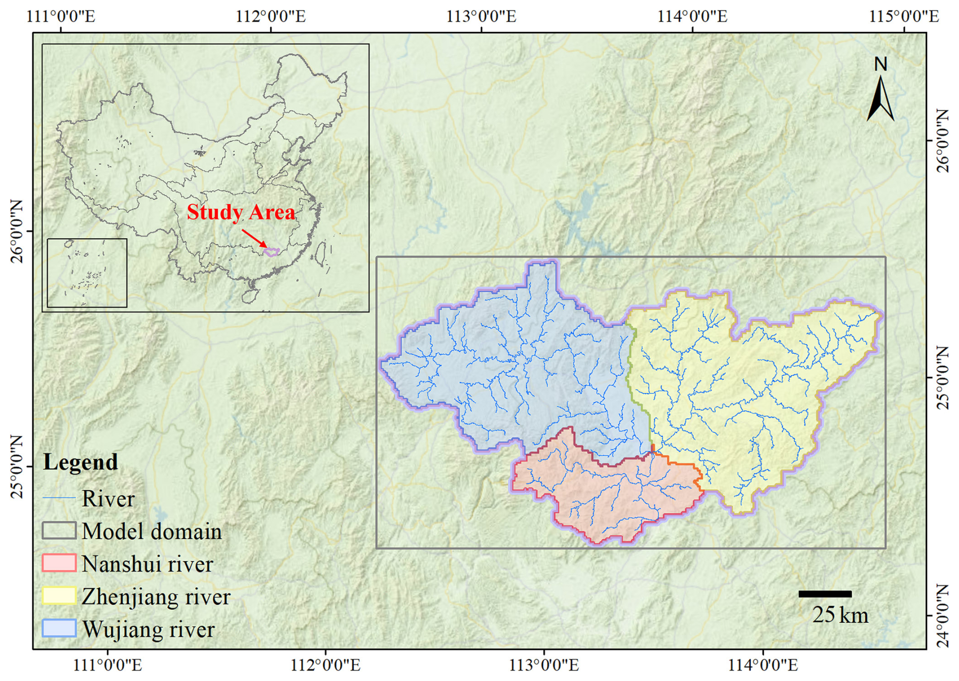
Figure 1 Model domain in the Pearl River Basin, China. The model domain encompasses three headwater watersheds, including the Zhenjiang River, Wujiang River, and Nanshui River. The domain boundary is shown in purple, and river networks are illustrated in blue. Different colors denote individual watersheds. The inset map indicates the geographic location of the study area within China.

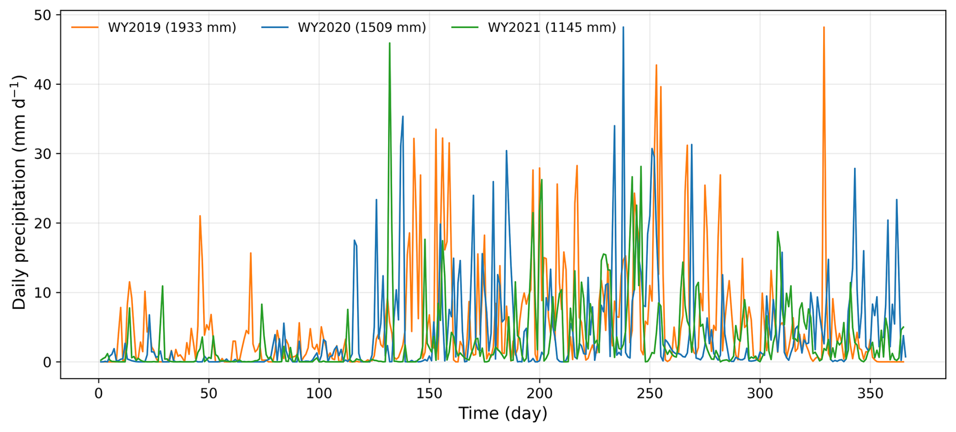
Figure 2 Daily precipitation time series aggregated from hourly data over the study region for three water years (WY2019–WY2021), used to illustrate hydroclimatic variability. Total annual precipitation is 1933 mm (WY2019), 1509 mm (WY2020), and 1145 mm (WY2021). Hourly precipitation is used in the model simulations.

Soil texture for the upper 10 layers was obtained from the GSDE global dataset (Shangguan et al., 2014), while the permeability of the bottom 100 m layer was derived from the GLHYMPS global dataset and further adjusted using an e-folding decay function with depth and slope (Gleeson et al., 2011; Fan et al., 2007). Land cover information was taken from the MODIS MCD12Q1.061 product (Friedl and Sulla-Menashe, 2022). Terrain slope was calculated from a digital elevation model (DEM) after applying hydrological processing to ensure flow connectivity (Eilander et al., 2021). Both slope and land cover datasets were adopted from the national-scale CONCN model (Yang et al., 2025a). All original datasets were reprojected and interpolated to match the model grid and resolution. Lateral and bottom boundary conditions were prescribed as no-flow boundaries.

For each watershed, the initial condition was specified with a uniform water table depth (WTD) of 2 m. The model was first driven by multi-year mean precipitation minus evapotranspiration (P−ET), derived from the national-scale CONCN model, to reach a quasi-equilibrium state, defined as a condition where the change in total water storage is less than 1 % of the cumulative P−ET over the corresponding period (Yang et al., 2025a). Subsequently, the land surface model (CoLM) was activated, and the coupled system was forced using meteorological data from water year (WY) 2019 (October–September) derived from the ERA5-Land reanalysis (Muñoz-Sabater et al., 2021) for a four-year spin-up to achieve dynamic equilibrium. The model was then driven by meteorological forcings from WY2020 and WY2021 for subsequent simulations.

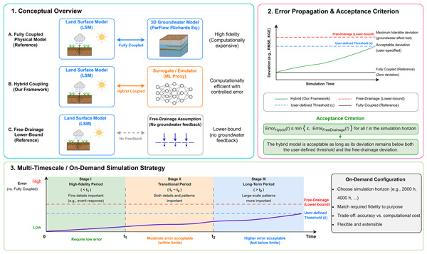
In addition, we constructed an alternative configuration (PFFD) in which lateral groundwater flow was disabled and the bottom boundary condition was changed from a no-flow boundary to a free-drainage boundary. This setup approximates the treatment of subsurface processes commonly adopted in traditional land surface models, where groundwater feedback is largely neglected. This configuration serves as a lower-bound benchmark for evaluating the hybrid coupling system (Fig. 3). Specifically, if the discrepancies between the hybrid coupling and the fully coupled physical model are not greater than those between the free-drainage configuration and the fully coupled model, it suggests that the hybrid approach is able to capture, to some extent, the influence of groundwater on land surface processes.

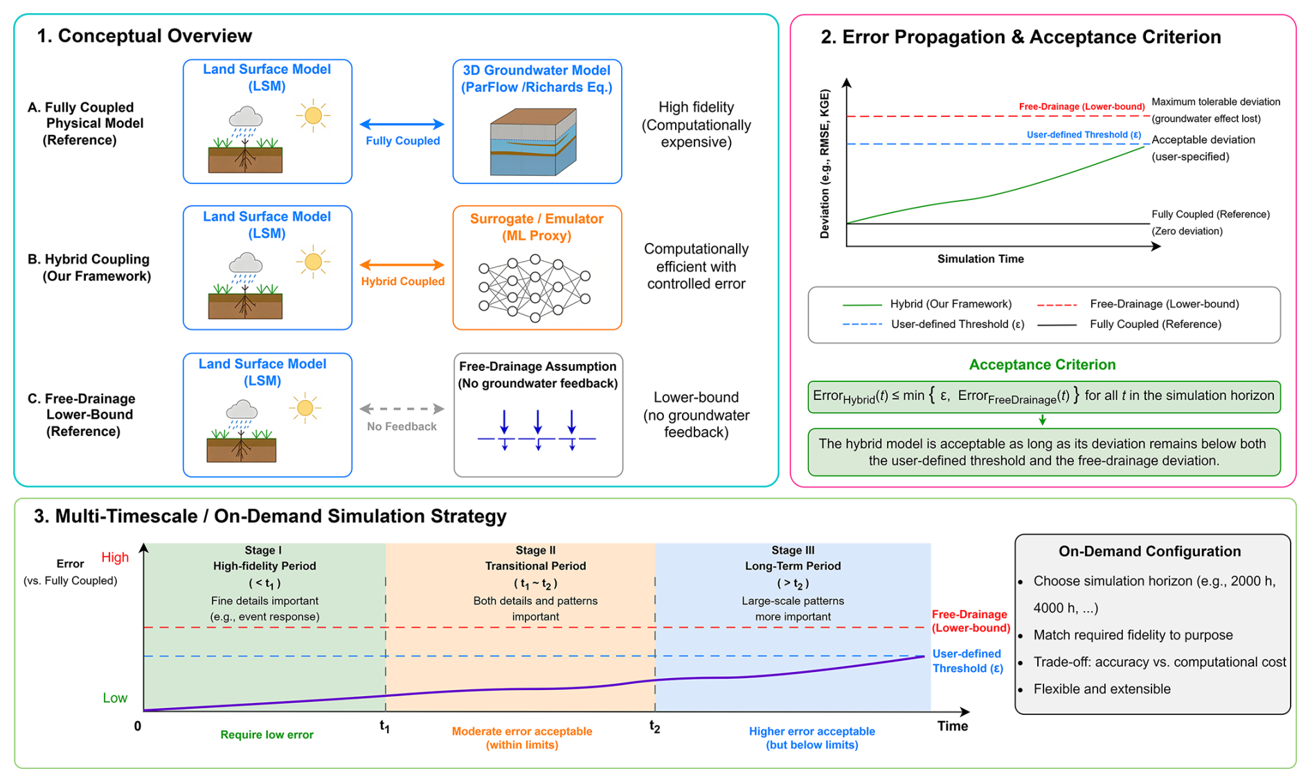
Figure 3 Conceptual framework of the hybrid groundwater–land surface coupling system. (1) Conceptual overview: comparison between the fully coupled physical model (reference), the proposed hybrid coupling using a surrogate/emulator, and the free-drainage configuration representing a lower-bound case without groundwater feedback. (2) Error propagation and acceptance criterion: deviation of the hybrid system relative to the fully coupled reference is evaluated over time. The hybrid solution is considered acceptable as long as its error remains below the free-drainage lower-bound deviation and, when specified, a user-defined threshold that is typically lower and more stringent, ensuring that essential groundwater effects are retained. (3) Multi-timescale/on-demand simulation strategy: the framework enables flexible simulation across different temporal horizons, where high fidelity is maintained for short-term dynamics, while larger errors are tolerated for long-term simulations within defined bounds, allowing a trade-off between accuracy and computational efficiency.

2.2 ParFlow deep-learning surrogate model

The ParFlow surrogate model developed in this study is a deep learning architecture adapted from FSTR (Bennett et al., 2024), itself a variant of PredRNN (Wang et al., 2023). The surrogate is designed to emulate the physics-based ParFlow model by predicting the 3D pressure head field at each timestep, given the initial pressure head, static parameters (e.g., soil properties), and dynamic external inputs (root-zone net fluxes provided by CoLM). In this study, the term “external inputs” refers specifically to root-zone net fluxes provided by the land surface model, rather than raw meteorological forcings. This choice preserves the original CoLM/ParFlow flux-exchange interface, allowing the surrogate to replace the physics-based ParFlow solver within the online coupled system; it was not introduced to improve the surrogate's predictive accuracy or autoregressive stability. For surrogate training and validation, these net fluxes were obtained from CoLM/ParFlow simulations forced by meteorological data. The resulting root-zone net fluxes were extracted and used as dynamic inputs to the surrogate model. The predicted pressure head can then be used to derive WTD and, in combination with soil hydraulic parameters, to estimate soil moisture through the van Genuchten (VG) model (van Genuchten, 1980).

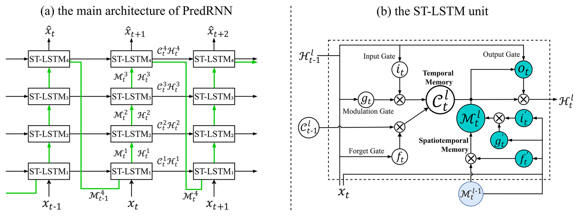
Figure 4 Architecture of the PredRNN model and the spatiotemporal LSTM (ST-LSTM) unit (Wang et al., 2023). (a) Overall architecture, illustrating the stacked ST-LSTM layers and the flow of temporal and spatiotemporal memories (${\mathcal{C}}_t^l$ and ${\mathcal{M}}_t^l$) across timesteps. (b) Structure of a single ST-LSTM unit, showing the interactions between temporal memory, spatiotemporal memory, and the gating mechanisms that control information propagation.

The core architecture of the PredRNN-based surrogate is illustrated in Fig. 4. The left panel presents the stacked spatiotemporal LSTM (ST-LSTM) structure and the spatiotemporal memory (ℳ) flow across layers and timesteps, while the right panel shows the detailed structure of a single ST-LSTM unit. The corresponding mathematical formulations of the ST-LSTM and the action-conditioned mechanism are given below. In the equations, t denotes the current timestep, and l indicates the layer index in the stacked ST-LSTM architecture. The operator ^* represents convolution, and ⊙ denotes element-wise multiplication. The terms $W_{\cdot \cdot }$ denote learnable convolutional kernels, and σ(⋅) and tanh(⋅) represent the sigmoid and hyperbolic tangent activation functions, respectively. In the action-conditioned mechanism, ${\mathcal{V}}_t^l$ can be interpreted as an action-modulated representation of the previous hidden state ${\mathcal{H}}_{t-\mathrm{1}}^l$, where the external forcing 𝒜_t−1 is incorporated to influence the state transition.

$$\begin{array}{}\text{(1)}& {\displaystyle }{g}_t=\tanh \left(W_{xg}*{\mathcal{X}}_t+W_{hg}*{\mathcal{H}}_{t-\mathrm{1}}^l\right)\text{(2)}& {\displaystyle }{i}_t=\mathit{\sigma }(W_{xi}*{\mathcal{X}}_t+W_{hi}*{\mathcal{H}}_{t-\mathrm{1}}^l)\text{(3)}& {\displaystyle }{f}_t=\mathit{\sigma }(W_{xf}*{\mathcal{X}}_t+W_{hf}*{\mathcal{H}}_{t-\mathrm{1}}^l)\text{(4)}& {\displaystyle }{\mathcal{C}}_t^l=f_t\odot {\mathcal{C}}_{t-\mathrm{1}}^l+i_t\odot g_t\text{(5)}& {\displaystyle }{g}_t{}^{\prime }=\tanh (W_{xg}{}^{\prime }*{\mathcal{X}}_t+W_{mg}*{\mathcal{M}}_t^{l-\mathrm{1}})\text{(6)}& {\displaystyle }{i}_t{}^{\prime }=\mathit{\sigma }(W_{xi}{}^{\prime }*{\mathcal{X}}_t+W_{mi}*{\mathcal{M}}_t^{l-\mathrm{1}})\text{(7)}& {\displaystyle }{f}_t{}^{\prime }=\mathit{\sigma }(W_{xf}{}^{\prime }*{\mathcal{X}}_t+W_{mf}*{\mathcal{M}}_t^{l-\mathrm{1}})\text{(8)}& {\displaystyle }{\mathcal{M}}_t^l=f_t{}^{\prime }\odot {\mathcal{M}}_t^{l-\mathrm{1}}+i_t{}^{\prime }\odot g_t{}^{\prime }\text{(9)}& {\displaystyle }\begin{array}{rl}{o}_t& =\mathit{\sigma }(W_{xo}*{\mathcal{X}}_t+W_{ho}*{\mathcal{H}}_{t-\mathrm{1}}^l+W_{co}*{\mathcal{C}}_t^l\\ & +W_{mo}*{\mathcal{M}}_t^l)\end{array}\text{(10)}& {\displaystyle }{\mathcal{H}}_t^l=o_t\odot \tanh (W_{\mathrm{1}\times \mathrm{1}}*\left[{\mathcal{C}}_t^l,{\mathcal{M}}_t^l\right])\text{(11)}& {\displaystyle }\mathrm{Action}\mathrm{fusion}:{\mathcal{V}}_t^l=(W_{hv}*{\mathcal{H}}_{t-\mathrm{1}}^l)\odot (W_{av}*{\mathcal{A}}_{t-\mathrm{1}})\text{(12)}& {\displaystyle }{\mathcal{H}}_t^l,{\mathcal{C}}_t^l,{\mathcal{M}}_t^l=\text{ST-LSTM}({\mathcal{X}}_t,{\mathcal{V}}_t^l,{\mathcal{C}}_{t-\mathrm{1}}^l,{\mathcal{M}}_t^{l-\mathrm{1}})\end{array}$$

Building upon the standard PredRNN formulation, we introduce several modifications following FSTR to enable its application as a surrogate model. Specifically, separate convolutional encoders are employed to process static parameters and the initial pressure head field, which are used to initialize both the temporal memory 𝒞 and the spatiotemporal memory ℳ, respectively. The static inputs are constructed from hydrogeological parameters across all vertical layers. Specifically, four soil parameters – permeability, porosity, and the van Genuchten parameters (α and n) – are included for each of the 11 layers, resulting in 44 channels. In addition, two surface-related parameters, slope and Manning's coefficient, are incorporated, yielding a total of 46 static input channels. These parameters are encoded once and used to initialize the memory states (𝒞) of the network.

Following FSTR, we adopt an autoregressive scheme in which the predicted pressure head field from the previous timestep is directly used as the input 𝒳_t for the next timestep. This design avoids the use of scheduled sampling in PredRNN, where ground-truth and predicted states are mixed during training (Wang et al., 2023). External inputs are incorporated through the action-conditioned design in PredRNN. In this study, the actions correspond to root-zone net fluxes provided by the physics-based CoLM/ParFlow model (Sect. 2.1), representing the combined effects of infiltration and evapotranspiration. By adopting this flux-based interface, the surrogate model remains consistent with the input–output structure of the ParFlow model, enabling seamless coupling with the land surface model. During coupled simulations, fluxes computed by CoLM can be directly supplied to the surrogate model, allowing it to advance subsurface states in a manner consistent with the original physics-based system. This differs from the original FSTR formulation, where the surrogate is trained in an end-to-end manner using meteorological forcings as inputs.

Additional adaptations were made to account for structural differences between the earlier ParFlow-CLM configuration used in FSTR and the updated version applied in this study. Specifically, the new CoLM/ParFlow model includes 10 coupled layers, resulting in input channel dimensions of 11, 10, and 46 for the initial condition, external inputs, and static parameters, respectively, compared with 5, 5, and 15 in FSTR. Despite the increased input dimensionality, we retain the original hidden-state size of 16 channels used in FSTR, rather than increasing the hidden-state dimensionality of the ST-LSTM layers. This design implicitly requires the network to encode high-dimensional inputs into a compact latent representation. In addition, while FSTR used a convolutional kernel size of 5, we found that a kernel size of 3 yields better performance in our experiments. This improvement may be related to the characteristic spatial correlation scales of groundwater dynamics. These design choices improve predictive performance while substantially reducing the number of trainable parameters. As a result, the final model contains approximately 86 K trainable parameters, less than half that of the original FSTR model (194 K parameters).

The model was trained using data from WYs 2019–2020, while the first 720 h of WY2021 were used for validation, and the remaining 8040 h (hours 721–8760) were used for subsequent evaluation. The model domain was partitioned into non-overlapping patches of size 16 × 16. For domains where the spatial dimensions are not exact multiples of the patch size, additional patches were extracted from the domain boundaries to ensure full spatial coverage. A rollout horizon of 120 h was employed without overlap for training and validation, yielding 23 360 training samples and 960 validation samples. This horizon was chosen to balance temporal dependency learning and computational cost. The model predicts pressure head fields at the patch level, which are then reassembled to reconstruct the full domain.

Model training was conducted using the AdamW optimizer with a OneCycle learning rate schedule. The learning rate increased from 4 × 10⁻⁴ to 2 × 10⁻³ during the first 30 % of training, and then decreased to 8 × 10⁻⁵ for the remaining iterations. A batch size of 16 was used. The loss function consists of a mean squared error (MSE) term between the predicted and reference pressure head fields and an additional penalty on the horizontal gradients of the predicted pressure head field, with a weighting factor of 0.1, to enforce spatial smoothness. Static parameters were standardized using their spatial mean and standard deviation for each vertical layer. Pressure heads were standardized using the mean and standard deviation computed from the two-year training period for each vertical layer. Net fluxes were standardized using the mean and standard deviation computed from the same training period. The implications of layer-wise standardization for vertical hydraulic gradients, including their representation under dry and saturated conditions, are discussed in the Supplement (Sect. S1 and Figs. S1–S3). Training was performed for 8 × 10⁴ iterations (about 55 epochs). To assess the influence of stochastic variability, the training process was repeated five times. In two of these runs, training was further continued for an additional 8 × 10⁴ iterations at a fixed learning rate of 8 × 10⁻⁵; however, no significant improvement in loss was observed. The model with the best validation performance was selected for subsequent evaluation. All experiments were conducted on a single NVIDIA A100 GPU (80 GB).

2.3 Additional architectural experiments

We also examined a temporal self-attention module to assess whether it could improve the surrogate's representation of long-term dependencies; architectural details are provided in Sect. S2. Preliminary experiments with the attention-enhanced architecture (Fig. S4) showed performance comparable to that of the baseline model in terms of both training loss and validation RMSE. This indicates that the PredRNN-based architecture already captures the dominant spatiotemporal dependencies in this application, leaving limited room for further improvement through additional attention modules. Given that the primary objective of this study is to demonstrate the feasibility of coupling the ParFlow surrogate with the physics-based CoLM model, we did not pursue further architectural refinements. Nevertheless, future work may explore alternative architectures, such as transformer-based models, for broader applications.

2.4 ParFlow surrogate–CoLM physics hybrid coupling

The trained ParFlow surrogate was coupled with the physics-based CoLM in an online hybrid framework to reproduce the behavior of the fully physics-based coupled system. In this framework, CoLM and the surrogate exchange information dynamically at every timestep: CoLM provides root-zone net fluxes, and the surrogate predicts the updated three-dimensional pressure head field. Saturation is subsequently derived from the predicted pressure head through the van Genuchten (VG) relationship. Both the updated pressure head and the derived saturation are then passed back to CoLM for the next timestep. To enable this two-way coupling, the standalone surrogate was reformulated from a multi-step predictor driven by prescribed net fluxes to a single-step autoregressive model. At each timestep, the surrogate takes the current subsurface state together with the corresponding CoLM-generated net fluxes and advances the pressure head field by one step. This modification allows the surrogate to be embedded directly within the online coupling loop, ensuring synchronous state updates between the two components.

From an implementation perspective, CoLM was compiled as a shared library and exposed through a Fortran–C interface using BIND(C), which provides a C-compatible entry point for its land surface routines. This interface allows the compiled library to be directly invoked from external Python code during online coupling. It forms the foundation of the hybrid implementation, enabling seamless integration of CoLM physics within the surrogate prediction loop. To preserve consistency with the original physics-based coupled model and to enable a fair assessment of computational efficiency, the CoLM component retained the same domain decomposition strategy as the fully physics-based system. In the physics-based model, the domain is partitioned according to its parallel spatial decomposition, which depends on both the domain size and the number of subdivisions specified in each horizontal direction. For example, the model domain is divided into 4 partitions along the x-direction and 3 along the y-direction, resulting in 12 spatial blocks and thus 12 parallel processes.

Based on this block structure, parallel execution was implemented in Python by assigning each block to a dedicated worker process. Each worker loaded an independent CoLM shared-library instance and advanced the land surface calculations for its assigned block. Within each worker, meteorological forcings were loaded one day at a time and cached locally to reduce repeated I/O overhead, while still being applied at the native hourly timestep during simulation. The surrogate, by contrast, operates on fixed-size spatial patches (16 × 16) consistent with its training configuration. After each timestep, the block-wise CoLM outputs were first assembled back to the full domain and then reshaped into surrogate input patches for the next prediction step. The hybrid system was evaluated over the remaining 8040 h of WY2021 (hours 721–8760), following surrogate training on water years 2019–2020 and validation over the first 720 h of WY2021. This setup allows evaluation of both predictive performance and long-term stability of the coupled system under realistic forcing conditions.

3 Results and discussion

3.1 Training robustness and computational efficiency

To assess training robustness, the surrogate model was trained five times using the same random seed and otherwise identical training settings (Fig. S5). All runs showed a similar optimization pattern, with a rapid decrease in both training loss and validation RMSE during the early stage, followed by gradual convergence to similar plateau levels. At the same time, the trajectories were not identical: some runs exhibited more pronounced intermediate fluctuations, particularly in validation RMSE. Controlled tests identified nondeterministic GPU backpropagation associated with the reflection-padding operation used in the network as a source of this variability. For two of these runs, training was further extended beyond 8 × 10⁴ iterations at a fixed learning rate of 8 × 10⁻⁵, but this resulted in little additional improvement in validation performance, indicating that the model had effectively converged. The first run (Job 2680 in Fig. S5) was selected because it was among the three runs with similarly low validation RMSE and was not outperformed by the subsequent runs. Its checkpoint at 8 × 10⁴ iterations was used for the subsequent evaluation. A sensitivity analysis using the checkpoints at 7 × 10⁴ and 7.5 × 10⁴ iterations from the same run produced very similar results, indicating limited sensitivity to checkpoint selection over this late-training interval (Sect. S3 and Figs. S6–S8).

In terms of computational efficiency, five repeated timing tests were conducted for both the fully physics-based coupled model and the hybrid coupled model over the 720 h period designated as Segment 9 in the segment-based hydrological analysis presented in Sect. 3.2. All tests were performed on a dual-socket compute node equipped with two 96-core AMD EPYC 9654 processors and one NVIDIA A100-SXM4-80GB GPU, providing 192 physical CPU cores and 384 hardware threads in total. The fully physics-based coupled model used 12 MPI processes, consistent with the 4 × 3 spatial decomposition described in Sect. 2.4, whereas the hybrid coupled model used the GPU for surrogate inference and 12 Python worker processes for the CoLM component corresponding to the same spatial decomposition.

The wall-clock times of the fully physics-based model were 5087, 5569, 5626, 7276, and 4914 s, whereas those of the hybrid model were 339, 261, 257, 393, and 311 s, respectively. The corresponding mean runtimes were 5694.4 and 312.2 s, indicating an average speedup of 18.24× for the hybrid coupled model. Further optimization (e.g., implementation-level improvements) could potentially lead to additional gains, but this is beyond the scope of the present study. Because computational performance can vary with the computing environment and the hydrological conditions represented by the simulated period, these timing results should be regarded as representative benchmarks rather than a universal speedup factor. The reported timings do not include the preceding standalone ParFlow spin-up. For a newly established basin model, spin-up represents a one-time upfront cost and does not need to be repeated in subsequent simulations using the same model configuration. When an equilibrated large-scale modeling framework is already available, such as CONCN, its model state can be used to initialize the regional application, thereby avoiding a separate steady-state spin-up and leaving only the transient coupled spin-up.

3.2 Performance of the hybrid coupled system

The 8040 h continuous simulation (hours 721–8760 of WY2021) provides an initial assessment of the temporal evolution and spatial variability of WTD errors under autoregressive prediction (Fig. 5). Overall, the median WTD bias remains relatively small throughout the simulation, generally staying within ∼ 0.5 m, indicating that the hybrid model maintains a reasonable level of accuracy over time. However, the median bias increases gradually, suggesting a progressive accumulation of errors during the autoregressive prediction. At the same time, the spread of the bias distribution widens substantially: the interquartile range (25 %–75 %) expands from near-zero at the beginning to approximately 0.2–1.0 m, while the 10 %–90 % range grows to over ∼ 2 m in the later stages, reflecting increasingly dispersed errors in the hybrid system. Notably, pronounced expansions of the bias range often coincide with changes in precipitation forcing, during which both the median and upper quantiles exhibit sharper excursions. This qualitative correspondence suggests a possible relationship between precipitation forcing and the spatial spread of model errors, motivating a more quantitative analysis.

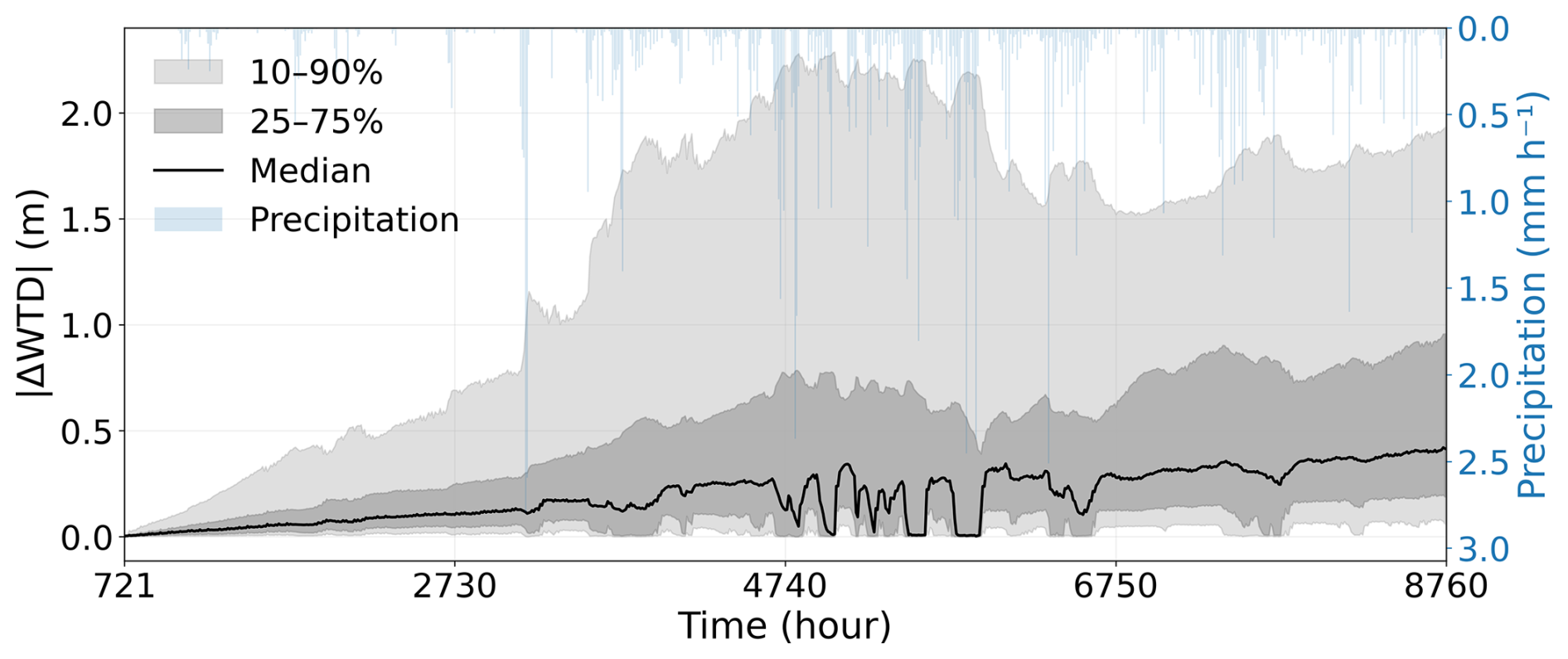
Figure 5 Temporal evolution of water table depth (WTD) bias and its variability over the 8040 h evaluation period (hours 721–8760 of WY2021). The black line represents the median absolute WTD bias across all grid cells at each time step, while the shaded regions denote the interquartile range (25 %–75 %) and the broader distribution (10 %–90 %), respectively. The blue curve (right axis) shows precipitation, providing the primary external forcing to the system.

Therefore, following the approach of Huang et al. (2026), we quantified this relationship using 12 separately initialized 720 h segment simulations (Fig. S9). For each segment, the spatial mean, median, 75th percentile, and 90th percentile of absolute WTD bias were summarized using both their time-averaged and final-hour values and correlated with the segment-mean precipitation and within-segment precipitation variability, represented by its standard deviation (Table S1). The spatial mean and median errors showed relatively weak relationships with either precipitation metric, whereas substantially stronger correlations were found for the upper quantiles, particularly the time-averaged 75th-percentile error. Its correlations with precipitation variability (Pearson r=0.944; Spearman ρ=0.902) were slightly stronger than those with mean precipitation (r=0.865; ρ=0.881). More generally, the time-averaged upper-quantile errors were more strongly related to precipitation characteristics than their final-hour counterparts. These results do not imply that greater precipitation necessarily produces larger prediction errors. Rather, the stronger relationships with precipitation variability are consistent with greater model sensitivity to fluctuating hydrological forcing and associated wet–dry transitions, which preferentially broaden the upper part of the spatial error distribution.

The spatial distributions of WTD, soil moisture, and latent heat exhibit clear patterns controlled by underlying physical factors (Fig. 6). WTD shows strong topographic control, with shallow water tables concentrated along river networks and valley bottoms, and deeper groundwater levels distributed over upland regions. Soil moisture broadly follows this pattern, reflecting the influence of groundwater proximity on near-surface water availability. At the same time, soil moisture and latent heat are additionally modulated by soil texture and land surface properties, leading to finer-scale spatial heterogeneity beyond the topographic signal. In particular, variations in soil hydraulic properties and vegetation-related processes introduce spatial variability that is not solely explained by groundwater dynamics (Fig. S10).

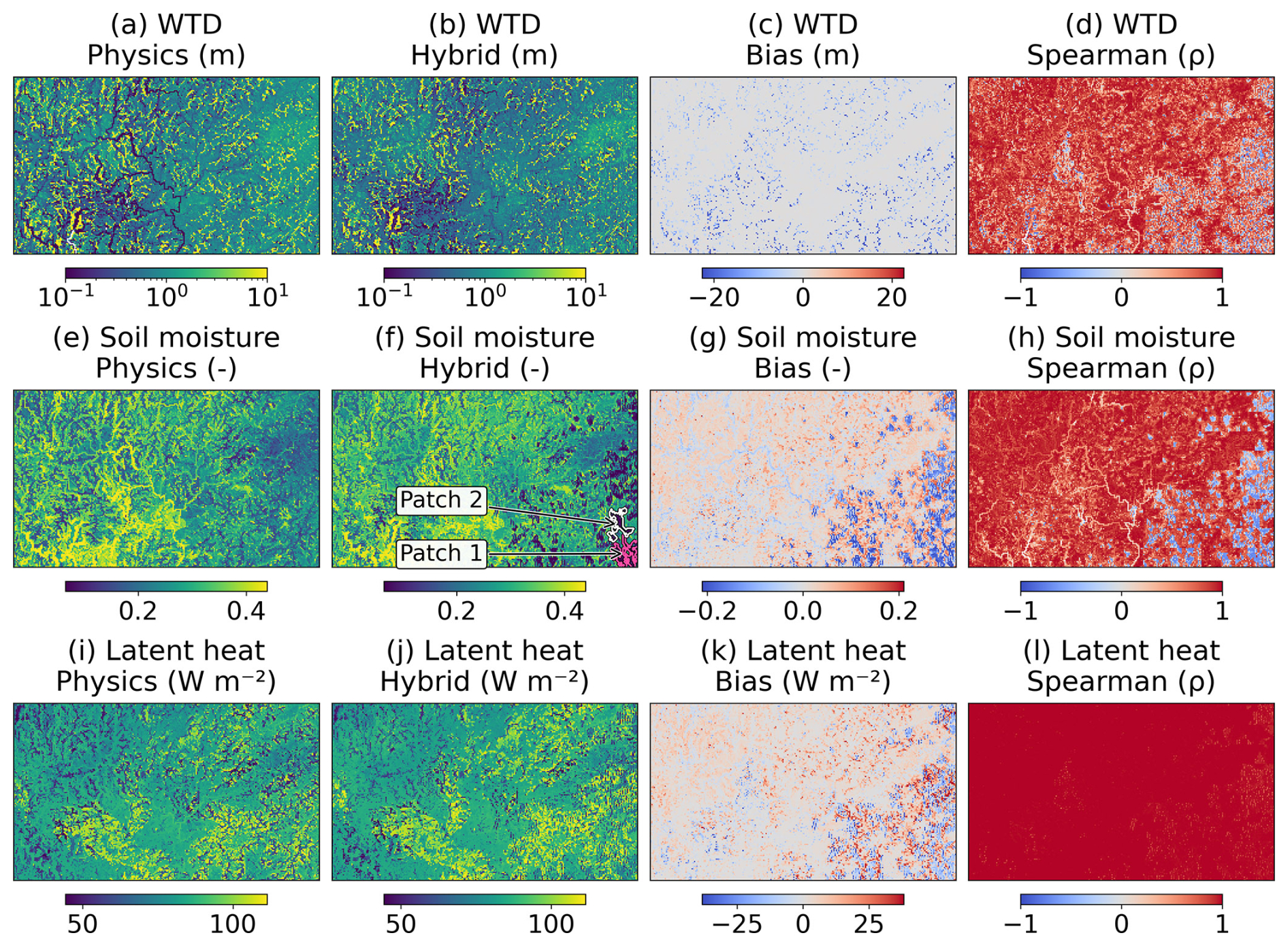
Figure 6 Spatial distributions of mean states over the 8040 h evaluation period (hours 721–8760 of WY2021) and corresponding model agreement between the physics-based and hybrid models. The first, second, and third rows correspond to water table depth (WTD), near-surface soil moisture (top layer), and latent heat flux, respectively. For each variable, the columns show: (a, e, i) the physics-based model, (b, f, j) the hybrid model, (c, g, k) the bias, and (d, h, l) the Spearman rank correlation coefficient (ρ) computed from the temporal series at each grid cell. The bias is defined as hybrid minus physics, such that positive values indicate overestimation by the hybrid model relative to the physics-based model, and negative values indicate underestimation. Spearman correlation quantifies the temporal agreement between the two models at each grid cell, with values close to 1 indicating strong monotonic consistency. The magenta and white contours in panel (f) delineate Patch 1 and Patch 2, respectively, defined as the two largest contiguous dry-bias regions used in the localized analysis.

The hybrid model reproduces the overall spatial patterns of all three variables well, indicating that it successfully captures the dominant large-scale controls. However, noticeable discrepancies appear in certain regions, particularly in the southeastern part of the domain, where both WTD and soil moisture exhibit localized distortions compared to the physics-based model. These inconsistencies propagate into the latent heat flux, resulting in larger biases in the same region. Consistent with these spatial deviations, the temporal agreement between the hybrid and physics-based models, as measured by the Spearman correlation, is slightly reduced in these areas. This suggests that errors in subsurface states can propagate upward, affecting both the magnitude and timing of surface fluxes.

To further examine the localized deterioration in the southeastern part of the domain, we analyzed the two largest contiguous dry-bias patches outlined in Fig. 6. As a descriptive onset criterion, we defined patch emergence as the first occurrence of 72 consecutive hours with a patch-mean surface pressure-head bias below −0.5 m. On a common WY2021 time axis, the two patches emerged at hours 3246 and 3248 in the simulation initialized at hour 1, compared with hours 3207 and 3347 in the simulation initialized at hour 721. Their broadly similar calendar timing, despite the 720 h difference in initialization, indicates that elapsed simulation time alone cannot explain their development. Smaller negative biases had already emerged during the relatively dry January period, whereas the more pronounced departures followed a substantial rainfall event on 9–10 February (hours 3145–3192), which delivered approximately 48–51 mm over the two patches. This sequence is consistent with accumulated errors being amplified during a dry-to-wet transition, although temporal proximity does not establish causality. Compared with nearby areas exhibiting smaller errors, the two patches were characterized by steeper slopes and lower aquifer permeability and porosity, while experiencing broadly similar meteorological forcing. These local properties may have increased their susceptibility to persistent deviations under changing moisture conditions. Taken together, the results suggest that progressive error accumulation, modulated by wet–dry transitions and local terrain and subsurface properties, provides a plausible explanation for the spatially concentrated deterioration, rather than identifying any single factor as its cause.

As a complementary evaluation of surface-water behavior, we also examined domain-wide surface-water storage and streamflow at two representative locations. The hybrid model captured the main surface-water responses, particularly over shorter prediction windows, whereas agreement deteriorated as autoregressive errors accumulated during the continuous simulation. Detailed results are provided in the Supplement (Sect. S4 and Figs. S11–S12).

The central objective of this study is to provide a computationally efficient approach for representing three-dimensional groundwater dynamics and their interactions with land-surface processes within Earth system modeling, rather than to develop a standalone surrogate that must reproduce CoLM/ParFlow exactly over an unrestricted prediction horizon. Because errors are expected to accumulate during continuous autoregressive prediction, the framework introduced in Fig. 3 defines an application-dependent acceptance criterion. CoLM/ParFlow serves as the fully physics-based reference, whereas PFFD represents a lower-bound benchmark in model fidelity, in which lateral groundwater flow and the associated groundwater feedback are largely absent. Accordingly, the hybrid solution is considered to retain meaningful groundwater–land-surface interactions as long as its deviation from CoLM/ParFlow remains smaller than the PFFD–CoLM/ParFlow deviation and, when specified, below a user-defined error threshold. The domain-averaged latent heat flux provides an integrated measure for evaluating the hybrid system within this framework (Fig. 7a, b).

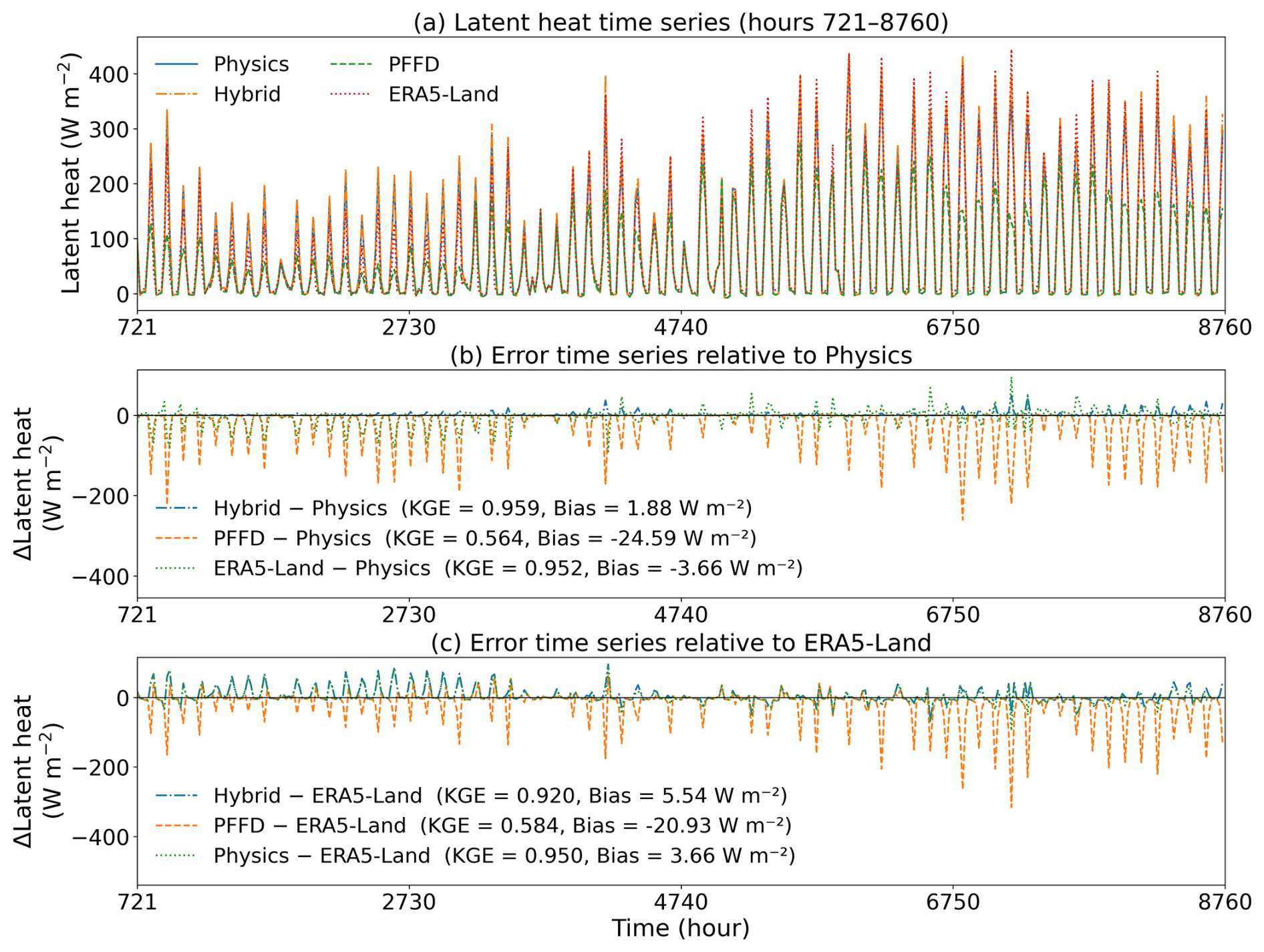
Figure 7 Comparison of domain-averaged latent heat flux across different modeling configurations and references. (a) Latent heat flux time series over the 8040 h evaluation period (hours 721–8760 of WY2021) from the physics-based model, the hybrid model, the free-drainage (PFFD) configuration, and the ERA5-Land reanalysis. (b) Error time series relative to the physics-based model (Hybrid – Physics, PFFD – Physics, and ERA5-Land – Physics). (c) Error time series relative to ERA5-Land (Hybrid – ERA5-Land, PFFD – ERA5-Land, and Physics – ERA5-Land). To improve readability, the time series is subsampled and plotted at 20 h intervals.

Over the 8040 h evaluation period, the hybrid model closely follows the latent heat dynamics of the fully physics-based simulation, achieving a KGE of 0.959 and a mean bias of 1.88 W m⁻² relative to CoLM/ParFlow. By contrast, PFFD systematically underestimates latent heat flux, particularly during high-flux periods, resulting in a substantially lower KGE of 0.564 and a mean bias of −24.59 W m⁻². Its negative bias is also evident in the spatial comparison, which shows broadly reduced latent heat flux across the domain (Fig. S13). Although PFFD retains some of the general temporal variability, its substantially larger magnitude errors demonstrate the effect of omitting groundwater feedback. The much smaller Hybrid–CoLM/ParFlow discrepancy therefore satisfies the acceptance criterion defined above and indicates that the hybrid system retains the key groundwater–land-surface interactions represented by the fully physics-based model. In this demonstration, no additional numerical threshold was imposed beyond the PFFD-based benchmark, although users may specify a more restrictive error tolerance according to their application requirements. For other applications, users could set tolerances for WTD error statistics or domain-averaged latent heat flux error, with the metric and its spatial and temporal aggregation chosen according to the intended use.

Because CoLM/ParFlow is itself a model-based reference, ERA5-Land was additionally included as an external, observation-informed reference. ERA5-Land is driven by atmospheric forcing from ERA5, which is constrained by observations through a global data assimilation system, and therefore provides a useful consistency check on the large-scale latent heat dynamics. Using ERA5-Land as the common reference (Fig. 7c), CoLM/ParFlow shows strong agreement, with a KGE of 0.950 and a mean bias of 3.66 W m⁻². The hybrid model retains a comparable level of consistency, with a KGE of 0.920 and a mean bias of 5.54 W m⁻², whereas PFFD exhibits substantially poorer agreement, with a KGE of 0.584 and a mean bias of −20.93 W m⁻². The closer agreement of both CoLM/ParFlow and the hybrid model with ERA5-Land, relative to PFFD, provides complementary support for the importance of retaining groundwater feedback in representing large-scale latent heat flux. The ERA5-Land–CoLM/ParFlow difference is also shown in Fig. 7b using CoLM/ParFlow as the common reference, allowing its magnitude to be compared directly with the Hybrid–CoLM/ParFlow and PFFD–CoLM/ParFlow deviations on a consistent basis.

3.3 Propagation of groundwater errors to land-surface fluxes

The temporal analysis (Figs. 5 and 7) suggests a clear co-variation between subsurface and surface errors. In particular, periods with larger WTD biases – such as around hour ∼ 4380 and after hour ∼ 6570 – are consistently associated with amplified deviations in latent heat flux, indicating a potential propagation of errors from groundwater states to surface fluxes. However, domain-averaged time series cannot fully capture the spatial variability of this relationship. To further examine how groundwater-related errors are associated with flux biases, we extend the analysis to the grid-cell level by analyzing the joint distribution of WTD and latent heat errors.

To characterize the relationship between groundwater-related errors and their propagation to surface fluxes, we constructed a paired dataset by comparing the hybrid model outputs against the fully physics-based CoLM/ParFlow simulations over the 8040 h evaluation period (hours 721–8760 of WY2021). At each grid cell and timestep, WTD and latent heat flux differences were computed, yielding ΔWTD and ΔLatent heat. These paired samples were collected across randomly sampled timesteps and grid cells and combined into a dataset spanning the entire domain and evaluation period. The relationships were analyzed using binned boxplots to characterize the distribution of errors under different WTD and WTD-errors conditions (Fig. 8). Results show that WTD bias increases systematically with increasing WTD (Fig. 8a), indicating reduced model accuracy under deeper water table conditions. In addition, latent heat bias exhibits a positive relationship with WTD bias over the intermediate error range (Fig. 8b), suggesting that errors in subsurface states may propagate upward and be amplified in surface fluxes. A complementary comparison of latent heat errors against physics-based WTD (Fig. 8c) further illustrates how surface flux errors vary across groundwater depth conditions.

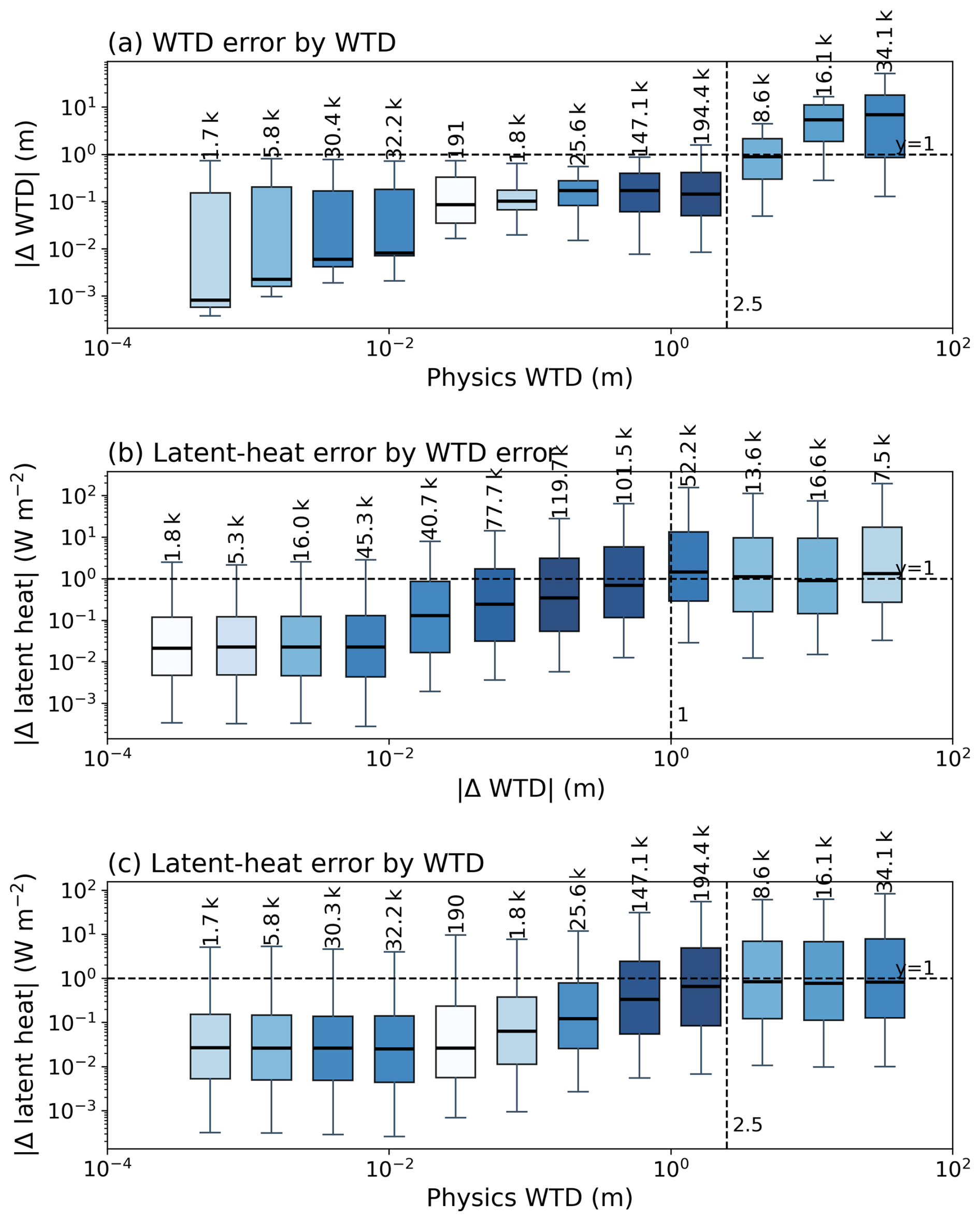
Figure 8 Boxplots showing (a) absolute WTD error as a function of physics-based WTD, (b) absolute latent heat error as a function of absolute WTD error, and (c) absolute latent heat error as a function of physics-based WTD. Boxes show the interquartile range, center lines indicate medians, whiskers span the 5th–95th percentiles, and labels give sample counts. Darker boxes indicate higher sample density. Horizontal dashed lines mark error magnitudes of 1 m in (a) and 1 W m⁻² in (b) and (c); vertical dashed lines mark physics-based WTD of 2.5 m in (a) and (c) and absolute WTD error of 1 m in (b).

Most samples are concentrated in the relatively shallow groundwater and small WTD-error ranges (Fig. 8a, b). As shown in Fig. 8b, the median latent heat errors in the more densely populated WTD-error bins generally remain below 1 W m⁻², indicating relatively small errors for typical samples. However, the upper portions of the error distributions extend to substantially larger values, approaching 100 W m⁻² in some cases. Figure 8b reveals a nonlinear relationship between WTD and latent heat errors. At very small WTD errors (approximately 10⁻³–10⁻² m), latent heat errors remain relatively stable, possibly because the subsurface deviations are too small to produce a clearly distinguishable contribution to surface flux errors. Over the intermediate range of approximately 10⁻² to 1 m, latent heat errors increase markedly, broadly following a power-law relationship. At larger WTD errors (above approximately 1 m), their growth becomes less pronounced. Similarly, Fig. 8c shows that latent heat errors increase with physics-based WTD before tending to level off under deeper groundwater conditions.

These patterns may be interpreted in the context of the critical depth theory of groundwater–land surface interactions (Kollet and Maxwell, 2008; Yang et al., 2020). Under shallow groundwater conditions, where capillary connections may remain active, WTD errors can be associated with relatively large surface flux deviations. As groundwater becomes deeper, groundwater–land surface feedback generally weakens, which may partly explain why latent heat errors do not continue increasing at the same rate despite larger WTD errors. Together, these results suggest that the propagation of subsurface errors to surface fluxes is nonlinear and depends partly on groundwater depth conditions, with relatively small typical errors but potentially large deviations in a subset of samples.

3.4 Continuous versus segmented prediction

Following the application strategy outlined in Fig. 3, we examined how the fidelity of the hybrid model changes as errors accumulate during the 8040 h continuous simulation. This stage-wise analysis helps determine how long the surrogate can be run before its error exceeds the level acceptable for a particular application. We divided the evaluation period into three stages: early (hours 721–2500), middle (hours 2501–6000), and late (hours 6001–8760), and evaluated the spatial evolution of near-surface soil moisture (Fig. 9), WTD (Fig. S14), and latent heat flux (Fig. S15). During the early stage, the hybrid model closely matches the physics-based simulation, successfully capturing both large-scale spatial patterns and fine-scale heterogeneity, indicating an accurate representation of groundwater–land surface coupling. In the middle stage, deviations begin to emerge, particularly in localized regions such as the southeastern part of the domain. While the overall spatial pattern remains consistent with the physics-based model, fine-scale structures are partially degraded, suggesting that accumulated subsurface errors start to influence surface variables. By the late stage, this degradation becomes more pronounced: the hybrid model largely preserves dominant large-scale patterns, while fine-scale spatial variability is substantially reduced. Correspondingly, the Spearman correlation decreases in affected regions, indicating reduced temporal consistency.

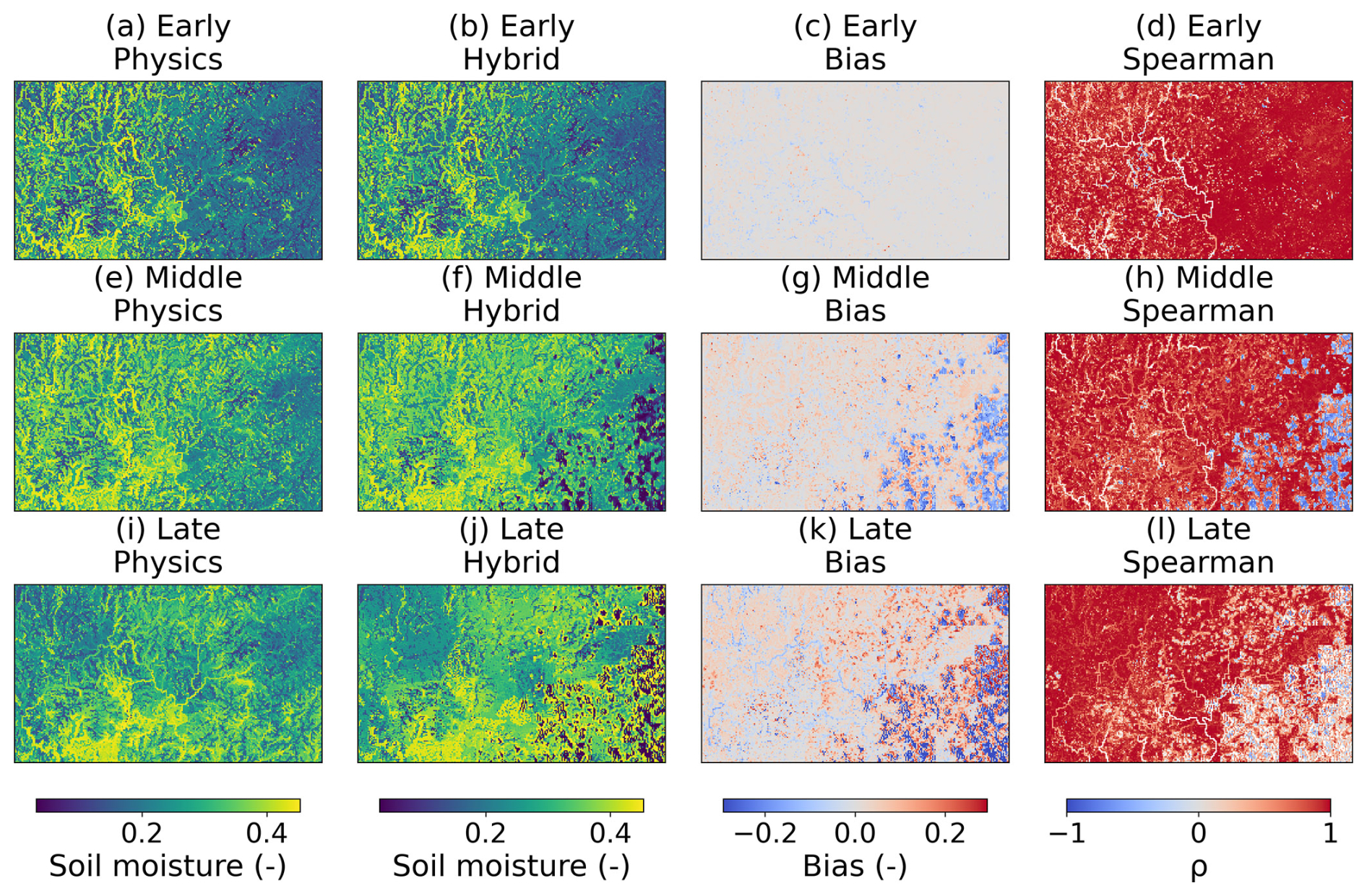
Figure 9 Temporal evolution of spatial patterns of near-surface soil moisture and model agreement across different prediction stages. Three periods are shown: early (hours 721–2500), middle (hours 2501–6000), and late (hours 6001–8760) stages of the simulation. For each period, columns represent the physics-based model, the hybrid model, the bias (Hybrid – Physics), and the Spearman correlation coefficient (ρ), respectively.

This progressive deterioration coincides with changing precipitation conditions. Consistent with the preceding quantitative analysis (Table S1), upper-tail errors are related to both segment-mean precipitation and precipitation variability, with a stronger association observed for precipitation standard deviation. This pattern suggests that wet–dry variability may contribute to error amplification, but it does not imply that precipitation alone determines error growth. Although the overall magnitude of errors may temporarily decrease during certain periods, as also indicated by the temporal analysis in Fig. 5, the spatial error structure does not fully recover. Thus, while the system may exhibit transient stabilization in an aggregated sense, the underlying spatial organization of errors remains altered. In the context of the application strategy presented in Fig. 3, these results suggest that the effective prediction horizon depends on the level of detail required: shorter prediction windows are better suited for resolving fine-scale groundwater dynamics, whereas longer simulations can still capture the dominant large-scale feedback patterns despite the loss of spatial detail.

To distinguish whether the late-stage deterioration in the continuous simulation reflects accumulated autoregressive errors or an intrinsic inability of the hybrid model to represent hydrological responses under challenging forcing, we conducted a targeted segmented prediction for Segment 9. This experiment also evaluates a practical application strategy in which the hybrid model is initialized close to the target period to reduce the influence of errors accumulated beforehand. Segment 9 was selected because it exhibits the strongest precipitation variability among the evaluated segments (Fig. S9). Despite this highly variable forcing, the segmented hybrid prediction remains closely consistent with the physics-based simulation (Fig. 10). In particular, the domain-averaged latent heat flux achieves a KGE of 1.000 relative to the physics-based model, substantially higher than that of the free-drainage configuration (0.683). Compared with the continuous autoregressive simulation, WTD error growth is greatly constrained in this segment. In the continuous run, the median WTD bias increases to about 0.3–0.4 m by this stage, with the 25 %–75 % range approaching roughly 0.8–1.0 m and the 10 %–90 % range extending to around 2 m or more. By contrast, under segmented prediction in Segment 9, the median WTD bias remains below about 0.1 m throughout the 720 h window, the interquartile range is largely confined to about 0.1–0.2 m, and even the 10 %–90 % range remains below about 0.4 m. Thus, shortening the prediction horizon substantially suppresses the error amplification observed in the continuous simulation.

Figure 10 Error evolution and flux consistency during a representative period (Segment 9; hours 5761–6480). (a) Temporal evolution of water table depth (WTD) bias in the hybrid model, shown as the median and percentile ranges (25 %–75 % and 10 %–90 %) across the domain, together with spatially averaged precipitation (inverted axis). (b) Domain-averaged latent heat flux from the physics-based model, the hybrid model, the free-drainage configuration (PFFD), and the ERA5-Land reanalysis. Kling–Gupta efficiency (KGE) values are computed with respect to the physics-based model.

The spatial fields provide consistent evidence (Fig. 11). Under segmented prediction, the hybrid model reproduces not only the dominant large-scale organization but also much of the fine-scale structure in WTD, soil moisture, and latent heat. Biases remain spatially scattered rather than coherently organized into large, distorted regions, and the Spearman correlation remains uniformly high across most of the domain. This is especially notable in comparison with the corresponding period of the continuous simulation, in which fine-scale heterogeneity is substantially degraded and localized regions of reduced agreement become clearly visible. Together, these results support the interpretation that the late-stage degradation in the continuous simulation arises primarily from cumulative error growth rather than an intrinsic inability of the hybrid model to represent the hydrological conditions occurring during Segment 9. From an application perspective, initializing the hybrid model close to a target period and limiting the prediction horizon provide a practical strategy for retaining fine-scale accuracy. A 720 h (∼ 1 month) prediction window may provide practical benefits for event-oriented applications, including flood and drought studies, depending on their specific temporal and accuracy requirements. The recovery of predictive skill after reinitialization also suggests that future integration with data assimilation could periodically correct accumulated state errors and extend the effective prediction horizon.

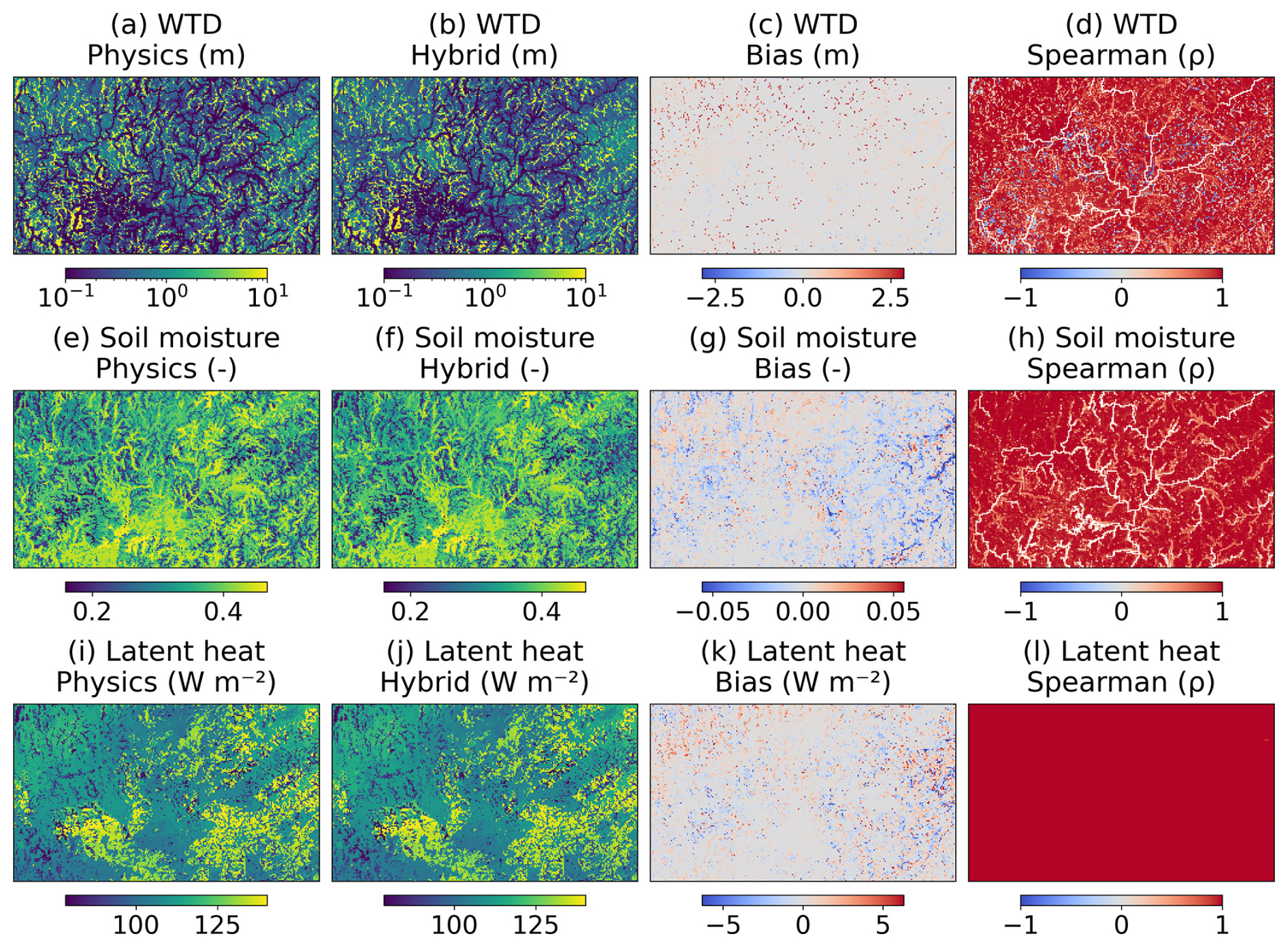
Figure 11 Spatial performance of the hybrid model under segmented prediction during a high-variability period (Segment 9; hours 5761–6480). The segment corresponds to a period with the largest precipitation variability. Rows show water table depth (WTD), soil moisture, and latent heat, respectively, while columns represent the physics-based model, the hybrid model, the bias (Hybrid – Physics), and the Spearman correlation coefficient (ρ).

4 Conclusions

Three-dimensional groundwater dynamics play a critical role in regulating land–atmosphere interactions through subsurface–surface feedbacks, yet resolving variably saturated flow using the Richards' equation at large scales remains computationally prohibitive. In this study, we developed a hybrid coupling framework in which a deep learning surrogate replaces the physics-based groundwater solver while preserving the original coupling interface. This design substantially reduces computational cost and provides a practical pathway for representing three-dimensional groundwater dynamics in land surface and Earth system models.

The proposed framework was demonstrated in a representative watershed system in the Pearl River Basin, China, where it achieved an 18.24× computational speedup while retaining the essential interactions between groundwater and land surface processes. Over the 8040 h evaluation period (hours 721–8760 of WY2021), the hybrid system shows strong agreement with the physics-based reference, with a median water table depth (WTD) error within 0.5 m and a domain-averaged latent heat flux KGE of 0.959. Although localized degradation is observed in regions where WTD errors propagate into surface fluxes, the overall spatial and temporal consistency remains robust. Compared to the free-drainage configuration, which represents a conventional land surface modeling approach without explicit groundwater representation, the hybrid framework more effectively captures the influence of groundwater on land surface processes. In addition, segmented simulations at the monthly scale effectively reduce autoregressive error accumulation and maintain stable performance under strong precipitation variability, highlighting the feasibility of multi-timescale, on-demand simulation strategies within this framework.

Although the proposed coupling framework is designed to be generally applicable, the surrogate evaluated here was trained using WY2019–2020 and tested over the remaining 8040 h of WY2021 within a single model domain in the Pearl River Basin. Its demonstrated performance therefore reflects the spatial and hydroclimatic conditions represented by these data, and direct transfer to other basins or substantially longer prediction horizons has not yet been established. Future work using longer and more hydroclimatically diverse records from multiple basins, through domain-specific retraining or fine-tuning, may improve model robustness, transferability, and the effective prediction horizon, while periodic reinitialization or data assimilation may further constrain accumulated autoregressive errors.