Conservation of heat in the Coupled Arctic Prediction System (CAPS v1.1): comprehensive model evaluation based on the MOSAiC observations

Atmosphere–sea ice–ocean interactions are vital for understanding past and future changes in the Arctic climate system. Consistent heat-flux exchange across model-component interfaces is essential for investigating these interactions with coupled models on longer timescales. Here, we present the improved version of the Coupled Arctic Prediction System (CAPS), in which heat-flux exchange between the atmosphere (WRF) and ocean–sea ice (ROMS–CICE) components is made consistent across coupling interfaces. A set of pan-Arctic simulations covering the period of Multidisciplinary drifting Observatory for the Study of Arctic Climate (MOSAiC) were conducted with the revised CAPS. The revised coupling substantially reduces interfacial heat-flux residuals and improves the simulation of Arctic sea-ice conditions relative to the original coupling, which produces enhanced winter ice growth and reduced summer ice retreat during the 14-month simulation. CAPS was further evaluated against comprehensive MOSAiC observations of the atmosphere, ocean, snow, and sea ice. The model reproduces the broad evolution of Arctic conditions along the MOSAiC drift, although biases remain, partly associated with errors in simulated synoptic systems and unresolved polar physical processes. The constrained-atmosphere experiment with spectral nudging shows improved agreement with observations in several quantitative metrics, particularly for atmospheric profiles and ocean temperature. However, sensitivity experiments indicate that these improvements depend on the vertical extent and strength of nudging and should not be attributed to the revised coupling or model physics alone. Remaining biases in atmospheric humidity, surface turbulent heat fluxes, snow accumulation, and ocean salinity highlight priorities for further development of atmospheric boundary-layer, cloud radiation, snow/sea ice, and coupled surface processes in CAPS and other Arctic prediction systems.

1 Introduction

The Arctic climate system has been undergoing drastic changes and has transitioned toward a new state. Arctic sea-ice extent (SIE) has been decreasing with rates of −0.52 (annual-mean), −0.37 (March-mean), and −0.78 (September-mean) million km² decade⁻¹ over the period of 1979–2024 (Meier et al., 2024; Roach and Meier, 2025). The decline of summer SIE also exhibits a mixture of different rates with the faster period of 1992–2006 (−0.997 million km² decade⁻¹) and the slowed-down period of 2007–2021 (−0.07 million km² decade⁻¹) (Polyakov et al., 2023). Arctic sea-ice thickness (SIT) has also decreased from a peak of 3.6 m (winter)/2.7 m (fall) in 1980 to 2 m/1.3 m in recent years, which is largely a result of multi-year ice coverage replaced by first-year ice coverage (Kacimi and Kwok, 2024). Corresponding to the slowed-down of summer SIE decline, satellite records also show near-negligible thickness trends since 2007.

In addition to dramatic changes in sea-ice properties, near-surface air temperature in the Arctic regions is warming three to four times faster than the global average, a phenomenon known as Arctic amplification, which is closely linked to sea-ice changes (Holland and Bitz, 2003, Rantanen et al., 2022; Screen and Simmonds, 2010). Over the past two decades, the Arctic Ocean, specifically in the Beaufort Gyre region, has shown a notable accumulation of freshwater (e.g., Timmermans and Toole, 2023), which is associated with sea-ice decline and wind strengthening (e.g., Giles et al., 2012; Wang et al., 2025). Besides the increases of freshwater content in the Beaufort Gyre, sea-ice decline also plays a role in recent warming of Atlantic Water layer in the Arctic Eurasian basin, a phenomenon known as Arctic atlantification (Polyakov et al., 2017; Wang et al., 2024). Changes in the Arctic described above may also have wider impacts outside of the Arctic, such as extreme weather events in mid-latitude (e.g., Cohen et al., 2014, 2020), and the releasing of freshwater from the Beaufort Gyre into the North Atlantic influencing the Atlantic Meridional Overturning Circulation (e.g., Zhang et al., 2021). Accurately simulating Arctic sea-ice and climate is crucial due to profound impacts of the Arctic on regional weather and climate patterns, and ocean dynamics.

Previously, we developed a Coupled Arctic Prediction System (CAPS; Yang et al., 2020, 2022) designated for seasonal Arctic sea-ice and climate prediction. Experimental seasonal Arctic sea-ice predictions conducted in Yang et al. (2020, 2022) have demonstrated that CAPS has the potential to provide skillful Arctic sea-ice predictions at seasonal timescales. Despite the promising performance of CAPS in seasonal sea-ice predictions, CAPS nevertheless does not fully consider the energy closure between the atmosphere and ocean components through surface heat fluxes, which prevents the applications of CAPS for longer timescales, such as the COordinated Regional Climate Downscaling EXperiment (CORDEX; Gutowski et al., 2016). Discontinuities in surface fluxes and/or numerical errors, which disrupt the conservation of heat or moisture across components in the earth system (e.g., Liepert and Previdi 2012; Lucarini and Ragone 2011; Rahmstorf, 1995), are key factors for the issue of climate drift in climate models (e.g., Irving et al., 2021; Sen Gupta et al., 2013). Atmosphere–sea ice–ocean interactions through variations in surface fluxes are also crucial for climate variability in Arctic sea-ice cover (e.g., Deng and Dai, 2022), and remote impacts of Arctic sea-ice on El Niño–Southern Oscillation (e.g., Deng and Dai, 2024; Liu et al., 2022).

Conservation in coupled models can refer to several related but distinct issues. In many coupled modeling systems, coupler-level conservation is primarily associated with conservative remapping, temporal averaging, and area-weighted merging of fields exchanged between model components on different grids (Craig et al., 2017). In some systems, selected interface fluxes are also calculated centrally in the coupler or mediator (e.g., Danabasoglu et al., 2020; Karsten et al., 2024). These approaches are essential for reducing artificial sources or sinks associated with interpolation, coupling frequency, and component-grid mismatch. However, they do not by themselves guarantee that different model components use physically consistent surface fluxes if those fluxes are re-calculated independently within multiple model components. The issue addressed in CAPS is closer to the latter problem. Because all CAPS components use the same horizontal grid, the revised coupling approach presented in this study targets the flux inconsistency caused by parallel calculations of related surface heat fluxes in CAPS (see Sect. 2 for details). Similar issues have recently been highlighted in regional polar coupled modeling. For example, Malyarenko et al. (2023) developed P-SKRIPS for the Ross Sea region by importing heat and mass fluxes calculated by the atmospheric component directly into the ocean-sea ice component under the same horizontal grid, thereby avoiding duplicated flux calculations and double scaling over mixed sea ice grid cells. Their study demonstrated that such inconsistencies can produce substantial flux mismatches in polar coupled simulations.

In addition to the importance of long-term energy conservation, a unified treatment of surface heat fluxes is also essential for the further development of CAPS as a process-oriented coupled Arctic framework. The duplicated calculation of surface heat flux makes the implementation of additional surface processes difficult, because new parameterizations must be introduced independently in the atmosphere and ocean–sea ice components while still maintaining consistency across the coupled interface. This issue becomes particularly relevant for future and ongoing CAPS developments involving wave-ice interactions, in which wave-induced surface heat flux changes can directly affect atmosphere–sea ice–ocean exchanges. Therefore, improving the conservation and consistency of surface heat fluxes is a necessary step toward both reducing artificial coupled model-drift and enabling more physically consistent extensions of CAPS.

The Multidisciplinary drifting Observatory for the Study of Arctic Climate (MOSAiC; Nicolaus et al., 2022; Rabe et al., 2022; Shupe et al., 2022) was conducted from September 2019 to October 2020 aboard the Research Vessel Polarstern (Knust, 2017). MOSAiC was the largest-scale Arctic research expedition to date and provided comprehensive observations of atmosphere, sea ice, snow, and oceanic physical, chemical, and biological properties in the Arctic climate system. The MOSAiC campaign took place 22 years after the previous year-long Surface Heat Budget of the Arctic Ocean campaign (SHEBA; Uttal et al., 2002). Unlike SHEBA, which was conducted over multiyear sea ice, MOSAiC was conducted over thinner and more dynamic first-year sea ice, with the aim of improving our understanding and model representation of the coupled Arctic climate system under global climate change.

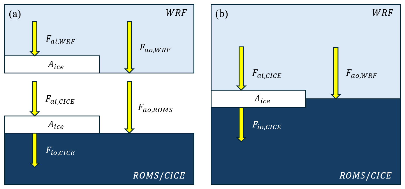
Figure 1 Pathways of surface heat flux exchange between WRF and ROMS/CICE in CAPS for (a) the original coupling approach, and (b) the revised coupling approach.

In this study, we aim to resolve a legacy surface heat-flux inconsistency in CAPS to minimize the inconsistency of heat-flux exchange between the atmosphere and ocean–sea ice components, and to evaluate the revised CAPS comprehensively. Compared with previous regional polar flux-conservation studies, the present work focuses on a pan-Arctic atmosphere–ocean–sea-ice coupling framework, applies the revised coupling over a year-long MOSAiC drift, and evaluates the atmosphere, ocean, and sea-ice components against satellite-derived sea ice products and MOSAiC observations. This paper is structured as follows. Section 2 provides an overview of CAPS focusing on the coupling approach, describes the design of numerical experiments and the model configurations for the model evaluation, and the data measured throughout the MOSAiC campaign. Section 3 presents the evaluation of improved CAPS based on satellite-observed sea-ice conditions and the MOSAiC observations. Concluding remarks and discussions are provided in Sect. 4.

2 Methods and data

2.1 Coupled Arctic prediction system

CAPS consists of the Weather Research and Forecasting Model (WRF version 4.1.2), the Regional Ocean Modeling System (ROMS version 3.8), and the Community Ice CodE (CICE version 6.0.0). The data exchange between WRF and ROMS is achieved by the Model Coupling Toolkit (MCT; Larson et al., 2005). Instead of exchanging data through MCT, CICE is embedded within ROMS as subroutines. The integrated ROMS and CICE use the same model time step to better reflect that temperature and salinity of the surface layer will be instantaneously adjusted under supercooled conditions in ROMS, and the freezing/melting potential is calculated accordingly for CICE to form/melt sea ice (adapted from Smith et al., 2010). The required forcing variables of CICE held by ROMS and the CICE-derived variables to ROMS are exchanged through the ROMS–CICE internal coupler every oceanic/sea-ice time step. All model components of CAPS use the same horizontal model grid so that the data exchange between model components does not involve horizontal interpolation.

2.1.1 Original coupling approach

Turbulent heat fluxes of ice-covered ocean cells in WRF and ROMS are based on the mosaic method:

$$\begin{array}{}\text{(1)}& F=(\mathrm{1}-A_{\text{ice}})\times F_{\text{ao}}+A_{\text{ice}}\times F_{\text{ai}/\text{io}},\end{array}$$

where F is the summed turbulent heat flux for driving the boundary layer physics in WRF or as the vertical boundary conditions in ROMS, F_ao is turbulent heat flux at the atmosphere–ocean interface, $F_{\text{ai}/\text{io}}$ is turbulent heat flux at the atmosphere–ice or the ice–ocean interface, and A_ice is sea-ice concentration. Figure 1 shows the schematic of turbulent heat flux calculation in CAPS. On the ROMS side, F_io is provided by CICE based on a Rossby similarity law (Maykut and McPhee, 1995) and F_ao is based on the Coupled Ocean–Atmosphere Response Experiment (COARE) 3.0 bulk formula (Fairall et al., 2003). On the WRF side, F_ai is computed by the Noah land surface physics (Chen and Dudhia, 2001) and F_ao is calculated by the COARE 3.0 algorithm. However, CICE calculates its own F_ai with a stability-based boundary parameterization (Jordan et al., 1999). Also, WRF and ROMS do not share the same modifications for implementing the COARE 3.0 algorithm. In other words, the heat flux inconsistency exists at the WRF–ROMS/CICE interface in the original CAPS (Fig. 1a).

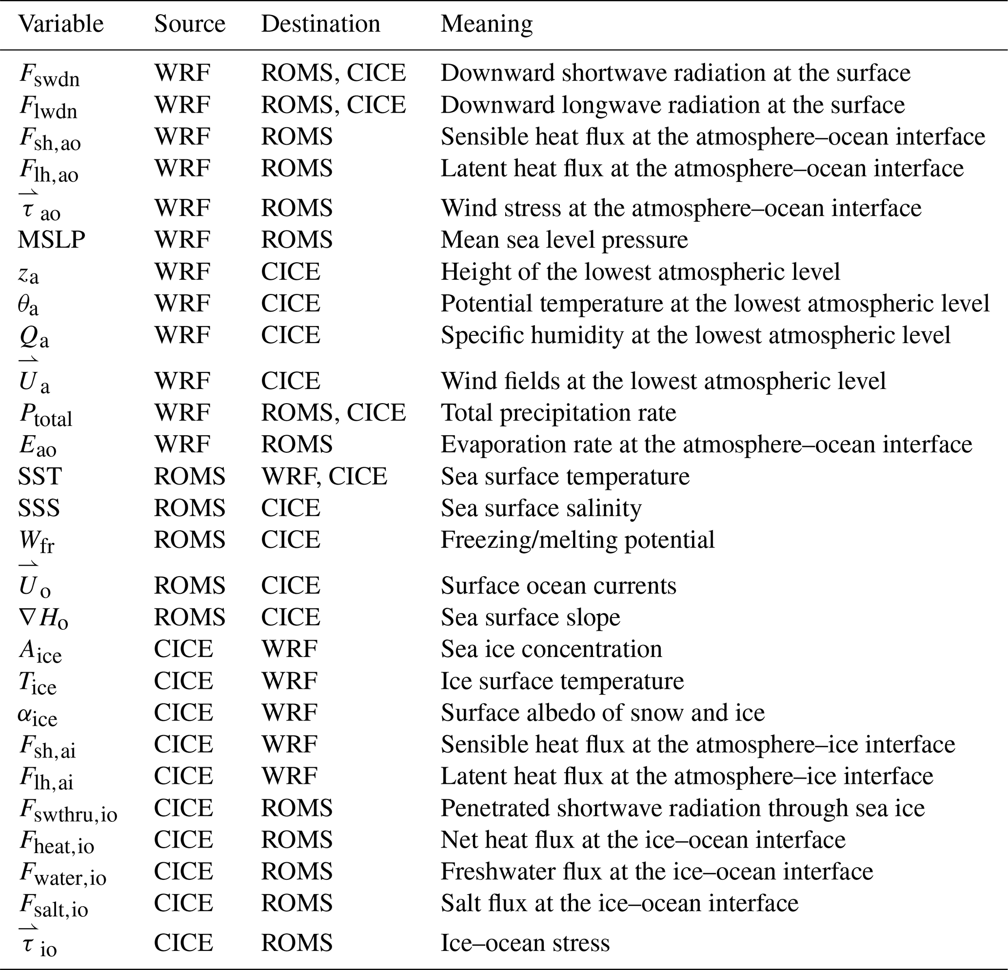
Table 1 List of exchanged variables in CAPS with the revised coupling approach.

2.1.2 Revised coupling approach

To address the inconsistency in turbulent heat flux calculation within CAPS, only one model component is designated to calculate turbulent heat fluxes for all interfaces (Fig. 1b), i.e., turbulent heat flux calculations at the atmosphere–ice and atmosphere–ocean interfaces are revised. Specifically, WRF determines turbulent heat fluxes at the atmosphere–ocean interface based on the COARE 3.0 parameterization for ROMS to receive. Turbulent heat fluxes at the atmosphere–ice interface are calculated in CICE based on wind fields, potential temperature, and specific humidity of the lowest atmospheric level, and the corresponding height from WRF (see Table 1), and CICE-derived heat fluxes are transferred to WRF.

In addition to turbulent heat fluxes, the related variables (i.e., surface temperature, albedo, and emissivity) involved in the radiation physics in WRF also use the same mosaic approach as in Eq. (1) for ice-covered cells. Both WRF and ROMS use 0.06 as the ocean surface albedo. As for the ice surface albedo, the delta-Eddington scheme in CICE determines the absorption of downward shortwave radiation at the ice surface (Briegleb and Light, 2007), which influences the ice surface albedo diagnostic. However, the original ice surface albedo diagnostic based on the delta-Eddington scheme occasionally returns out-of-bound values (i.e., larger than one), and zero ice surface albedo in case of zero downward shortwave radiation (e.g., polar night regions). The following approach is applied in CICE to provide full coverage of ice surface albedo, α_ice, to WRF:

$$\begin{array}{}\text{(2)}& {\mathit{\alpha }}_{\text{ice}}=\left\{\begin{array}{ll}(F_{\text{swdn}}-F_{\text{swabs}})/F_{\text{swdn}}& \text{if }{F}_{\text{swdn}}>\mathrm{0}\\ {\mathit{\alpha }}_{\text{ccsm}}& \text{if }{F}_{\text{swdn}}=\mathrm{0}\end{array}\right.,\end{array}$$

where F_swdn is the downward shortwave radiation from WRF, F_swabs is the ice-absorbed shortwave radiation based on the delta-Eddington scheme, and α_ccsm is the diagnostic albedo based on the parameterization used in the Community Climate System Model, which is the function of snow/ice surface temperature, ice thickness, snow thickness, and the spectrum of downward shortwave radiation. The surface emissivity of ocean, 0.984, is used for both WRF and ROMS (Konda et al., 1994), and WRF uses the same value (0.95) as in CICE for the surface emissivity of snow and ice. Warren (2019) reported that ice surface emissivity is 0.92 and snow surface emissivity is 0.98–0.99. Table 1 summarizes the variables that WRF, ROMS, and CICE exchange through the couplers with the improved coupling approach. The variables exchanged with the original coupling approach are also summarized in Table S1 in the Supplement.

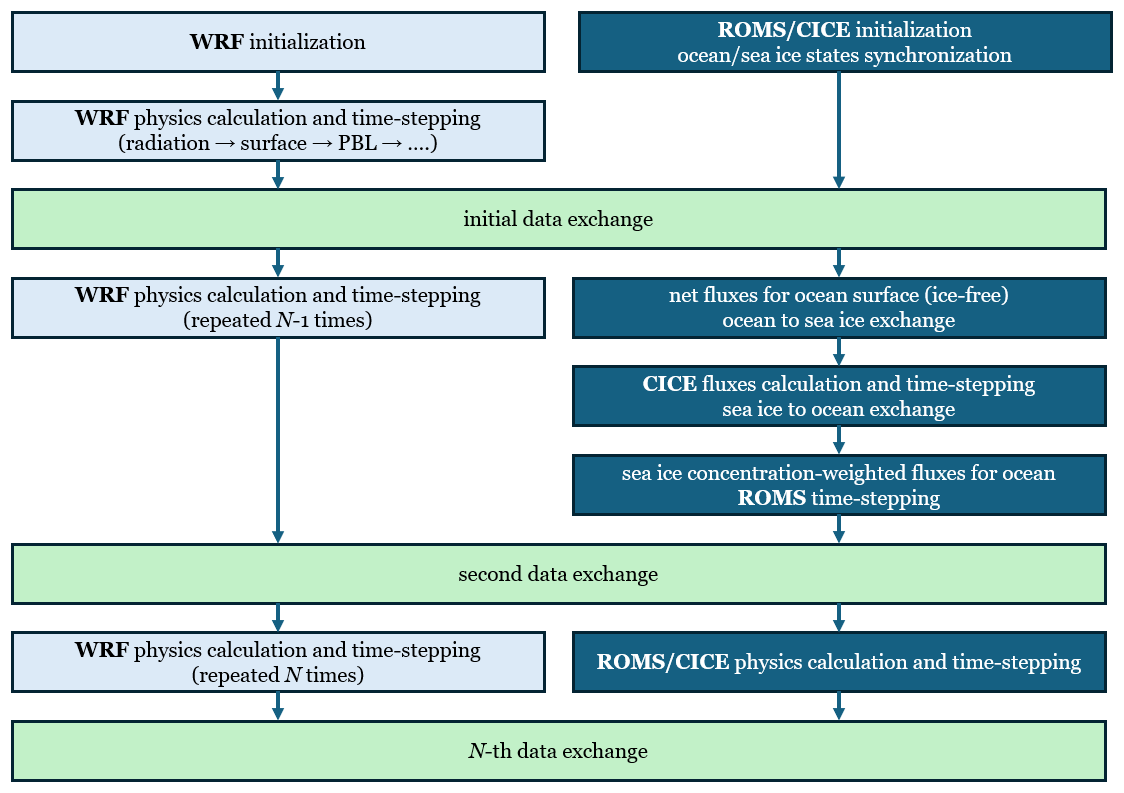
Figure 2 Schematic model sequence diagram for coupling between WRF and ROMS/CICE. The steps taken in WRF and ROMS/CICE are visualized as the light blue and dark blue blocks. The variable exchange is represented as the light green block.

This revised coupling approach is similar in the concept of the flux-conservation approach used in P-SKRIPS (Malyarenko et al., 2023), where fluxes computed by the atmospheric component are imported into the ocean-sea ice component to avoid repeated and inconsistent flux calculations. The implementation in CAPS differs in the flux ownership assigned by interface: WRF is used as the source of atmosphere–ocean turbulent heat fluxes, whereas CICE is used as the source of atmosphere–ice turbulent heat fluxes and transfers these fluxes back to WRF. This design preserves the surface fluxes exchanged between the atmosphere and ocean–sea ice components while retaining the existing WRF–ROMS–CICE coupling structure.

2.1.3 Coupling cycle

The model sequence of each model component in the CAPS based on the revised coupling approach is illustrated in Fig. 2. In our implementation of the revised coupling in CAPS, WRF calculates its physical processes for the first atmospheric time step to determine all variables (see Table 1), before the initial data exchange between WRF and ROMS/CICE, which provides non-zero values for precipitation and downward radiative heat fluxes to drive ROMS/CICE physics until the next data exchange. Originally, the surface layer scheme in WRF updates the values of ice surface (e.g., surface temperature and turbulent heat fluxes). In our implementation, the surface layer scheme still updates the related variables of ice surface to maintain the stability of WRF, but the summed values based on Eq. (1) with the CICE-derived values (turbulent heat fluxes of ice surface, ice surface temperature, and ice surface albedo) are the final output values for the boundary layer scheme and the radiation transfer scheme in WRF.

After receiving values from WRF, ROMS will determine the net heat (net radiative heat fluxes plus turbulent heat fluxes), net salt (evaporation minus precipitation), and momentum fluxes of the ocean surface assuming grid cells are ice-free. Subsequently, CICE receives its required variables (see Table 1) through the ROMS-CICE internal coupler, computes fluxes at the atmosphere–ice and ice–ocean interfaces, and then updates ice state variables to the next sea-ice time step. The computed heat, water, salt, and momentum fluxes at the ice–ocean interface are integrated with the fluxes of ocean surface calculated previously based on Eq. (1) as the final top boundary conditions for ROMS to update its state variables to the next oceanic time step.

Table 2 Summary of physic options and details of the revised CAPS.

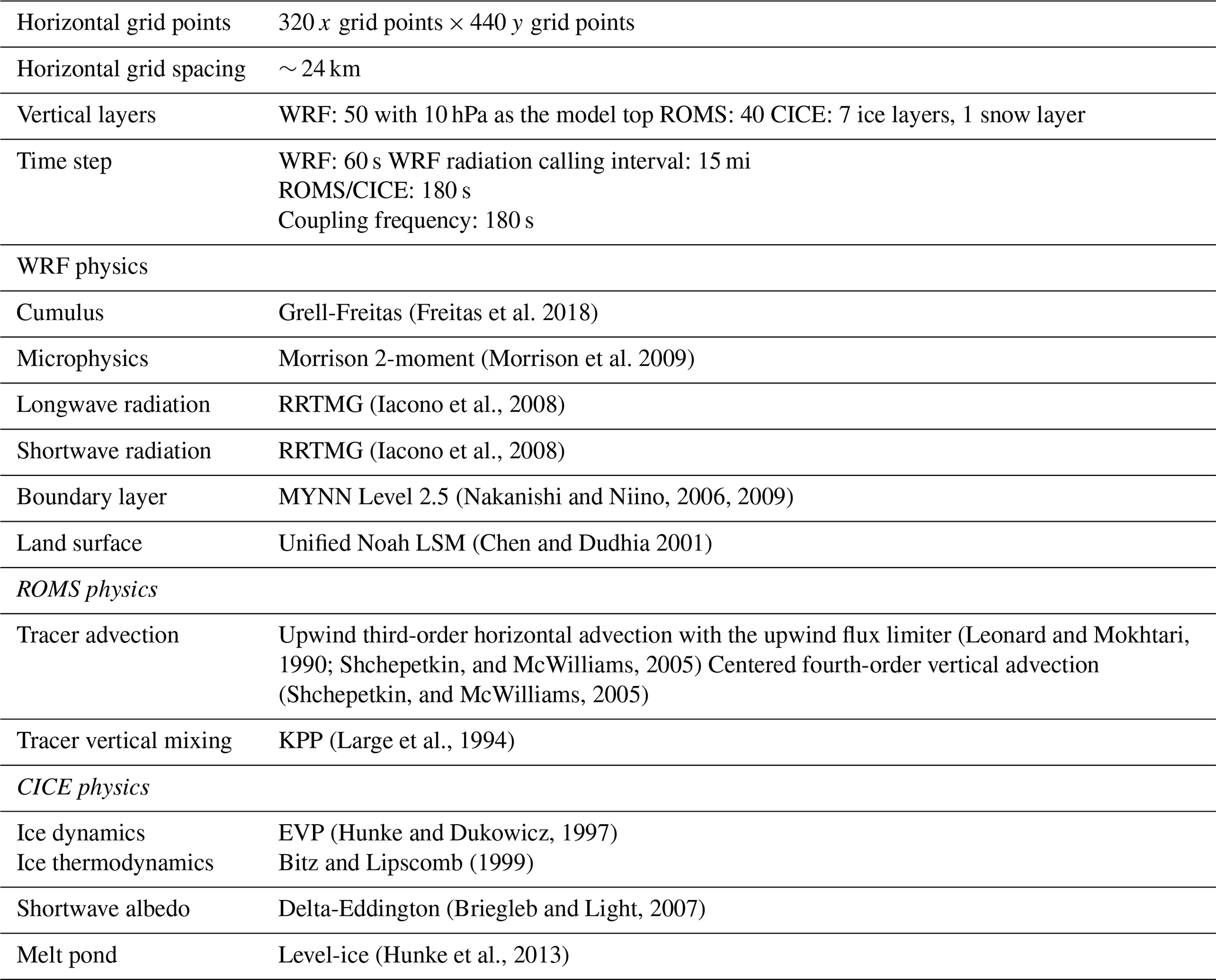
As described in Sect. 2.1, the same horizontal model grid for all model components in CAPS makes WRF demand more computational resources than ROMS/CICE. WRF is also more restrictive in atmospheric time step compared to ROMS. To balance the computational loading between WRF and ROMS/CICE, WRF is configured to integrate more atmospheric time steps before exchanging data with ROMS/CICE in this study, and WRF exchanges data with ROMS/CICE every oceanic/sea-ice time step (Fig. 2, Table 2, and see Sect. 2.2 for the exact setup). Note that all data exchanges are done with instantaneous fields without employing time averaging over a coupling cycle in this study.

2.2 Model configurations and simulation designs

In this study, the model domains of WRF, ROMS, and CICE are the same as the previous pan-Arctic configurations of CAPS (Yang et al., 2022, 2024, and see Fig. S1 in the Supplement). The domain includes 320 x- and 440 y-grid points with ∼ 24 km horizontal resolution on the polar stereographic projection. Initial and lateral boundary conditions for WRF are generated from the fifth generation of European Centre for Medium-Range Weather Forecasts Reanalysis (ERA5, Hersbach et al., 2023, last access: 30 November 2025), with 6-hourly time spacing and a spatial resolution of 0.25°. During the initialization processes of WRF, we specify the initial top of lowest model layer to 10 m, which provides ∼ 5 m for the height of the lowest model layer (z_a, see Table 1), and the remaining model layers (50 layers in total, see Table 2) are determined by the default stretching parameters. Global Ocean Ensemble Physics Reanalysis (GREP) produced by Copernicus Marine Service (https://doi.org/10.48670/moi-00024, last access: 30 November 2025) is utilized to create initial and lateral boundary conditions for ROMS and CICE. The ensemble of GREP includes Global Ocean ReanalYses and Simulations (GLORYS2V4), Ocean Reanalysis System 5 (ORAS5), and the CMCC Global Ocean Reanalysis Systems (C-GLORSv7). GREP provides daily mean oceanic and sea-ice states with a spatial resolution of 0.25°, and the ensemble mean is used for ROMS and CICE. Previous studies have shown that GREP can provide reasonable estimates of sea-ice and oceanic states in the Arctic (Cocetta et al., 2024; Yao et al., 2025).

In this study, three experiments covering the entire period of the MOSAiC expedition, starting from 00:00 UTC 1 September 2019, to 00:00 UTC 1 November 2020 were conducted, and the three primary experiments serve different purposes. Exp_FREE_OLD provides the baseline simulation using the original coupling approach. Exp_FREE uses the revised coupling approach without spectral nudging and is used to evaluate the free-running behavior of the revised CAPS after correcting the heat-flux inconsistency. Exp_NUD uses the revised coupling approach with spectral nudging and is designed as a constrained hindcast experiment in which the large-scale atmospheric state is constrained toward ERA5. The spectral nudging in Exp_NUD is applied to wind, temperature, and humidity, with horizontal wavenumbers 1–3 nudged toward ERA5 data, and only at grid points above the boundary-layer height. The revised coupling approach presented in this study does not guarantee that other physical parameterizations in CAPS are free of biases in polar regions. Previous studies have shown that Arctic weather and climate prediction remains challenging because of limitations in the representation of stable boundary layers, clouds and radiation, atmosphere–ocean–sea-ice exchange, sea-ice/snow processes, and data assimilation under sparse polar observations (e.g., Ortega et al., 2022; Inoue, 2021; Guemas et al., 2016; Vihma, 2014; Hines et al., 2015). Therefore, differences between Exp_FREE_OLD and Exp_FREE primarily reflect the effect of the revised coupling, whereas differences between Exp_FREE and Exp_NUD reflect the sensitivity to the representation of the large-scale atmospheric state. The improved agreement with observations in Exp_NUD should therefore be interpreted as the combined effect of the revised coupled model and the imposed large-scale atmospheric constraint, rather than as an improvement caused by the revised coupling or model physics alone.

Physical options of each model component are mostly identical to those used in Yang et al. (2024) with several differences for the revised CAPS. For shortwave and longwave radiation, the Rapid Radiative Transfer Model (RRTMG, Iacono et al., 2008) is utilized as the radiation transfer scheme in WRF. The vertical tracer mixing scheme in ROMS is changed to the Large–McWilliams–Doney interior closure scheme, also known as K-profile parameterization (KPP, Large et al., 1994) with several compiling options (controlled by C-preprocessor keywords) activated in ROMS including surface boundary layer mixing (LMD_SKPP), bottom boundary layer mixing (LMD_BKPP, Durski et al., 2004), non-local transport (LMD_NONLOCAL), convective mixing due to shear instability (LMD_CONVEC), double-diffusive mixing (LMD_DDMIX), the effect of shear instability on diffusivity (LMD_RIMIX), and Shapiro filter to boundary layer depth (LMD_SHAPIRO, Shapiro 1970). Further details of physics options and experiment configurations are summarized in Table 2.

2.3 Evaluation data

2.3.1 MOSAiC data

To evaluate the performance of the revised CAPS, the observations from the MOSAiC expedition are utilized, which include radiosondes, the MOSAiC cloud observing suite, meteorological tower, atmospheric surface flux stations (ASFS), conductivity-temperature profiling through depth (CTD) buoys, and snow and ice mass balance array (SIMBA) buoys (Nicolaus et al., 2022; Rabe et al., 2022; Shupe et al., 2022). These observations were distributed within the MOSAiC observational network, including the central observatory (CO), three large sites (L1, L2, and L3) located approximately 15 km from CO, and several medium sites (M1–M8) distributed over a broader area. This distribution of the MOSAiC sites is shown in Fig. 2 of Bliss et al. (2023). For atmospheric observations, radiosondes were launched four times per day, typically at 05:00, 11:00, 17:00, and 23:00 UTC during MOSAiC. These radiosondes provide vertical profiles from 12 m up to an altitude of about 30 km for temperature, relative humidity, pressure, and winds (Maturilli et al., 2022). The cloud observing suite includes multiple sensors (e.g., cloud radar, depolarization lidar, microwave radiometer, and ceilometer), which provide time-height derivations of cloud microphysical properties (e.g., the cloud type, the condensed water content) (Shupe, 2022). The meteorological tower at Met City (the CO site) measured surface radiative (both downward and upward) heat fluxes with 1 min average intervals. Turbulent heat fluxes were calculated from the tower measurements based on the eddy covariance method with 10 min average intervals (Cox et al., 2023e). Three ASFS flux measurements, which provide radiative and turbulent fluxes, located at the L1, L2, and L3 sites are also utilized, and these flux measurements will be averaged spatially for the evaluation. For oceanic observations, a set of 8 ice-tethered buoy systems with five CTD units at depths of 10, 20, 50, 75, and 100 m observing temperature and salinity with 2 min intervals are chosen (Hoppmann et al., 2022). Note that only the CTD-buoy at the M1 site, which provides long records of temperature and salinity, is used for the evaluation. For sea-ice observations, SIT and snow depth measured by SIMBA buoys with 6 h intervals are used (Lei et al., 2021). SIT can be highly heterogeneous, ranging from a few centimeters to several meters within ∼ 50 km horizontal distance (e.g., Fig. 2.2 of Haas, 2017). SIT observed by the SIMBA buoys can also be different across each buoy due to the spatial heterogeneity of SIT. Also, the SIMBA buoys were not deployed simultaneously during the MOSAiC expedition, and some buoys only provide relatively short records of SIT and snow depth. SIMBA buoys with relatively long temporal coverage were selected for averaging over their shared period from December 2019 to June 2020. These buoys were located at the CO site (T56, T62, and T66), the L1, L2, and L3 sites (T63, T67 and T70), and the M4 site (T58), which was close to CO. The operational periods of SIMBA buoys during MOSAiC are referred to Fig. 2 of Lei et al. (2022). Daily averages from these measurements will be compared with the grid cell nearest to the observations in the modeled daily mean outputs. The track of the MOSAiC expedition started in the northern Laptev Sea, began to move across the central Arctic with the Transpolar Drift, and finally reached the sea-ice edge in Fram Strait (Fig. 1 of Bliss et al., 2023).

2.3.2 Satellite-derived and reanalysis-based sea-ice data

Since the data collected during the MOSAiC expedition can only provide point observations along the drift, satellite-derived and reanalysis-based sea-ice data are also utilized to evaluate the revised CAPS spatially. For sea-ice concentration (SIC), the daily SIC obtained from the National Snow and Ice Data Center (NSIDC) is chosen in this study. The SIC data is measured by Nimbus-7 Scanning Multichannel Microwave Radiometer (SMMR), the Defense Meteorological Satellite Program (DMSP), Special Sensor Microwave/Imagers (SSM/Is), and Special Sensor Microwave Imager/Sounder (SSMIS) passive microwave sensors, and the SIC data is on the NSIDC polar stereographic grid with a spatial resolution of 25 km (NSIDC_0051, DiGirolamo et al., 2022, last access: 30 November 2025). For sea-ice thickness (SIT), the statistically merged SIT based on CryoSat-2 and Soil Moisture and Ocean Salinity satellite data (CS2SMOS, Ricker et al., 2017, last access: 30 November 2025) is utilized. However, satellite-based SIT is not available during the melting season since satellite cannot distinguish the mixture of wet snow/sea ice, melt ponds, and open water (e.g., Huntemann et al., 2014). The daily SIT produced by the Pan-Arctic Ice Ocean Modeling and Assimilation System (PIOMAS, Zhang and Rothrock, 2003) is chosen to fill the data gap in CS2SMOS.

3 Results

3.1 Evaluation

3.1.1 Evaluation of sea-ice concentration and thickness

In this section, we first evaluate the revised CAPS focused on Exp_FREE and Exp_NUD (with Exp_FREE_OLD as reference) against satellite-based sea-ice observations to provide an overview of the performance of revised CAPS in simulating sea-ice conditions over the pan-Arctic domain during the MOSAiC period. Figure 3 shows the evolutions of SIE of the observations, Exp_FREE, Exp_NUD, and Exp_FREE_OLD, as well as the integrated ice-edge error (IIEE, Goessling et al., 2016) of Exp_FREE, Exp_NUD, and Exp_FREE_OLD with respect to the observations. SIE is computed as the summation of areas of all cells with at least 15 % SIC, and the observed SIE is calculated from NSIDC-0051 SIC. IIEE is defined as the sum of areas where the simulation and the observation disagree on SIC of the same cell being above or below 15 %. The smaller (larger) IIEE indicates that the simulated distribution of sea-ice edges is comparable (different) to the observed distribution. As shown in Fig. 3a, both Exp_FREE and Exp_NUD can reasonably reproduce the seasonal cycle (i.e., the timing of maximum and minimum) of SIE during the MOSAiC period, and both experiments show an underestimation of 1.0 ∼ 1.5 × 10⁶ km² in SIE with respect to the observations around March 2020. In general, the evolution of SIE in Exp_FREE (Fig. 3a) shows smaller SIE for 2019/2020 winter months (November 2019 to April 2020) and larger SIE for 2020 summer months (June to October 2020) compared to that in Exp_NUD (Fig. 3a). As reference, Exp_FREE_OLD (Fig. 3a) simulates larger SIE than Exp_FREE, and the differences in SIE become significantly larger in 2020 summer, indicating the original coupling approach used in the previous version of CAPS (Fig. 1a) may be prone to drifting to a state with extensive sea-ice coverage as the model integrates for a longer period. IIEE of Exp_NUD (Fig. 3b) is generally smaller than that of Exp_FREE (Fig. 3b) for most of the simulation period, suggesting that Exp_NUD shows better performance in simulating the distribution of sea-ice edges than Exp_FREE. Compared with Exp_FREE, Exp_FREE_OLD (Fig. 3b) shows generally smaller IIEE from September 2019 to April 2020 corresponding to better agreement between the simulated SIE in Exp_FREE_OLD and the observed SIE. After July 2020, Exp_FREE_OLD shows generally larger IIEE than Exp_FREE.

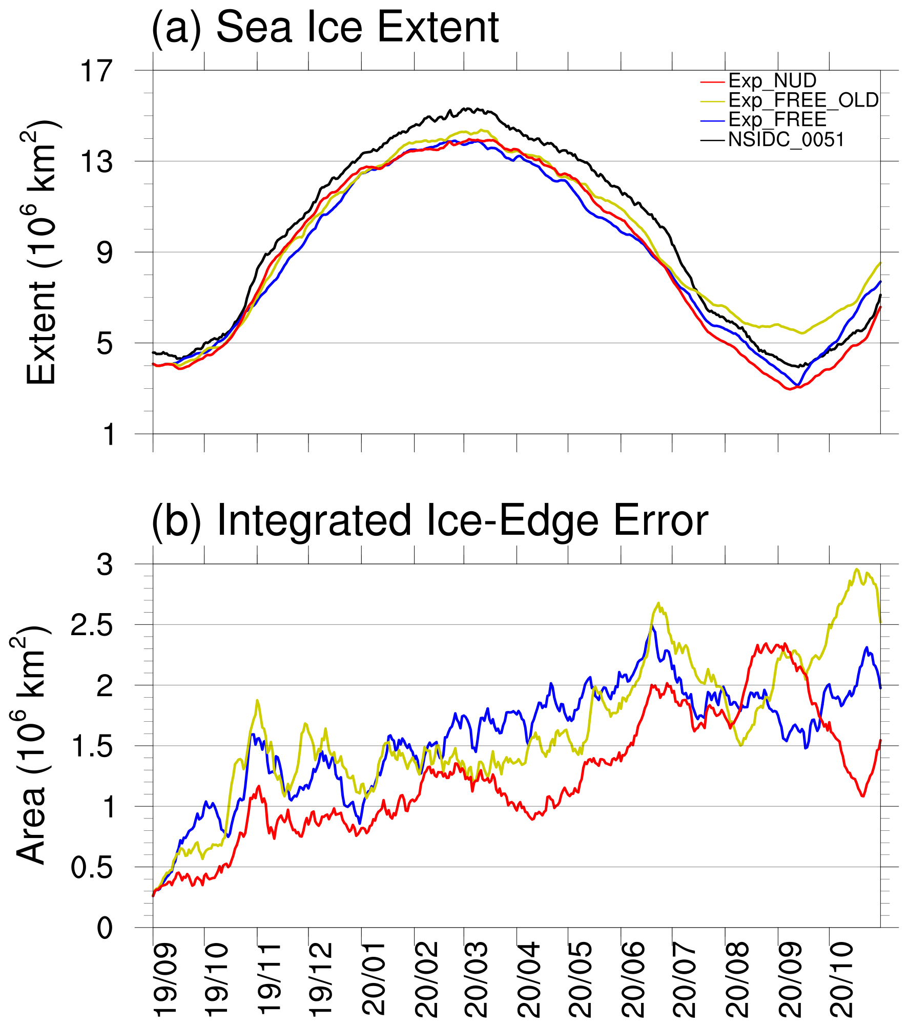
Figure 3 Time-series of (a) Arctic sea ice extent for the observations (NSIDC-0051, black line), Exp_FREE_OLD (yellow line), Exp_FREE (blue line), and Exp_NUD (red line), and (b) integrated ice-edge error for Exp_FREE_OLD, Exp_FREE, and Exp_NUD.

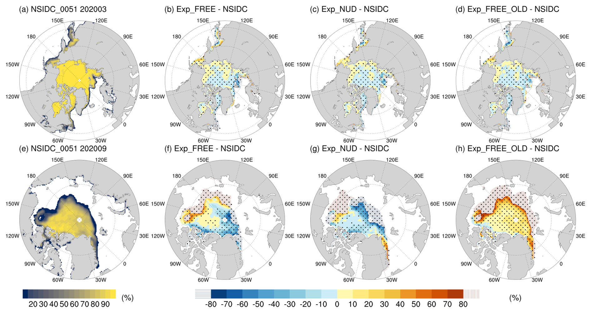
Figure 4 Monthly mean sea ice concentration (SIC) for the observations in (a) March 2020, and (e) September 2020, and the difference between the experiments and the observations for Exp_FREE, Exp_NUD, and Exp_FREE_OLD in (b–d) March 2020, and in (f–h) September 2020. Note: vertical/horizontal-lining represents the overestimated/underestimated local sea ice extent with respect to the observed local sea ice extent, following the definition of IIEE (Goessling et al., 2016); black dotted area denotes grid cells where the mean paired SIC difference is significantly different from zero based on a two-sided paired t-test, after Benjamini–Hochberg false discovery rate correction at q=0.05.

The monthly averaged March and September SIC fields from the observations in 2020, together with the difference between the simulations and the observations, are shown in Fig. 4. Following the IIEE definition of Goessling et al. (2016), the lined areas in Fig. 4b–d and f–h indicate grid cells where the simulated and observed local SIE disagree based on the 15 % SIC threshold. Specifically, underestimated local SIE refers to regions where the observed SIC exceeds 15 % but the simulated SIC does not, whereas overestimated local SIE refers to regions where the simulated SIC exceeds 15 % but the observed SIC does not. Corresponding to the SIE shown in Fig. 3a, the underestimated SIE of Exp_FREE and Exp_NUD in March 2020 mainly arises from underestimated local SIE in the Sea of Okhotsk, the Barents Sea, the Labrador Sea, and Davis Strait (Fig. 4b and c). In contrast to better agreement with the observed SIC shown in Exp_NUD (Fig. 4c, colored areas), Exp_FREE simulates larger SIC in the Bering Sea and smaller ice coverage in the Barents Sea in March 2020 (Fig. 4b). Generally, Exp_FREE_OLD shows larger ice coverage (e.g., in the Sea of Okhotsk, and the Barents Sea) than Exp_FREE in March 2020 (Fig. 4b and d). In September 2020, the areal coverage of overestimated local SIE along the coasts of Alaska, central Siberia, and eastern Siberia was comparable to that of underestimated local SIE near Fram Strait and the Canadian Archipelago. These opposing biases partially offset each other, resulting in a smaller difference in total SIE between Exp_FREE and the observations (Figs. 3a and 4f). In contrast, underestimated local SIE in the central Arctic Ocean and Canadian Archipelago, partly compensated by overestimated local SIE in the Chukchi Sea, is the main contributor to the underestimated SIE in Exp_NUD (Figs. 3a and 4g). Exp_FREE_OLD shows that most of the Arctic Ocean is covered by ice with at least 15 % SIC (Fig. 4h) corresponding to significant overestimation of SIE in summer 2020 shown in Fig. 3a.

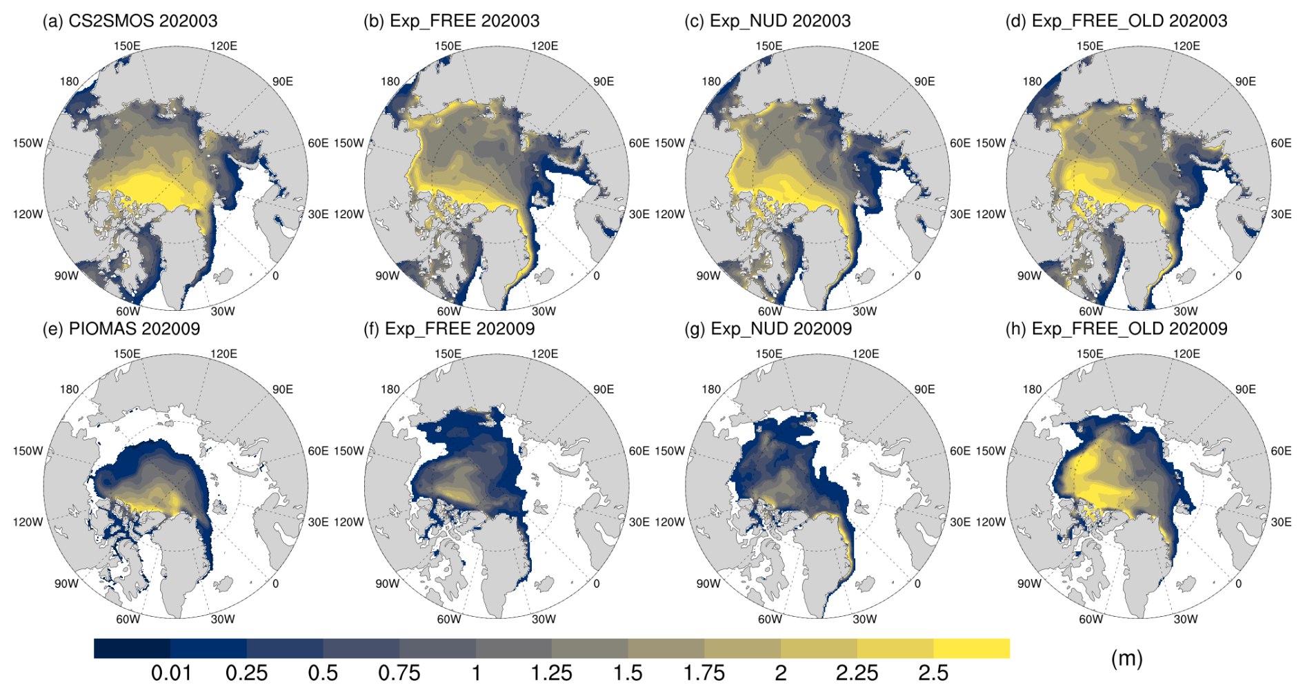
Figure 5 Monthly mean sea ice thickness for the reference data (CS2SMOS and PIOMAS), Exp_FREE, Exp_NUD, and Exp_FREE_OLD in (a-d) March 2020, and (e-h) September 2020.

Figure 5 shows the monthly-averaged March and September SIT of the reference data and the simulations in 2020. The average SIT of all cells with at least 1 % SIC for the reference data and the simulations in March and September 2020 are also shown in Fig. S2. In March 2020, all experiments can reproduce the general patterns of SIT compared with CS2SMOS, showing the thickest ice located north of the Canadian Archipelago with decreasing thickness gradient toward Siberia (Fig. 5a–d). However, all experiments show more areas of thicker sea ice in the Western Arctic Ocean, especially along the coastal areas of Alaska and eastern Siberia. Exp_FREE simulates overall thinner SIT (∼ 1.13 m, Fig. S2) in the Arctic Ocean compared with Exp_NUD (∼ 1.16 m, Fig. S2). For regional difference, Exp_NUD shows thicker SIT in the north of the Canadian Archipelago and Alaska but thinner SIT along the Siberia coast compared to Exp_FREE (Fig. 5b and c). Corresponding to larger ice coverage of Exp_FREE_OLD in March 2020 (Fig. 4d), Exp_FREE_OLD shows relatively thicker SIT (∼ 1.17 m, Fig. S2) in most of the Arctic Ocean than Exp_FREE (Fig. 5b and d). The simulated biases of SIT in September 2020 of both experiments are partly associated with those in March 2020. That is, the thinner SIT along the Siberia coast in Exp_NUD is less persistent, and the thicker SIT along the coastal areas of Alaska and eastern Siberia in Exp_FREE and Exp_NUD in March 2020 is more persistent (Fig. 5b, c and f, g). The overestimated and underestimated local SIE in September 2020 (Fig. 4f andg) are also associated with the simulated bias of SIT in March 2020, such as the OLSIE of Exp_FREE and Exp_NUD in the Chukchi Sea, and the underestimated local SIE of Exp_NUD in the central Arctic Ocean. The evolution of SIT from April 2020 to August 2020 shown in Fig. S3 also illustrates the lasting influence of simulated bias of SIT in March 2020. Generally, Exp_NUD shows better agreement with CS2SMOS and PIOMAS than Exp_FREE in both March and September 2020 (Figs 5 an S2). In Exp_FREE_OLD, most of the Arctic Ocean is still covered by sea ice with the average SIT of 1.25 m in summer 2020 (Figs. 5h and S2), which is significantly thicker than Exp_FREE (∼ 0.54 m, Fig. S2) and Exp_NUD (∼ 0.59 m, Fig. S2), corresponding to extensive ice coverage in most of the Arctic Ocean shown in Fig. 4h.

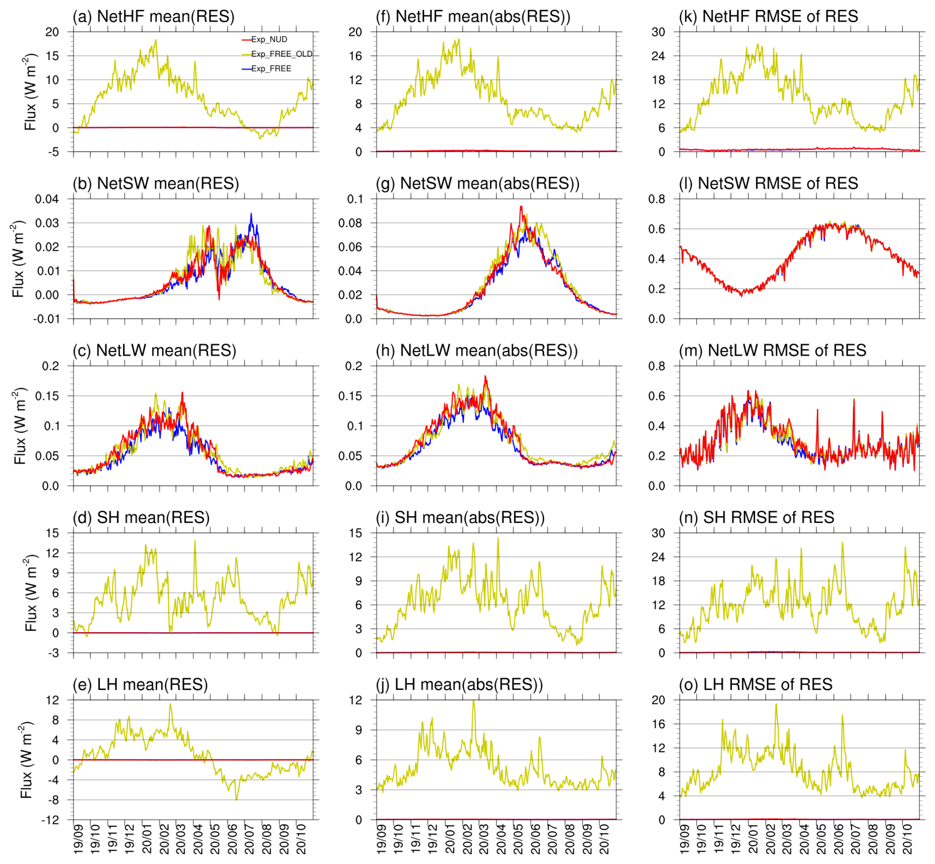
Figure 6 Domain-averaged statistics of interfacial heat-flux residuals at atmosphere–ocean–sea-ice coupling cells for all flux components in Exp_FREE_OLD (yellow line), Exp_FREE (blue line), and Exp_NUD (red line). The statistics include the (a–e) mean residual, (f–j) mean absolute residual, and (k–o) root-mean-square error (RMSE), with residuals defined by Eq. (3).

3.1.2 Evaluation of improved flux coupling

To diagnose the consistency of heat-flux exchange between the atmosphere and the ocean-sea-ice components with the original and revised coupling approaches, we define the residual of interfacial heat-flux exchange at the atmosphere–ocean–sea-ice coupling cells, which can be expressed as

$$\begin{array}{}\text{(3)}& \begin{array}{rl}{R}_{\text{coupling}}(x,y,t)=& F_{\text{surface}}^{\text{WRF}}(x,y,t)\\ & -F_{\text{surface}}^{\text{ROMS}/\text{CICE}}(x,y,t),\end{array}\end{array}$$

where $F_{\text{surface}}^{\text{WRF}}$ is the flux component used in the WRF physical processes, and $F_{\text{surface}}^{\text{ROMS}/\text{CICE}}$ is that in the ROMS/CICE processes. Both $F_{\text{surface}}^{\text{WRF}}$ and $F_{\text{surface}}^{\text{ROMS}/\text{CICE}}$ are the weighted averaged fluxes based on Eq. (1). The flux component is defined as positive downward and includes net surface heat flux (NetHF), with the components of net shortwave radiative flux (NetSW), net longwave radiative flux (NetLW), sensible heat flux (SH), and latent heat flux (LH). Figure 6 shows the domain-mean residual, domain-mean absolute residual, and root-mean-square error (RMSE) of interfacial heat-flux residuals for all flux components in Exp_FREE_OLD, Exp_FREE, and Exp_NUD. Exp_NUD is included in this residual analysis as an additional check that the revised coupling maintains similar interfacial heat-flux residuals under the constrained-atmosphere configuration. Mean residuals of NetHF are 0∼ 15 W m⁻² for most of the simulation period with the original coupling approach (Exp_FREE_OLD), whereas those with the revised coupling approach (Exp_FREE and Exp_NUD) are negligible (less than 0.1 W m⁻², Figs. 6a and S4a). Since all fluxes are defined positive downward, positive (negative) residuals of NetHF represent that the ocean-sea ice component receives less (more) energy than it is supposed to receive, which can be also viewed as an artificial cooling (warming) effect in the ocean-sea ice coupled system due to the inconsistency in heat-flux exchange. Mean residuals of NetHF in Exp_FREE_OLD are mainly contributed by turbulent components rather than radiative components (Fig. 6a–e). Mean residuals of SH are mostly positive throughout the simulation, with the magnitude ranging from ∼ 0 to ∼ 12.5 W m⁻² (Fig. 6c). Mean residuals of LH are mostly positive from September 2019 to April 2020 (up to ∼ 11.5 W m⁻²) and then negative afterward (up to ∼ 8 W m⁻²) (Fig. 6d). For Exp_FREE and Exp_NUD, the mean (Fig. 6a–e), mean absolute (Fig. 6f–j), and RMSE residuals (Fig. 6k–o) remain much smaller than those in Exp_FREE_OLD, confirming that the revised coupling substantially reduces both the systematic and local/intermittent interfacial heat-flux residuals. The remaining residuals are generally small and mainly reflect numerical and diagnostic differences rather than the large systematic inconsistency seen in Exp_FREE_OLD. The contrast between Exp_FREE_OLD and Exp_FREE demonstrates the effect of the revised coupling itself, because both experiments are free-running and differ primarily in the coupling approach. The similarly small residuals in Exp_NUD indicate that the revised coupling remains consistent when spectral nudging is applied.

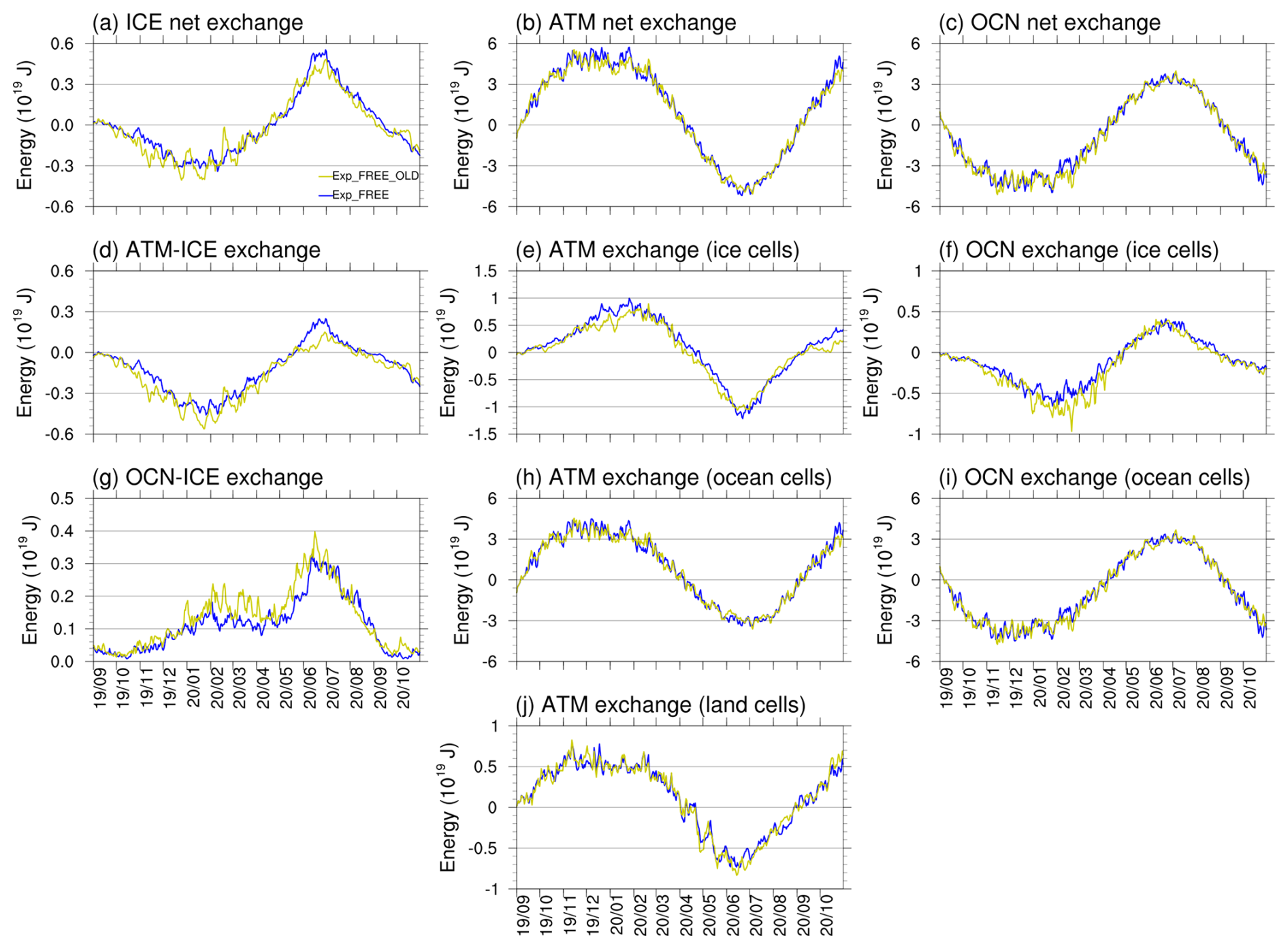
Figure 7 Daily integrated surface/interfacial energy exchange for the (a) sea-ice, (b) atmosphere, and (c) ocean in Exp_FREE_OLD (yellow line) and Exp_FREE (blue line). Sea-ice energy exchange is decomposed into (d) atmosphere–ice and (g) ice–ocean contributions; atmospheric lower-boundary exchange is separated into (e) ice-covered, (h) open-ocean, and (j) land cells; and ocean upper-boundary exchange is separated into (f) ice-covered and (i) open-ocean cells. Note: positive values indicate energy gain by the component or interface named in each panel; ice-covered cells are defined by SIC ≥ 1 %.

To place the interfacial residuals shown in Fig. 6 into a coupled-system energy-cycle context, we further diagnose the daily integrated energy exchange through the lower boundary of the atmosphere, the atmosphere–ice and ice–ocean interfaces of sea ice, and the upper boundary of the ocean for Exp_FREE_OLD and Exp_FREE (Fig. 7). Positive values represent energy gain by the component or interface indicated in each panel. Because the purpose of Fig. 7 is to isolate the effect of the coupling revision on the component-level energy pathways, we compare Exp_FREE_OLD and Exp_FREE only; Exp_NUD is not included in this diagnostic because it additionally differs by the use of spectral nudging. Both experiments reproduce a pronounced seasonal surface energy cycle. The atmosphere gains energy from the surface during the cold season and loses energy during the melt season, while the ocean shows the opposite seasonal behavior, with heat loss in autumn–winter and heat uptake in late spring–summer (Fig. 7b and c). These domain-integrated atmospheric and oceanic exchanges are mainly controlled by open-ocean grid cells, as indicated by the close correspondence between the total atmospheric/oceanic energy terms and their open-ocean contributions (Fig. 7h and i), while the ice-covered and land-cell contributions are smaller in magnitude (Fig. 7e, f, and j).

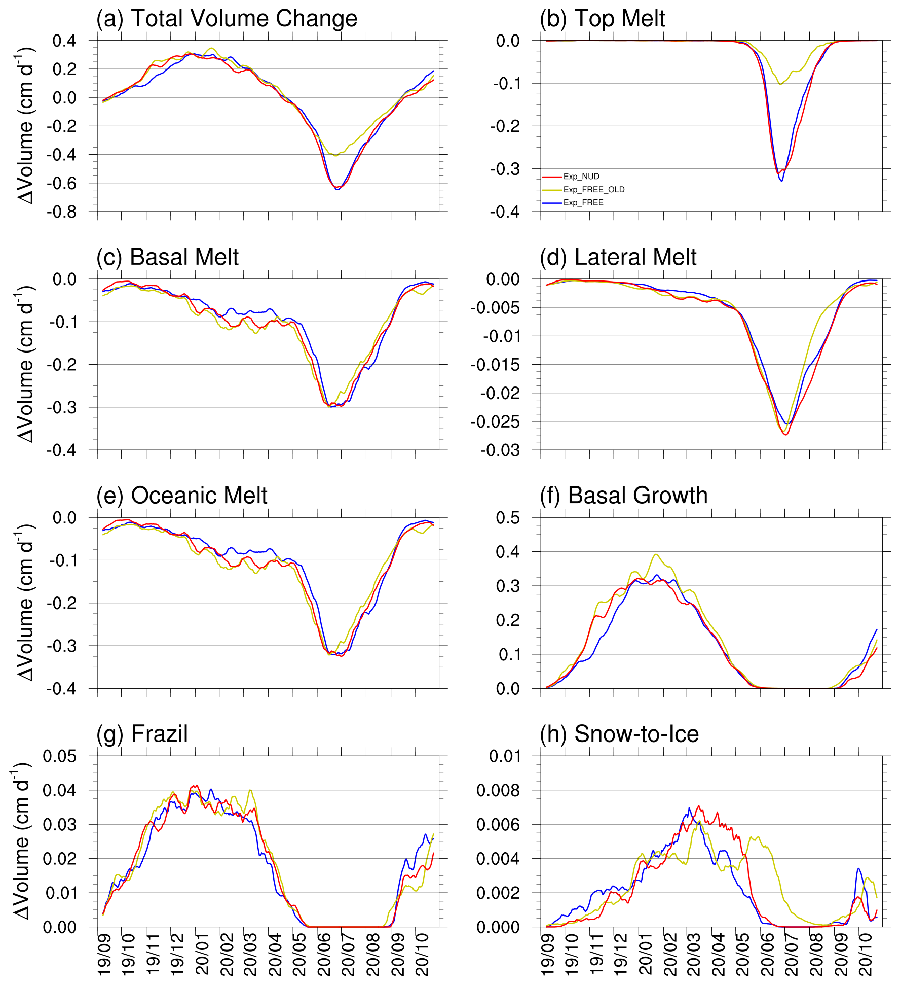
Figure 8 Time-series (15 d running-averaged) of sea ice volume budget for Exp_FREE (blue line), Exp_FREE_OLD (yellow line), and Exp_NUD (red line). Sea ice volume budgets include: (a) total volume change, (b) sea ice melt at the air-ice interface (top melt), (c) sea ice melt at the bottom of the ice (basal melt), (d) sea ice melt at the sides of the ice (lateral melt), (e) sea ice melt from oceanic energy (basal plus lateral melt), (f) sea ice growth at the bottom of the ice (basal growth), (g) sea ice growth by supercooled open water (frazil), and (h) sea ice growth due to transformation of snow to sea ice (snowice). Note: (a)-(h) are averaged over the model domain (Fig. S1).

The sea-ice net exchange is roughly one order of magnitude smaller than the atmospheric and oceanic exchanges but is more directly linked to the simulated sea-ice thermodynamic response. Sea ice loses energy from autumn to early spring and gains energy during the melt season, with a peak in early summer (Fig. 7a). This seasonal transition is mainly controlled by the atmosphere–ice interface: sea ice loses energy to the atmosphere during the cold season and gains energy from the atmosphere during late spring and summer (Fig. 7d). Compared with Exp_FREE, Exp_FREE_OLD generally shows stronger negative atmosphere–ice exchange during winter and weaker positive atmosphere–ice exchange during summer, indicating enhanced cold-season energy loss from sea ice and reduced melt-season atmospheric energy input to sea ice in the original coupling approach. Although differences in the domain-integrated atmospheric and oceanic exchanges are relatively small because they are dominated by open-ocean cells, the differences over ice-covered cells are more evident and directly affect the sea-ice energy pathway. This helps explain why the original coupling approach leads to a cumulative overestimation of sea-ice thickness and coverage during the 14-month simulation, characterized by enhanced winter ice growth and reduced summer ice retreat (Figs. 3–5). This diagnostic represents the surface/interface energy exchange among model components rather than a fully closed three-dimensional prognostic heat budget for each component, because atmospheric and ocean heat storage, lateral boundary transports, and internal source-sink terms are not explicitly included.

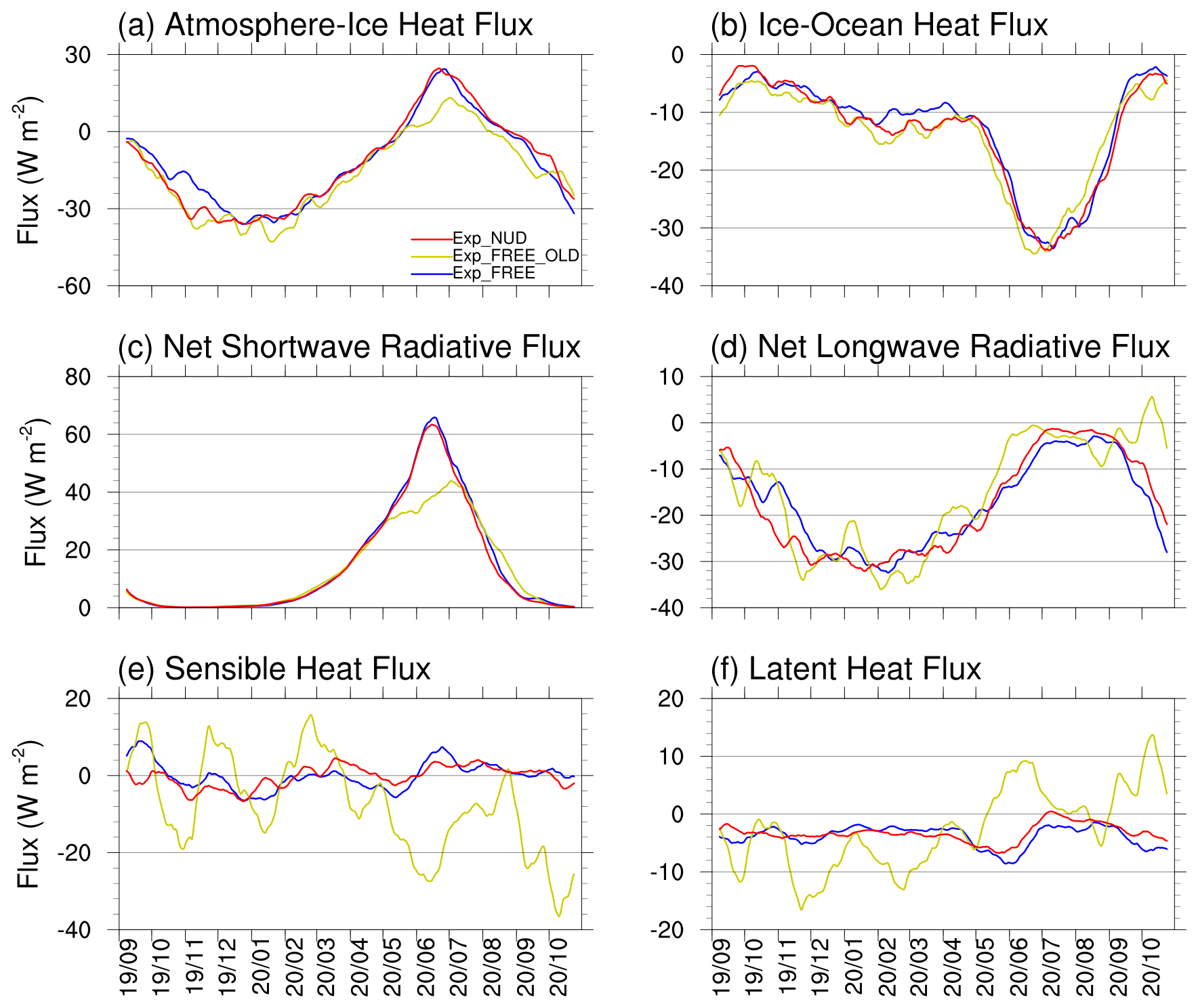
Figure 9 Time-series (15 d running-averaged) of (a) atmosphere–ice heat flux, (b) ice–ocean heat flux, (c) net shortwave radiative flux, (d) net longwave radiative flux, (e) sensible heat flux, and (f) latent heat flux for Exp_FREE (blue line), Exp_FREE_OLD (yellow line), and Exp_NUD (red line). Note: (a–f) are averaged with SIC-weighting over all grid cells with at least 1 % SIC to represent the mean value of the grid cell, and are defined as positive downward.

To further illustrate how the inconsistency in surface heat fluxes degrades the performance of CAPS with the original coupling approach in Exp_FREE_OLD, the evolutions of sea-ice volume (SIV) budget components (with their terminology according to Appendix E of Notz et al., 2016) for Exp_FREE and Exp_FREE_OLD are compared (Fig. 8). Overall, the total SIV tendencies in Exp_FREE_OLD (Fig. 8a) are higher than those in Exp_FREE (Fig. 8a) for most of the simulation, with largest differences (up to 0.2 cm d⁻¹) between both experiments in July 2020 compared to the rest of the simulation. The higher total SIV tendencies in Exp_FREE_OLD indicates that the simulated SIT in Exp_FREE_OLD will become thicker than that in Exp_FREE as the model integrates, which is also shown in the average SIT in March and September 2020 (Fig. S2). The thicker SIT contributes slower retreating of sea-ice coverage during the melting season in Exp_FREE_OLD, corresponding to significantly overestimated SIE shown in Fig. 3a. Compared to Exp_FREE, Exp_FREE_OLD shows higher SIV growth rate at the bottom of the ice (basal growth, Fig. 8f) and from supercooled open water (frazil, Fig. 8g) in 2019/2020 winter and spring, and significantly less SIV melting at the atmosphere–ice interface (top melt, Fig. 8b) in summer 2020.

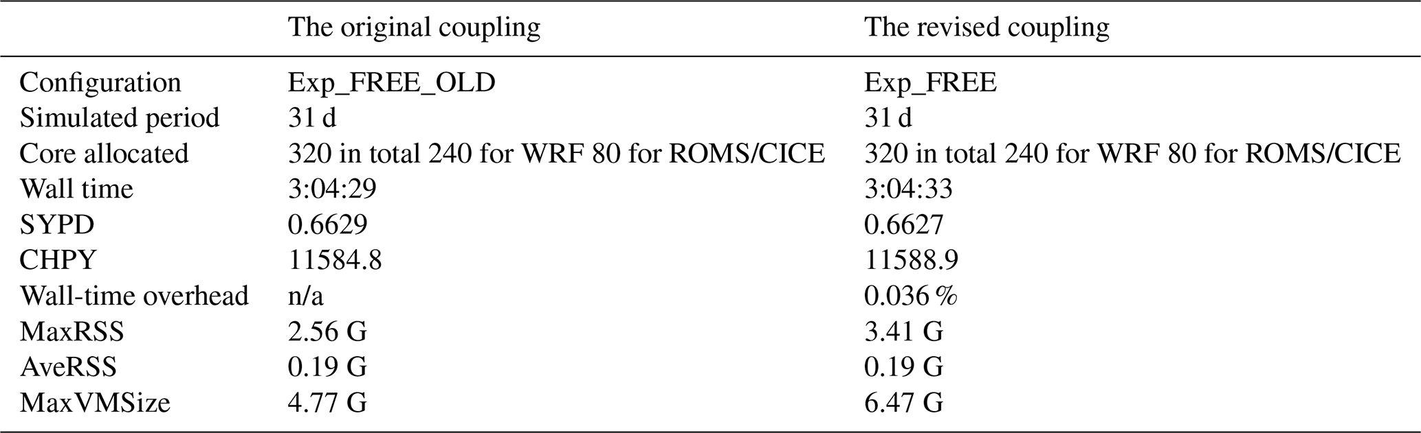
Table 3 Computational-cost benchmark for the original and revised CAPS coupling configurations on an HPC system with two 32-core Intel Xeon Platinum 8358P processors at 2.60 GHz and 512 GB RAM per node. SYPD: simulated years per wall-clock day. CHPY: Core-hours per simulated year. MaxRSS: the maximum resident set size. AveRSS: the average resident set size. MaxVMSize: the maximum virtual memory size.

n/a stands for not applicable, as the wall-time overhead is not defined for the benchmark case.

Figure 9 shows the heat flux budget components at the atmosphere–ice interface and the ice–ocean interface for both Exp_FREE and Exp_FREE_OLD. Generally, the net heat flux at the atmosphere–ice interface (Fig. 9a) is well correlated to the total SIV tendencies shown in Fig. 8a. Larger negative net heat fluxes (i.e., sea ice loses energy to the atmosphere) contribute to larger SIV growth. Accordingly, the larger negative heat flux in Exp_FREE_OLD compared to Exp_FREE drives the larger SIV growth in Exp_FREE_OLD in winter, particularly in January 2020. And, the smaller positive net heat fluxes (i.e., sea ice gains energy from the atmosphere) in Exp_FREE_OLD, compared to Exp_FREE, in July 2020 are responsible for the smaller SIV melting in Exp_FREE_OLD. The decomposition of the net heat fluxes at the ice surface to radiative and turbulent components (Fig. 9c–f) shows that the larger negative net heat fluxes from October 2019 to December 2019 in Exp_FREE_OLD are caused by the combination of latent heat flux and net longwave radiation loss at the surface (which are partially cancelled by oscillated positive sensible heat fluxes). The smaller positive net heat fluxes in Exp_FREE_OLD in July 2020 are mainly dominated by smaller net shortwave radiative fluxes. In contrast to net heat fluxes at the atmosphere–ice interface, net heat fluxes at the ice–ocean interface do not show clear contributions to SIV tendencies in Exp_FREE_OLD (Figs. 8 and 9b).

3.1.3 Computational cost estimation

To document the computational cost of the revised coupling, we conducted 31 d benchmark simulations using the original and revised coupling approaches. Both simulations were integrated from 00:00 UTC 1 October 2019 to 00:00 UTC 1 November 2019 using identical input/output settings, the same node list, and the same processor layout. Wall time and memory usage were obtained from the SLURM accounting record for the model execution step. The throughput shown in Table 3 is reported as simulated years per wall-clock day (SYPD), calculated as

$$\begin{array}{}\text{(4)}& \text{SYPD}={\displaystyle \frac{D_{\text{sim}}/\mathrm{365}}{T_{\text{wall}}/\mathrm{24}}}\end{array}$$

where D_sim is the number of simulated days and T_wall is the wall time in hours. The computational cost is also reported as core-hours per simulated year (CHPY),

$$\begin{array}{}\text{(5)}& \text{CHPY}=T_{\text{wall}}\times N_{\text{core}}\times {\displaystyle \frac{\mathrm{365}}{D_{\text{sim}}}}\end{array}$$

where N_core is the number of allocated cores.

The revised coupling introduces negligible additional wall-clock cost relative to the original coupling. The wall time increases from 3 h 04 min 29 s to 3 h 04 min 33 s, corresponding to an overhead of 0.036 %. The throughput remains nearly unchanged, from 0.6629 to 0.6627 SYPD. The estimated computational cost also changes slightly, from 11584.8 to 11588.9 CHPY. These results indicate that the revised heat-flux exchange does not impose a meaningful computational burden under the benchmarked configuration. The present benchmark should be interpreted as a production-configuration overhead estimation rather than a comprehensive scaling test. The current CAPS domain has a moderate horizontal grid size of 320 × 440, and the production layout already uses 320 cores. For this problem size, further speed-up is expected to be increasingly limited by communication, load balance, and input/output overhead. Because the revised coupling only changes the ownership and exchange of surface-flux variables and does not introduce additional horizontal interpolation, remapping, or new model components, the negligible overhead shown in Table 3 suggests that the revised heat-flux exchange does not materially affect computational performance under the configuration used in this study. A more complete scalability assessment for larger or higher-resolution CAPS configurations is left for future work.

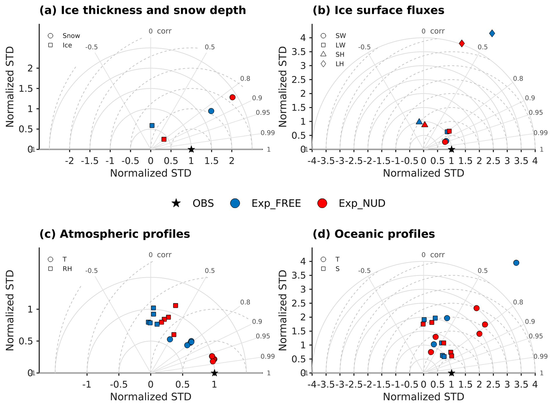
Figure 10 Taylor diagrams comparing simulated and observed (a) ice thickness and snow depth, (b) ice surface heat fluxes, (c) atmospheric profiles, and (d) ocean profiles. Atmospheric variables are evaluated at 1, 3, 5, 7, 9 km using radiosonde observations, oceanic variables at 10, 20, 50, 75, 100 m using CTD observations, and single-level sea-ice and surface variables using their corresponding observation levels. Statistics are calculated from paired model and observation samples for Exp_FREE (blue) and Exp_NUD (red). The Taylor diagrams summarize the correlation coefficient, normalized standard deviation, and normalized centered RMSE, while the corresponding bias and full RMSE are listed in Tables 4 and 5.

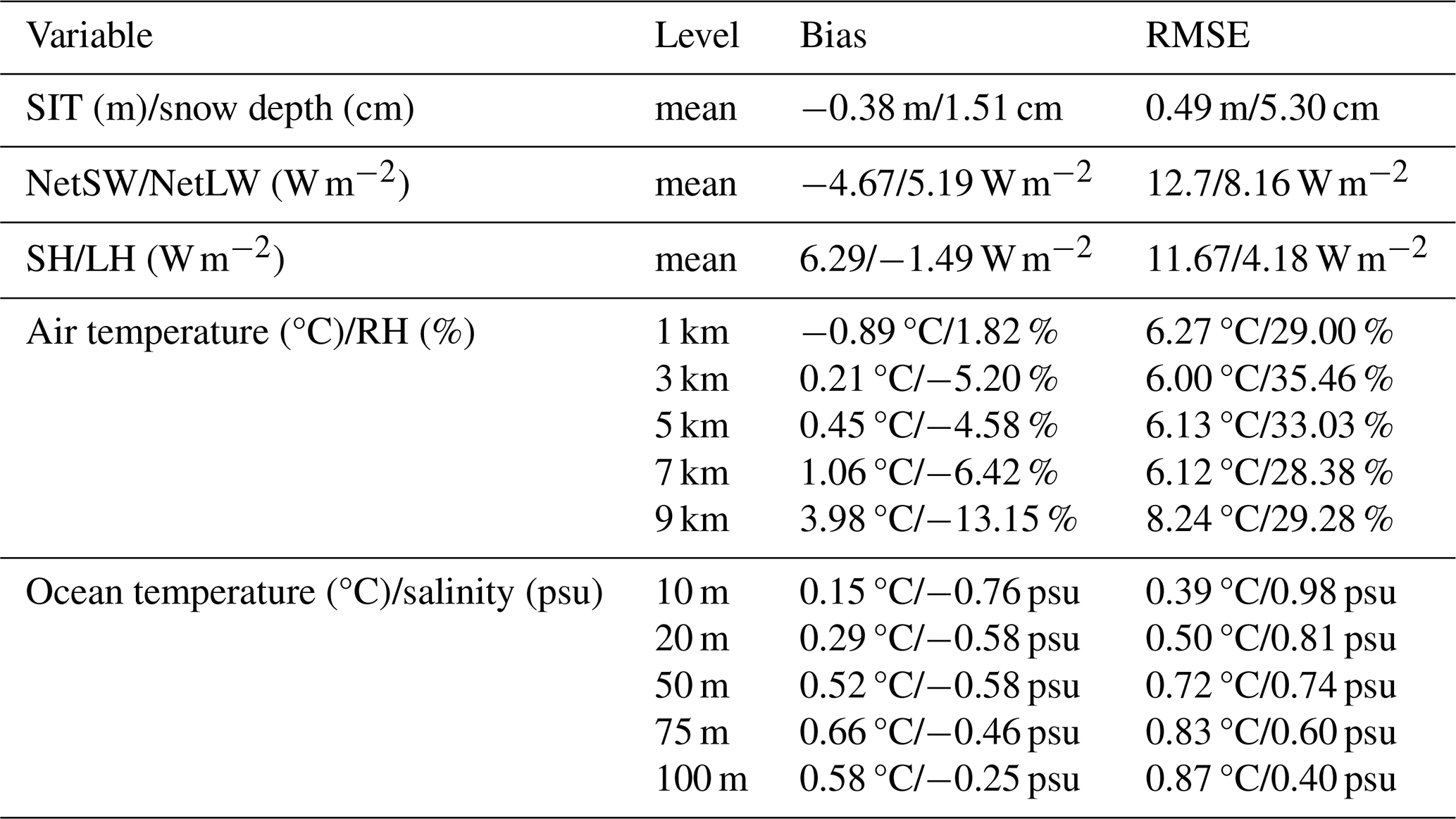
Table 4 Bias and RMSE of Exp_FREE against MOSAiC observations for atmospheric, oceanic, and sea-ice variables. Atmospheric profile variables are evaluated at altitudes of 1, 3, 5, 7, and 9 km, oceanic profile variables at depths of 10, 20, 50, 75, and 100 m, and single-level variables at their corresponding observations levels.

Table 5 Same as Table 4, but for Exp_NUD.

3.2 Evaluation based on the MOSAiC observations

To provide a quantitative evaluation of CAPS against the MOSAiC observations, Fig. 10 summarizes the correlation coefficient, normalized standard deviation, and normalized centered RMSE using Taylor diagrams, while Tables 4 and 5 list the corresponding bias and RMSE of Exp_FREE and Exp_NUD. Atmospheric variables are evaluated at altitudes of 1, 3, 5, 7, 9 km based on radiosonde observations, oceanic variables are evaluated at depths of 10, 20, 50, 75, 100 m based on CTD observations, and single-level sea-ice and surface-flux variables are evaluated at their corresponding observation levels. These quantitative metrics are discussed together with the time-series and profile comparisons in the following subsections.

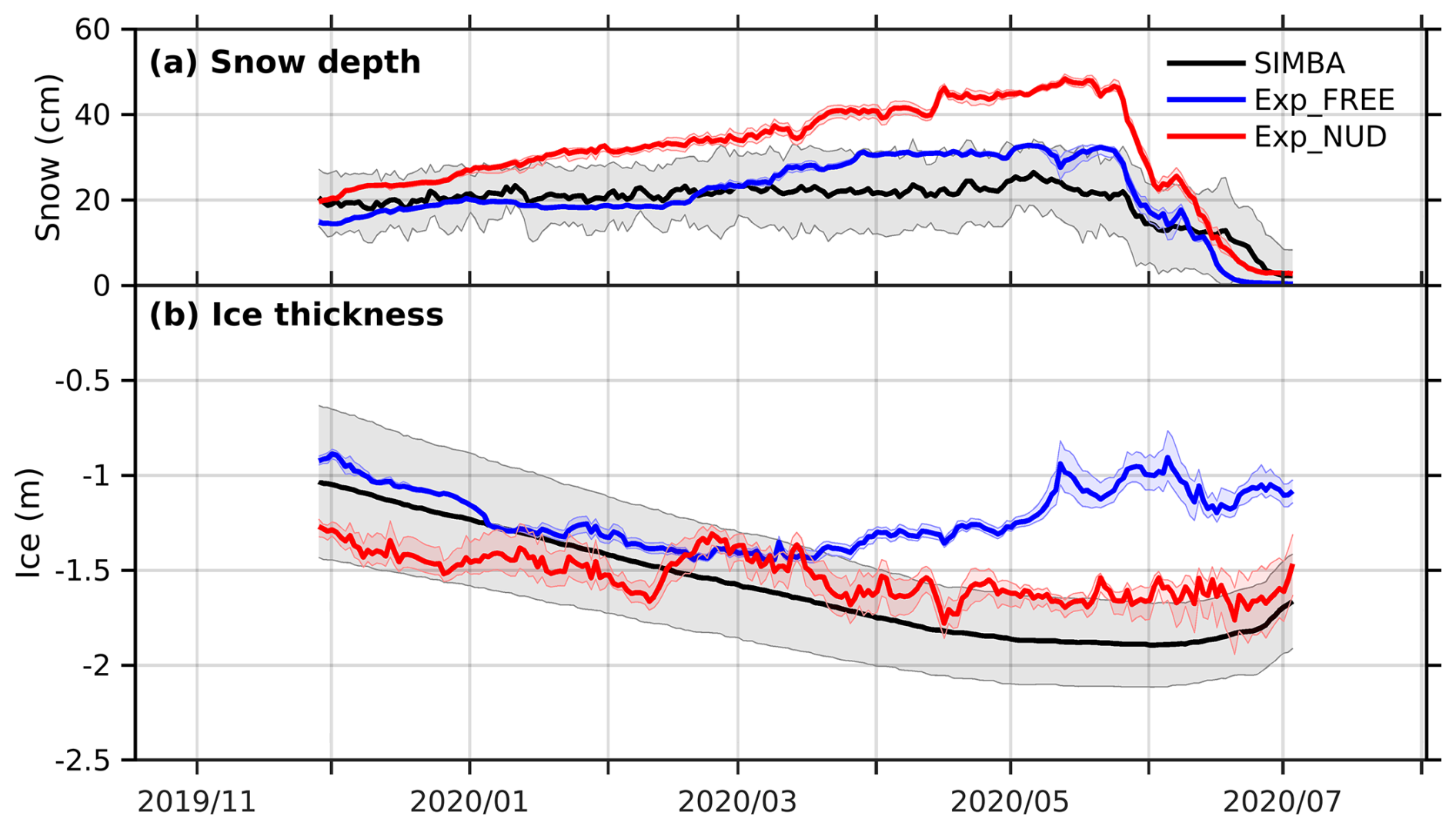
Figure 11 Time-series of daily-mean (a) snow depth and (b) sea ice thickness for SIMBA buoys (black line), Exp_FREE (blue line), and Exp_NUD (red line) along the track of MOSAiC drift. Note: the shadings represent the uncertainty range of the simulated and observed variables. For SIMBA buoys, the uncertainty range is ± 1 standard deviation. For the simulations, the uncertainty range is the range of the nearest grid cell to the observed latitude/longitude and four nearby grid cells.

3.2.1 Snow and ice mass balance

The evolutions of SIT and snow depth for the observations and the simulations along the MOSAiC drift are shown in Fig. 11. For SIT (Fig. 11b), SIMBA shows ∼ 1.0 m ice thickness at the beginning of December 2019 and reaches ∼ 1.9 m at the beginning of June 2020. The simulated SIT of Exp_FREE and Exp_NUD shows some disagreement with that of the SIMBA buoys, which is partly associated with that the simulations do not reproduce exactly the same ice trajectory as the track of SIMBA buoys. Exp_FREE shows similar SIT as the SIMBA buoys at the beginning of December 2019 and comparable thickening changes from December 2019 to February 2020. Afterwards, SIT in Exp_FREE shows early thinning changes relative to the SIMBA buoys. On the other hand, SIT in Exp_NUD shows overall thickening evolutions, which are relatively similar to those by the SIMBA buoys. Exp_NUD also shows thicker SIT compared to the SIMBA buoys (∼ 1.2 m vs. ∼ 1.0 m, which still lies within the uncertainty range of SIMBA) at the beginning of December 2019. For snow depth (Fig. 11a), snow depth observed by the SIMBA buoys is near constant (∼ 20 cm) from December 2019 to June 2020 and then decreases afterward. Both Exp_FREE and Exp_NUD can simulate the timing of snow depth decreases. However, in contrast to the nearly constant snow depth observed from December 2019 to May 2020, both experiments show a continuous increase in snow depth during this period. Also, Exp_NUD shows relatively larger snow accumulation than Exp_FREE. The quantitative metrics are consistent with these features. For SIT, Exp_NUD shows a much higher correlation with SIMBA than Exp_FREE and reduces the bias/RMSE from −0.38 m/0.49 m in Exp_FREE to −0.05 m/0.20 m in Exp_NUD (Tables 4 and 5). In contrast, both experiments show comparable correlations for snow depth, but the normalized standard deviation is larger than one, especially in Exp_NUD, indicating excessive snow-depth variability associated with the simulated snow accumulation events (11a).

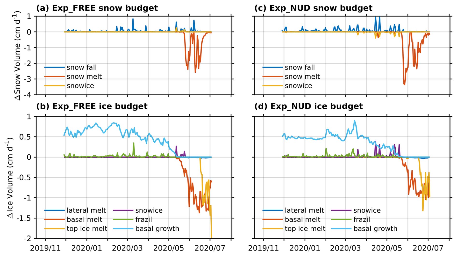
Figure 12 Time-series of snow and sea ice volume budget for (a, b) Exp_FREE, and (c, d) Exp_NUD along the track of the SIMBA buoys.

Similar to SIV budget averaged for the entire domain discussed in Sect. 3.1, the snow and SIV budgets along the track of SIMBA buoys for Exp_FREE and Exp_NUD are shown in Fig. 12 to interpret the above-described simulated biases. Figure 12 indicates that the evolutions of SIT (Fig. 11b), especially the SIT thinning, are primarily driven by basal melt for both Exp_FREE and Exp_NUD. Exp_FREE shows larger basal melt and earlier increases in basal melt than Exp_NUD (Fig. 12b and d). For snow depth, the increase in snow depth in Exp_FREE and Exp_NUD are associated with individual snowing events (i.e., spikes in snow fall shown in Fig. 12a and c). Since snow volume budgets in Exp_FREE and Exp_NUD are well correlated with the evolutions of snow depth shown in Fig. 11a, this indicates that the discrepancy between the simulated snow depth and the SIMBA observations may be associated with missing processes in the CICE model. Currently, ice thermodynamics in the CICE model (Bitz and Lipscomb, 1999; Turner and Hunke, 2015) treat snow and ice as an integral, and snow is not independently transported to other grid cells by surface wind.

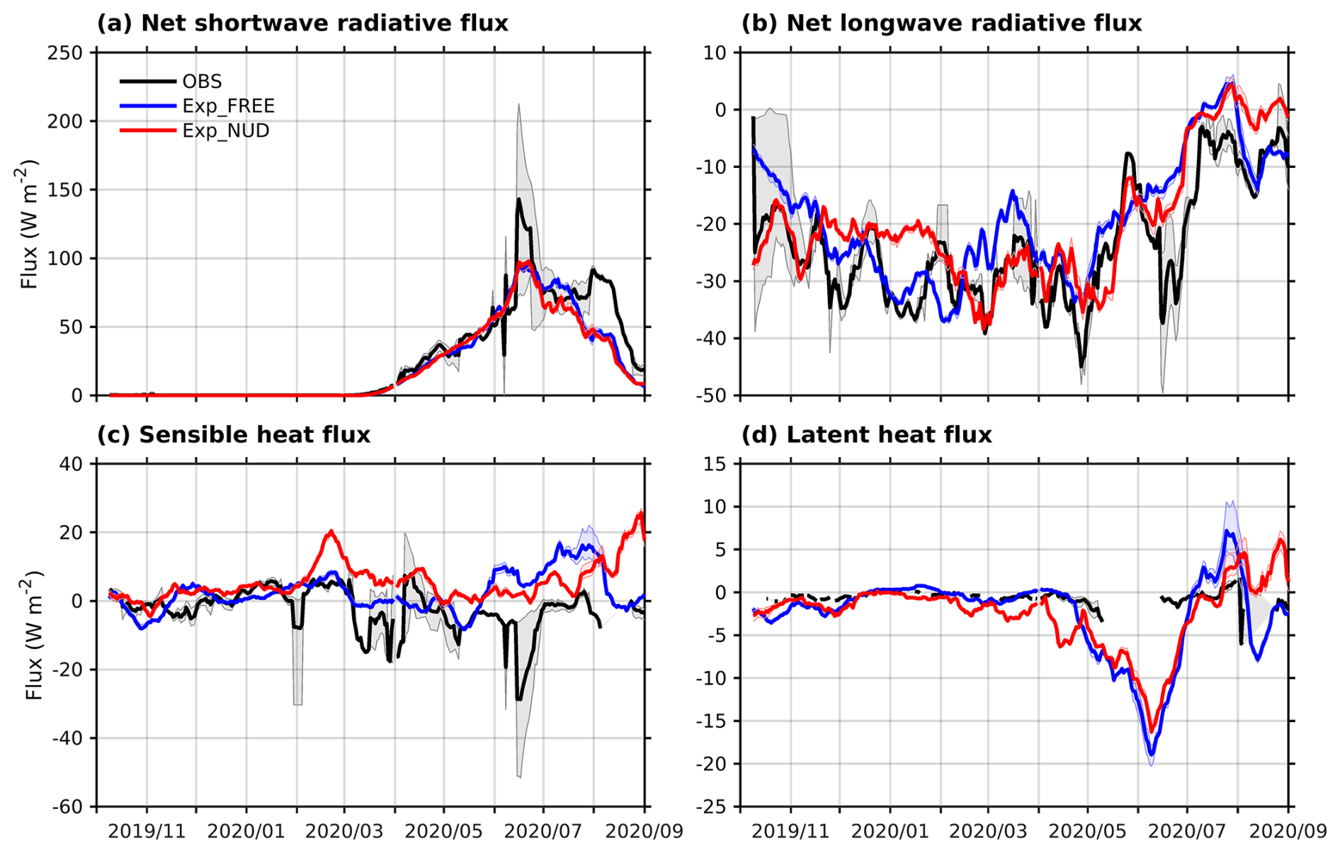
Figure 13 Time-series (15 d running-averaged) of (a) net shortwave radiative flux, (b) net longwave radiative flux, (c) sensible heat flux, and (d) latent heat flux for the observations (black line), Exp_FREE (blue line), and Exp_NUD (red line) along the track of MOSAiC drift. Note: all fluxes are defined as positive downwards. The shadings represent the uncertainty range of the simulated and observed variables. For the observations, the uncertainty range is the range of available sites with non-missing values. For the simulations, the uncertainty range is the range of the nearest grid cell to the observed latitude/longitude and four nearby grid cells.

3.2.2 Surface atmospheric energy budget

Figure 13 shows radiative and turbulent heat fluxes at the ice surface for the observations and the simulations along the MOSAiC drift. For NetSW (Fig. 13a), Exp_FREE, Exp_NUD, and the observations show similar evolution of NetSW from March to June 2020. Afterward, both Exp_FREE and Exp_NUD simulate a smaller peak of NetSW in mid-June 2020 with underestimations of ∼ 40 W m⁻²for both Exp_FREE and Exp_NUD compared with the observations. For NetLW (Fig. 13b), Exp_FREE and Exp_NUD, show different periods with smaller biases compared with the observations from November 2019 to June 2020. Afterward, both Exp_FREE and Exp_NUD show overestimations (∼ 15–25 W m⁻² for Exp_FREE, ∼ 10–15 W m⁻² for Exp_NUD) of NetLW compared to the observed values. For turbulent heat fluxes (Fig. 13c and d), both Exp_FREE and Exp_NUD show similar evolution of SH and LH, and the simulated SH and LH are similar to the observations from November 2019 to February 2020. Afterward, the simulated SH and LH begin to show biases compared with the observed SH and LH, especially the simulated LH from May 2020 to June 2020. Both Exp_FREE and Exp_NUD show different timings with smaller/larger biases in NetLW, SH, and LH compared to the observed values, indicating the grid cell nearest to the locations of the observations in Exp_FREE and Exp_NUD are experiencing different synoptic systems in the atmosphere during the simulation period. The Taylor metrics further show that the radiative fluxes are better constrained than the turbulent fluxes. NetSW and NetLW have relatively high correlations with the observations in both experiments, whereas SH shows weak correlation and LH shows strongly overestimated normalized standard deviation (Fig. 10b). The bias and RMSE statistics indicate comparable overall surface-flux performance between Exp_FREE and Exp_NUD, with Exp_NUD slightly reducing RMSE for NetLW and LH but increasing RMSE for NetSW and SH (Tables 4 and 5). Therefore, spectral nudging applied above the boundary-layer height does not lead to a uniform improvement in all ice-surface flux components along the MOSAiC drift. Although Exp_FREE and Exp_NUD show biases in net radiative and turbulent heat fluxes, the net heat fluxes over the ice surface, which is the major factor determining changes in ice temperature, ice melt, and ice growth in CICE, show better agreement with the observational values for both Exp_FREE and Exp_NUD due to bias cancellation (Fig. S5).

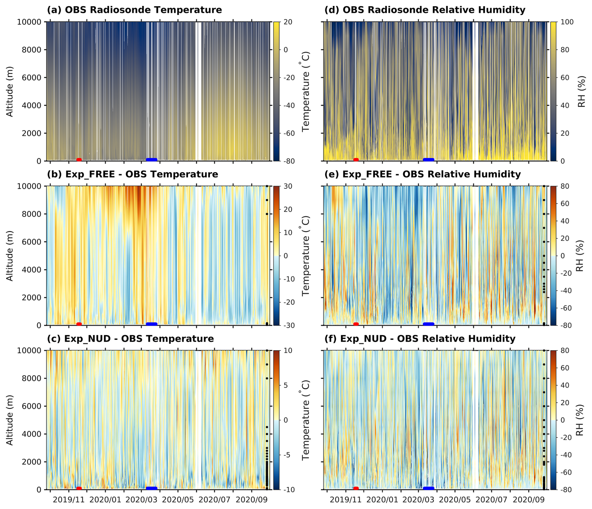
Figure 14 Time-height distributions of radiosonde observations for (a) temperature and (d) relative humidity (RH), the corresponding simulated temperature biases for (b) Exp_FREE, and (c) Exp_NUD, and the RH biases for (e) Exp_FREE, and (f) Exp_NUD along the track of MOSAiC drift. Note: red and blue lines on time-axis represent the STORM-1 and STORM-2 periods; black dots near the right edge of panels (b), (c), (e), and (f) indicate altitude levels where the full-period mean bias is significantly different from zero based on a pair moving-block bootstrap with 3 d blocks and Benjamini-Hochberg false discovery rate correction at q=0.05. The horizontal position of the black dots is for visualization only and does not correspond to a specific time.

3.2.3 Atmospheric profile

Figure 14 shows the vertical profiles of atmosphere temperature and relative humidity (RH) measured by radiosondes launched during the MOSAiC expedition, and the difference between the observations and the experiments along the track of MOSAiC drift. For atmospheric temperature profiles, Exp_FREE simulates profiles with biases oscillating between warm and cold, and the magnitude of biases is larger from October 2019 to April 2020 (Fig. 14b) compared to the rest of periods. From December 2019 to April 2020, Exp_FREE shows excessively warm biases, exceeding 10 °C above ∼ 8 km altitude. In contrast to Exp_FREE, Exp_NUD shows smaller temperature differences relative to the radiosonde observations, with most differences confined within approximately ± 10 °C (Fig. 14c). However, the remaining non-zero differences indicate that constraining the simulated atmosphere toward ERA5 does not eliminate all biases against the MOSAiC radiosondes. These residual differences suggest that the radiosonde comparison is also influenced by uncertainties in the large-scale atmospheric state used for nudging and by sub-grid-scale processes not fully constrained by spectral nudging. Low-level temperature inversions are common features over Arctic sea ice (e.g., Serreze et al., 1992; Devasthale et al., 2010). The inversion structures in the radiosonde observations and all experiments are evaluated in Fig. S6. Exp_FREE reproduces the frequent occurrence of low-level temperature inversions during the cold season, but differs from the radiosondes in their timing and vertical distribution (Figs. S6a and c). With spectral nudging applied, Exp_NUD shows a closer overall representation than Exp_FREE, but still does not fully capture the observed inversion evolution (Figs. S6d). In addition, Exp_FREE_OLD shows stronger inversions during the cold season compared with Exp_FREE, indicating that the inconsistency in heat-flux exchange induced by the original coupling approach (Fig. 6) alters the low-level temperature structure (Fig. S6b).

For RH profiles, Exp_FREE simulates mainly drier profiles with intermittent wetter profiles relative to the radiosondes (Fig. 14e). These intermittent profiles are mainly wetter above ∼ 500 m altitude. Below ∼ 500 m altitude, these intermittent profiles are generally drier compared to the radiosondes. Exp_NUD shows similar patterns in RH profiles (i.e., generally drier, and intermittently wetter above ∼ 500 m altitude) as Exp_FREE, but smaller differences relative to the observations (Fig. 14f). The quantitative metrics confirm that the nudged experiment is closer to the radiosonde profiles than Exp_FREE. For temperature, Exp_NUD shows higher correlations and smaller RMSEs than Exp_FREE at the evaluated altitude levels, and its normalized standard deviations are generally closer to the observations (Fig. 10c; Tables 4 and 5). RH remains more challenging in both experiments, although Exp_NUD also reduces the RMSE of RH relative to Exp_FREE. However, because Exp_NUD constrains the atmospheric state through spectral nudging, these improvements should be interpreted primarily as reduced large-scale atmospheric and synoptic biases, rather than as an isolated improvement of the model physical parameterizations.

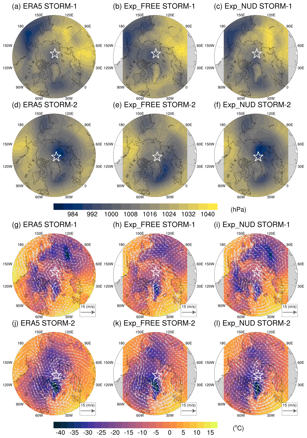
Figure 15 The averaged mean sea level pressure of (a, d) ERA5, (b, e) Exp_FREE, and (c, f) Exp_NUD, and the averaged 2 m temperature and 10 m wind fields of (g, j) ERA5, (h, k) Exp_FREE, and (i, l) Exp_NUD during the period of STORM-1 and STORM-2. Note: white star represents the averaged location of radiosondes during the corresponding storm period, and white gap in panels of simulated fields represents out of model domain (Fig. S1).

The differences in temperature and RH profiles between Exp_FREE and Exp_NUD shown in Fig. 14 are partly associated with the simulated synoptic systems compared with the observations. MOSAiC was characterized by anomalous high frequencies of storms relative to the period of 1979–2020 impacting the trajectory of MOSAiC drift (Liang et al., 2025). These storm events were associated with anomalous meteorological conditions during the MOSAiC period such as anomalously warm conditions by storms during 16 to 20 November 2019, and anomalously low sea level pressure condition by storms during 11 to 25 March 2020 (hereafter referred to as STORM-1 and STORM-2; Rinke et al., 2021). The average mean sea level pressure (MSLP), near-surface air temperature (T2), and 10 m wind fields (UV10) in ERA5, Exp_FREE, and Exp_NUD for the period of STORM-1 and STORM-2 are shown in Fig. 15. The average temperature and RH profiles for Exp_FREE, Exp_NUD, and the radiosondes are also shown in the Supplement (Fig. S7) during both storm periods. During the STORM-1 period, in ERA5, the averaged location of radiosondes (Fig. 15, white stars) is positioned in the central Arctic encompassed by a low-pressure system (Fig. 15a). Exp_FREE also simulates a low-pressure system with lower MSLP encompassing the averaged location of radiosondes (Fig. 15b). The similarity of atmospheric circulations between ERA5 and Exp_FREE near the averaged location of radiosondes results in similar average temperature profiles from surface to 7 km altitude (Fig. S7). During the STORM-2 period, a low-pressure system located over the Barents-Kara Seas encompasses the radiosondes in ERA5 (Fig. 15d) while Exp_FREE shows a low-pressure system centered over the Greenland Sea and the averaged location of radiosondes is positioned at the location with higher MSLP (Fig. 15e). The atmospheric circulations and temperature fields in Exp_FREE result in the warm advection from the North Atlantic to the location of MOSAiC during the STORM-2 period (Fig. 15k), which partly contributes to the warmer profiles in Exp_FREE from surface to ∼ 7 km altitude (Figs. 15 and S7b). Exp_FREE also shows enhanced warm biases above ∼ 7 km altitude for both STORM-1 and STORM-2 periods (Fig. S7a and b). The temperature and wind fields at 8 to 10 km altitude (Fig. S8) show that the warm bias in Exp_FREE increases with altitude. This may be associated with biases from the stratosphere and the model top boundary as suggested by Cassano et al. (2011). In contrast to Exp_FREE, the simulated atmospheric circulations and temperature fields in Exp_NUD resemble those in ERA5 during both storm periods (Fig. 15) corresponding to small temperature biases shown in the simulated profiles (Figs. 14c and S7a–b). However, CAPS with the nudging scheme still faces challenges in simulating RH conditions during the STORM-1 and STORM-2 periods (Fig. S7c and d). As shown by Figs. 14 and 15, the accuracy in simulating the synoptic conditions is crucial for CAPS reproducing the observed vertical thermal structure in the Arctic. The results show that larger biases in Exp_FREE from December 2019 to April 2020 described above (Fig. 14) are partly associated with that Exp_FREE does not properly reproduce these synoptic systems during this period. Liang et al. (2025) also show that the storm events impacting the MOSAiC site are mostly concentrated in the ice growth period (November 2019 to March 2020).

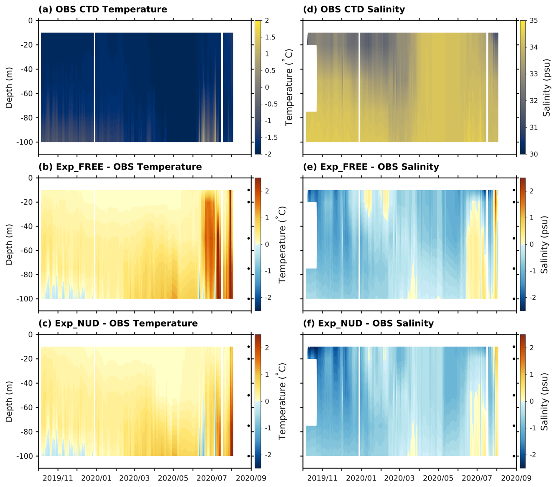
Figure 16 Time-depth distributions of CTD observations for (a) temperature and (d) salinity, the corresponding simulated temperature biases for (b) Exp_FREE, and (c) Exp_NUD, and the salinity biases for (e) Exp_FREE, and (f) Exp_NUD along the track of MOSAiC drift. Note: black dots near the right edge of panels (b), (c), (e), and (f) indicate depth levels where the full-period mean bias is significantly different from zero based on a pair moving-block bootstrap with 3 d blocks and Benjamini-Hochberg false discovery rate correction at q=0.05. The horizontal position of the black dots is for visualization only and does not correspond to a specific time.

3.2.4 Oceanic profile

Figure 16 shows the time-depth distributions of ocean temperature and salinity from the CTD observations, and the corresponding differences between the simulations and observations along the MOSAiC drift. For ocean temperature, both Exp_FREE and Exp_NUD reproduce the overall cold upper-ocean conditions during most of the MOSAiC period, but they show warm biases at different depths and periods (Fig. 16b and c). Before February 2020, both experiments show slightly warmer temperatures by about 0.2–0.4 °C between 30 and 80 m. From March to June 2020, the positive temperature differences increase with depth, and the simulations are about 0.5–1.0 °C warmer than the observations in the 60–100 m layer. Both experiments also show slightly colder temperatures between 80 and 100 m before January 2020. The quantitative metrics indicate that Exp_NUD reduces the ocean-temperature differences relative to Exp_FREE. At evaluated depths of 10, 20, 50, 75, and 100 m, the temperature RMSE decreases from 0.37–0.87 °C in Exp_FREE to 0.17–0.73 °C in Exp_NUD (Tables 4 and 5). The Taylor diagram also shows that Exp_NUD generally has higher correlations and smaller normalized centered RMSEs than Exp_FREE for ocean temperature, especially in the upper 50 m (Fig. 10d). Therefore, the improvement associated with the nudged atmospheric state is more evident for ocean temperature than for salinity.

For salinity, both experiments show fresher upper-ocean biases before December 2019, with differences of about 1.0–2.0 psu in the upper layer (Fig. 16e and f). Afterward, both experiments show better agreement with the observed salinity, with differences generally within ± 0.25 psu in the upper 40 m, and this better agreement extends downward to 100 m until May 2020. However, the quantitative metrics indicate that the salinity improvement is not systematic. Although Exp_NUD shows higher correlations at several depths and slightly smaller normalized centered RMSEs below 20 m, it also shows stronger fresh biases and slightly larger full RMSEs than Exp_FREE at the evaluated depths (Tables 4 and 5). Thus, the salinity biases appear less sensitive to the atmospheric nudging than the temperature biases along the MOSAiC drift.

After June 2020, the significant differences in oceanic temperature and salinity between the simulations and observations are associated with the simulated SIC and upper-ocean thermal structure along the track of CTD buoys. Both Exp_FREE and Exp_NUD show warm biases around July 2020 in the 10–100 m layer, and warm biases in Exp_FREE, exceeding 1.5 °C, are larger than those in Exp_NUD, which are around 0.5 °C. These warm biases correspond to simulated SIC values below 0.9, while the observations still indicate nearly complete ice cover (Fig. S9). The spatial distribution of temperature and salinity at 10, 50, and 100 m depth on 1 July 2020 further indicates that these biases are associated with simulated Atlantic inflow structure (Fig. S10).

4 Conclusions and discussions

This study introduces an improved version of the Coupled Arctic Prediction System (CAPS) that conserves surface heat fluxes between the atmosphere and ocean–sea ice components. A set of pan-Arctic numerical experiments covering the entire MOSAiC expedition was conducted to assess the improvement in simulating Arctic sea-ice conditions contributed by the improved coupling approach, and for the comprehensive evaluation of improved CAPS in simulating the Arctic atmosphere–sea-ice–ocean coupled system against the MOSAiC observations.

Figure 17 Time-height distributions of (a, c) liquid water content, and (b, d) ice water content for the observations and the model simulations during the STORM-1 period.

The results show that the inconsistency in heat-flux exchange between the atmosphere and ocean-sea ice components shown in the previous version of CAPS has been significantly minimized with the improved coupling approach, and the simulated Arctic sea-ice conditions with the improved CAPS are more comparable to satellite-based sea-ice observations than those with the previous version of CAPS. In this study, the simulated sea-ice conditions in the free-running experiment are sensitive to the choices of physics options across the atmospheric, sea-ice, and ocean model components. Simulations conducted with the improved CAPS choosing the same physics options used in the previous version of CAPS (e.g., Yang et al., 2022) can result in the underperformance of the simulated sea-ice conditions (not shown). This indicates further investigations of physical processes in CAPS are required to improve the performance of CAPS. Firstly, CAPS faces challenges in simulating surface heat flux budget over the ice surface. Liu et al. (2024) found that the atmospheric boundary layer observed during MOSAiC can be categorized into a surface inversion type and an elevated inversion type, and the enhanced non-local effects associated with a surface inversion type pose difficulties on similarity theory-based parametrizations to simulate surface sensible heat fluxes. Secondly, CAPS does not reproduce the temperature inversions well compared with the radiosonde observations. The strong temperature inversions in the wintertime Arctic have important effects on the magnitude of downward longwave radiation near the surface (Bintanja et al., 2011). The simulated downward longwave radiation is shown to be associated with the boundary layer stability (e.g., Jozef et al., 2024). Thirdly, surface radiative heat fluxes are regulated by clouds (e.g., Curry et al., 1996; Shupe and Intrieri, 2004). However, it is still challenging for CAPS to properly reproduce liquid water content (LWC) and ice water content (IWC) associated with the frequent occurrence of Arctic mixed-phase clouds and their associated radiative impacts (e.g., Tan et al., 2023) during the MOSAiC expedition. Here, an additional experiment is conducted for the STORM-1 period with high-frequency outputs for cloud properties, and the calculated LWC and IWC compared with the MOSAiC observations are shown in Fig. 17. Generally, CAPS strongly underestimates both LWC and IWC during the STORM-1 period in terms of the occurrence and vertical distribution, which corresponds to the simulated drier atmospheric profiles (Fig. 14). The underestimations of LWC and IWC are associated with the treatment in the microphysics and atmospheric boundary layer schemes (e.g., Arteaga et al., 2024; Sedlar et al., 2020). Arteaga et al. (2024) also suggest that increases in the cloud condensation nuclei and droplet number concentrations in the microphysics schemes can have impacts on the simulated LWC and IWC. Furthermore, it is essential to increase model resolution both horizontally and vertically to properly simulate the phase heterogeneity in Arctic clouds (e.g., Dammann et al., 2025), which demands more computational resources for high-resolution simulations. Regardless of the challenges posed to CAPS, the consistent energy exchange between the atmosphere and ocean–sea ice components in CAPS provides a solid foundation for future improvements in the representation of physical processes, especially for processes related to surface heat flux calculations.

The improved coupling reduces the interfacial heat-flux residuals and improves the simulated sea-ice evolution relative to the original coupling approach in the free-running configuration. In addition to this coupling-focused comparison, the MOSAiC evaluation shows that the constrained-atmosphere experiment, Exp_NUD, agrees more closely with observations in several quantitative metrics, especially for radiosonde temperature/RH profiles and ocean temperature. However, this improved agreement reflects the combined effect of the revised coupled model and the imposed large-scale atmospheric constraint. Moreover, non-negligible biases remain in Exp_NUD, indicating that spectral nudging can reduce errors associated with large-scale atmospheric evolution but cannot fully compensate for biases in physical parameterizations, coupled surface exchange, or the reanalysis fields used for nudging. Therefore, Exp_NUD is used as a sensitivity experiment to examine how the coupled system responds when large-scale atmospheric state is constrained, rather than as evidence that the revised coupling or model physics alone removes the remaining biases.

Because Exp_NUD applies spectral nudging above the boundary-layer height, it represents a relatively strongly constrained experiment. To assess whether the MOSAiC evaluation depends on the vertical extent and strength of this constraint, we conducted two additional sensitivity experiments. Exp_NUD_UPD applies spectral nudging only to the upper 25 of the 50 WRF model levels (approximately above 6.7 km altitude), with a 10-level transition zone from zero to the full nudging weight of 0.0003 s⁻¹, following a design similar to Cassano et al. (2011), whereas Exp_NUD_UPW uses the same vertical design but reduces the nudging weight by one order of magnitude (Glisan et al., 2013). The additional nudging experiments further indicate that the MOSAiC evaluation remains sensitive to the nudging configuration. In the radiosonde comparison, Exp_NUD_UPD and Exp_NUD_UPW both reduce the large temperature departures seen in the free-running atmosphere, but residual temperature and RH differences remain throughout the troposphere, especially in the lower atmosphere and during late summer (Fig. S11). The snow/sea-ice comparison also shows that changing the vertical extent and strength of nudging modifies snow accumulation and melt timing, while the simulated SIT remains within the broad observational uncertainty (Fig. S12). Surface fluxes are likewise sensitive to the nudging setup, in particular turbulent heat fluxes during spring and summer (Fig. S13).

In this study, the implementation of our revised coupling approach is based on the shared horizontal grid between the atmosphere component and the ocean-sea ice component. For applications that require higher resolution (e.g., sea-ice linear kinematic features, ocean eddies in polar oceans), both the atmosphere model and the ocean-sea ice model have to increase their resolutions to the same grid in our current coupling approach, which may be computationally unrealistic for the atmosphere component. CAPS does have the capability to use different grids for the atmosphere component and the ocean-sea ice component through the interpolation weightings generated by the Earth System Modeling Framework (ESMF). However, the interpolation is performed on a mask-to-mask basis in CAPS, i.e., a smaller ocean-sea ice grid cell may represent a larger ocean mask (especially near the complex topography) in the atmosphere component. That is, the spatial heterogeneity of the surface types (i.e., the mixture of land, ocean, and sea ice) within a larger atmosphere grid cell is not properly treated. This will lead to less flux consistency between the atmosphere component and the ocean-sea ice component. Recently, a regional modeling system developed by Karsten et al. (2024), which applies a flux coupling approach (e.g., Balaji et al., 2006) on an exchange grid, demonstrates the future direction of improving our coupling approach for wider applications. With the flux coupling approach on an exchange grid, a locally consistent treatment of the surface fluxes between model components with independent grids is achievable.