A deep-atmosphere extension in a nonhydrostatic dynamical core: formulation and idealized tests

We have developed a deep-atmosphere extension within the GMCORE (Grid-Model dynamical CORE) using a dry terrain-following mass-based coordinate. The new dycore retains the full three-dimensional Coriolis force, accounts for the height dependence of gravity, and introduces radial metric corrections into the discrete operators, while preserving the main structure of the original solver. Numerical consistency is examined through convergence and balanced-state stability tests. Two idealized test cases are used for evaluation: a baroclinic wave test and a tropical cyclone test. In the standard Earth-radius baroclinic wave experiment, the deep- and shallow-atmosphere solutions are similar, whereas in the reduced-radius X20 experiment the GMCORE deep-atmosphere dycore reproduces the clear separation reported in earlier studies. In the tropical-cyclone experiment, the deep-atmosphere formulation has little effect on storm intensity and warm-core structure, but leads to a systematic south-westward trajectory shift relative to the shallow-atmosphere simulation. The trajectory difference is linked to an organised inner asymmetry. This includes a dipole-like pattern connected to $\mathrm{2}\mathrm{\Omega }\cos \mathit{\phi }\frac{\partial w}{\partial y}$ and a low-level easterly anomaly. These results support the numerical consistency of the GMCORE deep-atmosphere implementation and suggest that nontraditional Coriolis effects can influence low-latitude vortex motion, although a complete dynamical attribution requires further diagnosis.

1 Introduction

Modern global atmospheric models are extending their upper boundaries into the mesosphere and lower thermosphere, motivating the use of deep-atmosphere dynamics. High-top models, for example, the WACCM (Whole Atmosphere Community Climate Model, Version 6) extends to approximately 140 km (Gettelman et al., 2019), while its thermosphere-ionosphere extension version (WACCM-X) extends to nearly 500 km (Liu et al., 2018). The HIAMCM models (Becker and Vadas, 2020), with a nonhydrostatic correction, achieve the explicit simulation of gravity waves reaching the thermosphere. In addition, global nonhydrostatic dycores such as NICAM (Satoh et al., 2008), the Met Office model ENDGame (Wood et al., 2014), MPAS-A (Skamarock et al., 2021), ICON (Zängl et al., 2015; Borchert et al., 2019), NUMA (Kelly et al., 2026) and CliMA (Yatunin et al., 2026) have introduced deep-atmosphere modifications to support the full equations and upper atmosphere simulations.

As models extend into higher layers, the shallow-atmosphere approximation becomes less accurate because the atmospheric vertical scale becomes non-negligible compared to the Earth's radius (White and Bromley, 1995; Akmaev, 2011). In practical modelling, the shallow-atmosphere approximation is commonly accompanied by the traditional approximation, by neglecting horizontal component of the planetary rotation and curvature terms in order to preserve angular momentum (Phillips, 1966; Vallis, 2017). While these omissions are usually small in the lower atmosphere, their importance increases with height and may become more significant in simulations involving large-scale flow and wave propagation in the upper atmosphere (Baldwin and Dunkerton, 2001; Fritts and Alexander, 2003; Kim et al., 2003).

The deep-atmosphere equations are generally considered to be a more fundamental set than the traditional shallow-atmosphere equations, which relax a set of approximations involving spherical geometry, gravity and planetary rotation and changes normal mode structure in the vertical (Thuburn et al., 2002; White et al., 2005). Among these differences, when the model top is not very high, the nontraditional Coriolis terms (NCTs) – which are neglected in the shallow-atmosphere equations – often play a significant role in the atmospheric motion (de Verdière and Schopp, 1994; Marshall et al., 1997; Gerkema et al., 2008). Standard shallow-atmosphere equations project the planetary rotation vector onto the local vertical and neglect the horizontal component, simplifying the full rotation to the traditional Coriolis term 2Ωsinφ. However, a deep-atmosphere treatment retains the full rotation vector, including the components proportional to 2Ωcosφ, which couple horizontal and vertical motions.

A growing body of work has demonstrated that such NCTs can be numerically significant, especially in the tropics where the horizontal component of planetary rotation becomes comparable to other dynamical terms and affects wave dispersion and balance relationships (Gerkema et al., 2008; Ong and Roundy, 2019; Igel and Biello, 2020). Recent studies have further shown that retaining the full Coriolis acceleration can influence the stability characteristics of atmospheric wave modes (Chew et al., 2023). By eliminating the Coriolis simplifications, the deep-atmosphere equations more truly represent rotational influences across latitudes, ensuring a consistent description of vortical and wave motions in a stratified, rotating atmosphere.

In this study, we develop a deep-atmosphere version based on GMCORE (Grid-Model dynamical CORE). GMCORE is a fully compressible nonhydrostatic dycore formulated on a latitude–longitude C grid with a dry terrain-following mass-based coordinate (Li et al., 2020; Li and Dong, 2024), and has been applied to Mars climate simulation studies (Dong et al., 2024; Liu et al., 2026). Our goal is to extend the original shallow-atmosphere dycore so that it retains the full three-dimensional Coriolis force, allows gravity to vary with height, and accounts for the radial dependence of metric terms in the discrete operators, while preserving the basic structure of the existing solver. An important feature of the present formulations is that the deep-atmosphere extension is represented within the dry terrain-following mass-based coordinate while most nonhydrostatic models use height-based vertical coordinate (Wood and Staniforth, 2003).

To evaluate the new dycore, we use two idealized test cases. The first is the deep baroclinic-wave test case (Ullrich et al., 2014), which is used here primarily as a validity check case. As emphasized by Skamarock et al. (2021), the interpretation of the X20 experiment is not straightforward because part of the reported deep-shallow differences may arise from differences in the analytic initial states rather than directly from the temporal integration of the two equation sets (Staniforth and White, 2011). We therefore use this case mainly to assess whether the GMCORE deep-atmosphere dycore reproduces the canonical numerical behaviour reported in the literature. The second test is an idealized tropical-cyclone test case (Reed and Jablonowski, 2011), which is used to examine the performance of the dycore in a strongly rotating, vertically deep, low-latitude vortex. Compared with the baroclinic-wave test, this case is also useful for discussing how the retention of the full Coriolis vector may influence storm trajectory and asymmetric structure.

The paper is organized as follows. Section 2 describes the governing equations of the deep-atmosphere GMCORE and its numerical implementation in the dry terrain-following mass-based coordinate. Section 3 presents results from the idealized baroclinic-wave and tropical-cyclone tests. Section 4 summarizes the main findings and discusses their implications and limitations.

2 Model description

2.1 The deep-atmosphere governing equations

Following the vector-invariant formulation based on the Lamb transformation (Gassmann and Herzog, 2008), together with the deep-atmosphere formulations of Wood and Staniforth (2003), Borchert et al. (2019), and Skamarock et al. (2021), GMCORE solves the fully compressible, nonhydrostatic deep-atmosphere equations in a dry terrain-following mass-based coordinate in vector-invariant form. Compared to the shallow-atmosphere equations, the deep extension introduces three important changes: the constant planetary radius a is replaced by the local radial distance $r=a+z$, the constant gravity g₀ becomes altitude-dependent $g\left(r\right)=g_{\mathrm{0}}{\left(\frac{a}{r}\right)}^{\mathrm{2}}$, and the full Coriolis and spherical curvature terms are retained in the momentum equations. The resulting GMCORE governing equations are written as follows:

$$\begin{array}{}\text{(1)}& {\displaystyle }\begin{array}{rl}{\displaystyle \frac{\partial \mathit{V}}{\partial t}}& =-{\mathit{\xi }}_{\mathrm{a}}\mathit{k}\times \mathit{V}-{\mathrm{\nabla }}_{\mathit{\eta }}^{\mathrm{d}}K-\dot{\mathit{\eta }}{\displaystyle \frac{\partial \mathit{V}}{\partial \mathit{\eta }}}\\ & -L\left({\displaystyle \frac{\mathrm{1}}{{\mathit{\rho }}_{\mathrm{d}}}}{\mathrm{\nabla }}_{\mathit{\eta }}^{\mathrm{d}}p+{\left({\displaystyle \frac{r}{a}}\right)}^{\mathrm{2}}{\displaystyle \frac{\partial p}{\partial \mathit{\pi }}}{\mathrm{\nabla }}_{\mathit{\eta }}^{\mathrm{d}}\mathit{\varphi }\right)\\ & -\mathrm{2}\mathrm{\Omega }\cos \mathit{\phi }w\mathit{i}-{\displaystyle \frac{w}{r}}\mathit{V}+S_V,\end{array}\text{(2)}& {\displaystyle }\begin{array}{rl}{\displaystyle \frac{\partial w}{\partial t}}& =-\mathit{V}\cdot {\mathrm{\nabla }}_{\mathit{\eta }}^{\mathrm{d}}w-\dot{\mathit{\eta }}{\displaystyle \frac{\partial w}{\partial \mathit{\eta }}}-g\left(r\right)+{\displaystyle \frac{{\mathit{\rho }}_{\mathrm{d}}}{\mathit{\rho }}}{g}_{\mathrm{0}}{\left({\displaystyle \frac{r}{a}}\right)}^{\mathrm{2}}{\displaystyle \frac{\partial p}{\partial \mathit{\pi }}}\\ & +\mathrm{2}\mathrm{\Omega }\cos \mathit{\phi }u+{\displaystyle \frac{u^{\mathrm{2}}+v^{\mathrm{2}}}{r}}+S_w,\end{array}\text{(3)}& {\displaystyle \frac{\partial }{\partial t}}\left({\displaystyle \frac{\partial \mathit{\pi }}{\partial \mathit{\eta }}}\right)=-{\mathrm{\nabla }}_{\mathit{\eta }}^{\mathrm{d}}\cdot \left({\displaystyle \frac{\partial \mathit{\pi }}{\partial \mathit{\eta }}}\mathit{V}\right)-{\displaystyle \frac{\partial }{\partial \mathit{\eta }}}\left({\displaystyle \frac{\partial \mathit{\pi }}{\partial \mathit{\eta }}}\dot{\mathit{\eta }}\right),\text{(4)}& {\displaystyle }\begin{array}{rl}{\displaystyle \frac{\partial }{\partial t}}\left({\displaystyle \frac{\partial \mathit{\pi }}{\partial \mathit{\eta }}}{\mathit{\theta }}_{\mathrm{m}}\right)& =-{\mathrm{\nabla }}_{\mathit{\eta }}^{\mathrm{d}}\cdot \left({\displaystyle \frac{\partial \mathit{\pi }}{\partial \mathit{\eta }}}\mathit{V}{\mathit{\theta }}_{\mathrm{m}}\right)-{\displaystyle \frac{\partial }{\partial \mathit{\eta }}}\left({\displaystyle \frac{\partial \mathit{\pi }}{\partial \mathit{\eta }}}\dot{\mathit{\eta }}{\mathit{\theta }}_{\mathrm{m}}\right)\\ & +S_{{\mathit{\theta }}_{\mathrm{m}}},\end{array}\text{(5)}& {\displaystyle }\begin{array}{rl}{\displaystyle \frac{\partial }{\partial t}}\left({\displaystyle \frac{\partial \mathit{\pi }}{\partial \mathit{\eta }}}{q}_i\right)& =-{\mathrm{\nabla }}_{\mathit{\eta }}^{\mathrm{d}}\cdot \left({\displaystyle \frac{\partial \mathit{\pi }}{\partial \mathit{\eta }}}\mathit{V}{q}_i\right)-{\displaystyle \frac{\partial }{\partial \mathit{\eta }}}\left({\displaystyle \frac{\partial \mathit{\pi }}{\partial \mathit{\eta }}}\dot{\mathit{\eta }}{q}_i\right)\\ & +S_{q_i},i=\mathrm{1},\mathrm{\dots },N,\end{array}\text{(6)}& {\displaystyle \frac{\partial \mathit{\varphi }}{\partial t}}=-\mathit{V}\cdot {\mathrm{\nabla }}_{\mathit{\eta }}^{\mathrm{d}}\mathit{\varphi }-\dot{\mathit{\eta }}{\displaystyle \frac{\partial \mathit{\varphi }}{\partial \mathit{\eta }}}+wg\left(r\right)+S_{\mathit{\varphi }}.\end{array}$$

Here $\mathit{V}=\left(u,v\right)$ is the wind vector, $\dot{\mathit{\eta }}$ is the vertical coordinate velocity, ${\mathrm{\nabla }}_{\mathit{\eta }}^{\mathrm{d}}$ is the deep-atmosphere horizontal differential operator, $K=\left(u^{\mathrm{2}}+v^{\mathrm{2}}\right)/\mathrm{2}$ is the horizontal kinetic energy, π is the dry-air mass (actually mass per unit area), expressed in pressure units through multiplication by the constant reference gravitational acceleration g₀, Ω is the planetary angular rotation velocity, $L=\frac{{\mathit{\rho }}_{\mathrm{d}}}{\mathit{\rho }}=\frac{\mathrm{1}}{\mathrm{1}+q_{\mathrm{m}}}$ is the moist contribution where the q_m represent total moist dry mixing ratio, ρ_d and ρ denote the dry air and total density, ϕ is the geopotential and S represents the unresolved physical tendencies. The deep-atmosphere absolute vorticity ξ_a is correspondingly written as

$$\begin{array}{}\text{(7)}& {\mathit{\xi }}_{\mathrm{a}}=f+{\displaystyle \frac{\mathrm{1}}{r^{\mathrm{2}}\cos \mathit{\phi }}}\left[{\displaystyle \frac{\partial \left(rv\right)}{\partial \mathit{\lambda }}}-{\displaystyle \frac{\partial \left(ru\cos \mathit{\phi }\right)}{\partial \mathit{\phi }}}\right].\end{array}$$

The layer-averaged mass continuity and thermodynamic equations are then expressed in conservative form as

$$\begin{array}{}\text{(8)}& {\displaystyle \frac{\partial }{\partial t}}\left(\mathit{\delta }\mathit{\pi }\right)=-{\mathrm{\nabla }}_{\mathit{\eta }}^{\mathrm{d}}\cdot \left(\mathit{\delta }\mathit{\pi }\mathit{V}\right)-\mathit{\delta }\left({\displaystyle \frac{\partial \mathit{\pi }}{\partial \mathit{\eta }}}\dot{\mathit{\eta }}\right),\text{(9)}& {\displaystyle \frac{\partial }{\partial t}}\left(\mathit{\delta }\mathit{\pi }{\mathit{\theta }}_{\mathrm{m}}\right)=-{\mathrm{\nabla }}_{\mathit{\eta }}^{\mathrm{d}}\cdot \left(\mathit{\delta }\mathit{\pi }\mathit{V}{\mathit{\theta }}_{\mathrm{m}}\right)-\mathit{\delta }\left({\displaystyle \frac{\partial \mathit{\pi }}{\partial \mathit{\eta }}}\dot{\mathit{\eta }}{\mathit{\theta }}_{\mathrm{m}}\right)+S_{{\mathit{\theta }}_{\mathrm{m}}},\end{array}$$

where θ_m is the modified potential temperature including the thermodynamic effects of moisture species (Lauritzen et al., 2018) and $\mathit{\delta }(\cdot )=(\cdot {)}_{k-\frac{\mathrm{1}}{\mathrm{2}}}-(\cdot {)}_{k+\frac{\mathrm{1}}{\mathrm{2}}}$ denotes the vertical increment. In this form it is already evident that the deep-atmosphere extension changes not only the explicit dynamical terms, such as g(r) and the curvature contributions, but also the geometric structure of the transport operators that must be discretized.

For the numerical discretization, the operator modifications follow naturally from the replacement of the constant radius by the local radial distance on the generalized η-surfaces. The horizontal gradient and pseudo-horizontal divergence therefore become

$$\begin{array}{}\text{(10)}& {\displaystyle }{\mathrm{\nabla }}_{\mathit{\eta }}^{\mathrm{d}}\mathit{\alpha }={\displaystyle \frac{\mathrm{1}}{a\cos \mathit{\phi }}}{\displaystyle \frac{a}{r}}{\displaystyle \frac{\partial \mathit{\alpha }}{\partial \mathit{\lambda }}}\mathit{i}+{\displaystyle \frac{\mathrm{1}}{a}}{\displaystyle \frac{a}{r}}{\displaystyle \frac{\partial \mathit{\alpha }}{\partial \mathit{\phi }}}\mathit{j},\text{(11)}& {\displaystyle }{\mathrm{\nabla }}_{\mathit{\eta }}^{\mathrm{d}}\cdot \mathit{B}\equiv {\displaystyle \frac{\mathrm{1}}{a\cos \mathit{\phi }}}\left({\displaystyle \frac{\partial }{\partial \mathit{\lambda }}}\left({\displaystyle \frac{a}{r}}{B}_{\mathit{\lambda }}\right)+{\displaystyle \frac{\partial }{\partial \mathit{\varphi }}}\left({\displaystyle \frac{a}{r}}\cos \mathit{\phi }{B}_{\mathit{\varphi }}\right)\right),\end{array}$$

where α and B are arbitrary scalar and vector. Here the factor $\left(a/r\right)$ is part of the local horizontal metric on the η-surface. It cannot, in general, be treated as a purely layer-dependent multiplicative factor, because the terrain-following η-surface may still carry horizontal variations of r. Consequently, the deep metric does not generally commute with the horizontal derivatives, and the metric factor must remain attached to the face fluxes or, equivalently, inside the deep divergence operator used by the discrete scheme.

It is also necessary to distinguish the pseudo-horizontal divergence appearing in the transport operators from the true three-dimensional divergence D₃ of the velocity field. Following Wood and Staniforth (2003), the exact relationship is

$$\begin{array}{}\text{(12)}& D_{\mathrm{3}}={\mathrm{\nabla }}_r^{\mathrm{d}}\cdot \mathit{V}+{\displaystyle \frac{\partial w}{\partial r}}+{\displaystyle \frac{\mathrm{2}w}{r}}.\end{array}$$

In the continuous equations, the factor $\mathrm{1}/r$ may be understood either as part of the modified horizontal mass flux or as part of the deep horizontal divergence operator (Wood and Staniforth, 2003). These two understandings are equivalent only when the metric factor remains inside the horizontal derivative and is evaluated at the same face location as the flux. For the GMCORE mass-based discretization, this means that the local radius must be diagnosed and interpolated consistently to the staggered positions required by the horizontal mass flux, pressure-gradient force and advection process.

The vertical transport operator requires a different geometric correction. Because the upper and lower interfaces of a control volume lie on spherical shells of different radii, the vertical mass and tracer fluxes must be weighted by the shell-area factor ${\left(r/a\right)}^{\mathrm{2}}$ before calculating the vertical flux divergence. This shell-area weighting belongs specifically to the vertical transport, whereas the horizontal transport uses a local edge modification, i.e., the radius-dependent scaling of each horizontal grid-edge length by the local factor $\left(r/a\right)$, together with the deep-atmosphere horizontal divergence operator on the staggered grid. It is crucial for both conservation and numerical stability to consistently use appropriate and consistent discrete deep-atmosphere geometric extensions in calculations involving pressure gradients, horizontal divergence, vertical flux divergence, and advection.

2.2 Mass-based hybrid vertical coordinate

As demonstrated by Wood and Staniforth (2003), a mass-based vertical coordinate requires adjustment for the deep-atmosphere. They denoted s as the generalized vertical coordinate. In contrast to Laprise (1992), the deep-atmosphere mass coordinate chooses $\mathit{\rho }{r}^{\mathrm{2}}\frac{\partial r}{\partial s}$ as a constant instead of $\mathit{\rho }{a}^{\mathrm{2}}\frac{\partial r}{\partial s}$ . This makes the definition of hydrostatic pressure coordinate turn to a more physical description of the atmosphere mass above a cell.

We use the dry mass π to substitute the generalized coordinate s and introduce terrain-following coordinate η (Kasahara, 1974; Simmons and Burridge, 1981):

$$\begin{array}{}\text{(13)}& \mathit{\pi }\left(x,y,\mathit{\eta },t\right)={\mathit{\eta }}_{\mathrm{A}}{\mathit{\pi }}_{\mathrm{0}}+{\mathit{\eta }}_{\mathrm{B}}{\mathit{\pi }}_{\mathrm{s}}\left(x,y,t\right),\end{array}$$

where π₀ is a constant (usually, 1000 hPa) and π_s represents the surface mass. The coefficients η_A and η_B prescribe a set of hybrid coordinate defined at the model interfaces. The uppermost interface defines the model top, whereas the lowest interface follows the lower boundary. The specific vertical resolution and model-top setting used in each experiment are given in Sect. 3.

An obvious difference in this deep-atmosphere mass-coordinate dycore is the diagnostic calculation of the radial distance r. In the η-coordinate, to determine the radial distance r without relying on complex iterative solvers, GMCORE directly integrates the differential relation defining the vertical coordinate. The definition is given by:

$$\begin{array}{}\text{(14)}& {\displaystyle \frac{\partial \mathit{\pi }}{\partial \mathit{\eta }}}=-{\mathit{\rho }}_{\mathrm{d}}{g}_{\mathrm{0}}{\left({\displaystyle \frac{r}{a}}\right)}^{\mathrm{2}}{\displaystyle \frac{\partial r}{\partial \mathit{\eta }}}.\end{array}$$

By rearranging the terms to isolate the geometric dependence, we obtain:

$$\begin{array}{}\text{(15)}& r^{\mathrm{2}}{\displaystyle \frac{\partial r}{\partial \mathit{\eta }}}=-{\displaystyle \frac{a^{\mathrm{2}}}{{\mathit{\rho }}_{\mathrm{d}}{g}_{\mathrm{0}}}}{\displaystyle \frac{\partial \mathit{\pi }}{\partial \mathit{\eta }}}.\end{array}$$

Recognizing the exact differential form $r^{\mathrm{2}}\mathrm{d}r=\frac{\mathrm{1}}{\mathrm{3}}\mathrm{d}\left(r^{\mathrm{3}}\right)$, this relation can be analytically integrated from the planetary surface (where r=r_s and π=π_s) upwards to any given model level k:

$$\begin{array}{}\text{(16)}& r_k^{\mathrm{3}}-{r_{\mathrm{s}}}^{\mathrm{3}}={\displaystyle \frac{\mathrm{3}{a}^{\mathrm{2}}}{g_{\mathrm{0}}}}\underset{{\mathit{\pi }}_k}{\overset{{\mathit{\pi }}_{\mathrm{s}}}{\int }}{\displaystyle \frac{\mathrm{1}}{{\mathit{\rho }}_{\mathrm{d}}}}\mathrm{d}\mathit{\pi }.\end{array}$$

In the numerical implementation of the dynamical core, this integral is evaluated layer-by-layer from the surface upward. The radial distance r_k+½ at a specific half model level is diagnosed through a discrete cumulative summation of the density-weighted layers:

$$\begin{array}{}\text{(17)}& r_{k+\frac{\mathrm{1}}{\mathrm{2}}}={\left({r_{\mathrm{s}}}^{\mathrm{3}}+{\displaystyle \frac{\mathrm{3}{a}^{\mathrm{2}}}{g_{\mathrm{0}}}}\sum _{l=k}^{k_{\mathrm{sfc}}}{\displaystyle \frac{\mathrm{\Delta }{\mathit{\pi }}_l}{\stackrel{\mathrm{‾}}{{\mathit{\rho }}_{\mathrm{d},l}}}}\right)}^{\mathrm{1}/\mathrm{3}},\end{array}$$

where $\mathrm{\Delta }{\mathit{\pi }}_k={\mathit{\pi }}_{k+\frac{\mathrm{1}}{\mathrm{2}}}-{\mathit{\pi }}_{k-\frac{\mathrm{1}}{\mathrm{2}}}$ is the dry-air mass between two-layer interfaces, the $\stackrel{\mathrm{‾}}{{\mathit{\rho }}_{\mathrm{d},l}}$ is the dry density at the layer center (evaluated at full level).

The present deep-atmosphere geometry uses a spherical reference planet. Orography can enter through the lower-boundary surface geopotential and the terrain-following η coordinate, but the idealized experiments reported here use zero orography. Deviations of the geoid from a perfect sphere, such as oblateness, are not represented in the present version.

2.3 Spatial discretization and grid staggering

The regular latitude–longitude grid remains widely used in several established atmospheric models (Williamson, 2007; Staniforth and Thuburn, 2012) and is still under continuous development (Lima, 2024). Its orthogonal geometry aligns the coordinate directions with the zonal and meridional flow components, facilitating the formulation of fluxes and differential operators. GMCORE retains this grid structure as a practical choice that is consistent with its existing numerical framework. However, the convergence of meridians toward the poles leads to increasingly small zonal grid spacing and restrictive stability constraints, requiring the polar filtering treatment described in Sect. 2.5.

GMCORE uses an Arakawa C-grid staggering in the horizontal and a Lorenz staggering in the vertical, as illustrated in Fig. 1a. The full levels are indexed by $k=\mathrm{1},\mathrm{\dots },n_{\mathrm{lev}}$ from the model top downward. Dry mass and thermodynamic variables are defined at the full levels. The Arakawa C-grid is well suited for representing geostrophic adjustment and inertia–gravity waves, while the Lorenz vertical staggering has a relatively simple structure and facilitates conservative discretization (Arakawa and Lamb, 1977; Adcroft et al., 1997; Simmons and Burridge, 1981). The horizontal velocity components u and v are also defined at the full levels, while retaining their horizontal C-grid staggering. The vertical velocity w and vertical coordinate velocity $\dot{\mathit{\eta }}$ are defined at the half levels.

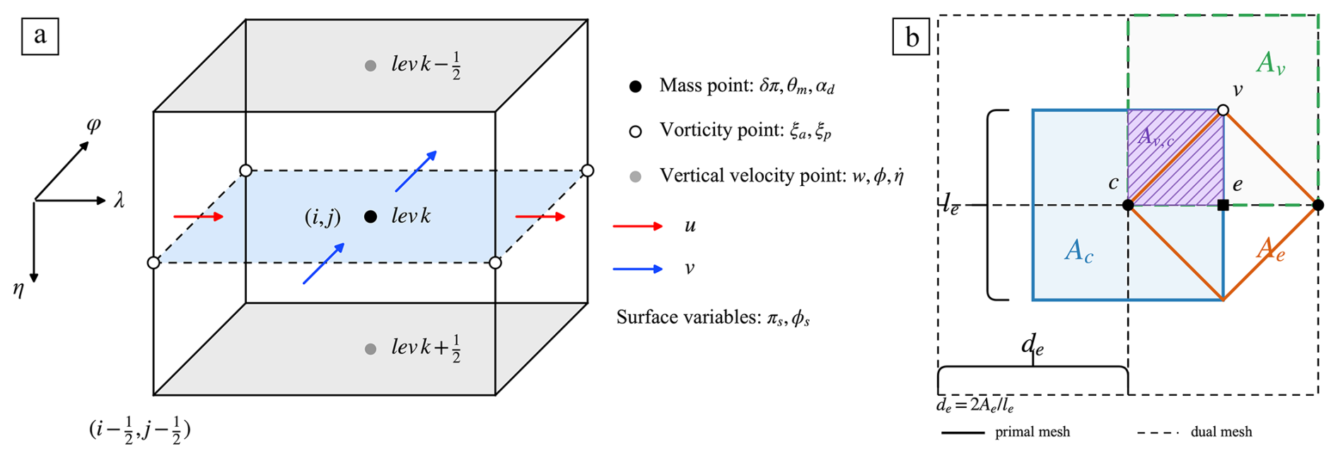
Figure 1 Schematic of the staggered-grid arrangement and the associated horizontal control volumes. The horizontal discretization uses an Arakawa C-grid and the vertical discretization uses Lorenz staggering. The black dot, open circles, and gray dots denote the mass point, vorticity points, and vertical-velocity points, respectively. Red and blue arrows denote the u and v wind components. The light-blue plane denotes the full level, and the gray planes denote the half levels. (b) Horizontal C-grid control-volume geometry around the edge and vertex locations. The primal mesh and dual mesh are shown by solid and dashed lines, respectively. The blue square denotes the cell-centered area A_c, the green dashed square denotes the vertex-associated area A_v, and the orange diamond denotes the edge-associated area A_e. The hatched region indicates the overlap area A_v,c between the vertex-associated and cell-centered control volumes. The characteristic edge length l_e and dual distance d_e are also indicated, with $d_e=\mathrm{2}{A}_e/l_e$.

Following Ringler et al. (2010), the subscripts c, e, and v denote a scalar-cell center, a velocity edge, and a vorticity vertex (the center of the corresponding dual control volume), respectively. In Fig. 1b, A_c and A_v are the primal- and dual-control-volume areas, l_e is the primal edge length, and d_e is the distance between the two neighboring cell centers sharing edge e. The sets E(c), C(e), E(v), C(v), and E_⟂(e) denote the edges around cell c, the two cells sharing edge e, the edges around vertex v, the cells surrounding vertex v, and the neighboring transverse edges of a target edge, respectively. The orientation factors $n_{e,c}=\pm \mathrm{1}$ and $t_{e,v}=\pm \mathrm{1}$ give the outward flux sign for a cell and the positive circulation sign around a vertex.

Let a be the reference planetary radius and r_c, r_e, and r_v the local radial distances at cell, edge, and vertex locations. A superscript (a) denotes the corresponding horizontal geometry on the reference sphere. The deep-atmosphere metric is therefore introduced directly through the local lengths and areas:

$$\begin{array}{}\text{(18)}& \begin{array}{rl}& l_e={\displaystyle \frac{r_e}{a}}{l}_e^{\left(a\right)},d_e={\displaystyle \frac{r_e}{a}}{d}_e^{\left(a\right)},\\ & A_c={\left({\displaystyle \frac{r_c}{a}}\right)}^{\mathrm{2}}{A}_c^{\left(a\right)},A_v={\left({\displaystyle \frac{r_v}{a}}\right)}^{\mathrm{2}}{A}_v^{\left(a\right)}.\end{array}\end{array}$$

The shallow-atmosphere form is recovered when $r_c=r_e=r_v=a$. Vertical transport uses the analogous shell-area factor ${\left(r/a\right)}^{\mathrm{2}}$ at layer interfaces.

For the basic finite-volume operators, F_e below denotes a generic edge-normal flux per unit edge length (distinct from the subgrid tendencies above). Its divergence at cell c is

$$\begin{array}{}\text{(19)}& {\left[\mathrm{\nabla }\cdot \mathit{F}\right]}_c={\displaystyle \frac{\mathrm{1}}{A_c}}\sum _{e\in E\left(c\right)}{n}_{e,c}{F}_e{l}_e.\end{array}$$

For a scalar q_c defined at cell centers, the edge-normal gradient is

$$\begin{array}{}\text{(20)}& {\left[\mathrm{\nabla }q\right]}_e={\displaystyle \frac{\mathrm{1}}{d_e}}\sum _{c\in C\left(e\right)}\left(-n_{e,c}\right)q_c={\displaystyle \frac{q_{c_{\mathrm{2}}}-q_{c_{\mathrm{1}}}}{d_e}},\end{array}$$

where c₁ and c₂ are the two cells in C(e), ordered along the oriented edge normal from c₁ to c₂. With V_e denoting the edge-normal wind component (u_e or v_e according to the edge orientation), the relative vorticity at vertex v is obtained from the circulation around the dual control volume:

$$\begin{array}{}\text{(21)}& {\mathit{\xi }}_v={\left[\widehat{\mathit{k}}\cdot \left(\mathrm{\nabla }\times \mathit{V}\right)\right]}_v={\displaystyle \frac{\mathrm{1}}{A_v}}\sum _{e\in E\left(v\right)}{t}_{e,v}{V}_e{d}_e,\end{array}$$

where $\widehat{\mathit{k}}$ is the local vertical unit vector. At the exact poles, GMCORE evaluates the same Stokes circulation over the complete polar cap (Li et al., 2020).

At a full model level, u_e and v_e denote the zonal and meridional wind components on their respective C-grid edges, w_e is the vertical velocity horizontally collocated with that edge, φ_e is the latitude. The semi-discrete horizontal momentum equations are:

$$\begin{array}{}\text{(22)}& {\displaystyle }\begin{array}{rl}{\displaystyle \frac{\partial u_e}{\partial t}}& =R_e^{\left(u\right)}-{\left[{\mathrm{\nabla }}_{\mathit{\eta }}K\right]}_e^{\left(u\right)}-\dot{\mathit{\eta }}{\displaystyle \frac{\partial u}{\partial \mathit{\eta }}}-L{\mathrm{PGF}}_{u_e}\\ & -\left(\mathrm{2}\mathrm{\Omega }\cos {\mathit{\phi }}_e+{\displaystyle \frac{u_e}{r_e}}\right)w_e+S,\end{array}\text{(23)}& {\displaystyle }\begin{array}{rl}{\displaystyle \frac{\partial v_e}{\partial t}}& =R_e^{\left(v\right)}-{\left[{\mathrm{\nabla }}_{\mathit{\eta }}K\right]}_e^{\left(v\right)}-\dot{\mathit{\eta }}{\displaystyle \frac{\partial v}{\partial \mathit{\eta }}}-L{\mathrm{PGF}}_{v_e}\\ & -{\displaystyle \frac{v_e{w}_e}{r_e}}+S.\end{array}\end{array}$$

Here $R_e^{\left(u\right)}$ and $R_e^{\left(v\right)}$ are the PV-flux rotational tendencies; K is the horizontal kinetic energy and ∇_η denotes the horizontal gradient on an η surface; ${\mathrm{PGF}}_{u_e}$ and ${\mathrm{PGF}}_{v_e}$ are the pressure-gradient forces; and S represents subgrid tendencies. The nontraditional Coriolis and curvature terms are kept explicitly in Eqs. (22) and (23).

The PV-flux rotational tendencies $R_e^{\left(u\right)}$ and $R_e^{\left(v\right)}$ in Eqs. (22) and (23) are evaluated as follows. Let δπ_c be the layer dry-air mass at cell c. The mass is interpolated to vertex v with the primal-dual overlap area weight A_v,c. The vertex layer mass and layer-mass potential vorticity are

$$\begin{array}{}\text{(24)}& \begin{array}{rl}& \mathit{\delta }{\mathit{\pi }}_v={\displaystyle \frac{\mathrm{1}}{A_v}}\sum _{c\in C\left(v\right)}{A}_{v,c}\mathit{\delta }{\mathit{\pi }}_c,{\mathit{\xi }}_{p,v}={\displaystyle \frac{{\mathit{\xi }}_v+f_v}{\mathit{\delta }{\mathit{\pi }}_v}},\\ & f_v=\mathrm{2}\mathrm{\Omega }\sin {\mathit{\phi }}_v.\end{array}\end{array}$$

Thus δπ_v is the layer mass collocated with the vorticity, f_v is the traditional Coriolis parameter, and ξ_p,v is the layer-mass potential vorticity.

At edge e, δπ_e is the mean layer mass of the two cells in C(e), V_e is the edge-normal wind, and F_e is the normal dry-mass flux. The transverse flux $F_e^{⟂}$ at the same target edge is reconstructed as

$$\begin{array}{}\text{(25)}& \begin{array}{rl}& F_e=\mathit{\delta }{\mathit{\pi }}_e{V}_e,\mathit{\delta }{\mathit{\pi }}_e={\displaystyle \frac{\mathrm{1}}{\mathrm{2}}}\sum _{c\in C\left(e\right)}\mathit{\delta }{\mathit{\pi }}_c,\\ & F_e^{⟂}={\displaystyle \frac{\mathrm{1}}{d_e}}\sum _{e^{\prime }\in E_{⟂}\left(e\right)}{\mathit{\omega }}_{e,e^{\prime }}{l}_{e^{\prime }}{F}_{e^{\prime }},\end{array}\end{array}$$

where e^′ runs over the four transverse neighbors in E_⟂(e), and ${\mathit{\omega }}_{e,e^{\prime }}$ is the corresponding geometric interpolation weight and we take ${\mathit{\omega }}_{e,e^{\prime }}=\frac{\mathrm{1}}{\mathrm{4}}$. This is the Ringler-type normal-to-transverse flux mapping used to collocate the mass flux with the rotational tendency.

GMCORE then reconstructs PV from the vertices to the target edge with its default third-order upwind stencil. Let v₋₁ and v₊₁ be the two nearest vertices on the two sides of edge e in the transverse direction and v₋₂, v₊₂ the next outward vertices. The reconstructed edge PV is

$$\begin{array}{}\text{(26)}& \begin{array}{rl}{\mathit{\xi }}_{p,e}^{\left(\mathrm{3}\right)}& ={\displaystyle \frac{\mathrm{7}}{\mathrm{12}}}\left({\mathit{\xi }}_{p,v_{+\mathrm{1}}}+{\mathit{\xi }}_{p,v_{-\mathrm{1}}}\right)-{\displaystyle \frac{\mathrm{1}}{\mathrm{12}}}\left({\mathit{\xi }}_{p,v_{+\mathrm{2}}}+{\mathit{\xi }}_{p,v_{-\mathrm{2}}}\right)\\ & +{\displaystyle \frac{{\mathit{\beta }}_{\mathrm{pv}}}{\mathrm{12}}}\mathrm{sgn}\left(F_e^{⟂}\right)[{\mathit{\xi }}_{p,v_{+\mathrm{2}}}-{\mathit{\xi }}_{p,v_{-\mathrm{2}}}\\ & -\mathrm{3}\left({\mathit{\xi }}_{p,v_{+\mathrm{1}}}-{\mathit{\xi }}_{p,v_{-\mathrm{1}}}\right)],\end{array}\end{array}$$

where β_pv controls the upwind contribution and $\mathrm{sgn}\left(F_e^{⟂}\right)$ selects the upstream side from the transverse mass flux. The PV-weighted rotational tendency is then

$$\begin{array}{}\text{(27)}& R_e={\mathit{\sigma }}_e{\displaystyle \frac{\mathrm{1}}{d_e}}\sum _{e^{\prime }\in E_{⟂}\left(e\right)}{\mathit{\omega }}_{e,e^{\prime }}{l}_{e^{\prime }}{F}_{e^{\prime }}{\displaystyle \frac{{\mathit{\xi }}_{p,e}^{\left(\mathrm{3}\right)}+{\mathit{\xi }}_{p,e^{{}^{\prime }\left(\mathrm{3}\right)}}}{\mathrm{2}}},\end{array}$$

where ${\mathit{\sigma }}_e=\pm \mathrm{1}$ accounts for the orientation of the zonal or meridional momentum equation, and ${\mathit{\xi }}_{p,e}^{\left(\mathrm{3}\right)}$ and ${\mathit{\xi }}_{p,e^{\prime \left(\mathrm{3}\right)}}$ are the third-order reconstructed PV values at the target and neighboring transverse edges. According to the edge orientation, R_e in Eq. (27) supplies $R_e^{\left(u\right)}$ or $R_e^{\left(v\right)}$ in Eqs. (22) and (23).

The kinetic energy is diagnosed at cell centers. Following Ringler et al. (2010) and the kinetic-energy reconstruction used by Gassmann (2013) and Skamarock et al. (2012), we define the edge-associated area $A_e=\frac{\mathrm{1}}{\mathrm{2}}{l}_e{d}_e$, the edge-based estimate $K_c^{\left(e\right)}$, the optional vertex-based estimate $K_c^{\left(v\right)}$, and the prescribed blending coefficient α_K:

$$\begin{array}{}\text{(28)}& \begin{array}{rl}& K_c^{\left(e\right)}={\displaystyle \frac{\mathrm{1}}{A_c}}\sum _{e\in E\left(c\right)}{A}_{c,e}{V}_e^{\mathrm{2}},\\ & K_v={\displaystyle \frac{\mathrm{1}}{A_v}}\sum _{e\in E\left(v\right)}{A}_{v,e}{V}_e^{\mathrm{2}},\\ & K_c^{\left(v\right)}={\displaystyle \frac{\mathrm{1}}{A_c}}\sum _{e\in V\left(c\right)}{A}_{v,c}{K}_v,\\ & K_c={\mathit{\alpha }}_K{K}_c^{\left(e\right)}+\left(\mathrm{1}-{\mathit{\alpha }}_K\right)K_c^{\left(v\right)}\end{array}\end{array}$$

Here, A_c,e and A_v,e are the portions of the edge-associated area assigned to the primal cell c and dual cell v, respectively, and V(c) denotes the vertices surrounding cell c. The vertex-based estimate $K_c^{\left(v\right)}$ is obtained by interpolating the vertex kinetic energy K_v to the cell center using the primal–dual overlap areas A_v,c. The blending coefficient α_K controls the contributions of the two estimates. In GMCORE, we take α_K=0.55 to suppress the potential Hollingsworth-type computational instability (Hollingsworth et al., 1983). The kinetic contribution at edge e is obtained with the same normal-gradient operator

$$\begin{array}{}\text{(29)}& {\left[\mathrm{\nabla }K\right]}_e={\displaystyle \frac{\mathrm{1}}{d_e}}\sum _{c\in C\left(e\right)}\left(-n_{e,c}\right)K_c={\displaystyle \frac{K_{c_{\mathrm{2}}}-K_{c_{\mathrm{1}}}}{d_e}},\end{array}$$

where $K_{c_{\mathrm{1}}}$ and $K_{c_{\mathrm{2}}}$ are the kinetic energies in the two cells adjacent to e. Because d_e already contains the local-radius scaling in Eq. (18), the deep-atmosphere metric enters this gradient directly.

Vertical momentum advection follows Simmons and Burridge (1981). At full level k, $M_{e,k+\frac{\mathrm{1}}{\mathrm{2}}}$ and $M_{e,k-\frac{\mathrm{1}}{\mathrm{2}}}$ are the dry-mass fluxes through the lower and upper interfaces, δπ_e,k is the layer dry-air mass at edge e, and V_e,k denotes either u_e,k or v_e,k. The operator is

$$\begin{array}{}\text{(30)}& {\left(\dot{\mathit{\eta }}{\displaystyle \frac{\partial V_e}{\partial \mathit{\eta }}}\right)}_k={\displaystyle \frac{M_{e,k+\frac{\mathrm{1}}{\mathrm{2}}}\left(V_{e,k+\mathrm{1}}-V_{e,k}\right)+M_{e,k-\frac{\mathrm{1}}{\mathrm{2}}}\left(V_{e,k}-V_{e,k-\mathrm{1}}\right)}{\mathrm{2}\mathit{\delta }{\mathit{\pi }}_{e,k}}}.\end{array}$$

The interface mass fluxes $M_{e,k+\frac{\mathrm{1}}{\mathrm{2}}}$ and $M_{e,k-\frac{\mathrm{1}}{\mathrm{2}}}$ are diagnosed from the same layer continuity equation, in the deep-atmosphere configuration each interface flux carries its own shell-area factor.

Finally, the horizontal pressure-gradient force is written in perturbation form to reduce cancellation on the terrain-following coordinate. Here p_c, ϕ_c, ${\mathit{\alpha }}_{d,c}=\mathrm{1}/{\mathit{\rho }}_{d,c}$, and π_c retain their definitions from Sect. 2.1; the subscript ref denotes a time-independent hydrostatically balanced reference state and a superscript prime denotes the perturbation from that state:

$$\begin{array}{}\text{(31)}& \begin{array}{rl}& p_c=p_{\mathrm{ref},c}+p_c^{\prime },{\mathit{\varphi }}_c={\mathit{\varphi }}_{\mathrm{ref},c}+{\mathit{\varphi }}_c^{\prime },\\ & {\mathit{\alpha }}_{d,c}={\mathit{\alpha }}_{d,\mathrm{ref},c}+{\mathit{\alpha }}_{d,c}^{\prime },{\mathit{\pi }}_c={\mathit{\pi }}_{\mathrm{ref},c}+{\mathit{\pi }}_c^{\prime }.\end{array}\end{array}$$

For any cell-centered quantity q_c, the overbar $\stackrel{\mathrm{‾}}{q_e}=\left(q_{c_{\mathrm{1}}}+q_{c_{\mathrm{2}}}\right)/\mathrm{2}$ denotes centered interpolation to edge e, while the bracketed gradients use Eq. (20). The symbol δ denotes the vertical increment across a model layer. The pressure-gradient force at an edge is

$$\begin{array}{}\text{(32)}& \begin{array}{rl}{\mathrm{PGF}}_e& ={\stackrel{\mathrm{‾}}{\mathit{\alpha }}}_{d,e}{\left[\mathrm{\nabla }{p}^{\prime }\right]}_e+{\stackrel{\mathrm{‾}}{\mathit{\alpha }}}_{d,e}^{\prime }{\left[\mathrm{\nabla }{p}_{\mathrm{ref}}\right]}_e\\ & +{\left[\mathrm{\nabla }{\mathit{\varphi }}^{\prime }\right]}_e+{\displaystyle \frac{\mathit{\delta }{p}_e^{\prime }-\mathit{\delta }{\mathit{\pi }}_e^{\prime }}{\mathit{\delta }{\mathit{\pi }}_e}}{\left[\mathrm{\nabla }\mathit{\varphi }\right]}_e.\end{array}\end{array}$$

The corresponding term in Eqs. (22) and (23) is −L PGF_e.

The model employs a centered difference scheme for layer-mass transport, while a third-order upwind scheme is adopted for potential temperature, geopotential, and vertical velocity. Tracer advection is handled by the SWIFT scheme (Bendall and Kent, 2025), which is derived from the FFSL formulation (Lin and Rood, 1996) with specific modifications to preserve monotonicity in two-dimensional transport and relies on PPM for the spatial reconstruction of tracers.

A challenge for latitude-longitude grids is the severe convergence of meridians at the poles, which typically induces numerical noise and structural deformation in cross-polar flows. To circumvent this singularity, GMCORE redefines the relative vorticity around the poles via Stokes' theorem (Li et al., 2020). This specific physical constraint governs the evolution of potential enstrophy, effectively suppressing artificial computational noise sources precisely at the polar singularities.

2.4 Time integration: semi-implicit scheme

After the spatial discretization described in Sect. 2.3, the governing equations can be written in the following prototype form:

$$\begin{array}{}\text{(33)}& {\displaystyle \frac{\partial \mathit{X}}{\partial t}}=-\mathcal{L}\left(\mathit{X}\right),\end{array}$$

where X represents any prognostic variable and ℒ(X) denotes the corresponding spatially discretized tendency, including the terms described in Sect. 2.3. GMCORE advances Eq. (33) using a modified three-stage Runge–Kutta scheme (Wicker and Skamarock, 2002). Starting from the model state Xⁿ at time level n, the three stages are

$$\begin{array}{}\text{(34a)}& {\displaystyle }{\mathit{X}}^{*}={\mathit{X}}^n-{\displaystyle \frac{\mathrm{\Delta }t}{\mathrm{3}}}\mathcal{L}\left({\mathit{X}}^n\right),\text{(34b)}& {\displaystyle }{\mathit{X}}^{**}={\mathit{X}}^n-{\displaystyle \frac{\mathrm{\Delta }t}{\mathrm{2}}}\mathcal{L}\left({\mathit{X}}^{*}\right),\text{(34c)}& {\displaystyle }{\mathit{X}}^{n+\mathrm{1}}={\mathit{X}}^n-\mathrm{\Delta }t\mathcal{L}\left({\mathit{X}}^{**}\right),\end{array}$$

where Δt is the dynamical time step, X^* and ${\mathit{X}}^{**}$ denote the intermediate states of the first and second Runge–Kutta stages, respectively, and Xⁿ⁺¹ is the updated state. At each stage, the spatial tendency is recomputed using the most recently obtained intermediate state, whereas the stage update is based on Xⁿ. Thus, the three evaluations of the spatial operator are successively performed at Xⁿ, X^*, and ${\mathit{X}}^{**}$.

Each Runge–Kutta stage can be regarded as a forward-in-time update over the corresponding stage interval. Within such an update, most dycore tendencies are evaluated explicitly, whereas the vertically propagating fast acoustic modes require a different treatment. When using the nonhydrostatic solver, the vertical momentum and geopotential equations (in Eqs. 2 and 6) form a vertically coupled subsystem: w is coupled to the vertical pressure-gradient force, while ϕ evolves directly with w, and the pressure response is linked to them through the equation of state.

Following the vertical implicit treatment used in nonhydrostatic models GRIST (Zhang et al., 2019) and ICON (e.g., Zängl et al., 2015), the prognostic variables are computed directly as full-field quantities without relying on a stationary, global background reference profile.

In this semi-implicit formulation, horizontal advection, vertical advection and the full Coriolis force are evaluated explicitly. Conversely, the terms responsible for high-frequency vertical acoustic wave propagation – specifically the vertical pressure gradient force in the vertical momentum equation, and the associated w⋅g(r) term in the geopotential equation – are treated implicitly. By introducing an off-centering weight $\mathit{\beta }\in \left[\mathrm{0.5},\mathrm{1.0}\right]$, the implicit equations for the vertical velocity w and the geopotential ϕ can be conceptually simplified as:

$$\begin{array}{}\text{(35)}& {\displaystyle }{w}^{\mathit{\tau }}=\mathrm{\Delta }\mathit{\tau }\cdot R_w^{*}+\mathit{\beta }\mathrm{\Delta }\mathit{\tau }L{g}_{\mathrm{0}}{\left({\displaystyle \frac{r}{a}}\right)}^{\mathrm{2}}{\displaystyle \frac{\mathit{\delta }\left(p^{\mathit{\tau }}\right)}{\mathit{\delta }\left({\mathit{\pi }}^{\mathit{\tau }}\right)}},\text{(36)}& {\displaystyle }{\mathit{\varphi }}^{\mathit{\tau }}=\mathrm{\Delta }\mathit{\tau }\cdot R_{\mathit{\varphi }}^{*}+\mathit{\beta }\mathrm{\Delta }\mathit{\tau }{g}_{\mathrm{0}}{\left({\displaystyle \frac{a}{r}}\right)}^{\mathrm{2}}{w}^{\mathit{\tau }},\end{array}$$

where $R_w^{*}$ and $R_{\mathit{\varphi }}^{*}$ represent the total explicit residual tendencies evaluated at time stage * and Δτ is the sub-timestep. At full levels, the temporal increment of pressure $p^{\mathit{\tau }}-p^{*}$ is diagnostically linked to vertical increment of δϕ and the thermodynamic properties through the linearized equation of state:

$$\begin{array}{}\text{(37)}& {\displaystyle \frac{p^{\mathit{\tau }}-p^{*}}{p^{*}}}\approx \mathit{\gamma }\left({\displaystyle \frac{{\left(\mathit{\delta }\mathit{\pi }{\mathit{\theta }}_{\mathrm{m}}\right)}^{\mathit{\tau }}}{{\left(\mathit{\delta }\mathit{\pi }{\mathit{\theta }}_{\mathrm{m}}\right)}^{*}}}-{\displaystyle \frac{\mathit{\delta }\left({\mathit{\varphi }}^{\mathit{\tau }}\right)}{\mathit{\delta }\left({\mathit{\varphi }}^{*}\right)}}\right),\end{array}$$

where $\mathit{\gamma }=c_p/c_v$ is the ratio of the specific heats at constant pressure and constant volume, Eq. (37) can be discretized in the vertical:

$$\begin{array}{}\text{(38)}& \mathit{\delta }\left(p^{\mathit{\tau }}\right)=\mathit{\delta }\left(p^{*}\right)+\mathit{\gamma }\mathit{\delta }\left(p^{*}{\displaystyle \frac{{\left(\mathit{\delta }\mathit{\pi }{\mathit{\theta }}_{\mathrm{m}}\right)}^{\mathit{\tau }}}{{\left(\mathit{\delta }\mathit{\pi }{\mathit{\theta }}_{\mathrm{m}}\right)}^{*}}}\right)-\mathit{\gamma }\mathit{\delta }\left(p^n{\displaystyle \frac{\mathit{\delta }\left({\mathit{\varphi }}^{\mathit{\tau }}\right)}{\mathit{\delta }\left({\mathit{\varphi }}^{*}\right)}}\right).\end{array}$$

By substituting the implicit geopotential relation in Eq. (36) into Eq. (38), and then substituting the resulting pressure increment into the vertical momentum equation, Eq. (35), we eliminate the dependencies on other prognostic variables. This procedure reduces the coupled equations into a one-dimensional vertical equation for the vertical velocity w within each independent grid column. When discretized on the vertically staggered levels, it directly forms a standard tri-diagonal linear system:

$$\begin{array}{}\text{(39)}& A_{k-\frac{\mathrm{1}}{\mathrm{2}}}{w}_{k-\frac{\mathrm{1}}{\mathrm{2}}}^{\mathit{\tau }}+B_{k+\frac{\mathrm{1}}{\mathrm{2}}}{w}_{k+\frac{\mathrm{1}}{\mathrm{2}}}^{\mathit{\tau }}+C_{k+\frac{\mathrm{3}}{\mathrm{2}}}{w}_{k+\frac{\mathrm{3}}{\mathrm{2}}}^{\mathit{\tau }}=R_{w,k+\frac{\mathrm{1}}{\mathrm{2}}}^{*},\end{array}$$

where $R_{w,k+\frac{\mathrm{1}}{\mathrm{2}}}^{*}$ includes all the explicitly resolved forcing terms. The matrix coefficients $A_{k-\frac{\mathrm{1}}{\mathrm{2}}},B_{k+\frac{\mathrm{1}}{\mathrm{2}}}$, and $C_{k+\frac{\mathrm{3}}{\mathrm{2}}}$ are dynamically updated at each time step based on the local atmospheric state.

This one-dimensional tri-diagonal system is solved independently for every vertical column using the highly efficient Thomas algorithm, demanding no horizontal communication. Once the vertical velocity w is obtained, the increments for the remaining implicitly treated variables (such as δϕ and δp) are sequentially back-substituted. This semi-implicit vertical nonhydrostatic solver successfully decouples the fast vertical acoustic wave speeds from the integration stability criteria. This approach allows GMCORE to avoid solving global elliptic equations during nonhydrostatic calculations and to increase the time step.

2.5 Polar filtering and damping

Due to the convergence of the latitude and longitude grids at the poles, the zonal grid spacing shrinks significantly in the polar regions. As a result, the local zonal CFL number increases sharply in the polar region and can impose a severe stability constraint on the explicit part of the dynamical time integration.

In GMCORE, we apply an adaptive zonal gaussian convolution filter for dynamical tendencies along each latitude circle. For an arbitrary tendency field M in $u,v,{\mathit{\theta }}_{\mathrm{m}},{\mathit{\pi }}_{\mathrm{s}}$ and advection tendency of w,ϕ in nonhydrostatic module, the filtered field M^filt can be written

$$\begin{array}{}\text{(40)}& M_{i,j,k}^{\mathrm{filt}}=\sum _{m=-H_j}^{H_j}{G}_{j,m}{M}_{i+m,j,k},\end{array}$$

where G_j,m is the gaussian weight at offset m on the jth latitude circle, and H_j is the corresponding half-width of the stencil. Because the zonal direction is periodic, the index i+m is wrapped cyclically around the latitude circle.

The kernel width is not prescribed as a constant but diagnosed adaptively from the local zonal stability constraint. In the implementation, a dimensionless width parameter is first defined as

$$\begin{array}{}\text{(41)}& W_j={\mathit{\alpha }}_{\mathrm{f}}{\displaystyle \frac{c_{\mathrm{f}}\mathrm{\Delta }t}{\mathrm{\Delta }{x}_j}},\end{array}$$

where Δx_j is the zonal grid spacing on latitude ϕ_j, Δt is the dynamical time step, and c_f is a characteristic filtering wave speed now set to 300 m s⁻¹. The coefficient α_f is the parameter controlling the overall filter strength. The factor $\frac{c_{\mathrm{f}}\mathrm{\Delta }t}{\mathrm{\Delta }{x}_j}$ has the form of a zonal CFL number, so that the filter automatically becomes stronger where the grid is more restrictive. This latitude-dependent feature provides a smooth transition of the kernel width with latitude and helps avoid abrupt changes in filtering strength.

The diagnosed continuous width W_j is converted to the discrete stencil size by taking the smallest odd integer not smaller than W_j, with a minimum stencil size of three grid points: $N_j=max\left[\mathrm{3},\mathrm{oddceil}\left(W_j\right)\right]$.The continuous kernel is represented on the discrete stencil through a gaussian profile. For a stencil of width $N_j=\mathrm{2}{H}_j+\mathrm{1}$, the unnormalized weights are defined by

$$\begin{array}{}\text{(42)}& {\stackrel{\mathrm{̃}}{G}}_{j,m}={\displaystyle \frac{\mathrm{1}}{s_j\sqrt{\mathrm{2}\mathit{\pi }}}}\exp \left(-{\displaystyle \frac{m^{\mathrm{2}}}{\mathrm{2}{s}_j^{\mathrm{2}}}}\right),m=-H_j,\mathrm{\dots },H_j,\end{array}$$

with $s_j=\frac{W_j}{{\mathit{\sigma }}_{\mathrm{f}}}$ , where σ_f is a prescribed shape parameter controlling the relation between the diagnosed width W_j and the standard deviation of the discrete gaussian kernel. The final gaussian filter weights are then normalized as

$$\begin{array}{}\text{(43)}& G_{j,m}={\stackrel{\mathrm{̃}}{G}}_{j,m}/\sum _{m=-H_j}^{H_j}{\stackrel{\mathrm{̃}}{G}}_{j,m},\sum _{m=-H_j}^{H_j}{G}_{j,m}=\mathrm{1}.\end{array}$$

The normalization procedure guarantees that the filter preserves constant fields. In this way, the filter automatically strengthens near the poles while remaining weak in lower latitudes. Because the method uses only finite-width local convolution, it avoids the global communication required by FFT-based polar filtering and is therefore well suited to parallel latitude–longitude grid implementations. It should be noted that the wider communication halo is required only for the variables to which the filter is applied. In the parallel implementation, processes covering higher latitudes therefore use wider halos for those variables. In practice with a horizontal resolution of 1°, this half width halo usually reaches 90 points at the two poles of north and south. Nevertheless, the additional communication cost remains manageable for the resolutions considered here.

In addition to the polar gaussian filter, GMCORE applies optional horizontal divergence damping to the momentum field (Lauritzen et al., 2011). This damping is to diffuse the divergent part of flow noise that may otherwise accumulate near steep gradients, in the upper levels, or in the polar region. The damping is formulated in terms of the horizontal divergence, let

$$\begin{array}{}\text{(44)}& {\mathit{\delta }}_h={\mathrm{\nabla }}_h\cdot \mathit{V},\end{array}$$

where $\mathit{V}=\left(u,v\right)$ is the wind vector. δ_h is the divergence. The second-order divergence damping is written as

$$\begin{array}{}\text{(45)}& {\left.{\displaystyle \frac{\partial \mathit{V}}{\partial t}}\right|}_{\mathit{\delta },\mathrm{2}}={\mathit{\nu }}_{\mathit{\delta },\mathrm{2}}{\mathrm{\nabla }}_h{\mathit{\delta }}_h,\end{array}$$

and a more scale-selective fourth-order option is

$$\begin{array}{}\text{(46)}& {\left.{\displaystyle \frac{\partial \mathit{V}}{\partial t}}\right|}_{\mathit{\delta },\mathrm{4}}=-{\mathit{\nu }}_{\mathit{\delta },\mathrm{4}}{\mathrm{\nabla }}_h{\mathrm{\nabla }}_h^{\mathrm{2}}{\mathit{\delta }}_h.\end{array}$$

The damping coefficients ν_δ,2 and ν_δ,4 are scaled with the local grid area and time step and can be smoothly enhanced near the poles or upper levels.

$$\begin{array}{}\text{(47)}& {\mathit{\nu }}_{\mathit{\delta },\mathrm{2}}\sim C_{\mathrm{2}}{\displaystyle \frac{A}{\mathrm{\Delta }t}},{\mathit{\nu }}_{\mathit{\delta },\mathrm{4}}\sim C_{\mathrm{4}}{\displaystyle \frac{A^{\mathrm{2}}}{\mathrm{\Delta }t}}.\end{array}$$

GMCORE also provides an optional upper-level Rayleigh damping of vertical velocity. This damping is not activated in the two idealized cases presented here; with their comparatively low model tops, both cases remain numerically stable without a sponge layer. For future high-top applications, the same damping option can be used as an upper-boundary treatment to attenuate upward-propagating disturbances and reduce artificial reflection, rather than as a correction to the deep-atmosphere equations themselves.

3 Test cases and simulation results

To test the validity and performance of deep-atmosphere version of GMCORE, particularly the deep-atmosphere modifications described in Sect. 2, two standard idealized test cases are selected.

3.1 Deep-atmosphere baroclinic wave

The idealized baroclinic wave test case evaluates the model's ability to simulate mid-latitude baroclinic processes. Following the model parameters proposed by Ullrich et al. (2014), we employ this test to demonstrate the characteristics of the deep-atmosphere configurations. The simulations use the 30-level vertical grid adopted from CAM, with the model top located at 2.255 hPa, corresponding to an approximate geometric height of 30 km. The horizontal resolution is 1°, corresponding to a 360 × 180 regular latitude–longitude grid. The domain is decomposed along the latitude direction for parallel computation. The simulations were performed using 2 compute nodes with 120 CPU cores in total, and the wall-clock time for the integration reported here was approximately 5 min.

The initial conditions feature a mid-latitude jet in hydrostatic and geostrophic balance (Staniforth and White, 2011), which is subsequently perturbed to trigger baroclinic instability. Before the baroclinic simulation, the barotropic steady geostrophic flow (see Williamson et al., 1992, their test Case2) is employed, for which an analytical solution is available to verify the convergence of GMCORE. Another reason for adopting this barotropic test case is to avoid the non-convergence issues that may arise from initialization in a three-dimensional baroclinic model. We then use the unperturbed standard-Earth baroclinic-wave basic state to examine the stability of GMCORE.

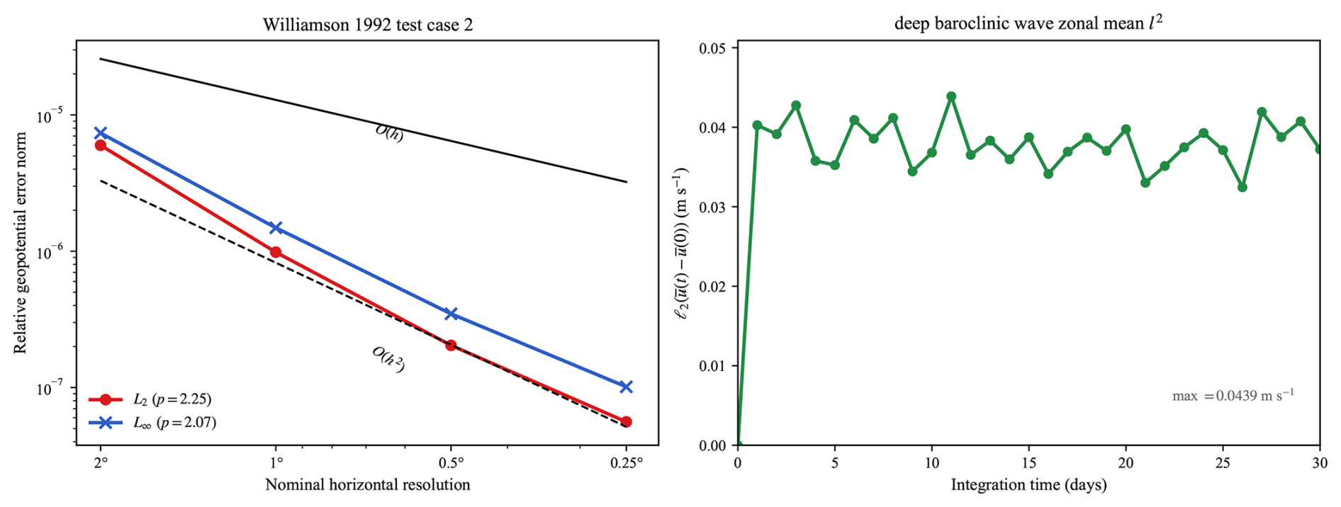
Figure 2 Convergence and stability diagnostics of GMCORE. The left panel presents the relative (L₂) and (L_∞) geopotential error norms for Williamson 1992 test case 2 at resolutions from 2 to 0.25°, with reference O(h) and O(h²) slopes. The right panel shows the (l²) norm of the zonal-mean wind deviation from its initial state in the unperturbed deep baroclinic-wave basic-state test, demonstrating a bounded drift over 30 d.

Steady geostrophic flow is integrated for 5 d at nominal horizontal resolutions of 2, 1, 0.5, and 0.25°, with time steps of 600, 300, 150, and 75 s, respectively. The fitted convergence orders of the relative geopotential errors are 2.25 for L² and 2.07 for L^∞, indicating near-second-order convergence (in the left panel of Fig. 2). For the three-dimensional model, stability is tested using the unperturbed standard-Earth baroclinic-wave basic state. Following Jablonowski and Williamson (2006), we monitor the weighted norms $l_{\mathrm{2}}\left(\stackrel{\mathrm{‾}}{u}\left(t\right)-\stackrel{\mathrm{‾}}{u}\left(\mathrm{0}\right)\right)$. On the 1° grid, the norm remains below 0.044 m s⁻¹ throughout the 30 d integration, indicating stable preservation of the balanced basic state (in the right panel of Fig. 2).

Simulations with perturbation are conducted using both the deep-atmosphere and the shallow-atmosphere solvers. Figure 3 shows the evolution of surface pressure, 850 hPa temperature, and 850 hPa relative vorticity in the deep configuration at days 8 and 10. The developing wave exhibits the familiar life cycle of baroclinic instability: a midlatitude disturbance grows along the jet, amplifies downstream, and evolves into a mature cyclone–anticyclone structure. Overall, the simulated fields are consistent with the standard behaviour reported in previous model intercomparisons of this test case (Ullrich et al., 2014; Wood et al., 2014; Borchert et al, 2019; Skamarock et al., 2021; Kelly et al., 2026; Yatunin et al., 2026), and indicate that the GMCORE deep-atmosphere dycore is able to maintain the balanced basic state and reproduce the expected evolution of the wave under Earth-like conditions.

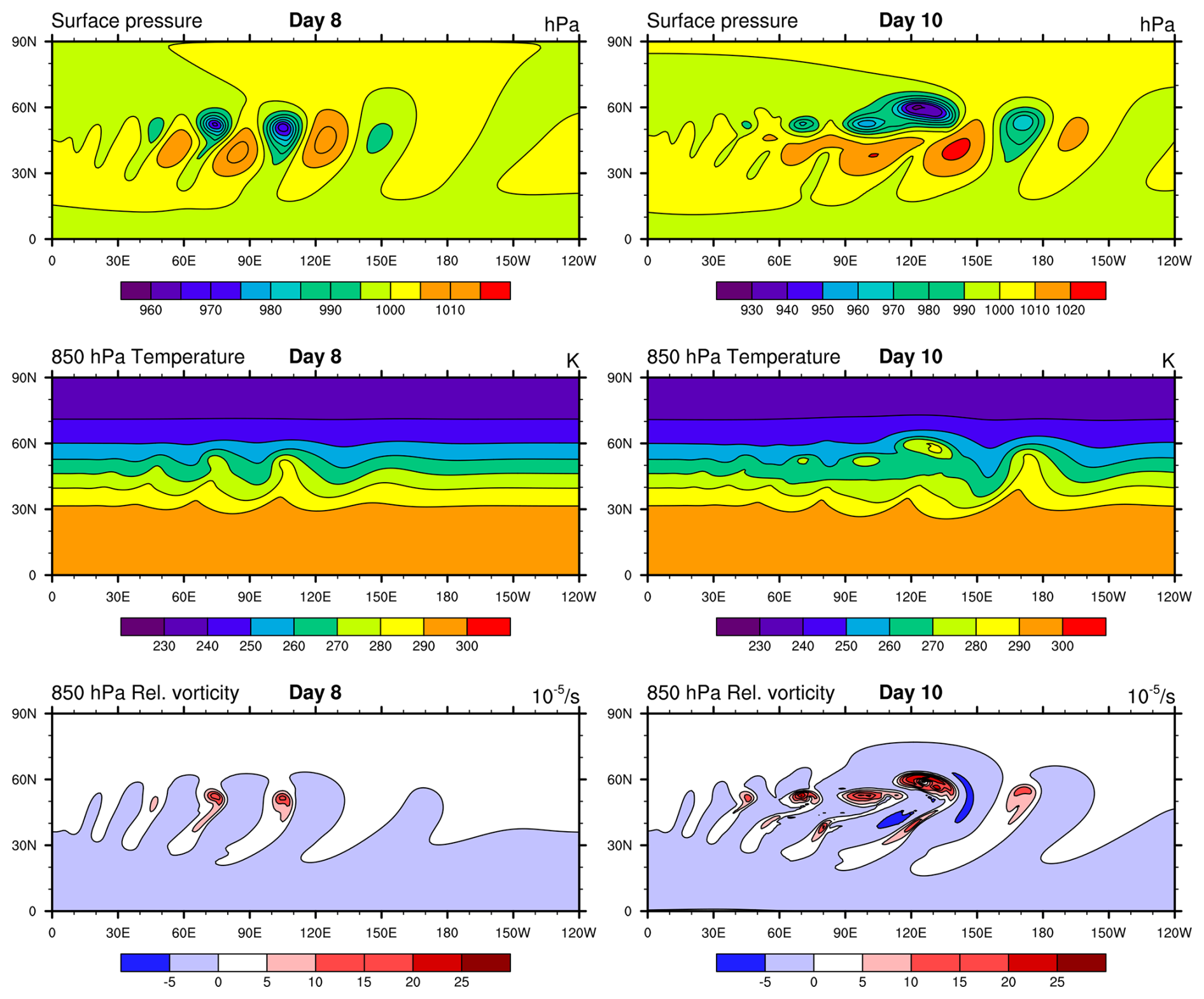
Figure 3 Evolution of the surface pressure, 850 hPa temperature and relative vorticity for the deep baroclinic wave test at days 8 and 10. These can be compared with Ullrich et al.'s (2014) Figs. 4 and 5, and with Skamarock et al.'s (2021) Fig. 2.

With a timestep of 300 s, the gravity-wave CFL number is approximately 0.27 near the equator, 0.39 at midlatitudes, and 0.64 at 60°. It exceeds unity poleward of about 70° because of the reduced zonal grid spacing, while the gaussian filter is adaptively strengthened according to Eq. (41). Vertical acoustic terms are treated semi-implicitly to relax their CFL constraint.

In a standard Earth-radius experiment (a≈6371 km), the troposphere is extremely thin relative to the planet's radius. Consequently, the deep-atmosphere geometrical scaling ${\left(r/a\right)}^{\mathrm{2}}$ and the variable gravity g(r) introduce very small dynamical differences compared to the shallow-atmosphere.

To amplify the dynamical differences between the deep- and shallow-atmosphere equations, we follow Ullrich et al. (2014) and employ the reduced-radius, or “small-Earth”, baroclinic-wave experiment, in which the planetary radius is decreased by a factor of 20 while the planetary angular rotation velocity is increased by the same factor. Under the standard Earth-radius experiment, the two experiments produce nearly indistinguishable baroclinic-wave evolutions, whereas in the X20 experiment the shallow-atmosphere assumption is no longer strictly valid and the two solutions separate much more clearly.

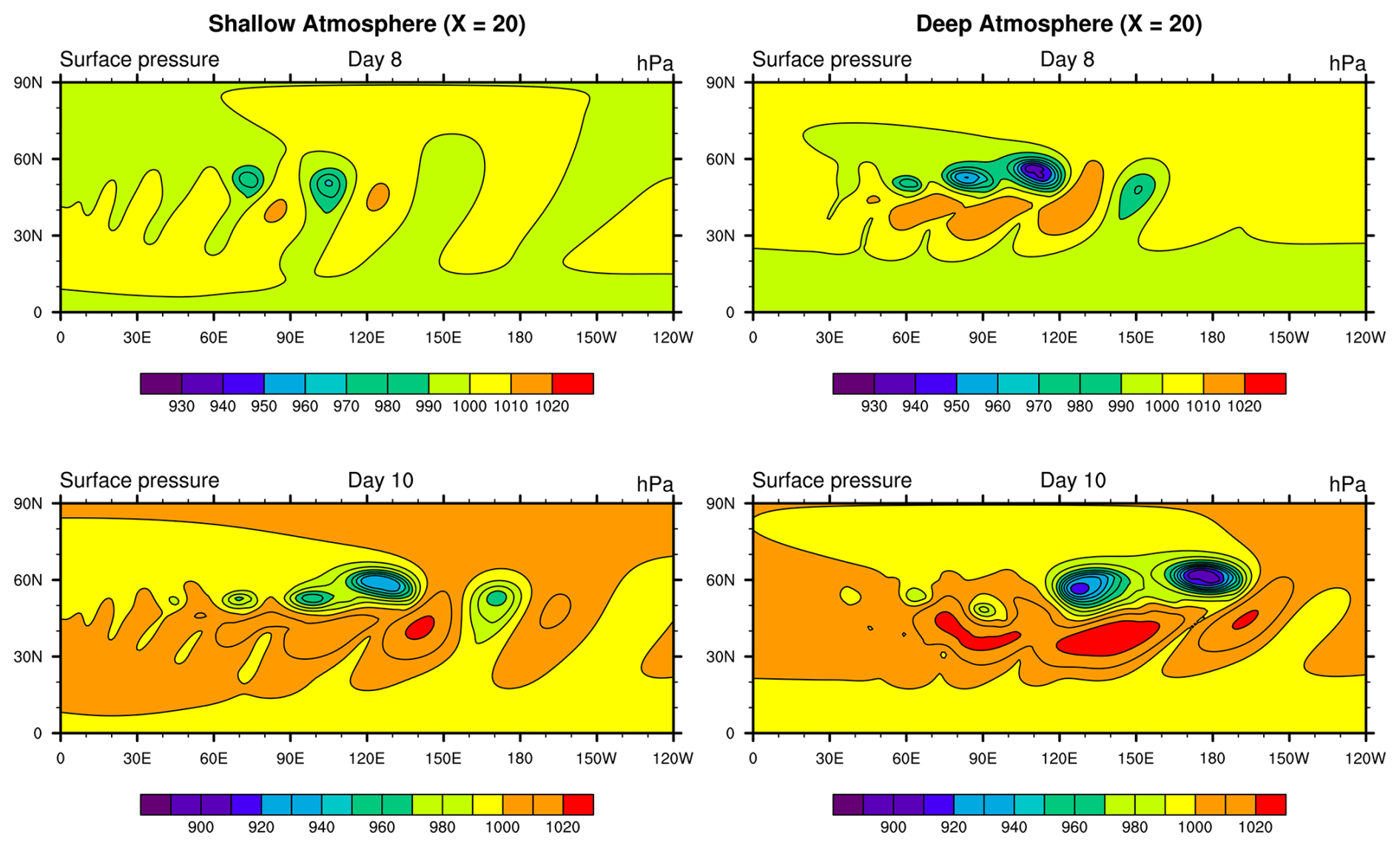
Figure 4 Surface pressure fields in the X20 reduced-radius baroclinic-wave experiment for the shallow-atmosphere and deep-atmosphere configurations at days 8 and 10. Following Ullrich et al. (2014), the planetary radius is reduced by a factor of 20 and the planetary angular rotation velocity is increased by the same factor in order to exaggerate the differences between the two equation sets. These can be compared with Fig. 9 in Ullrich et al. (2014), Fig. 6 in Borchert et al.'s (2019) and Fig. 6 in Skamarock et al.'s (2021).

In our X20 simulations, the shallow-atmosphere solution retains a comparatively weaker and smoother baroclinic-wave structure, broadly consistent with the reference behaviour reported by Ullrich et al. (2014). In contrast, the deep-atmosphere solution exhibits a more rapid amplification of the wave and a substantially stronger cyclonic development. By day 8, the deep-atmosphere field already shows a more compact and intense low-pressure center together with a more amplified downstream wave; by day 10, the contrast becomes even more pronounced, with the deep-atmosphere solution characterized by a deeper and stronger mature cyclone, while the shallow-atmosphere counterpart remains less developed. This behaviour is consistent with Ullrich et al. (2014), who showed that in the X20 experiment the deep-atmosphere integration intensifies much more rapidly and drives the minimum surface pressure below 900 hPa by day 10, whereas the shallow-atmosphere result remains much closer to the standard baroclinic-wave evolution.

To sum up, the numerical consistency tests and the baroclinic-wave experiments serve complementary purposes. The steady geostrophic-flow test shows near-second-order convergence, while the unperturbed standard-Earth basic state remains close to its balanced state throughout the 30 d integration. For the perturbed baroclinic wave, the deep- and shallow-atmosphere solutions are nearly indistinguishable under the standard-Earth-radius setup but separate clearly in the X20 reduced-radius experiment, consistent with published deep-atmosphere benchmarks. Because part of the X20 contrast may originate from differences in the analytic initial states, we regard this experiment primarily as a benchmark-reproduction test rather than as a quantitative attribution of the deep-atmosphere terms. Together, these results provide complementary evidence for the numerical consistency and correctness of the GMCORE deep-atmosphere implementation.

3.2 Tropical cyclone simulation

Next, we try to use an idealized tropical cyclone (TC) test case, which was proposed by Reed and Jablonowski (2011). In this case, an initial warm-core vortex that satisfies gradient wind balance is inserted in an aquaplanet without topography. This eliminates the land surfaces and the real environmental flow effects, making it an ideal test-bed for isolating and evaluating the deep-atmosphere modification. More precisely, due to the low model top (about 30 km) of this case, geometric and variable-gravity effects are expected to be much smaller than the retained nontraditional Coriolis contribution. This case is therefore used mainly to examine the impact of the NCTs-related deep-atmosphere terms.

We follow the standard setup of Reed and Jablonowski (2011) and run this case at a horizontal resolution of 0.25 and 0.125° for 10 d with the same vertical grid as the baroclinic-wave. The 0.25° simulations were performed using 480 CPU cores with a walltime around 120 min, whereas the 0.125° simulations used 600 CPU cores with a walltime around 900 min. To isolate the dynamical impact of the deep-atmosphere terms, the experiment is executed using both the nonhydrostatic deep-atmosphere (NHD) and nonhydrostatic shallow-atmosphere (NHS) configurations.

3.3 Tropical cyclone trajectories comparison

During the dynamical evolution of a tropical cyclone, the full three-dimensional Coriolis force – specifically the NCTs – is conventionally neglected in traditional shallow-atmosphere models. However, in the deep tropics where cosφ approaches its maximum, and within the TC eyewall region characterized by exceptionally strong vertical updrafts (with w frequently exceeding 10 m s⁻¹), the horizontal and vertical momentum forcings generated by the NCTs become non-negligible in magnitude. Although previous idealized cloud-resolving studies (e.g., Igel and Biello, 2020) have highlighted the potential impact of NCTs on equatorial convection, the macroscopic dynamical effects of this mechanism within a global deep-atmosphere dycore during a complete TC life cycle remain largely unverified.

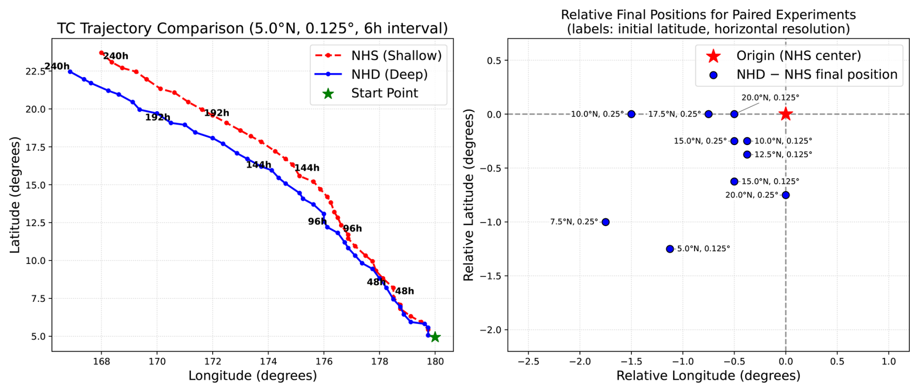
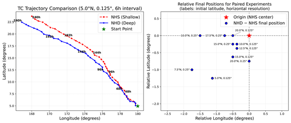
Figure 5 Simulated tropical cyclone trajectories for the nonhydrostatic shallow-atmosphere (NHS, red line) and nonhydrostatic deep-atmosphere (NHD, blue line) configurations at a horizontal resolution of 0.125°. The left panel shows the 10 d trajectories for the experiment initialized at 5° N. In the right panel, each blue dot shows the NHD − NHS difference in final storm-center position at 240 h for one independent paired experiment, after translating the corresponding NHS center to (0, 0). Labels indicate the initial perturbation latitude and horizontal resolution; the dots do not represent a time series. Storm centers are diagnosed directly from the grid-point minimum of surface pressure.

As shown in Fig. 5a, both NHS and NHD simulations produce a north-westward-moving tropical cyclone, but the NHD trajectory exhibits a systematic south-westward displacement relative to the NHS trajectory as the vortex develops. This result is qualitatively similar to that reported by Liang and Chan (2005), who found that inclusion of the 2Ωcosφw term had little effect on tropical-cyclone intensity but led to a westward to south-westward trajectory deviation. We also test different perturbations at different latitudes and get the same conclusion (Fig. 5b).

In our results, both simulations remain similar in terms of storm intensity and axisymmetric structure. As already indicated in the Supplementary Material, the two simulations show no essential difference in the minimum central pressure, maximum low-level wind speed, or the warm-core structure, suggesting that the leading-order thermodynamic processes controlling storm intensification are not strongly altered by the deep-atmosphere extension.

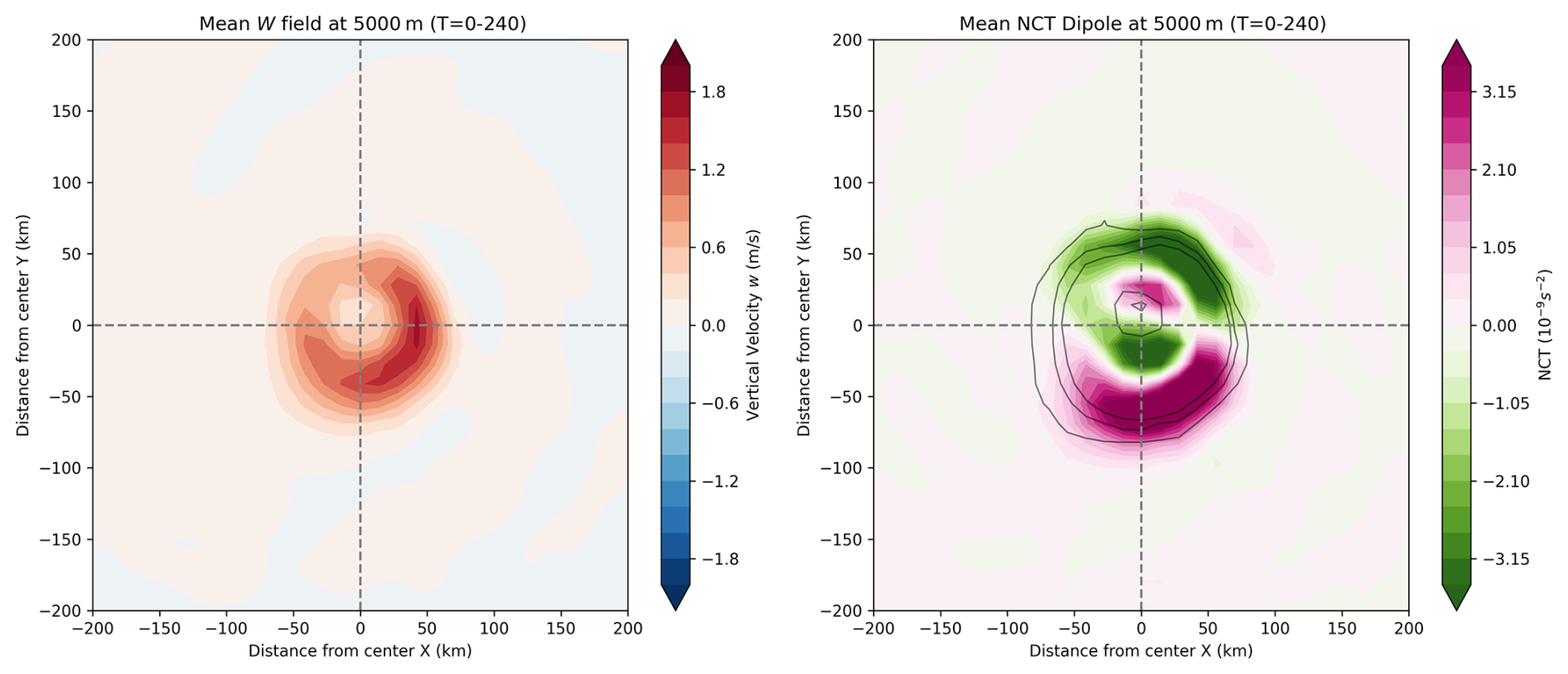
Figure 6 Horizontal cross-sections of time-averaged (T = 0–240 h) atmospheric variables at an altitude of 5000 m. (Left) Mean vertical velocity (w) field (m s⁻¹), illustrating a core of intense upward motion centered at the origin. (Right) Mean NCTs dipole (10⁻⁹ s⁻²), showing a distinct positive (pink) and negative (green) coupled structure near the vortex core. Both panels are centered on the system's axis, with distances indicated in kilometers from the center (x,y). The center is first identified within a neighbourhood of the storm position at the preceding output time. A two-dimensional quadratic surface is then fitted to the surrounding 5×5 grid points, and the local minimum of the fitted surface is used as the sub-grid storm center.

To interpret this trajectory difference, Fig. 6 shows the time-mean horizontal structure at 5 km altitude. In Fig. 6a, the mean vertical velocity field exhibits a compact core of strong ascent near the storm center. This indicates that the mature vortex maintains a well-defined eyewall-like updraft region. Closely collocated with this convective core, in Fig. 6b, we show the quantity

$$\begin{array}{}\text{(48)}& \mathrm{\Gamma }=\mathrm{2}\mathrm{\Omega }\cos \mathit{\phi }{\displaystyle \frac{\partial w}{\partial y}},\end{array}$$

which represents the vorticity tendency associated with the NCTs in the x-momentum equation. Here, the dipole-like structure refers to the pair of opposite-signed Γ anomalies on the two sides of the storm center. In other words, the meridional gradient of the eyewall vertical motion produces a positive tendency on one side of the core and a negative tendency on the other, giving rise to an organized inner-core asymmetry rather than an axisymmetric distribution.

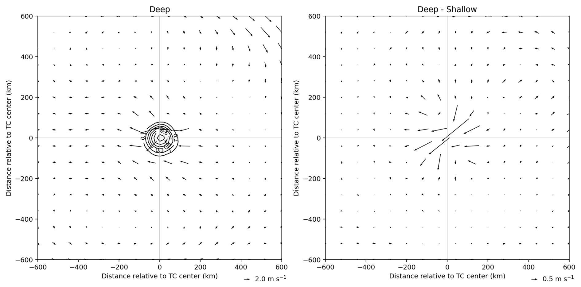
Figure 7 Horizontal wind velocity vectors and vertical velocity contours at an altitude of 1500 m. (Left) NHD wind field, showing a cyclonic circulation with a localized maximum in wind speed (contours, m s⁻¹) near the Tropical Cyclone (TC) center. Reference vector indicates a magnitude of 2.0 m s⁻¹. (Right) Difference in wind velocity between the NHD and NHS cases (NHD − NHS). This panel highlights the variation in environmental flow and the intensity of the low-level circulation between the two experiments, with a reference vector of 0.5 m s⁻¹. All coordinates are relative to the TC center (km).

This dipole is dynamically consistent with the near-core easterly anomaly shown in Fig. 7, which in turn is consistent with the south-westward displacement of the NHD trajectory. Figure 7 shows the horizontal winds at 1.5 km. The left panel gives the circulation in the NHD run, and the right panel shows the wind difference between the deep and shallow simulations. The main feature in the difference field is an easterly anomaly near the storm center. This anomaly is important because it is consistent with the south-westward displacement of the NHD trajectory in Fig. 5. In the Liang and Chan (2005) experiments, the additional Coriolis term associated with vertical motion produced a generally easterly flow near the TC center, and this easterly flow was identified as the immediate cause of the westward or south-westward displacement. Our result is not identical to their diagnosis, but the low-level easterly anomaly in Fig. 7 points in the same direction. It suggests that the south-westward shift in the NHD trajectory is tied to a coherent change in the inner-core flow rather than to random differences accumulated during the integration.

At the same time, the present analysis remains more limited than that in Liang and Chan (2005). We have not yet constructed a full asymmetric wind composite as shown in their Fig. 7, so the phase relationship among eyewall ascent, vorticity tendency, and asymmetric gyres is not shown explicitly here. For this reason, the mechanism discussed above should be taken as an interpretation of the present results rather than as a complete dynamical proof. The result from this test is simpler: the deep-atmosphere GMCORE gives a TC evolution that is similar to the shallow-atmosphere run in intensity, but different in trajectory, and this trajectory difference is accompanied by an organized inner-core asymmetry and a low-level easterly anomaly in the deep-minus-shallow wind field.

The systematic trajectory response found here can also be viewed in the broader context of tropical-cyclone asymmetric vortex dynamics. In the present simulations, retaining the NCTs introduces an organized inner-core forcing while leaving the axisymmetric intensity comparatively weakly affected. For an approximately axisymmetric eyewall updraft w₀(r), the Cartesian meridional derivative can be expressed in storm-centered polar coordinates as

$$\begin{array}{}\text{(49)}& {\displaystyle \frac{\partial }{\partial y}}=\sin \mathit{\theta }{\displaystyle \frac{\partial }{\partial r}}+{\displaystyle \frac{\cos \mathit{\theta }}{r}}{\displaystyle \frac{\partial }{\partial \mathit{\theta }}},\end{array}$$

where θ is the azimuthal angle. Since w₀ is axisymmetric, $\frac{\partial w_{\mathrm{0}}}{\partial \mathit{\theta }}=\mathrm{0}$, and therefore

$$\begin{array}{}\text{(50)}& {\displaystyle \frac{\partial w_{\mathrm{0}}}{\partial y}}={\displaystyle \frac{\mathrm{d}{w}_{\mathrm{0}}}{\mathrm{d}r}}\sin \mathit{\theta }.\end{array}$$

Hence, combining Eqs. (48) and (50), we get $\mathrm{\Gamma }=\mathrm{2}\mathrm{\Omega }\cos \mathit{\phi }\frac{\mathrm{d}{w}_{\mathrm{0}}}{\mathrm{d}r}\sin \mathit{\theta }$, which projects directly onto an azimuthal-wavenumber-one vorticity tendency. This connection is potentially important because wavenumber-one disturbances have long been associated with displacement and tilt modes of tropical-cyclone-like vortices, whose evolution can involve vortex-Rossby-wave adjustment, precession, alignment, and trochoidal vortex-center motion (Polvani, 1991; Reasor and Montgomery, 2001; Nolan et al., 2001; Schecter et al., 2002). More recent analyses of strongly tilted vortices further show that dipolar vertical-motion asymmetries can modify vortex-centerline evolution and steering depending on their structure relative to the vortex tilt (Päschke et al., 2012; Dörffel et al., 2021). The NCT-related dipole and accompanying near-core easterly anomaly identified here therefore suggest that the retained 2Ωcosφ terms preferentially modify the low-wavenumber asymmetric circulation that is dynamically relevant to vortex motion. Determining how this forcing is partitioned among vortex-Rossby-wave adjustment, trochoidal displacement, and three-dimensional tilt or centerline precession provides an interesting direction for further investigation.

In summary, the NHD and NHS simulations remain similar in storm intensity and warm-core structure but exhibit a systematic difference in trajectory, with the NHD vortex displaced south-westward across the paired experiments. The NCT-related vorticity-tendency dipole projects naturally onto a wavenumber-one asymmetry and is accompanied by a near-core low-level easterly anomaly, providing a dynamically consistent interpretation of the trajectory response. However, the present diagnostics do not establish a closed causal chain between the NCT forcing, the asymmetric circulation, and vortex translation. More complete analyses of the angular-momentum, potential-vorticity, and asymmetric-flow budgets will be required to quantify this mechanism.

4 Conclusions

In this study, we implemented a deep-atmosphere extension within the nonhydrostatic dynamical core GMCORE and evaluated the dycore through numerical simulations of baroclinic waves and tropical cyclones. The new version of GMCORE extends the original shallow-atmosphere equations to the deep-atmosphere equations, retaining the full three-dimensional Coriolis force and variable gravity, and incorporating the corresponding spherical-geometry terms. A key feature of this extension is the use of a generalized dry terrain-following mass-based coordinate and the Wood and Staniforth (2003) formulation for diagnosing the distance from the Earth's center. This allows the deep-atmosphere formulation to retain the basic structure and numerical framework of the original solver. In this way, GMCORE has been extended from its original nonhydrostatic framework to support fully compressible deep-atmosphere nonhydrostatic dynamics.

The extension was evaluated using standard numerical tests and the idealized baroclinic-wave experiment. The steady geostrophic-flow test shows near-second-order horizontal convergence, while the unperturbed standard-Earth baroclinic-wave basic state remains close to its balanced initial state throughout the integration. In the perturbed baroclinic-wave test, the deep- and shallow-atmosphere solutions remain close under the standard Earth-radius experiment, as expected when the atmospheric depth is small relative to the planetary radius. In the reduced-radius X20 experiment, however, the two solutions separate clearly, and the deep-atmosphere version of GMCORE reproduces the deep–shallow differences reported in previous studies. We therefore regard the X20 experiment primarily as a correctness-oriented benchmark for the new equation set and its numerical implementation.

The tropical cyclone case highlights a different aspect of the deep-atmosphere extension. In this low-latitude, strongly rotating and vertically active regime, the deep–shallow difference is primarily associated with the retained nontraditional Coriolis terms proportional to 2Ωcosφ, which couple vertical and horizontal motion in the tropical vortex core. The deep-atmosphere simulation produces a systematic south-westward trajectory shift relative to the shallow-atmosphere simulation, while storm intensity and warm-core structure remain similar. This displacement is accompanied by an organized inner-core asymmetry, including an NCT-related wavenumber-one tendency, and by a low-level easterly anomaly in the deep-minus-shallow wind field. These results suggest that the retained NCTs can influence the evolution and motion of weather-scale vortices even when the geometric part of the deep-atmosphere correction remains comparatively weak.

Several limitations should be kept in mind. The X20 baroclinic-wave case is useful for verification, but is not ideal for attributing deep–shallow differences purely to the temporal integration of the two equation sets, because part of the contrast may originate from differences in the analytic initial states. The tropical-cyclone experiment is likewise idealized, and the mechanism linking the trajectory displacement to the inner-core asymmetry still requires more systematic diagnosis, including analyses of vortex-Rossby-wave adjustment, vortex tilt and precession, and trochoidal center motion, and which of these processes contributes most directly to the simulated trajectory differences. Future work will therefore focus on extending these diagnostics, raising the model top together with appropriate physical parameterizations, and further evaluating gravity-wave and upper-atmosphere dynamics.

Overall, this study demonstrates that GMCORE can be extended from a shallow-atmosphere dycore to a fully compressible deep-atmosphere dycore while retaining the structural advantages of its original mass-based coordinate system and numerical design. Future applications will further investigate the role of deep-atmosphere dynamics in tropical and upper-atmosphere simulations.