An open-source Python framework for the flexible deployment and advanced applications of the Variable Infiltration Capacity (VIC) model

The development of the Variable Infiltration Capacity (VIC) model to version 5 has endowed it with enhanced land-surface-modelling features, establishing it as a modern and cutting-edge tool for hydrological research. However, its adoption is limited by challenges in complex data processing and parameter preparation. To address this issue, this study proposes the Easy VIC Build (EVB) framework, an open-source Python package with an object-oriented, modular design, developed for efficient and flexible VIC deployment. The Multiscale Parameter Regionalization (MPR) and the General Unit Hydrograph (GUH) provide the underlying approaches for spatial parameter estimation and routing parameterization, forming the methodological basis for VIC model deployment within EVB. Two real-world basin setups were selected for model application to validate the efficiency and effectiveness of the EVB framework. The results indicate that the estimated spatial parameters were transferable across spatial scales, with transfers from coarser- to finer-resolution models resulting in KGE degradation of less than 0.1, while their spatial patterns were consistent with those of simulated runoff and reference soil parameter datasets, supporting their physical plausibility. The capability for multi-objective calibration and simulation was also demonstrated. Under three-objective calibration, the model captured the seasonal variations of multiple hydrological variables well, with KGE values exceeding 0.7 for streamflow and 0.8 for actual evapotranspiration, and a soil moisture correlation coefficient above 0.85 against observations. Overall, The EVB framework provides a well-suited workbench for advanced applications of the VIC model, promising to further leverage the value of VIC-5 in hydrology and related fields.

1 Introduction

Enhancements in computational capabilities have alleviated the restrictions on the granularity with which natural processes can be depicted. The development of hydrological models, from conceptual lumped models to physical distributed models, over the last decade reflects this trend (Beven, 2002). As a result, the new generation of distributed hydrological models broadens the range of their application, evolving from a basic rainfall-runoff response analysis to roles in water resource management, flood risk management, and serving as the land surface models (LSMs) in the coupling framework with the general circulation models (GCMs) (Sun et al., 2023; Wang et al., 2023). Typically, the Variable Infiltration Capacity (VIC) large-scale distributed hydrological model has been refined from version 4 to 5 in the recent period. This development enhanced its LSM features, including the separation of the physical core, the division of four types of drivers (i.e., Classic, Image, CESM, and Python drivers), and its ability to use the more universal NetCDF format data for model data transfers (Hamman et al., 2018). Although the core physical mechanisms remain unchanged, this restructuring is historically significant. It prolongs the lifecycle of the VIC model, making it more suitable for modern applications and better equipped for deployment in various offline or coupled environments (Wang et al., 2024; Broman et al., 2024).

However, deploying VIC entails a series of laborious and technically complex tasks, including model configuration, input data preparation, and parameter calibration. These requirements can limit its broader use and the development of more advanced applications. The widespread adoption of the Soil and Water Assessment Tool (SWAT) illustrates the value of accessible deployment tools: its intuitive interface and integration with geographic information systems (GIS) have helped users overcome practical implementation challenges (Qiu et al., 2017). VIC presents a different situation. It is distributed primarily as source code, leaving users to preprocess data themselves and rely on external tools to extract spatial information. As a result, configuring VIC across computing environments and spatial scales remains a largely manual process.

Workflow-based deployment provides a structured and transparent means of enhancing the reproducibility of hydrological modelling studies, while also improving modelling efficiency by reducing the effort required for otherwise cumbersome deployment procedures (Knoben et al., 2022). These benefits, which are particularly valuable for experiments spanning multiple research domains or spatiotemporal scales, allow researchers to devote more attention to process understanding and scientific questions rather than implementation details (Tang et al., 2025). However, workflow-based deployment frameworks specifically designed for VIC remain scarce. One notable exception is the VIC-Automated Setup Toolkit (VIC-ASSIST), developed by Wi et al. (2017) in the MATLAB environment. Through a carefully designed graphical user interface, VIC-ASSIST enables users with limited programming and modelling experience to deploy the VIC model rapidly for a specified study region. Despite its ease of use, the tool relies on proprietary third-party software, such as MATLAB and ArcGIS, uses several fixed configuration settings, including a restriction to three soil layers, and supports only VIC-4. These limitations reduce its portability, flexibility, and applicability for advanced modelling applications based on the more recent VIC-5 version. Another example is TONIC, a Python-based processing toolbox developed by the VIC development group (https://github.com/UW-Hydro/tonic, last access: 2 November 2026). TONIC was intended to provide a broader set of tools for VIC, but its available functionality remains limited to a small number of tasks, such as plotting and data format conversion, and the toolbox has not been updated for several years. It therefore does not currently provide a useful workflow for reproducible VIC deployment.

More recently, CyberWater has attracted attention as a general graphical workflow environment for VIC applications (Salas et al., 2020; Bieger et al., 2025). Developed as an open data and open model cyberinfrastructure, CyberWater uses the visual workflow system VisTrails to integrate heterogeneous data sources and models through configurable graphical modules. Users can construct VIC workflows by connecting data and model agents, with minimal programming required. It is among the most fully developed VIC deployment frameworks currently available and has been introduced through several training workshops, which has helped establish a user base within the VIC community. However, the high level of encapsulation inherent in this software-based design can constrain extensions for more advanced modelling applications, such as spatial parameter estimation through regionalization. Under its current design, users can modify or extend CyberWater only by inserting individual pieces of Python code through the PythonSource module, with limited access to the underlying deployment components and workflow structure. The need to install and maintain the CyberWater environment may also impose additional learning and storage requirements. A complementary code based framework would therefore remain useful, particularly for advanced users who require direct control over deployment components or prefer to work without installing an additional software platform.

In the absence of a shared workflow for flexible and reproducible VIC deployment, differences in data processing and file organization can hinder the effective application of the model and make it difficult for users to exchange and build on one another's work. To address this need, we introduce Easy VIC Build (EVB), an open-source Python framework for deploying VIC-5 that integrates data preparation, model configuration, and file organization within a common workflow. It is implemented entirely in Python, requires no proprietary software, and can be extended through the broader Python ecosystem, for example, by incorporating packages that implement various optimization algorithms. EVB adopts a loosely coupled, object-oriented design based on the separation of concerns (SoC) principle, consistent with the workflow blueprint proposed by Knoben et al. (2022). By preserving the modularity of individual components, this design provides flexibility to extend the framework further by modifying or replacing any step in the deployment workflow without disrupting the overall architecture. It also enables EVB to accommodate data from diverse sources and in a wide range of formats. Furthermore, EVB incorporates two advanced model deployment methods, namely Multiscale Parameter Regionalization (MPR; Samaniego et al., 2010; Mizukami et al., 2017) and the General Unit Hydrograph (GUH; Guo, 2022). These capabilities broaden the applicability of EVB and provide a basis for more advanced VIC modelling applications. We evaluate EVB across modelling applications of varying complexity and basin configurations, focusing on its deployment efficiency and adaptability. The resulting reduction in model deployment effort may lower technical barriers to VIC use and promote greater consistency in modelling practices within the VIC community. In this respect, EVB responds to the CWARHM (Community Workflows to Advance Reproducibility in Hydrologic Modelling) initiative by translating its principles into a VIC specific framework for reproducible model deployment (Knoben et al., 2022).

The remainder of this paper is organized as follows. Section 2 describes the design and architecture of the EVB framework, together with its environmental requirements. Section 3 presents its main functionalities and the workflow of VIC model deployment. Section 4 provides a description of the case basins and data collection, while Sect. 5 demonstrates several modelling applications based on EVB. Section 6 discusses the opportunities and challenges of spatial parameter estimation in distributed hydrological models and examines the positioning and scope of EVB. Finally, Sect. 7 presents the conclusions.

2 Framework design and environmental requirements

In this section, we present the design philosophy and basic architecture of the Easy VIC Build (EVB) framework. The required runtime environment will also be described in this section to help users with configuration.

2.1 Architecture of the EVB

Figure 1 shows the architecture of the EVB framework. In brief, it is built on the following premises: (a) the tools subpackage, which provides foundational functions to support the core operations of other modules; (b) the workflow for VIC model deployment, along with the associated seven modules; and (c) the Evb_dir class for managing the directory structure of the generated files. Through this architecture, the EVB framework enables users to deploy the VIC model with flexibility across diverse configurations.

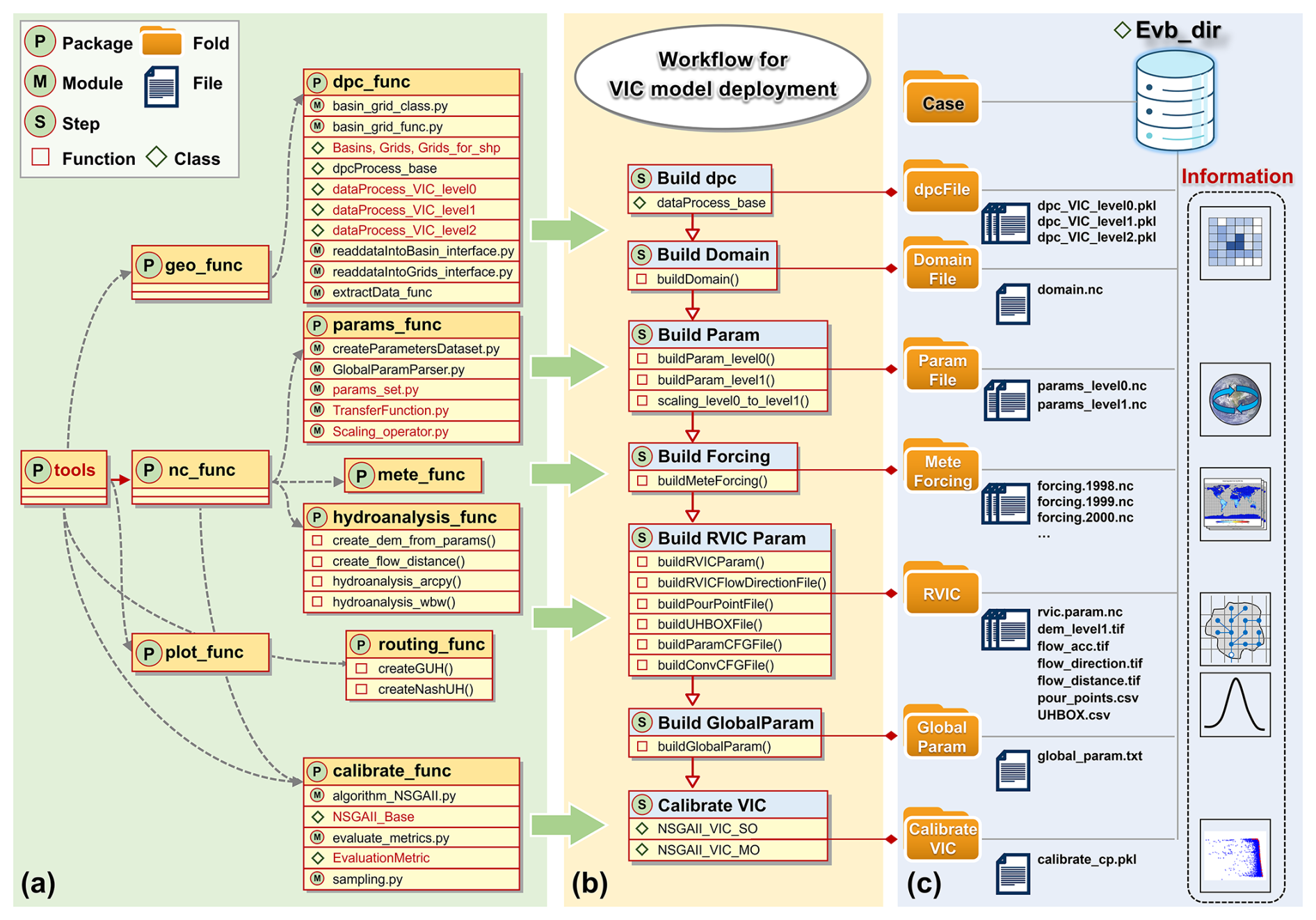
Figure 1 The architecture of the Easy VIC Build (EVB) framework. (a) The tools subpackage, along with its structure, forms the essential foundation that underpins the functionality and operation of other modules. (b) The workflow for VIC model deployment and related modules. (c) The file tree structure generated by the EVB framework, which is managed by the Evb_dir class, contains the information for the deployment of the VIC model. The core modules or classes are marked in red.

Here, we highlight the advantages of this architectural design, specifically its object-oriented programming and loosely coupled structure. This is achieved by decomposing various functionalities into separate classes, functions, modules, and subpackages, allowing the users to modify and extend the framework as needed at any time. For example, the addition of a new forcing data source can be accommodated by overriding the relevant methods of the data processing class, without modifying other components. These design choices are consistent with the principles of reproducibility, grouping, isolation, and sharing highlighted by Hamman et al. (2018) and Knoben et al. (2022). Below, we introduce several classes that constitute the core of the EVB architecture, along with the underlying concepts.

2.1.1 Two fundamental classes for geographic information: Grids and Basins

Each deployed hydrological model is intrinsically linked to a specific region (or basin) and a corresponding horizontal discretization, both of which embed spatial information that can be mapped to other information, such as soil properties. Typically, the region is represented by a shapefile within a GIS, either supplied by the user or derived through a relevant basin delineation method. Meanwhile, horizontal discretization is commonly achieved using a structured array of rectangular grids.

To enable an object-oriented representation within this framework, we constructed two subclasses, termed Basins and Grids, which inherit from the GeoDataFrame class provided by the GeoPandas package (Jordahl et al., 2020). In this way, they inherit the advantages and functionality of their parent class, such as convenient plotting and I/O (i.e., input and output) capabilities. These two subclasses provide a unified representation of the two types of geographic information mentioned above, and they act as proxies for regions and grids while sharing their geographic information throughout the model deployment workflow. From an architectural design perspective, they serve as the foundation for data processing classes (hereafter dpc classes), thereby enabling interfaces for interaction with other information or data.

2.1.2 Information level division of modelling scale and the data processing classes

A hydrological model is an integration of information from multiple scales. For the VIC model, information from both finer scales (e.g., land surface information at the kilometer level) and coarser scales (e.g., meteorological forcing information at tens-of-kilometers level) must be unified to a predefined, singular modelling scale. It is essential for modelers to clearly distinguish between the scales of different information. Here, we adopt the concept proposed by Samaniego et al. (2010), who divided the spatial scales into three levels: level-0, level-1, and level-2. In brief, information at level-0 is used to describe sub-grid variability of basin characteristics at finer scales, such as topography and soil properties. Level-1 is associated with the modelling scale and represents the scale at which the primary hydrological processes are focused. Finally, level-2 corresponds to the meteorological forcing scale. Here, we further introduce a level-3 representation to capture basin scale information, such as watershed characteristics and outlet runoff. This multiscale classification facilitates the integration of information across different spatial scales and provides a basis for implementing the Multiscale Parameter Regionalization (MPR) technique. Building on the information level division, we established an abstract base class for data processing and subsequently implemented several VIC-specific subclasses, collectively refer to as dpc classes (Fig. 1a). They share a similar structure but encompass different information at diverse scales. Each dpc class contains a Basins and a Grids instance as attributes to represent geographic information at their respective scale.

2.2 Environmental requirements

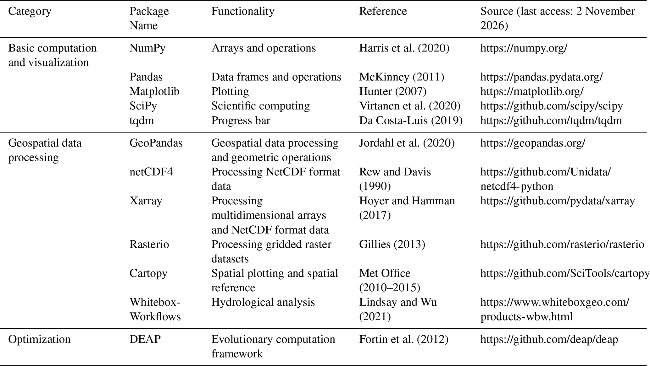
The EVB framework is fully developed in Python and entails certain basic environmental requirements. All the required environments are open-source and easily accessible. To assist users in configuration, we grouped the required environments into three categories based on their functionality: (a) basic computation and visualization, (b) geospatial data processing, and (c) optimization. Table 1 lists the names and sources of these Python packages. We also provide a pyproject.toml file in the source code, aligned with the latest Python standards, to simplify the environment setup.

Table 1 A summary of the EVB framework environmental requirements.

3 Functionalities of the EVB

To make this study self-contained and easy to follow, basic descriptions, where necessary, of the functionalities of the EVB are provided in this section. Prior to describing the workflow of VIC deployment in the EVB, it is important to first introduce two related techniques.

3.1 Multiscale Parameter Regionalization technique

The Multiscale Parameter Regionalization (MPR) technique was pioneered by Samaniego et al. (2010), with the aim of proposing a method for the parameter estimation of distributed hydrological models at multiple scales. A distinctive feature of MPR is the combination of the transfer function and scaling operator. Following the information level division approach described earlier, at level-0, basin characteristics such as soil properties are transferred into effective parameters via the transfer function, after which the scaling operator is applied to scale these parameters to level-1. During this process, a set of spatially invariant, quasi-scale independent, scalar global parameters is used (hereafter referred to as g-parameters), making calibration possible and enhancing its applicability.

Notably, the feasible ranges of the g-parameters are constrained based on previous transfer-function studies, ensuring physically meaningful parameter bounds rather than arbitrary assignments. For example, according to the work of Cosby et al. (1984), the relationship between saturated hydraulic conductivity (K_S) and soil texture can be expressed as follows:

$$\begin{array}{}\text{(1)}& \log K_{\mathrm{s}}=\mathrm{0.0126}{f}_{\text{sand}}-\mathrm{0.0064}{f}_{\text{clay}}-\mathrm{0.6},\end{array}$$

where f_sand denotes the sand content fraction and f_clay denotes the clay content fraction. Using this empirical relationship as prior knowledge, a transfer function incorporating the g-parameters can be established, allowing K_S to be inferred from soil texture:

$$\begin{array}{}\text{(2)}& K_{\mathrm{s}}={\mathrm{10}}^{g_{\mathrm{1}}+g_{\mathrm{2}}{f}_{\text{sand}}+g_{\mathrm{3}}{f}_{\text{clay}}},\end{array}$$

where g represents the g-parameters, and their feasible ranges (Table A1) can be obtained by proportionally scaling the coefficients from the original equation. Here, g₁, g₂, and g₃ correspond to g₆, g₇, and g₈ in Table A1, respectively.

Additionally, we extended the transfer functions to include parameters of the routing-module. Specifically, the flow velocity and diffusion coefficient were regionalized based on grid-level river network information using mapping relationships reported in previous studies (Chen et al., 2019; Yang et al., 2016), resulting in spatially distributed parameter fields as formulated below:

$$\begin{array}{}\text{(3)}& {\displaystyle }v=g_{\mathrm{1}}{\text{acc}}^{g\mathrm{2}}{S}^{g\mathrm{3}},\text{(4)}& {\displaystyle }D=g_{\mathrm{4}}dv,\end{array}$$

where acc is the accumulated upstream area, and S denotes the mean slope angle, d is the flow distance within each grid.

The MPR technique has been successfully applied to parameter estimation in various distribution hydrological models, including but not limited to the VIC and mHM models (Rakovec et al., 2016; Zink et al., 2017). All these studies have consistently demonstrated that the parameters estimated by MPR exhibit a certain degree of transferability. A recent study by Mizukami et al. (2017) is an important starting point for this study. They implemented the MPR technique for the VIC model using Fortran and generated parameter estimates for a large sample of basins across the CONUS. The EVB framework proposed here partially builds upon the transfer functions they used, with one improvement being its implementation in Python and in a modular, object-oriented manner rather than the original Fortran functional programming approach. The transfer functions used for the VIC model-specific parameterization in this study are detailed in Table A2 in the Appendix.

Within the EVB framework, the MPR method serves as a core module for VIC parameter estimation during the model deployment process. It offers the following advantages: (1) a user-friendly parameter estimation approach, with all parameter-related knowledge aggregated within the transfer function; (2) some extent of parameter transferability across scales and regions; and (3) the consideration of the influence of basin characteristics on parameters, making them more physically meaningful.

3.2 General Unit Hydrograph technique

The Unit Hydrograph (UH) concept is a classical concept in hydrology, first introduced by Sherman (1932). Fundamentally, the rainfall–streamflow transformation is represented using a convolution-based transfer function model (TFM). Owing to its simple structure and computational efficiency, it can serve as an effective black-box routing approach. The RVIC routing model integrated within the VIC source code is a variant of the UH (Lohmann et al., 1996), which requires a grid UH for its parameter derivation.

Over the past decades, various forms of UH have been developed, such as the Nash UH based on a two-parameter Gamma distribution and the Soil Conservation Service (SCS) dimensionless UH. Among these forms, a General UH (GUH) introduced by Guo (2022) has a particular appeal as it has explicit analytical expressions:

$$\begin{array}{}\text{(5)}& {\displaystyle }u\left(t\right)={\displaystyle \frac{\mathrm{d}g}{\mathrm{d}t}}={\displaystyle \frac{\mathit{\mu }}{t_{\mathrm{p}}}}x(\mathrm{1}+mx{)}^{-(\mathrm{1}+\mathrm{1}/m)},\text{(6)}& {\displaystyle }g\left(t\right)=\mathrm{1}-(\mathrm{1}+mx{)}^{-\mathrm{1}/m},\text{(7)}& {\displaystyle }x\left(t\right)=\exp \left[\left(\mathit{\mu }\left({\displaystyle \frac{t}{t_{\mathrm{p}}}}-\mathrm{1}\right)\right)\right],\end{array}$$

where t_p is the peak flow time; m is a dimensionless recessing coefficient determined by downstream water surface conditions; and μ is the rising coefficient related to the basin characteristics. This analytical expression provides high flexibility to the GUH and has been demonstrated to exhibit high consistency with traditional methods (Guo, 2022). In this study, the GUH is employed as the default grid UH to derive the RVIC parameters. Its shape is controlled by the above three parameters, which are treated as free parameters to be calibrated. To enhance flexibility and user configurability, the Nash UH is also implemented as an optional alternative.

3.3 Workflow for VIC model deployment

Figure 1b presents the VIC model deployment workflow within the EVB framework, which consist of seven sequential steps. This deployment process follows the guidelines outlined in the official VIC documentation (https://vic.readthedocs.io/, last access: 2 November 2026) and focuses on the image driver version of VIC-5. The workflow is described in detail below, with all files involved in the deployment process managed through EVB's built-in Evb_dir class. This class provides unified path management for the definition, modification, and transfer of file and directory paths, thereby ensuring consistent and efficient file handling throughout the deployment.

The workflow first processes the required spatial and attribute data according to the selected modelling domain and spatial discretization. Users construct Grids and Basins instances and provide them to the corresponding dpc instances, where data source-specific extraction and processing are performed. The resulting basin- and grid-level information is stored as instance attributes for subsequent deployment steps. Based on the processed level-1 data, the build_Domain utility then generates the VIC domain file in NetCDF format, including grid area, basin fraction, and grid-edge information.

VIC parameter files are subsequently generated using the MPR-based parameterization scheme embedded in EVB. The scheme maps level-0 basin characteristics to spatially distributed parameters at the selected modelling scale, while the g-parameters can be calibrated to account for basin-specific conditions. Meteorological forcing is generated from the processed dpc instances using the buildMeteForcing function. The required VIC forcing variables are prepared and converted when necessary, for example, deriving vapor pressure from specific humidity and wind speed from its zonal and meridional components. The resulting forcing files are stored in NetCDF format and can be directly used by VIC.

For runoff routing, EVB uses the Python implementation of RVIC to generate routing parameter files. This procedure first derives the hydrological topology from the level-1 DEM and then generates the required routing inputs, including the pour point and unit hydrograph. Users can select either the Nash or GUH unit hydrograph, while flow velocity and diffusion parameters can be regionalized using the MPR scheme and calibrated when required. A global parameter file is finally generated and managed through the GlobalParamParser, which facilitates the specification and modification of model input/output paths and runtime options.

The final step is VIC model calibration. Although MPR provides spatially distributed parameter estimates, calibration remains necessary to account for uncertainties in regionalized parameters and their scaling across spatial resolutions. EVB provides both the Covariance Matrix Adaptation Evolution Strategy (CMA-ES; Hansen and Ostermeier, 2001) and the Non-dominated Sorting Genetic Algorithm II (NSGA-II; Deb et al., 2002) through the DEAP library for single- and multi-objective calibration, respectively, allowing users to calibrate selected model parameters against streamflow and, where available, additional hydrological observations.

4 Case basins and data collection

To illustrate the efficacy of the EVB framework in facilitating the flexible deployment of the VIC model, we designed two basin setups, each representing a typical research scenario. The former exemplifies the increasingly popular large-sample basin research paradigm (Yeste et al., 2024), whereas the latter corresponds to the more traditional site-specific approach in hydrological studies. Then, these two basin setups were used as test cases to assess the performance and efficiency of the EVB-VIC modelling framework across multiple hydrological applications. The subsequent section delineates the basin setups and the requisite data for model implementation.

4.1 Basin setup A: case basin from large-sample dataset

In response to the call for large-sample hydrological research highlighted by Gupta et al. (2014), we assess whether the EVB framework can contribute to this research direction. To this end, we selected a case basin from the widely used Catchment Attributes and Meteorology for Large-sample Studies (CAMELS) dataset (Newman et al., 2015; Addor et al., 2017) to demonstrate the implementation of VIC modelling within the EVB framework. Employing a simple model setup with streamflow-only calibration, we investigated the parameter transferability to evaluate the efficiency of applying EVB in large-sample basin contexts. The case basin is located within Missouri, USA, and is known as the Gasconade River Basin (GRB; USGS gauge ID: 06934000), with a total drainage area of approximately 8268 km². Figure 2 provides an illustrative map of the basin, showcasing the topography, outlet, and land surface properties in the area. The local temperate continental climate is typical and characterized by distinct seasonal variations. Under the combined effects of climate, topography, and vegetation, streamflow in this area exhibits pronounced seasonal variability, with the peak flow occurring in the spring and a low flow observed in the late summer and autumn. Notably, the current EVB implementation, once demonstrated in this case basin, can be seamlessly extended to the entire CAMELS basin collection.

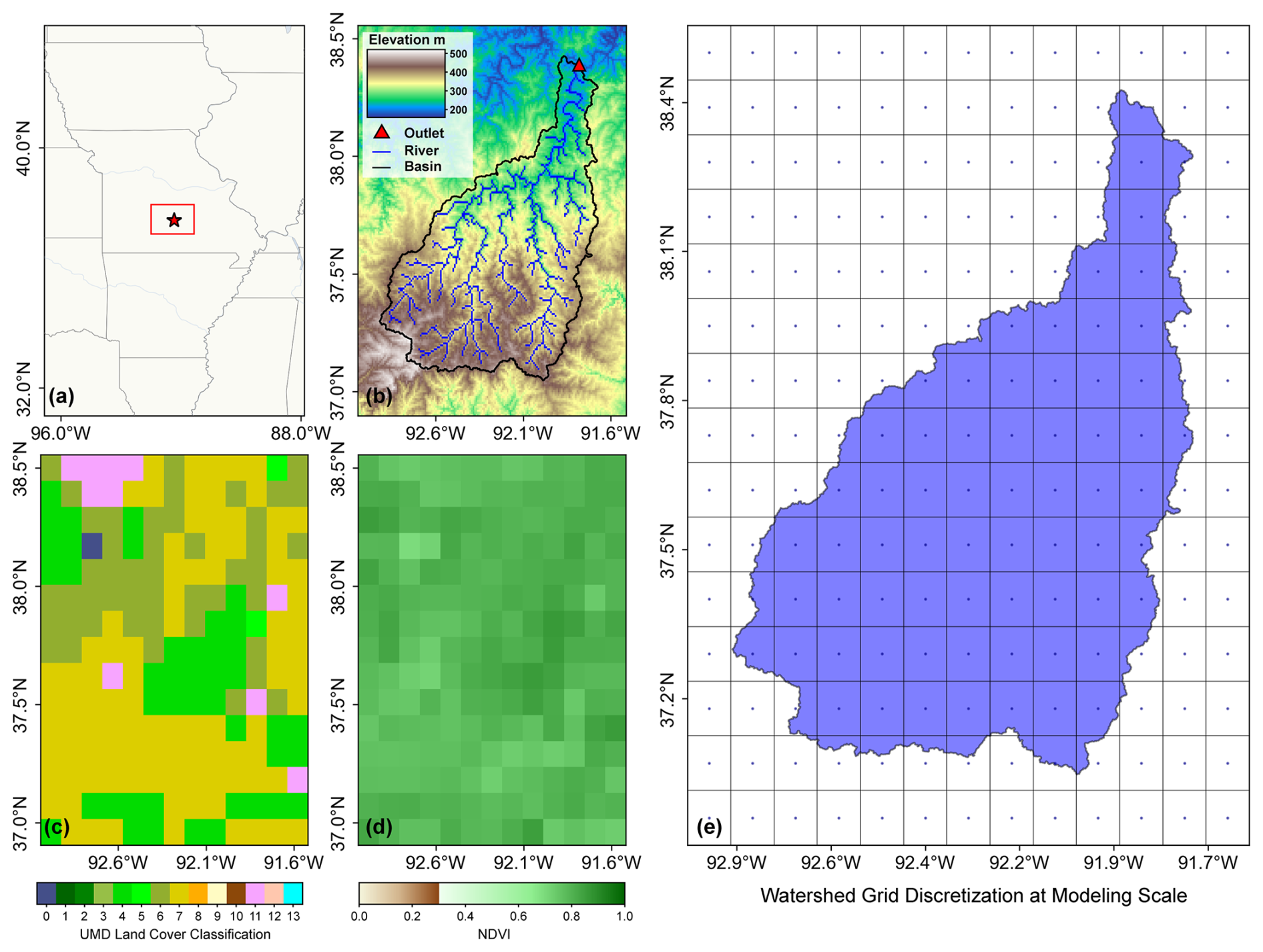
Figure 2 Overview of the Gasconade River Basin. (a) Location within Missouri, USA. (b) Topography, river network, and outlet location. (c) Dominant land cover classes according to the University of Maryland Global Land Cover dataset (Hansen et al., 2021). (d) Averaged NDVI from the MOD13A3.061 dataset (Didan, 2021). (e) Watershed grid discretization at modelling scale (i.e., 12 km×12 km).

4.2 Basin setup B: single site-specific basin

Beyond large-sample applications, we further assess the adaptability of the EVB to the single site-specific basin setup, a typical case in which researchers define or customize their own study domain. Within this setup, a more complex multi-objective calibration was employed, alongside an in-depth examination of the physical plausibility of the spatial parameter distributions. Here, we selected the Jing River Basin (hereafter referred to as JRB), with a drainage area of approximately 45 400 km², as the case basin. It represents a markedly different hydroclimatic setting compared to GRB, characterized by a typical arid to semi-arid climate and land use condition representative of northern China (Fig. 3).

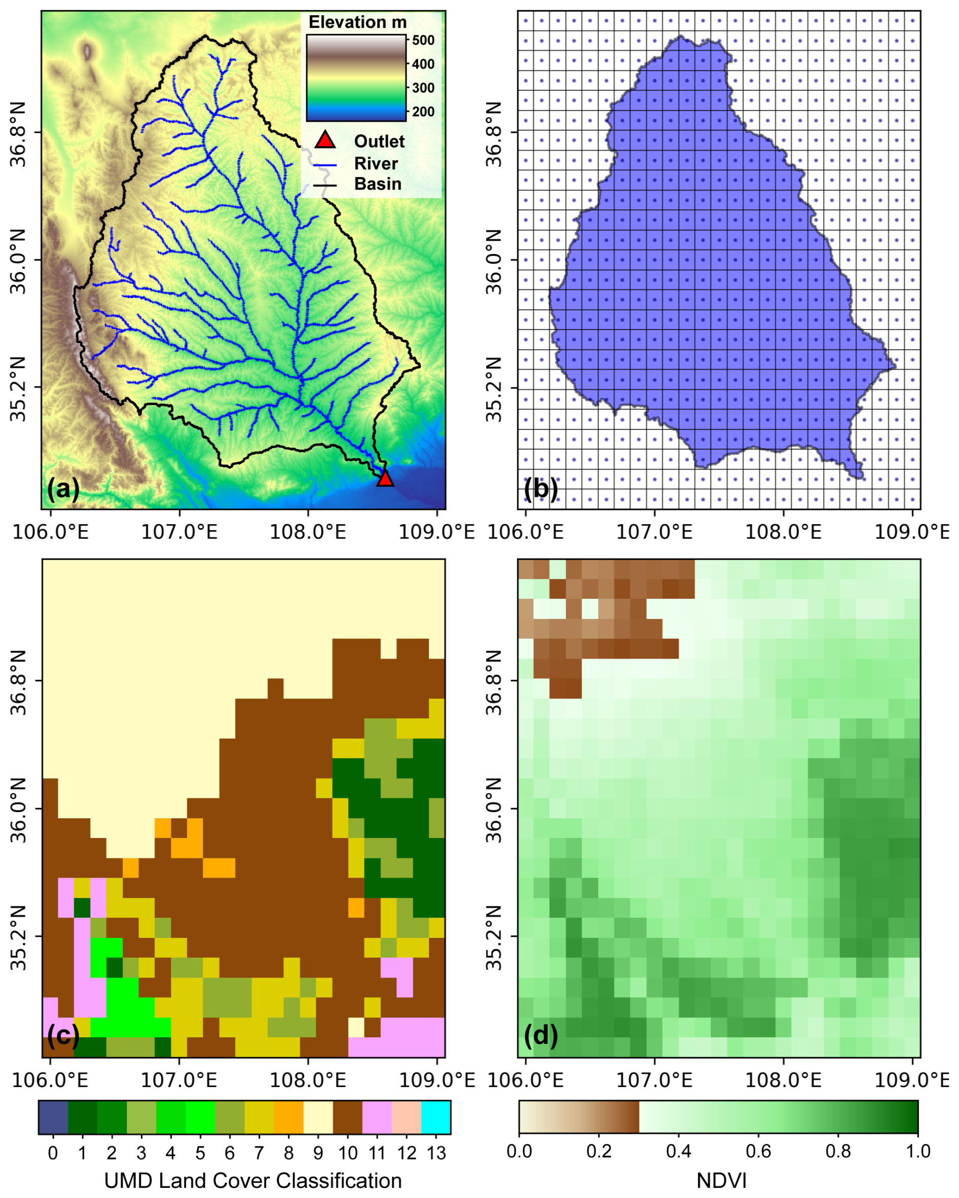
Figure 3 Overview of the Jing River Basin. (a) Topography, river network, and outlet location. (b) Watershed grid discretization at modelling scale (i.e., 13.8 km×13.8 km). (c) Dominant land cover classes according to the University of Maryland Global Land Cover dataset (Hansen et al., 2021). (d) Averaged NDVI from the MOD13A3.061 dataset (Didan, 2021).

4.3 Data collection

4.3.1 Datasets used in basin setup A

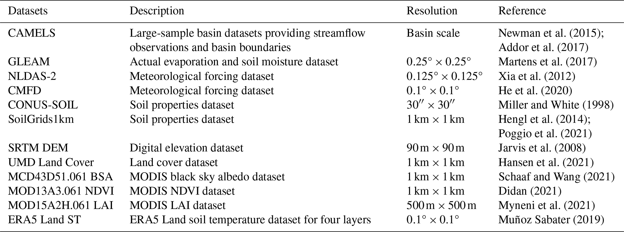
The extracted information on daily streamflow, basin boundaries, and outlet location of GRB from the CAMELS dataset provides essential input for deploying the VIC model. Other distributed data are also required. First, the hourly forcing, including precipitation, downward longwave radiation, downward shortwave radiation, surface pressure, specific humidity, air temperature, and wind speed, was acquired from Phase 2 of the North American Land Data Assimilation System (NLDAS-2) forcing dataset with a spatial resolution of 0.125° and covering the period from 1998 to 2010 (Xia et al., 2012). This dataset was originally developed to force several LSMs, including VIC, and it is derived from the analysis fields of NCEP North American Regional Reanalysis (NARR). It has been validated in a range of hydrological modelling studies, demonstrating robust applicability (Sun et al., 2021; Yan et al., 2023).

Second, several datasets were collected to describe the static features of the underlying surface (i.e., soil, topography, land cover type, and vegetation). Specifically, the soil texture (i.e., the proportions of sand, loam, and clay) and the bulk density of 11 soil layers (ranging from 0 to 2.5 m in depth) were obtained from the conterminous United States (CONUS-SOIL) dataset (Miller and White, 1998). The data from the Shuttle Radar Topography Mission (SRTM) Digital Elevation Model (DEM) V4.1 (90 m) were used to describe the topography (Jarvis et al., 2008). The 1 km gridded global land cover dataset from the University of Maryland (UMD Land Cover) provides information on 14 land cover classes (Hansen et al., 2021). Vegetation information includes monthly data on the partial vegetation cover fraction (fcanopy), the leaf area index (LAI), and the albedo. Following previous studies, the fcanopy can be derived from the Normalized Difference Vegetation Index (NDVI) using the following formula (Bohn and Vivoni, 2019):

$$\begin{array}{}\text{(8)}& f_{\text{canopy}}={\left({\displaystyle \frac{\text{NDVI}-{\text{NDVI}}_{\text{min}}}{{\text{NDVI}}_{\text{max}}-{\text{NDVI}}_{\text{min}}}}\right)}^{\mathrm{2}}.\end{array}$$

On this basis, multi-year data for albedo, NDVI, and LAI were extracted from several derived Moderate Resolution Imaging Spectroradiometer (MODIS) products (MCD43D51.061, MOD13A3.061, and MOD15A2H.061) and mosaicked into monthly values. Finally, the four-layer soil temperature from the ERA5 Land product is extracted and averaged to serve as the bottom boundary condition for the soil heat flux in the VIC model.

4.3.2 Datasets used in basin setup B

For site-specific VIC modelling application, we incorporated additional datasets applicable to the JRB, alongside the aforementioned global datasets. These include SoilGrids1km for detailed soil property information (Hengl et al., 2014; Poggio et al., 2021) and the China Meteorological Forcing Dataset (CMFD) for localized meteorological forcing (He et al., 2020). The latter provides high spatiotemporal resolution (0.1°, 3 hourly) data for seven essential variables across China, making it well-suited for constructing meteorological forcing inputs required by the VIC hydrological model in JRB.

As mentioned above, we considered different complementary objectives during the calibration process. On the one hand, we evaluated the model's ability to reproduce the temporal dynamics of streamflow by comparing the simulated results with in situ observations from the Zhangjiashan hydrological station (108.60° E, 34.63° N; Fig. 3a). On the other hand, we assessed its capability to capture the patterns of actual evaporation and soil moisture. The reference data of these two variables were obtained from the Global Land Evaporation Amsterdam Model (GLEAM) dataset (Martens et al., 2017). Since the GLEAM dataset employs a conceptual water balance soil module, the surface (0–10 cm) and root-zone (10–100 cm) soil moisture were aggregated to estimate total soil moisture, so as to allow a comparison with the VIC model outputs. In this context, analyzing the patterns consistency between the simulated and reference data proves more meaningful than direct magnitude comparisons.

The datasets listed above are publicly available and widely used in hydrological modelling. An overview of these datasets is provided in Table 2.

Table 2 An overview of the datasets used for deploying the VIC model.

5 Modelling Applications based on the EVB

5.1 VIC Model deployment

The VIC model instances were deployed via the EVB framework at multiple spatial resolutions (i.e., 6, 8, and 12 km) in basin setup A, and at a fixed resolution (i.e., 13.8 km) in basin setup B. The spatial resolutions of level-0 and level-2 are determined based on the data availability and are set to 1 km and 0.125°, respectively. The data listed in Table 2 were resampled to the corresponding spatial resolutions, and the input files required for running VIC were generated following the deployment workflow described above.

To provide a full narrative of the VIC deployment, there are two configurations that need to be clarified – data partitioning and parameter calibration. For basin setup A, the period from 1998 to 1999 served as a warm-up period to ensure stable initial conditions. The model was then calibrated using daily streamflow records from 2000 to 2007 to derive the optimal parameter set, with the remaining 3 years reserved for validation. For the objective function, we use the KGE metric on streamflow, which is a widely recognized measure of model performance that integrates bias, variance, and correlation (Gupta et al., 2009). Further evaluation metrics, including NSE and PBIAS, are employed to comprehensively evaluate model performance during the validation period (Mizukami et al., 2019). Formally, these metrics can be calculated using the following formulas:

$$\begin{array}{}\text{(9)}& {\displaystyle }\text{KGE}=\mathrm{1}-\sqrt{(r-\mathrm{1}{)}^{\mathrm{2}}+{\left({\displaystyle \frac{{\mathit{\sigma }}_{\text{sim}}}{{\mathit{\sigma }}_{\text{obs}}}}-\mathrm{1}\right)}^{\mathrm{2}}+{\left({\displaystyle \frac{{\mathit{\mu }}_{\text{sim}}}{{\mathit{\mu }}_{\text{obs}}}}-\mathrm{1}\right)}^{\mathrm{2}}},\text{(10)}& {\displaystyle }\text{NSE}=\mathrm{1}-{\displaystyle \frac{{\sum }_{i=\mathrm{1}}^n(V_{\text{obs}}^i-V_{\text{sim}}^i{)}^{\mathrm{2}}}{{\sum }_{i=\mathrm{1}}^n(V_{\text{obs}}^i-\stackrel{\mathrm{‾}}{V_{\text{obs}}}{)}^{\mathrm{2}}}},\text{(11)}& {\displaystyle }\text{PBIAS}={\displaystyle \frac{{\sum }_{i=\mathrm{1}}^n(V_{\text{obs}}^i-V_{\text{sim}}^i)}{{\sum }_{i=\mathrm{1}}^n{V}_{\text{obs}}^i}}\times \mathrm{100}\mathit{\%},\end{array}$$

where σ is the standard deviation; and μ is the mean; Vⁱ is the target variable (i.e., streamflow) at time step i; and n is the length of the sequence. The subscripts sim and obs denote the simulated and observed values. Both KGE and NSE are formulated such that higher values indicate better model performance, with a value of 1 representing the optimal simulation for each metric. The final metric, PBIAS, is used to evaluate whether the model overestimates (PBIAS<0) or underestimates (PBIAS>0) the observed values.

In the case of basin setup B, the years 2008–2009 were allocated for model warm-up, 2010–2015 for calibration, and 2016–2018 for validation. A special setting in this setup is that multiple objective functions were formulated to improve the simulation performance with respect to various aspects of the VIC model during the calibration process. Besides using KGE to evaluate streamflow and actual evaporation simulation, the model capability to reproduce the patterns of soil moisture was assessed via the Pearson correlation coefficient (R), which is formulated as follows (Wambura et al., 2018):

$$\begin{array}{}\text{(12)}& R={\displaystyle \frac{{\sum }_{i=\mathrm{1}}^n(V_{\text{obs}}^i-\stackrel{\mathrm{‾}}{V_{\text{obs}}})(V_{\text{sim}}^i-\stackrel{\mathrm{‾}}{V_{\text{sim}}})}{\sqrt{{\sum }_{i=\mathrm{1}}^n(V_{\text{obs}}^i-\stackrel{\mathrm{‾}}{V_{\text{obs}}}{)}^{\mathrm{2}}}\sqrt{{\sum }_{i=\mathrm{1}}^n(V_{\text{sim}}^i-\stackrel{\mathrm{‾}}{V_{\text{sim}}}{)}^{\mathrm{2}}}}},\end{array}$$

where Vⁱ is the target variable at time step i and the overbar indicates the average.

Both basin setups used a two-year warm-up period to allow the model states, particularly soil moisture, to reach stable initial conditions. This period length was guided by previous studies and established modelling practice. For example, Miao and Wang (2020) found that soil moisture at nine representative grid cells had largely reached equilibrium after two years when developing a VIC based land surface hydrological dataset for China. Several other studies have likewise used warm-up periods of one to three years (Nicolle et al., 2014; Qiu et al., 2017; Mei et al., 2023). Drawing on this evidence and considering data availability, we selected a two-year warm-up period to maintain a practical balance among the warm-up, calibration, and validation periods. Simulated runoff remained relatively stable during the early part of the subsequent simulation period, with no pronounced extreme values, further supporting this choice.

In this study, parameter calibration was performed using the CMA-ES and NSGA-II algorithm implemented in the EVB, as described in Sect. 3.3. The CMA-ES algorithm is configured with a population size of 40, and the initial global step size (σ) is set to 0.4. The NSGA-II algorithm is configured with a population size of 20, a crossover probability of 0.7, and a mutation probability of 0.2. Polynomial mutation and simulated crossover are employed. To mitigate potential identifiability issues arising from a large number of free parameters, we fixed some of the physical parameters and introduced a simplified calibration set, reducing the free parameters from 44 to 15. A substantial body of research (Liang et al., 1994; Gou et al., 2020; Gu et al., 2021; Cortés-Salazar et al., 2023; Yeste et al., 2024), together with widespread VIC modelling practice, supports the selection of this reduced parameter set as comprising parameters commonly identified as sensitive. All 15 free parameters (Table A3) are treated equivalently within a parameter pool and sampled by Latin hypercube sampling (LHS) to partition the parameter space into equiprobable regions with representative samples, thereby ensuring efficient coverage of entire parameter range (McKay et al., 1979).

The optimization was performed for a maximum of 200 generations and stopped upon convergence, with the optimal parameters selected according to the maximum KGE in basin setup A. For the multi-objective calibration in basin setup B, a best Pareto front comprising multiple non-dominated optimal solutions was generated, from which a solution exhibiting a relatively balanced trade-off among objectives was manually selected as the final parameter set. The convergence process of the single-objective calibration and the Pareto front curves from the multi-objective calibration are provided in Figs. B1 and B2, respectively.

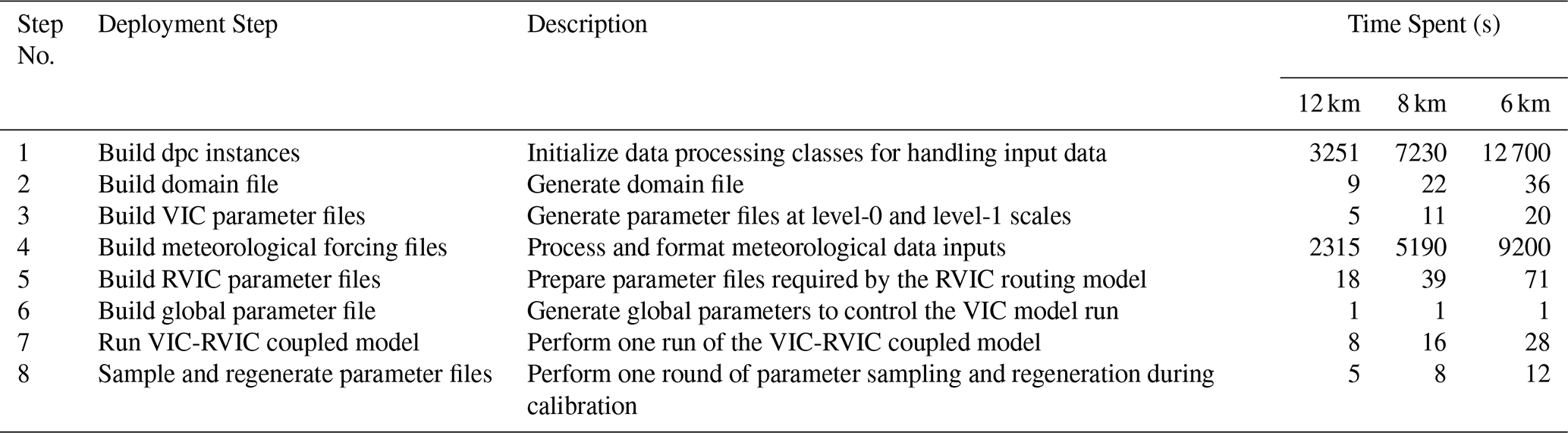
Noteworthily, all experiments in this study were performed on a laptop with 32.0 GB of RAM, with an AMD Ryzen 7 8845H 3.80 GHz processor, and running Ubuntu 20.04.1 LTS (virtual machine). To illustrate the computational efficiency of EVB, we used the built-in Logger class to record the average time required for each deployment step across the three spatial resolutions considered in the first case application (i.e., GRB), as described later; the results are reported in Table 3. The Logger class automatically records the execution time of each step and generates messages at predefined logging levels, providing traceability throughout the model deployment process. Building dpc instances (57 % of the total runtime) and processing meteorological forcing data (41 %) are the primary time-consuming steps, but both need to be executed only once for each modelling application and can thereafter be saved to persistent storage for convenient reuse. Because these operations are performed on a grid-cell basis, their computational costs increase approximately linearly with the number of grid cells as the spatial resolution becomes finer.

Table 3 Time consumption for EVB deployment workflow.

5.2 Modelling application in basin setup A

5.2.1 Parameter transferability across different spatial scales

Proceeding from the simplest case, we examined the capability of the coarsest-resolution (i.e., 12 km) VIC configuration to simulate daily streamflow. As shown in Fig. 4, the seasonal and event-based variations in streamflow are generally well reproduced, although some fluctuations remain in the simulated time series. The evaluation metrics also indicate a satisfactory performance, with KGE, NSE, and PBIAS values of 0.60 %, 0.61 %, and −28.67 % for the calibration period. The corresponding values for the validation period (0.60 %, 0.63 %, and −5.92 %) indicate no substantial degradation in performance. We further evaluated model performance separately for low-flow (<30th percentile) and high-flow (>70th percentile) regimes, defined based on the total streamflow range. In this way, a consistent pattern in model behaviour emerged across different periods, dominated by a pronounced overestimation during low-flow conditions and a slight underestimation during high-flow conditions (right panels in Fig. 4). Such behaviour was also appreciated in the detailed analyses of previous studies (Wenger et al., 2010; Lehmann et al., 2022). Overall, the above analysis indicates that the streamflow simulation performance is acceptable.

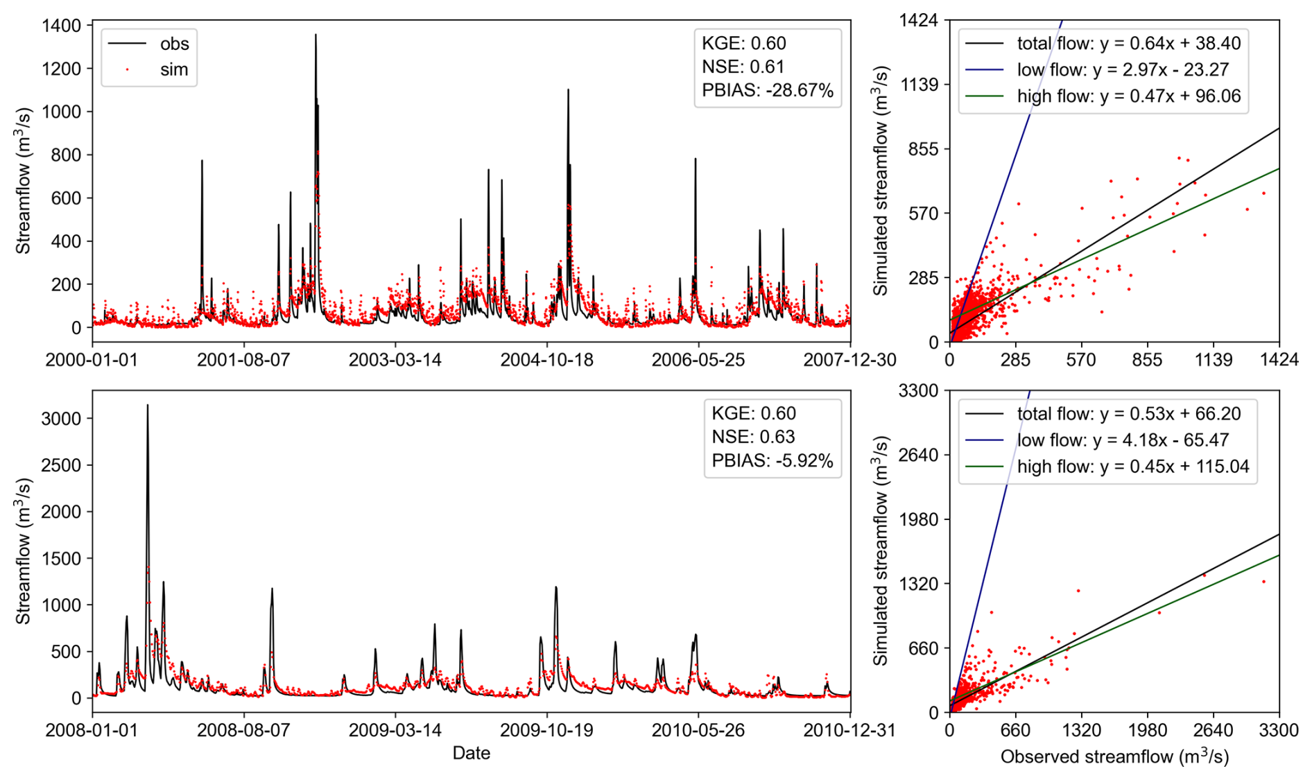
Figure 4 Comparison of daily simulated streamflow from the 12 km-resolution VIC model against observations during the calibration period (top two panels) and validation period (bottom two panel). Low-flow and high-flow thresholds are defined as 30th and 70th percentiles of the total flow range, respectively.

We next evaluate the transferability of parameters across spatial scales – a key feature of EVB's deployment potential to support VIC applications under different spatial configurations. To this end, the 15-parameter set calibrated at 12 km resolution was transferred to 6 and 8 km models (hereafter denoted as VIC-6, VIC-8, and VIC-12). The resulting simulations were then compared to access parameter transferability. Figure 5 provides an intuitive comparison of model performance in streamflow simulation through Taylor diagram analysis. Both panels of the figure suggest that parameters transfer from a coarser resolution (12 km) to finer resolutions (6 and 8 km) preserves model performance, as evidenced by the close clustering of three points in Taylor diagram space. Figures C1 and C2 present the simulated hydrographs and corresponding evaluation metrics for the VIC-8 and VIC-6 models. Although calibration-period performance of transferred models declined relative to VIC-12, it remained within acceptable thresholds (KGE>0.50, NSE>0.58). Importantly, no degradation occurred during the validation period, with both KGE and NSE of transferred models exceeding 0.62. Such parameter transferability was achieved through the MPR technique, which links different spatial scales using the same underlying input data at level-0 and the corresponding transferred g-parameters.

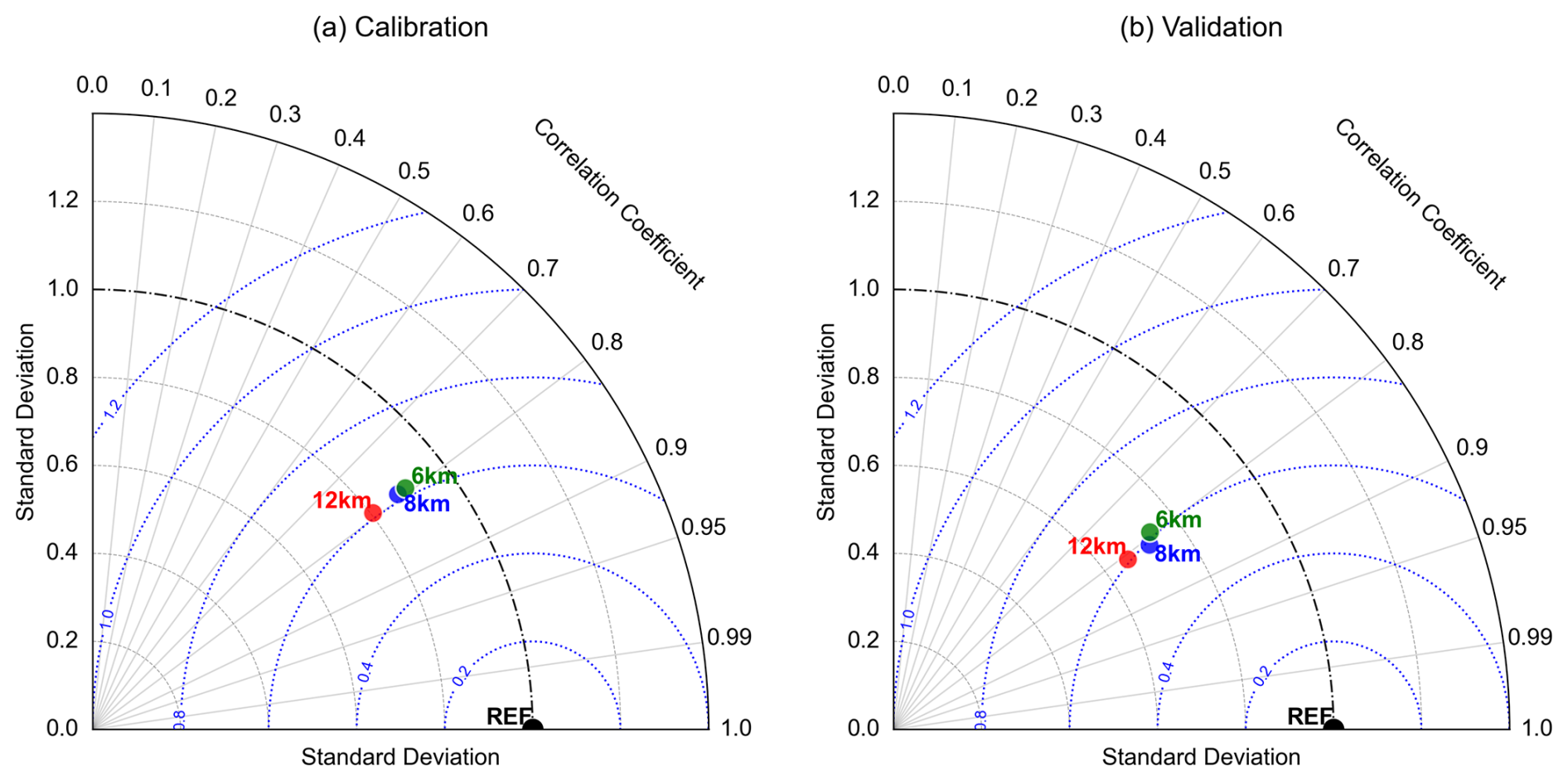
Figure 5 Taylor diagrams of daily simulated streamflow from the VIC model at three spatial scales (6, 8, and 12 km). Both simulated and observed values are standardized, with the observed values (REF point) having a standard deviation of 1.0. Blue dashed contours indicate root mean square error (RMSE) relative to observed benchmarks.

5.2.2 Distributed simulations of surface runoff and baseflow

Surface runoff and baseflow are recognized as the dominant hydrological components governing high-flow and low-flow conditions, respectively, and are often conceptualized as rapid response and slow response processes within watershed systems (Liu et al., 2012a; Singh et al., 2018). From this perspective, the analysis presented in the preceding section raised a critical question: given that the model has demonstrated scale transferability in hydrograph simulation, does it also reproduce consistent spatial distributions of runoff generation processes across different scales? To address this issue, we selected a representative single-peak flood event spanning the period of 1 February 2001 to 31 March 2001, to examine the runoff generation processes across varying scales. Specifically, we focus on the distributed simulations of particular components – namely, the surface runoff during the rising period and the baseflow during the recession period.

The event-based simulation results are presented in Fig. 6, showcasing the streamflow hydrographs alongside the spatial distribution of the two runoff components. A clear observation is that the three simulated hydrographs exhibit remarkable consistency. The spatial distribution of surface runoff during the rising phase illustrates the runoff generation processes, peaking on 24 February, coinciding with the timing of the peak rainfall (Fig. 6b), while the routed flow took approximately two days to reach the hydrograph peak at the outlet (Fig. 6a). This pattern is consistent across resolutions without significant magnitude variations. In terms of the distributed simulation of baseflow, all models consistently produced only a minor decrease in the central part of the basin during the recession period. This indicates that the model interprets this flood event as primarily dominated by surface runoff, whereas baseflow maintaining the multi-year baseline discharge in the river channel. Another finding from Fig. 6 is the pronounced underestimation of peak flows, which our analysis suggests stems from inadequate surface runoff generation. This could potentially be improved in future calibrations by including peak-flow-focused signature metrics in the objective function (Mizukami et al., 2019).

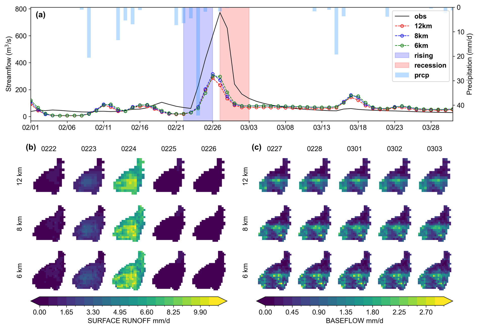
Figure 6 Scatterplots of daily simulated streamflow from the VIC model at three spatial scales (6, 8, and 12 km) against observations. The total sample is partitioned into low-flow and high-flow subsets for comparative evaluation, with the thresholds set at the 30th and 70th percentiles of the total flow range.

5.3 Modelling application in basin setup B

5.3.1 Multi-objective simulation performance

Relying solely on single-objective calibration using outlet streamflow is increasingly considered insufficient to address the growing demands of the hydrological modelling community (Beven, 2024). To support the goal of producing the right results for the right reasons and to improve model credibility, it is essential to integrate multiple data sources into the calibration process. In this section, we explore this potential application in the JRB basin.

Figure 7 shows the VIC simulation results obtained with the optimal parameter set derived from a three-objective calibration against streamflow, actual evaporation, and soil moisture. It can be seen that streamflow performance is acceptable in both the calibration and validation periods, with KGE exceeding 0.7 and absolute PBIAS below 3 %, indicating good simulation of total streamflow. However, NSE values below 0.5 indicate that the VIC model performs relatively poorly in capturing peak flows in the JRB basin, as NSE is particularly sensitive to high flows (Mizukami et al., 2019; Zhong et al., 2023). Such behaviour has been documented in earlier VIC modelling studies, especially for arid basins similar to the JRB (Gou et al., 2020; Lehmann et al., 2022). In terms of evaporation, the VIC model reproduces the seasonal variation pattern well (KGE>0.8), but it tends to overestimate certain summer peaks, as indicated by the red dots for May–August in this figure. As the soil depth is adjusted during the calibration process, comparing the temporal correlation between simulated and GLEAM SM is more meaningful than compare absolute values at fixed depths, thus effectively avoiding the conceptual mismatch issue (Liu et al., 2012b; Chagas et al., 2024). The comparison of standardized SM values shown in the last row of Fig. 8 indicates good agreement between simulated and observed values (R>0.85). Complementing the results presented above, our previous study (Zheng et al., 2026) also demonstrated the capability of the EVB-deployed VIC model to support multi-objective applications through calibration against runoff observations from multiple gauging stations. Collectively, these findings indicate that the EVB framework provides a robust foundation for flexible and comprehensive hydrological simulations.

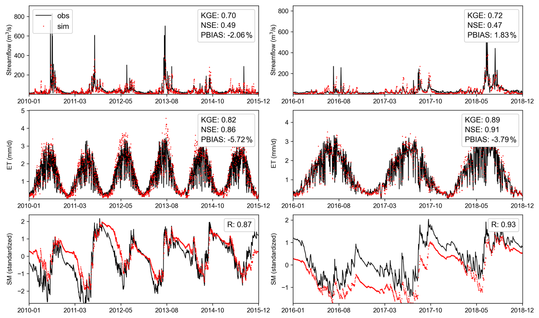
Figure 7 Daily simulated versus observed values under three-objective calibration, including streamflow, actual evaporation (ET), and standardized soil moisture. The left panels represent the calibration period, and the right panels represent the validation period.

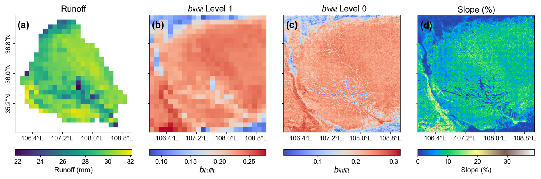
Figure 8 Spatial distribution of (a) total surface runoff, (b) b_infilt parameter at level-1 scale, (c) b_infilt parameter at level-0 scale, and (d) terrain slope.

5.3.2 Physical plausibility of spatial parameter patterns

A central concern in hydrological modelling is the reliability of spatial parameters, which are estimated from MPR in this study. Interpreting key VIC parameters in physically meaningful term is essential for establishing model credibility and ensuring “right results for right reason”. Here, we designed a synthetic single-peak rainfall event lasting two days with a total precipitation of 100 mm (Table 4), applied uniformly as the forcing input to the previously calibrated VIC model. The initial soil moisture was set to 70 % of the basin-average field capacity (θ_fc) for the upper two soil layers and 80 % of θ_fc for the bottom layer, to ensure consistent initial conditions across all grid cells. In this experiment, spatial variability arises solely from the model parameters fields. We therefore assess their physical plausibility by examining whether the resulting parameter-driven runoff patterns are consistent with general hydrological expectations.

Table 4 Meteorological conditions of the synthetic single-peak rainfall event.

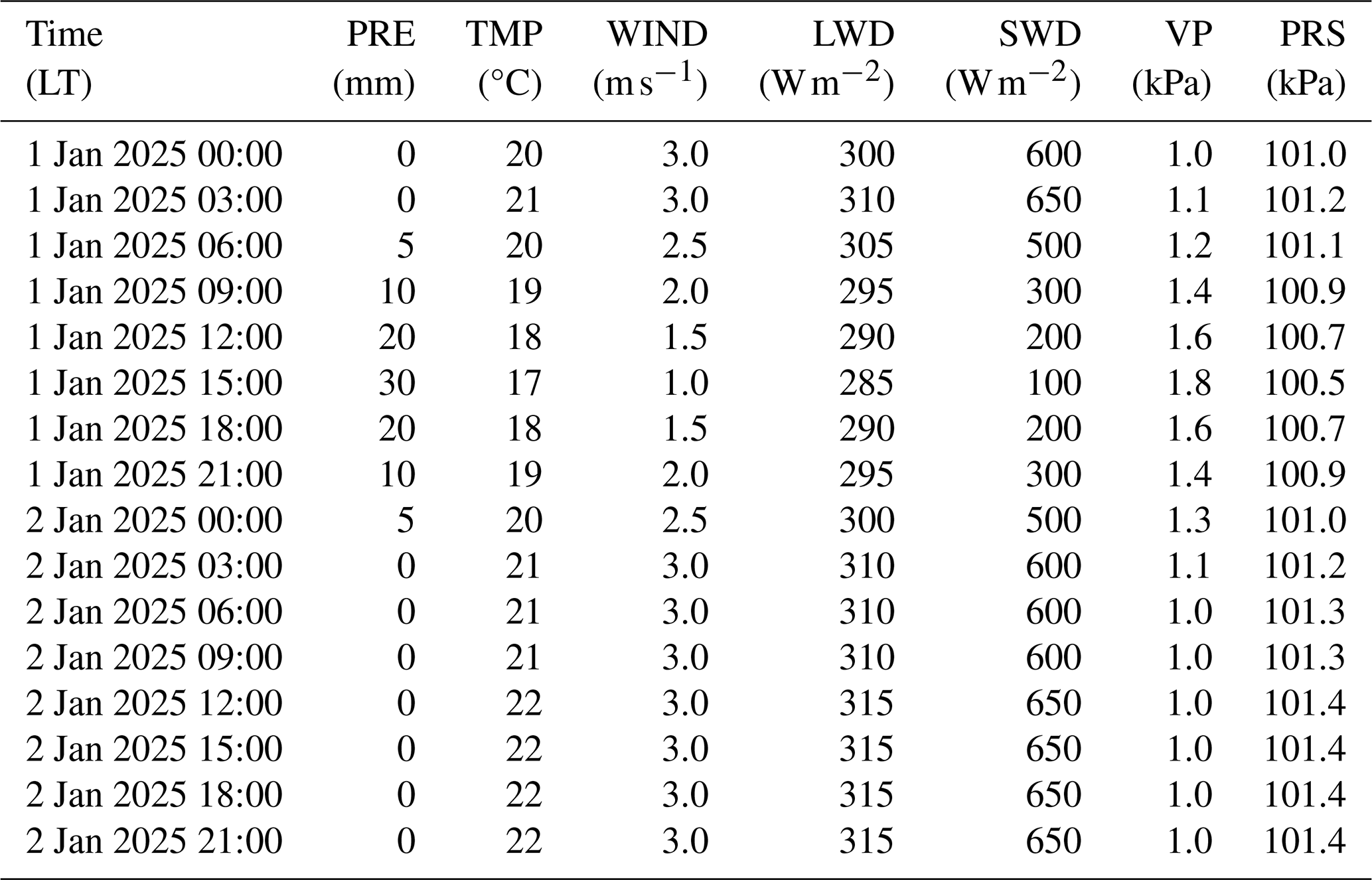
Note: PRE, precipitation; TMP, air temperature; WIND, wind speed; LWD, downward longwave radiation; SWD, downward shortwave radiation; VP, vapor pressure; PRS, surface pressure.

We first examined the relationship between total surface runoff and the abstract variable infiltration curve parameter (b_infilt), which has been identified in previous studies as a highly sensitive parameter in the VIC model (Gou et al., 2020). As shown in Fig. 8, the the spatial distribution of slope is strongly reflected in the runoff map, with areas characterized by lower terrain slopes exhibiting reduced runoff generation, such as the central part of the basin, the northwestern and southeastern corner. This pattern is physically plausible, as the general understanding of hillslope hydrological processes suggests that relatively flat areas tend to produce less runoff than steeper mountainous regions. From a computational perspective, this correspondence arises from the application of the MPR technique, in which slope is explicitly incorporated as an input for estimating the b_infilt at the level-0 scale (Fig. 8c). During the subsequent upscaling from the level-0 to the level-1, b_infilt governs the partitioning of rainfall between infiltration and surface runoff, with higher values reducing infiltration and enhancing surface runoff (Carvalho et al., 2022). Compared with spatially uniform parameters, the MPR-based estimates appear to be more physically plausible.

Next, we focus on the baseflow process. As presented in Fig. 9a, the influence of topography on runoff is also reflected in the total baseflow, with low values observed in the central basin. Moreover, a north–low to south–high gradient is apparent around 36.375° N, which is in line with the runoff yield distribution previously simulated using the Water and Energy Transfer Processes (WEP) model (Zhang et al., 2023) and aligns with the regional north–south transition from semi-arid to semi-humid climatic conditions (Jia et al., 2015). Computationally, this behaviour is governed by W_S – the proportion at which nonlinear baseflow begins (Yeste et al., 2024) – derived from D₃ (Nijssen et al., 2001). In the drier northern regions with weaker soil water retention, soil texture leads to lower field capacity (θ_s) values (Fig. 9c–f), which in turn result in larger estimated W_S values, thereby reducing baseflow generation (Fig. 9a and b). This spatial variability of W_S agrees with the expected role of soil water availability in controlling nonlinear baseflow activation, highlighting the physical interpretability of the calibrated parameter.

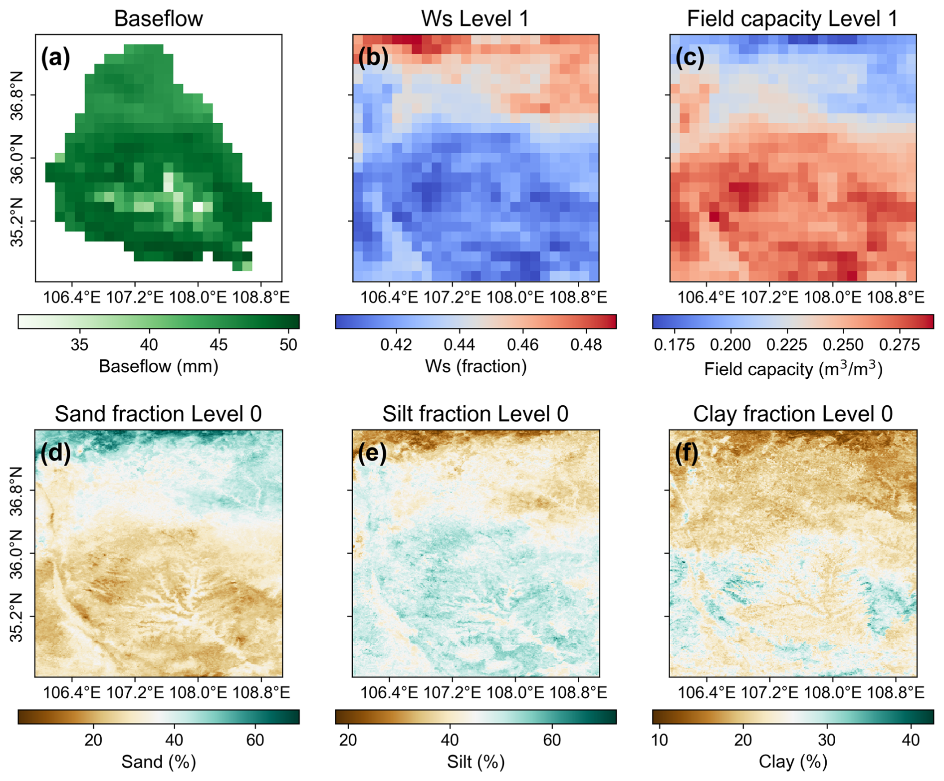
Figure 9 Spatial distribution of (a) total baseflow, (b) W_S parameter, (c) field capacity (θ_s), and (d–f) soil texture components: sand, silt, and clay fractions, respectively.

Finally, the plausibility of the estimated parameters was assessed through comparison with reference datasets from prior study. Specifically, two physically meaningful variables, field capacity (θ_s) and wilting point (θ_wp) were evaluated against the Soil Hydraulic Parameters for China released by Dai et al. (2013), which has been widely adopted in hydrological and land surface modeling applications (Miao et al., 2020; Gou et al., 2021). The corresponding spatial distributions are shown in Fig. 10. Clearly, both θ_s and θ_wp preserve the spatial patterns of the reference values after calibration, with a pronounced south-to-north decreasing gradient that reflects the higher soil water retention capacity in the southern JRB. In terms of magnitude, the calibrated θ_s values fall within nearly the same range as the reference values, while the θ_wp values are slightly higher; considering differences in soil layer conceptualization and potential scale effects, these discrepancies are deemed acceptable.

Figure 10 Spatial distribution of field capacity (θ_s) and wilting point (θ_wp). Panels (a) and (c) show parameters estimated through model calibration, while panels (b) and (d) are derived from Dai et al. (2013).

In summary, the above results support the physical plausibility of the estimated parameters, as reflected in their consistency with runoff processes and reference dataset. Furthermore, the coherence between the underlying input data (soil properties and topography) and the highly abstract parameters underscores the rationality of MPR-based parameter estimation, which is facilitated by the use of transfer functions (Mizukami et al., 2017).

6 Discussion

6.1 Opportunities and challenges of spatial parameter estimation in distributed hydrological models

The rapid growth of hydrological big data has enabled substantial advances in hydrological modelling, particularly in the development of increasingly sophisticated distributed models (Argentin et al., 2025). By explicitly representing the spatial variability of hydrological processes, distributed models can resolve the spatial patterns of hydrological states and fluxes that are unavailable from their lumped counterparts, offering valuable insights for water resources management and flood and drought risk assessment. For example, in this study we found that baseflow was generally more abundant in the southern part of the JRB, indicating potentially greater hydrological capacity to support afforestation in these areas (Fig. 9c). In contrast, the relatively lower baseflow in the northern part suggests that afforestation need to be implemented more cautiously to avoid increasing pressure on local water availability. In this context, integrating the increasingly available data sources for spatial parameter estimation presents new opportunities for fully realizing the potential of distributed hydrological modelling.

Several fundamental challenges hinder the effective estimation of spatially distributed parameters. First, the historical reliance on the concept of “effective parameters” in hydrological modelling has resulted in many models retaining a large number of free parameters that require calibration and are implicitly assumed to be spatially homogeneous, limiting their ability to explicitly represent spatial heterogeneity. Second, introducing spatially varying parameters into traditional calibration frameworks substantially increases the dimensionality of the optimization problem, while the available observations are often insufficient to constrain such high-dimensional parameter spaces, leading to equifinality and ill-posedness. Finally, direct parameter estimation approaches generally require extensive prior information describing the relationships between parameters and environmental characteristics, while establishing such relationships requires extensive experimental investigations and coordinated efforts across multiple disciplines. Against this background, many distributed hydrological models still use spatially uniform parameters to maintain the number of free parameters at a level that can be reliably constrained through calibration, imposing substantial limitations on their capability to represent spatial heterogeneity. Our previous studies have shown that such simplifications create spatial trade-offs that undermine the physical realism of simulations and limit predictive performance (Zheng et al., 2026).

To address these challenges, several strategies have been proposed for estimating spatially distributed parameters. A straightforward approach is to aggregate the modelling domain into spatial units, such as sub-basins, and independently calibrate parameters for each unit while assuming spatial homogeneity within it. This provides an intermediate representation between fully lumped and grid-based parameterizations, with implementations including spatial clustering (Huynh et al., 2024), representative grid sampling (Sun et al., 2021), and hydrological response units (HRUs). Nevertheless, the number of calibration parameters still increases with the number of spatial units, leaving the parameter-dimensionality problem largely unresolved. Another class of approaches can be broadly termed scaling methods, which infer parameter values at one spatial scale and relate them to hydrological processes or parameters at another through scale-invariant or explicitly scale-dependent relationships (Viney and Sivapalan, 2004). For example, Barrios and Frances (2012) demonstrated the feasibility of estimating mesoscale effective parameters by aggregating microscale simulation outputs and solving the inverse problem. Regionalization approaches further extend this concept and exploit similarity principles (Bao et al., 2012), establishing relationships between catchment characteristics and parameters in data-rich regions (donors) and transferring them to data-scarce or ungauged regions (receptors). More importantly, if such relationships are applied consistently across all modelling grids, they can provide an effective pathway for spatial parameter estimation.

Within the regionalization framework, MPR offers several advantages over conventional approaches. As mentioned in Sect. 3.1, MPR establishes environment–parameter relationships using transfer functions informed by existing literature. Compared with standard regionalization (SR) methods based on empirical regression or similarity measures derived from spatial distance or physical attributes, this approach allows prior knowledge from multiple disciplines to be explicitly incorporated into parameter estimation, thereby improving the plausibility and reliability of spatial parameter estimates (Mizukami et al., 2017). Meanwhile, the limited number of adjustable parameters in transfer functions maintains the parameter dimensionality within a practically calibratable range. In terms of cross-scale issues, MPR first derives high-resolution parameter fields and then aggregates them to the target modelling scale, shifting the scale transformation from environmental inputs to parameters across different resolutions. This provides the benefit of minimizing uncertainties associated with environmental data aggregation and improving the representation of subgrid parameter heterogeneity. As evidenced by Samaniego et al. (2010), MPR exhibited superior performance to SR in maintaining water balance and preserving the spatial patterns of simulated variables, whereas the latter introduced larger deviations during the upscaling process. Given these advantages, MPR was selected as the default spatial parameter estimation approach in EVB. Beyond this implementation, we envision that future developments of EVB should further investigate scale-aware parameterization by incorporating scaling factor into transfer functions, allowing nonlinear upscaling relationships to be integrated into the spatial parameter estimation procedure. In our view, advancing spatial parameter estimation approaches in this direction represents one of the key priorities for hydrological model development over the coming decade.

6.2 The positioning and scope of EVB

Positioning EVB within the existing VIC deployment ecosystem helps clarify its role and scope. Given the limited number of deployment tools available for VIC, we selected three representative examples, VIC-ASSIST, TONIC, and CyberWater, each briefly introduced in the Introduction, for comparison with EVB. We compiled a feature matrix covering supported VIC versions, implementation languages and distribution forms, approaches to parameter specification and regionalization, workflow reproducibility, and extensibility (Table 5). All three tools in the comparison are freely available, and several are distributed under open-source licenses (e.g. MIT license). This accessibility is consistent with the recommendation of Knoben et al. (2022) to use permissively licensed workflow components that support reuse and extension. However, free access to a deployment tool does not eliminate software dependencies. As noted earlier, VIC-ASSIST depends on MATLAB and ArcGIS, whose commercial licensing requirements may limit its use where these software packages are unavailable.

Table 5 Feature comparison of EVB with existing VIC deployment tools.

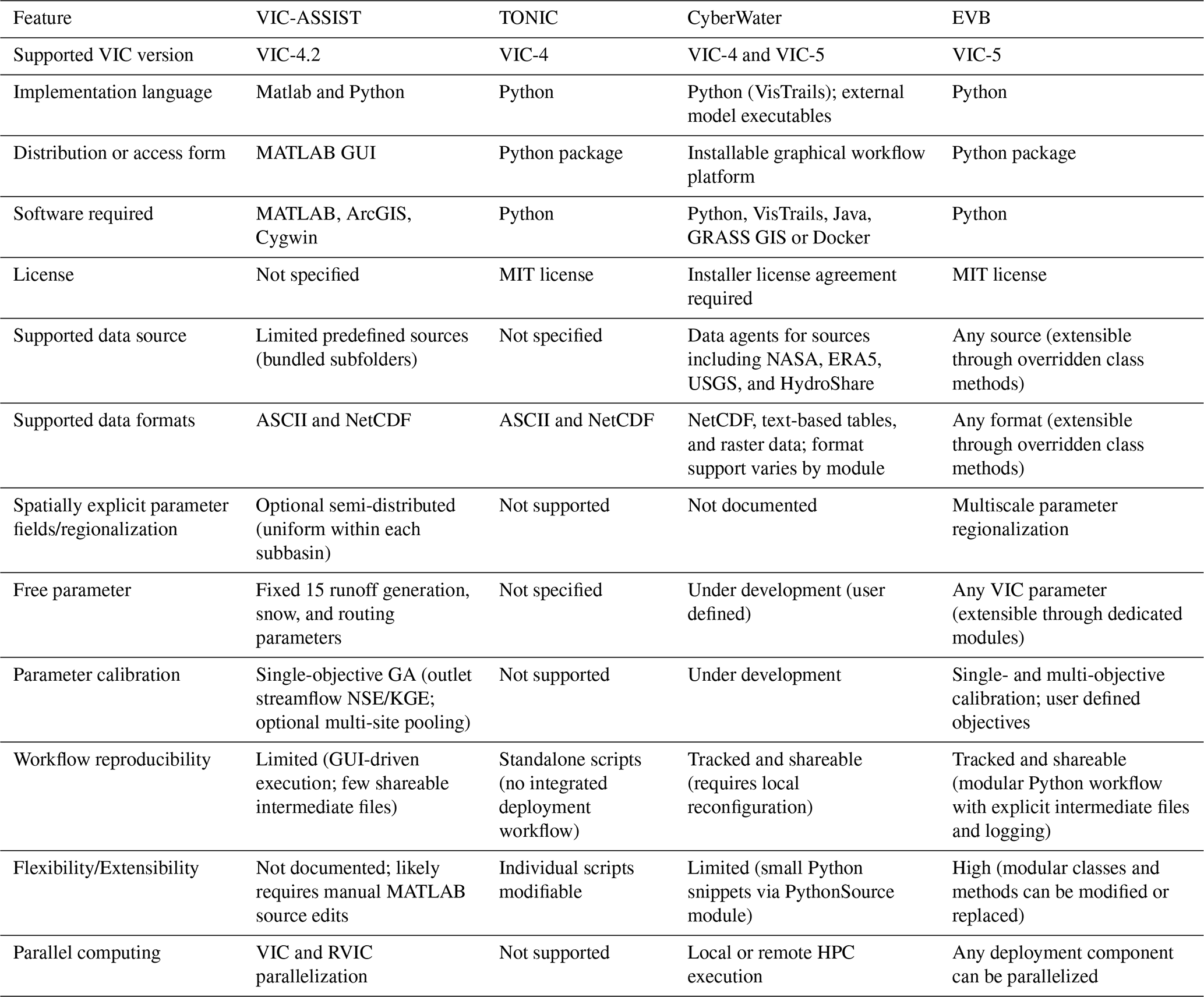
Note: GUI, graphical user interface; GA, genetic algorithm; MIT, Massachusetts Institute of Technology License; HPC, high performance computing; GRASS GIS, Geographic Resources Analysis Support System Geographic Information System; Docker, a containerization platform.

Functionally, TONIC has the narrowest scope among the four tools. It provides a small set of utility scripts, mainly for NetCDF and ASCII conversion and data visualization. It therefore does not constitute an integrated deployment workflow. VIC-ASSIST focuses on the rapid deployment of VIC 4 and simplifies operation by fixing several model choices, such as data sources and parameter calibration settings. This design is more suitable for new users and educational applications (Wi et al., 2017). By comparison, CyberWater combines a graphical interface with data and model agents, offering a practical balance between ease of use and functional breadth. It is accessible to users with limited programming experience and provides more configuration options than VIC-ASSIST. However, its encapsulated software architecture makes the workflow less straightforward to extend. For example, incorporating a new optimization algorithm may leave users or developers to adapt or reimplement the algorithm in the format expected by the workflow, rather than directly reusing an existing implementation from the broader Python ecosystem. EVB places greater demands on users' Python programming experience. In return, it provides direct control over every stage of the deployment workflow, from data preparation and parameter specification to calibration and parallel execution, supporting a broader range of advanced modelling applications (Table 5). Given the rapid development of large language model based programming tools, such as Codex, we believe that this programming requirement is unlikely to constitute a major barrier to the use of EVB.

Knoben et al. (2022) developed a workflow blueprint for the coupled SUMMA and mizuRoute modelling system as part of the CWARHM initiative. The blueprint has provided a reference for workflow based modelling in the Earth system science community by setting out guidelines for improving reproducibility through four key properties: separability, clarity, modularity, and traceability. Within this broader context, several aspects of the EVB design are consistent with the guidelines. First, EVB follows the separation of concerns (SoC) principle through a modular, loosely coupled, object-oriented design, allowing individual components to be modified or replaced independently. For example, the two basin setups examined here use CONUS SOIL and SoilGrids1km, respectively. The two datasets represent soil profiles using 11 layers spanning 0–250 cm and 6 layers spanning 0–200 cm. During parameter generation, EVB calls the same buildParameter function with two subclasses of SoilLayerResampler, one for each dataset. Each subclass requires only minimal overrides of selected methods, allowing the same function to accommodate both layer schemes without separate construction functions. This degree of component flexibility is not readily available in the other three tools. Consistent module interfaces also support workflow reproducibility. When Model A and Model B use the same data source, the dpc class can reuse the relevant modules within extractData_func without creating conflicts with other methods. Second, a structured directory design facilitates the exchange of workflows within the modelling community. Applications deployed with EVB follow a common directory structure managed by the Evb_dir class (Fig. 1c), allowing users to inspect and rapidly reuse existing studies. This design provides transparency while retaining flexibility for user defined extensions, a combination that is often difficult to achieve in graphical workflow systems. Third, EVB provides flexibility at two levels: runtime configuration of model options and extension beyond the original application scope. Its ability to combine alternative modelling decisions was demonstrated in our previous study (Zheng et al., 2026), in which flexible deployment enabled eight cases with different combinations of spatial discretization and calibration configuration. By contrast, deployment frameworks that do not expose their underlying code may offer only limited scope for extension, with further development often depending primarily on the original developers. Taken together, these features position EVB to improve transparency within the VIC modelling community, facilitate the exchange of computational practices, and reduce duplicated effort across the broader scientific community. By making deployment procedures easier to inspect, reproduce, and extend, EVB may also accelerate the iterative development and refinement of VIC.

Last but not least, the current scope of EVB warrants further consideration. Its reliance on GeoDataFrame structures may become inefficient for very large domains at continental or global scales, where chunked and parallel processing with Dask (https://docs.dask.org, last access: 2 November 2026) or comparable tools may be needed. In addition, the transferability of MPR derived parameter estimates has so far been evaluated over a limited range of spatial scales, and broader testing is therefore needed. Future development will focus on four directions: (1) introducing a standardized data layer between preprocessing stages, thereby allowing framework specific intermediate files to be replaced with interoperable formats, notably GeoTIFF and NetCDF; (2) developing interfaces for conversion between VIC versions to improve backward compatibility; (3) implementing vector-based modelling units to provide more flexible spatial representations; and (4) maintaining consistency with ongoing VIC development, particularly its Python driver, which is currently experimental and remains under development. Future integration with this driver could broaden the scope of EVB, improve compatibility with VIC, and contribute to the continued development of the VIC modelling ecosystem.

7 Conclusion

This study was motivated by the need for a standardized and reproducible approach to VIC model deployment. Although the restructuring of VIC-5 has improved the model's flexibility and maintainability, it has also increased the technical complexity of its implementation. To address this challenge, we developed Easy VIC Build (EVB), an open source Python framework that supports flexible and efficient automated deployment of VIC-5. EVB adopts a modular object-oriented architecture and integrates advanced deployment techniques, including the Multiscale Parameter Regionalization (MPR) and the General Unit Hydrograph (GUH). Through the implementation of several core classes – such as Grids and Basins for storing and processing geographic information, dpc for managing forcing and general input data, and Evb_dir for organizing file paths – together with a layered abstraction strategy based on information-level division, EVB enables efficient data management and seamless information transfer throughout the model deployment workflow.

The efficiency of the EVB framework was evaluated through several real-world modelling applications involving two distinct basin setups. In the first setup, parameters estimated with EVB transferred robustly across spatial resolutions. Transfers from the 12 km resolution to the 8 and 6 km resolutions reduced KGE values by less than 0.1 while largely preserving the spatial patterns of simulated runoff. In the second setup, VIC models deployed with EVB supported multi-objective calibration and simulation, yielding KGE values above 0.7 for streamflow and 0.8 for actual evapotranspiration. The correlation coefficients between simulated and observed soil moisture also exceeded 0.85. The results further support the effectiveness and physical plausibility of the spatial parameter fields estimated with MPR. These fields were consistent with both the spatial distribution of simulated runoff and an independent reference dataset of soil parameters. Regarding deployment efficiency, data preprocessing and meteorological forcing generation were the most time-consuming steps. However, because each step needs to be performed only once, the associated computational costs remained acceptable. Overall, these results indicate that EVB can facilitate broader applications of VIC by improving compatibility with VIC-5 and providing a flexible, reproducible and efficient deployment framework that extends the capabilities of existing tools.

Appendix A: Free parameters calibrated in the Easy VIC Build framework

Table A1 Full set of 44 free parameters for calibration (Guo, 2022; Lohmann et al., 1996; Mizukami et al., 2017).

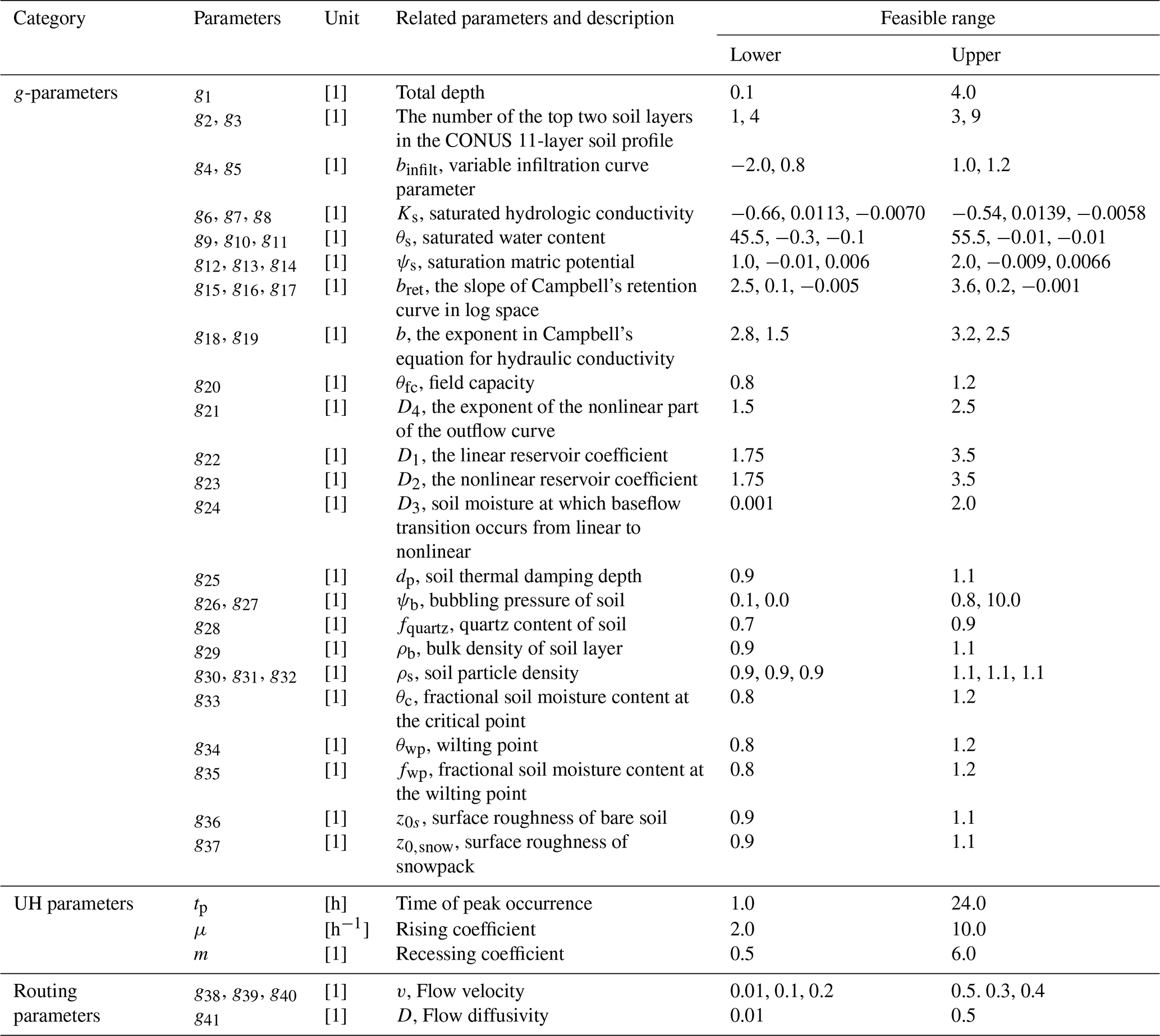
Table A2 Summary of the transfer functions and their formulation sources for VIC-specific parameterization in EVB.

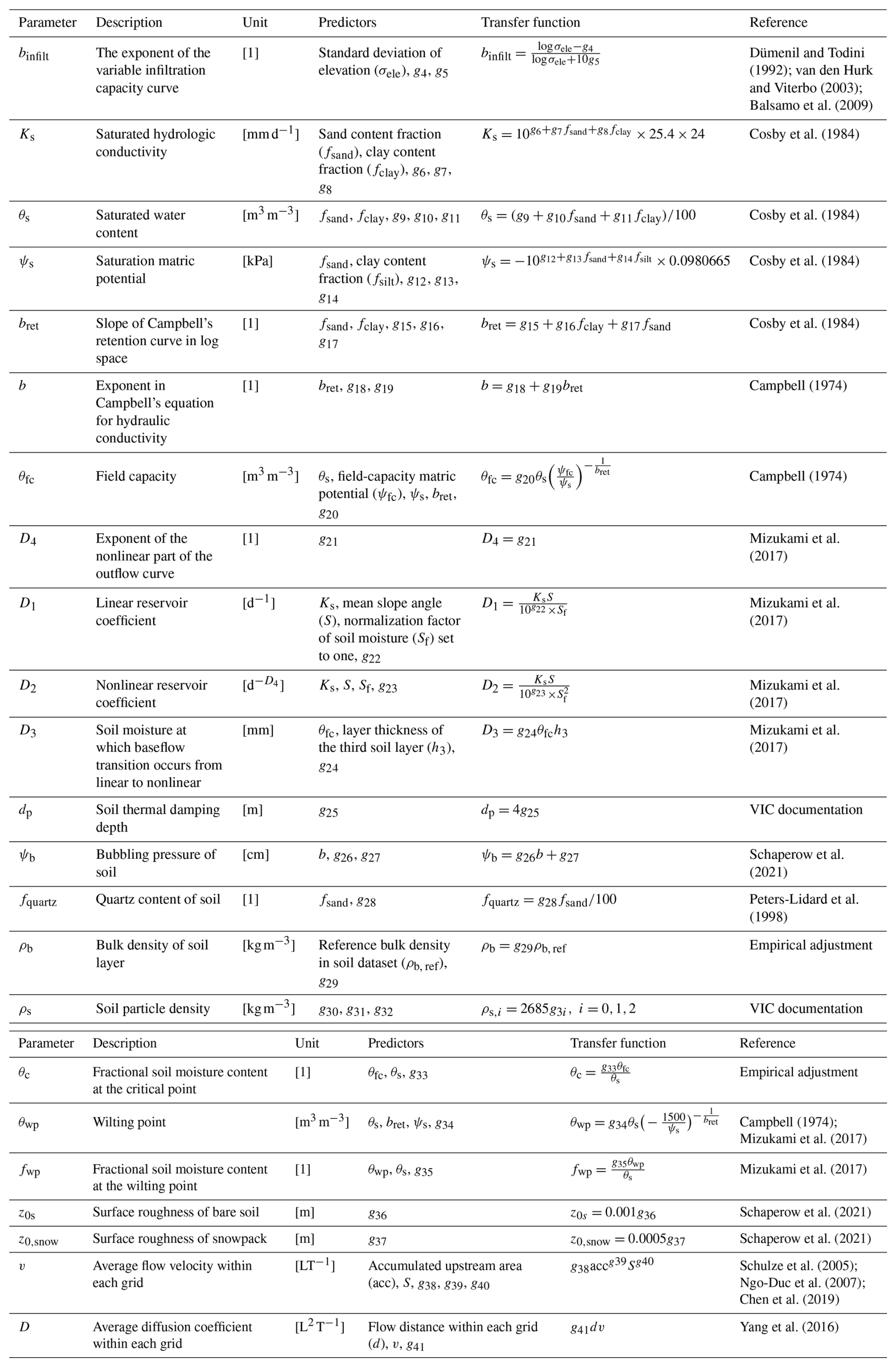
Note: Units are S (%), h₃ (m), acc (km²), and d (m). ψ_fc is set to −33, −20, and −10 kPa when f_sand≤50 %, $\text{50\hspace{0.17em}\%}<f_{\text{sand}}\le \mathrm{70}$ %, and f_sand>70 %, respectively. The source of VIC documentation is: https://vic.readthedocs.io/en/master/ (last access: 2 November 2026).

Table A3 Simplified set of 15 free parameters for calibration.

Appendix B: Model calibration process under single and multiple objective settings

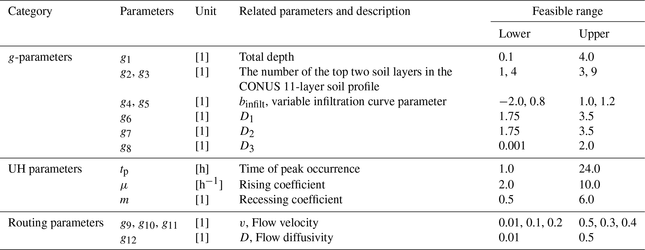
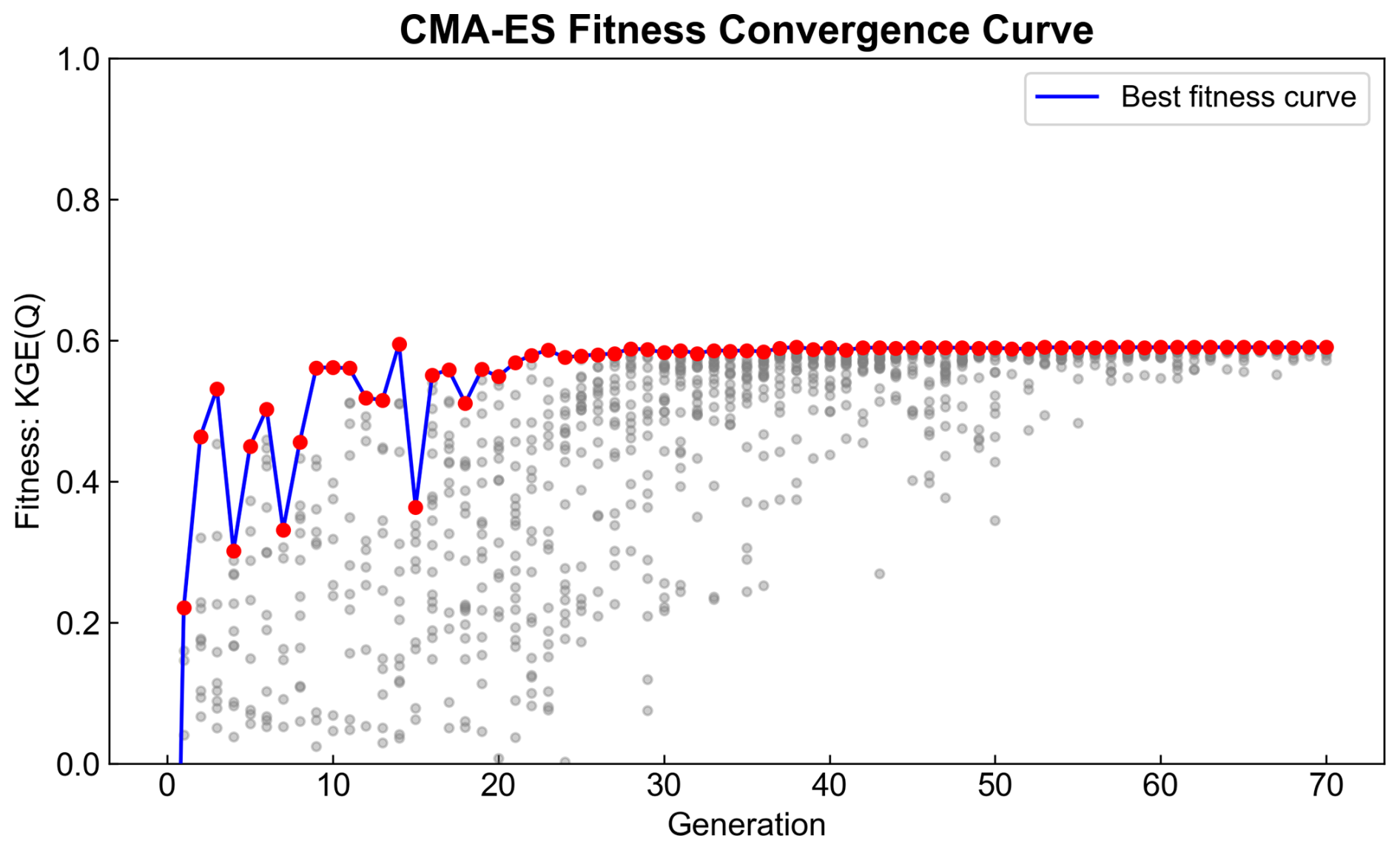
Figure B1 Convergence curve obtained from the single-objective calibration for Basin Setup A, with the Kling–Gupta efficiency (KGE) of streamflow (Q) as the objective. The maximum fitness shows convergence after around 20 generations, whereas population-level convergence is observed after approximately 50 generations.

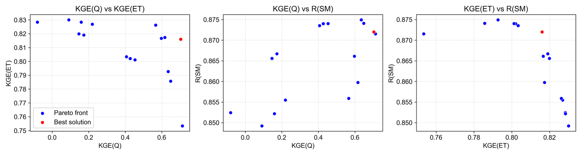
Figure B2 Pareto front curves obtained from the multi-objective calibration for Basin Setup B, with three objectives including the Kling–Gupta efficiency (KGE) of streamflow (Q), the KGE of actual evapotranspiration (ET), and the correlation coefficient (R) of standardized soil moisture (SM). A certain degree of trade-off is observed between KGE (ET) and KGE (Q) as well as KGE (ET) and KGE (SM), while KGE (Q) and R (SM) tend to show a more synergistic behaviour.

Appendix C: VIC streamflow simulations at 8 and 6 km using parameter transferred from 12 km calibration

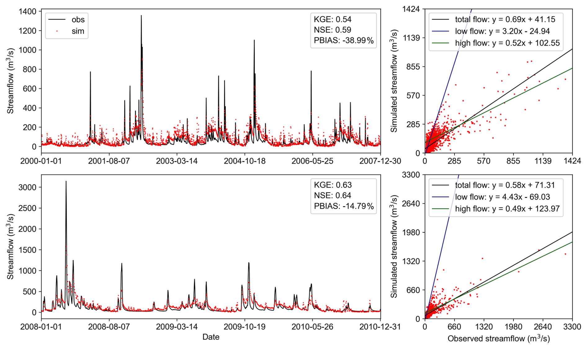
Figure C1 Comparison of daily simulated streamflow from the 8 km-resolution VIC model against observations during the calibration period (top two panels) and validation period (bottom two panels). Low-flow and high-flow thresholds are defined as the 30th and 70th percentiles of the total flow range, respectively.

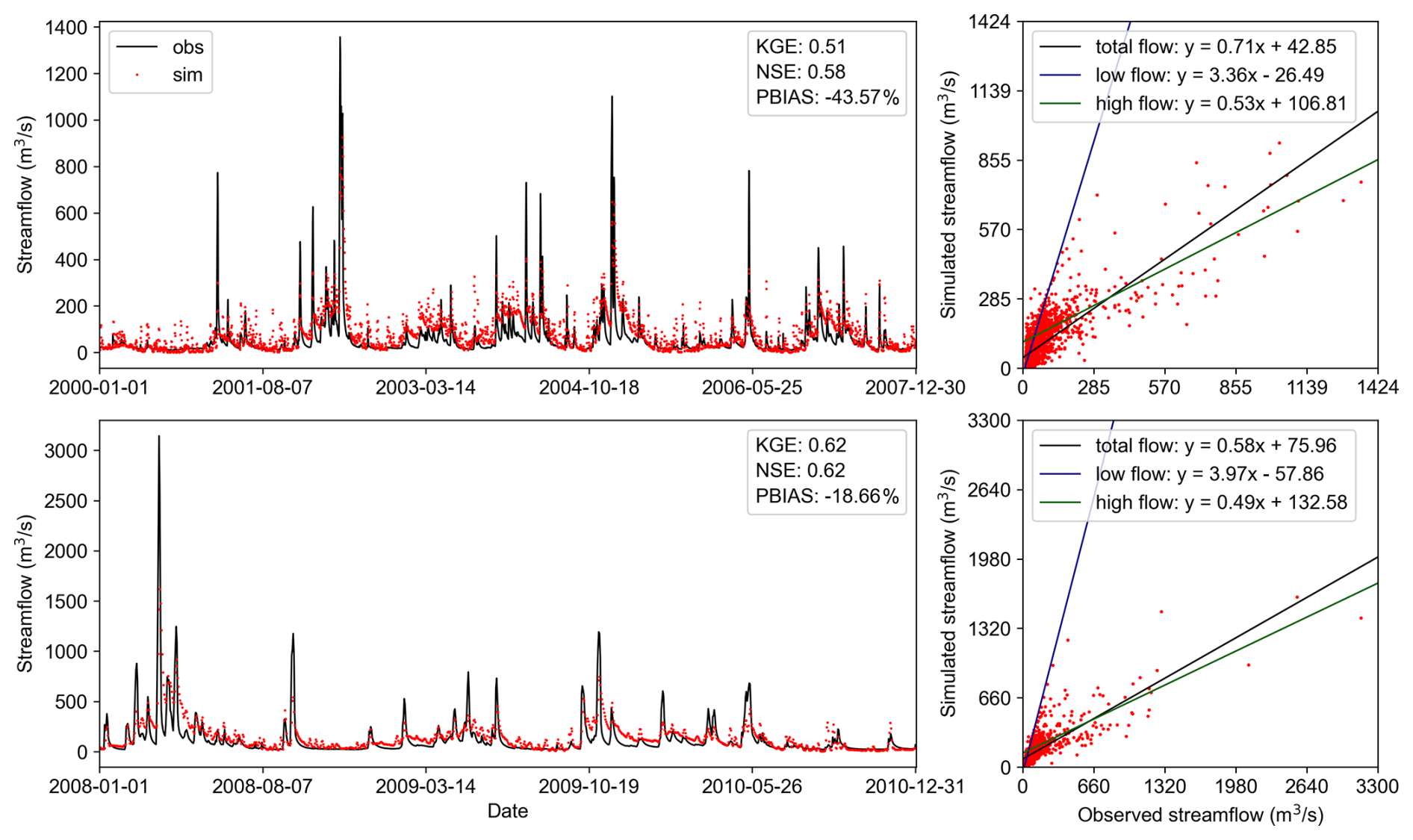
Figure C2 Comparison of daily simulated streamflow from the 6 km-resolution VIC model against observations during the calibration period (top two panels) and validation period (bottom two panels). Low-flow and high-flow thresholds are defined as the 30th and 70th percentiles of the total flow range, respectively.