Hybrid implicit–explicit XFEM simulation of injection-induced seismicity: resolving multi-scale rupture nucleation and dynamics

This study presents a novel hybrid implicit–explicit time-integration strategy for simulating injection-induced fault reactivation within a fully coupled poroelastodynamic extended finite element (XFEM) framework. Modeling these systems is inherently challenging due to the extreme separation of temporal scales – ranging from hours to days for fluid diffusion to milliseconds for dynamic rupture. Although the fully implicit formulation can provide enhanced numerical stability, stability alone does not guarantee sufficient temporal accuracy during nonlinear fault rupture. The results demonstrate close agreement between simulations with minimum time-step sizes of 10⁻⁵ and 10⁻⁶ s for the investigated slip and event-scale observables on the adopted spatial mesh, indicating temporal convergence for these quantities at 10⁻⁵ s. This time-step size is substantially smaller than the mesh-based explicit stability estimate. To reduce computational cost, the proposed strategy employs an implicit solver for quasi-static loading and nucleation and switches to a central-difference-based mechanical solver with implicit pressure integration once a prescribed slip-velocity threshold is exceeded. At a switching threshold of 0.01 m s⁻¹, the hybrid simulation requires approximately 10.0 h, compared with 26.4 h for the fully implicit reference, corresponding to a computational-time reduction of 62.12 %. The hybrid strategy reproduces the overall rupture sequence, stress evolution, final accumulated fault slip, and seismic moment. However, differences remain in the timing and magnitude of peak slip velocities, rupture-propagation speeds, and transient particle motion. These findings demonstrate the computational potential of the hybrid formulation for the investigated two-dimensional configuration, while highlighting the need for further assessment of transient dynamic accuracy and computational performance across different spatial discretizations and geological conditions.

1 Introduction

The increasing reliance on subsurface technologies such as enhanced geothermal systems (EGS) and carbon capture and storage (CCS) has become a cornerstone of modern energy transition and climate-mitigation strategies. Despite their societal benefits, these operations inevitably involve large-scale fluid injection into the crust, which has been repeatedly associated with injection-induced seismicity (Cao et al., 2022; Grigoratos et al., 2022; Cheng et al., 2023; Templeton et al., 2023; Zhou et al., 2024; Sun et al., 2026). Induced seismicity poses significant operational, regulatory, and societal challenges (Grigoli et al., 2017; Trutnevyte and Ejderyan, 2018; Bommer, 2022), particularly when events exceed acceptable risk thresholds. Consequently, accurately simulating the mechanisms controlling the timing, magnitude, and spatial evolution of induced earthquakes remains a key scientific and engineering objective.

Injection-induced seismicity arises from the coupled interactions of multiple physical processes, including pore-pressure diffusion, thermoporoelastic stress redistribution, and frictional weakening along pre-existing faults (Boyet et al., 2023; Kivi et al., 2023). Capturing this complexity in numerical models requires to fully resolve the details of the coupling among these physical processes while also incorporating advanced fracture constitutive laws that govern fault strength and deformation (Cueto-Felgueroso et al., 2018; Riga and Turuntaev, 2021; Heimisson et al., 2022; Ito et al., 2023; Gerardi et al., 2024; Ito et al., 2024; Im and Avouac, 2025; Hosseini et al., 2025). While significant progress has been made in describing frictional fault behavior, its practical application to realistic injection scenarios remains computationally demanding.

A key challenge stems from the extreme separation of temporal scales inherent to injection-driven fault reactivation. Reservoir pressurization and fluid diffusion typically evolve over hours to days, whereas fault nucleation and dynamic rupture unfold over less than milliseconds to seconds (Han and Younis, 2023). To accurately resolve both regimes within a single simulation places stringent demands on time integration schemes. Fully implicit methods are commonly adopted because of their unconditional stability and efficiency during long periods of quasi-static loading (Jin and Zoback, 2018; Romanet et al., 2025). However, once rapid fault acceleration begins, these schemes require very small time steps and repeated global Newton iterations to maintain accuracy, leading to prohibitive computational costs. In contrast, explicit schemes are well-suited for dynamic rupture due to their low per-step cost and straightforward treatment of inertia, but their strict Courant–Friedrichs–Lewy (CFL) stability constraint (Alkhimenkov et al., 2021) renders them impractical for simulating long-term fluid injection and slow nucleation phases.

This fundamental trade-off between stability, accuracy, and efficiency highlights a methodological gap: no single time-integration strategy is optimal across the full spectrum of processes governing injection-induced seismicity. Addressing this limitation is essential to advance numerical simulations that are both accurate during rupture and tractable over operational time scales. While transitions from slow quasi-static or quasi-dynamic deformation to fully dynamic rupture have been previously addressed in earthquake-cycle and rupture simulations (Jin and Zoback, 2018; Pampillon et al., 2018; Katsman and Ben-Avraham, 2025), here we develop and implement a hybrid time-integration framework within a fully coupled poroelastodynamic XFEM formulation to reduce the computational cost of injection-induced fault reactivation simulations. The proposed approach advances the system implicitly during quasi-static loading and nucleation, and automatically transitions to a fully dynamic explicit formulation once a slip-velocity threshold indicative of unstable rupture is exceeded. This switching parameter enables a consistent and adaptive treatment of multi-scale processes within a single computational framework. The implicit formulation developed here serves as a robust reference solution and represents an improvement to our previous effort in modeling fault rupture process (Sabah et al., 2026). Building on this foundation, we demonstrate that the hybrid implicit–explicit solver-switching strategy preserves the accuracy of fault slip, stress evolution, and seismic source parameters, while substantially reducing computational costs under evolving subsurface conditions.

The remainder of the paper is organized as follows. Section 2 details the methodological framework, including the coupled hydromechanical equations, rate-and-state friction model, and XFEM-based spatial discretization. This section also introduces the reference fully implicit scheme, a modified version of our previous work, and the hybrid solution strategy with its switching criteria. Section 3 discusses the model validation, including benchmark problems used to verify the coupled formulation and numerical implementation, and outlines the numerical model setup, including geometry, material properties, and injection protocols. Section 4 presents numerical experiments that assess the influence of time-stepping on the implicit solver and compare the hybrid formulation against the reference in terms of accuracy and performance. Section 5 summarizes the main conclusions, while Sect. 6 discusses the limitations of the present study and possible directions for future work.

2 Mathematical formulations

2.1 Governing equations

The partial differential equations governing the isothermal deformation of faults in a porous medium comprise the balance of linear momentum for the solid–fluid system and the mass-conservation equations governing fluid flow through the faults and surrounding porous matrix. The dynamic balance of linear momentum is written as (Jaeger et al., 2009):

$$\begin{array}{}\text{(1)}& \mathrm{\nabla }\cdot \mathit{\sigma }-\mathit{\rho }\ddot{\mathit{u}}+\mathit{\rho }\mathit{b}=\mathrm{0}\end{array}$$

where σ is total stress tensor, $\ddot{\mathit{u}}$ is the solid acceleration, b is the body force vector, and ρ is density of saturated rock. Fluid flow in the porous matrix is described by Darcy's law, assuming a constant intrinsic permeability of the pore space. By coupling Darcy's law with the mass conservation principle, the governing equation for fluid flow in a poroelastic medium is obtained as follows (Wang, 2000):

$$\begin{array}{}\text{(2)}& \mathrm{\nabla }\cdot \left[\mathit{k}\left(-\mathrm{\nabla }p-{\mathit{\rho }}_{\mathrm{f}}\ddot{\mathit{u}}+{\mathit{\rho }}_{\mathrm{f}}\mathit{b}\right)\right]+\mathit{\alpha }\mathrm{\nabla }\cdot \dot{\mathit{u}}+S_{\mathrm{s}}\dot{p}=\mathrm{0}\end{array}$$

where p denotes the pore pressure, α is the Biot coefficient, k is the hydraulic mobility tensor, ρ_f is fluid density, and $S_{\mathrm{s}}=\left(\mathit{\varphi }{C}_{\mathrm{f}}+\frac{\left(\mathit{\alpha }-\mathit{\varphi }\right)\left(\mathrm{1}-\mathit{\alpha }\right)}{K}\right)$ denotes the specific storage coefficient with ϕ and K as porosity and drained bulk modulus, respectively, and C_f as fluid compressibility. Fluid flow within a fault obeys the same governing physical principles as flow in the surrounding porous medium; however, it is formulated over domain Ω^′ (Fig. 1). In contrast to the porous matrix, fault permeability is not assumed constant but evolves dynamically in response to variations in its hydraulic aperture. This behavior is represented using the cubic law, which links laminar flow along the fault to the cube of its aperture. Accordingly, fluid flow along the fault interface is governed by (Zimmerman and Paluszny, 2024):

$$\begin{array}{}\text{(3)}& \mathrm{\nabla }\cdot \left[{\displaystyle \frac{w^{\mathrm{2}}}{\mathrm{12}{\mathit{\mu }}_{\mathrm{f}}}}\left(-\mathrm{\nabla }p-{\mathit{\rho }}_{\mathrm{f}}\ddot{\mathit{u}}+{\mathit{\rho }}_{\mathrm{f}}\mathit{b}\right)\right]+\mathrm{\nabla }\cdot \dot{\mathit{u}}+C_{\mathrm{f}}\dot{p}=\mathrm{0},\mathrm{on}{\mathrm{\Omega }}^{\prime }\end{array}$$

where w represents the hydraulic aperture of the fault and μ_f is fluid viscosity. It should be noted that Eqs. (1)–(3) do not represent the full dynamic Biot poroelastic formulation. Instead, they correspond to a coupled u−p formulation, in which dynamic effects are introduced through the solid momentum balance and the acceleration term appearing in the hydraulic driving force. The full two-field inertial structure of dynamic Biot theory, including added-mass effects, tortuosity, and relative fluid acceleration terms, is not considered (Biot, 1956; Zienkiewicz and Shiomi, 1984). This approximation is appropriate for the present study, where the main objective is to resolve pore-pressure diffusion coupled with poroelastodynamic deformation, fault slip, and mechanical wave propagation in the porous skeleton, rather than to model the full dynamic Biot wave modes associated with relative fluid–solid acceleration in the saturated porous medium.

2.2 Variational formulation of flow and deformation in a fractured porous medium

The variational (weak) formulation is derived by multiplying the governing equations with suitable test functions and integrating over the computational domain. By invoking the Gauss–Green theorem in the presence of discontinuities, enforcing traction continuity across the contact interface, and incorporating Biot's theory to account for poromechanical effects at the interface, the weak form of the mechanical equilibrium (Eq. 1) includes contributions from both the bulk domain and the interface as:

$$\begin{array}{}\text{(4)}& \begin{array}{rl}& {\int }_{\mathrm{\Omega }}\mathrm{\nabla }\mathit{\delta }\mathit{v}:\mathit{\sigma }{}^{\prime }\mathrm{d}\mathrm{\Omega }-{\int }_{\mathrm{\Omega }}\mathrm{\nabla }\mathit{\delta }\mathit{v}:\left(\mathit{\alpha }p\mathit{m}\right)\mathrm{d}\mathrm{\Omega }+{\int }_{\mathrm{\Omega }}\mathit{\delta }\mathit{v}\cdot \mathit{\rho }\ddot{\mathit{u}}\mathrm{d}\mathrm{\Omega }\\ & +{\int }_{{\mathrm{\Gamma }}_{\mathrm{d}}}\left[[\mathit{\delta }\mathit{v}\right]]\mathit{t}\mathrm{d}\mathrm{\Gamma }-{\int }_{{\mathrm{\Gamma }}_{\mathrm{d}}}\left[[\mathit{\delta }\mathit{v}\right]]\left(p{\mathit{n}}_{{\mathrm{\Gamma }}_{\mathrm{d}}}\right)\mathrm{d}\mathrm{\Gamma }\\ & -{\int }_{\mathrm{\Omega }}\mathit{\delta }\mathit{v}\cdot \mathit{\rho }\mathit{b}\mathrm{d}\mathrm{\Omega }-{\int }_{{\mathrm{\Gamma }}_t}\mathit{\delta }\mathit{v}\cdot \left(\mathit{\sigma }{\mathit{n}}_{{\mathrm{\Gamma }}_t}\right)\mathrm{d}\mathrm{\Gamma }=\mathrm{0}\end{array}\end{array}$$

where σ^′ is effective stress tensor, δv is the test function for displacement, t is the traction vector on fault interface, $\mathit{m}={\left[\begin{array}{ccc}\mathrm{1}& \mathrm{1}& \mathrm{0}\end{array}\right]}^T$ is the Voigt representation of the second-order identity tensor, and ${\mathit{n}}_{{\mathrm{\Gamma }}_{\mathrm{d}}}$ and ${\mathit{n}}_{{\mathrm{\Gamma }}_t}$ are the unit normal vector to the fault interface Γ_d and the mechanical Neumann boundary Γ_t, respectively. In an analogous manner, the weak formulation of the fluid flow equation in the porous matrix is derived by multiplying the governing equation (Eq. 2) by the pressure test function δψ and integrating over the domain:

$$\begin{array}{}\text{(5)}& \begin{array}{rl}& {\int }_{\mathrm{\Omega }}\mathrm{\nabla }\mathit{\delta }\mathit{\psi }\mathit{k}\mathrm{\nabla }p\mathrm{d}\mathrm{\Omega }+{\int }_{\mathrm{\Omega }}\mathrm{\nabla }\mathit{\delta }\mathit{\psi }\mathit{k}\cdot {\mathit{\rho }}_{\mathrm{f}}\ddot{\mathit{u}}\mathrm{d}\mathrm{\Omega }-{\int }_{{\mathrm{\Gamma }}_{\mathrm{d}}}\mathit{\delta }\mathit{\psi }{\stackrel{\mathrm{‾}}{q}}_{\mathrm{f}}\mathrm{d}\mathrm{\Gamma }\\ & +{\int }_{\mathrm{\Omega }}\mathit{\delta }\mathit{\psi }\mathit{\alpha }\mathrm{\nabla }\cdot \dot{\mathit{u}}\mathrm{d}\mathrm{\Omega }+{\int }_{\mathrm{\Omega }}\mathit{\delta }\mathit{\psi }{S}_{\mathrm{s}}\dot{p}\mathrm{d}\mathrm{\Omega }-{\int }_{\mathrm{\Omega }}\mathrm{\nabla }\mathit{\delta }\mathit{\psi }\mathit{k}\cdot {\mathit{\rho }}_{\mathrm{f}}\mathit{b}\mathrm{d}\mathrm{\Omega }\\ & +{\int }_{{\mathrm{\Gamma }}_{\mathrm{w}}}\mathit{\delta }\mathit{\psi }\left(\mathit{q}\cdot {\mathit{n}}_{{\mathrm{\Gamma }}_{\mathrm{w}}}\right)\mathrm{d}\mathrm{\Gamma }=\mathrm{0}\end{array}\end{array}$$

where $\mathit{q}=\mathit{k}\left(-\mathrm{\nabla }p-{\mathit{\rho }}_{\mathrm{f}}\ddot{\mathit{u}}+{\mathit{\rho }}_{\mathrm{f}}\mathit{b}\right)$ is Darcy flux vector field in porous media, Γ_w is hydraulic Neumann boundary, and ${\stackrel{\mathrm{‾}}{q}}_{\mathrm{f}}$ represents the fluid flux component normal to the fault interface, describing the exchange of fluid between the fault and the rock matrix. The weak form of the flow continuity equation within the fault is derived by multiplying Eq. (3) by the test function δψ(x,t) and integrating over fault domain Ω^′ (as illustrated in Fig. 1), resulting in (Khoei, 2015):

$$\begin{array}{}\text{(6)}& \begin{array}{rl}& {\int }_{\mathrm{\Omega }{}^{\prime }}\mathrm{\nabla }\mathit{\delta }\mathit{\psi }{\displaystyle \frac{w^{\mathrm{2}}}{\mathrm{12}{\mathit{\mu }}_{\mathrm{f}}}}\mathrm{\nabla }p\mathrm{d}\mathrm{\Omega }+{\int }_{\mathrm{\Omega }{}^{\prime }}\mathrm{\nabla }\mathit{\delta }\mathit{\psi }{\displaystyle \frac{w^{\mathrm{2}}}{\mathrm{12}{\mathit{\mu }}_{\mathrm{f}}}}{\mathit{\rho }}_{\mathrm{f}}\ddot{\mathit{u}}\mathrm{d}\mathrm{\Omega }\\ & -{\int }_{{\mathrm{\Gamma }}_{\mathrm{d}}}\mathit{\delta }\mathit{\psi }{\stackrel{\mathrm{‾}}{q}}_{\mathrm{f}}\mathrm{d}\mathrm{\Gamma }+{\int }_{\mathrm{\Omega }{}^{\prime }}\mathit{\delta }\mathit{\psi }\mathrm{\nabla }\cdot \dot{\mathit{u}}\mathrm{d}\mathrm{\Omega }+{\int }_{\mathrm{\Omega }{}^{\prime }}\mathit{\delta }\mathit{\psi }{C}_{\mathrm{f}}\dot{p}\mathrm{d}\mathrm{\Omega }\\ & -{\int }_{\mathrm{\Omega }{}^{\prime }}\mathrm{\nabla }\mathit{\delta }\mathit{\psi }{\displaystyle \frac{w^{\mathrm{2}}}{\mathrm{12}{\mathit{\mu }}_{\mathrm{f}}}}{\mathit{\rho }}_{\mathrm{f}}\mathit{b}\mathrm{d}\mathrm{\Omega }=\mathrm{0}\end{array}\end{array}$$

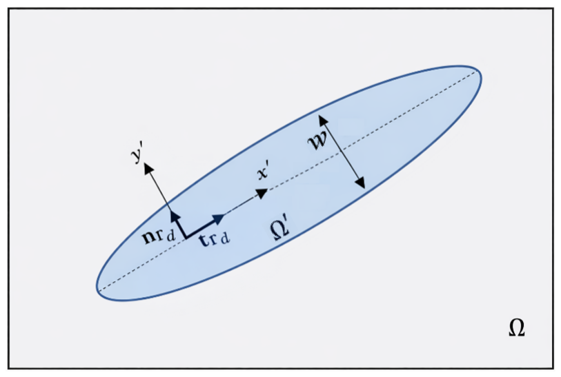
Figure 1 Schematic representation of the local coordinate system and fluid flow geometry within the fault. The blue elliptical-shaped region is used only to illustrate the hydraulic aperture w in cross-sectional view and should not be interpreted as the actual computational fault geometry. In the XFEM formulation, the fault domain Ω^′ is represented as a one-dimensional line embedded in the two-dimensional porous domain Ω. This is because the aperture is very small relative to the fault length, the pressure gradient across the aperture is neglected, and flow is modeled only along the fault direction x^′.

Equation (6) presents a unified variational formulation for hydro-mechanic coupled fluid flow within faults, enabling consistent fluid exchange between the fault and the surrounding porous matrix. The formulation is evaluated over domain Ω^′, using a fault-aligned local coordinate system (Fig. 1). Assuming negligible pressure gradients across the fault aperture, justified by the small fault width relative to its length, the cross-sectional integration is simplified by treating pressure as uniform across the aperture. Accordingly, a lower-dimensional representation of flow along the interface can be written as follows (Khoei, 2015):

$$\begin{array}{}\text{(7)}& \begin{array}{rl}& {\int }_{{\mathrm{\Gamma }}_{\mathrm{d}}}\mathrm{\nabla }\mathit{\delta }\mathit{\psi }\cdot {\mathit{t}}_{{\mathrm{\Gamma }}_{\mathrm{d}}}\left({\displaystyle \frac{w^{\mathrm{3}}}{\mathrm{12}{\mathit{\mu }}_{\mathrm{f}}}}\right)\mathrm{\nabla }p\cdot {\mathit{t}}_{{\mathrm{\Gamma }}_{\mathrm{d}}}\mathrm{d}\mathrm{\Gamma }+{\int }_{{\mathrm{\Gamma }}_{\mathrm{d}}}\mathrm{\nabla }\mathit{\delta }\mathit{\psi }\\ & \cdot {\mathit{t}}_{{\mathrm{\Gamma }}_{\mathrm{d}}}\left({\displaystyle \frac{w^{\mathrm{3}}}{\mathrm{12}{\mathit{\mu }}_{\mathrm{f}}}}{\mathit{\rho }}_{\mathrm{f}}\right)〈\ddot{\mathit{u}}〉\cdot {\mathit{t}}_{{\mathrm{\Gamma }}_{\mathrm{d}}}\mathrm{d}\mathrm{\Gamma }+{\int }_{{\mathrm{\Gamma }}_{\mathrm{d}}}\mathit{\delta }\mathit{\psi }w{\mathit{t}}_{{\mathrm{\Gamma }}_{\mathrm{d}}}\cdot 〈\mathrm{\nabla }\dot{\mathit{u}}〉\\ & \cdot {\mathit{t}}_{{\mathrm{\Gamma }}_{\mathrm{d}}}\mathrm{d}\mathrm{\Gamma }+{\int }_{{\mathrm{\Gamma }}_{\mathrm{d}}}\mathit{\delta }\mathit{\psi }\left[[\dot{\mathit{u}}\right]]\cdot {\mathit{n}}_{{\mathrm{\Gamma }}_{\mathrm{d}}}\mathrm{d}\mathrm{\Gamma }+{\int }_{{\mathrm{\Gamma }}_{\mathrm{d}}}\mathit{\delta }\mathit{\psi }w{C}_{\mathrm{f}}\dot{p}\mathrm{d}\mathrm{\Gamma }\\ & -{\int }_{{\mathrm{\Gamma }}_{\mathrm{d}}}\mathrm{\nabla }\mathit{\delta }\mathit{\psi }\cdot {\mathit{t}}_{{\mathrm{\Gamma }}_{\mathrm{d}}}\left({\displaystyle \frac{w^{\mathrm{3}}}{\mathrm{12}{\mathit{\mu }}_{\mathrm{f}}}}{\mathit{\rho }}_{\mathrm{f}}\right)\mathit{b}\cdot {\mathit{t}}_{{\mathrm{\Gamma }}_{\mathrm{d}}}\mathrm{d}\mathrm{\Gamma }-{\int }_{{\mathrm{\Gamma }}_{\mathrm{d}}}\mathit{\delta }\mathit{\psi }{\stackrel{\mathrm{‾}}{q}}_{\mathrm{f}}\mathrm{d}\mathrm{\Gamma }=\mathrm{0}\end{array}\end{array}$$

where ${\mathit{t}}_{{\mathrm{\Gamma }}_{\mathrm{d}}}$ denotes the unit tangent vector along the interface, $〈\ddot{\mathit{u}}〉$ represents the average acceleration of the two opposing fault surfaces in x^′ direction, $〈\mathrm{\nabla }\dot{\mathit{u}}〉$ denotes the averaged velocity-gradient tensor, and $\left[[\dot{\mathit{u}}\right]]$ is velocity jump across the fault. The weak formulations for flow in the porous matrix (Eq. 5) and along the fault (Eq. 7) are coupled through the exchange flux ${\stackrel{\mathrm{‾}}{q}}_{\mathrm{f}}$, which is also flow normal to fault interface. In the present formulation, Eq. (7) can be rearranged to isolate the exchange-flux contribution ${\stackrel{\mathrm{‾}}{q}}_{\mathrm{f}}$, with all remaining terms placed on the right-hand side. The resulting exchange flux is then directly incorporated into the porous-medium flow equation (Eq. 5) as a source/sink term. Therefore, flow perpendicular to the fault plane is represented through the matrix–fault exchange flux, rather than prescribing an independent fault-normal permeability. In contrast, conventional zero-thickness interface-element formulations often require a transversal conductivity or leak-off law to relate the matrix–fault pressure difference to the normal exchange flux (Segura and Carol, 2008; Cerfontaine et al., 2015).

2.3 Variational treatment for enforcing contact constraints

The relative normal and tangential displacement between the opposing fault faces, i.e., ${{\mathrm{\Gamma }}_{\mathrm{d}}}^{+}$ and ${{\mathrm{\Gamma }}_{\mathrm{d}}}^{-}$, can be defined as follows:

$$\begin{array}{}\text{(8)}& {\displaystyle }{g}_{\mathrm{N}}=\left[[\mathit{u}\right]]\cdot {\mathit{n}}_{{\mathrm{\Gamma }}_{\mathrm{d}}}\text{(9)}& {\displaystyle }{g}_{\mathrm{T}}=\left[[\mathit{u}\right]]\cdot {\mathit{t}}_{{\mathrm{\Gamma }}_{\mathrm{d}}}\end{array}$$

where [[u]] represents the displacement jump across the discontinuity. To enforce the unilateral contact condition, the penalty method is commonly employed (Maddio et al., 2025). In this approach, the impenetrability constraint is approximately satisfied by introducing stiff virtual springs at the contact interface. The normal contact force (P_N) is computed as the product of the normal penalty parameter (k_N) and the relative normal displacement (g_N). Likewise, the elastic (stick) component of the tangential contact force (P_T) is obtained by multiplying the tangential penalty parameter (k_T) with the elastic part of the relative tangential displacement (g_T). The total traction vector on the contact interface can then be given by (Jaeger et al., 2009; Liu and Borja, 2009):

$$\begin{array}{}\text{(10)}& \begin{array}{rl}\mathit{t}& =P_{\mathrm{N}}{\mathit{n}}_{{\mathrm{\Gamma }}_{\mathrm{d}}}+P_{\mathrm{T}}{\mathit{t}}_{{\mathrm{\Gamma }}_{\mathrm{d}}}=\left(k_{\mathrm{N}}\left[[\mathit{u}\right]]\cdot {\mathit{n}}_{{\mathrm{\Gamma }}_{\mathrm{d}}}\right){\mathit{n}}_{{\mathrm{\Gamma }}_{\mathrm{d}}}\\ & +\left(k_{\mathrm{T}}\left[[\mathit{u}\right]]\cdot {\mathit{t}}_{{\mathrm{\Gamma }}_{\mathrm{d}}}\right){\mathit{t}}_{{\mathrm{\Gamma }}_{\mathrm{d}}}\end{array}\end{array}$$

Assuming the active contact surface ${\stackrel{\mathrm{̃}}{\mathrm{\Gamma }}}_{\mathrm{d}}\subset {\mathrm{\Gamma }}_{\mathrm{d}}$ is known, the contact pressure and its variation satisfy $\mathit{\{}{P}_{\mathrm{N}},\mathit{\delta }{P}_{\mathrm{N}}\mathit{\}}<\mathrm{0}$ on ${\stackrel{\mathrm{̃}}{\mathrm{\Gamma }}}_{\mathrm{d}}$ and vanish on the inactive portion ${\mathrm{\Gamma }}_{\mathrm{d}}\mathrm{\setminus }{\stackrel{\mathrm{̃}}{\mathrm{\Gamma }}}_{\mathrm{d}}.$ The weak form contribution from the interface integral in Eq. (4) then simplifies to (Liu and Borja, 2010):

$$\begin{array}{}\text{(11)}& \begin{array}{rl}{\int }_{{\mathrm{\Gamma }}_{\mathrm{d}}}\left[[\mathit{\delta }\mathit{v}\right]]\mathit{t}\mathrm{d}\mathrm{\Gamma }& ={\int }_{{\stackrel{\mathrm{̃}}{\mathrm{\Gamma }}}_{\mathrm{d}}}\left[[\mathit{\delta }\mathit{v}\right]]\left(k_{\mathrm{N}}\left[[\mathit{u}\right]]\cdot {\mathit{n}}_{{\mathrm{\Gamma }}_{\mathrm{d}}}\right){\mathit{n}}_{{\mathrm{\Gamma }}_{\mathrm{d}}}\mathrm{d}\mathrm{\Gamma }\\ & +{\int }_{{\stackrel{\mathrm{̃}}{\mathrm{\Gamma }}}_{\mathrm{d}}}\left[[\mathit{\delta }\mathit{v}\right]]\left(k_{\mathrm{T}}\left[[\mathit{u}\right]]\cdot {\mathit{t}}_{{\mathrm{\Gamma }}_{\mathrm{d}}}\right){\mathit{t}}_{{\mathrm{\Gamma }}_{\mathrm{d}}}\mathrm{d}\mathrm{\Gamma }\end{array}\end{array}$$

To simulate tangential fault deformation during the slip phase, whether seismic or aseismic, a distinct variational formulation is adopted. One of the most widely used criteria for slip, commonly adopted to model frictional contact behavior, is Coulomb's friction law, which is expressed in terms of the contact forces as:

$$\begin{array}{}\text{(12)}& F_{\mathrm{c}}=\left|P_{\mathrm{T}}\right|+f{P}_{\mathrm{N}},P_{\mathrm{N}}\le \mathrm{0}\end{array}$$

where f is friction coefficient, which evolves as a function of slip rate and state variables consistent with rate-and-state friction theory. The interface remains in the stick state when F_c<0, whereas sliding occurs when F_c=0. Once slip is detected, the tangential traction magnitude is no longer governed by an elastic resistance but by the interface frictional strength. To efficiently capture the stick-slip transition, a predictor–corrector scheme based on classical plasticity theory is adopted and implemented via a return-mapping algorithm (Fig. 2). During the slip phase, the tangential traction is governed by a rate-dependent constitutive law (Liu and Borja, 2009):

$$\begin{array}{}\text{(13)}& {\dot{P}}_{\mathrm{T}}=k_{\mathrm{T}}(\dot{\left[[\mathit{u}\right]]}\cdot {\mathit{t}}_{{\mathrm{\Gamma }}_{\mathrm{d}}}-\mathrm{sgn}(P_{\mathrm{T}}\left)\dot{\mathit{\zeta }}\right)\end{array}$$

where $\dot{\mathit{\zeta }}$ represents the rate of irreversible (plastic) slip. The ζ variable thus quantifies the accumulated tangential plastic slip along the interface. Time integration of Eq. (13) leads to the incremental update of the tangential traction:

$$\begin{array}{}\text{(14)}& \begin{array}{rl}{P_{\mathrm{T}}}^{n+\mathrm{1}}& ={P_{\mathrm{T}}}^n+k_{\mathrm{T}}(\left[[\mathit{u}\right]{]}^{n+\mathrm{1}}-\left[[\mathit{u}\right]{]}^n)\cdot {\mathit{t}}_{{\mathrm{\Gamma }}_{\mathrm{d}}}\\ & -\mathrm{sgn}\left(P_{\mathrm{T}}\right)k_{\mathrm{T}}({\mathit{\zeta }}^{n+\mathrm{1}}-{\mathit{\zeta }}^n)\end{array}\end{array}$$

where superscripts n and n+1 denote quantities at the previous and current time steps, respectively. Substituting the updated tangential traction into the sliding condition of Coulomb's friction law (Eq. 12) leads to the nonlinear residual equation:

$$\begin{array}{}\text{(15)}& \begin{array}{rl}{F}_{\mathrm{c}}& =\left|{P_{\mathrm{T}}}^n+k_{\mathrm{T}}(\left[[\mathit{u}\right]{]}^{n+\mathrm{1}}-\left[[\mathit{u}\right]{]}^n)\cdot {\mathit{t}}_{{\mathrm{\Gamma }}_{\mathrm{d}}}\right.\\ & \left.-\mathrm{sgn}\left(P_{\mathrm{T}}\right)k_{\mathrm{T}}({\mathit{\zeta }}^{n+\mathrm{1}}-{\mathit{\zeta }}^n)\right|+f^{n+\mathrm{1}}{k}_{\mathrm{N}}\left[[\mathit{u}\right]]\cdot {\mathit{n}}_{{\mathrm{\Gamma }}_{\mathrm{d}}}=\mathrm{0}\end{array}\end{array}$$

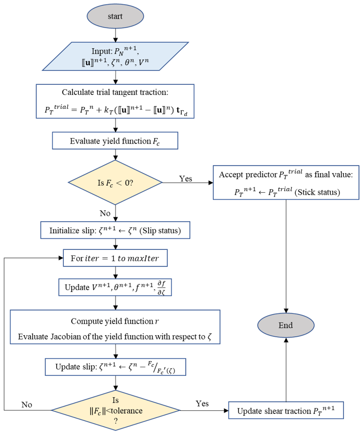
Figure 2 Flowchart of the predictor–corrector return-mapping algorithm used to update tangential traction and slip at the fault interface under rate-and-state friction. The procedure evaluates stick or slip conditions based on a yield criterion, with iterative correction of slip and frictional variables during the slip phase until convergence is achieved.

To enforce the active sliding condition, the nonlinear consistency equation $F_{\mathrm{c}}\left({\mathit{\zeta }}^{n+\mathrm{1}}\right)=\mathrm{0}$ is solved using a Newton–Raphson iteration. During this local update, the displacement jump is kept fixed, and the Jacobian is obtained by differentiating Eq. (15) with respect to the plastic slip variable ζ:

$$\begin{array}{}\text{(16)}& {\displaystyle \frac{\partial F_{\mathrm{c}}}{\partial \mathit{\zeta }}}=-k_{\mathrm{T}}+{\displaystyle \frac{\partial f^{n+\mathrm{1}}}{\partial \mathit{\zeta }}}{k}_{\mathrm{N}}\left[[\mathit{u}\right]]\cdot {\mathit{n}}_{{\mathrm{\Gamma }}_{\mathrm{d}}}\end{array}$$

At each iteration, the derivative of the friction coefficient with respect to the plastic slip must be evaluated. The friction coefficient evolves according to a rate-and-state formulation (Dieterich, 1979; Ruina, 1983), which is a phenomenological constitutive relation widely used to model velocity- and state-dependent fault friction:

$$\begin{array}{}\text{(17)}& f=f_{\mathrm{0}}+a\ln \left({\displaystyle \frac{V^{n+\mathrm{1}}}{V^{*}}}\right)+b\ln \left({\displaystyle \frac{{\mathit{\theta }}^{n+\mathrm{1}}}{{\mathit{\theta }}^{*}}}\right)\end{array}$$

where V^* denotes the reference slip velocity, while f₀ represents the steady-state friction coefficient. The state variable, θ, characterizes the dependence of friction on both slip time and slip history, whereas θ^* corresponds to its steady-state value when the fault interface is sliding at the reference velocity V^*. The direct effect and friction evolution are denoted by the parameters a and b, respectively. In this work, the evolution of the state variable is governed by the aging law (Dieterich, 1979; Ruina, 1983):

$$\begin{array}{}\text{(18)}& \dot{\mathit{\theta }}=\mathrm{1}-{\displaystyle \frac{V^{n+\mathrm{1}}{\mathit{\theta }}^{n+\mathrm{1}}}{D_{\mathrm{c}}}}\end{array}$$

where D_c is the characteristic slip distance. The aging law is commonly used in the Dieterich–Ruina rate-and-state friction framework to describe contact aging and frictional healing during quasi-stationary periods (Dieterich, 1979; Ruina, 1983). Applying a backward Euler discretization yields:

$$\begin{array}{}\text{(19)}& {\mathit{\theta }}^{n+\mathrm{1}}={\displaystyle \frac{{\mathit{\theta }}^n+\mathrm{\Delta }t}{\mathrm{1}+\frac{\mathrm{\Delta }t{V}^{n+\mathrm{1}}}{D_{\mathrm{c}}}}}\end{array}$$

The derivative of the friction coefficient with respect to slip is subsequently obtained using the chain rule:

$$\begin{array}{}\text{(20)}& \begin{array}{rl}{\displaystyle \frac{\partial f}{\partial \mathit{\zeta }}}& ={\displaystyle \frac{\partial f}{\partial V}}{\displaystyle \frac{\partial V}{\partial \mathit{\zeta }}}+{\displaystyle \frac{\partial f}{\partial \mathit{\theta }}}{\displaystyle \frac{\partial \mathit{\theta }}{\partial \mathit{\zeta }}}={\displaystyle \frac{\mathrm{1}}{\mathrm{\Delta }t}}\\ & \left({\displaystyle \frac{a}{V^{n+\mathrm{1}}}}-{\displaystyle \frac{b}{{\mathit{\theta }}^{n+\mathrm{1}}}}{\displaystyle \frac{D_{\mathrm{c}}\mathrm{\Delta }t({\mathit{\theta }}^n+\mathrm{\Delta }t)}{{\left(D_{\mathrm{c}}+\mathrm{\Delta }t{V}^{n+\mathrm{1}}\right)}^{\mathrm{2}}}}\right),\\ & V^{n+\mathrm{1}}={\displaystyle \frac{{\mathit{\zeta }}^{n+\mathrm{1}}-{\mathit{\zeta }}^n}{\mathrm{\Delta }t}}\end{array}\end{array}$$

The slip variable ζⁿ⁺¹ is iteratively updated until Eq. (15) is satisfied. At each iteration, the slip velocity, state variable, friction coefficient, and its derivative with respect to slip are updated accordingly. Upon convergence, the tangential traction and all internal variables are finalized, ensuring a consistent and physically sound representation of the interface response under evolving frictional conditions. It should be noted that the fault is represented as a one-dimensional interface with a single tangential slip direction; therefore, V is a scalar slip speed. For a higher-dimensional fault surface, the tangential slip velocity would generally be vector-valued, and the quantity V entering the rate-and-state friction law would correspond to the magnitude of that tangential slip-velocity vector.

2.4 Interpolation of pressure and displacement fields

Within the XFEM framework, the displacement field u(x,t) is approximated using an enriched formulation that augments the standard finite element interpolation with additional functions to represent displacement discontinuities and near-tip singularities (Dolbow et al., 2000). The resulting approximation is written as:

$$\begin{array}{}\text{(21)}& \begin{array}{rl}{\mathit{u}}^{\mathrm{e}}\left(\mathit{x},t\right)& =\sum _{i=\mathrm{1}}^{\mathcal{N}}{N}_{ui}\left(\mathit{x}\right){\stackrel{\mathrm{‾}}{\mathit{u}}}_{\mathrm{i}}\left(t\right)+\sum _{i=\mathrm{1}}^{{\mathcal{N}}^{\mathrm{Hev}}}{N}_{ui}\left(\mathit{x}\right)\left(H\left(\mathit{\phi }\left(\mathit{x}\right)\right)\right.\\ & \left.-H\left(\mathit{\phi }\left({\mathit{x}}_i\right)\right)\right){\mathit{a}}_{\mathrm{i}}\left(t\right)+\sum _{i=\mathrm{1}}^{{\mathcal{N}}^{\mathrm{tip}}}{N}_{ui}\left(\mathit{x}\right)\sum _{j=\mathrm{1}}^{\mathrm{4}}\left(T_j\left(\mathit{x}\right)\right.\\ & \left.-T_j\left({\mathit{x}}_i\right)\right){\stackrel{\mathrm{‾}}{\mathit{b}}}_{ji}\left(t\right)={\mathbf{N}}_u^{\mathrm{std}}\left(\mathit{x}\right)\stackrel{\mathrm{‾}}{\mathit{u}}\left(t\right)\\ & +{\mathbf{N}}_u^{\mathrm{Hev}}\left(\mathit{x}\right)\mathit{a}\left(t\right)+{\mathbf{N}}_u^{\mathrm{tip}}\left(\mathit{x}\right)\stackrel{\mathrm{‾}}{\mathit{b}}\left(t\right)\end{array}\end{array}$$

where 𝒩 denotes the number of all nodal points within element e, and 𝒩^Hev and 𝒩^tip represent the number of nodes enriched by the Heaviside function H(φ(x))−H(φ(x_i)) and crack-tip asymptotic functions $\sum _{j=\mathrm{1}}^{\mathrm{4}}\left(T_j\left(\mathit{x}\right)-T_j\left({\mathit{x}}_i\right)\right)$, respectively. Here, φ(x) denotes the signed distance function defining the crack geometry. The vectors ${\stackrel{\mathrm{‾}}{\mathit{u}}}_i\left(t\right)$, a_i(t), and ${\stackrel{\mathrm{‾}}{\mathit{b}}}_{ji}\left(t\right)$ correspond to the standard, Heaviside-enriched, and tip-enriched degrees of freedom. In this formulation, Heaviside enrichment means that the approximation space of nodes whose support is intersected by the crack is augmented by discontinuous basis functions of the form N_ui(x)(H(φ(x))−H(φ(x_i))), which introduces additional nodal degrees of freedom a_i(t). Since the Heaviside function takes different constant values on the two sides of the crack, this enrichment allows the displacement field to have two independent traces across the crack faces. Therefore, a displacement jump can be represented inside an element without requiring the finite element mesh to conform to the crack geometry. The shifted form H(φ(x))−H(φ(x_i)) is used to preserve the standard nodal interpolation property. In other words, the Heaviside enrichment enables the representation of strong discontinuities, where the displacement field itself is allowed to be discontinuous across the contact surface. The Heaviside function is given by

$$\begin{array}{}\text{(22)}& H\left(\mathit{\phi }\right(x\left)\right)=\left\{\begin{array}{cc}+\mathrm{1}& \mathit{\phi }\left(x\right)>\mathrm{0}\\ -\mathrm{1}& \mathit{\phi }\left(x\right)<\mathrm{0}\end{array}\right.\end{array}$$

In contrast, the crack-tip enrichment improves the approximation of the near-tip singular displacement field. The crack-tip enrichment functions are defined as (Moës et al., 1999):

$$\begin{array}{}\text{(23)}& \begin{array}{rl}& T(r,{\mathit{\beta }}_{\mathrm{f}})=\left\{T_{\mathrm{1}},T_{\mathrm{2}},T_{\mathrm{3}},T_{\mathrm{4}}\right\}=\\ & \left\{\sqrt{r}\sin {\displaystyle \frac{{\mathit{\beta }}_{\mathrm{f}}}{\mathrm{2}}},\sqrt{r}\cos {\displaystyle \frac{{\mathit{\beta }}_{\mathrm{f}}}{\mathrm{2}}},\sqrt{r}\sin {\displaystyle \frac{{\mathit{\beta }}_{\mathrm{f}}}{\mathrm{2}}}\sin \mathit{\theta },\sqrt{r}\cos {\displaystyle \frac{{\mathit{\beta }}_{\mathrm{f}}}{\mathrm{2}}}\sin \mathit{\theta }\right\}\end{array}\end{array}$$

where r is the distance from the crack tip, and β_f is the polar angle measured from the crack line. The displacement jump across the contact surface can be written as:

$$\begin{array}{}\text{(24)}& \begin{array}{rl}\left[[\mathit{u}\right]]& =\left[[{\mathbf{N}}_u^{\mathrm{std}}\left(\mathit{x}\right)\stackrel{\mathrm{‾}}{\mathit{u}}\left(t\right)+{\mathbf{N}}_u^{\mathrm{Hev}}\left(\mathit{x}\right)\mathit{a}\left(t\right)+{\mathbf{N}}_u^{\mathrm{tip}}\left(\mathit{x}\right)\stackrel{\mathrm{‾}}{\mathit{b}}\left(t\right)\right]]\\ & =\left[[{\mathbf{N}}_u^{\mathrm{std}}\left(\mathit{x}\right)\stackrel{\mathrm{‾}}{\mathit{u}}\left(t\right)\right]]+\left[[{\mathbf{N}}_u^{\mathrm{Hev}}\left(\mathit{x}\right)\mathit{a}\left(t\right)\right]]+\left[[{\mathbf{N}}_u^{\mathrm{tip}}\left(\mathit{x}\right)\stackrel{\mathrm{‾}}{\mathit{b}}\left(t\right)\right]]\end{array}\end{array}$$

The term involving the standard shape functions ${\mathbf{N}}_u^{\mathrm{std}}$ vanishes since these functions are continuous across the interface. Consequently, the displacement jump induced by the Heaviside and tip enrichment reduces to:

$$\begin{array}{}\text{(25)}& {\displaystyle }\left[[{\mathbf{N}}_u^{\mathrm{Hev}}\left(\mathit{x}\right)\mathit{a}\left(t\right)\right]]=\mathrm{2}\sum _{i=\mathrm{1}}^{{\mathcal{N}}^{\mathrm{Hev}}}{N}_{ui}\left(\mathit{x}\right){\mathit{a}}_i\left(t\right)\text{(26)}& {\displaystyle }\left[[{\mathbf{N}}_u^{\mathrm{tip}}\left(\mathit{x}\right)\stackrel{\mathrm{‾}}{\mathit{b}}\left(t\right)\right]]=\mathrm{2}\sum _{i=\mathrm{1}}^{{\mathcal{N}}^{\mathrm{tip}}}{N}_{ui}\left(\mathit{x}\right)\sqrt{r}{\stackrel{\mathrm{‾}}{\mathit{b}}}_{\mathrm{1}i}\left(t\right)\end{array}$$

Among the four crack-tip asymptotic enrichment functions, only the first function generates a displacement discontinuity across the crack faces (Khoei, 2015). The remaining functions primarily enhance the approximation quality in the vicinity of the crack tip and therefore do not contribute to the jump. Based on the XFEM displacement enrichment, the strain field is decomposed into standard, discontinuous, and crack-tip contributions. Accordingly, the strain at position x and time t can be written as:

$$\begin{array}{}\text{(27)}& {\mathit{ϵ}}^{\mathrm{e}}\left(\mathit{x},t\right)={\mathbf{B}}^{\mathrm{std}}\left(\mathit{x}\right)\stackrel{\mathrm{‾}}{\mathit{u}}\left(t\right)+{\mathbf{B}}^{\mathrm{Hev}}\left(\mathit{x}\right)\mathit{a}\left(t\right)+{\mathbf{B}}^{\mathrm{tip}}\left(\mathit{x}\right)\stackrel{\mathrm{‾}}{\mathit{b}}\left(t\right)\end{array}$$

where B^std is spatial derivatives of standard shape functions, and B^Hev and B^tip are spatial derivatives of enriched shape functions associated with Heaviside enrichment function and crack-tip asymptotic functions, respectively. The evaluation of the spatial derivatives of the crack-tip enrichment functions requires a transformation from the local crack-tip polar coordinate system to the global Cartesian coordinates (x,y) (Khoei, 2015). This transformation can be expressed as:

$$\begin{array}{}\text{(28)}& \mathrm{\nabla }{T}_j=\mathbf{R}\left({\mathit{\beta }}_{\mathrm{f}}\right)\mathrm{\nabla }{}^{\prime }{T}_j=\mathbf{R}\left({\mathit{\beta }}_{\mathrm{f}}\right){\mathbf{J}}_{\mathrm{r}{\mathit{\beta }}_{\mathrm{f}}}\left[\begin{array}{c}{T}_{j,r}\\ T_{j,{\mathit{\beta }}_{\mathrm{f}}}\end{array}\right]\end{array}$$

where R is rotation matrix with β_f denoting the angle between the local crack-tip coordinate system $\left(x{}^{\prime },y{}^{\prime }\right)$ and the global coordinate axes (x,y), and ${\mathbf{J}}_{\mathrm{r}{\mathit{\beta }}_{\mathrm{f}}}$ is the Jacobian relating polar coordinates (r,β_f) to the local Cartesian coordinates.

The enriched approximation of the XFEM for the pressure field p(x,t) can be written as:

$$\begin{array}{}\text{(29)}& \begin{array}{rl}{p}^{\mathrm{e}}\left(\mathit{x},t\right)& =\sum _{i=\mathrm{1}}^{\mathcal{N}}{N}_{p_i}\left(\mathit{x}\right){\stackrel{\mathrm{‾}}{p}}_i\left(t\right)+\sum _{i=\mathrm{1}}^{{\mathcal{N}}^{\mathrm{mod}}}{N}_{p_i}\left(\mathit{x}\right)\left(\mathrm{\Psi }\left(\mathit{x}\right)\right.\\ & \left.-\mathrm{\Psi }\left({\mathit{x}}_i\right)\right){\stackrel{\mathrm{‾}}{d}}_i\left(t\right)={\mathbf{N}}_{\mathrm{p}}^{\mathrm{std}}\left(\mathit{x}\right)\stackrel{\mathrm{‾}}{\mathit{p}}\left(\mathrm{t}\right)+{\mathbf{N}}_{\mathrm{p}}^{\mathrm{mod}}\left(\mathit{x}\right)\stackrel{\mathrm{‾}}{\mathit{d}}\left(\mathrm{t}\right)\end{array}\end{array}$$

where 𝒩^mod represents the number of nodes enriched by the modified level-set function Ψ(x)−Ψ(x_i), ${\stackrel{\mathrm{‾}}{p}}_i\left(t\right)$ denotes the nodal pressure degrees of freedom associated with the standard interpolation, whereas ${\stackrel{\mathrm{‾}}{d}}_i\left(t\right)$ denote the additional enriched pressure degrees of freedom introduced to capture non-smooth pressure variations near the interface. The matrix ${\mathbf{N}}_p^{\mathrm{mod}}$ collects the enriched pressure shape functions with ith entry of $N_{p_i}\left(\mathit{x}\right)\left(\mathrm{\Psi }\left(\mathit{x}\right)-\mathrm{\Psi }\left({\mathit{x}}_i\right)\right)$. The shifted form Ψ(x)−Ψ(x_i) ensures that the enriched contribution vanishes at the enriched node x_i, thereby preserving the standard nodal pressure interpolation. In this study, the modified level-set function is defined following Fries and Belytschko (2010) as:

$$\begin{array}{}\text{(30)}& \mathrm{\Psi }\left(\mathit{x}\right)=\sum _{i=\mathrm{1}}^{{\mathcal{N}}^{\mathrm{mod}}}{N}_{p_i}\left(\mathit{x}\right)\left|\mathit{\phi }\left({\mathit{x}}_i\right)\right|-\left|\sum _{i=\mathrm{1}}^{{\mathcal{N}}^{\mathrm{mod}}}{N}_{pi}\left(\mathit{x}\right)\mathit{\phi }\left({\mathit{x}}_i\right)\right|\end{array}$$

This formulation produces an enrichment function that forms a ridge aligned with the interface. As a result, the pressure field remains continuous across the interface, while its spatial gradient is allowed to exhibit a jump. An additional advantage of this construction is that the enrichment naturally vanishes in elements that are not intersected by the interface, thereby eliminating the need for special blending treatments. The pressure gradient inside an enriched element can therefore be evaluated as:

$$\begin{array}{}\text{(31)}& \begin{array}{rl}& \mathrm{\nabla }{p}^{\mathrm{e}}\left(\mathit{x},t\right)=\sum _{i=\mathrm{1}}^{\mathcal{N}}\mathrm{\nabla }{N}_{p_i}\left(\mathit{x}\right){\stackrel{\mathrm{‾}}{p}}_i\left(t\right)+\sum _{i=\mathrm{1}}^{{\mathcal{N}}^{\mathrm{mod}}}\\ & \left[\mathrm{\nabla }{N}_{p_i}\left(\mathit{x}\right)\left(\mathrm{\Psi }\left(\mathit{x}\right)-\mathrm{\Psi }\left({\mathit{x}}_i\right)\right)+N_{p_i}\left(\mathit{x}\right)\mathrm{\nabla }\mathrm{\Psi }\left(\mathit{x}\right)\right]{\stackrel{\mathrm{‾}}{d}}_i\left(t\right)\end{array}\end{array}$$

The gradient of the modified level set function Ψ(x) is computed as follows:

$$\begin{array}{}\text{(32)}& \begin{array}{rl}\mathrm{\nabla }\mathrm{\Psi }\left(\mathit{x}\right)& =\sum _{i=\mathrm{1}}^{{\mathcal{N}}^{\mathrm{mod}}}\mathrm{\nabla }{N}_{p_i}\left(\mathit{x}\right)\left|\mathit{\phi }\left({\mathit{x}}_i\right)\right|-\mathrm{sgn}\\ & \left(\sum _{i=\mathrm{1}}^{{\mathcal{N}}^{\mathrm{mod}}}{N}_{pi}\left(\mathit{x}\right)\mathit{\phi }\left({\mathit{x}}_i\right)\right)\sum _{i=\mathrm{1}}^{{\mathcal{N}}^{\mathrm{mod}}}\mathrm{\nabla }{N}_{p_i}\left(\mathit{x}\right)\mathit{\phi }\left({\mathit{x}}_i\right)\end{array}\end{array}$$

2.5 The XFEM spatial and temporal discretization

By introducing the enriched trial functions for the displacement field (Eq. 21) and the pressure field (Eq. 29), together with their corresponding test functions, and substituting them into the weak formulations given in Eqs. (4) and (5), as well as the relevant interface integral relations, the governing equations can be rearranged into a global matrix form, leading to the following semi-discrete system governing the displacement field:

$$\begin{array}{}\text{(33)}& \begin{array}{rl}& {\mathbf{M}}_{l\times l}{\ddot{\mathit{U}}}_{l\times \mathrm{1}}+{\mathbf{D}}_{l\times l}{\dot{\mathit{U}}}_{l\times \mathrm{1}}+{\mathbf{K}}_{l\times l}{\mathit{U}}_{l\times \mathrm{1}}-{\mathbf{Q}}_{l\times p}{\mathit{P}}_{p\times \mathrm{1}}\\ & +{\mathit{F}}_{\mathrm{int}}-{\mathit{F}}_{\mathrm{ext}}=\mathrm{0}\end{array}\end{array}$$

where l denotes the total number of degrees of freedom (DOFs) for displacement, and p is the total number of DOFs associated with pressure. In this formulation, M represents the global mass matrix, D the damping matrix, K the global stiffness matrix, and Q the coupling matrix linking displacement field U to pressure P field. The vectors F_ext and F_int represent the external and internal force vectors, respectively. The individual matrices are defined as follows:

$$\begin{array}{}\text{(34)}& \begin{array}{rl}& \mathbf{M}={\int }_{\mathrm{\Omega }}{\left({\mathbf{N}}_u\right)}^T\mathit{\rho }{\mathbf{N}}_u\mathrm{d}\mathrm{\Omega }\\ & \mathbf{K}={\int }_{\mathrm{\Omega }}{{\mathbf{B}}_u}^T\mathbb{C}{\mathbf{B}}_u\mathrm{d}\mathrm{\Omega }\\ & \mathbf{D}=a_{\mathrm{Ray}}\mathbf{M}+b_{\mathrm{Ray}}\mathbf{K}+{\int }_{{\mathrm{\Gamma }}_{\mathrm{abs}}}{{\mathbf{N}}_u}^T\mathit{\rho }{\mathbf{VN}}_u\mathrm{d}\mathrm{\Gamma }\\ & \mathbf{Q}={\int }_{\mathrm{\Omega }}{{\mathbf{B}}_u}^T\mathit{\alpha }\mathit{m}{\mathbf{N}}_p\mathrm{d}\mathrm{\Omega }+{\int }_{{\mathrm{\Gamma }}_{\mathrm{d}}}\left[[{\mathbf{N}}_u\right]{]}^T\cdot {\mathit{n}}_{{\mathrm{\Gamma }}_{\mathrm{d}}}{\mathbf{N}}_p\mathrm{d}\mathrm{\Gamma }\\ & {\mathit{F}}_{\mathrm{ext}}={\int }_{\mathrm{\Omega }}{\left({\mathbf{N}}_u\right)}^T\mathit{\rho }\mathit{b}\mathrm{d}\mathrm{\Omega }+{\int }_{{\mathrm{\Gamma }}_t}{\left({\mathbf{N}}_u\right)}^T\stackrel{\mathrm{‾}}{\mathit{t}}\mathrm{d}\mathrm{\Gamma }\\ & {\mathit{F}}_{\mathrm{int}}={\int }_{{\stackrel{\mathrm{̃}}{\mathrm{\Gamma }}}_{\mathrm{d}}}\left[[{\mathbf{N}}_u\right]{]}^T\left(P_{\mathrm{N}}{\mathit{n}}_{{\mathrm{\Gamma }}_{\mathrm{d}}}+P_{\mathrm{T}}{\mathit{t}}_{{\mathrm{\Gamma }}_{\mathrm{d}}}\right)\mathrm{d}\mathrm{\Gamma }\end{array}\end{array}$$

where ℂ is the fourth-order elastic constitutive tensor and Γ_abs denotes the absorbing portion of the boundary. The global damping matrix D comprises two contributions: Rayleigh damping and the Lysmer–Kuhlemeyer absorbing boundary formulation. Rayleigh damping is introduced at the semi-discrete level as a linear combination of the global mass and stiffness matrices to control spurious oscillatory responses (Liu and Gorman, 1995), whereas the Lysmer–Kuhlemeyer formulation is applied at the external boundaries to minimize artificial wave reflections (Lysmer and Kuhlemeyer, 1969). Material viscosity is therefore not introduced explicitly through the continuous constitutive relation; instead, energy dissipation is represented after XFEM spatial discretization through the Rayleigh damping matrix. In this formulation, a_Ray and b_Ray denote the mass- and stiffness-proportional Rayleigh damping coefficients, respectively. These coefficients are determined by prescribing a target damping ratio of ξ=0.04 at two selected natural angular frequencies, ω₁ and ω₃, and are defined as (Kontoe et al., 2011):

$$\begin{array}{}\text{(35)}& a_{\mathrm{Ray}}={\displaystyle \frac{\mathrm{2}{\mathit{\omega }}_{\mathrm{1}}{\mathit{\omega }}_{\mathrm{3}}\mathit{\xi }}{{\mathit{\omega }}_{\mathrm{1}}+{\mathit{\omega }}_{\mathrm{3}}}},b_{\mathrm{Ray}}={\displaystyle \frac{\mathrm{2}\mathit{\xi }}{{\mathit{\omega }}_{\mathrm{1}}+{\mathit{\omega }}_{\mathrm{3}}}}\end{array}$$

In the second term in damping matrix, the parameter $\stackrel{\mathrm{‾}}{\mathit{\rho }}$ denotes the spatially averaged density of the mixture, and V is a wave-speed matrix defined as:

$$\begin{array}{}\text{(36)}& \mathbf{V}=\left\{\begin{array}{cc}\left[\begin{array}{cc}{a}_{\mathrm{p}}{\stackrel{\mathrm{‾}}{V}}_{\mathrm{p}}& \mathrm{0}\\ \mathrm{0}& a_{\mathrm{s}}{\stackrel{\mathrm{‾}}{V}}_{\mathrm{s}}\end{array}\right],& \mathrm{if}{\mathit{n}}_{\mathrm{\Gamma }}\mathrm{\Vert }x\\ \left[\begin{array}{cc}{a}_{\mathrm{s}}{\stackrel{\mathrm{‾}}{V}}_{\mathrm{s}}& \mathrm{0}\\ \mathrm{0}& a_{\mathrm{p}}{\stackrel{\mathrm{‾}}{V}}_{\mathrm{p}}\end{array}\right],& \mathrm{if}{\mathit{n}}_{\mathrm{\Gamma }}\mathrm{\Vert }y\end{array}\right.\end{array}$$

where a_p and a_s are scaling coefficients, here both taken equal to unity, and ${\stackrel{\mathrm{‾}}{V}}_{\mathrm{p}}$ and ${\stackrel{\mathrm{‾}}{V}}_{\mathrm{s}}$ are the average compressional and shear velocities. For the pressure field, the semi-discrete governing equation can be written as:

$$\begin{array}{}\text{(37)}& \begin{array}{rl}& {\mathbf{C}}_{p\times l}{\ddot{\mathit{U}}}_{l\times \mathrm{1}}+{{\mathbf{Q}}^p}_{p\times l}{\dot{\mathit{U}}}_{l\times \mathrm{1}}+{\mathbf{H}}_{p\times p}{\mathit{P}}_{p\times \mathrm{1}}+{\mathbf{S}}_{p\times p}{\dot{\mathit{P}}}_{p\times \mathrm{1}}\\ & -{\mathit{q}}_{\mathrm{ext}}=\mathrm{0}\end{array}\end{array}$$

where C represents the inertial coupling between the fluid and the solid skeleton, H is the hydraulic conductivity matrix, S denotes the storage matrix, and q_ext is an external source term. These matrices are defined as follows:

$$\begin{array}{}\text{(38)}& \begin{array}{rl}& \mathbf{C}={\int }_{\mathrm{\Omega }}{\left(\mathrm{\nabla }{\mathbf{N}}_p\right)}^T\mathit{k}{\mathit{\rho }}_{\mathrm{f}}{\mathbf{N}}_u\mathrm{d}\mathrm{\Omega }+{\int }_{{\mathrm{\Gamma }}_{\mathrm{d}}}{\left(\mathrm{\nabla }{\mathbf{N}}_p\right)}^T\\ & \cdot {\mathit{t}}_{{\mathrm{\Gamma }}_{\mathrm{d}}}\left({\displaystyle \frac{w^{\mathrm{3}}}{\mathrm{12}{\mathit{\mu }}_{\mathrm{f}}}}{\mathit{\rho }}_{\mathrm{f}}\right)〈{\mathbf{N}}_u〉\cdot {\mathit{t}}_{{\mathrm{\Gamma }}_{\mathrm{d}}}\mathrm{d}\mathrm{\Gamma }\\ & \mathbf{H}={\int }_{\mathrm{\Omega }}{\left(\mathrm{\nabla }{\mathbf{N}}_p\right)}^T\mathit{k}\left(\mathrm{\nabla }{\mathbf{N}}_p\right)\mathrm{d}\mathrm{\Omega }+{\int }_{{\mathrm{\Gamma }}_{\mathrm{d}}}{\left(\mathrm{\nabla }{\mathbf{N}}_p\right)}^T\\ & \cdot {\mathit{t}}_{{\mathrm{\Gamma }}_{\mathrm{d}}}\left({\displaystyle \frac{w^{\mathrm{3}}}{\mathrm{12}{\mathit{\mu }}_{\mathrm{f}}}}\right)\left(\mathrm{\nabla }{\mathbf{N}}_p\right)\cdot {\mathit{t}}_{{\mathrm{\Gamma }}_{\mathrm{d}}}\mathrm{d}\mathrm{\Gamma }\\ & \mathbf{S}={\int }_{\mathrm{\Omega }}{\left({\mathbf{N}}_p\right)}^T{S}_{\mathrm{s}}{\mathbf{N}}_p\mathrm{d}\mathrm{\Omega }+{\int }_{{\mathrm{\Gamma }}_{\mathrm{d}}}{\left({\mathbf{N}}_p\right)}^{T}w{C}_{\mathrm{f}}{\mathbf{N}}_p\mathrm{d}\mathrm{\Gamma }\\ & {\mathbf{Q}}^p={\mathbf{Q}}^T+{\int }_{{\mathrm{\Gamma }}_{\mathrm{d}}}{\left({\mathbf{N}}_p\right)}^{T}w{\mathit{t}}_{{\mathrm{\Gamma }}_{\mathrm{d}}}\cdot 〈\mathrm{\nabla }{\mathbf{N}}_u〉\cdot {\mathit{t}}_{{\mathrm{\Gamma }}_{\mathrm{d}}}\mathrm{d}\mathrm{\Gamma }\\ & {\mathit{q}}_{\mathrm{ext}}={\int }_{\mathrm{\Omega }}{\left(\mathrm{\nabla }{\mathbf{N}}_p\right)}^T\mathit{k}{\mathit{\rho }}_{\mathrm{f}}\mathit{b}\mathrm{d}\mathrm{\Omega }-{\int }_{{\mathrm{\Gamma }}_{\mathrm{w}}}{\left({\mathbf{N}}_p\right)}^T\stackrel{\mathrm{‾}}{q}\mathrm{d}\mathrm{\Gamma }\\ & -{\int }_{{\mathrm{\Gamma }}_{\mathrm{d}}}{\left(\mathrm{\nabla }{\mathbf{N}}_p\right)}^T\cdot {\mathit{t}}_{{\mathrm{\Gamma }}_{\mathrm{d}}}\left({\displaystyle \frac{w^{\mathrm{3}}}{\mathrm{12}{\mathit{\mu }}_{\mathrm{f}}}}{\mathit{\rho }}_{\mathrm{f}}\right)\mathit{b}\cdot {\mathit{t}}_{{\mathrm{\Gamma }}_{\mathrm{d}}}\mathrm{d}\mathrm{\Gamma }\end{array}\end{array}$$

2.5.1 Fully implicit time integration strategy

The semi-discrete XFEM governing equations are first integrated in time using a fully implicit solution strategy, which serves as the reference formulation throughout this work. Displacement is advanced with a generalized Newmark GN22 method, while pressure is updated using a GN11 scheme. The unknown fields at time $t_{n+\mathrm{1}}=t_n+\mathrm{\Delta }t$ are related to known values at t_n through the following formulas:

$$\begin{array}{}\text{(39)}& \begin{array}{rl}& {\ddot{\mathit{U}}}_{n+\mathrm{1}}={\displaystyle \frac{\mathrm{1}}{\mathit{\beta }\mathrm{\Delta }{t}^{\mathrm{2}}}}\left({\mathit{U}}_{n+\mathrm{1}}-{\mathit{U}}_n\right)-{\displaystyle \frac{\mathrm{1}}{\mathit{\beta }\mathrm{\Delta }t}}{\dot{\mathit{U}}}_n-\left({\displaystyle \frac{\mathrm{1}}{\mathrm{2}\mathit{\beta }}}-\mathrm{1}\right){\ddot{\mathit{U}}}_n\\ & {\dot{\mathit{U}}}_{n+\mathrm{1}}={\displaystyle \frac{\mathit{\gamma }}{\mathit{\beta }\mathrm{\Delta }t}}\left({\mathit{U}}_{n+\mathrm{1}}-{\mathit{U}}_n\right)-\left({\displaystyle \frac{\mathit{\gamma }}{\mathit{\beta }}}-\mathrm{1}\right){\dot{\mathit{U}}}_n-\mathrm{\Delta }t\left({\displaystyle \frac{\mathit{\gamma }}{\mathrm{2}\mathit{\beta }}}-\mathrm{1}\right){\ddot{\mathit{U}}}_n\\ & {\dot{\mathit{P}}}_{n+\mathrm{1}}={\displaystyle \frac{\mathrm{1}}{\mathrm{\Delta }t}}\left({\mathit{P}}_{n+\mathrm{1}}-{\mathit{P}}_n\right)\end{array}\end{array}$$

This temporal discretization approach provides stable and accurate integration of second-order and first-order time-dependent equations, respectively. Unconditional stability of the displacement integration is ensured by selecting Newmark parameters satisfying $\mathit{\gamma }\ge \mathrm{0.5},\mathit{\beta }\ge \mathrm{0.25}(\mathrm{0.5}+\mathit{\gamma }{)}^{\mathrm{2}}$. In this work, the constant-average-acceleration scheme is employed with γ=0.5 and β=0.25 (Newmark, 1959). The vectors U_n, ${\dot{\mathit{U}}}_n$, and ${\ddot{\mathit{U}}}_n$ denote the displacement, velocity, and acceleration fields – including both standard and enriched degrees of freedom – at time step n, while P_n represents the corresponding pressure field. Substitution of the time discretization into the semi-discrete equations yields a fully discrete nonlinear system at n+1. The residual form of the coupled system is written as:

$$\begin{array}{}\text{(40)}& {\displaystyle }\begin{array}{rl}& {\mathit{R}}_{U_{n+\mathrm{1}}}=\left({\displaystyle \frac{\mathrm{1}}{\mathit{\beta }\mathrm{\Delta }{t}^{\mathrm{2}}}}\mathbf{M}+{\displaystyle \frac{\mathit{\gamma }}{\mathit{\beta }\mathrm{\Delta }t}}\mathbf{D}+\mathbf{K}\right){\mathit{U}}_{n+\mathrm{1}}-\mathbf{Q}{\mathit{P}}_{n+\mathrm{1}}\\ & -\left({\displaystyle \frac{\mathrm{1}}{\mathit{\beta }\mathrm{\Delta }{t}^{\mathrm{2}}}}\mathbf{M}+{\displaystyle \frac{\mathit{\gamma }}{\mathit{\beta }\mathrm{\Delta }t}}\mathbf{D}\right){\mathit{U}}_n-\left({\displaystyle \frac{\mathrm{1}}{\mathit{\beta }\mathrm{\Delta }t}}\mathbf{M}+\left({\displaystyle \frac{\mathit{\gamma }}{\mathit{\beta }}}-\mathrm{1}\right)\mathbf{D}\right){\dot{\mathit{U}}}_n\\ & -\left(\left({\displaystyle \frac{\mathrm{1}}{\mathrm{2}\mathit{\beta }}}-\mathrm{1}\right)\mathbf{M}+\mathrm{\Delta }t\left({\displaystyle \frac{\mathit{\gamma }}{\mathrm{2}\mathit{\beta }}}-\mathrm{1}\right)\mathbf{D}\right){\ddot{\mathit{U}}}_n+{\mathit{F}}_{\mathrm{int}}-{\mathit{F}}_{\mathrm{ext}}=\mathrm{0}\end{array}\text{(41)}& {\displaystyle }\begin{array}{rl}& {\mathit{R}}_{P_{n+\mathrm{1}}}=\left({\displaystyle \frac{\mathrm{1}}{\mathit{\beta }\mathrm{\Delta }{t}^{\mathrm{2}}}}\mathbf{C}+{\displaystyle \frac{\mathit{\gamma }}{\mathit{\beta }\mathrm{\Delta }t}}{{\mathbf{Q}}^p}_{n+\mathrm{1}}\right){\mathit{U}}_{n+\mathrm{1}}\\ & +\left({\mathbf{H}}_{n+\mathrm{1}}+{\displaystyle \frac{\mathrm{1}}{\mathrm{\Delta }t}}{\mathbf{S}}_{n+\mathrm{1}}\right){\mathit{P}}_{n+\mathrm{1}}-\left({\displaystyle \frac{\mathrm{1}}{\mathrm{\Delta }t}}{\mathbf{S}}_{n+\mathrm{1}}\right){\mathit{P}}_n\\ & -\left({\displaystyle \frac{\mathrm{1}}{\mathit{\beta }\mathrm{\Delta }{t}^{\mathrm{2}}}}\mathbf{C}+{\displaystyle \frac{\mathit{\gamma }}{\mathit{\beta }\mathrm{\Delta }t}}{{\mathbf{Q}}^p}_{n+\mathrm{1}}\right){\mathit{U}}_n\\ & -\left({\displaystyle \frac{\mathrm{1}}{\mathit{\beta }\mathrm{\Delta }t}}\mathbf{C}+\left({\displaystyle \frac{\mathit{\gamma }}{\mathit{\beta }}}-\mathrm{1}\right){{\mathbf{Q}}^p}_{n+\mathrm{1}}\right){\dot{\mathit{U}}}_n\\ & -\left(\left({\displaystyle \frac{\mathrm{1}}{\mathrm{2}\mathit{\beta }}}-\mathrm{1}\right)\mathbf{C}+\mathrm{\Delta }t\left({\displaystyle \frac{\mathit{\gamma }}{\mathrm{2}\mathit{\beta }}}-\mathrm{1}\right){{\mathbf{Q}}^p}_{n+\mathrm{1}}\right){\ddot{\mathit{U}}}_n-{\mathit{q}}_{\mathrm{ext}}=\mathrm{0}\end{array}\end{array}$$

The resulting coupled nonlinear system is solved using a fully monolithic Newton–Raphson approach, in which displacement and pressure unknowns are updated simultaneously at each time step. At iteration k of time step n+1, the residual equations are linearized about the current solution estimate, leading to the following incremental system:

$$\begin{array}{}\text{(42)}& \mathbf{J}\left({{\mathit{U}}_{n+\mathrm{1}}}^k,{{\mathit{P}}_{n+\mathrm{1}}}^k\right)\left\{\begin{array}{c}\mathit{\delta }{{\mathit{U}}_{n+\mathrm{1}}}^{k+\mathrm{1}}\\ \mathit{\delta }{{\mathit{P}}_{n+\mathrm{1}}}^{k+\mathrm{1}}\end{array}\right\}=-\left\{\begin{array}{c}{{\mathit{R}}_{U_{n+\mathrm{1}}}}^k\\ {{\mathit{R}}_{P_{n+\mathrm{1}}}}^k\end{array}\right\}\end{array}$$

where J is the Jacobian matrix evaluated at the current iteration. The Jacobian has a block structure and is given by:

$$\begin{array}{}\text{(43)}& \begin{array}{rl}& \mathbf{J}\left({{\mathit{U}}_{n+\mathrm{1}}}^k,{{\mathit{P}}_{n+\mathrm{1}}}^k\right)=\left[\begin{array}{cc}\frac{\partial {{\mathit{R}}_{U_{n+\mathrm{1}}}}^k}{\partial \mathit{U}}& \frac{\partial {{\mathit{R}}_{U_{n+\mathrm{1}}}}^k}{\partial \mathbf{P}}\\ \frac{\partial {{\mathit{R}}_{P_{n+\mathrm{1}}}}^k}{\partial \mathit{U}}& \frac{\partial {{\mathit{R}}_{P_{n+\mathrm{1}}}}^k}{\partial \mathbf{P}}\end{array}\right]\\ & =\left[\begin{array}{cc}\frac{\mathrm{1}}{\mathit{\beta }\mathrm{\Delta }{t}^{\mathrm{2}}}\mathbf{M}+\frac{\mathit{\gamma }}{\mathit{\beta }\mathrm{\Delta }t}\mathbf{D}+\mathbf{K}+\frac{\partial {\mathit{F}}_{\mathrm{int}}}{\partial \mathit{U}}& -\mathbf{Q}\\ \frac{\mathrm{1}}{\mathit{\beta }\mathrm{\Delta }{t}^{\mathrm{2}}}\mathbf{C}+\frac{\mathit{\gamma }}{\mathit{\beta }\mathrm{\Delta }t}{{\mathbf{Q}}^p}_{n+\mathrm{1}}& {\mathbf{H}}_{n+\mathrm{1}}+\frac{\mathrm{1}}{\mathrm{\Delta }t}{\mathbf{S}}_{n+\mathrm{1}}\end{array}\right]\end{array}\end{array}$$

Equation (43) represents the Jacobian blocks associated with the time-discretized governing equations when the coefficient matrices are held fixed during differentiation. However, in the present formulation, the hydraulic matrices C, H, S, and Q^p, together with the relevant source terms, depend on the evolving hydraulic aperture and consequently on the displacement field. As discussed in Sect. 2.6, these matrices are updated according to the current fault aperture during the Newton–Raphson iterations. Due to the hydro-mechanical coupling terms and the time discretization, the Jacobian matrix is generally non-symmetric. This non-symmetry can increase both memory requirements and computational cost. To improve the algebraic scaling of the coupled system, the rows associated with the displacement equations are multiplied by the non-zero factor $\frac{-\mathit{\gamma }}{\mathit{\beta }\mathrm{\Delta }t}$. This row scaling yields an algebraically equivalent linearized system, since it does not change the solution vector. Therefore, the scaled Jacobian should still be regarded as a non-symmetric matrix:

$$\begin{array}{}\text{(44)}& \begin{array}{rl}& \mathbf{J}\left({{\mathit{U}}_{n+\mathrm{1}}}^k,{{\mathit{P}}_{n+\mathrm{1}}}^k\right)=\\ & \left[\begin{array}{cc}\frac{-\mathit{\gamma }}{\mathit{\beta }\mathrm{\Delta }t}\left(\frac{\mathrm{1}}{\mathit{\beta }\mathrm{\Delta }{t}^{\mathrm{2}}}\mathbf{M}+\frac{\mathit{\gamma }}{\mathit{\beta }\mathrm{\Delta }t}\mathbf{D}+\mathbf{K}+\frac{\partial {\mathit{F}}_{\mathrm{int}}}{\partial \mathit{U}}\right)& \frac{\mathit{\gamma }}{\mathit{\beta }\mathrm{\Delta }t}\mathbf{Q}\\ \frac{\mathrm{1}}{\mathit{\beta }\mathrm{\Delta }{t}^{\mathrm{2}}}\mathbf{C}+\frac{\mathit{\gamma }}{\mathit{\beta }\mathrm{\Delta }t}{{\mathbf{Q}}^p}_{n+\mathrm{1}}& {\mathbf{H}}_{n+\mathrm{1}}+\frac{\mathrm{1}}{\mathrm{\Delta }t}{\mathbf{S}}_{n+\mathrm{1}}\end{array}\right]\end{array}\end{array}$$

The contribution of the interface to the Jacobian matrix arises from the dependence of the internal force vector on displacement discontinuities. Its linearization with respect to the displacement field is expressed as:

$$\begin{array}{}\text{(45)}& {\displaystyle \frac{\partial {\mathit{F}}_{\mathrm{int}}}{\partial U}}={\int }_{\stackrel{\mathrm{̃}}{{\mathrm{\Gamma }}_{\mathrm{d}}}}\left[[{\mathbf{N}}_u\right]{]}^T\mathbf{E}\left[[{\mathbf{N}}_u\right]]\mathrm{d}\mathrm{\Gamma }\end{array}$$

where E denotes the algorithmic (consistent) tangent operator associated with the fault constitutive response. At the current time step and Newton iteration, it is defined as the derivative of the algorithmically updated interface traction with respect to the displacement jump across the interface:

$$\begin{array}{}\text{(46)}& \mathbf{E}={\displaystyle \frac{\partial \left(\mathit{t}\right)}{\partial \left[[\mathit{u}\right]]}}={\displaystyle \frac{\partial \left(P_{\mathrm{N}}{\mathit{n}}_{{\mathrm{\Gamma }}_{\mathrm{d}}}+P_{\mathrm{T}}{\mathit{t}}_{{\mathrm{\Gamma }}_{\mathrm{d}}}\right)}{\partial \left[[\mathit{u}\right]]}}\end{array}$$

In fact, E represents the tangent stiffness of the time-discrete interface constitutive update, including the effects of contact stiffness, frictional slip, and the relevant internal state variables. The tangent operator is called consistent when it is obtained by differentiating the same discrete update equations used to compute the residual traction. In this case, E provides the exact linearization of the interface contribution entering the Newton residual, for a fixed active regime of the fault. This improves the robustness and convergence rate of the Newton–Raphson iterations. Since the interface response may change between stick and slip, E is evaluated according to the current active fault regime. In the stick regime, the corresponding tangent operator associated with fault-plane plasticity is given by:

$$\begin{array}{}\text{(47)}& \begin{array}{rl}{\mathbf{E}}^{\mathrm{stick}}& ={\mathit{n}}_{{\mathrm{\Gamma }}_{\mathrm{d}}}\otimes {\displaystyle \frac{\partial P_{\mathrm{N}}}{\partial \left[[\mathit{u}\right]]}}+{\mathit{t}}_{{\mathrm{\Gamma }}_{\mathrm{d}}}\otimes {\displaystyle \frac{\partial P_{\mathrm{T}}}{\partial \left[[\mathit{u}\right]]}}\\ & =k_{\mathrm{N}}\left({\mathit{n}}_{{\mathrm{\Gamma }}_{\mathrm{d}}}\otimes {\mathit{n}}_{{\mathrm{\Gamma }}_{\mathrm{d}}}\right)+k_{\mathrm{T}}(\mathbf{I}-{\mathit{n}}_{{\mathrm{\Gamma }}_{\mathrm{d}}}\otimes {\mathit{n}}_{{\mathrm{\Gamma }}_{\mathrm{d}}})\end{array}\end{array}$$

This expression reflects the linear elastic resistance to tangential motion during the stick phase, where the amount of plastic slip is zero $({\mathit{\zeta }}^{n+\mathrm{1}}={\mathit{\zeta }}^n)$. Under slipping conditions (${\mathit{\zeta }}^{n+\mathrm{1}}\ne {\mathit{\zeta }}^n$), the tangential traction, P_T, is governed by a rate-dependent frictional constitutive law. In this case, the linearization of the tangential traction with respect to the displacement jump is required to construct a consistent Jacobian contribution. Under slipping conditions, the derivative of the tangential traction magnitude with respect to the displacement discontinuity is given by:

$$\begin{array}{}\text{(48)}& {\displaystyle \frac{\partial P_{\mathrm{T}}}{\partial \left[[\mathit{u}\right]]}}=k_{\mathrm{T}}\left({\mathit{t}}_{{\mathrm{\Gamma }}_{\mathrm{d}}}-\mathrm{sgn}\left(P_{\mathrm{T}}\right){\displaystyle \frac{\partial \mathit{\zeta }}{\partial \left[[\mathit{u}\right]]}}\right)\end{array}$$

At a locally converged stress state, the derivative of ζ with respect to the displacement jump can be expressed as (Liu and Borja, 2009):

$$\begin{array}{}\text{(49)}& {\displaystyle \frac{\partial \mathit{\zeta }}{\partial \left[[\mathit{u}\right]]}}={\displaystyle \frac{\mathrm{sgn}\left(P_{\mathrm{T}}\right)k_{\mathrm{T}}{\mathit{t}}_{{\mathrm{\Gamma }}_{\mathrm{d}}}+k_{\mathrm{N}}{f}^{n+\mathrm{1}}{\mathit{n}}_{{\mathrm{\Gamma }}_{\mathrm{d}}}}{k_{\mathrm{T}}-\frac{\partial f}{\partial \mathit{\zeta }}{k}_{\mathrm{N}}\left[[\mathit{u}\right]]\cdot {\mathit{n}}_{{\mathrm{\Gamma }}_{\mathrm{d}}}}}\end{array}$$

Substituting Eq. (20) into Eq. (49), and inserting the result into the traction derivative yields the consistent linearization of the tangential traction with respect to the displacement jump:

$$\begin{array}{}\text{(50)}& \begin{array}{rl}& {\displaystyle \frac{\partial P_{\mathrm{T}}}{\partial \left[[\mathit{u}\right]]}}=k_{\mathrm{T}}\left({\mathit{t}}_{{\mathrm{\Gamma }}_{\mathrm{d}}}-\mathrm{sgn}\left(P_{\mathrm{T}}\right){\displaystyle \frac{\mathrm{sgn}\left(P_{\mathrm{T}}\right)k_{\mathrm{T}}{\mathit{t}}_{{\mathrm{\Gamma }}_{\mathrm{d}}}+k_{\mathrm{N}}{f}^{n+\mathrm{1}}{\mathit{n}}_{{\mathrm{\Gamma }}_{\mathrm{d}}}}{k_{\mathrm{T}}-\frac{\partial f}{\partial \mathit{\zeta }}{k}_{\mathrm{N}}\left[[\mathit{u}\right]]\cdot {\mathit{n}}_{{\mathrm{\Gamma }}_{\mathrm{d}}}}}\right)\\ & =k_{\mathrm{T}}\left({\mathit{t}}_{{\mathrm{\Gamma }}_{\mathrm{d}}}-{\displaystyle \frac{k_{\mathrm{T}}{\mathit{t}}_{{\mathrm{\Gamma }}_{\mathrm{d}}}+\mathrm{sgn}\left(P_{\mathrm{T}}\right)k_{\mathrm{N}}{f}^{n+\mathrm{1}}{\mathit{n}}_{{\mathrm{\Gamma }}_{\mathrm{d}}}}{k_{\mathrm{T}}-\frac{\mathrm{1}}{\mathrm{\Delta }t}\left(\frac{a}{V^{n+\mathrm{1}}}-\frac{b}{{\mathit{\theta }}^{n+\mathrm{1}}}\frac{D_{\mathrm{c}}\mathrm{\Delta }t({\mathit{\theta }}^n+\mathrm{\Delta }t)}{{\left(D_{\mathrm{c}}+\mathrm{\Delta }t{V}^{n+\mathrm{1}}\right)}^{\mathrm{2}}}\right)k_{\mathrm{N}}\left[[\mathit{u}\right]]\cdot {\mathit{n}}_{{\mathrm{\Gamma }}_{\mathrm{d}}}}}\right)\end{array}\end{array}$$

Finally, the consistent algorithmic tangent operator associated with the slipping regime is obtained as:

$$\begin{array}{}\text{(51)}& \begin{array}{rl}& {\mathbf{E}}^{\mathrm{slip}}={\mathit{n}}_{{\mathrm{\Gamma }}_{\mathrm{d}}}\otimes {\displaystyle \frac{\partial P_{\mathrm{N}}}{\partial \left[[\mathit{u}\right]]}}+{\mathit{t}}_{{\mathrm{\Gamma }}_{\mathrm{d}}}\otimes {\displaystyle \frac{\partial P_{\mathrm{T}}}{\partial \left[[\mathit{u}\right]]}}=k_{\mathrm{N}}\left({\mathit{n}}_{{\mathrm{\Gamma }}_{\mathrm{d}}}\otimes {\mathit{n}}_{{\mathrm{\Gamma }}_{\mathrm{d}}}\right)+{\mathit{t}}_{{\mathrm{\Gamma }}_{\mathrm{d}}}\otimes k_{\mathrm{T}}\\ & \left({\mathit{t}}_{{\mathrm{\Gamma }}_{\mathrm{d}}}-{\displaystyle \frac{k_{\mathrm{T}}{\mathit{t}}_{{\mathrm{\Gamma }}_{\mathrm{d}}}+\mathrm{sgn}\left(P_{\mathrm{T}}\right)k_{\mathrm{N}}{f}^{n+\mathrm{1}}{\mathit{n}}_{{\mathrm{\Gamma }}_{\mathrm{d}}}}{k_{\mathrm{T}}-\frac{\mathrm{1}}{\mathrm{\Delta }t}\left(\frac{a}{V^{n+\mathrm{1}}}-\frac{b}{{\mathit{\theta }}^{n+\mathrm{1}}}\frac{D_{\mathrm{c}}\mathrm{\Delta }t({\mathit{\theta }}^n+\mathrm{\Delta }t)}{{\left(D_{\mathrm{c}}+\mathrm{\Delta }t{V}^{n+\mathrm{1}}\right)}^{\mathrm{2}}}\right)k_{\mathrm{N}}\left[[\mathit{u}\right]]\cdot {\mathit{n}}_{{\mathrm{\Gamma }}_{\mathrm{d}}}}}\right)\end{array}\end{array}$$

The convergence of the Newton–Raphson solution procedure is evaluated by tracking scaled residual measures associated with the displacement and pore-pressure unknowns. At every iteration, the residual of the mechanical equilibrium equations is normalized with respect to the applied external forces and expressed as:

$$\begin{array}{}\text{(52)}& R{e}_U={\displaystyle \frac{∥{\mathit{R}}_{U_{n+\mathrm{1}}}∥}{∥{\mathit{F}}_{\mathrm{ext}}∥}}\end{array}$$

while the fluid-flow residual is scaled by the prescribed external flux and written as:

$$\begin{array}{}\text{(53)}& R{e}_P={\displaystyle \frac{∥{\mathit{R}}_{P_{n+\mathrm{1}}}∥}{∥{\mathit{q}}_{\mathrm{ext}}∥}}\end{array}$$

To consistently assess convergence across the coupled hydro-mechanical system, a unified error indicator is constructed by combining the normalized residuals into a single Euclidean norm:

$$\begin{array}{}\text{(54)}& ∥R∥=\sqrt{{\left(R{e}_U\right)}^{\mathrm{2}}+{\left(R{e}_P\right)}^{\mathrm{2}}}\end{array}$$

Convergence is achieved once this combined measure in iterations drops below a specified tolerance (set here to 10⁻⁶). This formulation enforces simultaneous convergence of both the mechanical and hydraulic subproblems, thus ensuring that force equilibrium and mass conservation are satisfied with comparable accuracy while avoiding preferential convergence of either field.

An adaptive time-stepping scheme proposed by Lapusta and Liu (2009) is employed exclusively within the fully implicit formulation to efficiently resolve the quasi-static loading and nucleation phases preceding dynamic rupture. During periods of stable fault behavior, relatively large time steps are permitted to reduce computational cost. As fault slip begins to accelerate toward nucleation, the time step is automatically reduced to ensure adequate resolution of the evolving frictional response and stress redistribution. The time increment is determined as:

$$\begin{array}{}\text{(55)}& \mathrm{\Delta }t=\min \left[\mathrm{\Delta }{t}_{\max },\max \left\{\mathrm{\Delta }{t}_{\min },\mathrm{\Delta }{t}_{\mathrm{evol}}\right\}\right]\end{array}$$

where Δt_max and Δt_min denote the maximum allowable time-step size and lower bound required to resolve rapid instabilities, respectively, while Δt_evol is a variable step size controlled by the current fault slip rate defined by (Lapusta and Liu, 2009):

$$\begin{array}{}\text{(56)}& \mathrm{\Delta }{t}_{\mathrm{evol}}=\mathit{\xi }{D}_{\mathrm{c}}/V\end{array}$$

where ξ scales the allowable slip increment per time step and is constrained to remain below a prescribed upper limit to ensure numerical stability and accuracy. Increasing ξ increases the allowable slip increment per time step, since $\mathrm{\Delta }{t}_{\mathrm{evol}}\propto \mathit{\xi }{D}_{\mathrm{c}}/V$. Therefore, larger ξ values lead to larger time steps and lower computational cost, but they reduce the temporal resolution of accelerating slip, nucleation, and stress redistribution. Although the fully implicit formulation can often remain numerically stable for relatively large ξ, excessively large values may under-resolve rapid frictional evolution and introduce noticeable differences in slip velocity, rupture timing, and seismic moment. Following Lapusta and Liu (2009), ξ is therefore treated as an accuracy-control parameter rather than only a stability parameter. Their sensitivity analysis showed that values $\mathit{\xi }\le \mathrm{1}/\mathrm{3}$ produced nearly indistinguishable results, whereas $\mathit{\xi }=\mathrm{1}/\mathrm{2}$ led to small differences. In this work, we use ξ=0.1, which is more conservative than these limits and ensures enhanced temporal resolution during rapid fault slip.

2.5.2 Hybrid implicit–explicit solver-switching approach

The fully implicit scheme is advantageous during the pre-nucleation stage, where the response evolves slowly and relatively large time steps can be taken efficiently. In contrast, once rapid slip develops, the system becomes dominated by dynamic rupture processes, strong frictional nonlinearity, and rapidly varying inertial response. In this regime, an explicit update is well suited because it efficiently resolves fast dynamic motion without repeated nonlinear iterations at each time step. To exploit the advantages of both time integration schemes, we here introduce a hybrid time integration strategy that builds directly on the fully implicit framework described above. In the initial stage, the system is advanced using a fully implicit dynamic solver. This regime is maintained until the slip velocity on the fault reaches a prescribed threshold V_th. Beyond this point, the mechanical equation of motion is advanced using an explicit dynamic update, initialized from the state variables obtained at the final implicit time step. The pressure equation, however, remains implicitly solved using a backward Euler discretization during the dynamic phase.

Other switching parameters may also serve as indicators of dynamic activation, including rupture-front propagation speed, slip-velocity acceleration, kinetic energy, stress-drop rate, and variations in the contribution of inertial forces. However, slip velocity is selected here because it is a standard output of rate-and-state frictional models and directly reflects the onset of dynamic fault motion. In contrast, cumulative slip alone is not an appropriate switching variable, since substantial aseismic slip may accumulate before the onset of seismic or dynamic rupture. The use of V_th therefore provides a simple, physically motivated, and numerically practical criterion for detecting when the governing dynamics have shifted from slow fault loading to rapid rupture.

Given the strong nonlinearity of the problem during dynamic slip, the explicit phase employs a central difference time integration scheme. This method approximates the kinematic variables using staggered time levels, with displacements evaluated at integer time steps and velocities at half-time steps. It provides an efficient explicit update for transient dynamic problems and is therefore widely used in finite element dynamic analyses (Koutromanos, 2018). However, its stability remains conditional and requires a sufficiently small time step. The kinematic relations are expressed as (Koutromanos, 2018):

$$\begin{array}{}\text{(57)}& {\displaystyle }{\dot{\mathit{U}}}_{n+\mathrm{1}/\mathrm{2}}={\displaystyle \frac{{\mathit{U}}_{n+\mathrm{1}}-{\mathit{U}}_n}{\mathrm{\Delta }t}}\to {\mathit{U}}_{n+\mathrm{1}}={\mathit{U}}_n+\mathrm{\Delta }t{\dot{\mathit{U}}}_{n+\mathrm{1}/\mathrm{2}}\text{(58)}& {\displaystyle }{\ddot{\mathit{U}}}_n={\displaystyle \frac{{\dot{\mathit{U}}}_{n+\mathrm{1}/\mathrm{2}}-{\dot{\mathit{U}}}_{n-\mathrm{1}/\mathrm{2}}}{\mathrm{\Delta }t}}\to {\dot{\mathit{U}}}_{n+\mathrm{1}/\mathrm{2}}={\dot{\mathit{U}}}_{n-\mathrm{1}/\mathrm{2}}+\mathrm{\Delta }t{\ddot{\mathit{U}}}_n\end{array}$$

The equation of motion is enforced at the discrete time step n. Assuming that the displacement U_n, the velocity ${\dot{\mathit{U}}}_{n-\mathrm{1}/\mathrm{2}}$, and pressure P_n, are known from the previous step, the acceleration is obtained from:

$$\begin{array}{}\text{(59)}& \left(\mathbf{M}+{\displaystyle \frac{\mathrm{\Delta }t}{\mathrm{2}}}\mathbf{D}\right){\ddot{\mathit{U}}}_n={\mathit{F}}_{\mathrm{ext}}-{\mathit{F}}_{\mathrm{int}}-\mathbf{D}{\dot{\mathit{U}}}_{n-\mathrm{1}/\mathrm{2}}-\mathbf{K}{\mathit{U}}_n+\mathbf{Q}{\mathit{P}}_n\end{array}$$

Since all terms appearing on the right-hand side of Eq. (59) are known at time level n, the nodal acceleration ${\ddot{\mathit{U}}}_n$ can be determined by solving a linear system involving the effective matrix $\mathbf{M}+\frac{\mathrm{\Delta }t}{\mathrm{2}}\mathbf{D}$. In the present formulation, the global mass matrix M is assembled using a consistent mass formulation, while the damping matrix D includes mass- and stiffness-proportional Rayleigh damping contributions and absorbing-boundary terms. Consequently, these matrices are generally non-diagonal, and the acceleration cannot be evaluated through independent nodal operations. Instead, Eq. (59) requires the solution of a global linear system at each time step. Nevertheless, unlike the fully implicit formulation, this central-difference-based mechanical integration does not require global Newton–Raphson iterations, since the mechanical forces are evaluated using the known state at time level n. Therefore, although the mechanical update follows an explicit temporal discretization, it should not be interpreted as a strictly matrix-inversion-free explicit algorithm. Once the acceleration is obtained, the velocity is advanced using Eq. (58), followed by the update of the displacement field through Eq. (57). With the displacement at time step n+1 available, the normal gap is computed according to Eq. (8), allowing the fracture aperture to be updated accordingly. The pressure field is then advanced in time using a backward Euler discretization, yielding:

$$\begin{array}{}\text{(60)}& \begin{array}{rl}& \left({\mathbf{S}}_{n+\mathrm{1}}+\mathrm{\Delta }t{\mathbf{H}}_{n+\mathrm{1}}\right){\mathit{P}}_{n+\mathrm{1}}={\mathbf{S}}_{n+\mathrm{1}}{\mathit{P}}_n+\mathrm{\Delta }t\\ & \left[{\mathit{q}}_{\mathrm{ext}}-\mathbf{C}{\ddot{\mathit{U}}}_n-{{\mathbf{Q}}^p}_{n+\mathrm{1}}{\dot{\mathit{U}}}_{n+\mathrm{1}/\mathrm{2}}\right]\end{array}\end{array}$$

Accordingly, the dynamic phase combines a central-difference-based mechanical integration scheme with an implicit pressure update, resulting in a sequentially coupled hydromechanical solution procedure. The stability of the central-difference-based mechanical integration is assessed using a time-step restriction based on the Courant–Friedrichs–Lewy (CFL) condition, which requires that wave propagation within a single time increment does not exceed the characteristic size of a finite element. The critical time step is therefore estimated as (Koutromanos, 2018):

$$\begin{array}{}\text{(61)}& \mathrm{\Delta }{t}_{\mathrm{cr}}=\mathrm{0.5}\cdot \underset{e}{min}\left(\sqrt{{\displaystyle \frac{{\mathit{\rho }}^{\mathrm{e}}}{E^{\mathrm{e}}}}}{l}^{\mathrm{e}}\right)\end{array}$$

where l^e denotes the characteristic element length, taken as the square root of the element area, and E^e is Young's modulus of the element. The central-difference-based dynamic mechanical formulation is applied as long as the slip velocity on at least one fault element exceeds the prescribed threshold value V_th. Once the slip velocities across all fault elements fall below this threshold, the solution strategy reverts to the fully implicit dynamic formulation. A detailed flowchart illustrating how the adaptive hybrid solution strategy operates is shown in Fig. 3. It is worth noting that the implicit scheme uses adaptive time stepping according to Eq. (55), whereas the central-difference-based mechanical scheme employs a fixed small time step selected to satisfy the adopted stability criterion and adequately resolve the transient rupture response. Therefore, the two schemes do not generally use the same time-step size.

2.6 Variation of fault permeability due to fault aperture change

In the present formulation, the hydraulic properties of the fault are allowed to evolve with deformation. We distinguish between the mechanical normal gap and the hydraulic aperture because directly using the mechanically computed normal gap may lead to complete hydraulic closure under compressive normal stress. This is inconsistent with natural faults, where fault residual transmissivity can remain due to surface roughness, asperity-supported contact, gouge heterogeneity, and unresolved flow channels. To account for this effect, we relate the hydraulic aperture to the effective normal stress through Barton–Bandis-type hyperbolic closure law (Bandis et al., 1983). The aperture evolution is therefore defined as:

$$\begin{array}{}\text{(62)}& w=\left\{\begin{array}{cc}{w}_{\mathrm{0}}+\frac{P_{\mathrm{N}}{D}_{n,\max }}{k_{\mathrm{Ni}}{D}_{n,\max }+P_{\mathrm{N}}},& P_{\mathrm{N}}<\mathrm{0}\\ w_{\mathrm{0}}+g_{\mathrm{N}},& P_{\mathrm{N}}\ge \mathrm{0}\end{array}\right.\end{array}$$

where w₀ is initial aperture, D_n,max is the maximum normal displacement under compressive normal stress, and k_Ni is initial normal stiffness of the fault. The parameter D_n,max controls the residual hydraulic aperture under large compression; as $P_{\mathrm{N}}\to -\mathrm{\infty }$, the hydraulic aperture approaches $w_{\mathrm{0}}+D_{n,\max }$, thereby preventing nonphysical negative or zero apertures, provided that $w_{\mathrm{0}}\ge \left|D_{n,\max }\right|$. Here, D_n,max is negative because it represents compressive normal closure. Under zero or tensile effective normal stress (P_N≥0), contact is inactive and the hydraulic aperture is taken as the current mechanical opening. Similar stress- and aperture-dependent hydraulic formulations have been widely used in hydromechanical models of fractured rocks and fault reactivation (Cappa et al., 2018; Kivi et al., 2024; Sabah et al., 2025). The hydraulic aperture obtained from this closure law is then used to compute the intrinsic fault permeability according to the parallel-plate relation:

$$\begin{array}{}\text{(63)}& k_{\mathrm{f}}={\displaystyle \frac{w^{\mathrm{2}}}{\mathrm{12}}}\end{array}$$

where k_f is intrinsic fault permeability. Although Eq. (63) is quadratic in aperture, the hydraulic mobility coefficient governing along-fault flow in the lower-dimensional formulation follows the cubic law. Thus, the fault permeability is not prescribed as a constant material property; instead, it evolves with the current effective normal stress applied on fault interface. This stress-dependent permeability introduces an additional hydromechanical nonlinearity into the coupled system of equations described in Sect. 2.5. Consequently, the inertial coupling matrix C, hydraulic conductivity matrix H, the storage matrix S, external source term q_ext, and coupling matrix Q^p in Eq. (38) are updated consistently using the current values of either w or k_f at each Newton–Raphson iteration. This, in turn, affects the pore-pressure field and, consequently, the poroelastic stress redistribution within the domain.

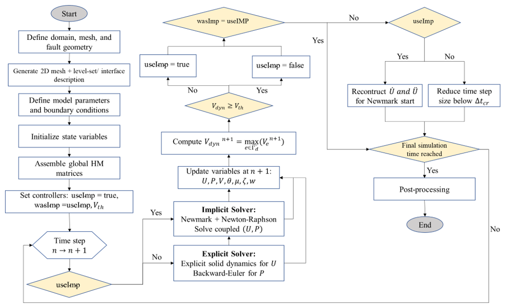
Figure 3 Schematic overview of the adaptive hybrid solution strategy. The model alternates between implicit and explicit solvers based on the fault slip-rate criterion V_dyn≥V_th, allowing stable treatment of quasi-static deformation and efficient resolution of dynamic rupture.

The main limitation of this formulation is that the hydraulic aperture is described by a local stress-dependent closure law. Thus, it does not explicitly resolve aperture heterogeneity, roughness-induced channeling, gouge migration, damage, chemical effects, or shear-induced permeability enhancement beyond the computed normal opening. Moreover, the cubic law assumes laminar flow between locally parallel plates, so the resulting permeability should be interpreted as an effective transmissivity rather than a fully resolved fault-pore structure. Despite these simplifications, the formulation consistently incorporates stress-dependent fault transmissivity while preventing nonphysical hydraulic closure under compressive contact.

3 Verification and model setup

The fully implicit hydromechanical formulation employed in this study has been previously verified and validated in detail in Sabah et al. (2026). That work included comprehensive verification against analytical solutions for saturated porous media (Wang, 2000), established numerical benchmarks for fractured porous systems (Damirchi et al., 2022), and the SEAS BP3-QD benchmark for assessing the rate-and-state friction implementation and the nucleation-stage slip evolution (Erickson et al., 2020). In the present study, the fully implicit formulation is adopted with modifications to the enforcement of contact constraints and is used as the reference solver. Building on this verified framework, the proposed hybrid solution strategy is introduced and systematically compared with the fully implicit reference solution in terms of fault response and numerical performance. To further assess the explicit elastodynamic component of the proposed hybrid framework, we also used the TPV205-2D dynamic rupture benchmark from the SCEC/USGS Earthquake Code Verification Exercise (Harris et al., 2009). It should be noted that TPV205-2D is based on a slip-weakening friction law rather than a rate-and-state friction law. Therefore, this benchmark is used specifically to verify the elastodynamic rupture component of the solver, rather than the rate-and-state friction implementation. For completeness, the verification results for both the fully implicit and explicit components of the framework are provided in the Supplement.

The computational domain is a square region measuring 400 m × 400 m, representing a horizontal cross-section of a fractured reservoir subjected to anisotropic in-situ stresses. As illustrated in Fig. 4, the pre-existing fault is represented in the XFEM discretization as a lower-dimensional, 1D line segment embedded in the 2D porous domain. Its end points are located at (100, 101 m) to (300, 301 m), giving a total fault length of about 282.8 m. The fault is orientated at 45° counterclockwise from the horizontal x axis. A fluid injection well is positioned near the fault center at (188, 212 m) to promote fault activation through pore-pressure diffusion and poroelastic stress redistribution.

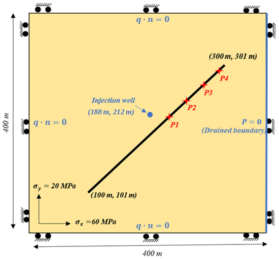
Figure 4 Schematic of a single-phase fluid injection scenario in a homogeneous porous formation containing a fault. The injection well is located at coordinates (188, 212 m), and the fault spans from (100, 101 m) to (300, 301 m). Four observation points along upper part of fault (denoted P1–P4) are used to monitor fault response. The reservoir is subjected to anisotropic in-situ compressive stresses of $\left|{\mathit{\sigma }}_x\right|=\mathrm{60}$ MPa and $\left|{\mathit{\sigma }}_y\right|=\mathrm{20}$ MPa, applied as initial stress conditions throughout the domain rather than as boundary tractions. All external boundaries are mechanically constrained by roller boundary conditions, allowing tangential displacement while preventing normal motion. The pore-pressure boundary condition is set to P=0 MPa (drained condition) along the right boundary, while the remaining boundaries are hydraulically impermeable.

All boundaries are mechanically constrained: the left and right boundaries are fixed in the x-direction, while displacements along the bottom and top boundaries are constrained in the y-direction. Uniform compressive in-situ stresses are applied within the domain, with ${\mathit{\sigma }}_x=-\mathrm{60}$ MPa and ${\mathit{\sigma }}_y=-\mathrm{20}$ MPa, where the negative sign denotes compression. Together with an initial friction coefficient of f₀=0.6, this stress state places the fault close to critical failure. The pore pressure boundary condition is set to P=0 MPa (drained condition) along the right edge, while the remaining boundaries are hydraulically impermeable. The initial pore pressure throughout the domain is set to P₀=0 MPa. The initial slip velocity along the fault is assumed to be equal to the reference slip velocity, V^*. During the simulations, the slip velocity is not allowed to decrease below this reference value, in order to avoid numerical singularities associated with the logarithmic dependence of the rate-and-state friction law at very small slip velocities. Figure 5 presents the initial fault conditions after mechanical equilibrium is reached. Specifically, Fig. 5a shows the distributions of shear stress, effective normal stress, and Coulomb ratio along the fault, while Fig. 5b shows the corresponding aperture distribution along the fault. Note that initial fault aperture before applying the mechanical loading w₀ is set to 0.001 m. After the model reaches mechanical equilibrium under the prescribed initial stress conditions, fluid injection is initiated at a constant rate of $\mathrm{5}\times {\mathrm{10}}^{-\mathrm{4}}$ m³ (s m)⁻¹ from the injection well at t=0 s and continues throughout the simulation period (36 h). This injection induces a progressive increase in pore pressure and associated poroelastic deformation in the vicinity of the fault. The entire domain is discretized using 40 000 bilinear quadrilateral elements (200 × 200 mesh). Rock, fault, and fluid properties are summarized in Table 1.

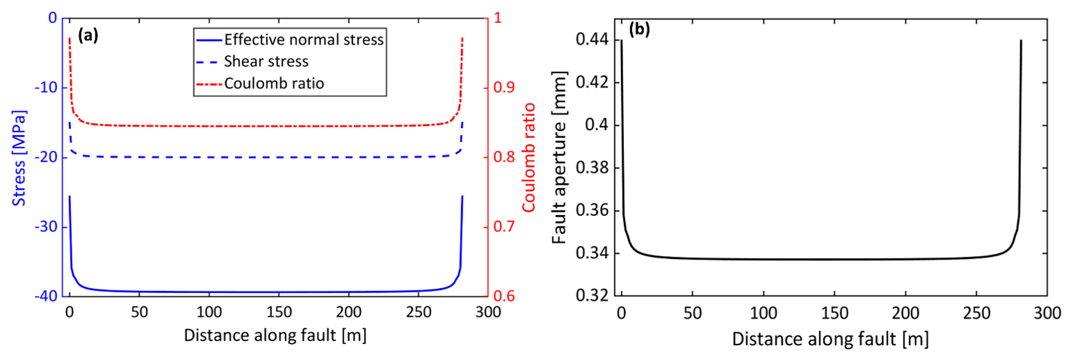
Figure 5 Initial fault conditions used in the simulations after reaching mechanical equilibrium: (a) distributions of effective normal stress, shear stress, and Coulomb ratio along the fault; and (b) corresponding initial fault aperture distribution. These equilibrated values are used as the starting state for the subsequent dynamic simulations.

The seismic moment and moment magnitude are calculated from the accumulated slip during individual seismic events. A seismic event is identified when the slip velocity of at least one fault element exceeds 0.1 m s⁻¹. Since the model is two-dimensional, an out-of-plane fault width of 1 m is assumed. The incremental seismic moment is calculated as

$$\begin{array}{}\text{(64)}& \mathrm{\Delta }{M}_{\mathrm{0},n}=G\sum _{e=\mathrm{1}}^{N_{\mathrm{f}}}{L}_e\mathrm{\Delta }{s}_{e,n}\end{array}$$

where G is the shear modulus, L_e is the length of fault element e, and Δs_e,n is its incremental slip at time step n. The cumulative seismic moment is evaluated separately for each event as

$$\begin{array}{}\text{(65)}& M_{\mathrm{0}}\left(t_n\right)=\sum _{j=n_{\mathrm{s}}}^n\mathrm{\Delta }{M}_{\mathrm{0},j}\end{array}$$

where n_s denotes the starting time-step index of the seismic event. The corresponding moment magnitude is calculated as

$$\begin{array}{}\text{(66)}& M_{\mathrm{w}}={\displaystyle \frac{\mathrm{2}}{\mathrm{3}}}\left({\log }_{\mathrm{10}}{M}_{\mathrm{0}}-\mathrm{9.05}\right)\end{array}$$

where M₀ is expressed in N m. Both seismic moment and moment magnitude are reported only during active seismic events. The average accumulated fault slip is independently calculated as

$$\begin{array}{}\text{(67)}& \stackrel{\mathrm{‾}}{s}\left(t_n\right)={\displaystyle \frac{{\sum }_{e=\mathrm{1}}^{N_{\mathrm{f}}}{L}_e{s}_{e,n}}{{\sum }_{e=\mathrm{1}}^{N_{\mathrm{f}}}{L}_e}}\end{array}$$

Unlike seismic moment, average slip is evaluated throughout the simulation and includes both seismic and aseismic contributions.

4 Results and discussion

4.1 Fully implicit solution

In this section, adaptive time stepping within the implicit solution framework is examined using three different minimum time-step sizes: 10⁻³, 10⁻⁴, and 10⁻⁵ s. An additional simulation with a minimum time-step size of 10⁻⁶ s is included in the temporal-convergence assessment presented in Fig. 7. The minimum time step represents the lower bound below which the adaptive algorithm is not allowed to further reduce the time increment. This analysis is motivated by the fact that, although the constant-average-acceleration Newmark scheme is unconditionally stable for linear structural-dynamics problems with the selected integration parameters, this property does not guarantee sufficient temporal accuracy for the complete nonlinear coupled fault system. In particular, during rupture nucleation and dynamic propagation, rapid variations in slip velocity, stress redistribution, and seismic response require adequate temporal resolution. Therefore, the effect of the prescribed minimum time-step size is investigated to assess its influence on the accuracy of the simulated dynamic rupture response. In all simulations, the maximum allowable time-step size is fixed at 3600 s.

Table 1 Material properties.

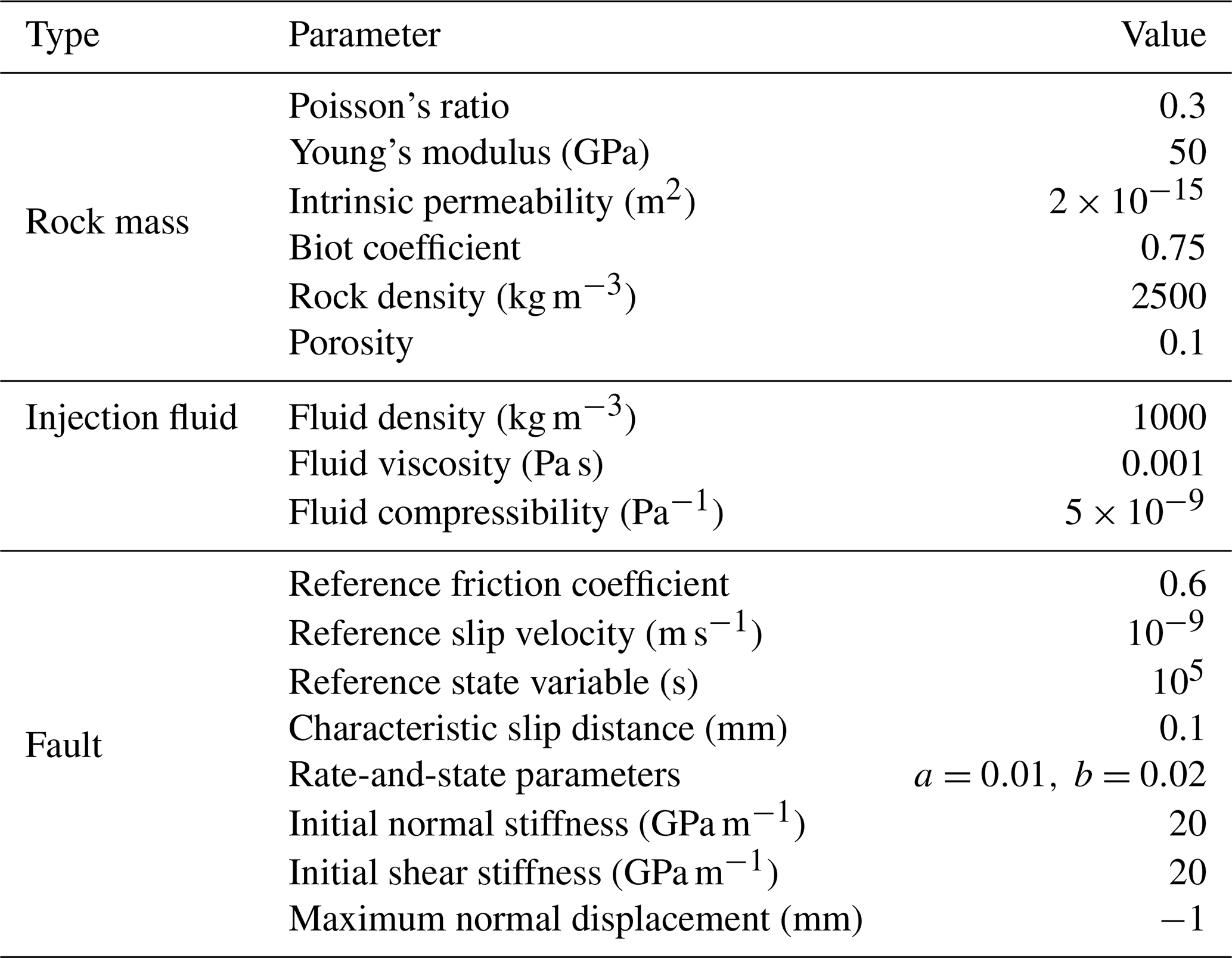
Figure 6 presents the simulation results for the three minimum time-step sizes. The right column corresponds to 10⁻³ s, the middle column to 10⁻⁴ s, and the left column to 10⁻⁵ s. The results indicate that a minimum time step of 10⁻³ s provides insufficient temporal resolution during the dynamic rupture phase. In contrast, reducing the minimum time step to 10⁻⁴ and 10⁻⁵ s leads to increased slip accumulation, higher peak slip rates, and earlier termination of the seismic phase. Despite these differences, the upper and lower bounds of the friction coefficient and shear stress remain largely unchanged across the three cases. It should be noted that the time axes in Fig. 6 are shifted independently according to the onset of dynamic rupture in each simulation. Consequently, these comparisons illustrate differences in the subsequent rupture evolution but do not directly quantify differences in the absolute onset time following fluid injection.

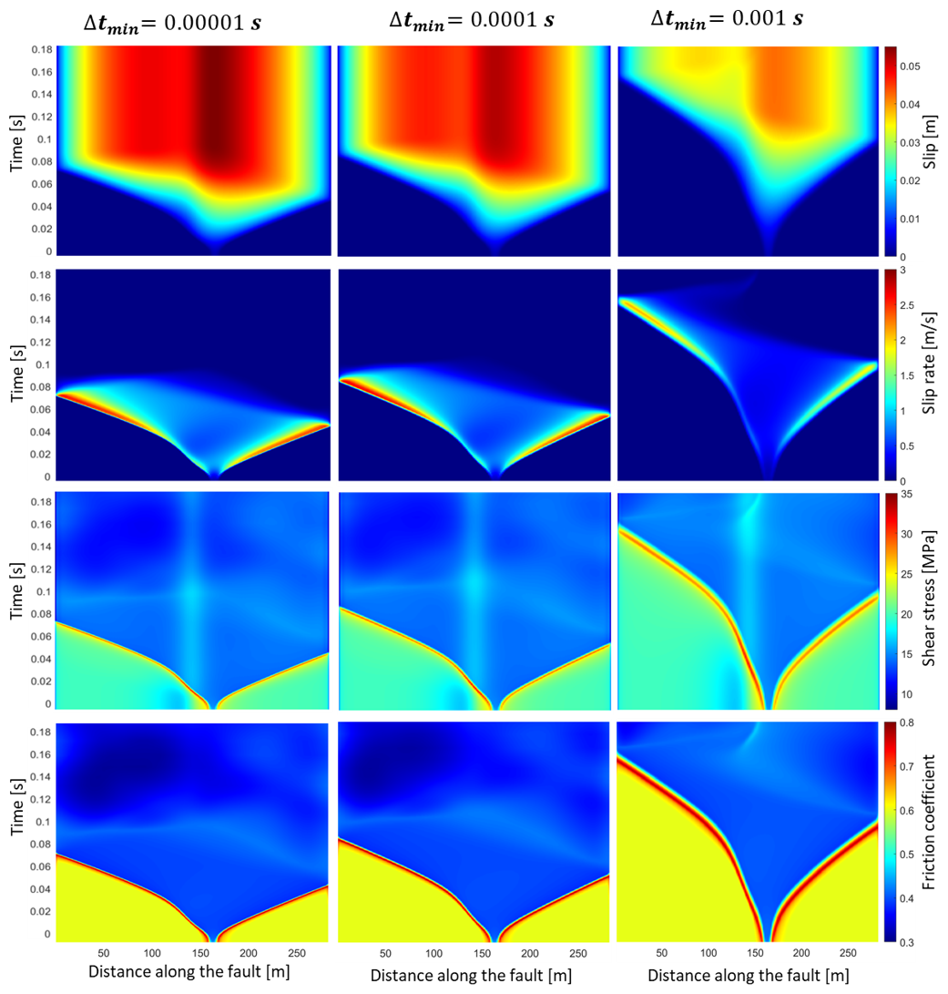
Figure 6 Space–time evolution of fault slip, slip rate, shear stress, and friction coefficient for three minimum time-step sizes: $\mathrm{\Delta }{t}_{\min }={\mathrm{10}}^{-\mathrm{5}}$ s (left), $\mathrm{\Delta }{t}_{\min }={\mathrm{10}}^{-\mathrm{4}}$ s (middle), and $\mathrm{\Delta }{t}_{\min }={\mathrm{10}}^{-\mathrm{3}}$ s (right). For each simulation, the time axis is shifted independently such that t=0 corresponds to the instant when the maximum slip velocity on the fault first exceeds 0.1 m s⁻¹. Therefore, the shifted time origin is used only to align the onset of dynamic rupture for comparison; the field variables at t=0 are not imposed to be identical and may differ due to differences in the preceding quasi-static/pre-dynamic evolution. Accordingly, the figure compares the dynamic response relative to the individual rupture-onset times rather than the absolute timing of rupture following fluid injection. The results highlight the influence of temporal resolution on rupture nucleation and the subsequent dynamic fault response.

Figure 7 compares the influence of different minimum time-step sizes on the simulated rupture dynamics in terms of average slip, seismic moment, moment magnitude, and rupture speed normalized by the shear wave velocity. Increasing the minimum time-step size generally leads to lower average slip, smaller seismic moments, and reduced rupture speeds (Fig. 7a, c, d). These discrepancies are particularly pronounced for a minimum time step of 10⁻³ s, indicating insufficient temporal resolution of the dynamic rupture process. In contrast, the differences in moment magnitude are relatively small due to its logarithmic dependence on seismic moment (Fig. 7b). The results obtained with minimum time steps of 10⁻⁵ and 10⁻⁶ s are nearly identical across all four quantities, indicating that the numerical solution has effectively converged with respect to temporal discretization for the investigated observables on the adopted spatial mesh. Therefore, a minimum time step of 10⁻⁵ s is considered an appropriate choice, providing a reasonable balance between numerical accuracy and computational efficiency.

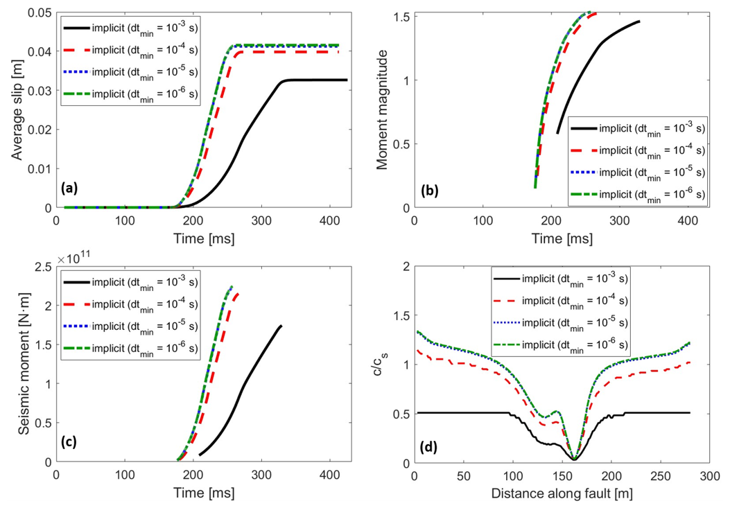
Figure 7 Influence of the minimum time-step size on event evolution for fully implicit simulations. Shown are the temporal evolutions of average fault slip (a), moment magnitude (b), and seismic moment (c), together with the spatial distribution of rupture speed normalized by the shear-wave velocity (d), for $\mathrm{\Delta }{t}_{\min }={\mathrm{10}}^{-\mathrm{3}},{\mathrm{10}}^{-\mathrm{4}},{\mathrm{10}}^{-\mathrm{5}}$, and 10⁻⁶ s. In panels (a)–(c), time is measured relative to a reference time corresponding to 21.7757 h after the onset of fluid injection (t=0). The results highlight the sensitivity of rupture timing, event magnitude, and rupture propagation speed to temporal resolution, with nearly identical responses obtained for minimum time-step sizes of 10⁻⁵ and 10⁻⁶ s, indicating temporal convergence for the reported observables on the adopted spatial mesh.

For the fully implicit simulations analyzed above, the time-step size is controlled adaptively using Eq. (55), in which the evolution-based time-step estimate is determined by the characteristic slip distance and the current slip velocity (Lapusta and Liu, 2009; Lapusta et al., 2000). This adaptive procedure is essential for resolving pre-dynamic processes such as nucleation, accelerating slip, and localization, and helps prevent important transient fault responses from being missed or delayed before the onset of fully dynamic rupture. However, because Eq. (55) imposes a prescribed lower bound on the time-step size, the adaptive algorithm cannot reduce the time increment below Δt_min, even when the slip-rate-based evolution criterion would require a smaller value. Consequently, the prescribed minimum time step directly influences the temporal resolution achievable during rapid fault acceleration and dynamic rupture. Once fully dynamic rupture develops, however, accurate resolution of rupture propagation and the associated wave field requires further reduction of the time-step size. The results demonstrate that, even within a fully implicit framework, the minimum time-step size needed to adequately resolve the dynamic rupture phase can be considerably smaller than wave-speed-based critical time-step estimate for the central-difference integration scheme (Eq. 61), which is approximately $\mathrm{2.3}\times {\mathrm{10}}^{-\mathrm{4}}$ s in the present case. It should be emphasized that this value represents an estimated stability limit based on the characteristic element size and elastic properties, rather than a rigorous stability bound for the complete XFEM system. In particular, the consistent mass matrix, Rayleigh damping, contact penalty stiffness, and enrichment functions may influence the highest frequencies of the spatially discretized system. Nevertheless, this estimate provides a useful reference for comparing stability-related and accuracy-related time-step requirements.

In addition, Lapusta and Liu (2009) proposed a minimum time-step estimate for achieving sufficient resolution of dynamic rupture propagation in elastodynamic simulations:

$$\begin{array}{}\text{(68)}& \mathrm{\Delta }{t}_{\mathrm{res}}=\mathit{\eta }\cdot \underset{e}{min}\left({\displaystyle \frac{l^{\mathrm{e}}}{c_{\mathrm{s}}}}\right)\end{array}$$

where η is constant, taken here as $\mathrm{1}/\mathrm{3}$ following Day et al. (2005), and c_s represents the shear wave speed. Using the material properties and mesh size adopted in the present simulations, this estimate gives $\mathrm{\Delta }{t}_{\mathrm{res}}=\mathrm{2.4}\times {\mathrm{10}}^{-\mathrm{4}}$ s. However, this estimate is substantially larger than the minimum time-step size required to obtain a temporally converged dynamic rupture response for the investigated quantities in the fully implicit simulations. This discrepancy highlights the distinction between numerical stability and temporal accuracy: although the fully implicit scheme is not subject to the same CFL stability restriction as the explicit scheme, accurately resolving dynamic rupture propagation and the associated seismic wave field still requires sufficiently small time steps, potentially well below the explicit CFL limit. Moreover, the characteristic wave-propagation resolution estimate in Eq. (68) does not explicitly account for the time scales associated with rapid frictional weakening, nonlinear slip acceleration, or changes in fault contact conditions. Consequently, satisfying such a wave-propagation-based estimate does not necessarily ensure that all aspects of the nonlinear rupture process are adequately resolved. The required time-step size must therefore be established through a convergence analysis of the relevant fault and seismic-response quantities.

Achieving this level of temporal resolution, however, comes at the expense of increased computational cost. Specifically, the CPU time increases from approximately 4.5 h for $\mathrm{\Delta }{t}_{\min }={\mathrm{10}}^{-\mathrm{3}}$ s to 10.9 h for $\mathrm{\Delta }{t}_{\min }={\mathrm{10}}^{-\mathrm{4}}$ s, and 26.4 h for $\mathrm{\Delta }{t}_{\min }={\mathrm{10}}^{-\mathrm{5}}$ s. A detailed assessment of the computational cost associated with different minimum time-step sizes, both with and without the inclusion of the slip tangent operator in the Jacobian assembly, is provided in Appendix A.

4.2 Hybrid solution approach

In the proposed solution strategy, the implicit solver efficiently resolves the quasi-static loading and nucleation phases, while a central-difference-based mechanical integration scheme is employed during dynamic fault slip and rupture propagation to reduce computational cost. The transition between the two integration schemes is controlled by the maximum slip velocity attained on any fault element. As described in Sect. 2.5.2, the dynamic mechanical formulation employs a consistent mass matrix and a non-diagonal damping matrix, including Rayleigh damping and absorbing-boundary contributions. Consequently, the acceleration update requires the solution of a global linear system rather than independent nodal operations. Nevertheless, this formulation avoids the global nonlinear Newton–Raphson iterations required by the fully implicit approach. The pore-pressure field remains implicitly integrated using the backward-Euler scheme, resulting in a sequentially coupled hydromechanical solution procedure during the dynamic phase. An important practical question is therefore the choice of an optimal slip-velocity threshold that minimizes the total computational cost while maintaining an acceptable level of agreement with the fully implicit reference solution, particularly during transient rupture propagation.

To assess the computational efficiency of the proposed hybrid time-integration strategy, we report the total CPU time required to complete each simulation and compare it with the corresponding fully implicit solution. For both the fully implicit and hybrid solution approaches, a minimum time-step size of $\mathrm{\Delta }{t}_{\min }={\mathrm{10}}^{-\mathrm{5}}$ s is prescribed. In the fully implicit approach, the time-step size is controlled adaptively throughout the entire simulation, with the prescribed minimum time step defining the lower bound of the adaptive algorithm. In the hybrid approach, the implicit phase employs the same adaptive time-stepping strategy, whereas the central-difference-based mechanical integration employs a fixed time step of 10⁻⁵ s during the dynamic phase, while the pore-pressure field is updated implicitly. This time-step size is substantially smaller than the wave-speed-based critical time-step estimate of $\mathrm{\Delta }{t}_{\mathrm{cr}}=\mathrm{2.3}\times {\mathrm{10}}^{-\mathrm{4}}$ s. As discussed in Sect. 4.1, the fully implicit computational time corresponding to $\mathrm{\Delta }{t}_{\min }={\mathrm{10}}^{-\mathrm{5}}$ s is approximately 26.4 h. Therefore, this value is adopted as the reference computational cost for evaluating the efficiency of the hybrid strategy.

Figure 8 illustrates the computational performance of the hybrid solution strategy for different switching slip-velocity thresholds, V_th. The results indicate that the hybrid approach substantially reduces the computational cost relative to the fully implicit simulation, with CPU-time reductions ranging from approximately 46 % to 62 %, depending on the selected threshold. As the threshold increases from $\mathrm{5}\times {\mathrm{10}}^{-\mathrm{4}}$ to 0.01 m s⁻¹, the hybrid CPU time decreases from approximately 14.29 to 10.00 h, corresponding to an increase in computational savings from 45.87 % to 62.12 %. The greatest computational efficiency is achieved at V_th=0.01 m s⁻¹, for which the hybrid simulation requires approximately 10  h, compared with 26.4 h for the fully implicit approach. This corresponds to a reduction of approximately 16.4 h in computational time. It should be emphasized that this reduction is obtained despite the use of consistent, non-diagonal mass and damping matrices during the central-difference-based mechanical integration. Therefore, the observed computational advantage does not arise from a strictly matrix-inversion-free explicit update, but from avoiding nonlinear global iterations during the dynamic phase.

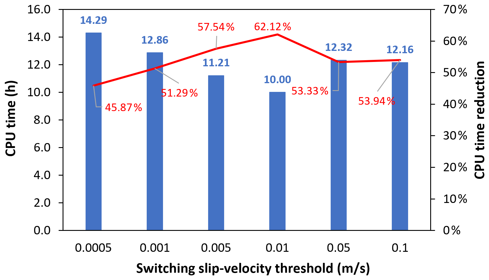
Figure 8 Computational performance of the hybrid solution strategy as a function of the slip-velocity threshold used to switch between implicit and central-difference-based mechanical integration. The minimum time-step size of the implicit solver and the fixed dynamic mechanical time step are both set to $\mathrm{\Delta }{t}_{\min }={\mathrm{10}}^{-\mathrm{5}}$ s. Shown are the total CPU time (blue bars) and the corresponding CPU-time reduction relative to fully implicit reference time of 26.4 h (red line). The maximum computational saving of 62.12 % occurs at a switching threshold of 0.01 m s⁻¹.

Further increasing the switching threshold beyond 0.01 m s⁻¹ reduces the computational advantage of the hybrid approach. Specifically, at V_th=0.05 and 0.1 m s⁻¹, the hybrid CPU times are approximately 12.32 and 12.16 h, respectively, corresponding to CPU-time reductions of 53.33 % and 53.94 %. This behavior suggests that excessively low switching thresholds may activate the central-difference-based mechanical solver prematurely, increasing the computational effort associated with the large number of small time steps and the corresponding global linear solves. Conversely, higher thresholds may prolong the computationally more demanding implicit phase, during which nonlinear global iterations are required. Consequently, an intermediate switching threshold of V_th=0.01 m s⁻¹ provides the most favorable balance between the implicit and dynamic mechanical integration contributions among the investigated values. Nevertheless, the identified threshold should be regarded as optimal only for the numerical configuration considered here, since the relative computational costs of the two integration schemes may depend on spatial discretization, constitutive parameters, damping properties, and the resulting fault slip-rate evolution. A more detailed comparison of the hybrid solution approach, with and without inclusion of the slip tangent operator during the implicit phase, together with its comparison against the fully implicit approach in terms of computational cost, is provided in Appendix B. It should be noted that the simulations presented in Appendix B employ a larger minimum time-step size of 10⁻⁴ s and therefore represent a separate computational-performance assessment.

Figure 9 compares the temporal evolution of the fault response at four observation points along the fault (P1–P4) obtained using the fully implicit and hybrid solution strategies. In the simulations using the hybrid approach, the transition from implicit to central-difference-based mechanical integration is triggered when the maximum slip velocity across the fault exceeds 0.01 m s⁻¹. This threshold determines the transition between numerical integration schemes and should be distinguished from the slip-velocity criterion of 0.1 m s⁻¹ used to identify the onset of a seismic event in the event-normalized analyses. The slip-rate histories (Fig. 9a) demonstrate that both approaches capture the onset, propagation, and overall sequence of dynamic rupture across the observation points. However, noticeable differences are observed in the timing and magnitude of peak slip rates. The hybrid approach generally predicts slightly delayed slip-rate peaks, particularly at P2–P4, and lower peak slip velocities compared with the fully implicit solution. These differences become more pronounced as the dynamic rupture accelerates toward the fault tips, while the overall rupture sequence and relative ordering of slip-rate peaks remain consistent. Since the time axes are referenced to a common time corresponding to 21.7757 h after the onset of fluid injection, these differences represent actual shifts in the simulated rupture evolution rather than artifacts introduced by independently aligning the rupture-onset times. The corresponding shear stress evolution (Fig. 9b) exhibits similar stress accumulation prior to instability, followed by a rapid stress drop during rupture. Although the hybrid solution shows slight temporal shifts in the stress peaks and subsequent stress drops, both approaches predict comparable post-rupture stress levels, with relatively small differences in the subsequent stress evolution.

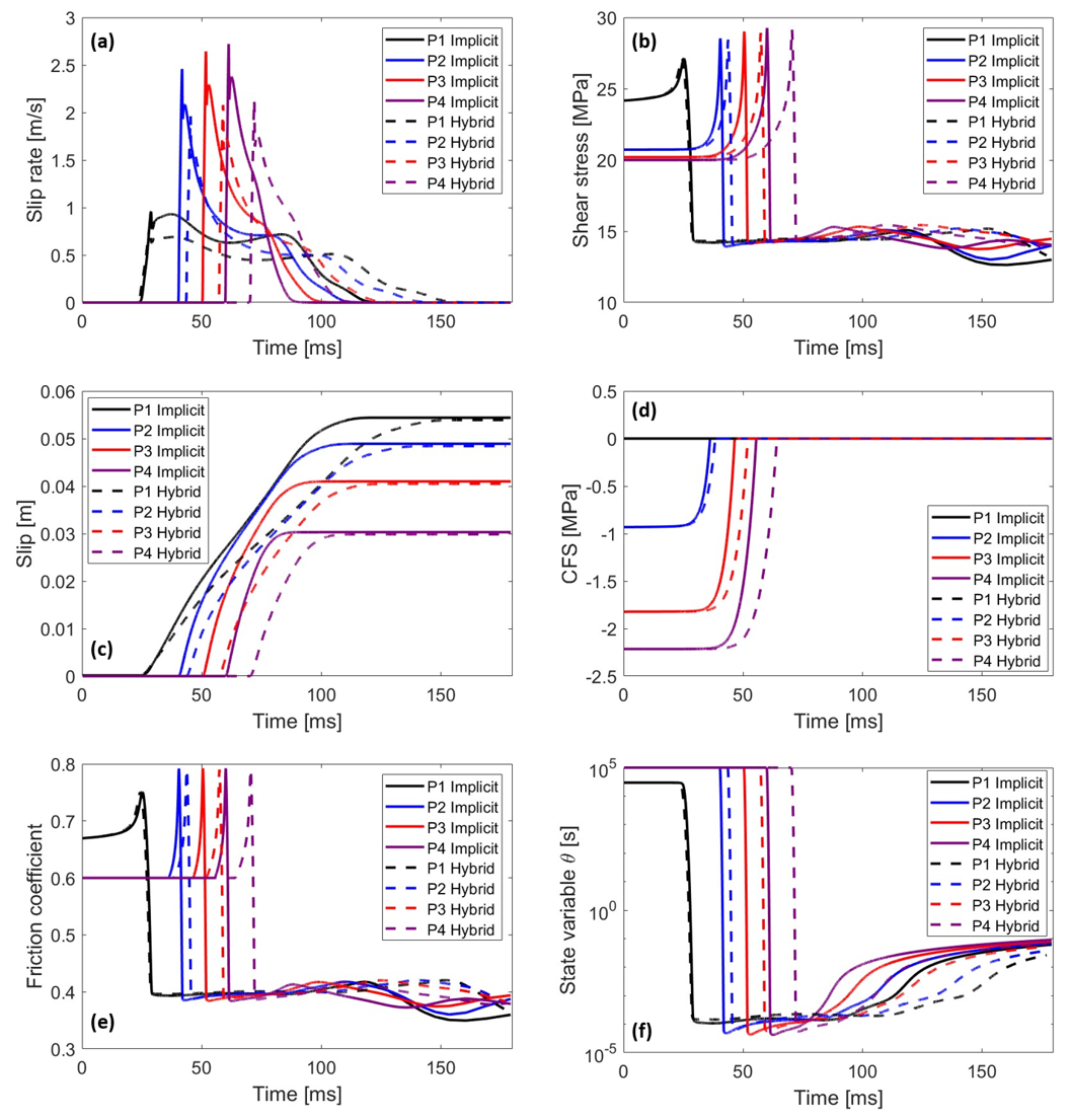
Figure 9 Comparison of fault response at four observation points along the fault (P1–P4) obtained using the fully implicit and hybrid solution strategies. Shown are the time histories of slip rate (a), shear stress (b), accumulated plastic slip (c), Coulomb failure stress (CFS) (d), friction coefficient (e), and state variable (f). Solid and dashed lines represent the fully implicit and hybrid solutions, respectively. In the hybrid approach, the transition from implicit to central-difference-based mechanical integration is triggered when the maximum slip velocity across all fault elements exceeds the prescribed threshold of 0.01 m s⁻¹. In all panels, time is measured relative to a common reference time corresponding to 21.7757 h after the onset of fluid injection (t=0). The common time reference enables direct comparison of differences in rupture timing and the evolution of fault variables between the two approaches.

The accumulated plastic slip histories (Fig. 9c) show close agreement between the two approaches in terms of final slip magnitudes at all observation points, despite differences in the timing and rate of slip accumulation. In particular, the hybrid solution exhibits a delayed accumulation of slip at several observation points, while converging toward nearly identical final slip values. This indicates that the differences in transient slip-rate histories have a limited influence on the overall accumulated slip. However, agreement in final accumulated slip should not be interpreted as demonstrating equivalent resolution of the transient rupture process, since the temporal evolution of slip and the associated peak slip velocities differ between the two schemes. Similarly, the evolution of Coulomb failure stress (CFS) (Fig. 9d) reveals comparable instability behavior, characterized by a rapid increase in CFS toward zero as rupture propagates along the fault. The hybrid solution reproduces this behavior with a slight delay at some observation points, consistent with the differences observed in the slip-rate and shear stress histories.

The friction coefficient evolution (Fig. 9e) exhibits a rapid change associated with the onset of dynamic instability, followed by pronounced frictional weakening during fault slip and relatively small fluctuations in the post-rupture phase. Both approaches capture the overall weakening behavior and predict comparable residual friction coefficients, although differences in the timing of the rapid weakening and subsequent evolution are evident. Finally, the state variable evolution (Fig. 9f) shows a sharp reduction during dynamic rupture, followed by a gradual increase during the post-seismic phase. The hybrid approach reproduces the characteristic evolution of the state variable, including its rapid decrease during instability and subsequent recovery, although the timing and rate of these changes differ slightly from those predicted by the fully implicit solution. These differences indicate that the integration strategy influences the temporal evolution of the frictional response, even when the final frictional state is similar. Overall, Fig. 9 demonstrates that the hybrid solution approach, using a switching slip-velocity threshold of 0.01 m s⁻¹, successfully reproduces the principal features of the fault response predicted by the fully implicit formulation, including rupture propagation, stress redistribution, accumulated plastic slip, and frictional evolution. Although some discrepancies are observed in the transient response, particularly in peak slip velocities and rupture timing, the close agreement in final slip magnitudes and post-rupture stress and frictional states indicates that the proposed hybrid strategy provides a reasonable approximation of the fully implicit solution while substantially reducing the computational cost.

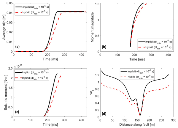
Figure 10 compares key event-scale seismicity metrics obtained using the fully implicit and hybrid solution strategies. The temporal evolution of average slip, moment magnitude, and seismic moment (Fig. 10a–c) demonstrates that both approaches capture the overall rupture evolution and predict comparable event magnitudes. However, the hybrid approach exhibits a delayed evolution of these quantities, with slower accumulation of average slip and seismic moment compared with the fully implicit solution. Despite these temporal differences, both approaches predict nearly identical final average slip values of approximately 0.041 m and comparable moment magnitudes of approximately 1.5, indicating that the overall event size is well reproduced by the hybrid formulation. These results suggest that the final event-scale quantities are relatively insensitive to the differences between the two integration schemes for the investigated configuration. However, the agreement in final average slip and moment magnitude does not imply identical temporal evolution of seismic moment release.

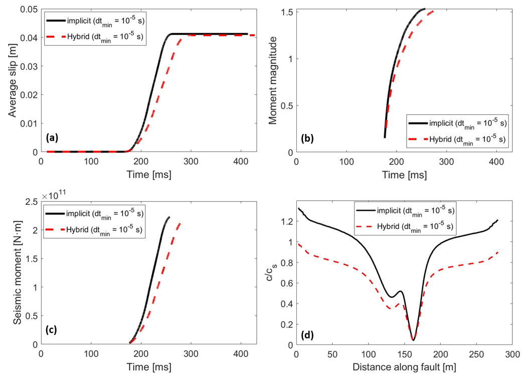
Figure 10 Comparison of event-scale seismicity metrics obtained using the fully implicit and hybrid solution strategies. Shown are the temporal evolutions of average slip (a), moment magnitude (b), and seismic moment (c), together with the spatial distribution of rupture speed normalized by the shear-wave velocity (d). In panels (a)–(c), time is measured relative to a common reference time corresponding to 21.7757 h after the onset of fluid injection (t=0). Both approaches reproduce comparable final average slip (approximately 0.041 m) and moment magnitude (approximately 1.5), although the hybrid solution exhibits a delayed evolution of these quantities. The fully implicit solution generally predicts higher rupture speeds, while both approaches capture a similar spatial distribution along the fault. The comparison indicates close agreement in the final event size but noticeable differences in rupture timing and propagation speed.

More pronounced discrepancies are observed in the spatial distribution of normalized rupture speed (Fig. 10d), where the fully implicit solution consistently predicts higher rupture velocities than the hybrid approach across most of the fault. Nevertheless, both methods exhibit a similar spatial pattern, characterized by a pronounced reduction in rupture speed near the central portion of the fault and increasing velocities toward the fault tips. The lower rupture speeds predicted by the hybrid approach are consistent with the delayed slip-rate peaks observed at the fault observation points in Fig. 9. This indicates that, although the hybrid strategy captures the overall spatial pattern of rupture propagation, quantitative differences remain in the predicted rupture-front dynamics. These results demonstrate that the hybrid solution strategy reasonably reproduces the principal characteristics of rupture evolution and seismic moment release obtained with the fully implicit formulation, although differences remain in rupture timing and propagation speed. These discrepancies highlight an important distinction between agreement in final seismic-source parameters and agreement in transient rupture dynamics. In particular, the computational advantage of the hybrid approach should be considered alongside its ability to resolve rupture-front propagation and the temporal evolution of seismic moment release. The results therefore illustrate a trade-off between computational efficiency and agreement with the fully implicit reference in transient dynamic quantities, while the hybrid approach provides substantial reductions in computational cost.

Figure 11 compares the synthetic particle-motion histories at the location of the injection well obtained using the fully implicit and hybrid solution approaches. The acceleration time histories (Fig. 11a–b) show that both approaches capture the overall characteristics of the dynamic response, although noticeable differences are observed in the peak amplitudes and subsequent oscillations. In particular, the hybrid approach predicts higher peak accelerations in both the X and Y directions compared with the fully implicit solution. The velocity histories (Fig. 11c–d), in contrast, indicate that the fully implicit approach produces higher peak particle velocities, while the hybrid solution exhibits lower amplitudes and slight temporal shifts in the subsequent oscillations. Despite these differences, both approaches reproduce similar oscillatory patterns, with the particle velocities gradually decreasing toward zero following the main dynamic event. The differences in peak acceleration and velocity indicate that the two integration schemes do not reproduce identical transient particle-motion amplitudes, even though the overall oscillatory response is similar.

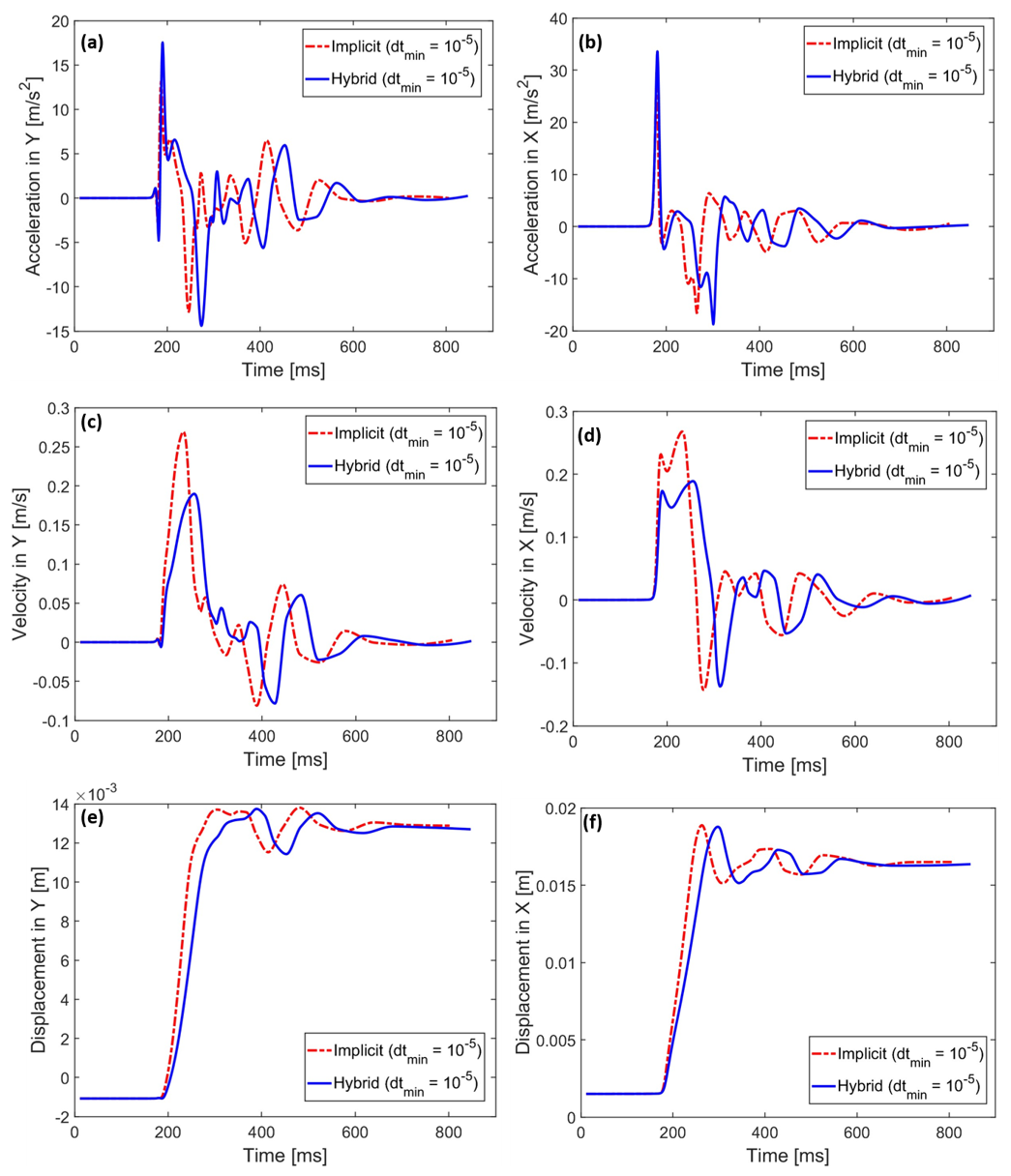
Figure 11 Comparison of acceleration, velocity, and displacement time histories at the location of the injection well obtained using the fully implicit and hybrid solution approaches. Shown are the acceleration components in the Y (a) and X (b) directions, velocity components in the Y (c) and X (d) directions, and displacement components in the Y (e) and X (f) directions. In all panels, time is measured relative to a reference time corresponding to 21.7757 h after the onset of fluid injection (t=0). The hybrid approach predicts higher peak accelerations, whereas the fully implicit solution yields higher peak velocities. Despite slight differences in the timing and amplitude of the transient response, both approaches converge to nearly identical final displacements in both directions. The comparison highlights the close agreement in final deformation while demonstrating that the transient acceleration and velocity responses remain sensitive to the adopted time-integration strategy.

The displacement histories (Fig. 11e–f) exhibit close agreement between the two approaches, although the hybrid solution shows a slightly delayed displacement accumulation during the initial stages of dynamic motion. Nevertheless, both approaches converge to nearly identical final displacement values in both directions, indicating that the differences in transient acceleration and velocity responses have a limited influence on the final deformation. This agreement is consistent with the similarity in final fault slip and seismic moment reported in Figs. 9 and 10. However, the close agreement in final displacement does not necessarily imply equivalent resolution of the transient seismic wave field, for which the acceleration and velocity amplitudes remain important indicators.

Overall, these results demonstrate that the hybrid solution strategy successfully reproduces the principal characteristics of the dynamic particle-motion response and final displacement predicted by the fully implicit formulation, despite noticeable discrepancies in peak acceleration and velocity amplitudes. Thus, the hybrid formulation provides a close approximation of the final deformation response for the investigated problem, while differences remain in the transient particle-motion characteristics. These differences should be considered when evaluating the applicability of the proposed approach to problems requiring accurate prediction of dynamic ground-motion amplitudes or detailed seismic waveforms. Spatial distributions of acceleration, velocity, and displacement over the computational domain during the seismic event, obtained using both the fully implicit and hybrid solution approaches, are provided in Appendix C. These additional results provide a spatial comparison of the dynamic response at corresponding event-normalized stages, complementing the fixed-location time histories presented in Fig. 11.

5 Conclusion

This study introduced a hybrid time-integration strategy for simulating injection-induced fault reactivation within a fully coupled poroelastodynamic XFEM framework. The proposed approach directly addresses the fundamental challenge posed by the extreme separation of time scales inherent to fluid-driven seismicity, ranging from slow reservoir pressurization to rapid fault nucleation and dynamic rupture. Using a fully implicit poroelastodynamic formulation as a reference solution, we demonstrated that although the adopted constant-average-acceleration Newmark scheme is unconditionally stable for linear structural-dynamics problems with the selected integration parameters, this property does not guarantee sufficient temporal accuracy for the nonlinear coupled fault system. Insufficient temporal resolution leads to delayed instability, underestimated slip rates, and reduced seismic moments. The sensitivity analysis revealed that minimum time-step sizes of 10⁻⁵ and 10⁻⁶ s produce nearly identical results in terms of average slip, seismic moment, moment magnitude, and rupture propagation speed, indicating temporal convergence for these observables at 10⁻⁵ s on the adopted spatial mesh. Notably, this time-step size is substantially smaller than the wave-speed-based critical time-step estimate for central-difference integration $(\mathrm{\Delta }{t}_{\mathrm{cr}}=\mathrm{2.3}\times {\mathrm{10}}^{-\mathrm{4}}$ s). These findings highlight the distinction between numerical stability and temporal accuracy in fully implicit simulations of dynamic fault rupture, where sufficiently small time steps are required despite the absence of a conventional CFL stability restriction.

To improve computational efficiency while maintaining adequate temporal resolution, the proposed hybrid strategy advances the system implicitly during quasi-static loading and nucleation phases and automatically transitions to a central-difference-based mechanical integration scheme once a prescribed slip-velocity threshold is exceeded. During the dynamic phase, a fixed time-step size of 10⁻⁵ s is employed to resolve the rapid fault response, while the pore-pressure field continues to be advanced using backward-Euler integration. The numerical comparisons demonstrated that this solver-switching strategy reproduces the principal characteristics of fault slip, shear stress evolution, frictional weakening, Coulomb failure stress, and seismic moment release while substantially reducing computational cost. Depending on the selected slip-velocity threshold, the hybrid approach yielded CPU-time reductions of approximately 46 %–62 % relative to the fully implicit reference. The greatest computational saving was obtained at a switching threshold of 0.01 m s⁻¹, for which the hybrid simulation required approximately 10 h compared with 26.4 h for the fully implicit solution, corresponding to a CPU-time reduction of 62.12 %. This computational advantage is therefore achieved despite the need for global linear solves during the dynamic mechanical phase and is primarily associated with avoiding repeated nonlinear iterations.

Comparisons of fault-scale and event-scale responses showed that the hybrid formulation reproduces the overall rupture sequence, spatial propagation patterns, and final accumulated slip with close agreement to the fully implicit solution. However, noticeable discrepancies were observed in the transient dynamic response, particularly in the timing and magnitude of peak slip velocities and rupture propagation speeds. The hybrid approach generally predicts delayed and lower peak slip velocities, while the fully implicit solution yields higher rupture speeds across most of the fault. Despite these differences, both approaches predict nearly identical final average slip values of approximately 0.041 m and comparable moment magnitudes of approximately 1.5, indicating that the overall event size is well reproduced by the hybrid formulation. Furthermore, comparisons of synthetic particle-motion histories at the injection well revealed higher peak accelerations in the hybrid solution and higher peak particle velocities in the fully implicit solution. Nevertheless, both approaches converge to nearly identical final displacements in both directions, suggesting that the differences in transient wave characteristics have a limited influence on the final deformation. These results demonstrate that close agreement in final fault slip, seismic moment, and displacement does not necessarily imply equivalent resolution of transient rupture dynamics and seismic wave propagation. Therefore, although the hybrid formulation reproduces the principal event-scale characteristics of the fully implicit reference, differences in rupture timing, propagation speed, and particle-motion amplitudes should be considered when evaluating its accuracy for applications requiring detailed dynamic wave-field predictions.

An important practical outcome of this study is the demonstration that, within the hybrid solution framework, the slip tangent operator can be omitted during the implicit phase without eliminating the computational advantage of the proposed strategy, although its inclusion improves nonlinear convergence and reduces CPU time. This finding is particularly relevant for more complex frictional constitutive models and potentially larger-scale or three-dimensional simulations, where construction and evaluation of the consistent frictional tangent operator can become computationally demanding.

Overall, the proposed XFEM framework combined with the hybrid implicit–explicit time-integration strategy provides a computationally efficient numerical approach for simulating injection-induced reactivation of a prescribed pre-existing fault within the investigated two-dimensional configuration. The results demonstrate that using implicit integration during slowly evolving deformation and central-difference-based mechanical integration during rapid rupture can resolve multi-scale fault-slip processes while reducing computational cost for the present two-dimensional homogeneous benchmark problem. Although the hybrid approach introduces noticeable deviations in certain transient rupture characteristics, the close agreement in final slip, seismic moment release, and deformation indicates a favorable balance between computational efficiency and agreement with the fully implicit reference for the investigated configuration. Nevertheless, this agreement should not be interpreted as demonstrating identical transient dynamic accuracy, particularly in the prediction of rupture-propagation speeds and seismic wave amplitudes. The observed computational savings indicate the potential of the proposed hybrid strategy for larger-scale simulations, although systematic spatial-refinement and scalability assessments, together with investigations involving heterogeneous media, more complex fault geometries, and different frictional conditions, are required to establish its broader applicability and robustness.

6 Limitations and future work

The present study is limited to a moderate-size two-dimensional benchmark problem with a prescribed pre-existing fault in a homogeneous medium. Therefore, the reported CPU-time reduction should be interpreted as a relative efficiency improvement for the numerical setup considered here, rather than as a formal demonstration of scalability or operational readiness. A comprehensive scalability assessment would require simulations with progressively larger meshes and degrees of freedom, together with detailed reporting of assembly time, solver time, nonlinear iterations, time-step counts, memory use, preconditioner performance, and parallel efficiency. Such an analysis is beyond the scope of the present work.

Future work could focus on extending the framework toward larger and more realistic problems, including three-dimensional fault systems, heterogeneous poroelastic media, thermo-hydro-mechanical coupling, more complex frictional and permeability evolution laws, and fault-network interactions. Further developments should also include the formulation of a physics-based, non-dimensional switching criterion that can improve computational efficiency while remaining applicable across different geological conditions. In addition, systematic mesh-refinement and scaling studies, implementation of efficient parallel solvers and preconditioners, and validation against field-scale observations are needed. Such extensions are necessary before the proposed framework can be considered for operational induced-seismicity forecasting in subsurface energy applications.

Appendix A: Effect of slip tangent operator in fully implicit solution approach

From a computational perspective, we compared two prescribed minimum time-step sizes ($\mathrm{\Delta }{t}_{\min }={\mathrm{10}}^{-\mathrm{4}}$ s and $\mathrm{\Delta }{t}_{\min }={\mathrm{10}}^{-\mathrm{3}}$ s) in terms of total CPU time and the number of nonlinear iterations required for convergence. The comparison was performed both with and without the consistent slip tangent operator developed in Sect. 2.5.1 (Eq. 51). It should be noted that the time-step size directly influences the effective Jacobian matrix through the coefficients introduced by the Newmark and backward-Euler time discretizations, as well as through the time-step-dependent rate-and-state friction formulation. Consequently, changes in the time-step size modify the Jacobian coefficients and may affect the convergence characteristics of the nonlinear system. However, the primary objective of the present comparison is to evaluate the computational benefit of including the consistent local slip tangent contribution in the global Jacobian assembly. When this contribution is omitted, the resulting Jacobian provides an approximate linearization of the interface constitutive response, potentially increasing the number of Newton–Raphson iterations required for convergence, particularly during rapid fault acceleration and frictional weakening. It should also be emphasized that the minimum time-step sizes investigated in this appendix are larger than the value of 10⁻⁵ s identified in Sect. 4.1 as sufficient for temporal convergence of the selected rupture observables. Therefore, the present analysis focuses on computational performance and nonlinear convergence rather than establishing temporal accuracy.

For $\mathrm{\Delta }{t}_{\min }={\mathrm{10}}^{-\mathrm{4}}$ s, a balance between computational cost and temporal resolution is considered , the fully implicit scheme including the slip tangent operator required 10.95 h of CPU time. Omitting the operator increased the runtime to 15.25 h, corresponding to an approximately 39 % increase in CPU time, or equivalently a 28 % reduction when the slip tangent is included (Fig. A1a). This indicates that, for the smaller of the two investigated minimum time-step sizes, omitting the slip tangent operator increases the computational cost but does not prevent the nonlinear solver from reaching convergence. The additional computational effort arises from the increased number of Newton–Raphson iterations required when the sensitivity of the frictional traction to displacement changes is not fully represented in the Jacobian. This observation is relevant for more complex friction laws, for which deriving and implementing a consistent local tangent operator may be considerably more difficult. In contrast, when a larger minimum time-step size is prescribed ($\mathrm{\Delta }{t}_{\min }={\mathrm{10}}^{-\mathrm{3}}$ s), the computational benefit of including the slip tangent operator becomes considerably more pronounced. In this case, the fully implicit simulation requires approximately 4.52 h with the slip tangent operator and 14.54 h without it (Fig. A1b). Therefore, omitting the slip tangent increases the computational time by approximately 222 % relative to the simulation including the operator, whereas including the operator reduces the computational time by approximately 69 % relative to the simulation without it. This substantially larger performance difference is associated with the stronger nonlinear variations that may develop within the larger time increments, particularly during rapid slip acceleration and frictional weakening. Under these conditions, the approximate Jacobian requires considerably more Newton–Raphson iterations to satisfy the prescribed convergence tolerance. Thus, although the time-step size directly affects the effective Jacobian coefficients, the additional computational advantage of including the slip tangent operator arises primarily from a more accurate linearization of the nonlinear interface response, leading to improved convergence and reduced total solution time.

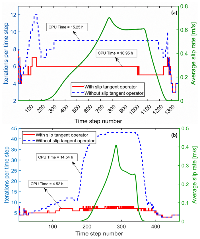
Figure A1 Solver performance with and without the slip tangent operator for two minimum time-step sizes. Shown are the Newton iterations per time step for $\mathrm{\Delta }{t}_{\min }={\mathrm{10}}^{-\mathrm{4}}$ s (a) and $\mathrm{\Delta }{t}_{\min }={\mathrm{10}}^{-\mathrm{3}}$ s (b), together with the average slip rate. Inclusion of the slip tangent operator reduces iteration counts and total CPU time, with the strongest efficiency gain observed for the larger time step.

Appendix B: Effect of slip tangent operator in hybrid solution approach

Figure B1 illustrates the computational efficiency of the hybrid solution strategy with and without including the slip tangent operator during the implicit phase, for a range of slip-velocity thresholds controlling the solver transition. A minimum time-step size of $\mathrm{\Delta }{t}_{\min }={\mathrm{10}}^{-\mathrm{4}}$ s is used for the implicit solver and also adopted as the explicit time step. Overall, for both approaches, the CPU time reaches its minimum at a switching velocity of 0.01 m s⁻¹ (Fig. B1a). Specifically, the CPU time decreases from 4.75 and 4.5 h at a switching velocity of $\mathrm{5}\times {\mathrm{10}}^{-\mathrm{4}}$ m s⁻¹ to 3.76 and 3.15 h at 0.01 m s⁻¹ for the cases without and with the slip tangent operator, respectively. Interestingly, in contrast to the fully implicit approach, omitting the slip tangent operator within the hybrid solution framework does not lead to a substantial increase in computational cost. For example, excluding the slip tangent operator results in a minimum increase of approximately 5.5 % and a maximum increase of approximately 31 % in CPU time, occurring at switching velocities of $\mathrm{5}\times {\mathrm{10}}^{-\mathrm{4}}$ and 0.1 m s⁻¹, respectively. The comparison with the fully implicit scheme (Fig. B1b) including the slip tangent operator is particularly significant. At a switching velocity of 0.01 m s⁻¹, the hybrid approach reduces the CPU time by 71.27 % and 65.65 % with and without the slip tangent operator, respectively. These results indicate that, within the hybrid framework, the slip tangent operator can be neglected without severely compromising computational efficiency. This is particularly advantageous when the evaluation of the corresponding Jacobian terms becomes complex or computationally demanding.

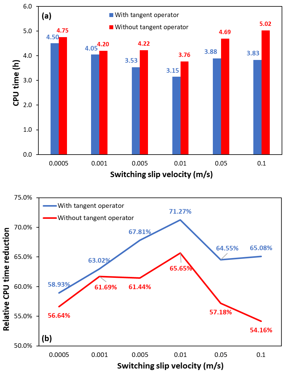
Figure B1 Computational performance of the hybrid solution strategy for different switching slip velocities, with and without inclusion of the slip tangent operator during the implicit phase. The minimum implicit time-step size is set to $\mathrm{\Delta }{t}_{\min }={\mathrm{10}}^{-\mathrm{4}}$ s, which is also used as the fixed explicit time step. (a) CPU time required by the hybrid solution-based simulations. For both formulations, the minimum CPU time is obtained at a switching slip velocity of 0.01 m s⁻¹. (b) Relative CPU time reduction of the hybrid strategy with respect to the fully implicit scheme including the slip tangent operator.

Appendix C: Acceleration, velocity, and displacement field during seismic events

Figures C1–C3 show the spatial distributions of acceleration, velocity, and displacement over the computational domain during the seismic events simulated using both the fully implicit and hybrid solution approaches. A minimum time-step size of $\mathrm{\Delta }{t}_{\min }={\mathrm{10}}^{-\mathrm{5}}$ s is used for the implicit solver and also adopted as the explicit time step. A seismic event is defined to begin when the slip velocity on any fault patch exceeds 0.1 m s⁻¹, and the time displayed above each snapshot is measured relative to this onset time. For each solution approach, the corresponding fields are presented at 25 %, 50 %, and 75 % of the event duration. This event-normalized comparison provides a more meaningful basis for evaluating the two approaches, because the hybrid solution exhibits a delay of a few milliseconds relative to the fully implicit solution. Therefore, comparing the two solutions at the same absolute time after injection would not be appropriate, particularly because the entire seismic event lasts only about 0.1 s. The results further support the findings presented in Fig. 11, showing that the hybrid solution approach reproduces the acceleration, velocity, and displacement distributions obtained with the fully implicit approach, as well as their spatial propagation around the fault during rupture. For the acceleration field (Fig. C1), the hybrid approach produces slightly higher values, whereas for the velocity field (Fig. C2), it gives slightly lower values, particularly near the rupture front. However, as discussed previously, these differences are not significant. For the displacement field (Fig. C3), both approaches yield almost identical spatial distributions.

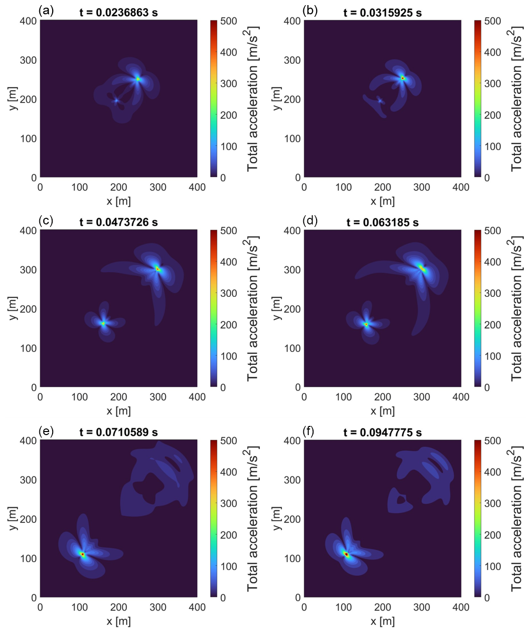
Figure C1 Spatial distribution of total acceleration during the seismic event obtained using the hybrid solution approach (left column: a, c, e) and the fully implicit solution approach (right column: b, d, f). A seismic event is defined to begin when the slip velocity on any fault patch exceeds 0.1 m s⁻¹, and the time displayed above each snapshot is measured relative to this onset time. For each solution approach, the acceleration field is shown at 25 %, 50 %, and 75 % of the corresponding event duration, enabling an event-normalized comparison between the two approaches despite the small time delay between them.

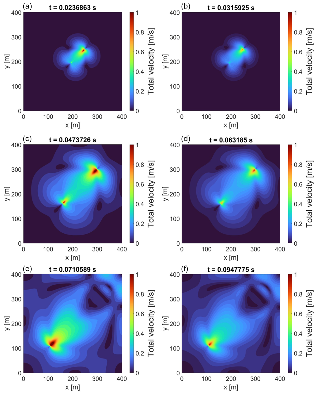
Figure C2 Spatial distribution of total velocity during the seismic event obtained using the hybrid solution approach (left column: a, c, e) and the fully implicit solution approach (right column: b, d, f). A seismic event is defined to begin when the slip velocity on any fault patch exceeds 0.1 m s⁻¹, and the time displayed above each snapshot is measured relative to this onset time. For each solution approach, the velocity field is shown at 25 %, 50 %, and 75 % of the corresponding event duration, enabling an event-normalized comparison between the two approaches despite the small time delay between them.

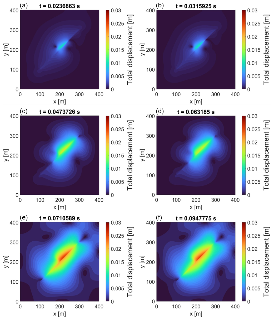
Figure C3 Spatial distribution of total displacement during the seismic event obtained using the hybrid solution approach (left column: a, c, e) and the fully implicit solution approach (right column: b, d, f). A seismic event is defined to begin when the slip velocity on any fault patch exceeds 0.1 m s⁻¹, and the time displayed above each snapshot is measured relative to this onset time. For each solution approach, the displacement field is shown at 25 %, 50 %, and 75 % of the corresponding event duration, enabling an event-normalized comparison between the two approaches despite the small time delay between them.