Slope-Constrained Orography (SCO v1.0) for explicit discrete-slope control in terrain preprocessing: a case study with WRF-ARW (v4.6.1)

Kilometre-scale Weather Research and Forecasting (WRF) simulations over terrain with steep slopes often require strong smoothing to prevent numerical instability, but conventional domain-wide filters alter terrain at every grid point, regardless of whether local slopes require reduction. Slope-Constrained Orography (SCO) is an offline terrain preprocessing method that prescribes a target slope angle θ and adjusts only those grid points whose eight-neighbour elevation differences exceed the implied bound, leaving the remaining terrain unchanged. By prescribing the slope constraint directly, SCO provides a geometrically interpretable primary user-facing parameter for terrain construction and stability testing. In a 1 km WRF case over the highly complex terrain of the southeastern Tibetan Plateau, the least-modified stable SCO member among those tested modifies 14 % of points with a mean elevation change of 8.2 m, compared with 100 % modification and 108.1 m for the corresponding WRF Preprocessing System (WPS) member. The successful SCO configuration produces lower near-surface wind and temperature errors in this case.

1 Introduction

Complex terrain exerts strong control on boundary-layer flow, thermally driven circulations, and orographic precipitation (Raderschall et al., 2008; Cannon et al., 2017; Díaz-Fernández et al., 2025), motivating the use of kilometre-scale grids to resolve ridge–valley structure. In terrain-following coordinate models such as the Weather Research and Forecasting model (WRF; Skamarock et al., 2019), the large elevation differences that arise on kilometre-scale grids over complex terrain amplify horizontal pressure-gradient errors and can trigger numerical instability within a few time steps (Mahrer, 1984; Klemp et al., 2003; Zängl et al., 2004). Terrain preprocessing is therefore necessary, but the smoothing required to prevent instability routinely modifies terrain well beyond the grid points that actually govern stability.

In the standard WRF Preprocessing System (WPS) workflow, geogrid applies a single pass of smth-desmth_special smoothing to the terrain field across the entire domain. Over steep terrain at kilometre-scale grid spacing, one pass is often insufficient, and users must increase the pass count, an integer parameter with no direct geometric correspondence to the resulting slope field. The maximum discrete slope that emerges depends on the raw terrain, the grid spacing, and the number of passes, and can only be diagnosed after the smoothing is complete. Because the filter updates every grid point at each iteration, terrain changes propagate far from the locations that control stability. Successive iterations yield diminishing reductions in peak slope, and stability can only be verified by completing a trial integration.

Modifying the vertical coordinate offers an alternative path to accommodating steep slopes (Park et al., 2019; Ma and Liu, 2017), but localised terrain adjustments have also been explored within conventional preprocessing. Sheridan et al. (2023) blended lightly and heavily smoothed terrain across steep-slope regions; Raluy-López et al. (2026) applied a local Gaussian filter only to grid points exceeding a slope threshold; and Le Bouëdec et al. (2025) posed terrain adjustment as a constrained optimisation problem with prescribed slope bounds. Slope-Constrained Orography (SCO) follows a similar motivation: it prescribes a target slope angle θ as the primary user-facing parameter and adjusts only those grid points whose eight-neighbour elevation differences exceed the implied bound, leaving the rest of the terrain unchanged.

This study introduces SCO v1.0 and evaluates it against standard WPS smoothing in 1 km Advanced Research WRF (WRF-ARW) v4.6.1 simulations over the highly complex terrain of the southeastern Tibetan Plateau. Three questions guide the evaluation: (1) can a prescribed-slope approach produce stable 48 h integrations with substantially less terrain modification than domain-wide smoothing, (2) how do the two methods differ in slope-field structure near the stability boundary, and (3) how do near-surface forecast errors compare between their successful configurations in this case?

2 Method and WRF implementation

2.1 Overview

SCO adjusts terrain elevation on a structured grid using working bounds on eight-neighbour elevation differences derived from a prescribed slope angle θ. Water bodies and lateral boundaries remain fixed throughout. The adjustment proceeds through weighted pairwise projection. Whenever the elevation difference across a neighbour pair exceeds a local bound, the solver redistributes the excess between the two endpoints in proportion to their mobility weights. The bounds include a conservative geometric scaling, explained in Sect. 2.2. Inner stopping conditions and a separate outer acceptance test determine when iteration ends (Sect. 2.3). The implementation assumes uniform grid spacing (Δx=Δy).

Because SCO operates on the standard geo_em files produced by geogrid, it integrates easily into the existing WPS pipeline between geogrid and metgrid with no modifications to the WRF source code. Here, geogrid interpolates static geographical data, including terrain, to the model grids, while metgrid interpolates meteorological fields horizontally to the same grids. The Python implementation reads and writes geo_em.d0X.nc directly and is used here for both offline diagnostics and terrain construction. Source code, documentation, and a worked example are archived on Zenodo (see Code and data availability).

2.2 Discrete slope metric and constraint derivation

The target angle θ is the user-prescribed slope parameter. Let h_i,j denote terrain height on a grid with spacing Δx. The local eight-neighbour discrete slope angle is

$$\begin{array}{}\text{(1)}& S_{i,j}=\underset{(m,n)\in {\mathcal{N}}_{\mathrm{8}}(i,j)}{max}\arctan \left({\displaystyle \frac{|h_{m,n}-h_{i,j}|}{d_{(i,j),(m,n)}}}\right),\end{array}$$

where d=Δx for cardinal neighbours and $d=\sqrt{\mathrm{2}}\mathrm{\Delta }x$ for diagonal neighbours. The eight neighbours comprise the four cardinal points $(i\pm \mathrm{1},j)$, $(i,j\pm \mathrm{1})$ and the four diagonal points $(i\pm \mathrm{1},j\pm \mathrm{1})$. Taking the maximum detects an exceedance in any sampled direction; averaging could conceal a single steep pair. The maximum over the active interior is denoted $S_{max,\mathrm{int}}$. This interior consists of land points with mobility weight w>0.5, excluding the frozen rim and the outer part of the boundary taper.

Cardinal and diagonal bounds of Δxtan θ and $\sqrt{\mathrm{2}}\mathrm{\Delta }x\tan \mathit{\theta }$ each correspond to θ in their sampled direction. SCO multiplies both by $\cos (\mathit{\pi }/\mathrm{8})$, giving the initial cardinal bound

$$\begin{array}{}\text{(2)}& \mathrm{\Delta }{h}_{max}^{\left(\mathrm{0}\right)}=\mathrm{\Delta }x\tan \mathit{\theta }\cos (\mathit{\pi }/\mathrm{8}).\end{array}$$

The diagonal bound is $\sqrt{\mathrm{2}}\mathrm{\Delta }{h}_{max}^{\left(\mathrm{0}\right)}$. This common factor is a conservative geometric scaling for a locally planar surface: the gradient direction is within $\mathit{\pi }/\mathrm{8}$ of a sampled direction, so satisfaction of all scaled bounds implies $\left|\mathrm{\nabla }h\right|\le \tan \mathit{\theta }$ for that plane (Appendix A1). The scaling does not remove the directional anisotropy of the eight-neighbour stencil.

The angle corresponding to the initial working bounds is

$$\begin{array}{}\text{(3)}& {\mathit{\theta }}_{\mathrm{eff}}=\arctan \left[\cos \right(\mathit{\pi }/\mathrm{8}\left)\tan \mathit{\theta }\right],\end{array}$$

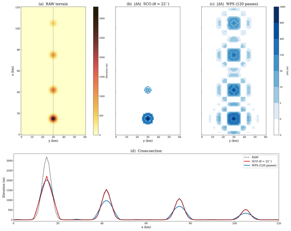
and the linear approximation θ_eff≈0.93 θ holds to within 0.1° over 18–26°. Local tightening can reduce the working bounds further. A field that fully satisfies the initial bounds has $S_{max,\mathrm{int}}\le {\mathit{\theta }}_{\mathrm{eff}}$, apart from numerical tolerance, but acceptance at the nominal angle θ does not establish convergence to those bounds. The idealised example in Fig. 1 illustrates the basic contrast: SCO modifies only the cones whose slopes violate the working bounds, whereas WPS smoothing alters all four. RAW denotes the unsmoothed reference terrain.

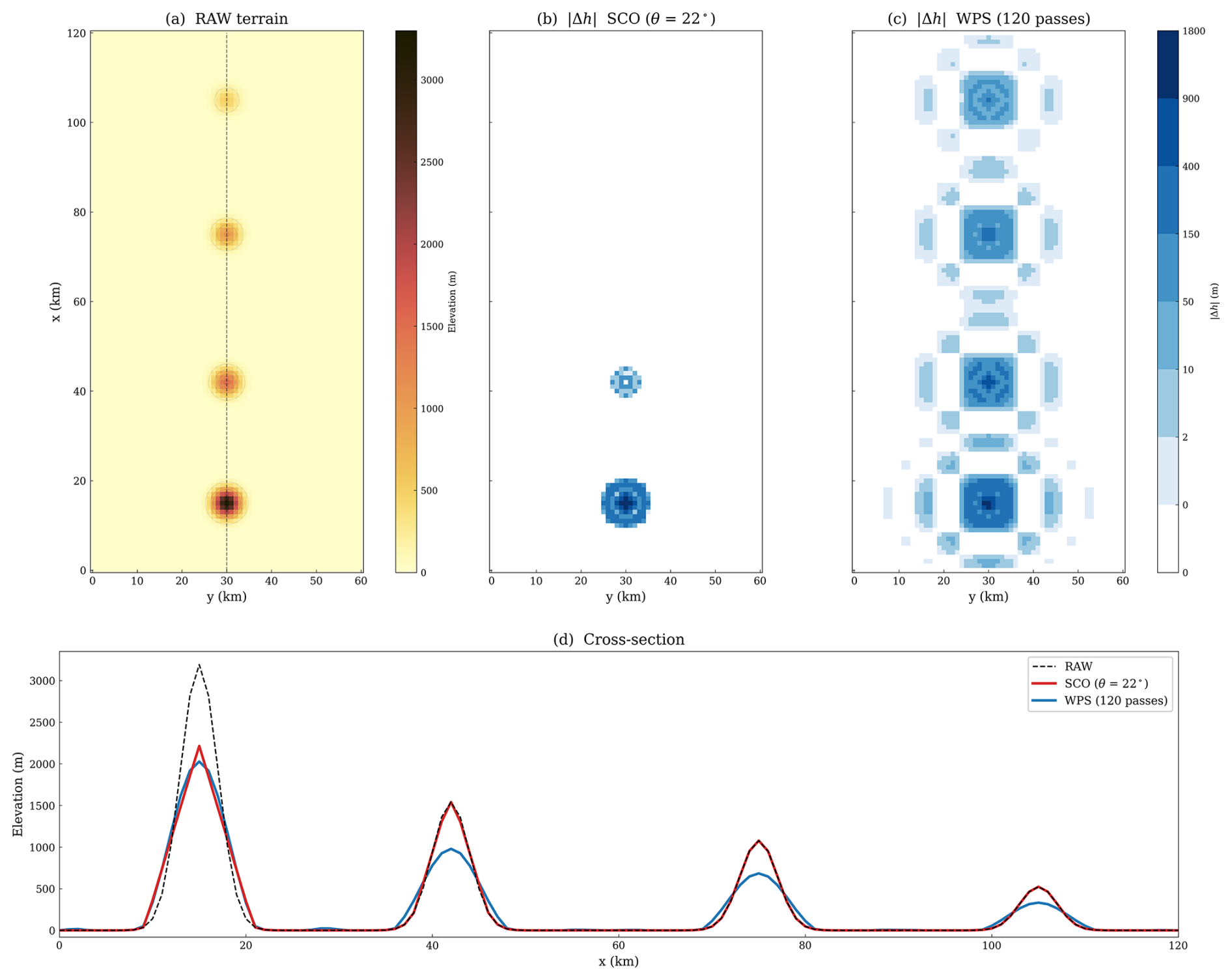
Figure 1 Idealised terrain fields used to contrast SCO and WPS smoothing. Four Gaussian cones (σ=2.0 km) with peak slopes of 43, 24, 18, and 9° are placed on a flat plain at Δx=1 km. The angle of the initial working bounds corresponding to θ=22° is θ_eff=20.5°. (a) RAW terrain; the dashed line marks the cross-section in (d). (b) Absolute elevation change $\left|\mathrm{\Delta }h\right|$ after SCO with θ=22°. (c) Absolute elevation change $\left|\mathrm{\Delta }h\right|$ after 120 passes of WPS smth-desmth_special. (d) Cross-section through the cone centres.

2.3 Iterative projection solver

Each grid point carries a mobility weight $w_{i,j}\in [\mathrm{0},\mathrm{1}]$ that controls how freely the solver may adjust its elevation. Water points receive w=0 and are never modified. The outermost r rows and columns are likewise frozen at w=0; across the next t rows and columns inward, a cosine taper raises w smoothly from 0 to 1. All remaining interior land points carry w=1. The fixed settings used here are r=3 and t=5.

Grid points with w>0.5 define the active interior. This threshold coincides with the midpoint of the cosine taper and marks the region over which $S_{max,\mathrm{int}}$ is evaluated and the outer acceptance test is applied. Boundary points (w≤0.5) may retain residual slope violations, but do not enter the outer acceptance test or local tightening. The inner monitor includes all neighbour pairs with $w_p+w_q>{\mathrm{10}}^{-\mathrm{6}}$, including pairs adjoining frozen points.

The solver sweeps four classes of neighbour pairs in sequence (horizontal, vertical, main diagonal, anti-diagonal) using a red–black decomposition for vectorised execution. For a neighbour pair (p,q), the working bound is $L_{pq}=(d_{pq}/\mathrm{\Delta }x)min(f_p,f_q)\mathrm{\Delta }{h}_{max}^{\left(\mathrm{0}\right)}$, where d_pq=Δx for cardinal pairs and $\sqrt{\mathrm{2}}\mathrm{\Delta }x$ for diagonal pairs. The local tightening factor f is initially 1. It changes the bound, whereas the mobility weight w determines how the correction is shared. When the height difference $\mathit{\delta }=h_q-h_p$ exceeds L_pq in magnitude and the pair is movable, the excess

$$\begin{array}{}\text{(4)}& e=\mathit{\delta }-\mathrm{sgn}\left(\mathit{\delta }\right)L_{pq}\end{array}$$

is redistributed according to the endpoint mobilities:

$$\begin{array}{}\text{(5)}& h_p\leftarrow h_p+e{\displaystyle \frac{w_p}{w_p+w_q}},h_q\leftarrow h_q-e{\displaystyle \frac{w_q}{w_p+w_q}}.\end{array}$$

When both endpoints share the same mobility the pair mean is conserved. When they differ, as in the transition zone, the more mobile endpoint absorbs the larger share and the pair mean shifts toward the less mobile point. Frozen points (w=0) never move.

An outer loop progressively tightens the local bound at each active interior point through the factor f_i,j:

$$\begin{array}{}\text{(6)}& \mathrm{\Delta }{h}_{max,i,j}=f_{i,j}\mathrm{\Delta }{h}_{max}^{\left(\mathrm{0}\right)}.\end{array}$$

For sweep s, the monitored quantity E_s is the largest positive pairwise exceedance $max\left(\right|h_q-h_p|-L_{pq},\mathrm{0})$ encountered over movable pairs during the sweep. The inner stopping conditions are E_s<0.1 m, stagnation, or the limit of 500 sweeps. Stagnation means $E_s\ge \mathrm{0.999}{E}_{s-\mathrm{1}}$ for three consecutive comparisons. Persistent exceedances beside the frozen boundary can trigger this exit before the active interior has fully converged.

After each inner solve, the outer acceptance test checks $S_{max,\mathrm{int}}\le \mathit{\theta }+\mathrm{0.01}$°. If it is not met, the factors at active interior points with $S_{i,j}>\mathit{\theta }$ are tightened as

$$\begin{array}{}\text{(7)}& f_{i,j}\leftarrow max\left(f_{i,j}\mathit{\beta }{\displaystyle \frac{\mathit{\theta }}{S_{i,j}}},f_{min}\right),\end{array}$$

where β=0.97 and $f_{min}=\mathrm{0.30}$ are fixed. The next inner solve uses the updated bounds. The outer loop ends on acceptance or after 10 rounds. The full pseudocode and parameter values are given in Appendix A2. All offline diagnostics and figures in this study use max_outer = 10, max_sweeps = 500, inner_tol = 0.1 m, and outer_tol_deg = 0.01°. These are also the module defaults in the released code, which users may adjust for other domains.

2.4 Offline diagnostics

The offline diagnostics quantify achieved slopes, the magnitude and extent of terrain modification, and retained small-scale terrain structure. The near-maximum count is the number of active interior points whose S_i,j falls within ε=0.2° below the member's own $S_{max,\mathrm{int}}$. It describes concentration in the slope distribution, not geographic clustering.

Terrain fidelity is characterised by the mean absolute elevation change, ${\mathrm{MAE}}_h=\langle |h_{\mathrm{new}}-h_{\mathrm{raw}}|\rangle$, over interior land points. The modified-area fraction is the proportion of those points where $|h_{\mathrm{new}}-h_{\mathrm{raw}}|>\mathrm{0.1}$ m. MAE_h measures the typical magnitude of elevation change. The modified-area fraction measures how widely those changes spread. Retained small-scale terrain structure is quantified by the root-mean-square (RMS) over interior land points of the unnormalised five-point second difference

$$\begin{array}{}\text{(8)}& L_{i,j}=h_{i+\mathrm{1},j}+h_{i-\mathrm{1},j}+h_{i,j+\mathrm{1}}+h_{i,j-\mathrm{1}}-\mathrm{4}{h}_{i,j}\end{array}$$

(in metres). On the uniform grid, this difference equals Δx² times the discrete Laplacian. Because it responds to second-order terrain structure, it distinguishes terrain fields with similar $S_{max,\mathrm{int}}$ but different small-scale content. Ridge-to-valley relief retention along cross-sections is defined as the ratio of the peak-to-valley elevation difference in the processed field to that in RAW.

3 Experimental design

3.1 Study region and model configuration

The test region is the southeastern Tibetan Plateau (Fig. 2), where raw discrete slope angles on a 1 km grid exceed 40° (Table 1). Two one-way-nested WRF-ARW v4.6.1 domains are used. The outer domain (D01) covers the eastern Tibetan Plateau margin and the Sichuan Basin on a 360×360 grid at 3 km spacing; the inner domain (D02) spans the steep plateau–basin transition on a 420×420 grid at 1 km spacing. Both domains use 54 vertical levels with a model top at 50 hPa and the hybrid terrain-following coordinate. D01 supplies the lateral boundary conditions for D02, with no feedback from D02 to D01. D01 terrain is fixed after one WPS smth-desmth_special pass; all terrain-treatment differences are confined to D02. Time steps were reduced for the WPS configurations as needed for stability (Fig. 3). With the parent-to-nest time-step ratio fixed at 3, these reductions also change the parent-domain integration.

Table 1 Terrain members with offline diagnostics and stability outcomes. The control parameter is the WPS pass count N or the SCO target angle θ. For SCO members, θ_eff is the angle corresponding to the initial working bounds (Sect. 2.2). “48 h” gives the reported integration outcome under the stated 48 h stability criterion and the member-specific configuration (Fig. 3). W1+SCO24 MAE_h is measured relative to its WPS01-smoothed input rather than to RAW, and its modified-area fraction is not directly comparable to the RAW-referenced values of the other members; neither quantity enters the cross-method comparison.

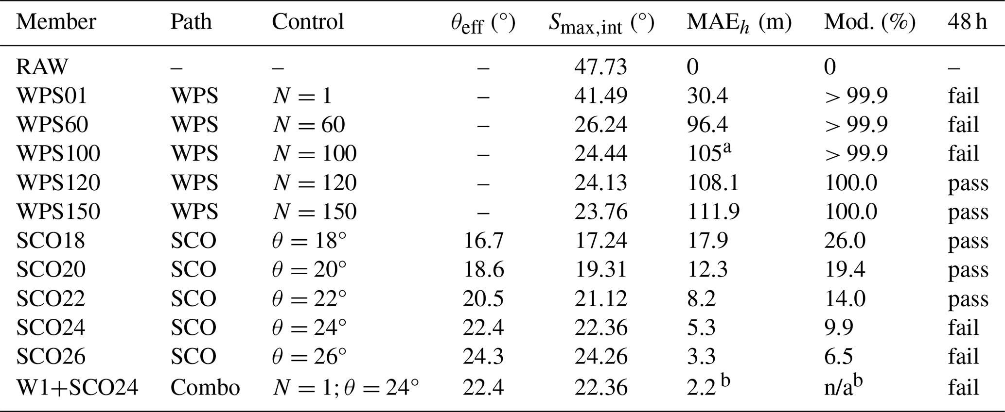
^a WPS100 MAE_h is rounded to the nearest integer. ^b W1+SCO24 MAE_h is measured relative to its WPS01-smoothed input, not relative to RAW; excluded from the cross-method comparison. n/a: not applicable.

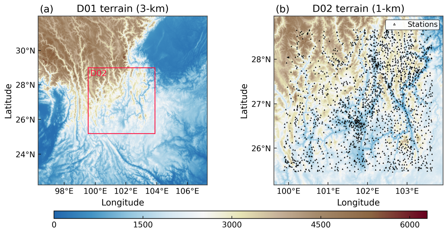
Figure 2 Model domains and observation network. (a) D01 terrain elevation (3 km grid spacing) with the D02 boundary marked. (b) D02 terrain elevation (1 km grid spacing) with the 927 surface stations used for near-surface verification.

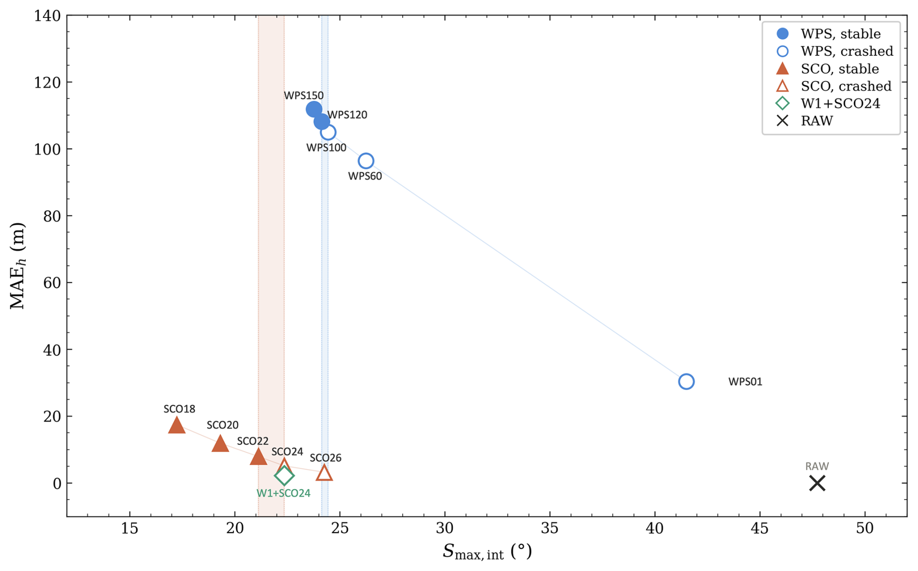
Figure 3 Terrain-member pathways in (MAE_h, $S_{max,\mathrm{int}}$) space. Filled symbols indicate stable members and open symbols indicate failed members. Shaded bands span the adjacent passing and failing candidates; the WPS interval also includes a change in time step. For W1+SCO24, MAE_h is referenced to its WPS01 input rather than RAW. Reported D01/D02 time steps: SCO and W1+SCO24, 18/6 s; WPS100, 15/5 s; WPS120 and WPS150, 12/4 s. WPS120 failed at 18/6 s and passed at 12/4 s.

All simulations are initialised at 00:00 UTC (Coordinated Universal Time) 18 July 2025 from the fifth-generation reanalysis (ERA5) of the European Centre for Medium-Range Weather Forecasts (Hersbach et al., 2020) and integrated for 48 h. Static terrain for the 1 km inner domain is built from the 30 m Advanced Spaceborne Thermal Emission and Reflection Radiometer (ASTER) Global Digital Elevation Model (GDEM; Tachikawa et al., 2011) by area averaging onto the model grid. The physics configuration is identical across all experiments: Thompson microphysics (Thompson et al., 2008), Rapid Radiative Transfer Model for general circulation models (RRTMG) radiation (Iacono et al., 2008), the Yonsei University (YSU) planetary boundary layer scheme (Hong et al., 2006), the revised Fifth-Generation Penn State/National Center for Atmospheric Research mesoscale model (MM5) Monin–Obukhov surface layer, Noah land surface model with multiparameterization options (Noah-MP) (Niu et al., 2011), and gravity-wave drag on D01 only. No cumulus parameterisation is used on either domain. A reference WRF namelist is provided in the code repository.

3.2 Terrain members and member selection

For the WPS pathway, smth-desmth_special is applied for N passes to the aggregated D02 terrain, and the member label gives the pass count. Five members are tested: WPS01, WPS60, WPS100, WPS120, and WPS150. SCO members are generated by applying the slope-constrained adjustment (Sect. 2.3) directly to the unsmoothed D02 terrain. Five members span θ=18 to 26° at 2° intervals, with the member label giving the target angle. All SCO members share the same solver settings (r=3, t=5, β=0.97, $f_{min}=\mathrm{0.30}$); only θ varies. RAW is retained as an offline reference. A control experiment, W1+SCO24, applies one WPS pass before SCO at θ=24° to test whether light pre-smoothing changes the stability outcome at fixed $S_{max,\mathrm{int}}$.

The cross-method comparison pairs the least-modified stable member from each method among the discrete candidates tested under their reported configurations and the same 48 h stability criterion. These selections are neither exact stability limits nor globally optimal terrain solutions. Members are not matched by slope or terrain cost, since neither method offers a natural counterpart at fixed values of these quantities. One additional stable member from each method enters the near-surface evaluation to gauge within-method sensitivity.

3.3 Observations and verification protocol

Near-surface verification uses hourly 10 m wind speed and 2 m temperature from 927 China Meteorological Administration (CMA) surface stations within the D02 interior (Fig. 2b). The denser local network improves spatial sampling in interior valleys, where terrain effects are expected to be strongest.

Stations within 30 grid points of the lateral boundaries are excluded to avoid relaxation-zone contamination, and each retained time series must contain at least 20 % valid observations during the 48 h window. At any given station, the terrain-height difference between members is much smaller than the model-minus-observation elevation offset, so systematic elevation bias largely cancels in the paired comparison. Model fields are bilinearly interpolated to station locations without elevation correction.

The final sample contains 44 200 wind pairs and 44 115 temperature pairs. Inter-member root-mean-square error (RMSE) differences are tested with a two-sided paired t-test across stations, each contributing one time-averaged RMSE value. The test does not account for spatial correlation among nearby stations, so the reported p values should be interpreted as approximate.

4 Results

4.1 Terrain modification and retained structure

Under the common 48 h stability criterion, SCO22 and WPS120 are the least-modified stable members among those tested for the two methods (Table 1). Their terrain costs differ by an order of magnitude. SCO22 modifies 14.0 % of interior land points with MAE_h=8.2 m; WPS120 modifies the entire domain and has MAE_h=108.1 m (Fig. 3).

SCO22 also retains far more small-scale terrain structure. Its RMS of the five-point second difference reaches 279.8 m, nearly six times the 47.9 m of WPS120. Cross-sections confirm the same pattern: SCO22 retains 97 %–99 % of the RAW ridge-to-valley relief along two representative transects, compared with 79 %–86 % for WPS120 (Fig. 4).

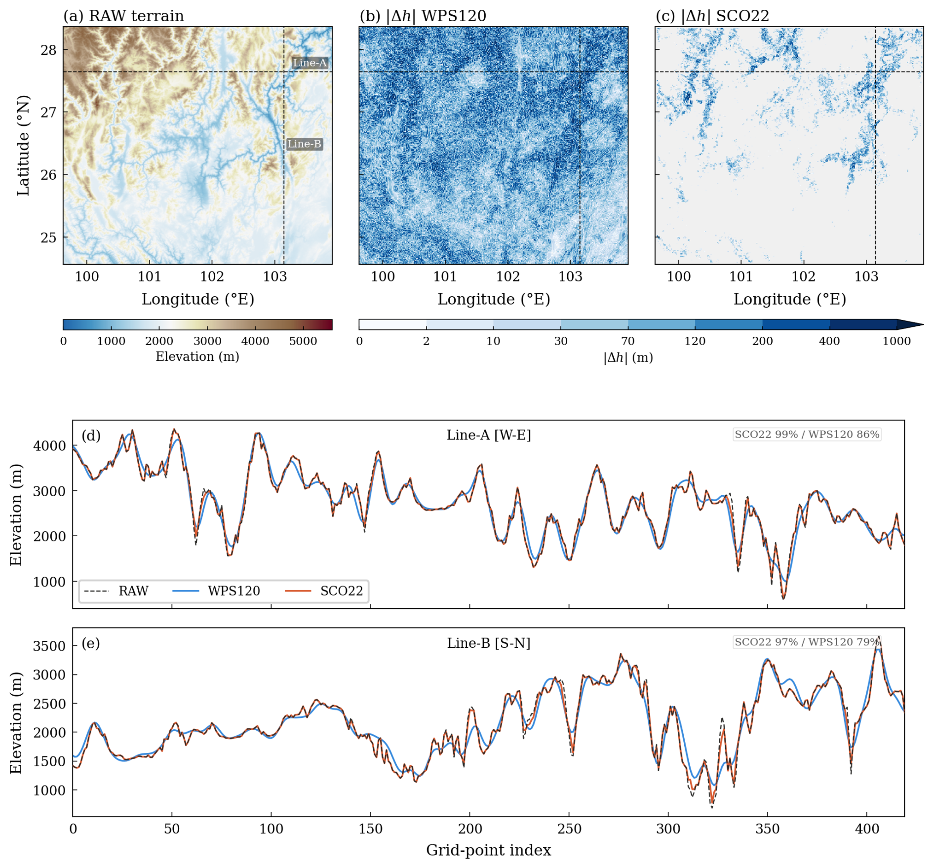
Figure 4 Terrain modification footprint and retained relief. (a) RAW terrain elevation with cross-section locations marked. (b) Absolute elevation change $\left|\mathrm{\Delta }h\right|$ for WPS120 and (c) for SCO22, shown on the same colour scale (0–1000 m). (d) West–east cross-section along Line-A (j=339) and (e) south–north cross-section along Line-B (i=346). Annotated percentages denote ridge-to-valley relief retained relative to RAW.

All SCO members attain the nominal target θ over the active interior (Fig. 5). The maxima for SCO24 and SCO26 lie close to θ_eff, whereas those for SCO18–SCO22 remain above it (Table 1; Fig. 5c). The latter fields pass the outer acceptance test without fully satisfying the tighter internal working bounds, consistent with the stagnation exit described in Sect. 2.3.

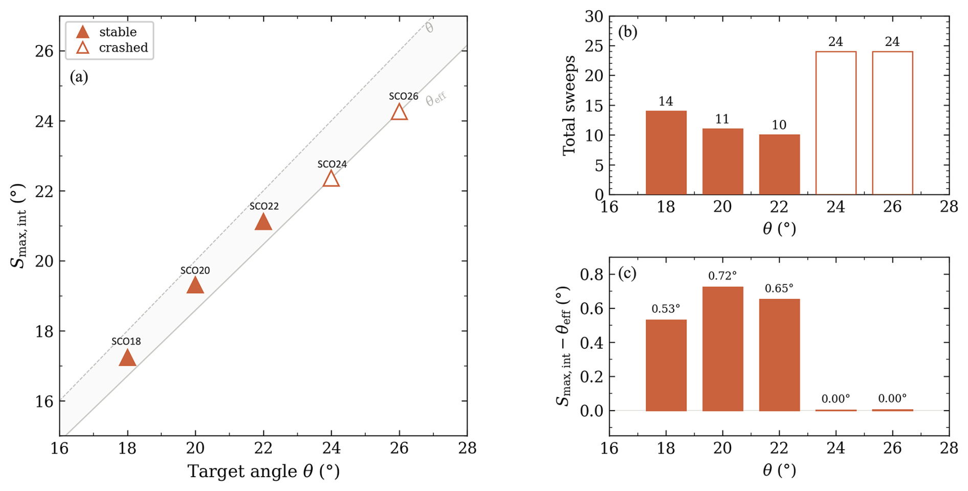
Figure 5 Target θ versus achieved $S_{max,\mathrm{int}}$ for SCO18–SCO26. (a) The solid line marks θ_eff and the dashed line θ; filled triangles indicate stable members and open triangles indicate failed members. (b) Total sweep count. (c) Angular difference $S_{max,\mathrm{int}}-{\mathit{\theta }}_{\mathrm{eff}}$ after the final outer round. The positive differences for SCO18–SCO22 distinguish attainment of the nominal target from convergence to the internal working bounds.

4.2 Diagnostics near the stability boundary

The WRF integrations with the unstable members terminated prematurely. Along the WPS pathway, WPS100 ($S_{max,\mathrm{int}}=\mathrm{24.44}$°) fails while WPS120 (24.13°) completes the full 48 h integration under the reported configurations (Table 1; Fig. 3). Along the SCO pathway, SCO24 (22.36°) fails and SCO22 (21.12°) passes, a sampled passing–failing gap of 1.24°. The selected stable members, SCO22 and WPS120, differ by 3.0° in peak slope.

At the domain scale, the slope fields of SCO22, SCO24, WPS100 and WPS120 differ sharply. Of the active interior points in SCO24, 15 359 fall within ε=0.2° below its own $S_{max,\mathrm{int}}$; WPS120 has only 4 (Table 2). The exceedance counts (Fig. 6b) illustrate the same contrast: SCO members drop steeply near their diagnosed maxima, whereas the WPS tail decays gradually over several degrees. Because repeated smoothing progressively lowers slopes, few WPS grid points remain near the residual peak. In the slope probability density functions (PDFs; Fig. 6a), the contrast takes a different form: the WPS distribution falls off gradually in the upper tail, with most grid points well below the peak, while SCO24 has a concentrated population near its working bound.

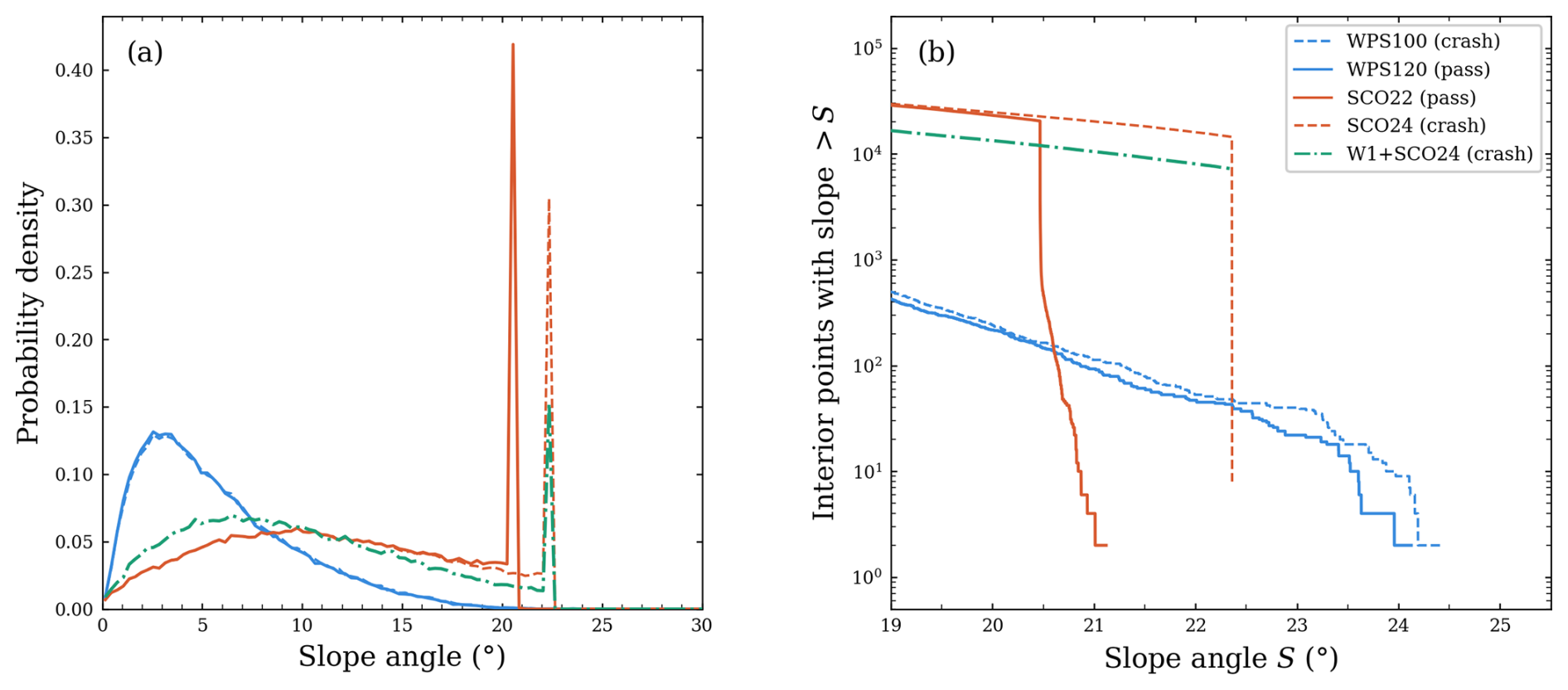
Figure 6 Slope distributions for members near the stability boundary. (a) Probability density functions for WPS100, WPS120, SCO22, SCO24, and W1+SCO24. (b) Exceedance counts: number of active interior grid points with discrete slope exceeding S, shown on a logarithmic vertical axis. The sharp drop-off in the SCO members reflects the slope-constrained adjustment; the gradual tail in the WPS members reflects the progressive nature of domain-wide smoothing.

Table 2 Diagnostics for selected members near the sampled passing–failing intervals. Near-maximum count is the number of active interior points within ε=0.2° below each member's own $S_{max,\mathrm{int}}$; it describes the slope distribution, not geographic clustering. Second-difference RMS is the RMS of the unnormalised five-point second difference in Eq. (8). Spectral retention is defined relative to RAW at the indicated wavelengths. Outcomes refer to the configurations in Fig. 3.

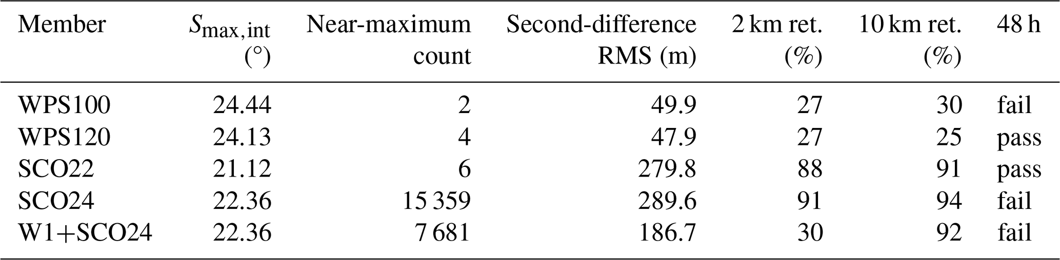
Figure 7 compares the local terrain around the reported failure site. Within this 41×41 neighbourhood, SCO24 retains small-scale ridge–valley structure and has 604 grid points above 22°. By contrast, WPS100 presents a narrow band of steep slopes against a smooth background, with only 23 grid points above 22°.

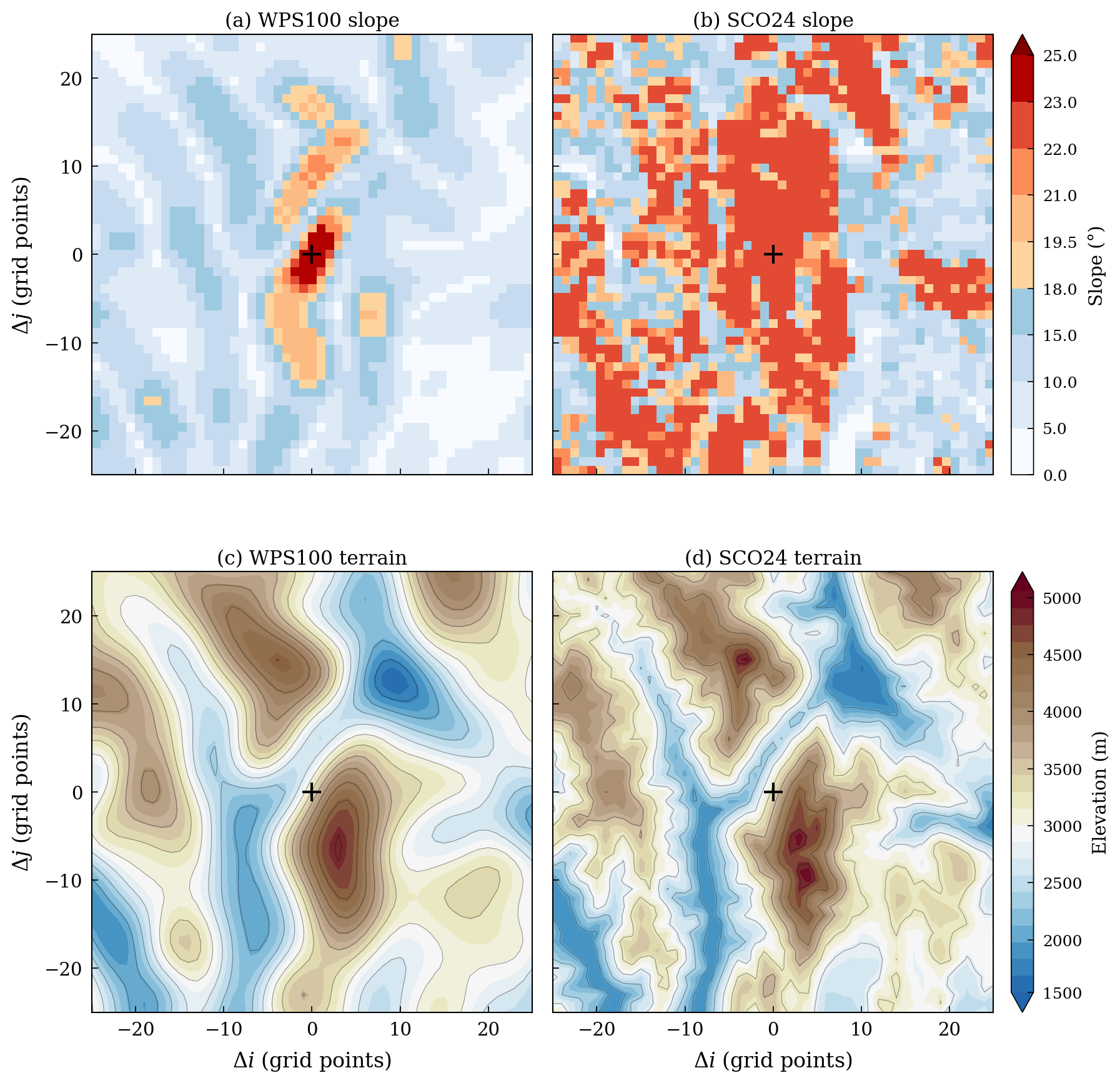
Figure 7 Local slope and elevation fields near the shared crash location (41×41 neighbourhood centred on i=50, j=291, 1-based). (a, b) Discrete slope S_i,j for WPS100 and SCO24. (c, d) Terrain elevation for the same members. The cross marks the failure site.

W1+SCO24 tests whether removing small-scale terrain structure at fixed $S_{max,\mathrm{int}}$ can produce a stable integration. One WPS pass applied before SCO at θ=24° lowers the second-difference RMS from 289.6 to 186.7 m and approximately halves the near-maximum count (from 15 359 to 7681), while holding $S_{max,\mathrm{int}}$ at 22.36° (Table 2). Row-mean spectra confirm that about 70 % of the power near 2 km wavelength is removed, while the 10 km band remains largely intact (Fig. 8). SCO24 and W1+SCO24 both fail. The tested pre-smoothing was therefore insufficient to restore stability under these settings.

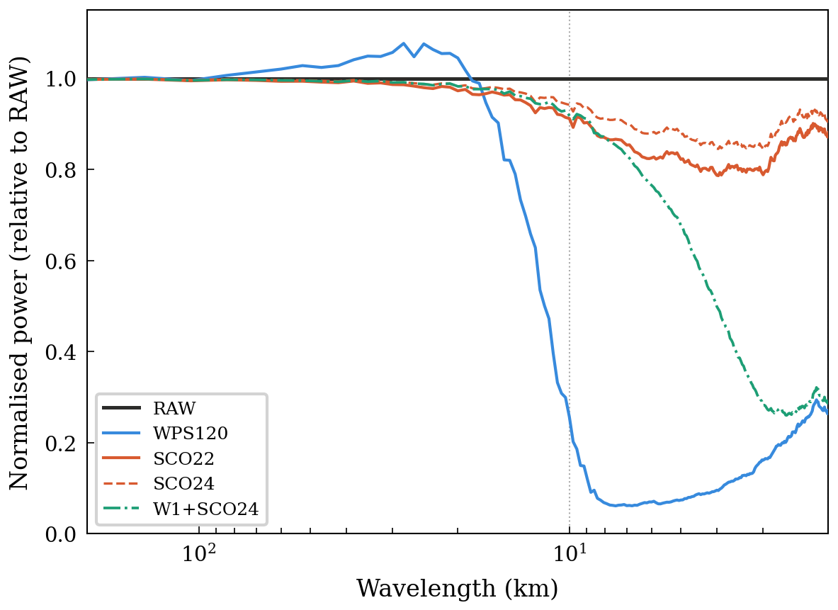
Figure 8 Row-mean terrain power normalised by RAW at each wavenumber for RAW, WPS120, SCO22, SCO24 and W1+SCO24. Wavelength is shown on a logarithmic horizontal axis. Vertical dotted lines mark 2 and 10 km.

Figure 8 shows SCO22 and SCO24 because they bracket the sampled SCO passing–failing interval; it also compares WPS120 and W1+SCO24. SCO22 and SCO24 retain most of the RAW power near 2 and 10 km, and SCO24 retains more than SCO22; WPS120 removes most of the power in those bands (Table 2). SCO is a nonlinear local adjustment, so its spectral response depends on terrain amplitude and structure, grid spacing and θ rather than on a fixed transfer function. In the tested sequence, lower θ increases terrain modification (Table 1). The slope distributions and second-order diagnostics show that the methods produce different terrain structures beyond the maximum slope. Those properties may influence numerical behaviour, but the present experiments do not isolate their effects.

4.3 Near-surface verification

Four stable members (WPS120, WPS150, SCO20, and SCO22) are evaluated against the 927-station network over the full 48 h period (Table 3). Comparing the two least-modified stable members, SCO22 produces lower errors for both variables: wind RMSE is lower by about 0.15 m s⁻¹ with a weaker positive bias, and 2 m temperature RMSE is lower by about 0.16 K (Table 3). The error differences between these successful configurations cannot be attributed to D02 terrain alone. The 2 m temperature bias reverses sign between the two members (±0.17 K) but at this magnitude it is too small to diagnose a systematic difference.

Table 3 Forty-eight-hour near-surface verification. RMSE denotes root-mean-square error. SCO20 and SCO22 show no detectable difference in wind RMSE (p=0.97) or in 2 m temperature RMSE (p=0.32) under the approximate two-sided paired t-test across stations (Sect. 3.3).

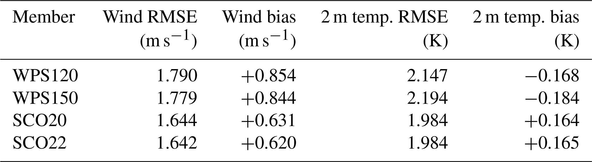
Within-method differences are much smaller. SCO20 and SCO22 show no detectable difference in wind and temperature RMSE under the approximate stationwise paired test (Sect. 3.3). The step from WPS120 to WPS150 changes scores only modestly. Because the comparison rests on a single 48 h case, these numbers are specific to the present domain and period.

5 Discussion

SCO meets the stability criterion on this domain with far less terrain alteration than WPS. WPS120 has a higher $S_{max,\mathrm{int}}$ than SCO24, and the two members' slope fields differ markedly in how many grid points lie near their respective maxima. The W1+SCO24 control shows that removing much of the small-scale structure while holding $S_{max,\mathrm{int}}$ fixed does not recover stability under the tested settings. The diagnostics examined here may not capture all terrain differences relevant to stability.

The diminishing returns of repeated smth-desmth_special passes compound the terrain-cost asymmetry between the two methods (Fig. 3). Small-scale terrain is removed much faster than the residual peak slope declines. Among the evaluated stable SCO members, SCO20 and SCO22 yield nearly identical forecast scores. A filter-based approach requires the user to choose a pass count, blending factor, or filter width and then inspect the resulting slope field. SCO prescribes θ first and uses the same variable to generate candidates, diagnose them offline, test for stability, and select the final member. On the 420×420 D02 grid used here, each SCO member is generated in under 10 s on a single central processing unit (CPU) core, so the entire five-member θ sweep completes in under a minute.

A practical workflow begins by diagnosing the raw terrain and generating a coarse sequence of θ values. Each field is checked offline for $S_{max,\mathrm{int}}$, residuals relative to its internal working bounds, and the magnitude and extent of terrain modification. Stability integrations with a fixed model configuration and time step then bracket the sampled passing–failing interval. The interval can be refined if needed, and the least-modified passing member is selected from those tested. The selection must be reassessed when the model configuration changes.

The focus of this study is not on forecast improvement through terrain modification, but on preserving terrain fidelity as far as possible while maintaining numerical stability. Greater retention of ridge–valley relief and terrain spectral content (Figs. 4 and 8) preserves more of the lower-boundary structure available to force local atmospheric flows. The hourly station evaluation quantifies bulk errors, whereas assessing the realism of resolved flow variability requires complementary diagnostics, as illustrated by Sheridan et al. (2023). Such variability was not evaluated here.

6 Conclusions

SCO prescribes the target slope angle θ as its primary user-facing parameter and applies local eight-neighbour terrain adjustments between geogrid and metgrid. The parameter provides a geometrically interpretable way to generate terrain candidates and organise stability tests. On the highly complex terrain of the southeastern Tibetan Plateau at 1 km grid spacing, the least-modified stable SCO member among those tested (SCO22) completes a 48 h integration with MAE_h=8.2 m and 86 % of interior land points unmodified, compared with MAE_h=108.1 m and 100 % modification for the least-modified stable WPS member (WPS120). SCO22 retains substantially more small-scale terrain structure than WPS120, while the near-boundary candidates show distinct upper-tail slope distributions. The sampled passing range is specific to the tested case and model configuration.

For the successful configurations, SCO22 also produces lower near-surface wind and temperature errors in this 48 h case. Whether this advantage holds across other domains and seasons remains to be tested. With each candidate terrain generated in seconds, SCO provides an efficient way to explore the balance between terrain retention and numerical stability. Curvature constraints and packaging SCO as an optional WPS component are possible extensions. The current implementation assumes uniform grid spacing, and extending the projection geometry to variable-resolution or unstructured meshes is a natural next step toward broader applicability.

Appendix A: Geometric scaling and algorithm summary

A1 Conservative scaling for locally planar terrain

For a locally planar surface with gradient g=∇h, the neighbour-pair ratio in a unit direction u is $|h_q-h_p|/d_{pq}=|\mathit{g}\cdot \mathit{u}|$. Let 𝒰₈ contain the unit vectors along the eight sampled directions. They are separated by $\mathit{\pi }/\mathrm{4}$, so one lies within $\mathit{\pi }/\mathrm{8}$ of the gradient direction. Hence

$$\begin{array}{}\text{(A1)}& \underset{\mathit{u}\in {\mathcal{U}}_{\mathrm{8}}}{max}|\mathit{g}\cdot \mathit{u}|\ge \left|\mathit{g}\right|\cos (\mathit{\pi }/\mathrm{8}).\end{array}$$

If all sampled ratios are bounded by $\tan \mathit{\theta }\cos (\mathit{\pi }/\mathrm{8})$, then $\left|\mathit{g}\right|\le \tan \mathit{\theta }$. The corresponding elevation-difference bounds are $\mathrm{\Delta }x\tan \mathit{\theta }\cos (\mathit{\pi }/\mathrm{8})$ for cardinal pairs and $\sqrt{\mathrm{2}}$ times this value for diagonal pairs. The common scaling tightens both sets of bounds conservatively for any orientation of a plane; it does not remove the stencil's directional anisotropy. The angle of the initial pairwise bounds is θ_eff in Eq. (3).

A2 Pseudocode

The pseudocode below summarises the algorithm with the parameter values used for the terrain members analysed in this paper.

Algorithm A1 SCO v1.0.

Input: h(n_x,n_y) terrain elevation (m); landmask(n_x,n_y); Δx grid spacing (m); θ target slope angle (°); $r=\mathrm{3},t=\mathrm{5}$ frozen-rim and transition widths; β=0.97, $f_{min}=\mathrm{0.30}$, max_outer=10, max_sweeps=500, inner_tol=0.1 m, outer_tol_deg=0.01°

Output: h(n_x,n_y) adjusted terrain elevation; nominal-target acceptance flag

1. Compute base cardinal bound: $\mathrm{\Delta }{h}_{max}^{\left(\mathrm{0}\right)}\leftarrow \mathrm{\Delta }x\cdot \tan \left(\mathit{\theta }\right)\cdot \cos (\mathit{\pi }/\mathrm{8})$

2. Build mobility-weight field w(n_x,n_y):

w=0 where landmask<0.5

[water]

w=0 in outermost r rows and columns

[frozen rim]

w=cosine taper across next t rows and columns

[transition zone]

w=1 elsewhere

[interior land]

3. Initialise tightening factors: $f(i,j)\leftarrow \mathrm{1}$ for all (i,j)

4. Define active interior mask: $\mathrm{interior}\leftarrow (w>\mathrm{0.5})$; set acceptance flag to false

5. for round =1 to max_outer do

5a. Update local bounds: $\mathrm{\Delta }{h}_{max}(i,j)\leftarrow f(i,j)\cdot \mathrm{\Delta }{h}_{max}^{\left(\mathrm{0}\right)}$

Initialise E_prev←∞, c←0

5b. for sweep s=1 to max_sweeps do

Set E_s←0

for each pair class (horiz., vert., main diag., anti-diag.) do

for each red–black subset of pairs (p,q) do (vectorised)

$L_{pq}\leftarrow min\left(\mathrm{\Delta }{h}_{max}\right(p),\mathrm{\Delta }{h}_{max}(q\left)\right)$ [$\times \sqrt{\mathrm{2}}$ for diag.]

$\mathit{\delta }\leftarrow h\left(q\right)-h\left(p\right)$

if $\left|\mathit{\delta }\right|>L_{pq}$ and $w\left(p\right)+w\left(q\right)>{\mathrm{10}}^{-\mathrm{6}}$ then

$e\leftarrow \mathit{\delta }-\mathrm{sgn}\left(\mathit{\delta }\right)\cdot L_{pq}$

$E_s\leftarrow max(E_s,max|e\left|\right)$

$h\left(p\right)\leftarrow h\left(p\right)+e\cdot w\left(p\right)/\left(w\right(p)+w(q\left)\right)$

$h\left(q\right)\leftarrow h\left(q\right)-e\cdot w\left(q\right)/\left(w\right(p)+w(q\left)\right)$

if E_s≥0.999E_prev then $c\leftarrow c+\mathrm{1}$; else c←0

Set E_prev←E_s

if E_s<inner_tol or c≥3 then exit sweep loop

5c. Diagnose S(i,j) and $S_{max,\mathrm{int}}$ from updated h over interior points

5d. if $S_{max,\mathrm{int}}\le \mathit{\theta }+\mathrm{outer}\mathrm{\_}\mathrm{tol}\mathrm{\_}\mathrm{deg}$ then set acceptance flag to true and exit outer loop

5e. for each interior point where $S(i,j)>\mathit{\theta }$ do

$f(i,j)\leftarrow max\left[f\right(i,j)\cdot \mathit{\beta }\cdot \mathit{\theta }/S(i,j),f_{min}]$

6. return h and acceptance flag

Within each red–black subset, pairwise differences are evaluated before the endpoint contributions are accumulated. Pairs adjoining frozen points enter the inner monitor when at least one endpoint is movable; points outside the active interior do not enter the outer acceptance test or local tightening.