GPU-accelerated three-dimensional variational data assimilation with automatic differentiation for WRF-Chem

This study developed a PyTorch-based three-dimensional variational (3DVar) data assimilation system (PY3DVar) for the Weather Research and Forecasting model coupled to Chemistry (WRF-Chem), which integrates automatic differentiation (AD) to replace traditional manual gradient derivation and adopts Graphics Processing Unit (GPU) acceleration for high computational efficiency. PY3DVar enables the simultaneous assimilation of gaseous pollutants (SO₂, NO₂, CO, O₃) and particulate matter (PM_2.5, PM₁₀) and supports flexible deployment on both Central Processing Unit (CPU) and GPU computing platforms. Idealized tests were first conducted to verify the physical consistency of the assimilation system. Twenty consecutive real-case assimilation experiments, each followed by a 24 h forecast, were then conducted to assess computational performance and efficiency, benchmarked against the classic Fortran-based 3DVar system (FT3DVar) using CPU parallelization. The results of the idealized tests show PY3DVar effectively propagates observation information, generating increment fields consistent with FT3DVar. Long-term real-case experiments further verify that the two assimilation systems achieve nearly identical analysis accuracy for chemical initial fields. On the GPU platform, PY3DVar achieves an average assimilation time of 1.2 s, representing a 26.2-fold speedup compared to FT3DVar on 64 CPU cores (32.7 s). Parallel scalability tests across 1, 2, 4, 8, 16, 32 and 64 CPU cores reveal that FT3DVar runs faster per iteration across all core counts. Consequently, FT3DVar achieves shorter total assimilation time on 1, 2, 4 and 16 cores, whereas PY3DVar outperforms it at 8, 32 and 64 cores, owing to its intrinsically fewer required iterations for convergence. The average 24 h forecast results show that the improved initial fields have sustained positive effects on short-term forecasts: the improvements persist for over 24 h for SO₂, CO, PM_2.5, and PM₁₀, and for over 6 h for NO₂ and O₃. These results demonstrate that PY3DVar delivers substantially faster assimilation than FT3DVar while maintaining equivalent analysis accuracy, offering an efficient and practical solution for operational atmospheric chemical data assimilation.

1 Introduction

Air quality models (AQMs) are crucial tools for atmospheric pollution simulation and forecasting (Li et al., 2013; Wang et al., 2022; Gao et al., 2024). Errors in initial conditions can degrade model performance, particularly within the early hours of simulation, leading to significant biases in short-term forecasts. Data assimilation (DA) combines multi-source observations, such as those from surface stations and satellites, with model background fields through statistically derived weighting to produce an optimal analysis field. This technique effectively improves the initial conditions of numerical models and has become a core method for enhancing simulation accuracy in both research and operational forecasting (Engelen et al., 2009; Ma et al., 2025).

Compared to the long-standing development of meteorological data assimilation, atmospheric chemical data assimilation started relatively late, and its theoretical framework and operational applications are still under continuous improvement. Early explorations in atmospheric chemical data assimilation were largely constrained by limitations in observational capabilities and the difficulty of simulating complex aerosol compositions. Consequently, research initially focused on gaseous precursors like SO₂, NO₂, O₃ and typical key chemical components like HNO₃ with clear chemical reaction mechanisms and mature simulation schemes. In contrast, the assimilation of particulate matter (PM) components was less common due to the high complexity of their sources and physicochemical mechanisms. In earlier work, Austin (1992) assimilated Limb Infrared Monitor of the Stratosphere (LIMS) satellite measurements of HNO₃ and O₃ into a 2D chemical model, effectively identifying and correcting systematic biases in the original chemical model, significantly improving the analysis accuracy of stratospheric chemical composition, and demonstrating the key role of four-dimensional assimilation in refining chemical models. Elbern et al. (1997) used the Second-Generation Regional Acid Deposition Model (RADM2) gas-phase chemical mechanism and a variational method to assimilate ozone observations, successfully optimizing the initial concentrations of its precursors NO_x and volatile organic compounds (VOCs), and enabling quantitative analysis of ozone chemical sensitivity. Frydendall et al. (2009) developed a data assimilation algorithm based on statistical interpolation and coupled it with the Danish Eulerian Operational Model (DEOM), conducting assimilation studies on surface ozone and effectively improving forecast performance by optimizing assimilation parameters.

With advancements in observational technology and the continuous improvement of atmospheric chemistry modeling systems, the focus of atmospheric chemical data assimilation has gradually expanded to include particulate pollutants with more complex compositions and sources. In the early stages, owing to the limited simulation capability for aerosol physicochemical processes, assimilation studies mainly focused on adjusting total mass concentrations, such as PM_2.5 and PM₁₀, to improve model performance. For example, Denby et al. (2008) applied both Statistical Interpolation (SI) and ensemble Kalman filter (EnKF) data assimilation methods to an atmospheric chemistry model. They found that both methods significantly corrected the model's systematic underestimation of PM₁₀ concentration, with the SI method reducing the root mean square error (RMSE) of daily average concentration from 16.7 to 9.2 µg m⁻³, and noted that the improvement from SI was significantly better than that from EnKF. Tombette et al. (2009) used the optimal interpolation (OI) method to assimilate surface PM₁₀ observations from France into a regional chemical transport model, effectively enhancing the short-term forecast accuracy of total aerosol mass (PM_2.5 and PM₁₀) across Europe, demonstrating the potential application of this method in operational forecasting.

As a core method in data assimilation, the 3DVar approach statistically combines observations with model background fields to derive improved initial conditions by minimizing a prescribed cost function (Lorenc, 1986; Parrish and Derber, 1992). Although more advanced methods such as four-dimensional variational (4DVar) and hybrid ensemble-variational assimilation have been developed for global operational systems, 3DVar remains widely used in regional and chemical data assimilation applications owing to its computational efficiency, implementation simplicity, and robust performance (Jiang et al., 2013; Seo and Kim, 2023; Chen et al., 2024; Zhou et al., 2025). Pagowski et al. (2010) introduced surface ozone and fine particulate matter (PM_2.5) observations into the WRF-Chem model using the GSI (Grid-point Statistical Interpolation) 3DVar system. Results showed that while assimilation significantly reduced forecast errors, these errors grew rapidly in the early forecast hours. With the advancement of observational techniques and the refinement of model mechanisms, simply correcting total aerosol mass often fails to fundamentally optimize the simulation of its internal chemical composition. The target variables for aerosol assimilation are shifting from total mass concentration towards a multivariate system encompassing key chemical components such as sulfate, nitrate, and organic carbon. Li et al. (2013) integrated a 3DVar algorithm with the WRF-Chem model employing the Model for Simulating Aerosol Interactions and Chemistry (MOSAIC) aerosol scheme. By assimilating PM_2.5 observations, they achieved a comprehensive analysis of the concentrations and size distributions of eight key species, including black carbon, organic carbon, sulfate, and nitrate, significantly improving the simulation and forecast accuracy of these components. Jiang et al. (2013) implemented the assimilation of PM₁₀ observations using the 3DVar method, providing an improved initial field for the WRF-Chem model by optimizing various aerosol components. However, the assimilation effect diminished rapidly due to vertical mixing and advective processes, highlighting the importance of optimizing the aerosol vertical initial state. By designing various assimilation scenarios, Zang et al. (2016) confirmed that introducing aircraft-measured aerosol data into traditional surface-based aerosol data assimilation significantly optimized aerosol mass concentration, vertical distribution, and chemical composition. They also found that the forecast skill improvement from vertical observations lasted longer than that from surface data, underscoring the important influence of vertical resolution on forecast performance. Apart from experiments focusing on different observation types and pollutants, studies have optimized the intrinsic mathematical formulation of 3DVar algorithms. From a methodological perspective, Key et al. (2025) revealed the mathematical connection between 3DVar and Gaussian process regression, offering an alternative pathway for scalable assimilation computation.

Despite continuous improvements in assimilation algorithms and observation sources, traditional Fortran-based 3DVar systems still face prominent computational bottlenecks in modern high-resolution chemical assimilation scenarios. As observational data grow in volume and diversity, model resolutions become finer, and the number of simulated chemical species continues to expand, the state vector and matrix dimensions in atmospheric chemistry assimilation have increased substantially (Liang et al., 2020; Wang et al., 2022). The incorporation of satellite-derived aerosol optical depth and extinction profiles has proven effective for constraining the three-dimensional distribution of pollutants (Zhang et al., 2011; Chen et al., 2017; Ye et al., 2022; Wang et al., 2022). However, these observations require complex observation operators and their adjoints, which further compounds the computational challenge (Liang et al., 2020; Ye et al., 2021). These factors impose a heavy computational burden on traditional Fortran-based assimilation systems, prolonging assimilation time and challenging their ability to meet the timeliness requirements of operational air quality forecasting. In recent years, emerging high-performance computing techniques and PyTorch-based tensor computing frameworks have provided promising solutions to relieve the computational bottlenecks and tedious manual coding burden of traditional Fortran-based 3DVar systems (Boudier et al., 2023; De Luca et al., 2021; He et al., 2025). In parallel, modern deep learning (DL) frameworks such as PyTorch provide tensor-based computation and AD capabilities that are well suited to the matrix-dominated operations in variational data assimilation. Closely related to this study, Cheng et al. (2025) developed TorchDA, a Python package that implements multiple assimilation algorithms including 3DVar within PyTorch, demonstrating the feasibility of building variational assimilation systems in DL frameworks. However, TorchDA was demonstrated primarily on low-dimensional Lorenz models, and its applicability to full-scale atmospheric chemistry assimilation with three-dimensional grids and multiple species has not been established. Beyond updating classical algorithms, numerous full data-driven methods have been proposed to augment or replace components of traditional assimilation, such as using neural networks as ensemble surrogates (Chattopadhyay et al., 2023), adopting learned priors to replace background error covariance (Beauchamp et al., 2025), and constructing end-to-end frameworks that eliminate explicit observation operators (Xu et al., 2025). Although satisfactory computational efficiency, most existing fully data-driven assimilation methods are validated only under idealized low-dimensional experimental conditions. Meanwhile, their inherent black-box characteristic leads to poor physical interpretability and limited generalization ability. Such drawbacks not only hinder diagnostic analysis of pollution formation and evolution mechanisms, but also bring potential risks for reliable operational forecasting applications.

Overall, current atmospheric chemical data assimilation still faces a clear trade-off: traditional Fortran-based 3DVar owns rigorous physical basis and full mathematical traceability but suffers from low computational efficiency and tedious manual coding; pure DL-based assimilation achieves fast computation but sacrifices physical interpretability and practical robustness. To fill this research gap and balance reliable physical constraints and high computational performance, this study develops a novel PyTorch-based 3DVar assimilation system. The proposed framework inherits the complete classical 3DVar variational optimization theory without modifying underlying physical equations, guaranteeing transparent physical meaning and traceable gradient calculation throughout the assimilation workflow. Benefiting from native PyTorch AD and hardware-accelerated tensor parallel computing, the new system avoids manual adjoint programming and supports flexible deployment on both CPU and GPU hardware. Meanwhile, compared with fully black-box DL assimilation methods, it retains all physical constraints of traditional variational assimilation. This study finally conducts comprehensive contrast experiments between the newly built PY3DVar system and the traditional manually coded FT3DVar, focusing on computational efficiency, parallel scalability and assimilation analysis performance for multiple conventional air pollutants including SO₂, NO₂, CO, O₃, PM_2.5, and PM₁₀.

2 Model, data, and methodology

2.1 Air quality model

The WRF-Chem model was jointly developed by the National Center for Atmospheric Research (NCAR), the National Oceanic and Atmospheric Administration (NOAA), and other institutions (Grell et al., 2005; Fast et al., 2006). Its core strength lies in the fully online, bidirectional coupling between meteorological and chemical fields, enabling a precise description of pollutant transport, transformation, and removal under complex meteorological conditions. The meteorological fields drive the spatiotemporal distribution and transformation of chemical species through physical processes such as dynamic advection, turbulent diffusion, and dry/wet deposition. In turn, the chemical fields can feedback on meteorological elements through mechanisms like aerosol radiative forcing and cloud condensation nuclei effects. This online coupling ensures spatiotemporal consistency and physical compatibility between atmospheric dynamic processes and chemical transformations.

The WRF-Chem (version 3.5) used in this study integrates the Aerosol Module 5 (AERO5) from the Community Multiscale Air Quality Modeling System (CMAQ) and employs the Statewide Air Pollution Research Center 1999 (SAPRC-99) gas-phase chemical mechanism (Carlton et al., 2010; Carter, 2000; Li et al., 2010, 2011a, b, 2012). Through over two decades of development, this model incorporates advanced chemical reactions and processes crucial for atmospheric particulate formation. For example, it includes irreversible aqueous-phase processes of glyoxal and methylglyoxal on particle surfaces, which improves the simulation of secondary organic aerosol (SOA) over China (Xing et al., 2019). A parameterization for heterogeneous nitrous acid (HONO) processes has been implemented, enhancing the model's capability to simulate atmospheric oxidizing capacity and SOA (Feng et al., 2005, 2016). The suppression effect of organic coatings on the heterogeneous hydrolysis uptake of dinitrogen pentoxide (N₂O₅) is also parameterized, leading to better simulation of nitrate aerosols. Furthermore, the model incorporates sulfate formation via transition-metal catalysis and Criegee intermediate reactions, improving sulfate simulation. Additionally, a module accounting for aerosol–radiation–photolysis interactions has been developed, enabling assessment of aerosol–cloud interactions, radiative effects of brown carbon aerosols, and direct and indirect effects of various aerosol components.

In this study, a single-domain configuration with 210 (west–east) × 168 (south–north) grid points at 27 km horizontal resolution and 34 vertical layers was employed. The vertical layers follow a terrain-following coordinate with higher resolution near the surface that gradually decreases with altitude, extending from the surface to approximately 20 km. The domain-averaged height corresponding to each vertical level is illustrated in Fig. 3, which mainly presents the vertical distribution of background error standard deviation. The simulation domain covers most of China and surrounding regions, as shown in Fig. 1.

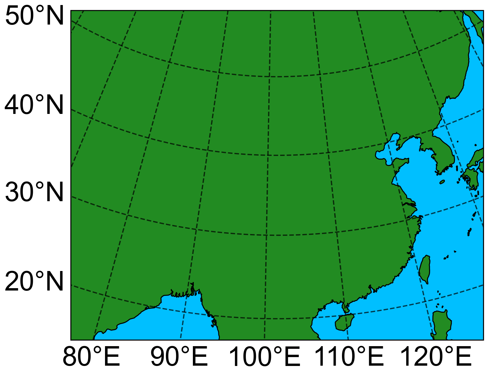
Figure 1 Distribution of the WRF-Chem simulation domain.

2.2 Data

The meteorological fields for the WRF-Chem model were driven by the NCEP Final Operational Global Analysis (FNL, https://doi.org/10.5065/D6M043C6, National Centers for Environmental Prediction et al., 2000) data, which has a horizontal resolution of 1° × 1° and a temporal resolution of 6 h. Provided by NCAR and NCEP, the FNL dataset assimilates multi-source global observations from surface stations, radiosondes, satellites, etc. It supplies physically consistent meteorological fields and serves as crucial input for generating reliable initial and boundary conditions for the model. This dataset has been widely used in various mesoscale numerical simulations.

Anthropogenic emissions were derived from the 2013 Multi-resolution Emission Inventory for China (MEIC, http://meicmodel.org.cn, last access: 20 October 2026), provided by Tsinghua University (Tong et al., 2020; Zheng et al., 2021). This inventory has a spatial resolution of 6 km, covers most regions of China, and includes emission data for the gaseous pollutants and aerosol precursors required in this study.

Chemical boundary conditions for the WRF-Chem model were obtained from the Whole Atmosphere Community Climate Model (WACCM, https://www.acom.ucar.edu/waccm/download.shtml, last access: 20 October 2026) data released by NCAR. This dataset provides the global spatiotemporal distribution of various chemical components, including ozone and aerosol precursors, ensuring reasonable atmospheric chemical boundary conditions for the regional air quality simulations.

Observation data were sourced from the China National Environmental Monitoring Centre (CNEMC, http://www.cnemc.cn/en/, last access: 20 October 2026), primarily comprising hourly surface concentrations of major air pollutants: SO₂, NO₂, CO, O₃, PM_2.5, and PM₁₀. The locations of observation sites follow the distribution described in He et al. (2025). To evaluate the assimilation performance, observations are divided into assimilation and independent validation datasets following Hu et al. (2022). Considering distinct missing-value characteristics among different pollutants, the station split was performed independently for each of the six pollutants and executed on a daily basis, using the observations at the assimilation start time (00:00 UTC) as the basis. The partitioning procedure for an individual pollutant is described as follows. First, invalid missing records of the target pollutant at 00:00 UTC are removed, and the remaining valid stations are mapped onto model grids. If only one valid station is present within a grid cell, it is assigned to the assimilation set. When two or more valid stations exist in one grid cell, one station is randomly selected for the independent validation set, and the rest are assigned to the assimilation set. After the station assignment for each pollutant at 00:00 UTC is completed, all 25 time steps of the forecast period (from 00:00 UTC of the current day to 00:00 UTC of the next day) share the same station assignment. Assimilation is performed only at the initial forecast time, and the subsequent time steps of the forecast period are used solely for forecast verification. For later hours, valid measurements from stations belonging to the validation set are treated as independent validation samples. Observations from stations outside the corresponding validation sets are marked as missing and are not used for validation.

2.3 Control variable design

The WRF-Chem model employed in this study incorporates aerosol variables that encompass a variety of fine and coarse particle components. The fine particle components include: elemental carbon (ECJ), ammonium (NH₄AJ), sulfate (SO₄AJ), nitrate (NO₃AJ_A/B), organic aerosols (ORGAJ, ORGBAJ, SOA_RXT_G/M), nine categories of secondary organic aerosols generated from the semi-volatile gases of primary organic aerosol (CPO1AER–CPO9AER), chloride (CLAJ), and accumulation-mode fine particles (P25AJ), among others. The coarse particle components include: dust (DUST_1–DUST_5), anthropogenic coarse aerosol (ANTHA), and coarse-mode soil-derived particles (SOILA). Furthermore, the model also includes gaseous pollutants such as SO₂, NO₂, CO, and O₃. The fine particle components listed above collectively constitute PM_2.5, while the addition of the coarse particle components (DUST_1–DUST_5, ANTHA, and SOILA) forms the complete PM₁₀ composition.

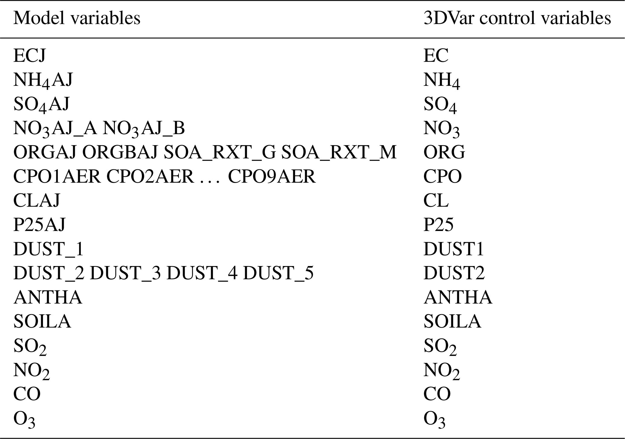
Using all aerosol species directly as control variables would provide detailed compositional resolution but at the cost of substantially increased computational scale, storage demands, and reduced efficiency. To balance assimilation accuracy with computational cost, this study merges specific components based on their physicochemical properties and particle size characteristics: the dual nitrate components are merged into a single variable; the four organic aerosol components are combined into one group; the nine secondary organic aerosols originating from semi-volatile primary organic gases are uniformly merged; the dust components are optimally merged according to particle size differences – DUST_1 is retained as an independent control variable, while DUST_2 to DUST_5 are merged into a single variable. Through this merging process, the number of aerosol control variables is reduced to 12. Gaseous pollutants (SO₂, NO₂, CO, O₃) are directly used as control variables for assimilation. Consequently, the assimilation system constructed in this study utilizes a total of 16 control variables. Table 1 provides the detailed mapping between the WRF-Chem model variables and the 3DVar control variables.

Table 1 Mapping between WRF-Chem model variables and 3DVar control variables.

2.4 3DVar assimilation theory

The 3DVar method is based on probability and statistical theory, treating both the simulated background field and observations as useful information containing errors. This method constructs a cost function that incorporates the weighted errors of the background field and the observations, and seeks the state that minimizes this function, known as the analysis field. Statistically, this analysis field is considered the optimal estimate of the true atmospheric state. The 3DVar cost function is:

$$\begin{array}{}\text{(1)}& \begin{array}{rl}J\left(\mathit{x}\right)& ={\displaystyle \frac{\mathrm{1}}{\mathrm{2}}}(\mathit{x}-{\mathit{x}}_{\mathrm{b}}{)}^{\mathrm{T}}{\mathbf{B}}^{-\mathrm{1}}\left(\mathit{x}-{\mathit{x}}_{\mathrm{b}}\right)\\ & +{\displaystyle \frac{\mathrm{1}}{\mathrm{2}}}(\mathbf{H}\mathit{x}-\mathit{y}{)}^{\mathrm{T}}{\mathbf{R}}^{-\mathrm{1}}\left(\mathbf{H}\mathit{x}-\mathit{y}\right)\end{array}\end{array}$$

where x is the analysis field, representing the set of control variables at all grid points in the model. Its dimensionality is jointly determined by the number of control variables, vertical layers, and horizontal grid points. x_b is the background field, provided by the WRF-Chem model simulation, and has the same dimensions as x. B is the background error covariance matrix, which describes the magnitude and spatial structure of the uncertainties in the background field. H is the observation operator that maps from model space to observation space. Since only surface in-situ observations are assimilated, H consists solely of horizontal bilinear interpolation from the model surface level to the observation locations, without any vertical interpolation. y is the observation vector, containing the assimilated observations, with dimensions of Obs_Station×6, where Obs_Station represents the number of valid observation sites, and 6 corresponds to the six types of pollutants. R is the observation error covariance matrix, representing the uncertainty of the observational data, with dimension matching the number of elements of the observation vector y. Following Li et al. (2013), the observational error standard deviation in this study is set to half of the background error standard deviation.

The background error covariance matrix B has a very large dimension. Storing and performing iterative computations with it directly would pose serious challenges to memory and computational efficiency. To optimize the solution of the cost function, this study adopts a classic preconditioning framework for variational data assimilation, factorizing and structurally simplifying the B matrix (El Akkraoui et al., 2013; Li et al., 2013). The specific processing is as follows: First, the B matrix is decomposed into the form B = DCD^T, where D is a diagonal matrix composed of the background error standard deviations, and C is the background error correlation matrix. Furthermore, the background error correlation matrix C is first decomposed via Cholesky factorization as C=C^½(C^½)^T, where C^½ is a lower triangular matrix. The matrix C^½ is then further decomposed into the tensor product of correlation matrices along the longitude, latitude, and vertical directions, i.e., ${\mathbf{C}}^{\frac{\mathrm{1}}{\mathrm{2}}}={\mathbf{C}}_x^{\frac{\mathrm{1}}{\mathrm{2}}}\otimes {\mathbf{C}}_y^{\frac{\mathrm{1}}{\mathrm{2}}}\otimes {\mathbf{C}}_z^{\frac{\mathrm{1}}{\mathrm{2}}}$ (Derber and Rosati, 1989; Li et al., 2008). In practical assimilation, the analysis field x is typically not solved for directly. Instead, the incremental field $\mathit{\delta }\mathit{x}=\mathit{x}-{\mathit{x}}_{\mathrm{b}}$ is introduced to solve for the analysis field indirectly, and the control variable is transformed to δz, where the control variables satisfy $\mathit{\delta }\mathit{x}={\mathbf{DC}}^{\mathrm{1}/\mathrm{2}}\mathit{\delta }\mathit{z}$. Defining the transformation operator $\mathbf{F}={\mathbf{DC}}^{\mathrm{1}/\mathrm{2}}$, the cost function can be rewritten in terms of δz as:

$$\begin{array}{}\text{(2)}& J\left(\mathit{\delta }\mathit{z}\right)={\displaystyle \frac{\mathrm{1}}{\mathrm{2}}}\mathit{\delta }{\mathit{z}}^{\mathrm{T}}\mathit{\delta }\mathit{z}+{\displaystyle \frac{\mathrm{1}}{\mathrm{2}}}(\mathbf{HF}\mathit{\delta }\mathit{z}-\mathit{d}{)}^{\mathrm{T}}{\mathbf{R}}^{-\mathrm{1}}(\mathbf{HF}\mathit{\delta }\mathit{z}-\mathit{d})\end{array}$$

where $\mathit{d}=\mathit{y}-\mathbf{H}{\mathit{x}}_{\mathrm{b}}$ is the innovation vector (observation increment). After minimizing J(δz) to obtain the optimal δz, the final analysis field x_a is obtained through the following transformation:

$$\begin{array}{}\text{(3)}& {\mathit{x}}_{\mathrm{a}}={\mathit{x}}_{\mathrm{b}}+\mathbf{F}\mathit{\delta }\mathit{z}\end{array}$$

2.5 Implementation of the two assimilation systems

The two assimilation systems compared in this study, PY3DVar and FT3DVar, are built upon the same variational theory (Sect. 2.4) and share identical background error covariance modeling scheme (Sect. 2.6). Both systems employ the Limited-memory Broyden-Fletcher-Goldfarb-Shanno (L-BFGS) algorithm to achieve minimization with identical parameter settings: the memory size (history size) is set to 6, which determines the number of historical gradient-update pairs stored for the Hessian approximation (Liu and Nocedal, 1989); the maximum number of inner iterations per optimization step (max iteration) is set to 4; and convergence is declared when the scaled gradient norm satisfies $\Vert \mathrm{\nabla }J\Vert /\max (\mathrm{1},\Vert \mathit{\delta }\mathit{z}\Vert )\le {\mathrm{10}}^{-\mathrm{2}}$, a standard criterion in variational data assimilation. The inherent algorithmic difference between the two implementations lies in the internal line search strategy: FT3DVar uses the classical Moré-Thuente line search (Moré and Thuente, 1994), while PY3DVar relies on the Strong Wolfe line search built into PyTorch's L-BFGS optimizer.

FT3DVar is a Fortran-based 3DVar system independently developed by our research group and validated in several previous studies over China (Zang et al., 2016; Liang et al., 2020; Wang et al., 2020). It should be noted that FT3DVar is entirely independent of the WRFDA-Chem system distributed with the official WRF release. The full assimilation algorithm is written in Fortran with OpenMP loop parallelism for CPU execution. The L-BFGS outer driver follows the standard L-BFGS algorithm (Liu and Nocedal, 1989; Nocedal, 1980), adapted from publicly-shared Fortran implementations, with customized data interfaces for compatibility with the 3DVar framework and parallelized via multi-CPU threading. The gradient of the cost function is derived analytically:

$$\begin{array}{}\text{(4)}& \mathrm{\nabla }J\left(\mathit{\delta }\mathit{z}\right)=\mathit{\delta }\mathit{z}+{\mathbf{F}}^{\mathrm{T}}{\mathbf{H}}^{\mathrm{T}}{\mathbf{R}}^{-\mathrm{1}}(\mathbf{HF}\mathit{\delta }\mathit{z}-\mathit{d})\end{array}$$

This analytical gradient is then manually implemented in the code. Although AD tools are available for Fortran, the adjoint of the 3DVar cost function involves a limited set of modular operations whose analytical derivation is straightforward, allowing manual implementation with full control over memory and parallelization.

PY3DVar is developed within the PyTorch framework and can be deployed on both CPU and GPU platforms without code modification. In the PY3DVar assimilation framework, the forward assimilation process is the computation from the control variable δz to the scalar cost J. Only δz is designated a differentiable variable with gradient tracking enabled; all other quantities – including the background-error transform operator F, the observation operator H, the innovation vector d, and the observation error covariance R – are treated as constants during the computation. The complete forward process that starts from δz and computes J is encapsulated in the closure function. During this process, PyTorch's autograd engine records all tensor operations that depend on δz, building a complete computational graph from δz to J. Once the forward computation is complete, the autograd engine performs backward propagation along this pre-built graph to compute the cost gradient with respect to the control variable, ∇J(δz), thereby achieving automatic gradient computation without any manually coded adjoint. During the minimization, the L-BFGS optimizer calls the closure function at each iteration, completing four steps: zeroing the gradients, forward-computing J, backpropagating to obtain the gradient, and updating δz. Since L-BFGS calls the closure function multiple times during line search, the computational graph is rebuilt at each call, ensuring that the gradient always corresponds to the δz of the current iteration step. This process is repeated until the convergence criterion is satisfied, yielding the final analysis increment δz. The simplified pseudo-code is shown in Fig. 2.

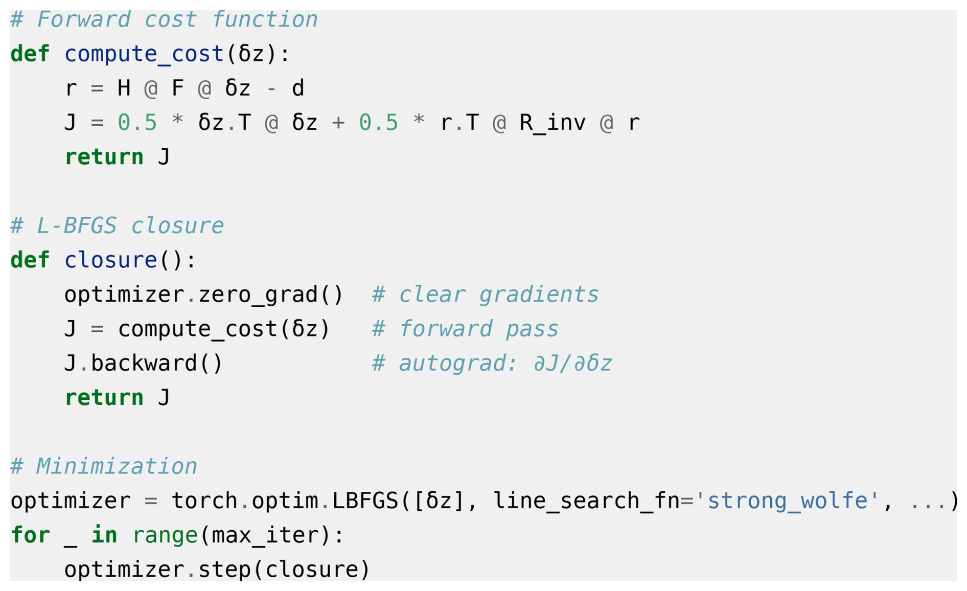
Figure 2 Simplified pseudo-code of the AD-based 3DVar minimization in PY3DVar. R_inv denotes the inverse of the observation error covariance R.

2.6 Background error covariance modeling

The key components of the background error covariance matrix B, namely, the background error standard deviation matrix D, the vertical background error correlation matrix C_z, and the horizontal correlation scale parameter L, are statistically estimated using the National Meteorological Center (NMC) method (Parrish and Derber, 1992). In this procedure, 24 and 48 h forecast experiments are initiated daily at 00:00 UTC for 30 consecutive days. The forecast difference field ϵ is then constructed from forecasts at the same time, calculated as $\mathit{ϵ}=X_{\mathrm{48}\mathrm{h}}-X_{\mathrm{24}\mathrm{h}}$. These forecasts were run with the same model configuration as the assimilation experiments, ensuring consistency between the estimated background error statistics and the assimilation cycles.

The background error standard deviation matrix D is a diagonal matrix. The values for each control variable in D are computed from the standard deviation of the 30 d forecast difference field:

$$\begin{array}{}\text{(5)}& \mathbf{D}=\sqrt{{\displaystyle \frac{\mathrm{1}}{N-\mathrm{1}}}\sum _{i=\mathrm{1}}^N({\mathit{ϵ}}_i-\stackrel{\mathrm{‾}}{\mathit{ϵ}}{)}^{\mathrm{2}}}\end{array}$$

where N is the number of days (N = 30 in this study). The vertical profiles of the background error standard deviation for each control variable are shown in Fig. 3.

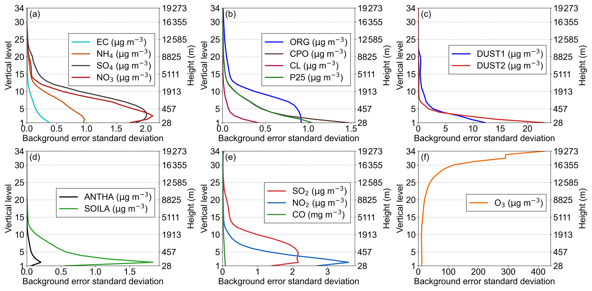
Figure 3 Vertical profiles of background error standard deviation for each control variable: (a) EC, NH₄, SO₄, NO₃; (b) ORG, CPO, CL, P25; (c) DUST1, DUST2; (d) ANTHA, SOILA; (e) SO₂, NO₂, CO; (f) O₃.

The vertical correlation matrix C_z is obtained by calculating the correlation coefficients of the same variable between different model layers. Its matrix elements can be expressed as:

$$\begin{array}{}\text{(6)}& [{\mathbf{C}}_z{]}_{mn}={\displaystyle \frac{\mathrm{cov}(m,n)}{{\mathit{\sigma }}_{{\mathit{ϵ}}_m}\cdot {\mathit{\sigma }}_{{\mathit{ϵ}}_n}}}\end{array}$$

Here, ϵ_m and ϵ_n represent the forecast differences at the mth and nth layers, respectively, cov denotes the covariance, and σ represents the standard deviation. The distribution of the vertical autocorrelation matrix for the background error of each control variable is shown in Fig. 4.

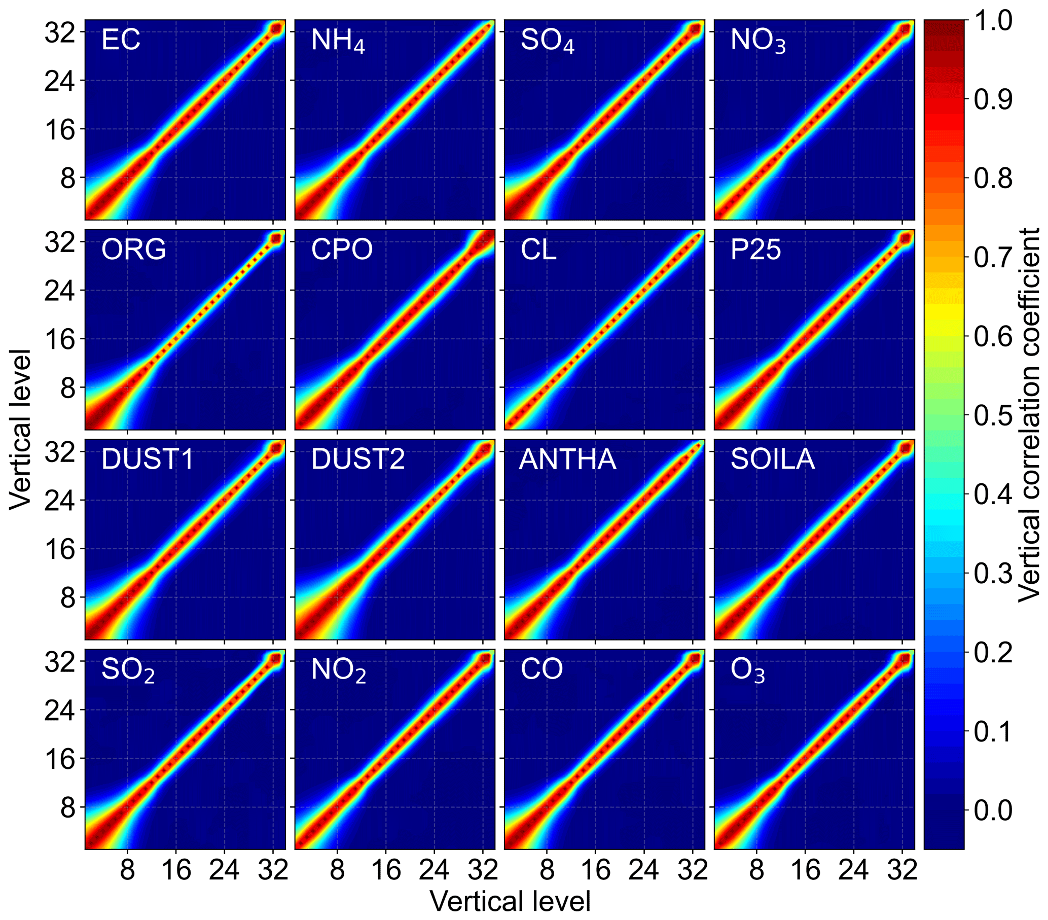
Figure 4 Distribution of the vertical autocorrelation matrix of background error for each control variable.

For the horizontal correlation matrices C_x and C_y, horizontal isotropy is assumed. Consequently, they can be represented by the same decay function, differing only in their dimensions. Their physical meaning is to describe the horizontal correlation between different grid points in the longitudinal or latitudinal direction, specifically fitted using a Gaussian kernel function:

$$\begin{array}{}\text{(7)}& \mathbf{C}(x_{\mathrm{1}},x_{\mathrm{2}})=\exp \left[-{\displaystyle \frac{(x_{\mathrm{1}}-x_{\mathrm{2}}{)}^{\mathrm{2}}}{\mathrm{2}{L}^{\mathrm{2}}}}\right]\end{array}$$

Here, L is the horizontal correlation scale parameter for the background error, x₁ and x₂ represent horizontal grid points.

Horizontal correlation scale parameter L is estimated by analyzing the decay of correlation for the same variable across different horizontal grid distances. The correlation coefficient ρ(d) between all pairs of horizontal grid points is computed as a function of their distance d. L is defined as the maximum grid distance d at which the horizontal correlation coefficient ρ(d) decays to $e^{-\mathrm{1}/\mathrm{2}}$:

$$\begin{array}{}\text{(8)}& L=max\left\{d\right|\mathit{\rho }\left(d\right)⩾e^{-\mathrm{1}/\mathrm{2}}\mathit{\}}\end{array}$$

The horizontal correlation scale parameter L quantitatively describes the decay characteristics of background error correlation between different grid points with increasing distance. Its physical meaning is that when the distance between two horizontal grid points exceeds L, the correlation coefficient between their background errors falls below $e^{-\mathrm{1}/\mathrm{2}}$ (approximately 0.6065), indicating that their statistical correlation has significantly weakened. This parameter quantifies the decay rate of horizontal correlation and is a key parameter for describing the horizontal structure of the background error covariance. The computed values of L are used to construct the horizontal correlation matrices C_x and C_y, which characterize the spatial horizontal correlation structure and directly determine the shape of the Gaussian correlation kernel function. The decay of the horizontal background error correlation coefficient with distance and the corresponding L value for each control variable are shown in Fig. 5.

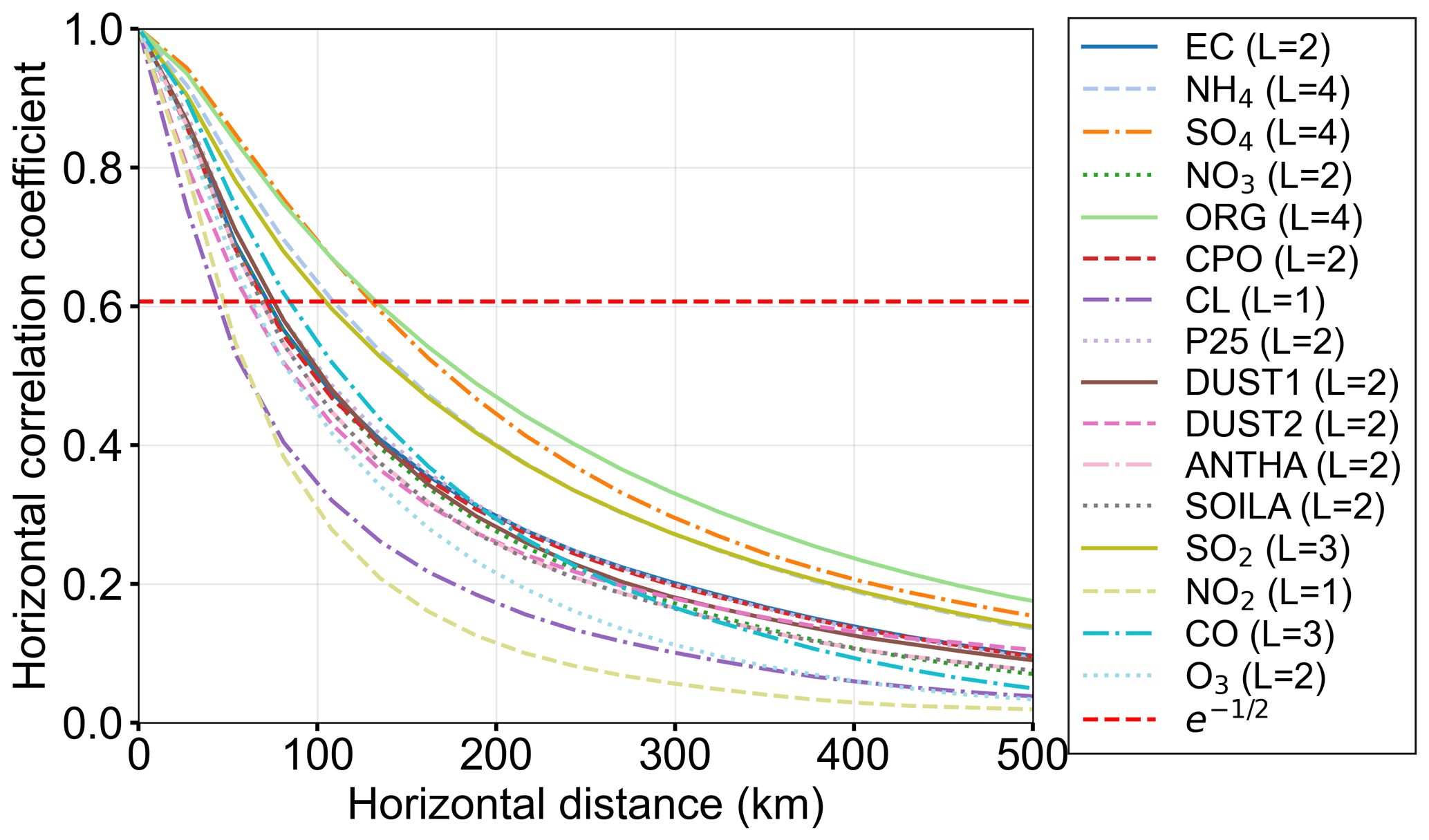
Figure 5 Decay of horizontal background error correlation coefficient with distance for each control variable.

To achieve efficient computation, the three correlation matrices C_x, C_y and C_z are further decomposed via Cholesky decomposition. Each is expressed as the product of a lower triangular matrix and an upper triangular matrix (e.g., ${\mathbf{C}}_x={\mathbf{C}}_{x_{\mathrm{low}}}\cdot {\mathbf{C}}_{x_{\mathrm{up}}}$), where these two triangular matrices are transposes of each other (i.e., ${\mathbf{C}}_{x_{\mathrm{up}}}={\mathbf{C}}_{x_{\mathrm{low}}}^{\mathrm{T}}$, where T denotes transpose). During the actual assimilation process, only the lower triangular matrices for these three directions are retained and used, thereby avoiding direct manipulation of the full B matrix.

Figure 3 shows the vertical profiles of the background error standard deviation, which quantifies the uncertainty of the model background field across different vertical layers and for different variables. In the 3DVar assimilation process, the D matrix assigns the relative weights of the analysis increments among the control variables in response to observational information. A larger background error standard deviation for a variable indicates higher uncertainty in the background field simulation, allowing for greater adjustment by observational information during assimilation. Conversely, a smaller standard deviation implies higher confidence in the background field, resulting in more moderate increments. Figure 3 reveals significant differences in the near-surface values among the variables. The background error standard deviations for DUST1 and DUST2 are the largest, substantially higher than those of other variables. With increasing height, the background error standard deviations for most variables generally exhibit a decaying trend, and the differences between them gradually diminish. In contrast, O₃ exhibits an increasing trend with height, reflecting the enhanced background uncertainty associated with its photochemical production and longer lifetime in the upper troposphere. In terms of profile shape and decay rate, DUST1 and DUST2 decay most rapidly, while the decay of the other variables is relatively gradual. Additionally, some species show non-monotonic vertical variations, such as a near-surface peak for SO₂ and NO₂, indicating distinct vertical uncertainty characteristics for these species.

Figure 4 presents the vertical autocorrelation matrices of the background error for each control variable. These matrices govern how surface observational information propagates across vertical levels during assimilation. Although the detailed structures differ among variables, all matrices exhibit strong correlations in the near-surface layers that weaken with increasing height. This indicates that surface observations primarily constrain the lower levels of the model, while their influence on the upper levels is more limited.

Figure 5 presents the decay curves of the horizontal background error correlation coefficient with grid distance for each control variable, along with their corresponding horizontal correlation scale parameter L. These curves are derived directly from the empirical correlation statistics computed over the 30 d forecast difference fields, rather than from a mathematical fitting process. This correlation coefficient determines the horizontal spread and weight allocation of observational information. The horizontal axis represents physical distance, calculated from a model grid spacing of approximately 27 km. To focus on the region of physical significance, the figure only displays distances up to 500 km, as correlation coefficients beyond this range are already negligible. These empirical curves exhibit an initially rapid then gradually slowing decay with distance, consistent with the Gaussian-type correlation model. The decay rates differ considerably among the variables, yielding L values that range from 1 to 4 grid units. This spread reflects the heterogeneity in the horizontal spatial correlation of background errors for different pollutants.

3 Experimental design and evaluation metrics

3.1 Experimental design

To systematically evaluate the performance and effectiveness of the PY3DVar assimilation system, this study designed three categories of numerical experiments: idealized experiment, 20 d real-case assimilation and forecast experiments, and multi-core CPU parallel performance benchmark tests.

3.1.1 Computing platforms

The CPU platform is a single node equipped with two AMD EPYC 7542 processors (32 physical cores per processor, 64 cores in total @ 2.9 GHz) and 256 GB of system memory. The GPU platform employs an NVIDIA RTX 3090 with 24 GB of device memory. The FT3DVar system runs exclusively on CPU, whereas PY3DVar is deployed on both CPU and GPU platforms. All calculations adopted 32-bit floating-point precision.

3.1.2 Idealized experiment

An idealized twin-observation experiment was designed based on the 27 km grid. Its purpose is to test the system's capability to generate physically reasonable increment fields with observations of varying magnitudes. Two observation sites were positioned far apart to avoid spatial correlation interference, ensuring the independence of constraints from different observation magnitudes. For the low-concentration observation site (37.2104° N, 116.0108° E), the prescribed concentrations were 0.01 µg m⁻³ (SO₂, NO₂, O₃), 0.01 mg m⁻³ (CO), 1.00 µg m⁻³ (PM_2.5) and 1.50 µg m⁻³ (PM₁₀). For the high-concentration site (37.8666° N, 92.3785° E), the corresponding values were 200 µg m⁻³ (SO₂, NO₂, O₃), 10 mg m⁻³ (CO), 500 µg m⁻³ (PM_2.5) and 700 µg m⁻³ (PM₁₀). By comparing the analysis field with the background field, the ability of the assimilation system to produce physically sound increment fields under different concentration magnitudes can be verified.

3.1.3 Real-case assimilation and forecast experiments

Twenty consecutive assimilation cycles were conducted at 00:00 UTC each day from 10–29 October 2023. For each cycle, the assimilation was performed using two systems: (1) FT3DVar on the CPU platform with 64 cores, and (2) PY3DVar on the GPU platform. Following each assimilation, a 24 h forecast was launched from the respective analysis field. A control forecast was also initiated from the original, unassimilated background field (labeled Control). All three forecasts for each cycle shared identical model configurations except for the initial conditions.

3.1.4 Multi-core CPU parallel benchmark tests

To evaluate the parallel scalability of both FT3DVar and PY3DVar on CPU platforms, the 20 assimilation cases were repeated using 1, 2, 4, 8, 16, 32, and 64 CPU cores. Only the assimilation step was performed in these tests, without the subsequent 24 h forecast. This experiment enables a direct comparison of how the computational efficiency of each system scales with increasing parallel resources.

3.2 Evaluation metrics

To quantitatively evaluate the assimilation and forecasting performance of both PY3DVar and FT3DVar, this study employs three statistical metrics: the correlation coefficient (CORR), root mean square error (RMSE), and mean absolute error (MAE). CORR measures the linear correlation between simulated and observed values; RMSE is more sensitive to extreme errors and reflects the overall deviation of the simulation results; MAE measures the average absolute error between simulated and observed values and is less sensitive to outliers. The formulas for each metric are as follows:

$$\begin{array}{}\text{(9)}& {\displaystyle }\mathrm{CORR}={\displaystyle \frac{\sum _{i=\mathrm{1}}^N(M_i-\stackrel{\mathrm{‾}}{M})(O_i-\stackrel{\mathrm{‾}}{O})}{\sqrt{\sum _{i=\mathrm{1}}^N(M_i-\stackrel{\mathrm{‾}}{M}{)}^{\mathrm{2}}\sum _{i=\mathrm{1}}^N(O_i-\stackrel{\mathrm{‾}}{O}{)}^{\mathrm{2}}}}}\text{(10)}& {\displaystyle }\mathrm{RMSE}=\sqrt{{\displaystyle \frac{\mathrm{1}}{N}}\sum _{i=\mathrm{1}}^N(M_i-O_i{)}^{\mathrm{2}}}\text{(11)}& {\displaystyle }\mathrm{MAE}={\displaystyle \frac{\mathrm{1}}{N}}\sum _{i=\mathrm{1}}^N|M_i-O_i|\end{array}$$

where M_i and O_i represent the simulated value and observed value for the ith sample, respectively. $\stackrel{\mathrm{‾}}{M}$ and $\stackrel{\mathrm{‾}}{O}$ are the average values of the simulated and observed values, respectively. N is the total number of samples.

4 Results and evaluation

4.1 Evaluation of the idealized experiment

Figures 6 and 7 present the surface increment fields generated by PY3DVar and FT3DVar in the idealized experiment, while Figs. 8 and 9 show the corresponding vertical cross-sections. The PM_2.5 and PM₁₀ increments are diagnosed as the sum of the relevant aerosol control variable increments, while the gaseous pollutant increments are those of the corresponding control variables.

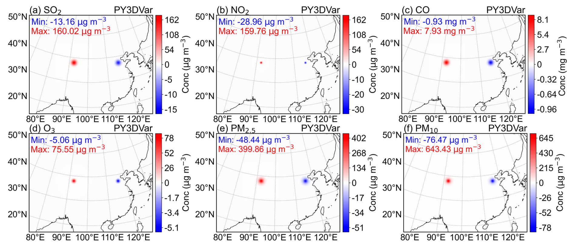
Figure 6 Surface increment fields for the six pollutants (a – SO₂, b – NO₂, c – CO, d – O₃, e – PM_2.5, f – PM₁₀) from the PY3DVar assimilation system in the idealized experiment. Blue and red colors represent negative and positive increments, respectively.

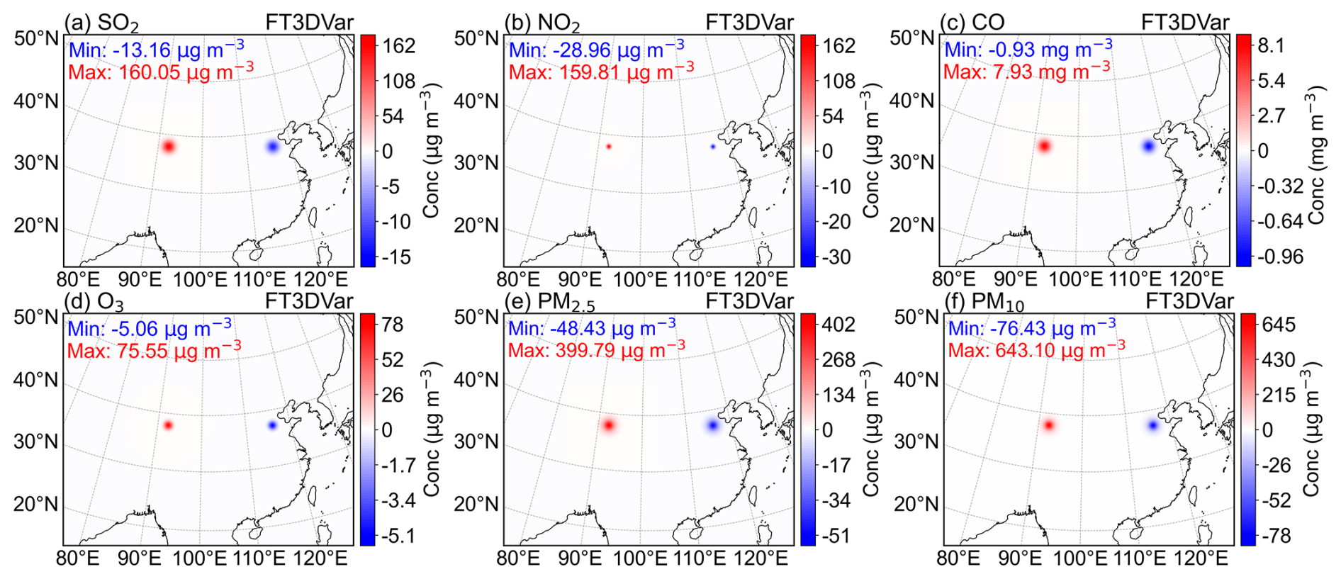
Figure 7 Surface increment fields for the six pollutants (a – SO₂, b – NO₂, c – CO, d – O₃, e – PM_2.5, f – PM₁₀) from the FT3DVar assimilation system in the idealized experiment. Blue and red colors represent negative and positive increments, respectively.

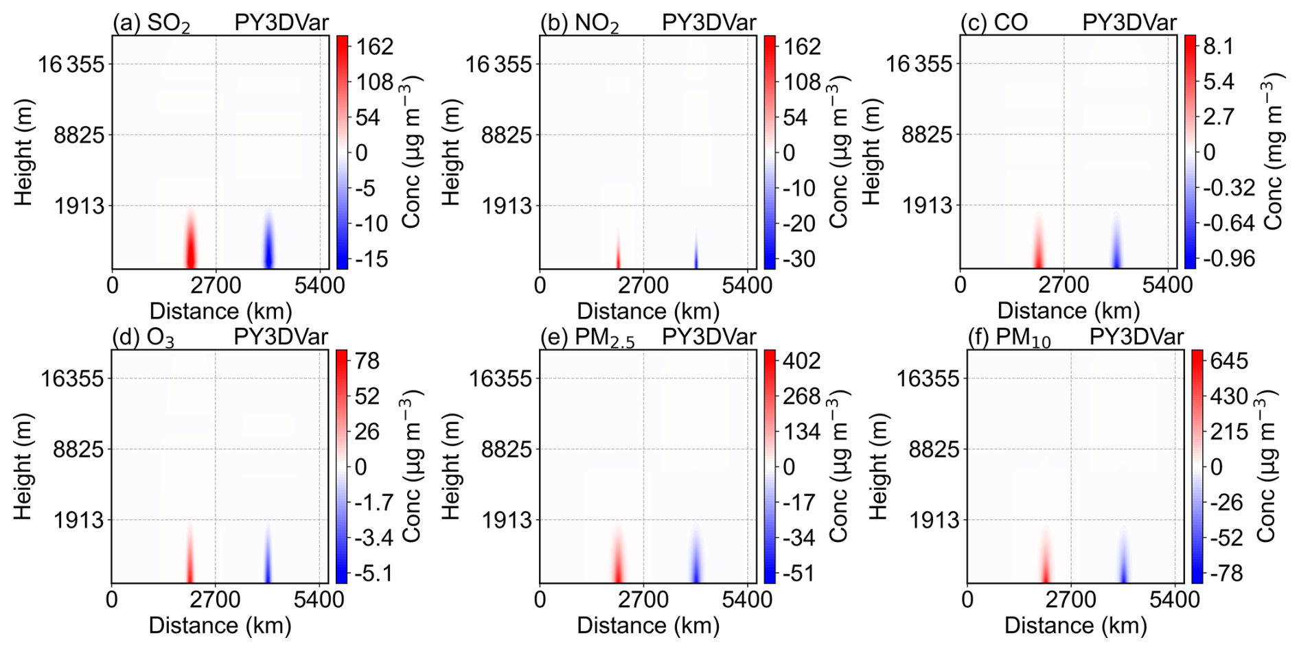
Figure 8 Vertical cross-sections of the increment fields for the six pollutants (a – SO₂, b – NO₂, c – CO, d – O₃, e – PM_2.5, f – PM₁₀) from the PY3DVar assimilation system in the idealized experiment. Blue and red colors represent negative and positive increments, respectively.

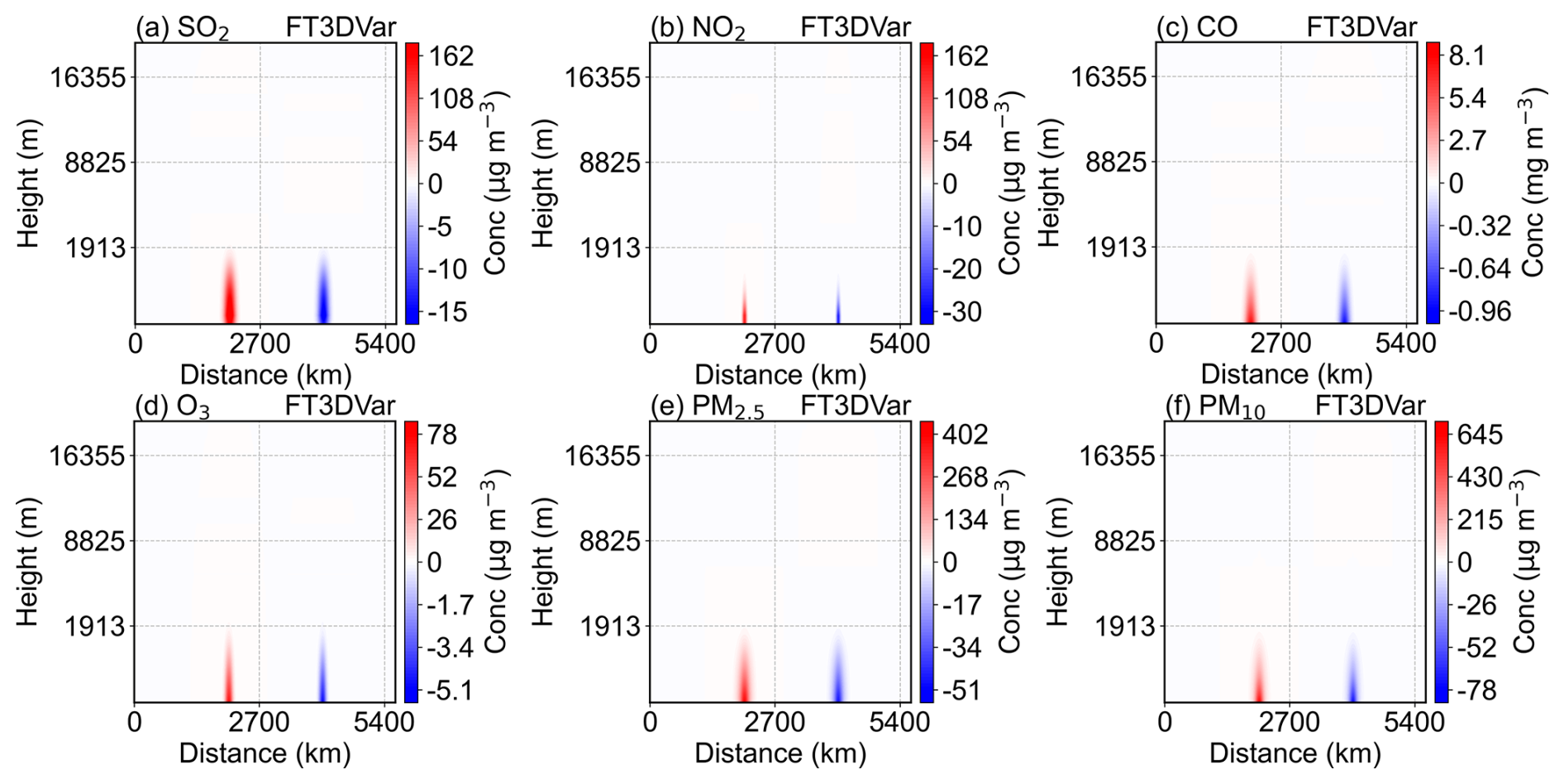
Figure 9 Vertical cross-sections of the increment fields for the six pollutants (a – SO₂, b – NO₂, c – CO, d – O₃, e – PM_2.5, f – PM₁₀) from the FT3DVar assimilation system in the idealized experiment. Blue and red colors represent negative and positive increments, respectively.

For both systems, the increments exhibit Gaussian-type horizontal distributions centered on the observation points, decaying with distance, and columnar vertical structures that weaken with height. The vertical extent of the increments is controlled by the vertical correlation matrix C_z, while their horizontal spread is governed by the horizontal correlation scale parameter L, consistent with the background error characteristics described in Sect. 2.6. Differences in L and C_z among pollutants account for the observed variations in horizontal spread and vertical column thickness.

Figure 10 further compares the analysis fields under high and low concentration conditions, showing that both systems effectively correct the background field toward the observations, with negligible differences between their analysis values. Together, Figs. 6–10 demonstrate that PY3DVar and FT3DVar produce highly consistent increment fields and analysis values under idealized conditions, confirming that PY3DVar achieves numerical accuracy and physical consistency comparable to FT3DVar.

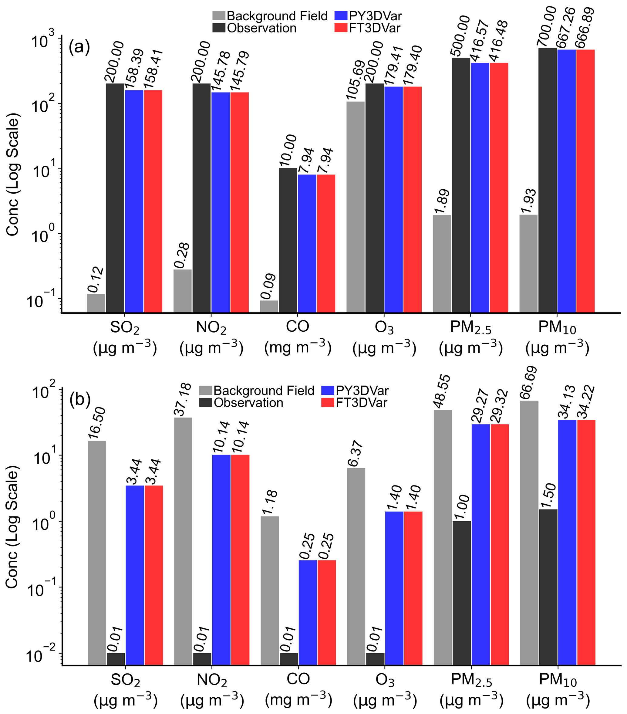
Figure 10 Comparison of background field (gray), observation (black), FT3DVar analysis field (red), and PY3DVar analysis field (blue) under extremely high (a) and low (b) concentration conditions.

4.2 Evaluation of the analysis fields

Figures 11 and 12 present scatter plots comparing simulated and observed concentrations across the 20 d period for the Control run, the PY3DVar assimilation experiment, and the FT3DVar assimilation experiment, respectively. In these figures, blue dots represent the control experiment, while red dots represent the assimilation experiments. PY3DVar was run on the GPU platform, while FT3DVar was run on the CPU platform with 64 cores. Regarding the distribution pattern, the blue dots from the Control experiment are relatively scattered and deviate considerably from the 1 : 1 line. In contrast, the red dots from the assimilation experiments show a clear convergence towards the 1 : 1 line, indicating that both assimilation systems effectively improve the quality of the initial field, with a very pronounced improvement effect.

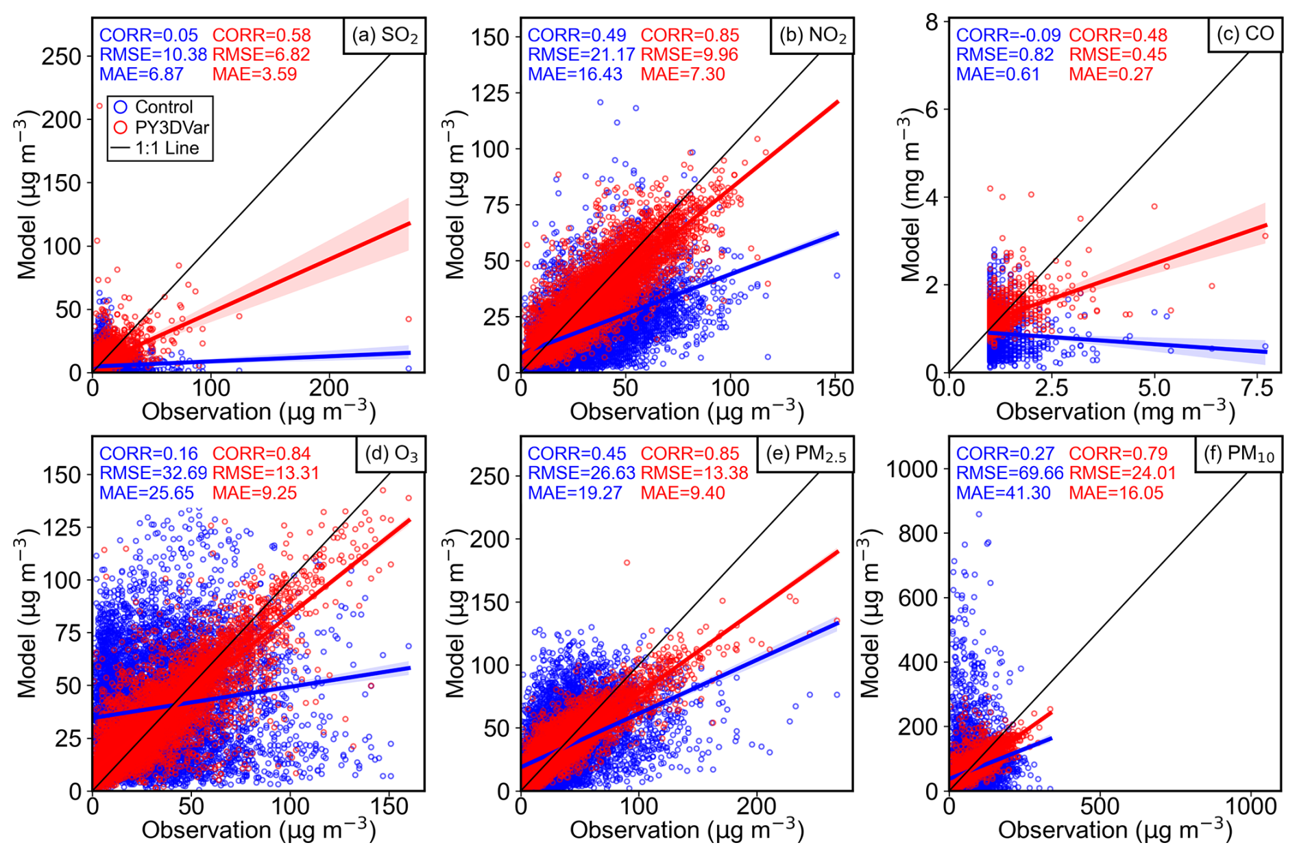
Figure 11 Scatter plots of observations against Control (blue) and PY3DVar analysis (red) concentrations. The black line is the 1 : 1 line.

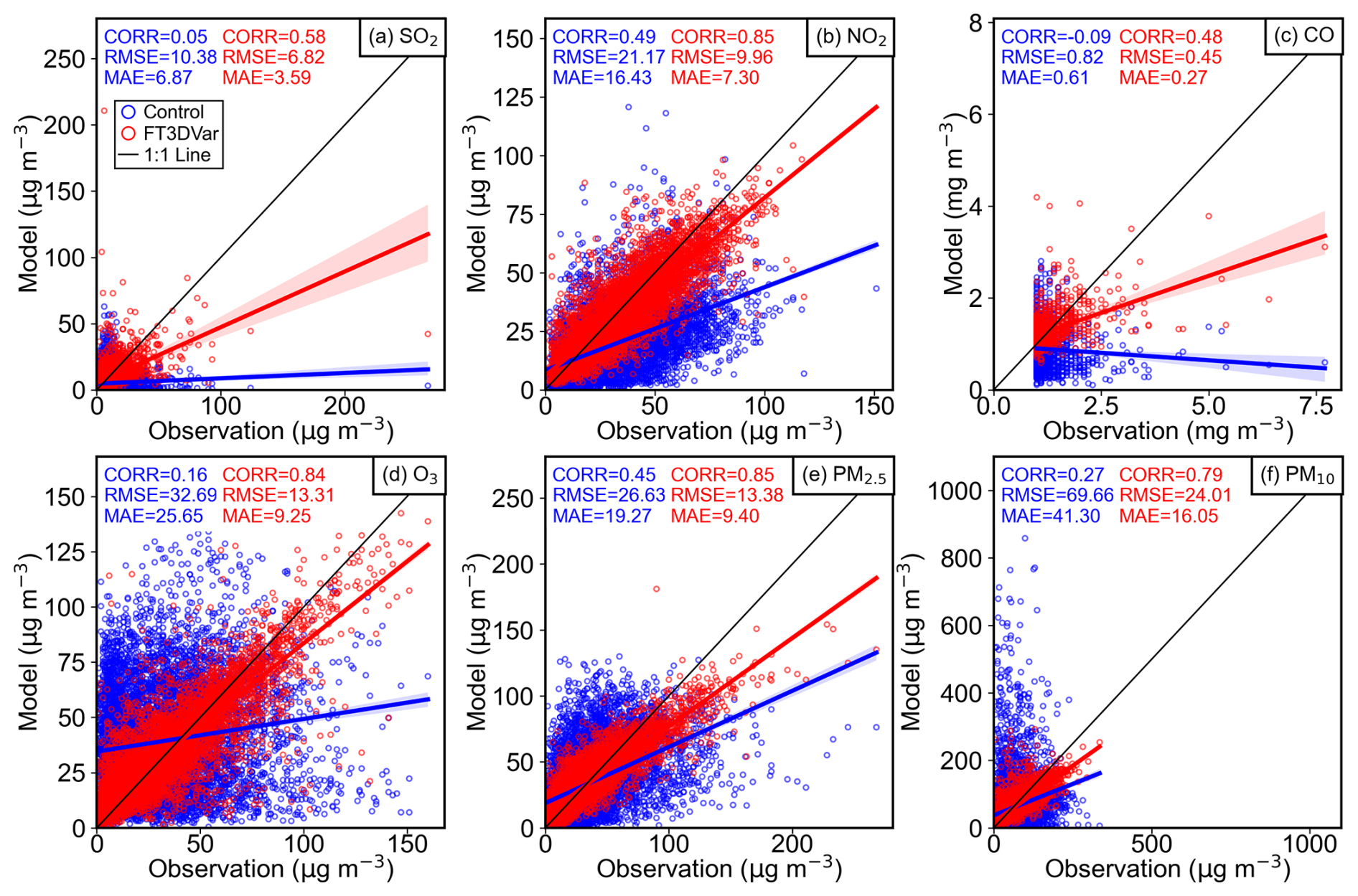
Figure 12 Scatter plots of observations against Control (blue) and FT3DVar analysis (red) concentrations. The black line is the 1 : 1 line.

Examining the specific evaluation metrics, the degree of improvement in the initial fields varies among different pollutants. After assimilation, the CORR values for all pollutants increased significantly. The CORR reached 0.58 for SO₂ and 0.48 for CO, those for NO₂, O₃ and PM_2.5 were above 0.8, and the CORR for PM₁₀ was 0.79. Concurrently, the RMSE and MAE for all pollutants decreased substantially compared to the Control experiment, further confirming the corrective effect of assimilation on initial field biases. The scatter distributions from PY3DVar and FT3DVar are nearly identical across all pollutants, and the corresponding CORR, RMSE, and MAE values are essentially identical. This strong quantitative agreement, consistent with the findings of the idealized experiment, confirms that the two systems achieve equivalent assimilation performance in real-case applications.

4.3 Iteration behavior and computational efficiency

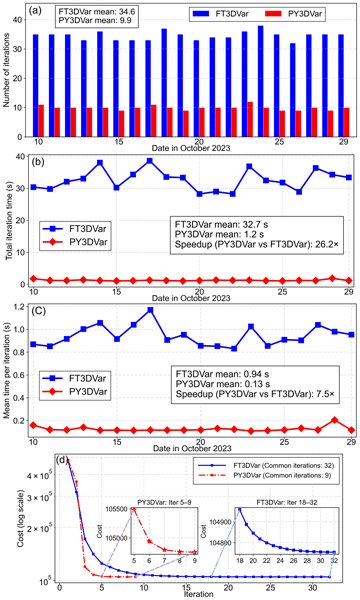
This section comprehensively evaluates the iteration behavior and computational efficiency of the conventional FT3DVar and the developed PY3DVar (GPU-based implementation) using 20 consecutive days of real atmospheric assimilation experiments. The analysis encompasses iteration counts, total and per-iteration time consumption, and cost function convergence characteristics, as presented in Fig. 13. Figure 13a illustrates the number of iterations required per assimilation cycle throughout the 20 d experiment. FT3DVar requires an average of 34.6 iterations to converge, whereas PY3DVar converges in only 9.9 iterations on average. As discussed in Sect. 2.5, both systems adopt identical L-BFGS parameter settings and the same convergence criterion; the primary difference lies in their internal line search algorithms – the Moré-Thuente scheme for FT3DVar versus the Strong Wolfe scheme for PY3DVar. The Strong Wolfe line search generally yields a larger per-iteration reduction in the cost function, which partly explains the substantially fewer iterations required by PY3DVar to achieve convergence. Figure 13b presents the total iteration time per cycle. On average, FT3DVar requires 32.7 s per cycle, while PY3DVar requires only 1.2 s, yielding a 26.2 × speedup over the traditional system. The per-iteration time shown in Fig. 13c further elucidates the source of this performance discrepancy. The mean per-iteration time is 0.94 s for FT3DVar and 0.13 s for PY3DVar, corresponding to a 7.5 × speedup. Combined with the significantly reduced iteration count (Fig. 13a), these two factors collectively account for the high overall efficiency of PY3DVar. The GPU-accelerated execution of vectorized tensor operations, which is central to the PyTorch framework, is the primary contributor to the drastic per-iteration time reduction. Figure 13d displays the mean descent curves of the cost function within the common iteration range. All curves exhibit a typical nonlinear convergence pattern, characterized by a rapid initial drop followed by a gradually slowing decline, eventually leveling off as the systems approach the optimal solution. Consistent with the fewer iterations depicted in Fig. 13a, PY3DVar reduces the cost function much more aggressively in the early iterations than FT3DVar. Specifically, the descent curve of FT3DVar becomes notably flat and decreases only very slowly after the 10th iteration. The close agreement between the final cost values of PY3DVar and FT3DVar further confirms that both systems achieve highly consistent assimilation accuracy.

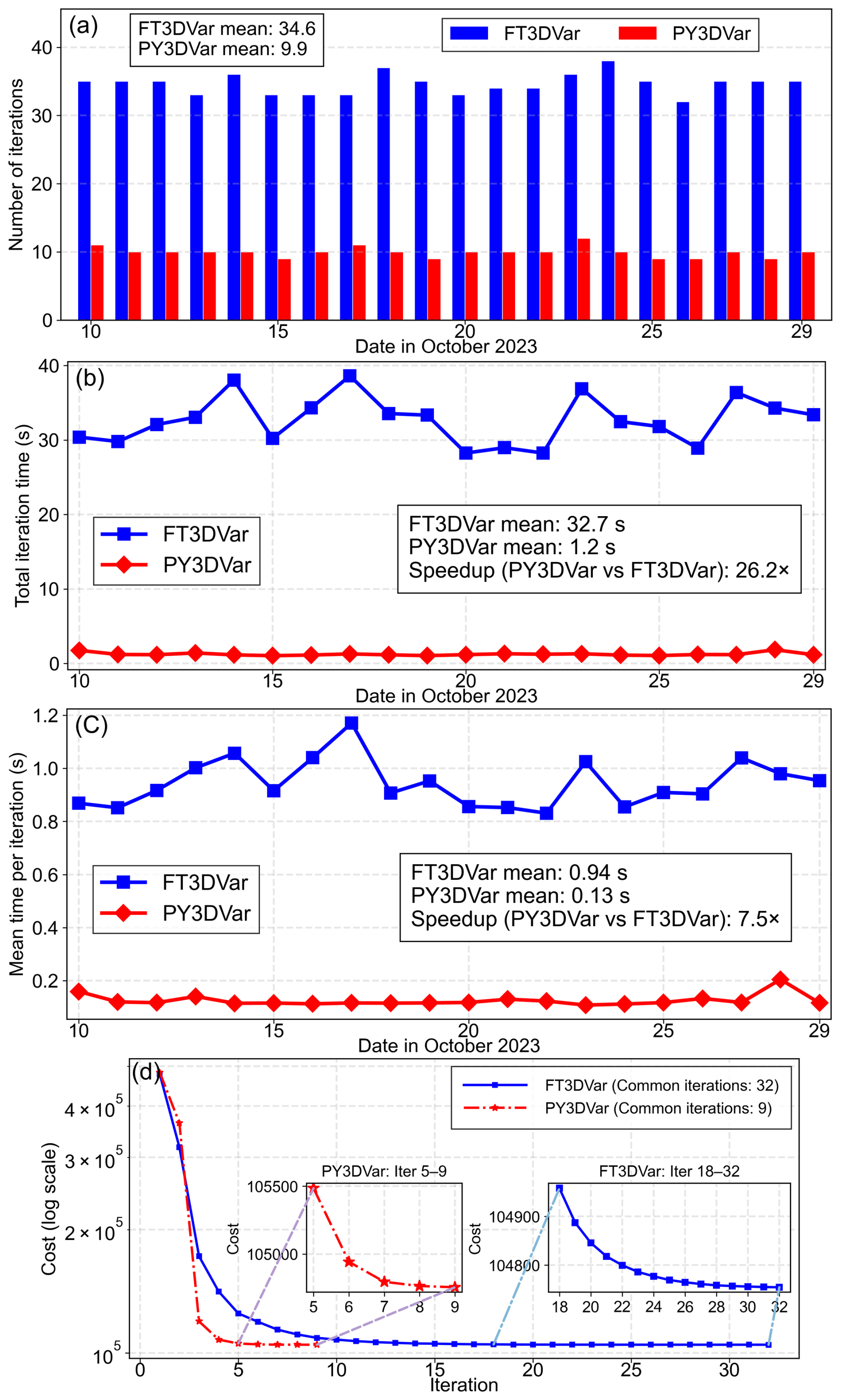
Figure 13 Statistical characteristics of iteration performance for different assimilation systems. (a) Number of iterations; (b) Total iteration time; (c) Mean time per iteration; (d) Mean descent curves of cost function within common iteration steps. Blue and red bars/lines represent FT3DVar and PY3DVar, respectively.

4.4 Evaluation of multi-core CPU scalability

Figure 14 illustrates the parallel scalability and computational efficiency of FT3DVar and PY3DVar across different CPU core configurations (1, 2, 4, 8, 16, 32, and 64 cores), based on averaged results from a 20 d continuous assimilation experiment.

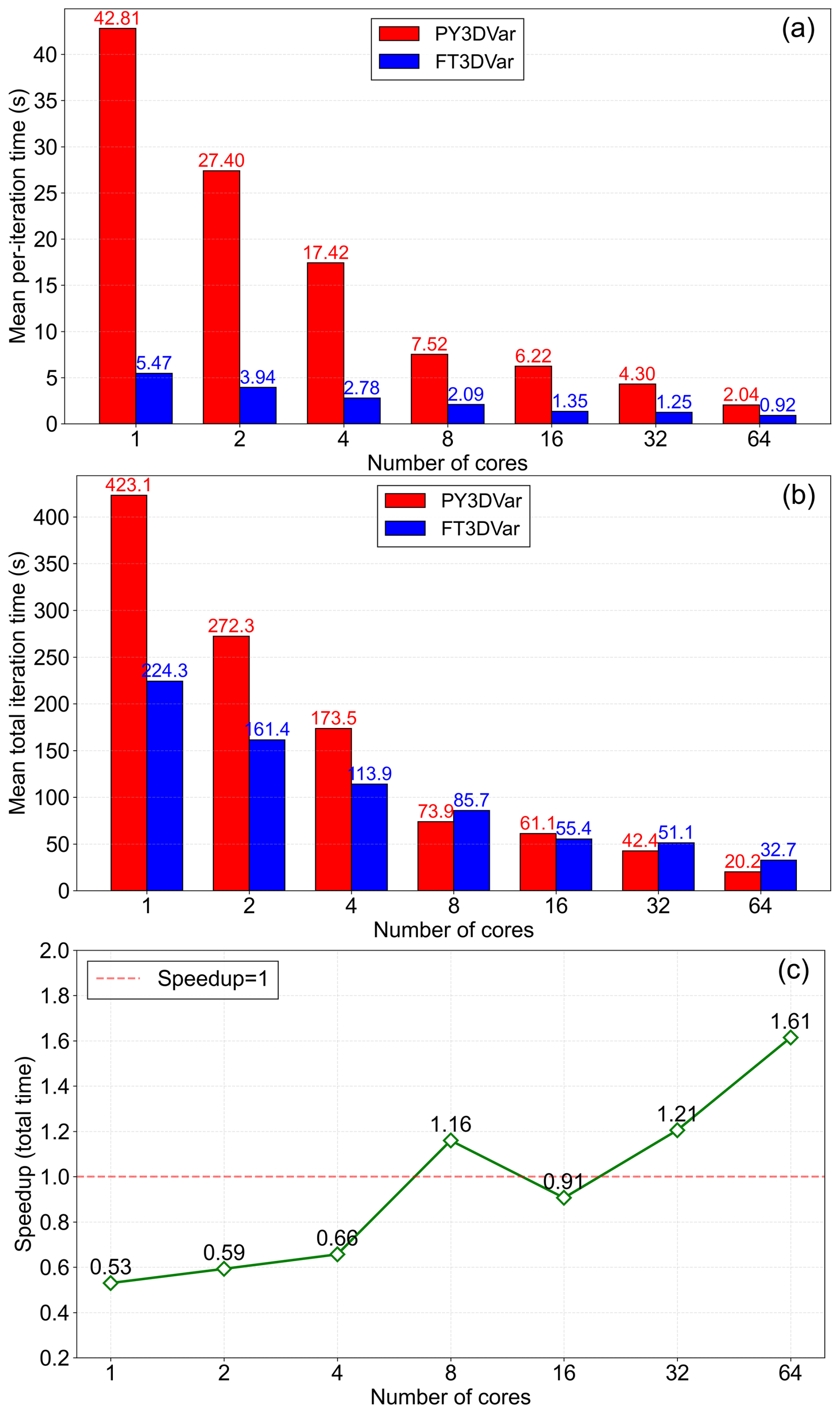
Figure 14 Parallel scalability of FT3DVar (blue) and PY3DVar (red) across CPU core counts. (a) Mean per-iteration time. (b) Mean total iteration time. (c) Speedup of PY3DVar relative to FT3DVar. Dashed line in (c): speedup = 1.

In terms of per-iteration time, FT3DVar outperforms PY3DVar across all tested core counts, decreasing from 5.47 to 0.92 s, which reflects the inherent speed of the compiled Fortran implementation. PY3DVar drops more steeply, from 42.81 to 2.04 s, yet remains consistently slower than FT3DVar at every core configuration. The modest absolute reduction in FT3DVar's per-iteration time is due to its already fast single-core baseline, which leaves limited room for further improvement.

Regarding total iteration time, both systems benefit substantially from increasing parallelism. FT3DVar declines steadily from 224.3 s at a single core to 32.7 s at 64 cores. PY3DVar starts from a much higher baseline of 423.1 s but exhibits a steeper reduction, reaching 20.2 s at 64 cores. Despite its per-iteration disadvantage, PY3DVar achieves a shorter total assimilation time than FT3DVar at 8 cores (73.9 s vs. 85.7 s), 32 cores (42.4 s vs. 51.1 s) and 64 cores (20.2 s vs. 32.7 s). This reversal results from the combined effect of PY3DVar's substantially fewer iterations (9.9 vs. 34.6; Fig. 13a) and its stronger parallel scaling at higher core counts. At 1, 2, 4, and 16 cores, FT3DVar retains the total-time advantage, as its faster per-iteration speed outweighs the difference in iteration count. The speedup of PY3DVar relative to FT3DVar (Fig. 14c) exceeds unity at 8, 32, and 64 cores, and reaches 1.61 at 64 cores.

In summary, FT3DVar benefits from inherently faster single-core performance, while PY3DVar compensates through stronger parallel scalability and far fewer iterations. These two factors together enable PY3DVar to surpass FT3DVar in total assimilation time at 8, 32, and 64 cores.

4.5 Evaluation of 24 h forecast performance

Figures 15 and 16 display the 20 d averaged temporal evolution of the CORR, RMSE, and MAE for various pollutants during the 24 h forecast period, initialized from the analysis fields of PY3DVar and FT3DVar, respectively. Comparing the forecast performance of the two systems reveals that the curves of the forecast metrics for all pollutants are fundamentally consistent in terms of morphological characteristics, temporal trends, and numerical values. This finding corroborates the previous results showing minor differences in idealized experiment increment fields, similar analysis field effectiveness in the real case, and comparable cost function convergence characteristics during iteration. It fully demonstrates that the PY3DVar system achieves performance consistent with the mature FT3DVar system not only in initial field assimilation but also in subsequent forecast applications, thoroughly verifying the reliability and practical utility of its assimilation results.

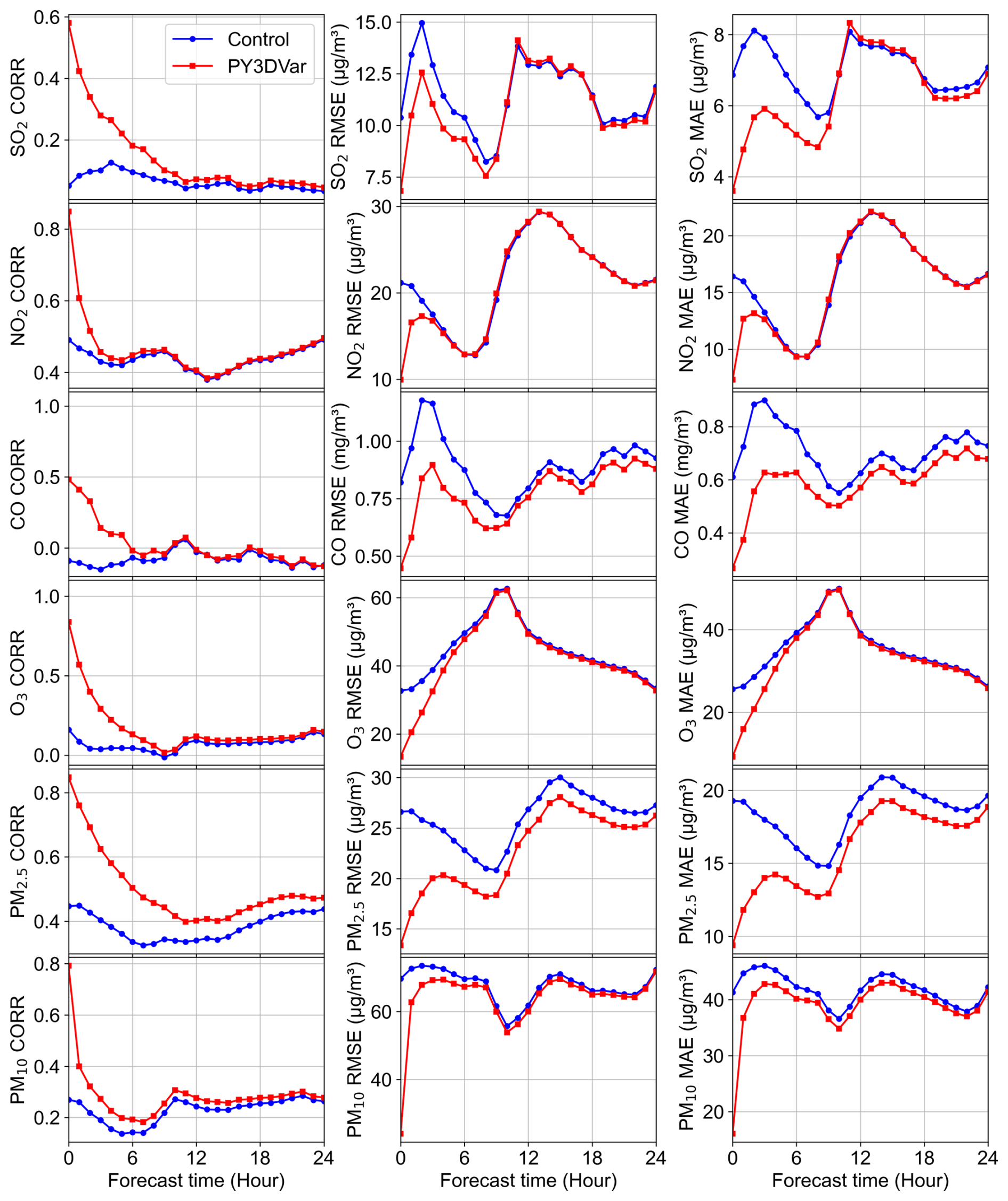
Figure 15 Temporal evolution of forecast performance for PY3DVar (red) and Control (blue) over the 24 h period. From left to right: CORR, RMSE, MAE. From top to bottom: SO₂, NO₂, CO, O₃, PM_2.5, PM₁₀.

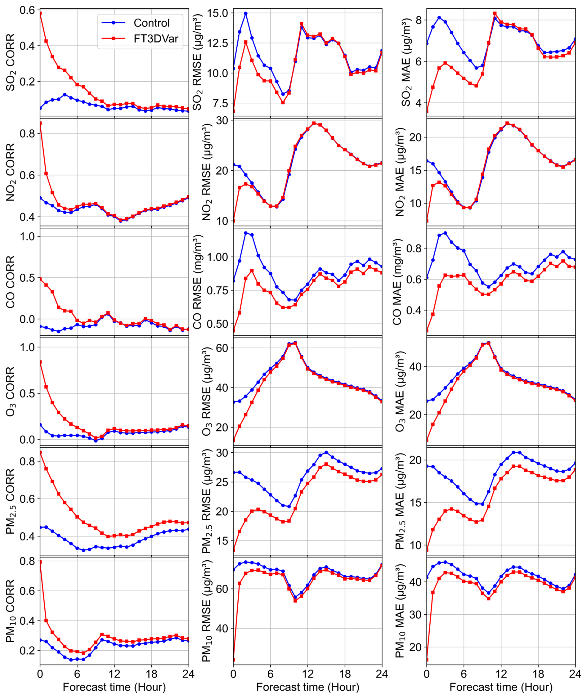
Figure 16 Temporal evolution of forecast performance for FT3DVar (red) and Control (blue) over the 24 h period. From left to right: CORR, RMSE, MAE. From top to bottom: SO₂, NO₂, CO, O₃, PM_2.5, PM₁₀.

Regarding the evolution of forecast performance, although the initial field is significantly optimized by assimilation, this positive effect decays rapidly as the forecast lead time increases (Pagowski et al., 2010; Jiang et al., 2013; Li et al., 2013). This decay primarily stems from inherent model uncertainties, spatiotemporal errors in emission inventories, and inaccuracies in the simulated meteorological fields affecting pollutant dispersion and transport. These errors accumulate during the forecast process and gradually become dominant, thereby progressively diminishing the positive effect of the assimilation improvements.

It is noteworthy that the duration of the positive assimilation effect varies significantly among different pollutants. The improvement for SO₂, CO, PM_2.5, and PM₁₀ can be maintained for over 24 h, whereas the positive effects for NO₂ and O₃ are shorter, lasting approximately 6 and 8 h, respectively. This difference is mainly determined by the respective physicochemical properties and dominant life-cycle processes of the pollutants. SO₂, CO, and particulate matter typically have longer atmospheric lifetimes, and their concentration distributions are more influenced by large-scale transport processes. Consequently, improvements in the initial field yield more lasting positive effects. In contrast, NO₂ and O₃ have strong photochemical reactivity. Their concentrations during daytime are more significantly governed by local photochemical processes and boundary layer variations, causing the initial field improvements from assimilation to dissipate quickly.

In summary, PY3DVar achieves assimilation accuracy comparable to FT3DVar and delivers sustained forecast improvements. Although these improvements decay with forecast time, the benefits for short-term forecasts are evident, particularly for longer-lived species such as SO₂, CO, and particulate matter.

5 Summary

Based on the 3DVar assimilation principle and integrated with the PyTorch DL framework, this study successfully developed a GPU-accelerated atmospheric chemical 3DVar assimilation system (PY3DVar). The system is built upon the CMAQ-AERO5 aerosol scheme coupled with the WRF-Chem model. It consolidates 27 aerosol species into 12 control variables and directly designates four gaseous pollutants as additional control variables. The background error covariance matrix is constructed using the NMC method, enabling the simultaneous assimilation of surface concentrations of SO₂, NO₂, CO, O₃, PM_2.5, and PM₁₀. At the algorithm level, the core computations replace traditional Fortran loops with PyTorch tensor operations. Leveraging the AD mechanism greatly simplifies the gradient derivation required for the minimization, and the PyTorch built-in L-BFGS optimizer, along with the tensorized computation, facilitates efficient minimization on both CPU and GPU hardware.

To comprehensively evaluate the system, this study conducted a series of experiments: an idealized test to verify physical correctness, 20 d real-case assimilation cycles using both FT3DVar and PY3DVar (GPU-accelerated), and parallel scalability assessments across 1, 2, 4, 8, 16, 32, and 64 CPU cores. The system's performance was benchmarked against the traditional FT3DVar in terms of assimilation accuracy, computational efficiency, and forecast skill. The idealized experiments demonstrate that PY3DVar propagates observation information through the background error covariance to generate Gaussian-distributed increment fields. These fields exhibit high consistency with those produced by FT3DVar, confirming the physical soundness and numerical correctness of the new framework. In the 20 d real-case assimilation experiments, PY3DVar substantially improved the model background field across all six target pollutants. Compared to the control run, the assimilation significantly enhanced the CORR between the analysis and observations, while notably reducing the RMSE and MAE. Furthermore, the final analysis fields produced by PY3DVar were nearly identical to those of FT3DVar. This agreement verifies that the GPU-based implementation achieves the same high assimilation accuracy as the traditional Fortran system. In terms of computational efficiency, PY3DVar demonstrates a clear advantage, which is most pronounced on GPU hardware. With FT3DVar on 64 CPU cores requiring an average of 32.7 s per assimilation cycle, the GPU-accelerated PY3DVar completes the same task in 1.2 s, a 26.2-fold speedup. The mean iteration count is correspondingly reduced from 34.6 (FT3DVar) to 9.9 (PY3DVar). This speedup results from two factors: the massive parallelism of tensor operations on the GPU, and the faster convergence of the PyTorch L-BFGS optimizer, whose Strong Wolfe line search yields a larger per-iteration reduction in the cost function than the Moré-Thuente scheme used in FT3DVar. On CPU platforms, although PY3DVar remains slower per iteration than FT3DVar across all tested core counts, its substantially fewer iterations and stronger parallel scaling enable it to surpass FT3DVar in total iteration time at 8, 32, and 64 cores. Overall, PY3DVar's computational efficiency arises from the combination of hardware acceleration and an algorithmic advantage in convergence speed, ensuring competitive performance across diverse computing environments. Finally, short-term forecast experiments demonstrate that the positive impacts of assimilation persist over time. The improvements for SO₂, CO, PM_2.5, and PM₁₀ last for more than 24 h, while those for NO₂ and O₃ maintain significance for over 6 h. Importantly, the decay trends of these forecast improvements are consistent between the PY3DVar and FT3DVar, further validating the robustness and stability of the proposed system across different hardware architectures.

In summary, the PY3DVar system developed in this study achieves substantial improvements in computational efficiency compared to the traditional Fortran-based FT3DVar, while maintaining equivalent assimilation accuracy. This is accomplished through GPU-accelerated tensor computation and the faster convergence of the PyTorch L-BFGS optimizer. Additionally, the use of AD significantly simplifies code development by eliminating the need for manual adjoint coding. The results demonstrate that PY3DVar offers an efficient and practical solution for operational atmospheric chemical data assimilation.