Calibration guidelines and a runoff-isotope module for lake proxy system modeling (PRYSM v2.0)

Lake sediments preserve information about past air temperature and precipitation, providing critical, real-world targets to validate climate models. However, these paleoclimate data encode information about multiple climate signals as well as lake dynamics, which makes comparison of paleoclimate data and model output challenging. Proxy system models (PSMs), or forward models that translate climate variables into proxy units, are tools for mechanistically interpreting paleoclimate data. PRYSM v2.0 is a PSM for paleoclimate data archived in lake sediments. Foundational to the accuracy of the PSM is a comprehensive understanding of the modern lake system supported by observations and meteorological inputs. However, two obstacles exist. First, stable oxygen and hydrogen isotope values in lake water are the target of many proxies preserved in lake sediments, but the PSM does not have a built-in catchment model to aid simulation of isotope values. Additionally, calibration of uncertain model parameters requires observations and expert knowledge of the lake system, yet most sites are unmonitored. Here, we advance PSMs for lake sediment archives by integrating a simple runoff-isotope module that can be adapted to any lake and reproduce the seasonal timing and magnitude of two mid-latitude lakes with contrasting morphometry, hydrology, and mixing regimes. Using multi-year observational datasets from the lakes, we conduct model experiments that require the PSM to predict the temperature and δ²H values of lake water when calibrated to a single observed profile, which mimics common observation collection challenges. For these lakes, observations from the warm, ice-free season are most informative and constrain uncertain parameter values that best generalize to unseen data from other water depths and years. Our framework for running and calibrating the PSM is available as open-source tools in Python, aiding the application of this PSM to the vast global database of lake sediment paleoclimate time series.

1 Introduction

Sediments accumulate over time in the bottom of lakes and preserve information about past air temperature and precipitation over thousands of years. These paleoclimate data can capture times in Earth's history when climate rapidly warmed, providing critical, real-world targets to validate climate models (Braconnot et al., 2012). In fact, time series generated from lake sediments currently comprise ∼25 % of paleoclimate databases (NOAA/World Data Service for Paleoclimatology & Neotoma, 2025). However, lake sediments preserve indirect observations of climate variables made from measurements of physical, biological, and geochemical indicators. These paleoclimate “proxies” are often sensitive to multiple climate variables and additionally to lake dynamics (Castañeda and Schouten, 2011). Therefore, interpreting variables useful for climate model validation (e.g. rainfall amount, air temperature) from lake sediments can be challenging.

The development of PRYSM v2.0, a proxy system model (PSM) for lake sediment archives, allows for mechanistic interpretation of paleoclimate data and facilitates comparisons with climate model output (Dee et al., 2018). PSMs are process-based forward models that convert climate variables (e.g. rainfall amount, air temperature) into lake and/or paleoclimate data units (Evans et al., 2013). PSMs are now commonly used tools in paleoclimatology, with PSMs available for a variety of proxy systems (e.g. ice cores, tree rings, cave deposits, corals). Unlike transfer functions, which hinge on certain assumptions regarding how proxies respond to climate (e.g. Zhao et al., 2021), PSMs simulate each step in the encoding of climate variables within a proxy, allowing for non-linear responses and uncertainty quantification (Dee et al., 2018).

PSMs have been used to interpret paleoclimate data from lake sediments in several ways, from simple climate sensitivity experiments to the translation of climate model outputs and more complex Bayesian inference frameworks. Testing a lake's sensitivity to climate forcing can elucidate possible mechanisms for observed variability in a paleoclimate proxy time series. After calibration of the PSM to the modern lake system, changes to individual variables in the climate inputs (e.g. increase in precipitation amount, decrease in air temperature, or decrease in shortwave radiation) are prescribed and the lake response quantified (Acharya et al., 2026; Cluett et al., 2023; Corcoran et al., 2021; Holtzman et al., 2025; Hostetler and Benson, 1990; Hostetler, 1991; Morrill et al., 2001). Similarly, PSMs are powerful tools for translating climate model outputs into lake and/or climate variables, which can then be directly compared to proxy time series in identical units and model-data discrepancies identified. This involves forcing a PSM of the modern lake system with paleoclimate model simulations and comparing relevant PSM outputs with proxy reconstructions (Dee et al., 2021; Jones and Dee, 2018; Longo et al., 2020; Marshall et al., 2025; Morrill et al., 2019). Another application of PSMs is within Bayesian inference frameworks, in which a calibrated PSM converts a wide range of climate scenarios into simulated proxy data until simulated and observed proxy data agree (Guiot et al., 2009; Parnell et al., 2015). This Bayesian approach to obtain quantitative paleoclimate information has been applied to pollen records from lake sediment archives, as terrestrial plants respond to atmospheric variables (e.g. Guiot et al., 2000; Haslett et al., 2006; Parnell et al., 2016). Yet, application to other lake sediment paleoclimate proxies (such as aquatic plant leaf waxes and branched dialkyl glycerol tetraethers) that grow within the water column may require simulation of lake dynamics (Castañeda and Schouten, 2011). A comprehensive understanding of the lake system based on modern observations and meteorological inputs is foundational for applying the PSM to interpret paleoclimate data.

However, two obstacles hinder the broad use of PSMs to interpret lake sediment archives:

1. Stable isotope values of oxygen (δ¹⁸O) and hydrogen (δ²H) in lake water (hereafter, isotope values in lake water) are the target of many proxy observations from lake sediments, such as aquatic plant leaf waxes and carbonates (Dee et al., 2023). However, long-term, continuous observations of isotope values in precipitation and runoff needed to force the PSM and simulate isotope values in lake water are rare (IAEA/WMO, 2015; Birkel et al., 2025). Furthermore, the PSM does not have a built-in catchment model that would aid in the simulation of both the amount and isotope values of runoff (Dee et al., 2018).

2. The PSM requires calibration of several lake-specific parameters and substantial user set-up. Previous studies rely on published limnological, and often meteorological, observations to meet this goal (Dee et al., 2021; Hostetler, 1991; Hostetler and Benson, 1994; Longo et al., 2020; Marshall et al., 2025; Morrill et al., 2019; Sae-Lim et al., 2025). This can be difficult if time and resource limitations, or remote study sites, preclude collection of continuous observations. For example, when paleoclimatologists collect a lake sediment core in the field, the time spent at each site may only be a few days, limiting observations to that window (e.g. Corcoran et al., 2021). Sometimes temperature and lake level sensors may be deployed and retrieved at a later date, but this is not always possible at remote sites (e.g. Acharya et al., 2026; Cluett et al., 2023), nor at sites where lake sediments have already been collected and paleoclimate proxy time series generated. No widely deployable sensor currently exists to continuously monitor isotope values in lake water, so observations are limited to when water samples can be manually collected (e.g. Holtzman et al., 2025).

We address these challenges of applying PSMs to lake sediment archives by developing tools and guidelines to streamline set-up and calibration of PRYSM v2.0. Our objectives are to (1) build and test a simple, flexible runoff module to aid simulation of isotope values in lake water and (2) identify the most informative sampling periods and abundance of observations necessary to achieve reliable and robust model calibration. To do this, we use the PSM to simulate two mid-latitude lakes, Red Pond and Bear Lake, with contrasting morphometry, hydrology, and mixing regimes. We focus on the temperature and δ²H values of lake water, which are two variables encoded within proxies in lake sediments. Tools in Python for running and calibrating the PSM are organized in a GitHub repository (https://github.com/rgtopness/lake-psm-calibration/, last access: 11 May 2026), with a snapshot of this repository stored on Zenodo (Topness et al., 2026a).

2 Model descriptions

The PRYSM v2.0 proxy system modeling framework is made up of four distinct submodels. Each submodel describes a set of processes that transform the climate signal before it is encoded into a proxy within lake sediments. For example, the “environment” submodel simulates a lake's response to climate and the “sensor” submodel represents how a proxy responds to the change in its environment, i.e., the lake (see Dee et al., 2018, for more details on the four submodels). Here we focus only on the environment submodel because output from this submodel drives the other submodels, and the environment submodel requires the most lake-specific set-up and calibration. In the following section, we also describe the runoff module, which generates variables that force the environment submodel.

2.1 PRYSM v2.0 environment submodel

The environment submodel is a one-dimensional lake energy, water, and isotopic balance model from Hostetler and Bartlein (1990) with modifications by Morrill et al. (2019) and further updates described here. The model calculates lake energy and isotopic balance using physically based equations. The vertical transfer of heat happens through convective mixing when density inversions exist and eddy diffusion from mixing by wind. Hydrogen and oxygen isotope fractionation occurs during evaporation and is determined by wind speed, the temperature and isotope values of the lake water, and the relative humidity and isotope value of the atmospheric boundary layer water vapor (Hostetler and Benson, 1994). The model allows for fractional lake ice coverage. In our version of the model, we update treatment of isotope values in lake water when ice is present, ensuring ice cover stops isotopic exchange between the water and the atmosphere. In this model, runoff is routed into the mixed layer and does not change water temperature (Hostetler and Benson, 1994).

The environment submodel requires seven meteorological input variables: air temperature, humidity, wind speed, shortwave radiation, longwave radiation, surface pressure, and precipitation amount. Simulation of isotope values in lake water and water balance necessitates five additional meteorological variables: runoff amount, δ²H and δ¹⁸O values in runoff, and δ²H and δ¹⁸O values in precipitation. Isotope values in precipitation can be derived from observations or from modeled values, such as the Online Isotopes in Precipitation Calculator (Bowen et al., 2005; Bowen, 2017; Welker, 2000). The input frequency of meteorological variables is flexible to any time step. In this study, we ran the environment submodel on a daily time step, but hourly, 6-hourly, monthly, etc. is also possible. The environment submodel interpolates inputs, if needed, to the model time step of 30 min. Outputs are saved on a daily time step regardless of meteorological input frequency.

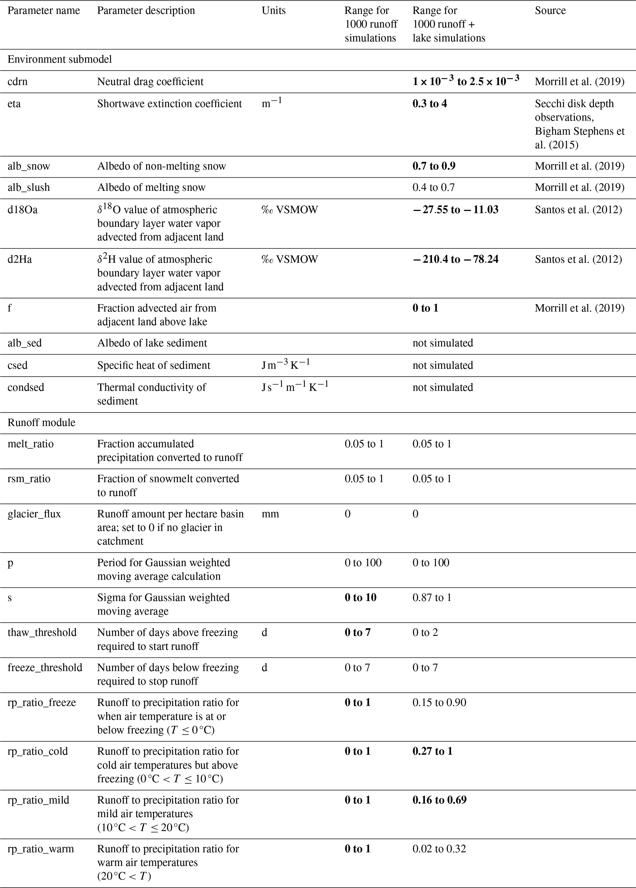
In addition to catchment area, lake area for each depth slice, and maximum depth, ten lake-specific parameters must be prescribed in the model (Table 1). Because values for several of these parameters are difficult to measure in the field, calibration is necessary.

Table 1 Description of lake-specific and runoff parameters with ranges used for Latin Hypercube sampling to generate an ensemble of 1000 simulations. Ranges of sensitive parameters (calibrated range is significantly different from the range of 1000 simulations) in the runoff module calibration were narrowed prior to simulating the temperature and δ²H values of water profiles. Sensitive parameters across calibration to all observations are shown in bold text. Parameters are unitless unless otherwise noted.

2.2 Runoff module

We adapt a simple runoff module from Cluett (2021) to be flexible to any catchment. The module calculates the amount and isotope values of runoff based on daily air temperature, precipitation amount, and isotope values in precipitation. These runoff module outputs force the environment submodel, which converts and transforms input runoff amounts into volume in meters cubed by multiplying amounts by the prescribed catchment area. The module also estimates the amount and isotope values of snow accumulated in the catchment and its isotope values, which are not required to force the environment submodel but could be useful to compare with observations, if available.

The runoff module has 11 tunable parameters that control the runoff amount and isotope value at any given time step (Table 1). Runoff-to-precipitation ratios describe the proportion of precipitation that becomes runoff rather than evaporating or being stored in soils. The model uses four distinct runoff-to-precipitation ratio parameters, each triggered by a specific air temperature range (which can be tailored to the site by the user) to represent different hydrological regimes. To simulate gradual freeze-up in the fall and thaw in the spring, the “thaw_threshold” and “freeze_threshold” parameters dictate the number of days needed to start or stop runoff, respectively. If snow has accumulated in the catchment, the “melt_ratio” controls the fraction of accumulated snow that is converted to meltwater each time step. The “rsm_ratio” partitions the meltwater between immediately contributing to runoff and short-term storage in snowpack. A fraction of meltwater from the previous accumulation contributes to runoff in the current time step, while the remaining fraction (1−“rsm_ratio”) is trapped and released with a one-time step delay. If a glacier is present in the catchment, the “glacier_flux” parameter can be set, which supplies an amount of meltwater in millimeters from that source relative to the catchment area. Isotope values in runoff from glacial meltwater default to the minimum isotope values in precipitation supplied in the meteorological input file or can be specified by the user.

Runoff amount in millimeters at each time step is calculated from the contributing water sources (current precipitation amount that becomes runoff, meltwater from recent accumulation, the prescribed glacier flux, and meltwater from older stored accumulation in the catchment) as follows, where i is the ith time step.

$$\begin{array}{}\text{(1)}& \begin{array}{rl}{\text{Runoff}}_i& =({\text{Precip}}_i\cdot \text{rp\_ratio})\\ & +({\text{Acc}}_{i-\mathrm{1}}\cdot \text{melt\_ratio}\cdot \text{rsm\_ratio})\\ & +({\text{Acc}}_{i-\mathrm{2}}\cdot \text{melt\_ratio}\cdot (\mathrm{1}-\text{rsm\_ratio}\left)\right)\\ & +\text{glacier\_flux}\end{array}\end{array}$$

At each time step where the air temperature and amount of precipitation result in runoff into the lake, the δ²H and δ¹⁸O values in runoff are calculated as a mixture of each of the contributing water sources described above, where the δ²H and δ¹⁸O values in each source are weighted by its contribution to total runoff amount at that time step.

$$\begin{array}{}\text{(2)}& {\displaystyle }\begin{array}{rl}\mathit{\delta }{}^{\mathrm{2}}\mathrm{H}& {\text{Runoff}}_i=\left({\displaystyle \frac{{\text{Precip}}_i\cdot \text{rp\_ratio}\cdot \mathit{\delta }{}^{\mathrm{2}}\mathrm{H}{\text{Precip}}_i}{{\text{Runoff}}_i}}\right)\\ & +\left({\displaystyle \frac{{\text{Acc}}_{i-\mathrm{1}}\cdot \text{melt\_ratio}\cdot \text{rsm\_ratio}\cdot \mathit{\delta }{}^{\mathrm{2}}\mathrm{H}{\text{Acc}}_i}{{\text{Runoff}}_i}}\right)\\ & +\left({\displaystyle \frac{{\text{Acc}}_{i-\mathrm{2}}\cdot \text{melt\_ratio}\cdot \left(\mathrm{1}-\text{rsm\_ratio}\right)\cdot \mathit{\delta }{}^{\mathrm{2}}\mathrm{H}{\text{Acc}}_{i-\mathrm{2}}}{{\text{Runoff}}_i}}\right)\\ & +\left({\displaystyle \frac{\text{glacier\_flux}\cdot \mathit{\delta }{}^{\mathrm{2}}\mathrm{H}{\text{Glacier}}_i}{{\text{Runoff}}_i}}\right)\end{array}\text{(3)}& {\displaystyle }\begin{array}{rl}\mathit{\delta }{}^{\mathrm{18}}\mathrm{O}& {\text{Runoff}}_i=\left({\displaystyle \frac{{\text{Precip}}_i\cdot \text{rp\_ratio}\cdot \mathit{\delta }{}^{\mathrm{18}}\mathrm{O}{\text{Precip}}_i}{{\text{Runoff}}_i}}\right)\\ & +\left({\displaystyle \frac{{\text{Acc}}_{i-\mathrm{1}}\cdot \text{melt\_ratio}\cdot \text{rsm\_ratio}\cdot \mathit{\delta }{}^{\mathrm{18}}\mathrm{O}{\text{Acc}}_i}{{\text{Runoff}}_i}}\right)\\ & +\left({\displaystyle \frac{{\text{Acc}}_{i-\mathrm{2}}\cdot \text{melt\_ratio}\cdot \left(\mathrm{1}-\text{rsm\_ratio}\right)\cdot \mathit{\delta }{}^{\mathrm{18}}\mathrm{O}{\text{Acc}}_{i-\mathrm{2}}}{{\text{Runoff}}_i}}\right)\\ & +\left({\displaystyle \frac{\text{glacier\_flux}\cdot \mathit{\delta }{}^{\mathrm{18}}\mathrm{O}{\text{Glacier}}_i}{{\text{Runoff}}_i}}\right)\end{array}\end{array}$$

3 Methods

3.1 Study sites

We simulate two lakes located in western New York State with contrasting morphometry, hydrology, and mixing regimes (Fig. 1). Red Pond (42.1333° N, −78.9128° W) is a small meromictic kettle pond with no channelized inflow or outflow, and a maximum depth of 18 m. The lake surface area is approximately 1 ha, and the 10 ha catchment is forested and steeply sloping. Bear Lake (42.3470° N, −79.3840° W) is a large, dimictic lake with two inflows and one outflow that are channelized and constantly flowing. The maximum depth of 8 m is shallow compared to Red Pond. Bear Lake's surface area is 49 ha with a 2600 ha catchment. Both lakes experience ice cover during winter, with ice-off occurring late March to early April and ice-on mid-December to mid-January. Because the lakes are within 2 h by car from the University at Buffalo's campus, frequent monitoring was possible.

Figure 1 Maps of study area. (a) Map of western New York State showing locations of study lakes, observed isotope values in precipitation, streamflow observations, and weather stations relevant to model inputs. Inset map shows location in eastern North America. Bathymetric maps of (b) Bear Lake and (c) Red Pond showing locations of monitoring and moorings (stars). 2 m LiDAR from https://data.gis.ny.gov/ (last access: 25 July 2025). Colormap from Crameri et al. (2020).

3.2 Observational datasets

We collected multi-year observations of temperature and isotope values in Red Pond and Bear Lake to calibrate the environment submodel (Table 2; Topness and Thomas, 2026a, b).

Table 2 Observational data used for bias correction, model inputs, calibration, and validation.

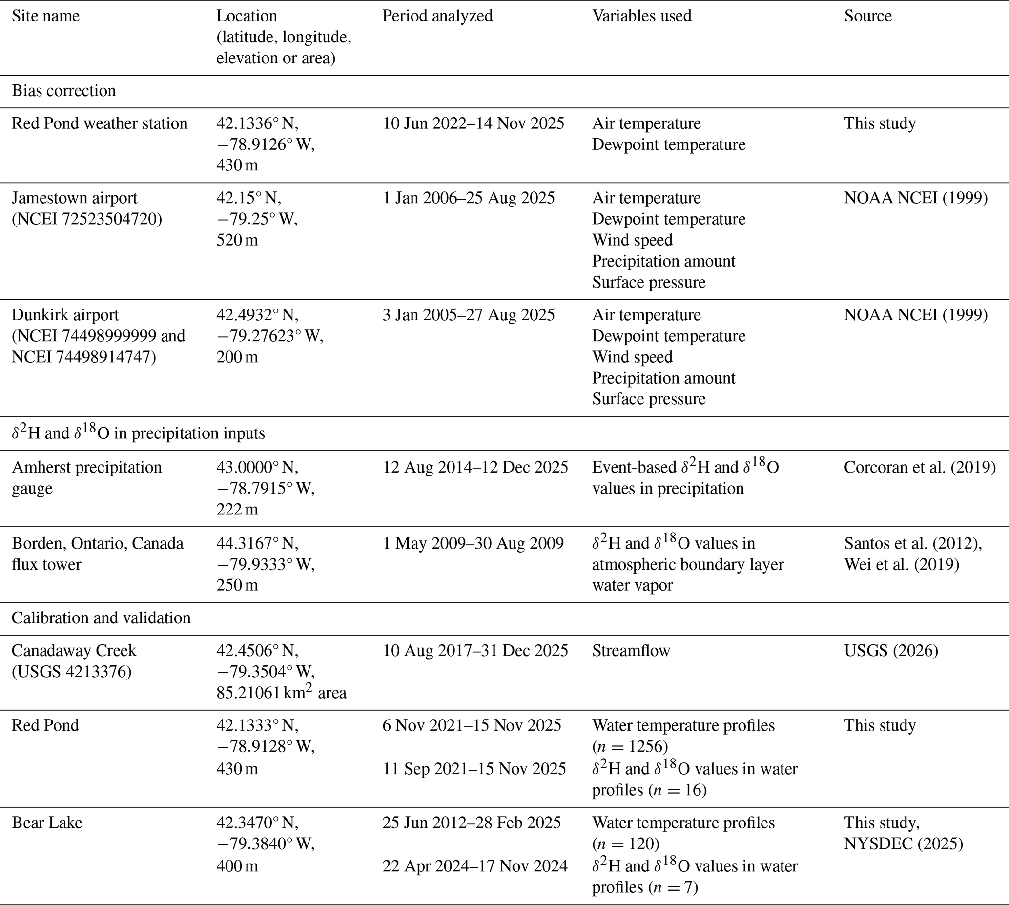
Most water temperature observations were measured continuously by thermistor strings. We deployed HOBO UTBI-001 temperature loggers (Red Pond: approximately 1, 2, 8, and 18 m; Bear Lake: approximately 1 and 7 m; temperature accuracy: ±0.21 °C) and a HOBO U20L-01 temperature and water level logger (Red Pond: 4.6 m; Bear Lake: 4 m; temperature accuracy: ±0.44 °C) to monitor at 30 min intervals. To correct for slight changes in logger depths between deployment periods, we calculated water pressure from the water level logger and estimated the distance of each instrument (which is fixed) relative to the location of the water level logger on the string. We computed daily average temperatures only for days where there are observations over the full day (i.e. no half-days) at each depth, which best matches environment submodel output (daily average of each 1 m depth layer). We also collected temperature profiles with measurements at every meter from surface to bottom using a Yellow Spring Instruments EXO3 multiparameter water quality sonde (temperature accuracy: ±0.01 °C; Fig. S1 in the Supplement). For Bear Lake, we supplemented our observations with temperature profiles from the New York State Department of Environmental Conservation's Division of Water Monitoring Data Portal (NYSDEC, 2025).

To monitor δ²H and δ¹⁸O values in lake water, we collected water samples at depths of 1, 4, 7, 16, and 18 m at Red Pond, due to its depth and stability, and every meter at Bear Lake using a Nansen bottle (Aquatic Research Instruments; Fig. S1). We stored samples at 4 °C in capped and Parafilm-sealed 4 mL glass vials with no head space. We filtered water samples using 0.2 µm hydrophilic Teflon filters into 2 mL glass vials before analysis. We measured δ²H and δ¹⁸O values in water samples using a Picarro L2130-i Wavelength-Scanned Cavity-Ring Down Spectrometer with a V1102-i vaporization module and CTC Analytics Prep and Load autosampler at the University at Buffalo Organic and Stable Isotope Biogeochemistry Laboratory (UB OSIBL). We measured each sample four times, discarding the first injection, and reported the average value of the last three injections. We calibrated measured values using UB OSIBL standards that span a range of −265.9 ‰ to +21.4 ‰ for δ²H and −33.61 to +12.41 for δ¹⁸O. The UB OSIBL standards were calibrated using primary standards (GISP, VSMOW2, SLAP2) from the International Atomic Energy Agency (IAEA). We corrected for memory and drift following Van Geldern and Barth (2012). Average standard deviations of replicate measurements were 0.47 ‰ for δ²H and 0.09 ‰ for δ¹⁸O. We reported results using delta notation in per mille (‰) relative to Vienna Standard Mean Ocean Water (VSMOW).

We assess the runoff module's performance using daily average streamflow observations from Canadaway Creek (42.4506° N, −79.3504° W; USGS, 2026). Streamflow observations, which reflect runoff from rainfall and snowmelt, provide a reasonable target for the amount and timing of runoff entering the catchments of our lake study sites. We use these observations for runoff module calibration because Canadaway Creek is the closest monitored stream to our study sites that is not dammed (Fig. 1a). To compare with simulated runoff amounts, we divide the daily average streamflow observations by the drainage area that sources the stream's monitoring gauge (Table 2). We only include observations that have been accepted for publication by USGS.

3.3 Model inputs

We force the environment submodel with daily ERA5 Global Reanalysis Data from 1994 to 2025 (Hersbach et al., 2020, 2023). We extract and average data from the four grid cells that intersect the lake and catchment area (Red Pond: (42° N, −79° W), (42° N, −78.75° W), (42.25° N, −79° W), (42.25° N, −78.75° W) and Bear Lake: (42.25° N, −79.50° W), (42.25° N, −79.25° W), (42.50° N, −79.50° W), (42.50° N, −79.25° W)). We use 6-hourly resolution for all variables except for accumulated variables (precipitation amount, longwave radiation, shortwave radiation), which we download at hourly resolution and then sum to accurately represent daily totals (Fig. S2).

Quantile-mapping is often used to remove bias from reanalysis data (e.g. Morrill et al., 2019), but we do not correct model inputs due to minimal differences with nearby meteorological observations. We compared ERA5 variables with observations from weather stations that are located within the same ERA5 grid cells as their respective lakes (Table 2). At Red Pond, we also monitored daily air temperature and relative humidity using a HOBO U23-001A Pro v2 weather station (temperature accuracy: ±0.2 °C; relative humidity accuracy: ±2.5 %; Topness and Thomas, 2026a). Comparison of Red Pond ERA5 air temperature and relative humidity to our weather station observations from June 2022 to November 2025 reveal the differences were insignificant (Figs. S3 and S4). While wind speed observations from a weather station in Jamestown, New York (NOAA NCEI, 1999) are significantly higher than ERA5 (KS=0.14, p<0.001), we do not correct this variable because Red Pond's location in a kettle hole surrounded by a forested catchment creates low wind speeds at the lake. Observations from a weather station in Dunkirk, New York and ERA5 variables for Bear Lake show some significant differences (NOAA NCEI, 1999; Figs. S5 and S6). Air temperature and wind speed (KS=0.07, p<0.001 and KS=0.15, p<0.001, respectively) are higher than ERA5 in the 90th percentiles. However, we do not quantile-map due to large (∼200 m) elevation differences between Dunkirk and Bear Lake.

Because isotope values in precipitation are not variables available in this reanalysis dataset, we follow previous studies (Corcoran et al., 2021; Holtzman et al., 2025; Jones and Dee, 2018) and use an amount-weighted monthly average climatology to force the environment submodel. We use event-based observations from Amherst, New York spanning August 2014–December 2025 (Corcoran et al., 2019) to build our monthly climatology. While this simplifies the system (i.e. no variability among years), it is necessary because decades-long, continuous observations of isotope values in precipitation are rare (IAEA/WMO, 2015).

We estimate the lake surface and catchment area for both lakes using Google Earth. We surveyed bathymetry using a Humminbird Fishfinder device and plotted results using Autochart software (https://humminbird.johnsonoutdoors.com/us/learn/mapping/autochart, last access: 1 May 2024). Because Red Pond has two basins separated by a sill that is shallower than the maximum summer mixolimnion (4 m depth), we only simulate the larger, western basin from which we collected observations (Fig. 1c). We set the vertical layer thickness parameter to 1 m (dz=1.0), following applications of this model to lakes with similar depths (Martynov et al., 2010; Morrill et al., 2019). For both lakes, we prescribe initial conditions for the temperature, salinity, and δ²H and δ¹⁸O values of water as profile averages of our observations. We perform a model spin-up by simulating ten years of 1994 conditions, then save outputs from 1995 to 2025.

3.4 Establishing parameter ranges

An important step for calibration of model parameters is defining the sampling space (Mai, 2023). We sample from a wide range while ensuring values are physically possible for the study lakes (Table 1). We use suggested ranges from Dee et al. (2018) for all lake-specific parameters, excluding the shortwave extinction coefficient, which is a critical parameter for accurately simulating water temperature (Dee et al., 2018; Morrill et al., 2019). Secchi disk depth observations from Red Pond and Bear Lake, and for 388 lakes in New York State (which we convert using $\mathrm{1.57}/Z_{\text{SD}}=\mathit{\eta }$; Dee et al., 2018) support higher values for the shortwave extinction coefficient (Bigham Stephens et al., 2015) (Fig. S7). Therefore, we update the recommended range from 0.1–1.0 to 0.3–4.0 m⁻¹. We do not simulate thermal impacts from bottom sediments, so do not include the albedo, specific heat, and thermal conductivity of sediment parameters. See Morrill et al. (2019) and https://github.com/carriemorrill/lake-model/ (last access: 1 May 2026) for more details on sediment heat parameters.

We establish parameter ranges for δ¹⁸O values of atmospheric boundary layer water vapor above the lake using minimum and maximum summer (June–August) observations from Borden, Ontario, Canada (44.3167° N, −79.9333° W; Santos et al., 2012) available through the Stable Water Vapor Isotopes Database (Wei et al., 2019). We use this site because of its proximity to our study lakes and similar geographic position downwind from a Laurentian Great Lake (Lake Huron). We calculate δ²H values of atmospheric boundary layer water vapor above the lake based on the Global Meteoric Water Line relationship ($\mathit{\delta }{}^{\mathrm{2}}\mathrm{H}=\mathrm{8}\cdot \mathit{\delta }{}^{\mathrm{18}}\mathrm{O}+\mathrm{10}$). This step removes the need to provide ranges for both δ²H and δ¹⁸O values and ensures these parameters are physically linked. We start with the full range of runoff parameter values as defined by Cluett (2021) and set all runoff-to-precipitation ratios from 0 to 1 (Table 1). We do not use glacier parameters for these simulations because no glaciers exist in the modern lake catchments.

3.5 Runoff module calibration

Given our goal to accurately simulate isotope values in lake water, we aim to reproduce the seasonal distribution of runoff amount for our study sites. Therefore, we calibrate and validate the runoff module using monthly summed runoff amounts estimated using Canadaway Creek streamflow observations (USGS, 2026). Following Morrill et al. (2019), we use even years for calibration and odd years for validation, after confirming the distribution of values in each period are comparable with a Kolmogorov–Smirnov test. We generate 1000 runoff module simulations with parameter sets selected using Latin Hypercube Sampling across the full range of runoff parameter values (Table 2). We evaluate calibration and validation periods using criteria suggested by Moriasi et al. (2007) for monthly streamflow: Nash-Sutcliffe Efficiency (NSE) >0.50, percent bias <25 %, and ratio of the root-mean-square error to the standard deviation of measured data (RSR) ≦0.7. We narrow ranges of sensitive runoff parameters for further use in environment submodel simulations to ensure isotope values in lake water are supported by realistic runoff amounts for the region.

3.6 Environment submodel calibration

Calibration of the environment submodel can require hundreds or thousands of iterations to test possible values of unknown parameters, which are somewhat computationally costly. We establish a parallel processing framework that can be run on a laptop to streamline calibration of lake-specific and runoff parameters. As a general overview of the workflow, the user supplies a comma-separated values (CSV) file with parameter ranges, from which the user can generate the desired number of parameter sets (i.e. 1000) with values selected using Latin Hypercube Sampling (Virtanen et al., 2020). The runoff module automatically runs, using parameter sets to calculate runoff variables and append them to meteorological input files. Completed meteorological input files and compiled environment submodels are placed in separate folders with unique labels. Next, compiled models are run and output files saved (as netCDFs or text files) for further analysis. Models run in parallel to speed up run times (default is five models run simultaneously). For example, parallelization allows 1000 models each simulating 30 years on a daily time step to complete in less than 1 h on a laptop, compared to approximately 7 h when run sequentially.

We use this framework to generate 1000 daily profile simulations for the temperature and isotope values of lake water with parameter sets sampled across the full range of lake-specific parameters and the narrowed range for runoff parameters (Table 1). We evaluate each simulation's performance by calculating root-mean-square error (RMSE) between observed and modeled values across all dates and depths, where n is the total number of observations.

$$\begin{array}{}\text{(4)}& \text{RMSE}=\sqrt{{\displaystyle \frac{\mathrm{1}}{n}}{\sum }_{i=\mathrm{1}}^n({\text{Modeled}}_i-{\text{Observed}}_i{)}^{\mathrm{2}}}\end{array}$$

We also calculate bias to investigate the direction of error, where n is the total number of observations. We do not use bias as a metric for calibration.

$$\begin{array}{}\text{(5)}& \text{Bias}={\displaystyle \frac{\mathrm{1}}{n}}{\sum }_{i=\mathrm{1}}^n({\text{Modeled}}_i-{\text{Observed}}_i)\end{array}$$

Modeled values are output as averages of each 1 m depth, so we treat modeled values as layer midpoints and linearly interpolate modeled values to observation depths prior to calculating RMSE. We also check that the approximate timing of ice-off is realistic for the lakes based on local ice cover observations. We select the 30 simulations with the lowest RMSE as our calibrated ensemble.

3.7 Model experiments

We conduct experiments to assess the performance of the PRYSM v2.0 environment submodel using calibration datasets that mimic common observation collection challenges. The experiments require the environment submodel to predict the temperature or δ²H values of the lakes when calibrated using a single observed profile. This is a realistic scenario reflective of short field seasons (e.g. a few days) at remote study sites. We aim to identify which season's observations are most informative and if the minimum number of observations (one profile) is enough to set up the model so it accurately predicts unseen data. To meet that end, we evaluate the success of each calibration through validation against all other profile observations available for that lake. By testing two lakes with contrasting morphometries and mixing regimes, we can investigate if those lake characteristics have any control over the optimal sampling window.

Our experiments use profile observations from Bear Lake and Red Pond and divide the datasets into one calibration profile for each date. Because some dates have a profile made up of observations from every meter, while others only include 3–4 observations between the lake surface and the bottom, we subset the observational datasets so each profile on each date includes the same number of observations spaced approximately evenly from lake surface to bottom. For Bear Lake, each date includes observations at three depths between 0 and 8 m; for Red Pond, each date includes observations at four depths between 0 and 18 m. For Red Pond we target 1.5, 4, 8, and 17 m and for Bear Lake we target 1, 4, and 7 m. Dates are included if observations exist on that date that are equal or less than 1 m away from the target depths. This means that each date has a profile that captures key physics (near-surface, thermocline, bottom) and equalizes the number of points used in the calibration on each date so model performance can be compared (Figs. S8 and S9). This results in 1254 profiles of temperature and 15 profiles of δ²H values in Red Pond for the experiments, and 79 profiles of temperature and 6 profiles of δ²H values in Bear Lake for the experiments.

We use the 1000 daily profile simulations of temperature and δ²H values in water previously generated and described as a reasonable estimation of parameter uncertainty at a sparsely monitored lake. We calibrate each date by choosing the 30 best-performing (lowest RMSE) simulations from the 1000 total simulations. We evaluate the informativeness of each date's calibration by using observations from all remaining dates and depths as validation. As before, we calculate RMSE as a measure of model performance and to craft guidelines for the most informative sampling season.

4 Results

4.1 Runoff module performance

The PSM does not have a built-in catchment model that would aid in the simulation of both runoff and runoff isotope values (Dee et al., 2018). To address this, we integrate and test a runoff-isotope module with the goal to create plausible runoff amounts and runoff isotope values to force the environment submodel. The calibration period statistics for 21 simulations met the criteria described above for monthly streamflow. Module performance for these simulations remained within the criteria for the validation period. These simulations capture the seasonal timing and amount of runoff for our study sites (Fig. 2), with low runoff in summer months and rain and snowmelt increasing runoff amount in the winter and spring (Hrycik et al., 2024). We identify parameters as sensitive if their calibrated range was significantly (p<0.05) different from the uniform, original parameter range via Kolmogorov–Smirnov test. Sensitive runoff parameters were the “thaw_threshold”, “s” (sigma for the Gaussian weighted moving average), and “rp_ratio_freeze”, “rp_ratio_cold”, “rp_ratio_mild”, and “rp_ratio_warm” (Table 1).

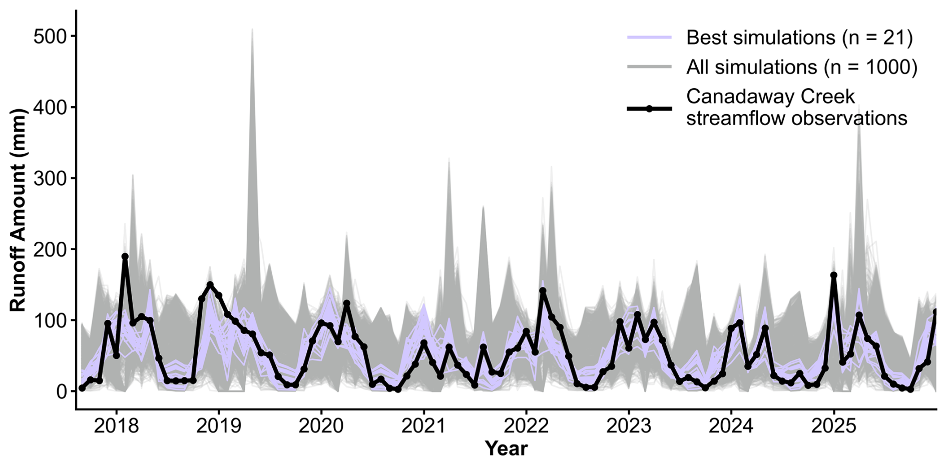
Figure 2 Results of runoff module calibration to drainage area-normalized monthly streamflow from Canadaway Creek (USGS, 2026). We identified the 21 best simulations using criteria from Moriasi et al. (2007).

4.2 Environment submodel performance

The environment submodel accurately reproduces our observed temperature profiles from Bear Lake and Red Pond, two lakes with contrasting mixing regimes. Model strengths include the permanent stratification of Red Pond and the timing of stratified and isothermal periods in Bear Lake (Fig. 3 for subset; see Figs. S10 and S11 for all years). Out of the 1000 total simulations, all parameter sets reproduce the approximate timing of ice-on, so we reject none based on that calibration criteria. We select the 30 best-performing (lowest RMSE) temperature profile simulations for each lake as our calibrated ensemble. The RMSE ensemble average was 1.6 °C for Bear Lake and 0.7 °C for Red Pond (Table 3). The most sensitive parameters for simulating temperature profiles in these lakes are the shortwave extinction and neutral drag coefficients, which parameterize water clarity and evaporation, respectively (Morrill et al., 2019). The calibrated range of the shortwave extinction coefficient is 2.73–3.25 m⁻¹ (Z_SD=0.48–0.58 m) for Red Pond and 0.57–0.73 m⁻¹ (Z_SD=2.15–2.75 m) for Bear Lake, reflecting the high turbidity of these lakes. The Red Pond simulations are additionally sensitive to the albedo of snow, reflecting how Red Pond's smaller surface area may be more responsive to changes in surface energy than Bear Lake. Insensitive parameters were sampled approximately uniformly across their prescribed ranges in the calibrated 30-member ensemble (Fig. S12).

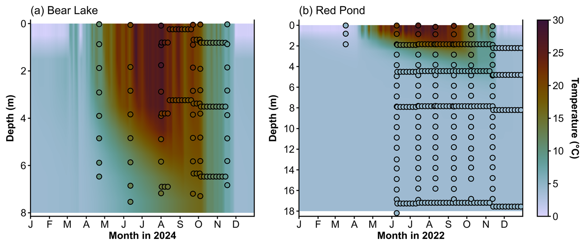
Figure 3 Results of environment submodel calibration to observed water temperature profiles from (a) Bear Lake and (b) Red Pond. Colors are modeled ensemble means for each day and depths. Dots are observations, colored by observed water temperature. Note that we performed calibrations on the full multi-year datasets (shown in Supplement) and only show a subset here. For dense periods of daily observations, we plot every 5th measurement but calibrated to all measurements. Colormap from Crameri et al. (2020).

Table 3 Environment submodel performance for temperature and δ²H values in water profiles, surface, and bottom. RMSE and bias scores are the average results from each calibrated 30-member ensemble. Scores for the profiles are shown in bold text.

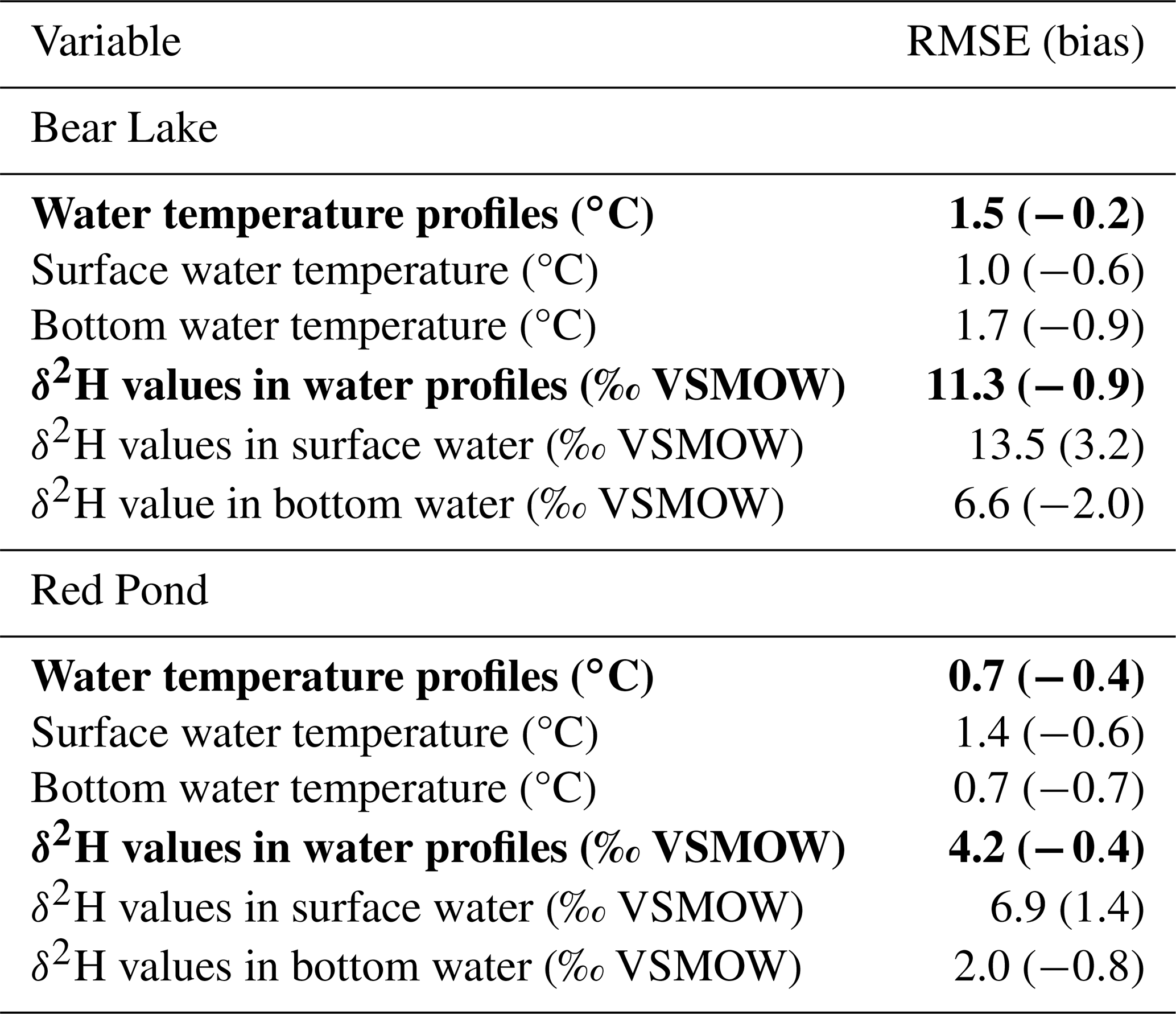
Using our runoff module and framework to prescribe isotope values in precipitation and runoff and drive the environment submodel, seasonal variability in observed δ²H values in Bear Lake and Red Pond is well represented by the simulations (Fig. 4c; see Figs. S13 and S14 for other depths). Our simulations reproduce ²H-enriched summer lake water compared to winter δ²H values in lake water, reflecting the seasonal trends of isotope values in precipitation characteristic of western New York (Fig. 4a; Corcoran et al., 2019). The 30 best-performing simulations of δ²H values in water profiles for each lake result in RMSE ensemble averages of 11.3 ‰ for Bear Lake and 4.2 ‰ for Red Pond, with most misfit coming from the surface/epilimnion (Table 3; Figs. S13 and S14). RMSE ensemble averages for δ²H values in the surface water are 13.5 ‰ and 6.9 ‰ for Bear Lake and Red Pond (Table 3). Given a total observed seasonal range of approximately 40 ‰ for both lakes at the surface, the errors account for 34 % and 17 % of the seasonal range for Bear Lake and Red Pond, respectively. Because water temperature impacts hydrogen isotope fractionation during evaporation, simulated δ²H values in lake water are sensitive to thermal parameters. Other sensitive parameters are the fraction and isotope value of the atmospheric boundary layer water vapor advected from adjacent land and runoff-to-precipitation ratios (Table 1). The best-performing simulations for both lakes use an air mass consisting of more than 50 % advected air (f>0.50). This suggests that the water vapor in the air mass above the lake when our observations were collected was mostly derived from advected air rather than from evaporating lake water. Given the large errors for modeled δ²H values in water profiles compared to temperature profiles, in the next section we explore potential sources of mismatch between the modeled values and observations.

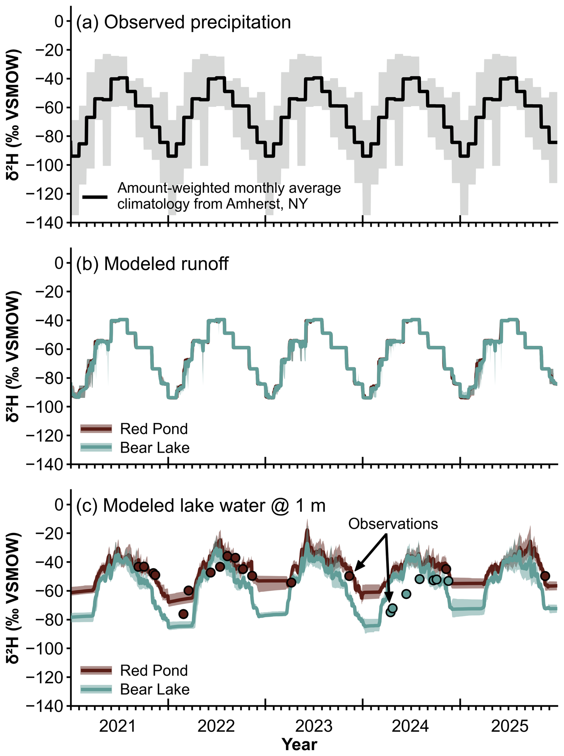
Figure 4 Inputs and outputs for simulating δ²H values in Bear Lake and Red Pond using the environment submodel. Our simulations cover years 1995–2025, but we only show 2021–2025 here where observations overlap with simulations. (a) δ²H values in precipitation based on amount-weighted monthly average observations from Amherst, New York force the runoff module and environment submodel. Gray shading shows the 5th to 95th percentiles of the observations across the entire dataset. (b) Modeled δ²H values in runoff calculated using the runoff module. (c) Results of environment submodel calibration to observations of δ²H values in Red Pond and Bear Lake water. Lines are modeled values at 1 m depth. Dots are observations. In (b) and (c), thick lines are modeled ensemble means and shading shows the 5–95th percentile of the ensemble.

4.3 Investigating the mismatch between modeled and observed δ²H values in lake water profiles

One source of the mismatch between observed and simulated δ²H values in Red Pond and Bear Lake (Fig. 4c) could be parameter uncertainty. To investigate this, we evaluate average ice-free season δ²H values in the epilimnion (average of surface to 3 m depth) for all 30 modeled years across the 1000 simulations for both lakes (Fig. 5). We define the ice-free season as days when the fraction of ice on the lake is zero. We focus on the ice-free season because that is the window most lake sediment proxies reflect (Castañeda and Schouten, 2011). The range of δ²H values for the 1000 simulations is 29 ‰ for Bear Lake and 64 ‰ for Red Pond. For both lakes, runoff parameters have little impact on simulated δ²H values. Thermal and isotope parameters drive the spread in model output for Red Pond, while Bear Lake shows less sensitivity to parameter values. Therefore, errors between observed and simulated δ²H values in Bear Lake may relate to the isotope values of precipitation inputs rather than parameter values.

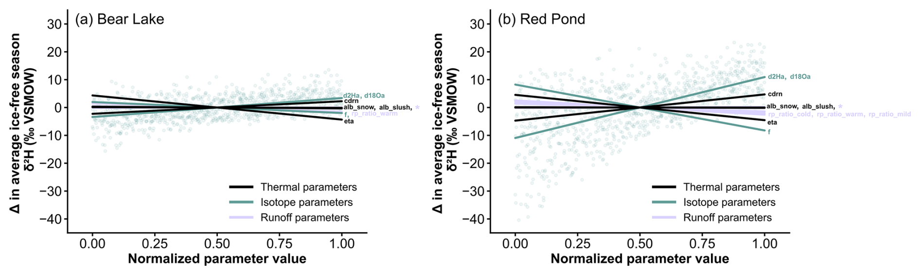
Figure 5 Summary of 1000 simulations of δ²H values in water with different parameters sampled using Latin Hypercube for (a) Bear Lake and (b) Red Pond. Lines are colored by parameter category and represent lines of best fit through the distribution of each parameter across the sampled range for the average ice-free season δ²H values in the epilimnion (surface to 3 m depth) for all 30 years. Parameter values are normalized so they can plot on the same axis (see Table 1 for actual values), and δ²H values are displayed as anomalies from the parameter values at 0.50. Annotations at the end of each line identify individual parameters, where * indicates all runoff parameters not listed. Blue dots show an example of the parameter distribution for one parameter: the δ²H value of the atmospheric boundary layer water vapor.

Another reason for errors between the observations and simulations could be due to uncertainty within the isotope values in precipitation inputs. We force the runoff module and environment submodel with an amount-weighted monthly average climatology from Amherst, New York, which is approximately 85 km northeast of our study sites (Fig. 1a). Therefore, the true isotope values, timing, and amount of rainfall that fell onto the lakes when our observations were collected could be different than the model inputs. Further, using a climatology simplifies the system, but allows for simulations beyond an often short (i.e., a few years) observational window (IAEA/WMO, 2015). To address this, we test different versions of the isotope values in precipitation we use to force the environment submodel to quantify how uncertainty might influence simulated isotope values in lake water. Using the 30-member ensemble from our calibration (Fig. 4c) forced with the amount-weighted monthly average climatology version for isotope values in precipitation inputs, we complete two experiments for each lake using different inputs: the 5th percentile climatology and 95th percentile climatology of the amount-weighted monthly averages from our observations of isotope values in precipitation (as in Fig. 4a). Then, we examine the change in modeled δ²H values in the epilimnion (average of surface to 3 m depth). Simulated ice-free average δ²H values in both Red Pond and Bear Lake are sensitive to the isotope values in precipitation inputs (Fig. 6). Using the 5th percentile climatology, the median ice-free average δ²H values in Bear Lake and Red Pond are 22.2 ‰ and 17.9 ‰ ²H-depleted relative to simulations forced using the average climatology. Using the 95th percentile climatology, the median ice-free average δ²H values in Bear Lake and Red Pond are 17.9 ‰ and 14.8 ‰ ²H-enriched relative to simulations forced using the average climatology.

Figure 6 We tested the sensitivity of modeled δ²H values in Red Pond and Bear Lake when the environment submodel is forced with different climatologies of isotope values in precipitation. Open black circles show the ice-free season (April–November) average of either the monthly amount-weighted 5th or 95th percentile climatology (see Fig. 4a). Box plots show average ice-free season δ²H values of the epilimnion (surface to 3 m depth) across all 30 years for each of the 30 ensemble members using different inputs. For each box plot, horizontal lines show the median average ice-free δ²H value in Red Pond and Bear Lake across the ensemble, the box indicates the 25th to 75th quartile range, and the whiskers display the minimum and maximum values.

4.4 Effects of limited calibration data on environment submodel performance

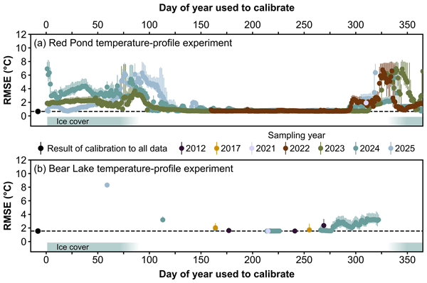
When only a single observed temperature profile is available, the performance of the Red Pond and Bear Lake environment submodels remains reliable and robust. The best-performing environment submodel ensembles result from calibration on temperature profiles collected during the warm, ice-free period dates (Fig. 7). However, performance varied widely by season. The 30-member ensemble average RMSE on any given date in our dataset ranged from 0.7 to 7.0 °C for Red Pond and 1.5 to 8.3 °C for Bear Lake. Dates with the highest ensemble average RMSE values, and the most ensemble spread, occur with environment submodel calibration to temperature profiles that were collected when the lakes were ice-covered. However, the under-ice RMSE scores are not consistent among years (at Red Pond), perhaps due to differences in ice cover conditions (e.g. ice thickness, ice break-up and refreeze, etc). We only have one under-ice temperature profile from Bear Lake, but it also has the highest RMSE of any date tested from that dataset. We identify the warm, ice-free period (in these lakes, ∼ day of year 125–265, or early May to late September) as the most informative sampling window for simulation of both Red Pond and Bear Lake temperature profiles. On these dates, ensemble average RMSE values are almost equivalent as calibration to all water temperature observations (Table 3), and RMSE values are consistent across sampling years. The RMSE for water temperature profiles during this window span 0.7 to 2.0 °C for Red Pond and 1.5 to 2.0 °C for Bear Lake. These RMSE scores are comparable to performance metrics from other studies applying this model (Almeida et al., 2022; Martynov et al., 2010; Perroud et al., 2009; Sae-Lim et al., 2025) and other lake water temperature models (Jia et al., 2021; Ladwig et al., 2024; Martynov et al., 2010; Read et al., 2019).

Figure 7 Effect of environment submodel calibration to an observed water temperature profile from one date as measured by root-mean-square error (RMSE) for (a) Red Pond and (b) Bear Lake. We calibrated each date by choosing the 30 best-performing simulations from 1000 total simulations. RMSE values reflect model performance over the validation period (all remaining observations). Dots show the ensemble average RMSE and bars show the 5th and 95th percentile RMSE of the ensemble, colored by the year the profile was sampled. We show the result of environment submodel calibration to all water temperature observations (as in Fig. 3) for each lake as a black dot. Colormap from Crameri et al. (2020).

Environment submodel calibration to observations of δ²H values in water profiles from one date have a less clear trend regarding which dates are most informative. Generally, summer dates have the lowest RMSE and show the most agreement among ensemble members (Fig. 8). The 30-member ensemble average RMSE for any given date in our dataset ranged from 4.3 ‰ to 8.8 ‰ for Red Pond and 12.8 ‰ to 15.5 ‰ for Bear Lake. From the Red Pond experiment, most dates result in an RMSE score similar to calibration using all observations of δ²H values (Table 3), with dates under-ice or within a few weeks after ice-off being the worst-performing. For Bear Lake, calibration to spring and summer dates resulted in the lowest RMSE scores.

Figure 8 Effect of environment submodel calibration to an observed profile of δ²H values in water from one date as measured by root-mean-square error (RMSE) for (a) Red Pond and (b) Bear Lake. We calibrated each date by choosing the 30 best-performing simulations from 1000 total simulations. RMSE values reflect model performance over the validation period (all remaining observations). Squares show the ensemble average RMSE and bars show the 5th and 95th percentile RMSE of the ensemble, colored by the year the profile was sampled. We show the result of environment submodel calibration to all observations of δ²H values (as in Fig. 4c) for each lake as a black square. Colormap from Crameri et al. (2020).

5 Discussion

PSMs support mechanistic interpretations of paleoclimate data from lake sediments that incorporate uncertainty. However, two obstacles hinder their wider use: (1) lack of long-term, continuous observations of isotope values in precipitation and a built-in catchment model make simulating isotope values in lake water challenging, and (2) observational datasets for environment submodel calibration are often sparse. Most lakes are not well-monitored (Stanley et al., 2019), especially remote sites where few observations can be collected and sites from which paleoclimate datasets have been generated but cannot be easily revisited. We integrate a runoff-isotope module into the PSM and craft guidelines for the most useful observations for environment submodel calibration to help overcome these obstacles.

5.1 Modeled temperature outperforms δ²H values of lake water profiles

Bear Lake and Red Pond thermal dynamics are well-represented in our simulations, as indicated by low RMSE scores when calibrated to all available water temperature profile observations (Table 3). Yet, the ensemble average RMSE for Bear Lake is more than two times higher than for Red Pond. This likely stems from Red Pond's greater stability as a meromictic lake, in which water column temperatures are largely unchanging year to year below 8 m depth. Meanwhile, Bear Lake mixes completely twice a year, meaning that the temperature of the entire water column responds to atmospheric conditions (Fig. 3). The shortwave extinction coefficient is a sensitive parameter for simulating temperature profiles in these lakes (Table 1; Fig. S12). All parameters in the environment submodel are static and do not change throughout the simulations. However, Secchi disk depth observations from Bear Lake illustrate seasonally changing water clarity, and therefore shortwave extinction coefficient (Fig. S7). Allowing seasonal or yearly flexibility in this parameter could be useful for improving model fit further, given that water clarity can vary over time and this could be reflected in multi-year observational datasets used for calibration.

Modeled δ²H values in Bear Lake and Red Pond water reproduce the approximate magnitude and seasonal timing of our observations (Fig. 4), but errors are large compared to simulated temperature profiles. We explored parameter uncertainty and isotope values in precipitation inputs as two potential sources of error. For Red Pond, thermal and isotope parameters lead to a large spread in modeled δ²H values in the epilimnion during the ice-free season (Fig. 5). This makes sense because those parameters impact evaporation amount and hydrogen isotope fractionation during evaporation, which strongly influence the δ²H values in Red Pond as a closed-basin lake. Because Bear Lake is hydrologically open and receives substantial runoff due to its large catchment, its hydrogen isotope composition is less strongly influenced by thermal and isotope parameters. For open-basin systems like Bear Lake, the modeled δ²H values in the epilimnion are more sensitive to the δ²H values in precipitation inputs. Despite uncertainties with simulating δ²H values in these lakes using the environment submodel, we view them as useful representations of the two lake systems on seasonal and longer timescales. Proxy time series in lake sediments often integrate years to decades within a single sample. Therefore, daily model outputs can be aggregated to interannual or interdecadal time scales to obtain values that are directly comparable to proxies (e.g. Morrill et al., 2019).

Monitoring of isotope values in precipitation is essential to better modeling of δ²H values in lake water (Birkel et al., 2025; Jones et al., 2016). Quality meteorological inputs are critical given that the accuracy of the environment submodel and application of the PSM to interpret proxy time series from lake sediments depends on the accuracy of the calibration to the modern lake system. The climatology of isotope values in precipitation that we use as input has larger uncertainties than other variables that force the lake model (e.g. air temperature or shortwave radiation). Models that simulate isotopes values in lake water seem to perform best when forced with local, daily observations rather than a climatology (Hostetler and Benson, 1994; Jones et al., 2016; Steinman et al., 2010). However, using daily observations limits the simulation to the window when observations were collected, making it difficult to use the environment submodel to simulate isotope values in lake water over time periods long enough to answer paleoclimate questions. Another potential solution to improve model performance given currently limited monitoring is parameterization of the isotope values in precipitation inputs to help constrain and characterize uncertainty within the data and allow for year-to-year variability.

5.2 Observations from the warm, ice-free season are most informative for environment submodel calibration

We show that sparse observations of temperature and δ²H values in lake water can result in reliable and robust environment submodel calibration for proxy system modeling applications. We find that environment submodel calibration to a single profile observation measured during the warm, ice-free season (for these lakes, early May to late September), when the lakes are most stable, results in the selection of parameter sets that generalize the best to unseen data from other years and water depths. We show that performance measured by RMSE in the validation period for simulated water temperature profiles of two mid-latitude lakes calibrated to a single summer observed profile is less than or equal to 2 °C, which is small relative to large uncertainties in proxy calibrations. The RMSE of the validation period for simulated δ²H values in water profiles results in larger errors compared to temperature, even when calibrated to many (n>6) profile observations. We attribute these errors to uncertainties within the isotope values in precipitation inputs (Fig. 6) rather than lake-specific or runoff parameter uncertainty. However, observations measured on summer dates seem to be the most informative.

Several factors explain why water temperature profiles from the warm, ice-free season are the most informative for environment submodel calibration. In this model, the thermal parameters with the most influence on water temperatures (shortwave extinction and neutral drag coefficients) are most sensitive to the ice-free season. The shortwave extinction coefficient controls how deeply solar radiation can penetrate the water column, and thus the strength of stratification. Because parameters are constant for the entire simulation, summer water temperature profiles capture the period of maximum summer stratification, thus are most informative for constraining that uncertain parameter. The neutral drag coefficient describes surface roughness, which impacts wind-driven mixing and evaporation, and therefore becomes unimportant when the lake is ice-covered. In Fig. 7, calibration for under-ice dates has a large spread in RMSE scores among the 30 ensemble members, illustrating the disagreement among parameter sets due to observations not sufficiently constraining parameter values. The few weeks before ice-on and after ice-off are also unsatisfactory calibration targets. When the lake is isothermal (or in the case of Red Pond, the metalimnion is isothermal), the thermal stability is weaker, and thus observations from those dates are also less informative.

Environment submodel calibration to δ²H values in Bear Lake and Red Pond is more complex and controlled by thermal parameters as well as runoff and isotope-specific parameters, which means that observational datasets must reflect several processes. Unlike the temperature profile experiment, the δ²H values in water profiles experiment for Red Pond and Bear Lake shows different trends in the most informative dates for environment submodel calibration. This likely stems from the stability of Red Pond compared to Bear Lake, and the lakes' contrasting hydrologic characteristics. As shown in Fig. 6, δ²H values in Bear Lake closely track δ²H values in precipitation, which is a similar result as the simulation of open-basin lakes in other lake models (Jones et al., 2016). Meanwhile, closed-basin lakes like Red Pond are dominated by an evaporation signal, where short-term variability in δ²H values in precipitation inputs has a smaller impact on simulated δ²H values in lake water (Hostetler and Benson, 1994; Jones et al., 2016; Steinman et al., 2010). Because Red Pond's morphology and hydrology make the lake less sensitive to δ²H in precipitation, a single δ²H profile from the ice-free season can constrain environment submodel parameters that generalize well to other years and water depths. While this is the case for Red Pond, other closed-basin lakes may be more sensitive to δ²H values in precipitation depending on their outseepage and morphometry (Steinman et al., 2010). Outseepage can provide a pathway for a closed-basin lake to lose water other than evaporation. For example, if the rate of water outflow through seepage is high and the lake's surface area is small relative to its volume, evaporation might not buffer δ²H values in lake water in the same way. In any case, the δ²H values in precipitation inputs should be chosen carefully, but especially when using the environment submodel to simulate open-basin lakes with large catchments that are sensitive to inputs.

5.3 Limitations

We aimed to provide environment submodel calibration and sampling guidelines that apply to many different lakes and support our guidelines with results from two lakes with contrasting morphometries, mixing regimes, and hydrology. Our study lakes represent two endmember systems with respect to temperature and δ²H values of water profiles. However, we acknowledge that both of our study sites are in the same region and experience the same climate. Climate controls the length of the ice-free season, and thus the strength of stratification and amount of evaporation, runoff, and precipitation entering the lake. Therefore, the most informative sampling window will likely change depending on lake location. For example, Arctic lakes have a shorter ice-free season than lakes in the mid-latitudes (Arp et al., 2010). This would shorten the window for when the most informative observations could be collected. Additionally, the sampling guidelines we describe most likely only apply to temperate lakes. Lakes that mix more frequently, such as shallow polymictic lakes found in the tropics and subtropics (e.g. Mosquera et al., 2025) or lakes that are permanently ice-covered, may have different windows where observations are most informative. Despite this, the tools, runoff module, and calibration framework we describe are adaptable for simulating any lake system and therefore can be used to assess performance in other climates.

Another limitation when applying the PSM to interpret paleoclimate data is whether environment submodel parameter values remain constant over time. While modern observations are critical for selecting the best-performing parameter sets that reproduce the lake system, some processes that these parameters represent may change across paleoclimate time scales. For example, a lake catchment that hosted glaciers in the past but lacks them today may have experienced shifts in water clarity over time. This may render a shortwave extinction coefficient calibrated using modern observations inadequate for paleoclimate simulations. Similarly, past climate regimes could alter runoff-to-precipitation ratios, shifting both the amount and isotope values of runoff. Our runoff module offers some flexibility in this regard because several parameters control runoff-to-precipitation ratios and they are each only activated when user-specified air temperature thresholds are met. Testing the sensitivity of environment submodel parameters using the framework developed here could evaluate the impact key parameters have on a lake system prior to using the PSM to compare modeled values with paleoclimate data.

6 Conclusion

In this paper, we addressed two obstacles hindering the broad use of PSMs for interpretation of lake sediment archives. We developed and tested a runoff-isotope module, which aids the PSM's environment submodel in simulating hydrogen and oxygen isotope values in lake water. Using a parallel processing framework to rapidly run the environment submodel and thoroughly sample the parameter space, we reproduced observations of temperature and δ²H values in water profiles at two mid-latitude lakes with contrasting characteristics. Given limitations for isotope values in precipitation inputs, our modeling framework may not be well-suited for simulating the response of δ²H values in lake water to high frequency precipitation events, but useful for investigating paleoclimate questions over seasonal or longer timescales. Because paleoclimate data from lake sediments often integrate years or decades within a single sample, daily proxy system model outputs can be aggregated for direct comparison with proxy time series. Through model experiments, we showed that sparse observational data does not necessarily hinder environment submodel performance. When time, resources, or site location limit field season duration, we recommend targeting observations from the warm, ice-free season, which were most informative for calibration of Bear Lake and Red Pond. These contributions will advance proxy system modeling by reducing time spent on model set-up and calibration. These tools and framework are a step towards unlocking the vast global database of paleoclimate time series from lake sediments as climate model validation targets able to improve our ability to predict and prepare for a warmer world.